EECS 556 – Image Processing– W 09

Interpolation

• Interpolation techniques• B‐splines

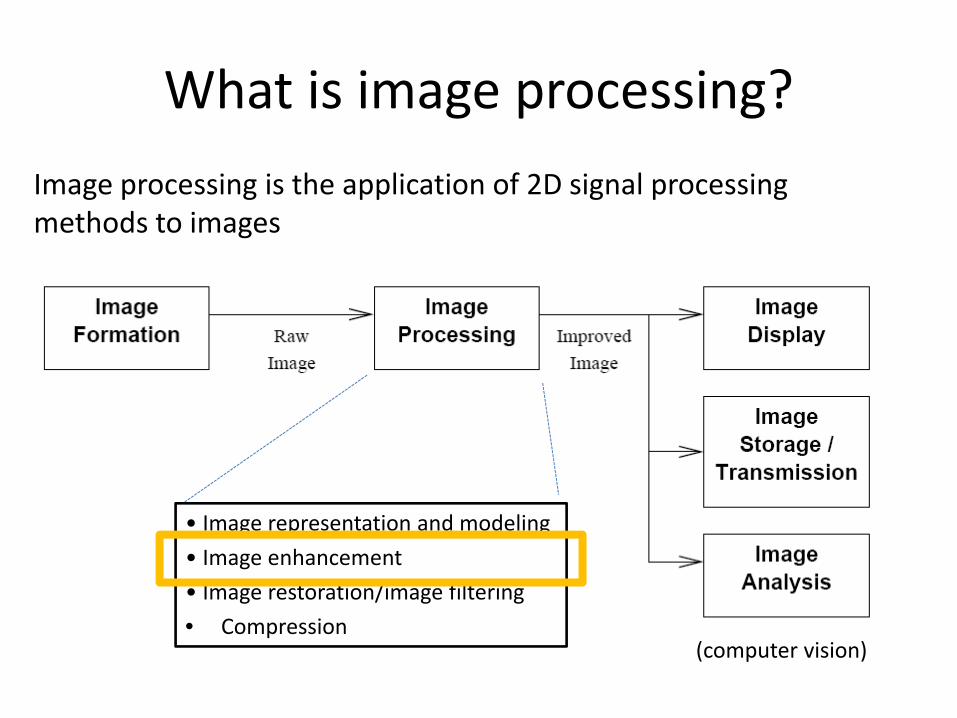
What is image processing?

Image processing is the application of 2D signal processing methods to images

• Image representation and modeling

• Image enhancement

• Image restoration/image filtering

• Compression(computer vision)

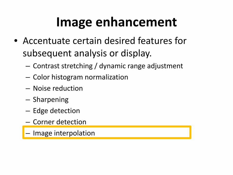
Image enhancement• Accentuate certain desired features for subsequent analysis or display.– Contrast stretching / dynamic range adjustment

– Color histogram normalization

– Noise reduction

– Sharpening

– Edge detection

– Corner detection

– Image interpolation

What is interpolation?• given a discrete‐space image gd[n,m]

• This corresponds to samples of some continuous space image ga(x, y)

• Compute values of the CS image ga(x, y) at (x,y) locations other than the sample locations.

gd[n,m]ga(x, y) g’d[n,m]

What is interpolation?

• Interpolation is critical for:

– Displaying

– Image zooming

– Warping

– Coding

– Motion estimation

Is perfect recovery always possible?

No, (never actually), unless some assumptions on ga(x,y) are made

There are uncountable infinite collection of functions ga(x, y) that agree with gd[n,m] at the sample points

What are these assumptions?• ga must be band‐limited

• Sampling rate must satisfy Nyquist theorem

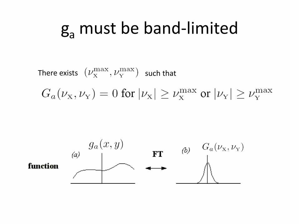
ga must be band‐limited

There exists such that

Sampling rate must satisfy Nyquisttheorem

v v v

Ideal Uniform Rectilinear Sampling

• 2D uniformly sampled grid

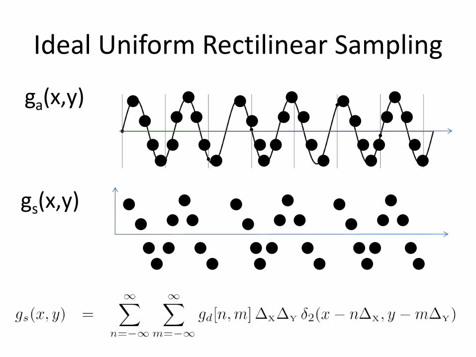
Ideal Uniform Rectilinear Sampling

ga(x,y)

gs(x,y)

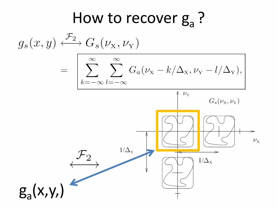
How to recover ga ?

ga(x,y,)

How to recover ga ?

Sinc interpolationWe can recover ga(x, y) by interpolating the samples gd[n,m] using sinc functions

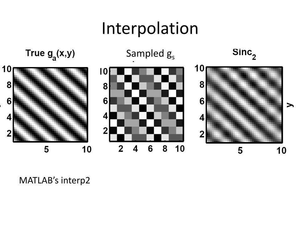
InterpolationSampled gs

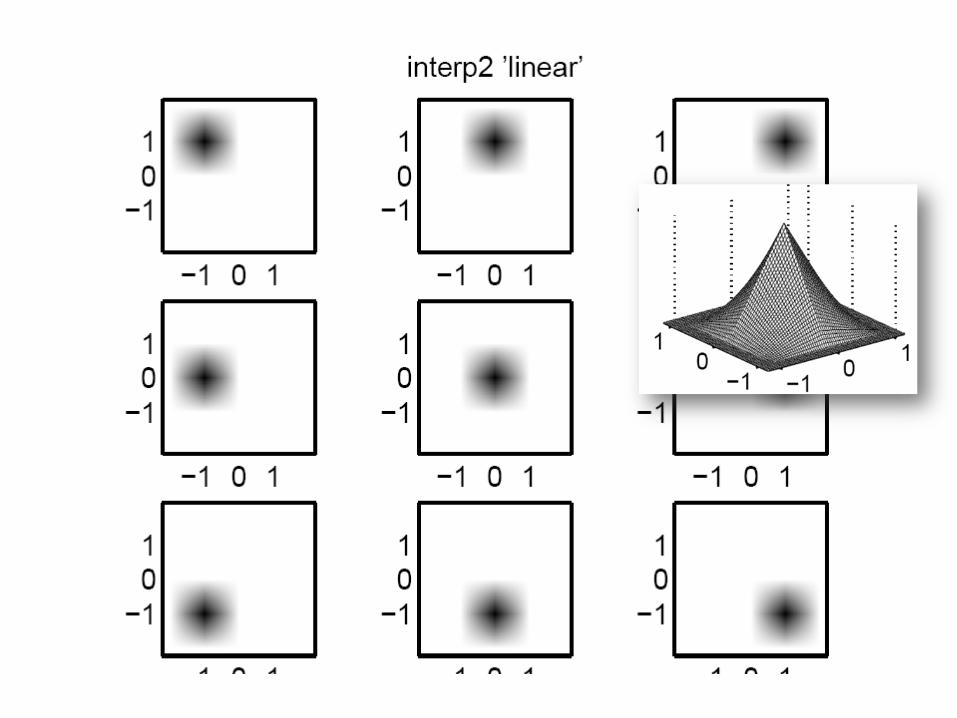
MATLAB’s interp2

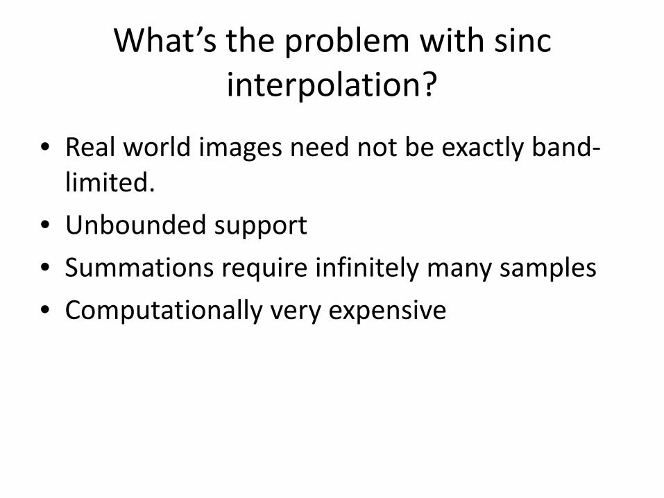
What’s the problem with sincinterpolation?

• Real world images need not be exactly band‐limited.

• Unbounded support

• Summations require infinitely many samples

• Computationally very expensive

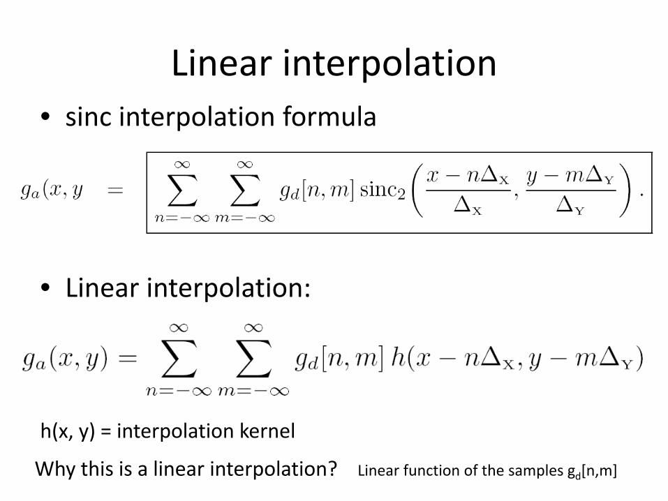
Linear interpolation• sinc interpolation formula 

• Linear interpolation:

h(x, y) = interpolation kernel

Why this is a linear interpolation? Linear function of the samples gd[n,m] 

Linear interpolation

• Consider alternative linear interpolation schemes that address issues with:– Unbounded support

– Summations require infinitely many samples

– Computationally very expensive

Basic polynomial interpolation

Here kernels that are piecewise polynomials

• Zero‐order or nearest neighbor interpolation– Use the value at the nearest sample location

– Kernels are zero order polynomials 

Nearest neighbor interpolation

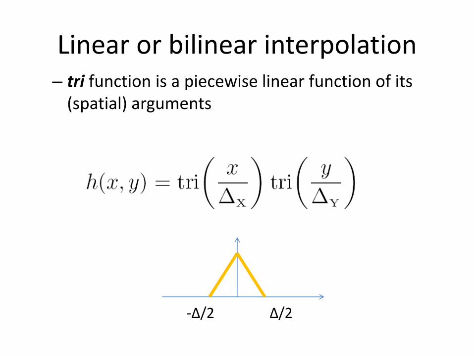
Linear or bilinear interpolation– tri function is a piecewise linear function of its (spatial) arguments 

Δ/2‐Δ/2

Linear or bilinear interpolation• For any point (x, y), we find the four nearest sample point

• fit a polynomial of the form

• Estimate alphas from system of 4 equations in 4 unknowns: 

Interpolating formula (x∈ [0, 1] × [0, 1]):

Linear or bilinear interpolation

1

1

If x∈ [‐1, 1] × [‐1, 1]: 

‐1

0

Linear or bilinear interpolation

Linear interpolation by Delaunay triangulation

Use a linear function within each triangle (three points determine a plane).

MATLAB’s griddata with the ’linear’ opt

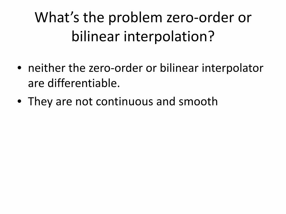
What’s the problem zero‐order or bilinear interpolation?

• neither the zero‐order or bilinear interpolator are differentiable.

• They are not continuous and smooth 

Desirable properties of interpolators

• “self consistency”:

• Continuous and smooth (differentiable):

• Short spatial extent to minimize computation

Desirable properties of interpolators

• Frequency response approximately rect().

• symmetric

• Shift invariant

• Minimum sidelobes to avoid ringing “artifacts”

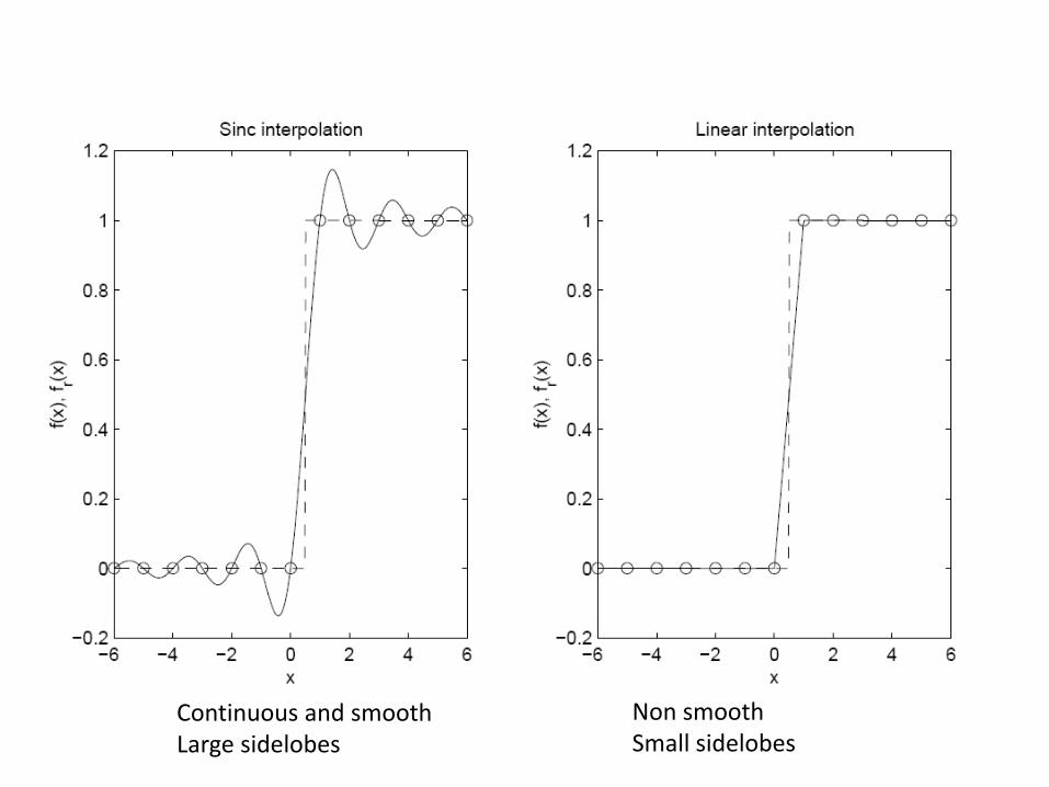
Continuous and smoothLarge sidelobes

Non smoothSmall sidelobes

Non smooth; non shift invariant

Polynomial interpolation– Cubic

– Quadratic

– B‐splines

interpolation kernel:

B‐spline interpolation

• Motivation:– n‐order differentiable

– Short spatial extent to minimize computation

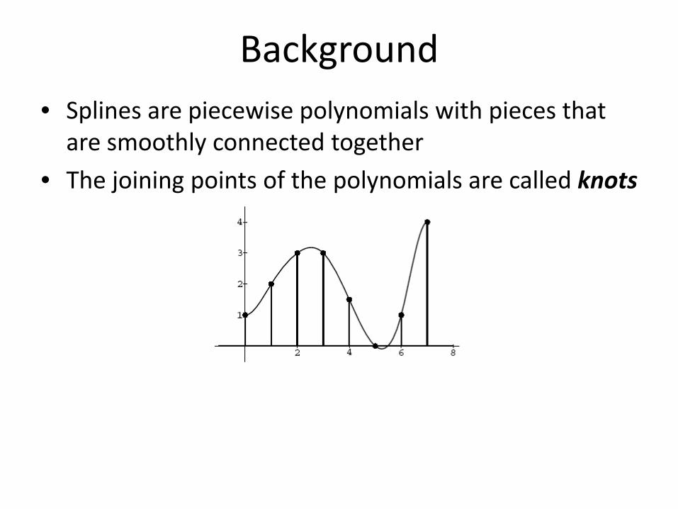
Background • Splines are piecewise polynomials with pieces that are smoothly connected together

• The joining points of the polynomials are called knots

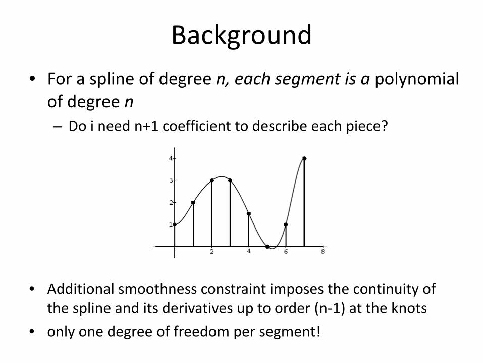
Background • For a spline of degree n, each segment is a polynomial of degree n– Do i need n+1 coefficient to describe each piece?

• Additional smoothness constraint imposes the continuity of  the spline and its derivatives up to order (n‐1) at the knots

• only one degree of freedom per segment!

B‐spline expansion 

• Splines are uniquely characterized in terms of a B‐spline expansion

= central B‐spline = basis (B) spline

integer shifts of the central B‐spline of degree n

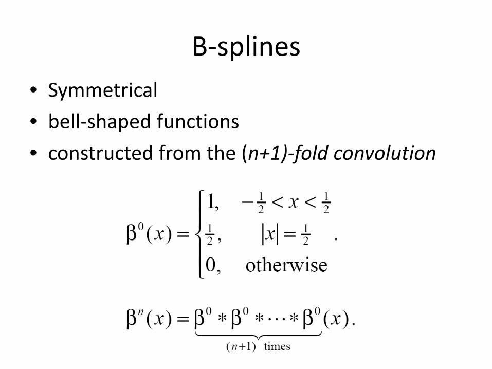
B‐splines• Symmetrical

• bell‐shaped functions

• constructed from the (n+1)‐fold convolution

B‐splines

B‐splines

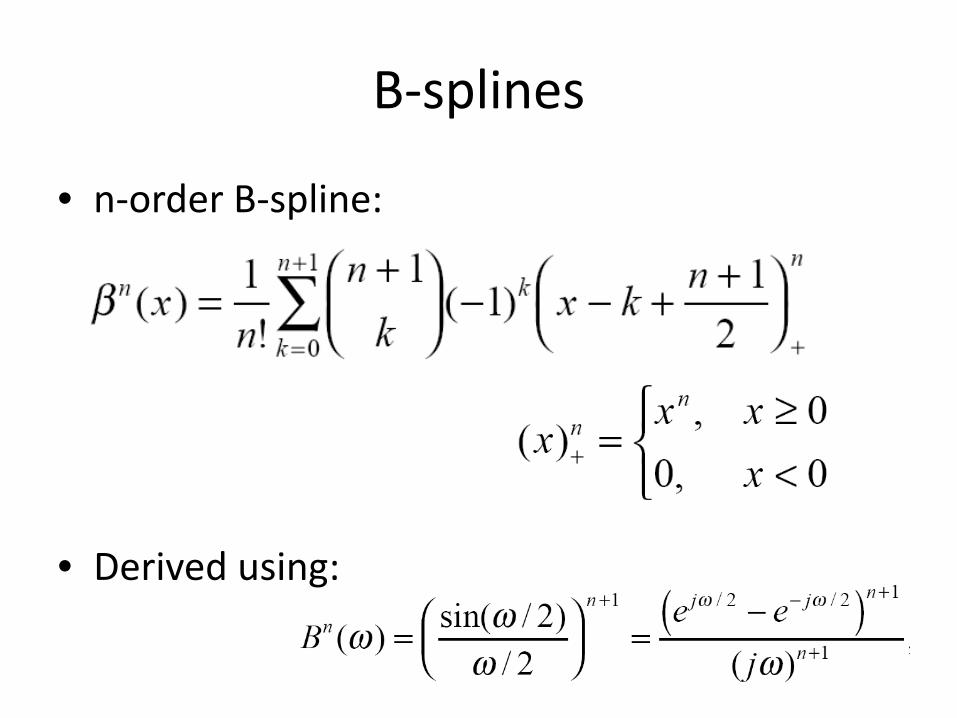
• n‐order B‐spline:

• Derived using:

B‐spline

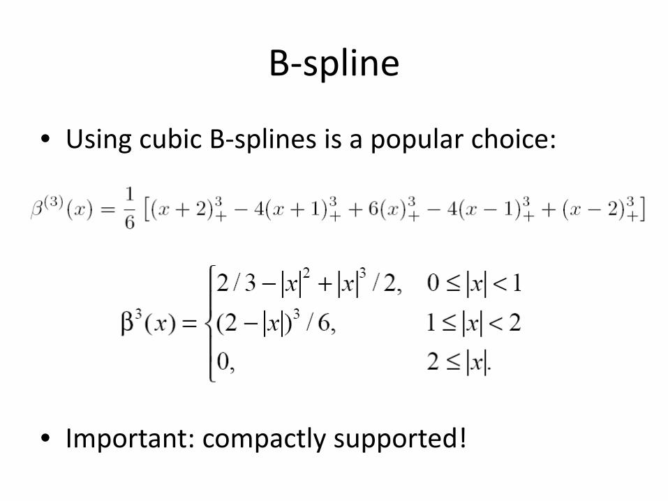
• Using cubic B‐splines is a popular choice:

• Important: compactly supported!

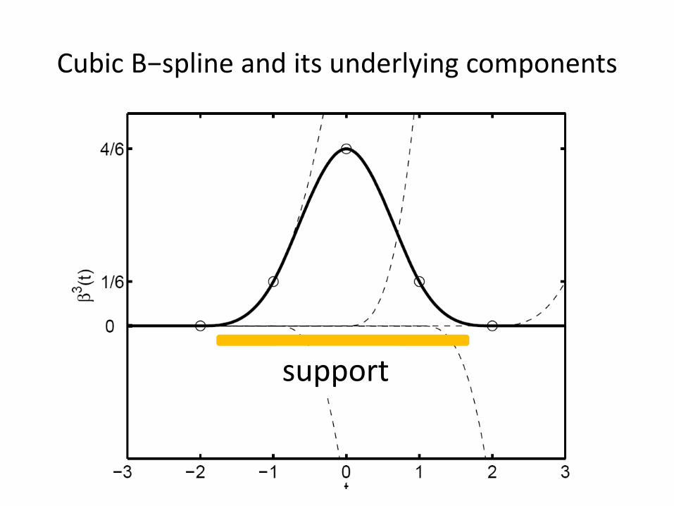
Cubic B−spline and its underlying components

support

B‐spline expansion 

Each spline is unambiguously characterized by its sequence of   B‐spline coefficients c(k)

Properties of B‐spline expansion 

• Discrete signal representation! (even though the underlying model is a continuous representation).

• Easy to manipulate; 

• E.g., derivatives:

B‐spline interpolation

• So far: B‐spline model of a given input signal s(x)

Interpolation problem: find coefficients c(k) such that spline function goes through the data points exactly

That is, reconstruct signal using a spline representation!

sd[n]

Reconstruct signal using a splinerepresentation

sd [n]

B‐spline interpolation

• Relationship between coefficients and samples

sd [n]

Obtained by sampling the B‐spline of degree n expanded by a factor of m (m=1)

= discrete B‐spline kernel

Cardinal B‐spline interpolation

Cardinal splines

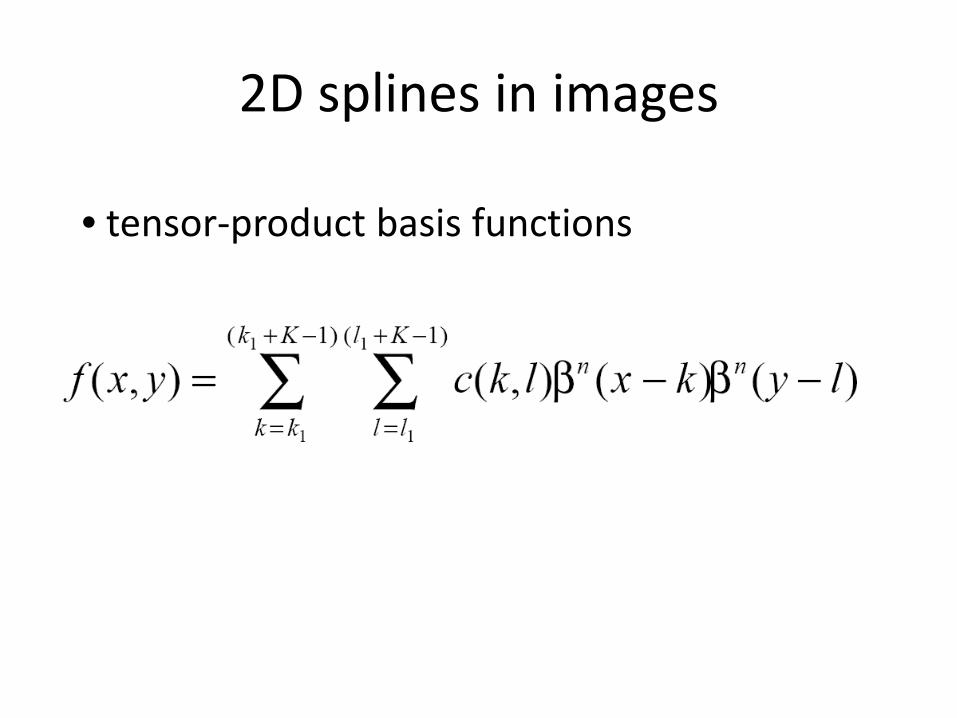
2D splines in images

• tensor‐product basis functions

B‐spline interpolation

• Conclusion:–n‐order differentiable

– Short spatial extent to minimize computation

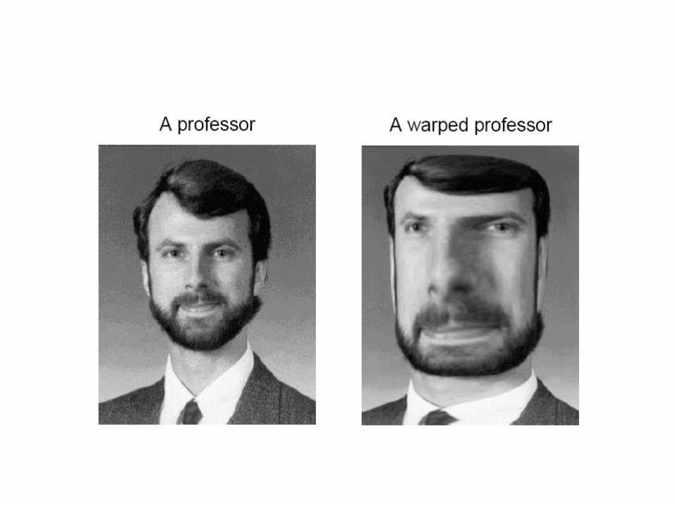
General image spatial transformations 

• transform the spatial coordinates of an image f(x, y) so that (after being transformed), it better “matches” another image– Ex: warping brain images into a standard coordinate system to facilitate automatic image analysis

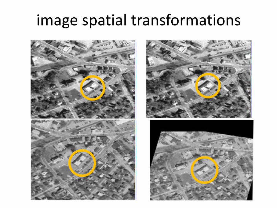
image spatial transformations

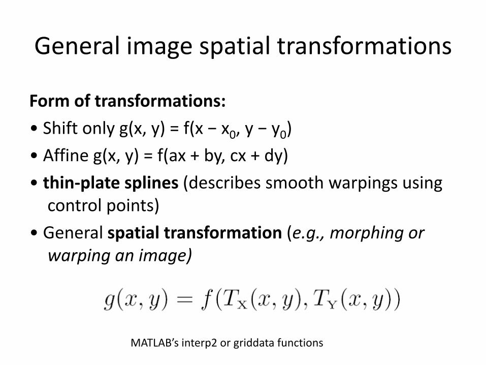
General image spatial transformations 

Form of transformations:

• Shift only g(x, y) = f(x − x0, y − y0)

• Affine g(x, y) = f(ax + by, cx + dy)

• thin‐plate splines (describes smooth warpings using control points)

• General spatial transformation (e.g., morphing or warping an image) 

MATLAB’s interp2 or griddata functions

Interpolation is critical!