Embed Size (px)
Citation preview

EECS 442 –
Computer vision
Face Recognition
• PCA (Eigen-faces)• LDA (Fisher-faces)• Boosting
Segments of this lectures are courtesy of Prof F. Li

Face Recognition•
Digital photography

Face Recognition•
Digital photography
•
Surveillance

Face Recognition•
Digital photography
•
Surveillance•
Album organization

Face Recognition•
Digital photography
•
Surveillance•
Album organization
•
Person tracking/id.

Face Recognition•
Digital photography
•
Surveillance•
Album organization
•
Person tracking/id.•
Emotions and expressions

Face Recognition•
Digital photography
•
Surveillance•
Album organization
•
Person tracking/id.•
Emotions and expressions
•
Security/warfare•
Tele-conferencing
•
Etc.

vs.
Identification
What’s ‘recognition’?

What’s ‘recognition’?
vs.
CategorizationIdentification

CategorizationIdentification
No
loca
lizat
ion
Yes, there are faces

CategorizationIdentification
No
loca
lizat
ionYes, there is John Lennon

CategorizationIdentification
No
loca
lizat
ion
Det
ectio
n or
Lo
caliz
atoi
n
John Lennon

CategorizationIdentification
No
loca
lizat
ion
Det
ectio
n or
Lo
caliz
atoi
n

What’s ‘recognition’?
CategorizationIdentification
No
loca
lizat
ion
Det
ectio
n or
Lo
caliz
atoi
n

CategorizationIdentification
No
loca
lizat
ion
1. PCA & Eigenfaces2. LDA & Fisherfaces
3. AdaBoost
4. Constellation modelDet
ectio
n or
Lo
caliz
atoi
n
Face Recognition methods

Eigenfaces
and Fishfaces
–
Principle Component Analysis (PCA)
–
Linear Discriminant
Analysis (LDA)
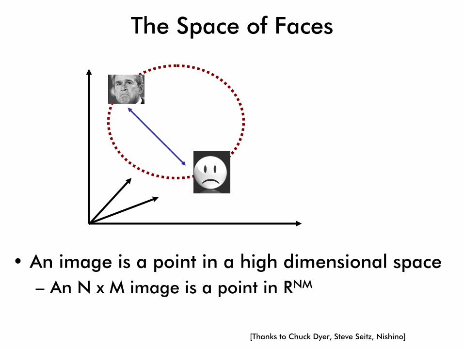
The Space of Faces
•
An image is a point in a high dimensional space–
An N x M image is a point in RNM
[Thanks to Chuck Dyer, Steve Seitz, Nishino]

• Images in the possible set are highly correlated.
• So, compress them to a low-dimensional subspace thatcaptures key appearance characteristics of the visual DOFs.
Key Idea
}x̂{=χ
• USE PCA for estimating the sub-space (dimensionality reduction)
•Compare two faces by projecting the images into the subspace and measuring the EUCLIDEAN distance between them.
EIGENFACES: [Turk and Pentland
91]

Image space
•
Computes p-dim subspace such that the projection of the data points onto the subspace has the largest variance
among all p-dim subspaces.
Face space
• Maximize the scatter
of the training images in face space

x1
x2
1 2
3
4
5
6
x1
x2
1 2
3
4
5
6
X1’
PCA projection
USE PCA for estimating the sub-space
•
Computes p-dim subspace such that the projection of the data points onto the subspace has the largest variance
among all p-dim subspaces.

x1
x2
1st principal component
2rd principal component
USE PCA for estimating the sub-space
Orthonormal
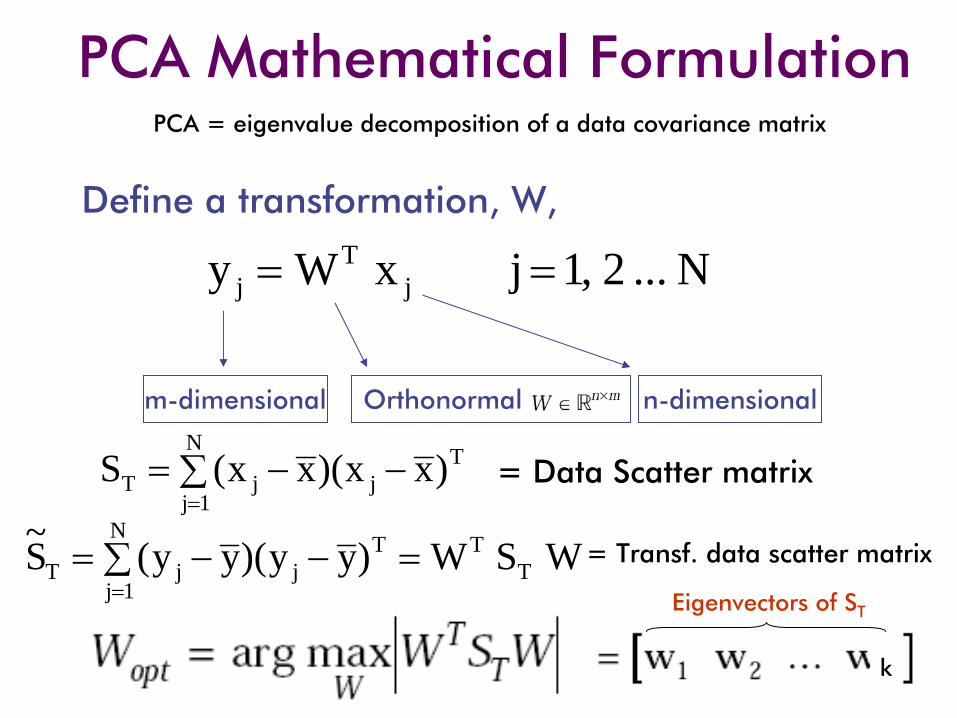
PCA Mathematical Formulation
Define a transformation, W,
m-dimensional n-dimensional
= Data Scatter matrixTj
N
1jjT )xx)(xx(S −−∑=
=
N...2,1jxWy jT
j ==
PCA = eigenvalue
decomposition of a data covariance matrix
= Transf. data scatter matrix
Eigenvectors of ST
k
WSW)yy)(yy(S~ TTT
j
N
1jjT =−−∑=
=
Eigenfaces
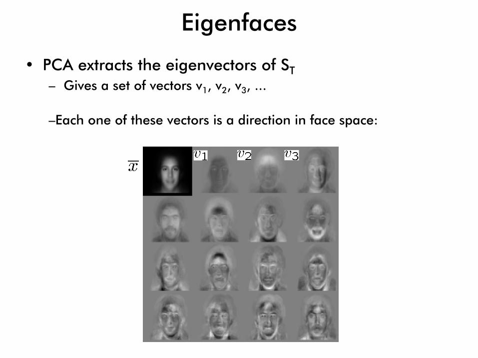
•
PCA extracts the eigenvectors of ST–
Gives a set of vectors v1
, v2
, v3
, ...
–Each one of these vectors is a direction in face space:

Projecting onto the Eigenfaces
•
The eigenfaces
v1
, ..., vK
span the space of faces
–
A face is converted to eigenface
coordinates by

Algorithm
1.
Align training images x1
, x2
, …, xN
2. Compute average face u = 1/N Σ
xi
3. Compute the difference image φi = xi – u
Training
Note that each image is formulated into a long vector!

Testing
1.
Projection in EigenfaceProjection ωi
= W (X –
u), W = {eigenfaces}
2. Compare projections
ST
= (1/N) Σ φi
φiT
= BBT, B=[φ1
, φ2
…
φN
]
4. Compute the covariance matrix (total scatter matrix)
5. Compute the eigenvectors of the covariance matrix , W
Algorithm
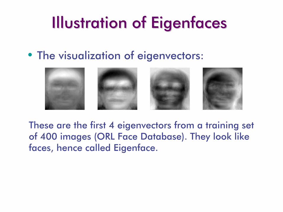
Illustration of Illustration of EigenfacesEigenfaces
These are the first 4 eigenvectors from a training set of 400 images (ORL Face Database). They look like faces, hence called Eigenface.
•
The visualization of eigenvectors:

Eigenfaces
look somewhat like generic faces.

•
Only selecting the top P eigenfaces reduces the dimensionality.
•
Fewer eigenfaces
result in more information loss, and
hence less discrimination between faces.
Reconstruction and ErrorsReconstruction and Errors
P = 4
P = 200
P = 400

EigenvaluesEigenvalues

Summary for Eigenface
Pros• Non-iterative, globally optimal solution
Limitations
•PCA projection is optimal for reconstruction from a low dimensional basis, but may NOT be
optimal for discrimination…

•
Global appearance method: not robust to misalignment, background variation
Limitations

Limitations
•
PCA assumes that the data has a Gaussian distribution (mean μ, covariance matrix Σ)
The shape of this dataset is not well described by its principal
componentsCredit slide: S. Lazebnik

PCA-SIFT: A More Distinctive Representation for Local Image Descriptors
-
Y Ke, R Sukthankar
-
IEEE CVPR 04
Extensions
•PCA-SIFT
•Generalized PCA: R. Vidal, Y. Ma, and S. Sastry. Generalized Principal Component Analysis (GPCA). IEEE Transactions on Pattern Analysis and Machine Intelligence, volume 27, number 12, pages 1 -
15, 2005.
•Tensor Faces:
"Multilinear
Analysis of Image Ensembles: TensorFaces," M.A.O. Vasilescu, D. Terzopoulos, Proc. 7th European Conference on Computer Vision (ECCV'02), Copenhagen, Denmark, May, 2002

Linear Discriminant Analysis (LDA) Fisher’s Linear Discriminant
(FLD)
•
Eigenfaces
attempt to maximise the scatter of the training images in face space
•
Fisherfaces
attempt to maximise the between class scatter, while minimising the within class scatter.

Illustration of the ProjectionIllustration of the Projection
Poor Projection
x1
x2
x1
x2
Using two classes as example:
Good

Comparing with PCAComparing with PCA

Variables
•
N Sample images: •
c classes:
•
Average of each class:
•
Total average:
{ }Nxx ,,1 L
{ }cχχ ,,1 L
∑=∈ ikx
ki
i xN χ
μ 1
∑==
N
kkx
N 1
1μ

Scatters
•
Scatter of class i: ( )( )Tikx
iki xxSik
μμχ
−∑ −=∈
∑==
c
iiW SS
1
( )( )∑ −−==
c
i
TiiiBS
1μμμμχ
BWT SSS +=
•
Within class scatter:
•
Between class scatter:
•
Total scatter:
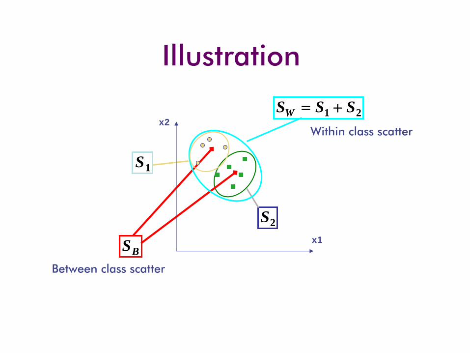
Illustration
2S
1S
BS
21 SSSW +=
x1
x2Within class scatter
Between class scatter

Mathematical Formulation (1)
•
After projection:
•
Between class scatter (of y’s):•
Within class scatter (of y’s):
kT
k xWy =
WSWS BT
B =~
WSWS WT
W =~

Illustration
2S
1S
BS
21 SSSW +=
x1
x2

Mathematical Formulation•
The desired projection:
WSW
WSW
SS
WW
TB
T
W
Bopt WW
max arg~~
max arg ==
miwSwS iWiiB ,,1 K== λ•
How is it found ? Generalized Eigenvectors
•
Data dimension is much larger than the number of samples
•
The matrix is singular:
Nn >>( ) cNSRank W −≤WS

Testing
1.
Projection in EigenfaceProjection ωi
= W opt (X –
u),
Wopt
= {fisher-faces}
2. Compare projections

Results: Eigenface
vs. Fisherface
(1)
• Variation in Facial Expression, Eyewear, and Lighting
•
Input: 160 images of 16 people
•
Train: 159 images
•
Test:
1 image
With glasses
Without glasses
3 Lighting conditions
5 expressions

Eigenface
vs. Fisherface
(2)

Face Recognition methods
CategorizationIdentification
No
loca
lizat
ion
Det
ectio
n or
Lo
caliz
atoi
n
1. PCA & Eigenfaces2. LDA & Fisherfaces
3. AdaBoost
4. Constellation model
Robust Face Detection Using AdaBoost
•
Brief intro on (Ada)Boosting•
Viola & Jones, 2001
Reference:P. Viola and M. Jones (2001) Robust Real-time Object Detection, IJCV.

Designing a strong classifier from a set of weak classifier
Features
Decision boundar
y
Computer screen
Background
In some feature space
Boosting

•
Defines a classifier using an additive model:
Boosting
Strong classifier
Weak classifier
WeightFeaturesvector

•
Defines a classifier using an additive model:
•
We need to define a family of weak classifiers
Boosting
Strong classifier
Weak classifier
WeightFeaturesvector
form a family of weak classifiers

•
A simple algorithm for learning robust classifiers–
Freund & Shapire, 1995
–
Friedman, Hastie, Tibshhirani, 1998
•
Provides efficient algorithm for sparse visual feature selection–
Tieu & Viola, 2000
–
Viola & Jones, 2003
•
Easy to implement, not requires external optimization tools.
Why boosting?

Linear classifiers•
Find linear function (hyperplane) to separate positive and negative examples
0:negative0:positive
<+⋅≥+⋅
bb
ii
ii
wxxwxx
Which hyperplane is best?
w, b

Support vector machines•
Find hyperplane
that maximizes the margin between
the positive and negative examples
1:1)(negative1:1)( positive−≤+⋅−=
≥+⋅=byby
iii
iii
wxxwxx
MarginSupport vectors
Distance between point and hyperplane: ||||
||wwx bi +⋅
For support, vectors, 1±=+⋅ bi wx
Therefore, the margin is 2 / ||w||
Credit slide: S. Lazebnik

• Datasets that are linearly separable work out great:
•
•
• But what if the dataset is just too hard?
• We can map it to a higher-dimensional space:
0 x
0 x
0 x
x2
Nonlinear SVMs
Slide credit: Andrew Moore

Φ: x →
φ(x)
Nonlinear SVMs
• General idea: the original input space can always be mapped to some higher-dimensional feature space where the training set is separable:
Slide credit: Andrew Moore
lifting transformation

Each data point has
a class label:
wt =1and a weight:
+1 ( )
-1 ( )yt
=
Boosting
•
It is a sequential procedure:
xt=1
xt=2
xt
Y. Freund and R. Schapire, A short introduction to boosting, Journal of Japanese Society for Artificial Intelligence, 14(5):771-780, September, 1999.

Toy exampleWeak learners from the family of lines
h => p(error) = 0.5 it is at chance
Each data point has
a class label:
wt =1and a weight:
+1 ( )
-1 ( )yt
=

Toy example
This one seems to be the best
This is a ‘weak classifier’: It performs slightly better than chance.
Each data point has
a class label:
wt =1and a weight:
+1 ( )
-1 ( )yt
=
Toy example
Each data point has
a class label:
wt wt
exp{-yt
Ht
}
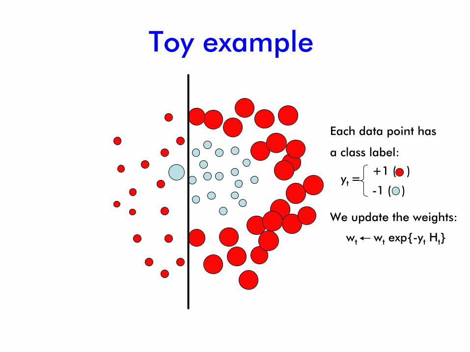
We update the weights:
+1 ( )
-1 ( )yt
=

Toy example
Each data point has
a class label:
wt wt
exp{-yt
Ht
}
We update the weights:
+1 ( )
-1 ( )yt
=

Toy example
Each data point has
a class label:
wt wt
exp{-yt
Ht
}
We update the weights:
+1 ( )
-1 ( )yt
=

Toy example
Each data point has
a class label:
wt wt
exp{-yt
Ht
}
We update the weights:
+1 ( )
-1 ( )yt
=

Toy example
The strong (non-
linear) classifier is built as the combination of all the weak (linear) classifiers.
f1 f2
f3
f4

The Viola/Jones Face Detector
•
A “paradigmatic”
method for real-time object detection
•
Training is slow, but detection is very fast•
Key ideas–
Integral images for fast feature evaluation
–
Boosting for feature selection–
Attentional cascade for fast rejection of non-
face windows
P. Viola and M. Jones. Rapid object detection using a boosted cascade of simple features. CVPR 2001.
Credit slide: S. Lazebnik

Feature selection
Discriminative featuresNon discriminative features

Image Features
•4 kind of Rectangle filters
•Value =
∑
(pixels in white area) – ∑
(pixels in black area)
Credit slide: S. Lazebnik

ExampleSource
Result
Credit slide: S. Lazebnik

Fast computation with integral images
•
The integral image computes a value at each pixel (x,y ) that is the sum of the pixel values above and to the left of (x,y ), inclusive
•
This can quickly be computed in one pass through the image
(x,y)
,( , ) ( , )
x x y yii x y i x y
′ ′≤ ≤
′ ′= ∑
Credit slide: S. Lazebnik

Computing sum within a rectangle
•
Let A,B,C,D be the values of the integral image at the corners of a rectangle
Fast computation with integral images
•Only 3 additions are required for any size of rectangle!
–This is now used in many areas of computer vision–E.g. Histogram of features in rectangular areas
•Then the sum of original image values within the rectangle can be computed as:
sum = A – B – C + D
D B
C A
Credit slide: S. Lazebnik

Feature selection
•
For a 24x24 detection region, the number of possible rectangle features is ~180,000!
Credit slide: S. Lazebnik

Feature selection
•
For a 24x24 detection region, the number of possible rectangle features is ~180,000!
•
At test time, it is impractical to evaluate the entire feature set
•
Can we create a good classifier using just a small subset of all possible features?
•
How to select such a subset?
Credit slide: S. Lazebnik

•
Boosting combines weak learners into a more accurate ensemble classifier
•
Weak learner: classifier with accuracy that need be only better than chance
•
We can define weak learners based on rectangle features:
window
value of rectangle feature
threshold
1 if ( )( )
0 otherwisej j
j
f xh x
θ>⎧= ⎨⎩
Boosting for face detection

• For each round of boosting:
1.
Evaluate each rectangle filter on each example
2.
Select best filter/threshold combination
3.
Reweight examples
Boosting for face detection

…..
1( ,1)x 2( ,1)x 3( ,0)x 4( ,0)x
( , )n nx y1α
5( ,0)x 6( ,0)x
Weak classifier
threshold
1 if ( )( )
0 otherwisej j
j
f xh x
θ>⎧= ⎨⎩
1. Evaluate each rectangle filter on each example
Boosting for face detection

b.
For each feature, j ( )j i j i iiw h x yε = −∑
1 if ( )( )
0 otherwisej j
j
f xh x
θ>⎧= ⎨⎩
c.
Choose the classifier, ht
with the lowest error tε
1 ( )1, ,
t i ih x yt i t i tw w β − −+ =
1t
tt
εβε
=−
Boosting for face detection
2. Select best filter/threshold combination
,,
,1
t it i n
t jj
ww
w=
←∑a.
Normalize the weights
3. Reweight examples

4. The final strong classifier is
1 1
11 ( )( ) 2
0 otherwise
T Tt t tt th x
h xα α
= =
⎧ ≥⎪= ⎨⎪⎩
∑ ∑1logt
t
αβ
=
Boosting for face detection
The final hypothesis is a weighted linear combination of the T hypotheses where the weights are inversely proportional to the training errors

First two features selected by boosting

Cascading classifiers•
We start with simple classifiers which reject many of the negative sub-windows while detecting almost all positive sub-windows
•
Positive results from the first classifier triggers the evaluation of a second (more complex) classifier, and so on
•
A negative outcome at any point leads to the immediate rejection of the sub-window
FACEIMAGESUB-WINDOW
Classifier 1T
Classifier 3T
F
NON-FACE
TClassifier 2
T
F
NON-FACE
F
NON-FACECredit slide: S. Lazebnik

Cascading classifiers•
Chain classifiers that are progressively more complex and have lower false positive rates:
vs false negdetermined by
% False Pos
% D
etec
tion
0 50
50
100
FACEIMAGESUB-WINDOW
Classifier 1T
Classifier 3T
F
NON-FACE
TClassifier 2
T
F
NON-FACE
F
NON-FACE
Receiver operating characteristic
Credit slide: S. Lazebnik

Training the cascade•
Adjust weak learner threshold to minimize false negatives (as opposed to total classification error)
•
Each classifier trained on false positives of previous stages–
A single-feature classifier achieves 100% detection rate and about 50% false positive rate
–
A five-feature classifier achieves 100% detection rate and 40% false positive rate (20% cumulative)
–
A 20-feature classifier achieve 100% detection rate with 10% false positive rate (2% cumulative)
1 Feature 5 Features
F
50%20 Features
20% 2%FACE
NON-FACE
F
NON-FACE
F
NON-FACE
IMAGESUB-WINDOW
Credit slide: S. Lazebnik

The implemented system•
Training Data–
5000 faces•
All frontal, rescaled to 24x24 pixels
–
300 million
non-faces•
9500 non-face images
–
Faces are normalized•
Scale, translation
•
Many variations–
Across individuals–
Illumination–
Pose
(Most slides from Paul Viola)

System performance
•
Training time: “weeks”
on 466 MHz Sun workstation
•
38 layers, total of 6061 features
•
Average of 10 features evaluated per window on test set
•
“On a 700 Mhz
Pentium III processor, the face detector
can process a 384 by 288 pixel image in about .067 seconds”–
15 Hz–
15 times faster than previous detector of comparable accuracy (Rowley et al., 1998)

Output of Face Detector on Test Images

Other detection tasks
Facial Feature Localization
Male vs. female
Profile Detection

Profile Detection

Profile Features

Face Image Databases
•
Databases for face recognition can be best utilized as training sets–
Each image consists of an individual on a uniform and uncluttered background
•
Test Sets for face detection–
MIT, CMU (frontal, profile), Kodak

Experimental Results
•
Test dataset–
MIT+CMU frontal face test set
–
130 images with 507 labeled frontal faces
MIT test set: 23 images with 149 facesSung & poggio: detection rate 79.9% with 5 false positiveAdaBoost: detection rate 77.8% with 5 false positives
False detection
10 31 50 65 78 95 110 167 422
AdaBoost 78.3 85.2 88.8 89.8 90.1 90.8 91.1 91.8 93.7
Neural-net 83.2 86.0 - - - 89.2 - 90.1 89.9

Experimental Results
-> not significantly different accuracy
-> but the cascade class. almost 10 times faster

Summary: Viola/Jones detector
•
Rectangle features
•
Integral images for fast computation
•
Boosting for feature selection
•
Attentional
cascade for fast rejection of negative
windows

Sharing features with Boosting
Matlab
code
• Gentle boosting
•
Object detector using a part based model
http://people.csail.mit.edu/torralba/iccv2005/
Sharing features: efficient boosting procedures for multiclass object detection
A. Torralba, K. P. Murphy and W. T. Freeman Proceedings of the IEEE Computer Society Conference on Computer Vision and Pattern Recognition (CVPR). pp 762-769, 2004.

Next lecture
Optical flow and tracking