EECS 369: Introduction to Sensor

Networks

Winter 2011

Instructors:

Peter Scheuermann and Goce Trajcevski

1

2

Part 3: Self-Configuration

3.1. Time Synchronization

3.2. Localization

VI-3

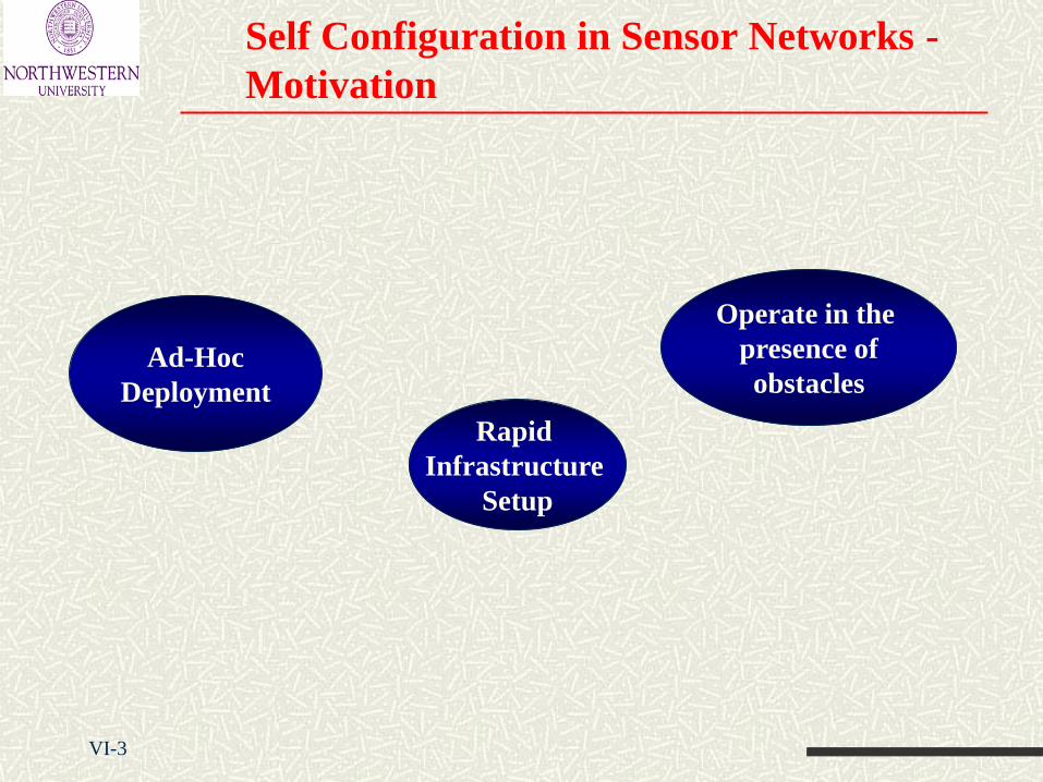
Self Configuration in Sensor Networks -

Motivation

Operate in the

presence of

obstacles

Rapid

Infrastructure

Setup

Ad-Hoc

Deployment

Self-configuration Challenges

1. Timing synchronization

When did an event take place?

2. Node Localization

Where did an event take place?

3. Calibration

What is the value of an event?

Self-configuration crucial to relate to the physical world!

4

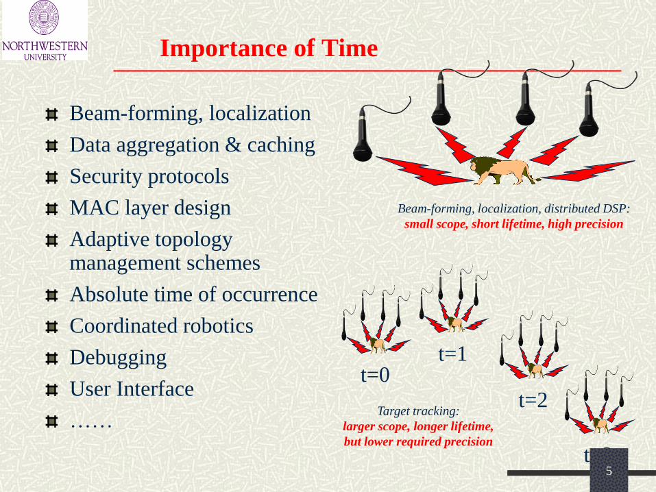
Importance of Time

Beam-forming, localization

Data aggregation & caching

Security protocols

MAC layer design

Adaptive topology management schemes

Absolute time of occurrence

Coordinated robotics

Debugging

User Interface

……

t=0 t=1

t=2

t=3

Beam-forming, localization, distributed DSP:

small scope, short lifetime, high precision

Target tracking:

larger scope, longer lifetime,

but lower required precision

5

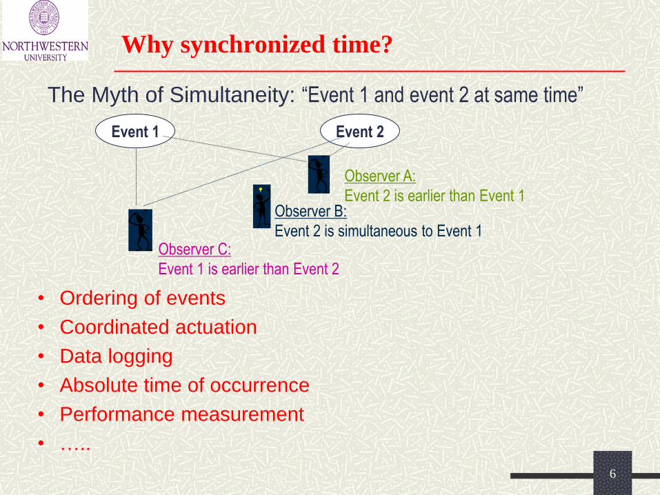
Why synchronized time?

The Myth of Simultaneity: “Event 1 and event 2 at same time”

Event 1 Event 2

Observer A:

Event 2 is earlier than Event 1 Observer B:

Event 2 is simultaneous to Event 1 Observer C:

Event 1 is earlier than Event 2

• Ordering of events

• Coordinated actuation

• Data logging

• Absolute time of occurrence

• Performance measurement

• …..

6

Time Synchronization Quality Metrics

Maximum Error

Lifetime

Scope & Availability

Efficiency (use of power and time)

Cost and form factor

…

7

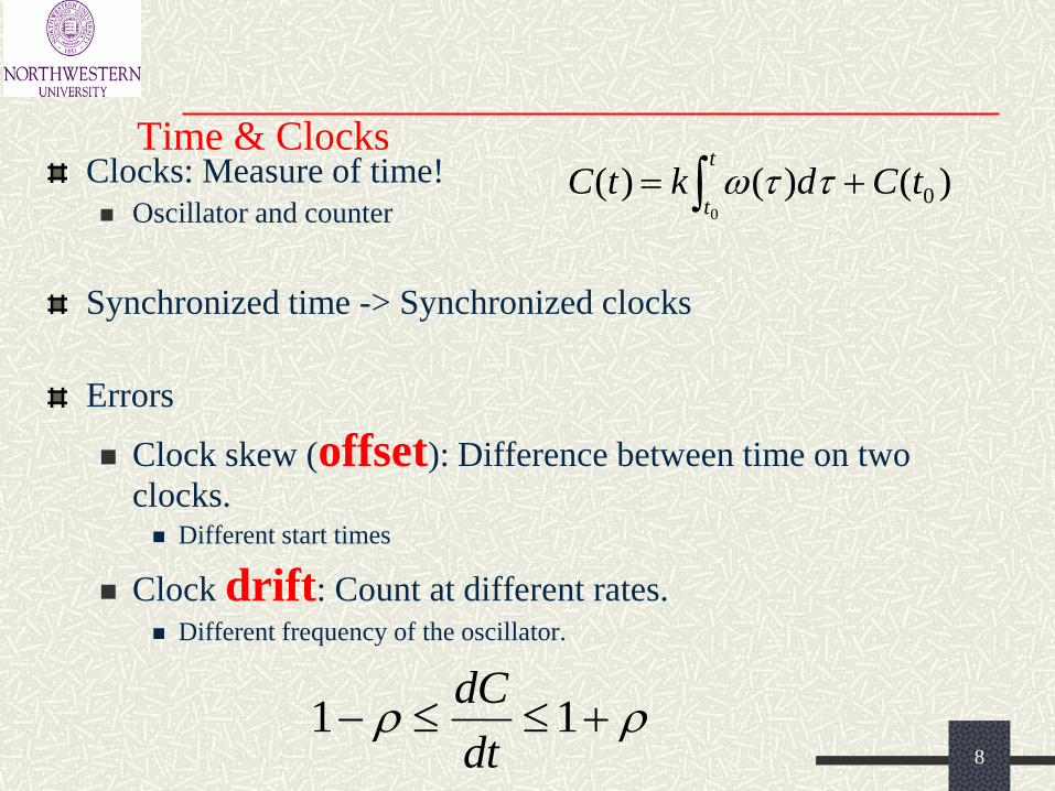
Time & Clocks Clocks: Measure of time!

Oscillator and counter

Synchronized time -> Synchronized clocks

Errors

Clock skew (offset): Difference between time on two

clocks. Different start times

Clock drift: Count at different rates. Different frequency of the oscillator.

t

ttCdktC

0

)()()( 0

11dt

dC

8

VI-9

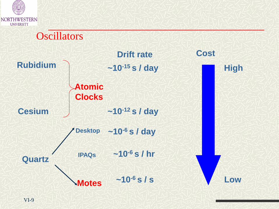
Oscillators

Rubidium

Cesium

Quartz

Drift rate Cost

~10-15 s / day

~10-12 s / day

~10-6 s / day

High

Low ~10-6 s / s

~10-6 s / hr

Desktop

IPAQs

Atomic

Clocks

Motes

VI-10

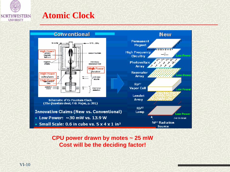
Atomic Clock

CPU power drawn by motes ~ 25 mW

Cost will be the deciding factor!

Time

e31

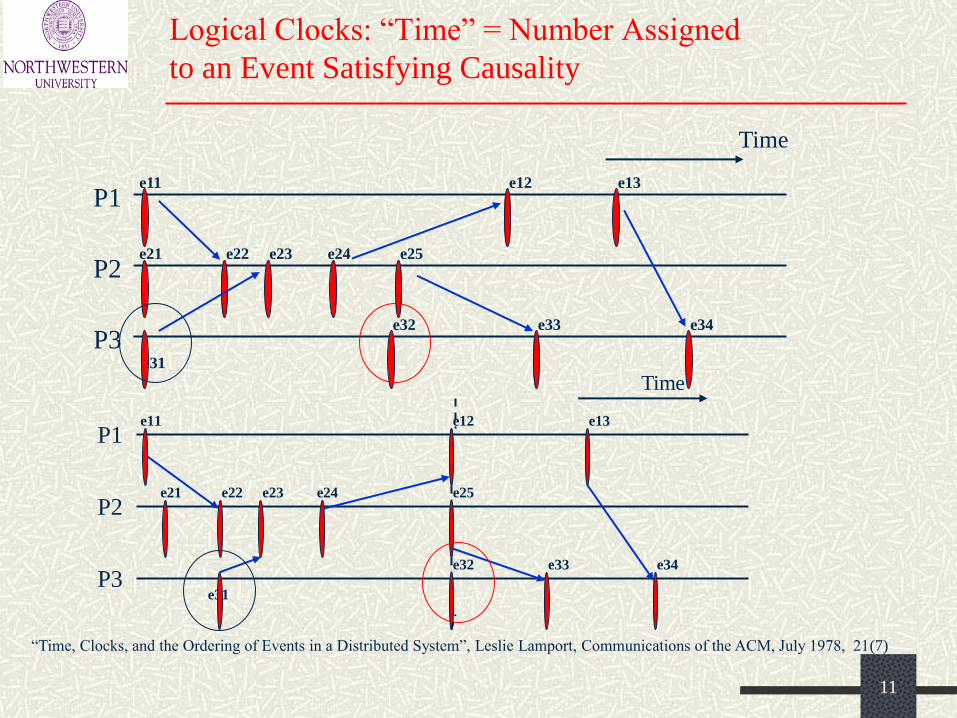
Logical Clocks: “Time” = Number Assigned

to an Event Satisfying Causality

P2

P1

P3

e21

e11

e22 e23 e24 e25

e12 e13

e32 e33 e34

P2

P1

P3

Time

e21

e31

e11

e22 e23 e24 e25

e12 e13

e32 e33 e34

“Time, Clocks, and the Ordering of Events in a Distributed System”, Leslie Lamport, Communications of the ACM, July 1978, 21(7)

11

Implementing Logical Clock

With synchronized physical clocks

An event a happened before an event b if a happened at an earlier time than b

Without physical clocks:

Happened before relation “”

If a and b are events in the same node, and a comes before b, then ab

If a is the sending of a packet by one node and b is the receipt of the same message by another node, then ab

If ab and bc, then ac

Local clock Ci for each node Ni

Assigns a number Ci(a) to any event at a node

Each node Ni increments Ci between any two successive events

Ensures event ordering within a node

(a) if event a is the sending of a message m by node Ni, then the message m contains a timestamp Tm = Ci(a), and

(b) Upon receiving a message m, node Nj sets Cj greater than or equal to its present value and greater than Tm

Ensures event ordering across nodes

Using this method, one can assign a unique timestamp to each event in a distributed system to provide a total ordering of all events

But not enough for many applications! 12

Technologies for Absolute Time

Synchronization

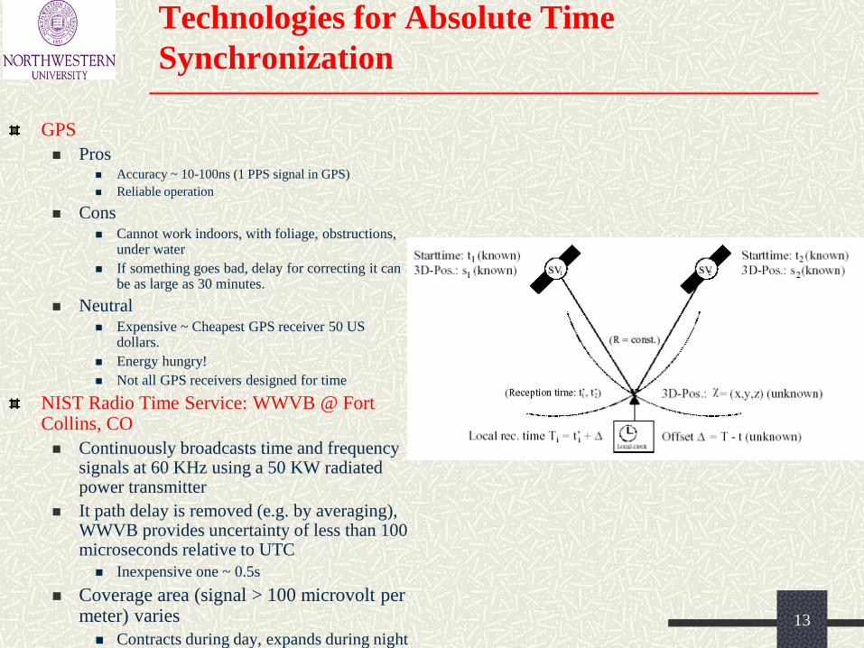
GPS

Pros Accuracy ~ 10-100ns (1 PPS signal in GPS)

Reliable operation

Cons Cannot work indoors, with foliage, obstructions,

under water

If something goes bad, delay for correcting it can be as large as 30 minutes.

Neutral Expensive ~ Cheapest GPS receiver 50 US

dollars.

Energy hungry!

Not all GPS receivers designed for time

NIST Radio Time Service: WWVB @ Fort Collins, CO

Continuously broadcasts time and frequency signals at 60 KHz using a 50 KW radiated power transmitter

It path delay is removed (e.g. by averaging), WWVB provides uncertainty of less than 100 microseconds relative to UTC

Inexpensive one ~ 0.5s

Coverage area (signal > 100 microvolt per meter) varies

Contracts during day, expands during night 13

Why not put a GPS receiver at every

sensor node?

Outages:

GPS: foliage etc.

WWVB: typically available for ~ 20 hours/day

Other 4 hours you are stuck with an uncompensated clock oscillator

Accuracy

Inexpensive receivers don’t give good accuracies: intermittent

synchronization, serial port delay and jitter

Listening on a radio is not cheap - energy!!!

14

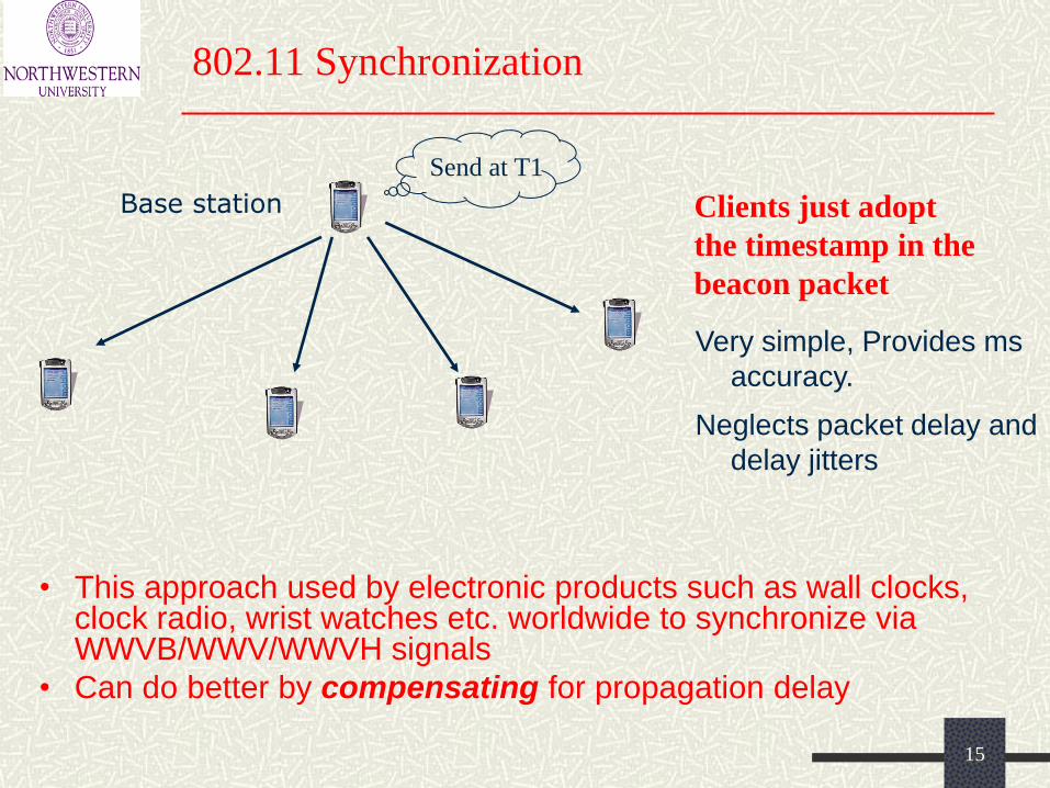
802.11 Synchronization

Clients just adopt

the timestamp in the

beacon packet

Send at T1

Base station

Very simple, Provides ms

accuracy.

Neglects packet delay and

delay jitters

• This approach used by electronic products such as wall clocks, clock radio, wrist watches etc. worldwide to synchronize via WWVB/WWV/WWVH signals

• Can do better by compensating for propagation delay

15

VI-16

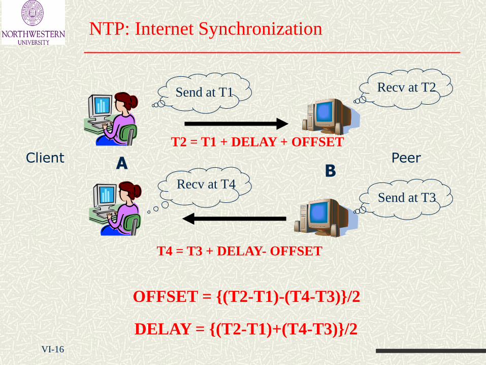
NTP: Internet Synchronization

A

Send at T3 Recv at T4

T4 = T3 + DELAY- OFFSET

Send at T1 Recv at T2

T2 = T1 + DELAY + OFFSET

B

OFFSET = {(T2-T1)-(T4-T3)}/2

DELAY = {(T2-T1)+(T4-T3)}/2

Client Peer

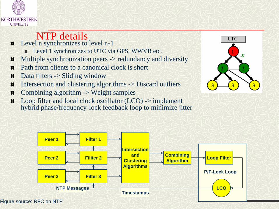
NTP details Level n synchronizes to level n-1 Level 1 synchronizes to UTC via GPS, WWVB etc.

Multiple synchronization peers -> redundancy and diversity

Path from clients to a canonical clock is short

Data filters -> Sliding window

Intersection and clustering algorithms -> Discard outliers

Combining algorithm -> Weight samples

Loop filter and local clock oscillator (LCO) -> implement hybrid phase/frequency-lock feedback loop to minimize jitter

NTP Messages

Peer 1

Peer 2

Filter 1

Peer 3

Filiter 2

Filter 3

Intersection

and

Clustering

Algorithms

Combining

Algorithm Loop Filter

LCO Timestamps

P/F-Lock Loop

Figure source: RFC on NTP

NTP Evaluation

• Pros

– Readily available

– Industry standard

– Achieves secure and stable sync to ms accuracy

• Cons

– Designed for ms accuracy only!

– Not flexible

– Impact of poor topologies

– Designed for constant operation in the background at low rates

• E.g. it took NTP an hour to reduce error to 60 microseconds with

maximum polling rate of 16 sec.

• Neutral

– Not energy friendly! 18

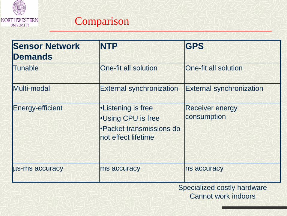
Comparison

Sensor Network

Demands

NTP GPS

Tunable One-fit all solution One-fit all solution

Multi-modal External synchronization External synchronization

Energy-efficient •Listening is free

•Using CPU is free

•Packet transmissions do

not effect lifetime

Receiver energy

consumption

µs-ms accuracy ms accuracy ns accuracy

Specialized costly hardware

Cannot work indoors

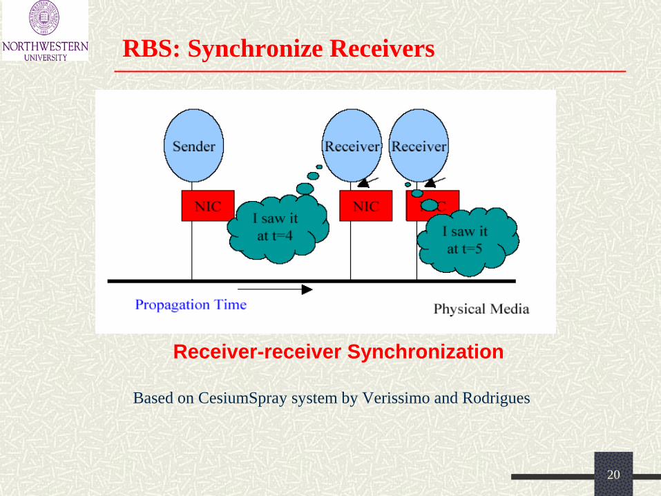
RBS: Synchronize Receivers

Based on CesiumSpray system by Verissimo and Rodrigues

Receiver-receiver Synchronization

20

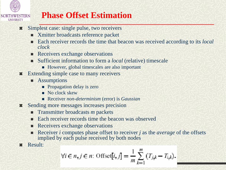
Phase Offset Estimation

Simplest case: single pulse, two receivers

Xmitter broadcasts reference packet

Each receiver records the time that beacon was received according to its local clock

Receivers exchange observations

Sufficient information to form a local (relative) timescale However, global timescales are also important

Extending simple case to many receivers

Assumptions Propagation delay is zero

No clock skew

Receiver non-determinism (error) is Gaussian

Sending more messages increases precision

Transmitter broadcasts m packets

Each receiver records time the beacon was observed

Receivers exchange observations

Receiver i computes phase offset to receiver j as the average of the offsets implied by each pulse received by both nodes

Result:

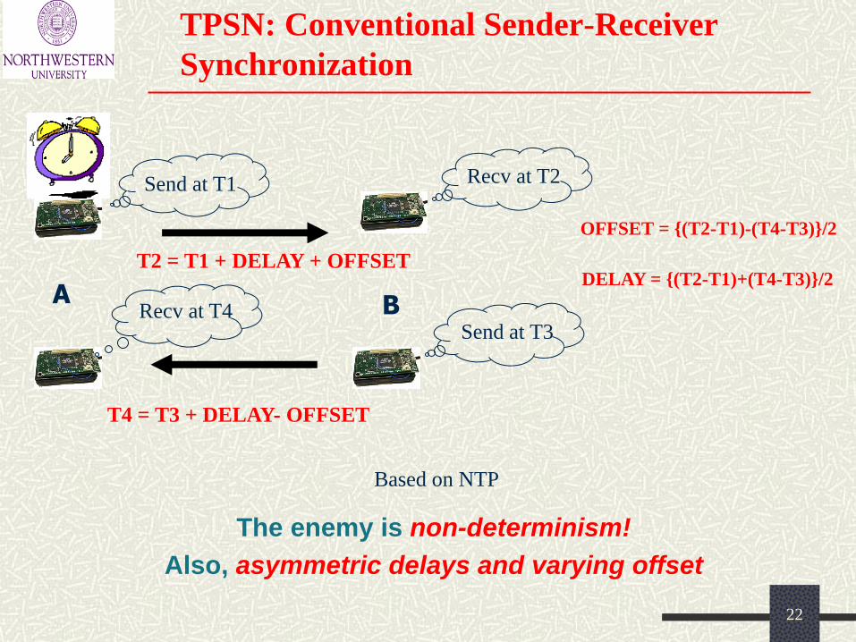
TPSN: Conventional Sender-Receiver

Synchronization

A

Send at T3 Recv at T4

T4 = T3 + DELAY- OFFSET

Send at T1 Recv at T2

T2 = T1 + DELAY + OFFSET

B

OFFSET = {(T2-T1)-(T4-T3)}/2

DELAY = {(T2-T1)+(T4-T3)}/2

Based on NTP

The enemy is non-determinism!

Also, asymmetric delays and varying offset

22

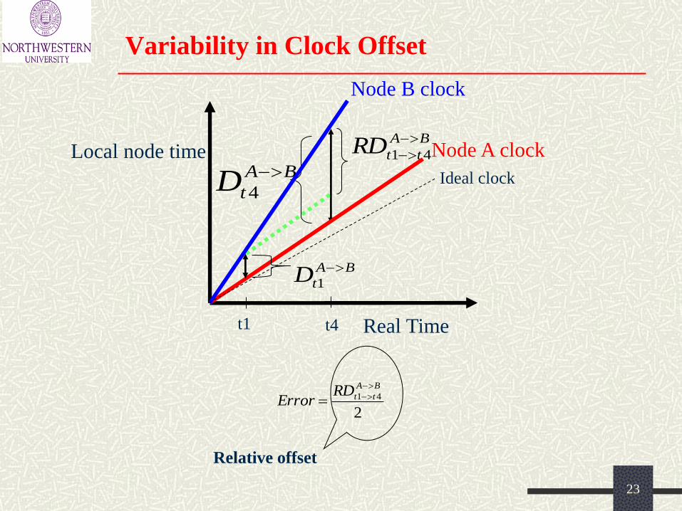
Variability in Clock Offset

BA

ttRD

41

t4

BA

tD

4

Real Time

Ideal clock

Node B clock

Node A clock

t1

BA

tD

1

Local node time

Relative offset

2

41

BA

ttRDError

23

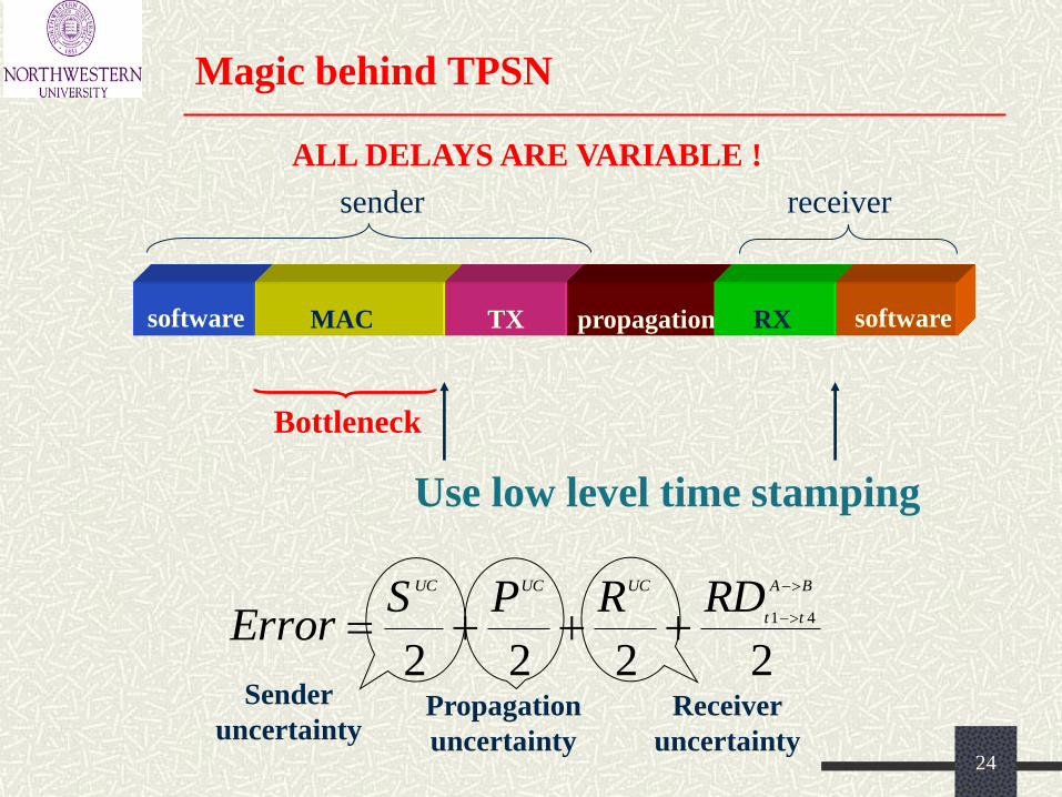
Magic behind TPSN

ALL DELAYS ARE VARIABLE !

software MAC propagation TX RX software

sender receiver

Bottleneck

Use low level time stamping

Sender

uncertainty Propagation

uncertainty

Receiver

uncertainty

2222

41

BA

tt

UCUCUC RDRPSError

24

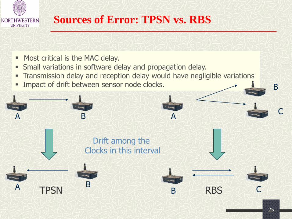
Sources of Error: TPSN vs. RBS

Most critical is the MAC delay.

Small variations in software delay and propagation delay. Transmission delay and reception delay would have negligible variations Impact of drift between sensor node clocks.

A

B

B

A

B

A C

B C

Drift among the Clocks in this interval

TPSN RBS

25

A

B

H

E

C F

K

D G

L

J I

0 1

2

3

1

1

1

2

2

2 2 3

Levels now

all assigned

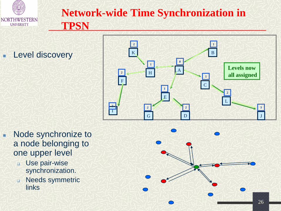
Network-wide Time Synchronization in

TPSN

Level discovery

Node synchronize to a node belonging to one upper level Use pair-wise

synchronization.

Needs symmetric links

26

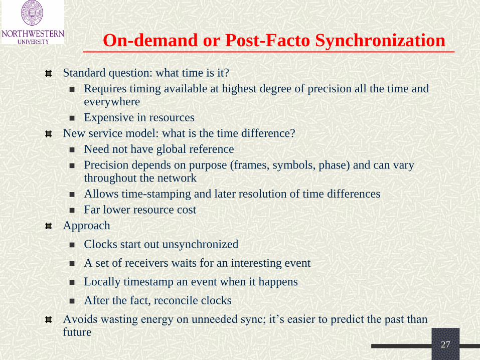
On-demand or Post-Facto Synchronization

Standard question: what time is it?

Requires timing available at highest degree of precision all the time and everywhere

Expensive in resources

New service model: what is the time difference?

Need not have global reference

Precision depends on purpose (frames, symbols, phase) and can vary throughout the network

Allows time-stamping and later resolution of time differences

Far lower resource cost

Approach

Clocks start out unsynchronized

A set of receivers waits for an interesting event

Locally timestamp an event when it happens

After the fact, reconcile clocks

Avoids wasting energy on unneeded sync; it’s easier to predict the past than future

27

VI-28

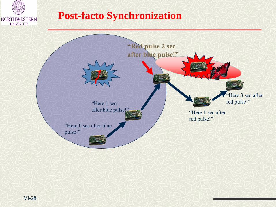
Post-facto Synchronization

“Here 3 sec after

red pulse!”

“Here 0 sec after blue

pulse!”

“Here 1 sec

after blue pulse!” “Here 1 sec after

red pulse!”

“Red pulse 2 sec

after blue pulse!”

VI-29

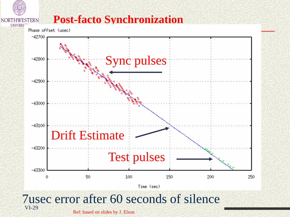
Post-facto Synchronization

Test pulses

Sync pulses

Drift Estimate

7usec error after 60 seconds of silence Ref: based on slides by J. Elson

1

3

2

A

4

8

C

5

7

6 B

10

D

11

9

1 3

2

4

8

5 7

6

10

11

9

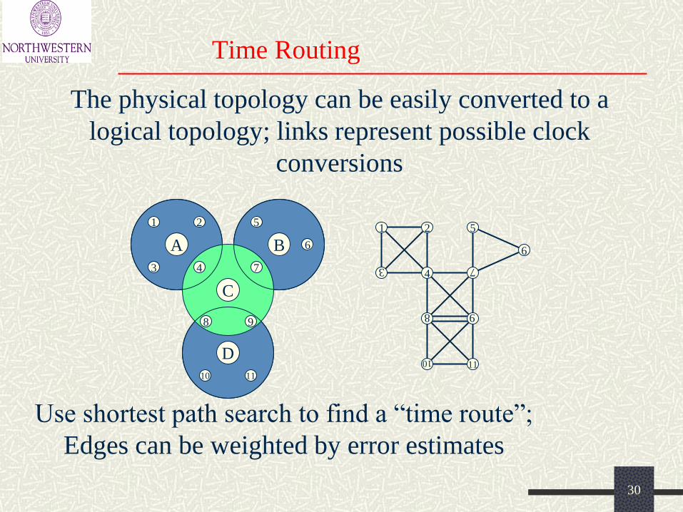
Time Routing

The physical topology can be easily converted to a

logical topology; links represent possible clock

conversions

Use shortest path search to find a “time route”;

Edges can be weighted by error estimates

30

Synchronizing to External Standards

1

3

2

A

4

8

C

5

7

6 B

10

D

9

1

3

2

4

8

5

7

6

10 11

9

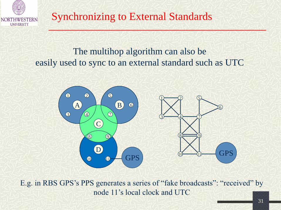
The multihop algorithm can also be

easily used to sync to an external standard such as UTC

GPS 11 GPS

E.g. in RBS GPS’s PPS generates a series of “fake broadcasts”: “received” by

node 11’s local clock and UTC 31

32

Localization - Motivation

• Track items (boxes in a warehouse, badges in a building, etc)

• Identify items (the thermostat in the corner office)

• Not everything needs an IP address

• Cost and Physical Environment

• Energy Efficiency

Well, GPS does not work everywhere

• Smart Systems – devices need to know where they are

• Geographic routing & coverage problems

• People and asset tracking

Sensor’s reading is too hot!!! WHERE???

33

Localization - Challenges

Physical Layer Measurement Challenges:

Multipath, shadowing, sensor imperfections, changes in

propagation properties and more

Computational Challenges

* Many formulations of localization problems:

(e.g., how to solve the optimization problem, distributed

solution)

Plus:

May not have base stations or beacons for relative positioning

GPS may not be available

Sensor nodes may fail

Low-end sensor nodes

34

Localization Techniques

1. Electromagnetic Trackers:

High accuracy and resolution, but VERY expensive

2. Optical Trackers (Gyroscope):

Robust, high accuracy and resolution, expensive and mechanically complex; calibration needed.

3. Radio Position Systems (such as GPS):

Successful in the wide area, but ineffective in buildings, only

offer modest location accuracy; cost, size and unavailability.

4. GPS-less Techniques

a) Beacon Based Techniques

b) Relative Location Based Techniques

35

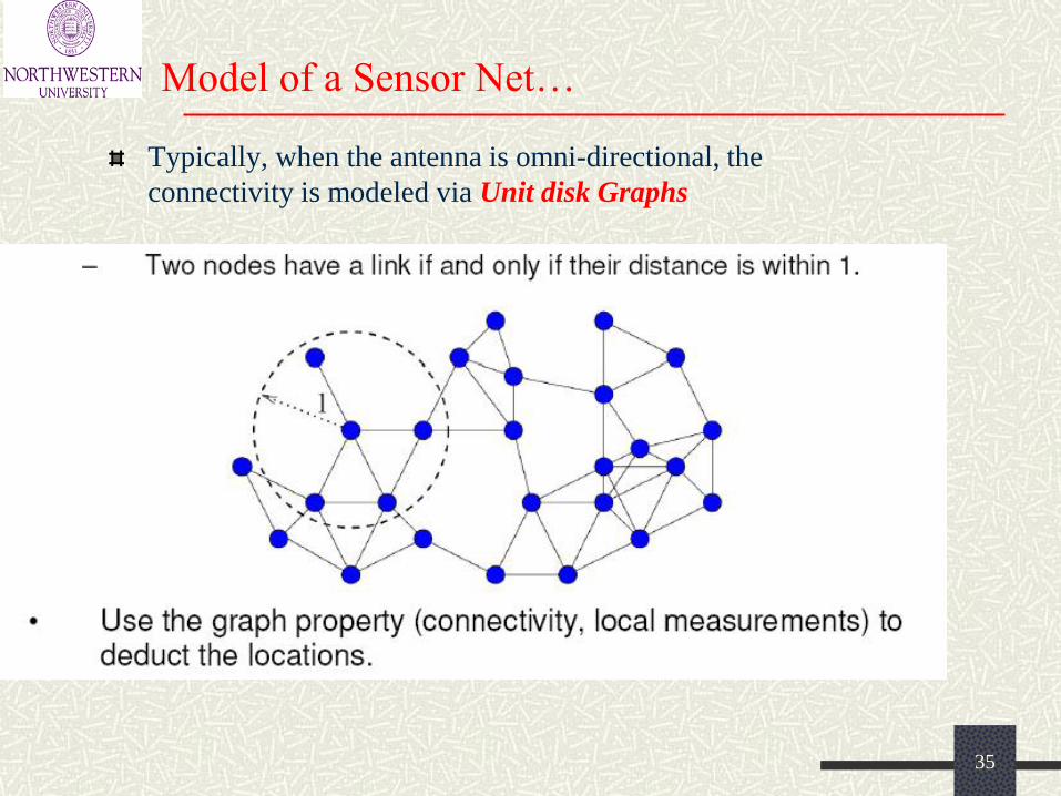
Model of a Sensor Net…

Typically, when the antenna is omni-directional, the

connectivity is modeled via Unit disk Graphs

36

Some Basic Concepts…

• Output: nodes’ location.

– Global location, e.g., what GPS gives.

– Relative location.

• Input:

– Connectivity, hop count.

• Nodes with k hops away are within Euclidean distance k.

• Nodes without a link must be at least distance 1 away.

– Distance measurement of an incoming link.

– Angle measurement of an incoming link.

– Combinations of the above.

37

Categorization of Localization Approaches

Given distances or angle measurements, find the locations of

the sensors.

• Anchor-based

– Some nodes know their locations, either by a GPS or as

prespecified.

• Anchor-free

– Relative location only.

– A harder problem, need to solve the global structure. Nowhere to

start.

• Range-based

– Use range information (distance estimation).

• Range-free

– No distance estimation, use connectivity information such as hop

count.

38

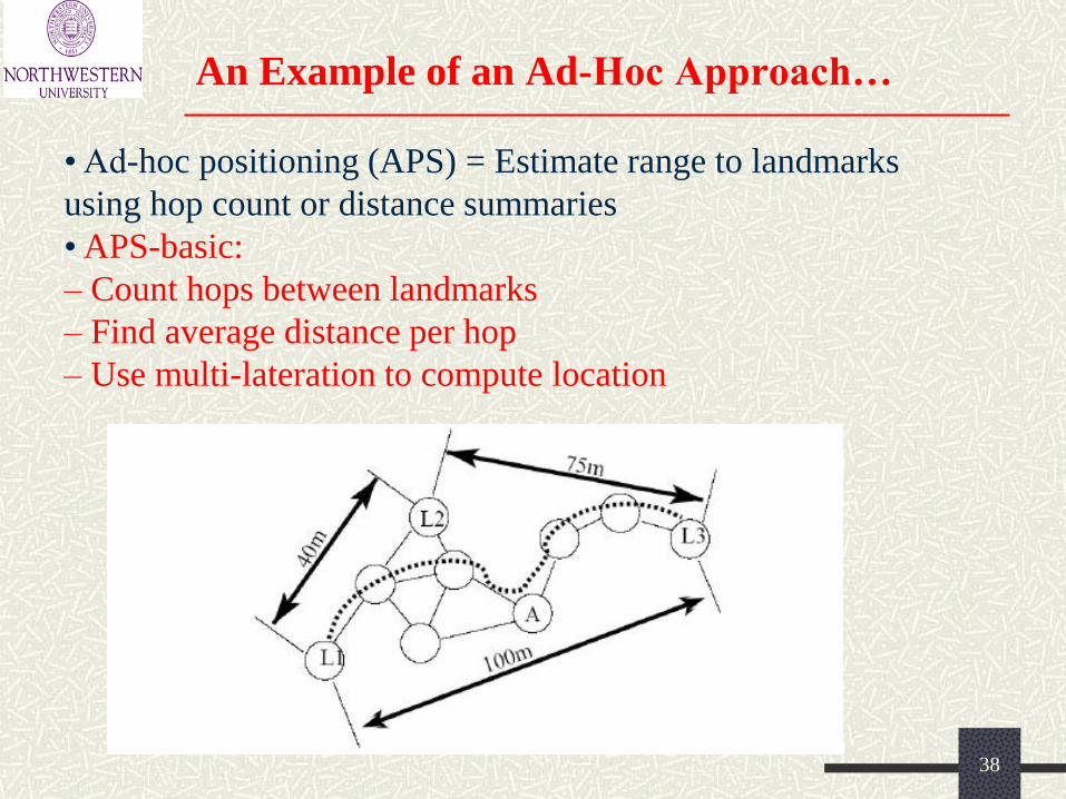
An Example of an Ad-Hoc Approach…

• Ad-hoc positioning (APS) = Estimate range to landmarks

using hop count or distance summaries

• APS-basic:

– Count hops between landmarks

– Find average distance per hop

– Use multi-lateration to compute location

39

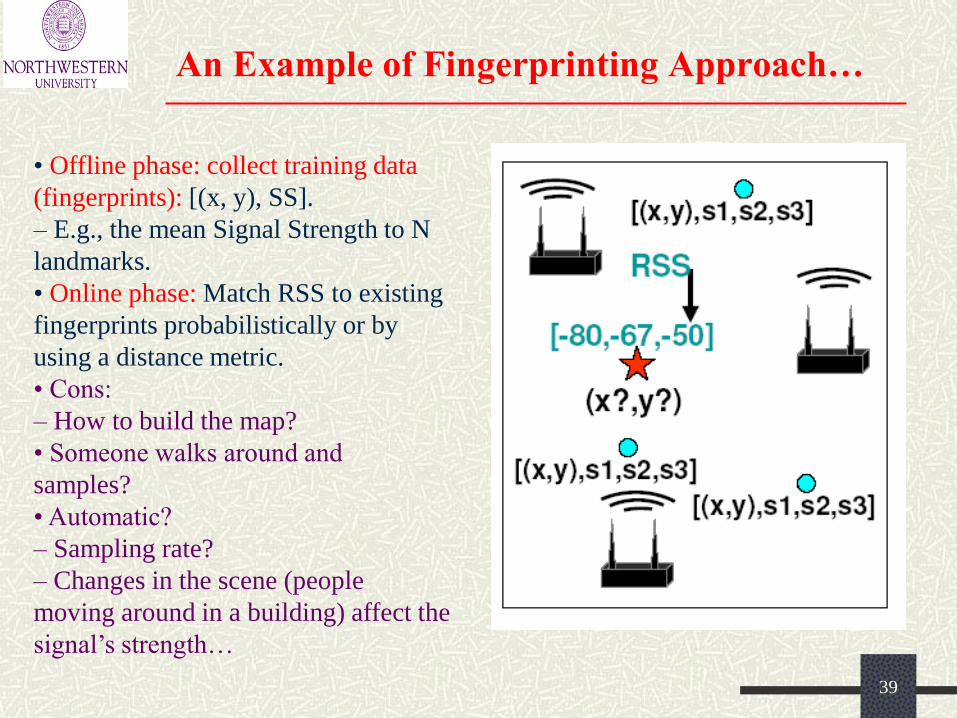
An Example of Fingerprinting Approach…

• Offline phase: collect training data

(fingerprints): [(x, y), SS].

– E.g., the mean Signal Strength to N

landmarks.

• Online phase: Match RSS to existing

fingerprints probabilistically or by

using a distance metric.

• Cons:

– How to build the map?

• Someone walks around and

samples?

• Automatic?

– Sampling rate?

– Changes in the scene (people

moving around in a building) affect the

signal’s strength…

40

GPS Overview

History

U.S. Department of Defense wanted the military to

have a super precise form of worldwide positioning

After $12B, the result was the GPS system!

Approach

“Man-made stars" as reference points to

calculate positions accurate to a matter of

meters

With advanced forms of GPS you can make

measurements to better than a centimeter

It's like giving every square meter on the

planet a unique address!

41

GPS Overview

Constellation of 24 NAVSTAR satellites made by Rockwell

Altitude: 10,900 nautical miles

Weight: 1900 lbs (in orbit)

Size: 17 ft with solar panels extended

Orbital Period: 12 hours

Orbital Plane: 55 degrees to equitorial plane

Planned Lifespan: 7.5 years

Current Constellation: 24 Block II production satellites

Future Satellites: 21 Block IIrs developed by Martin Marietta

Ground Stations, aka “Control Segment”

Monitor the GPS satellites, checking both their operational health and their exact position in space

Five monitor stations

Hawaii, Ascension Island, Diego Garcia, Kwajalein,

and Colorado Springs.

42

GPS – Basic Operation Principles

1. The basis of GPS is “trilateration" from satellites.

(popularly but wrongly called “triangulation”)

2. To “trilaterate," a GPS receiver measures distance

using the travel time of radio signals.

3. To measure travel time, GPS needs very accurate

timing which it achieves with some tricks.

4. Along with distance, you need to know exactly

where the satellites are in space. High orbits and

careful monitoring are the secret.

5. Finally you must correct for any delays the signal

experiences as it travels through the atmosphere.

43

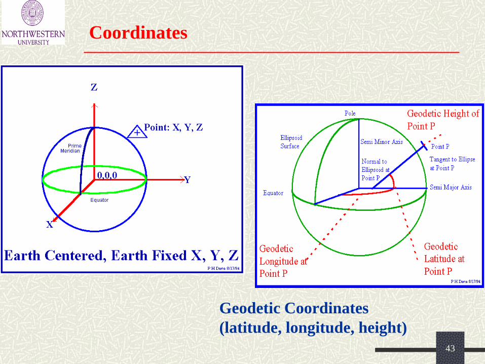
Coordinates

Geodetic Coordinates

(latitude, longitude, height)

44

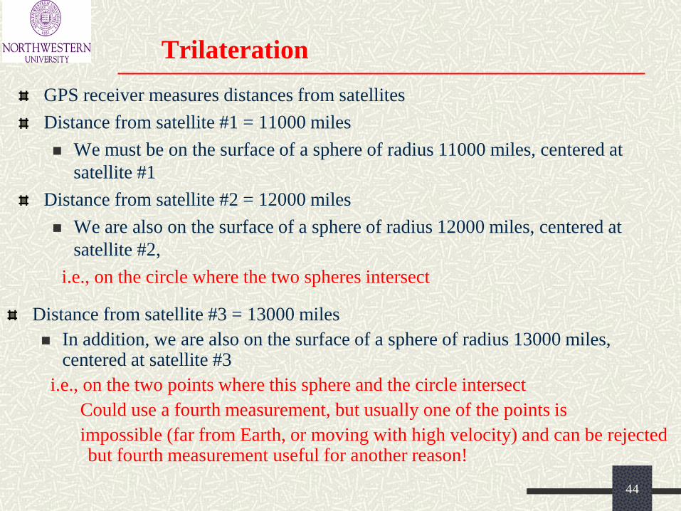
Trilateration

GPS receiver measures distances from satellites

Distance from satellite #1 = 11000 miles

We must be on the surface of a sphere of radius 11000 miles, centered at

satellite #1

Distance from satellite #2 = 12000 miles

We are also on the surface of a sphere of radius 12000 miles, centered at

satellite #2,

i.e., on the circle where the two spheres intersect

Distance from satellite #3 = 13000 miles

In addition, we are also on the surface of a sphere of radius 13000 miles, centered at satellite #3

i.e., on the two points where this sphere and the circle intersect

Could use a fourth measurement, but usually one of the points is

impossible (far from Earth, or moving with high velocity) and can be rejected but fourth measurement useful for another reason!

45

Measuring Distances from Satellites

By timing how long it takes for a signal sent from the satellite to arrive at the

receiver

We already know the speed of light

Timing problem is tricky

Smallest distance - 0.06 seconds

Need some really precise clocks

Thousandth of a second error 200 miles of error

On satellite side, atomic clocks provide almost perfectly

stable and accurate timing

What about on the receiver side?

Atomic clocks too expensive!

OK, but even assuming precise clocks, how do we measure travel

times?

46

Measuring Travel Times from Satellites

Each satellite transmits a unique pseudo-random code, a copy of which is created in real time in the user-set receiver by the internal electronics

The receiver then gradually time-shifts its internal code until it corresponds to the received code--an event called lock-on.

Once locked on to a satellite, the receiver can

determine the exact timing of the received signal in reference to its own internal clock

If receiver clock was perfectly synchronized, three satellites would be enough

In real GPS receivers, the internal clock is not quite accurate enough

The clock bias error can be determined by locking on to four satellites, and solving for X, Y, and Z coordinates, and the clock bias error

47

Extra Satellite Measurement to Eliminate Clock

Errors

Three perfect measurements can locate a point in 3D

Four imperfect measurements can do the same thing

If there is error in receiver clock, the fourth measurement will not intersect with the first three

Receiver looks for a single correction factor

The correction factor can then be applied to all

measurements from then on.

From then on its clock is synced to universal time.

This correction process would have to be repeated

constantly to make sure the receiver's clocks stay

synched

=> At least four channels are required for four

simultaneous measurements

48

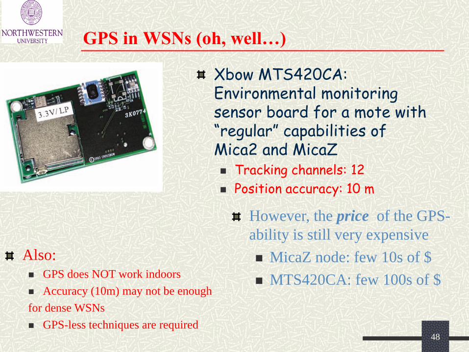
GPS in WSNs (oh, well…)

Xbow MTS420CA: Environmental monitoring sensor board for a mote with “regular” capabilities of Mica2 and MicaZ Tracking channels: 12

Position accuracy: 10 m

However, the price of the GPS-

ability is still very expensive

MicaZ node: few 10s of $

MTS420CA: few 100s of $

Also:

GPS does NOT work indoors

Accuracy (10m) may not be enough

for dense WSNs

GPS-less techniques are required

49

GPS-less Techniques

Use DISTANCE or ANGLE measurements from a set of fixed reference points and apply

MULTI-LATERATION or TRIANGULATION techniques.

Basic approaches:

a. Received Signal Strength (RSS)

b. Time of Arrival (TOA)

c. Time Difference of Arrival (TDOA)

d. Angle of Arrival (AOA)

50

Received Signal Strength (RSS)

IDEA:

Use some readily-available info to estimate the distance between a transmitter and a receiver:

a. The Power of the Received Signal

b. Knowledge of Transmitter Power

c. Path Loss Model

Crux:

Each measurement gives a circle on which the sensor must lie…

Note: RSS method may be unreliable/inaccurate due to:

a. Multi-path effects

b. Shadowing, scattering, and other impairments

c. Non line-of-sight conditions

51

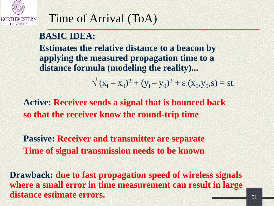
Time of Arrival (ToA)

BASIC IDEA:

Estimates the relative distance to a beacon by applying the measured propagation time to a distance formula (modeling the reality)...

√ (xi – x0)2 + (yi – y0)

2 + i(x0,y0,s) = sti

Active: Receiver sends a signal that is bounced back

so that the receiver know the round-trip time

Passive: Receiver and transmitter are separate

Time of signal transmission needs to be known

Drawback: due to fast propagation speed of wireless signals where a small error in time measurement can result in large distance estimate errors.

52

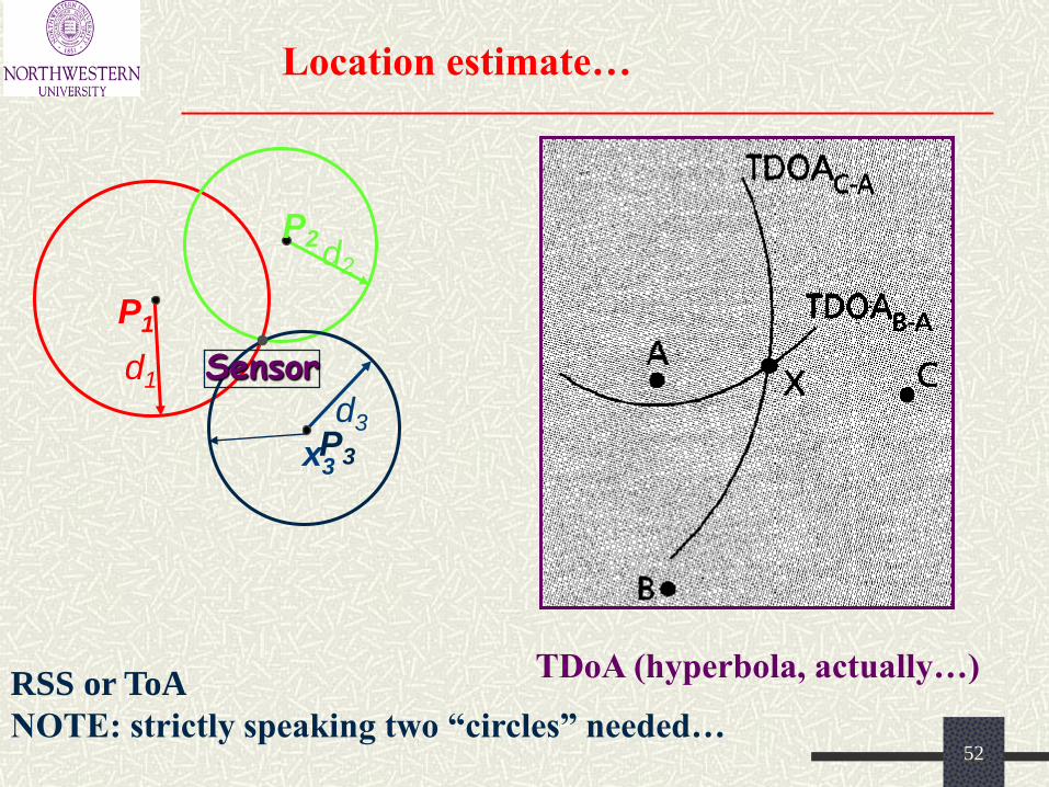
Location estimate…

P1

P2

x3

d1

d3

d2

Sensor

P3

RSS or ToA

NOTE: strictly speaking two “circles” needed…

TDoA (hyperbola, actually…)

53

Time or Time Difference of Arrival

(ToA/TDoA)

Time synchronized beacons and nodes that send

periodic announcement also enable the node to

calculate an estimate of its distance from other nodes.

This can be achieved by calculating the time difference

of the expected and actual arrival of a signal, taking

into account possible interference and propagation

delay.

54

Angle of Arrival (AoA)

Special antenna configurations are used to estimate the angle

of arrival of the received signal from a beacon node.

Angle of arrival method may also be unreliable and inaccurate due to:

a. Multi-path effects,

b. Shadowing, scattering, and other impairments,

c. Non line of sight conditions.

55

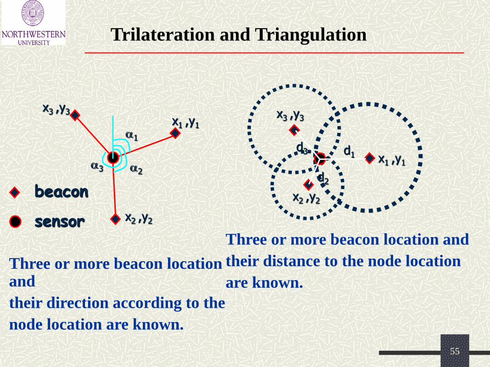
Trilateration and Triangulation

1

2 3

x1 ,y1

x2 ,y2

x3 ,y3

beacon

sensor

Three or more beacon location and

their direction according to the

node location are known.

Three or more beacon location and

their distance to the node location

are known.

d1 x1 ,y1

x2 ,y2

x3 ,y3

d2

d3

56

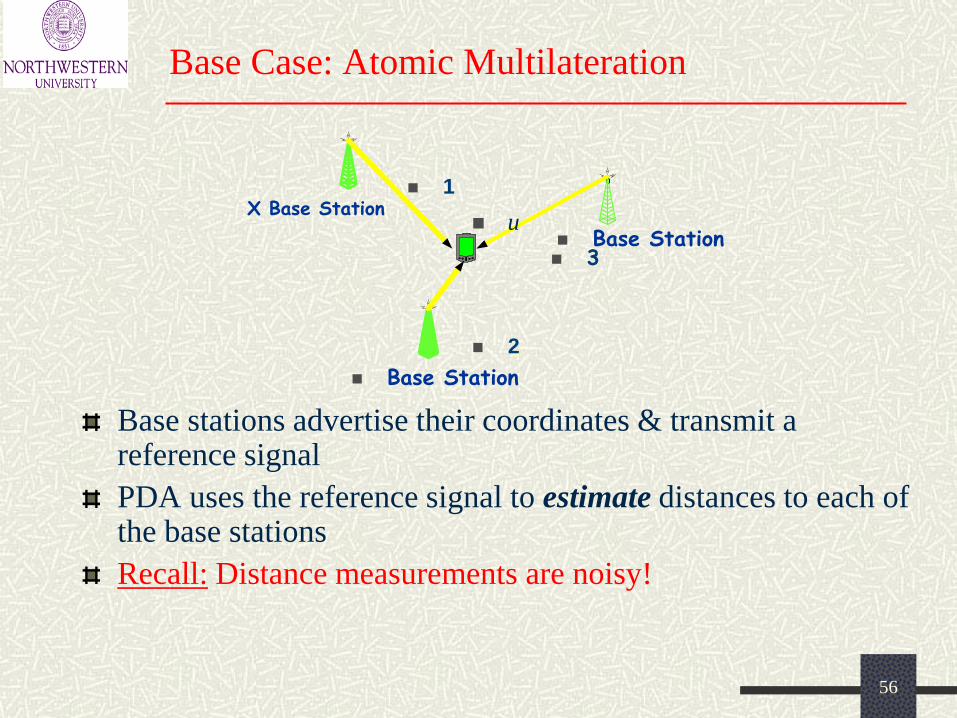
Base Case: Atomic Multilateration

Base stations advertise their coordinates & transmit a reference signal

PDA uses the reference signal to estimate distances to each of the base stations

Recall: Distance measurements are noisy!

X Base Station 1

Base Station 3

Base Station

2

u

57

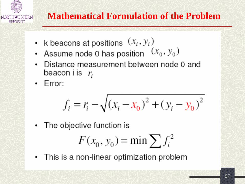
Mathematical Formulation of the Problem

58

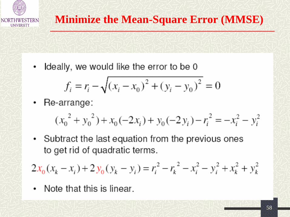
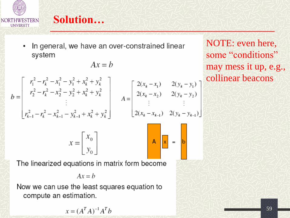
Minimize the Mean-Square Error (MMSE)

59

Solution…

NOTE: even here,

some “conditions”

may mess it up, e.g.,

collinear beacons

60

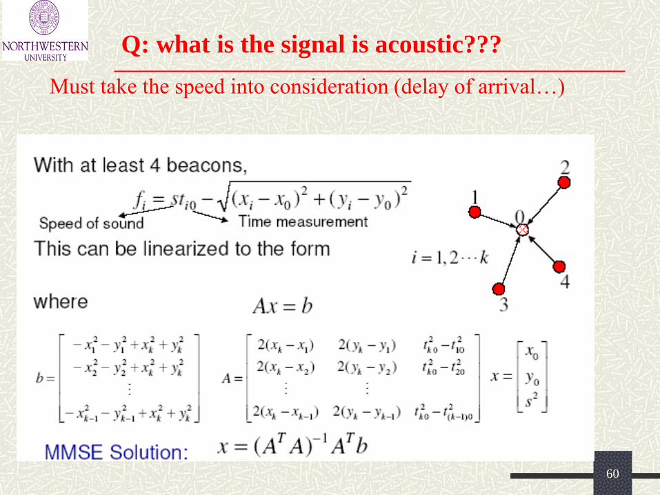
Q: what is the signal is acoustic???

Must take the speed into consideration (delay of arrival…)

61

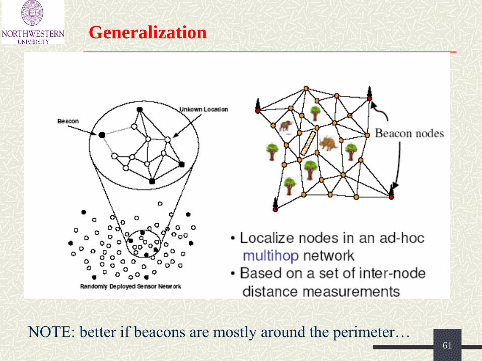
Generalization

NOTE: better if beacons are mostly around the perimeter…

62

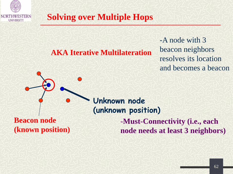
Solving over Multiple Hops

AKA Iterative Multilateration

Beacon node

(known position)

Unknown node (unknown position)

-A node with 3

beacon neighbors

resolves its location

and becomes a beacon

-Must-Connectivity (i.e., each

node needs at least 3 neighbors)

63

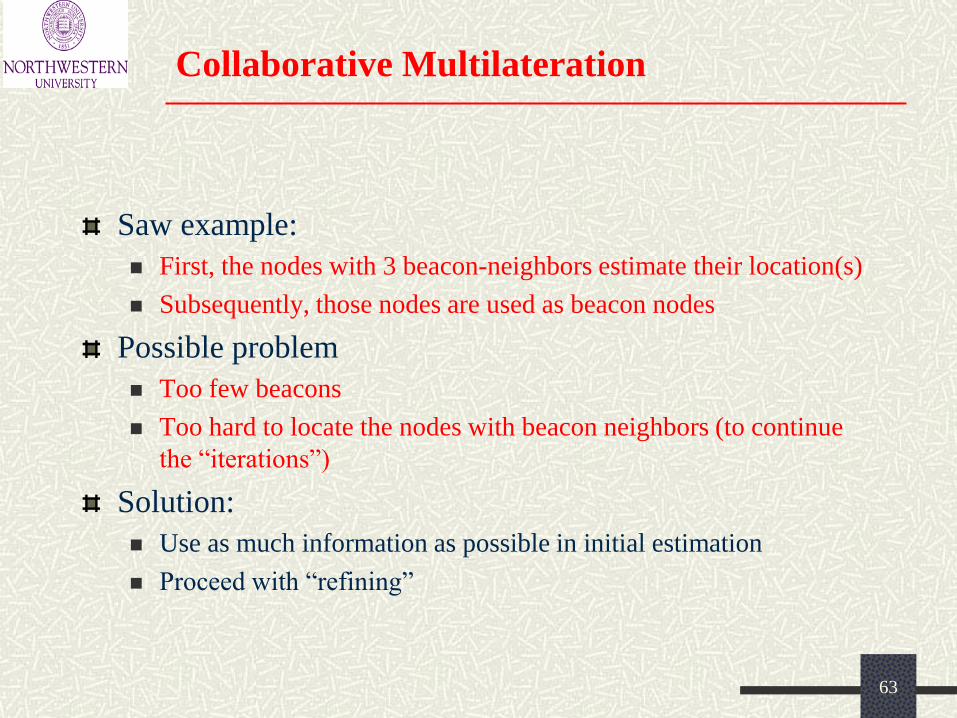
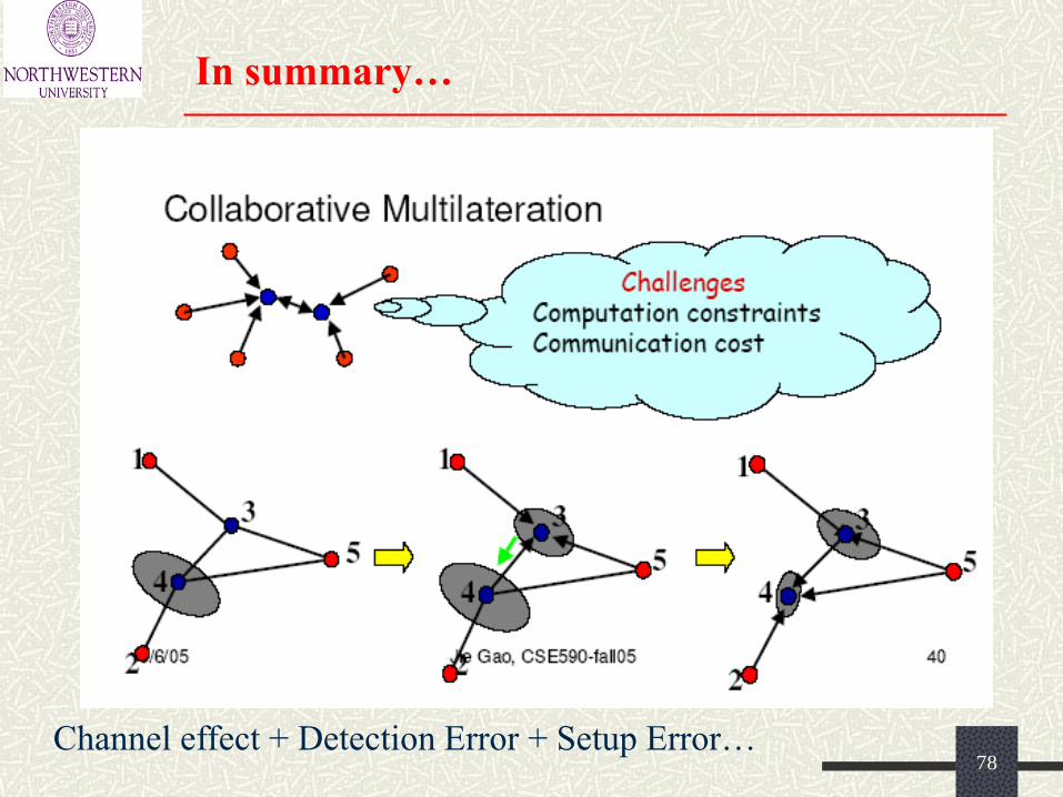
Collaborative Multilateration

Saw example:

First, the nodes with 3 beacon-neighbors estimate their location(s)

Subsequently, those nodes are used as beacon nodes

Possible problem

Too few beacons

Too hard to locate the nodes with beacon neighbors (to continue

the “iterations”)

Solution:

Use as much information as possible in initial estimation

Proceed with “refining”

64

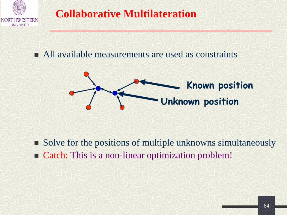
Collaborative Multilateration

All available measurements are used as constraints

Solve for the positions of multiple unknowns simultaneously

Catch: This is a non-linear optimization problem!

Known position

Unknown position

65

The n-hop Multilateration Problem

Assumptions

Few of the nodes (if at all) are equipped with GPS (GPS-less)

A fraction of the nodes, called the beacons, are aware of their

locations, others are referred as the unknowns

All the nodes within radio range of each other can measure the

distance between each other

66

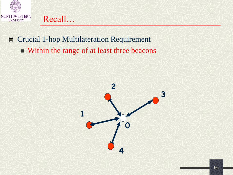
Recall…

Crucial 1-hop Multilateration Requirement

Within the range of at least three beacons

4

0

1

2 3

67

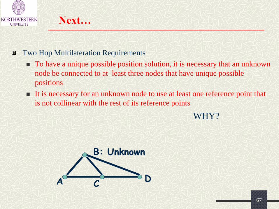
Next…

Two Hop Multilateration Requirements

To have a unique possible position solution, it is necessary that an unknown

node be connected to at least three nodes that have unique possible

positions

It is necessary for an unknown node to use at least one reference point that

is not collinear with the rest of its reference points

B: Unknown

A C D

WHY?

68

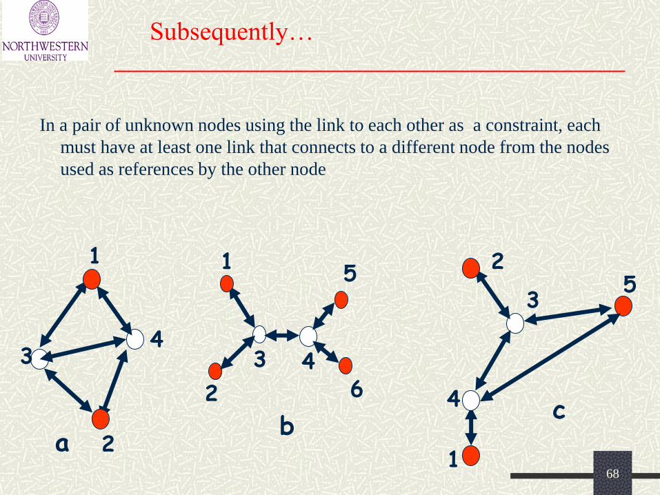
Subsequently…

In a pair of unknown nodes using the link to each other as a constraint, each

must have at least one link that connects to a different node from the nodes

used as references by the other node

a

4

1

2

3

b

4 3

1

2

5

6 c 4

5

1

2

3

69

First Step in Multilatiration

N-hop multilateration requirement

Have three neighbors that have unique positions?

Ask its unknown neighbor to determine its position

Assume the caller has tentatively unique solution

Meet the constraints

Do it recursively

70

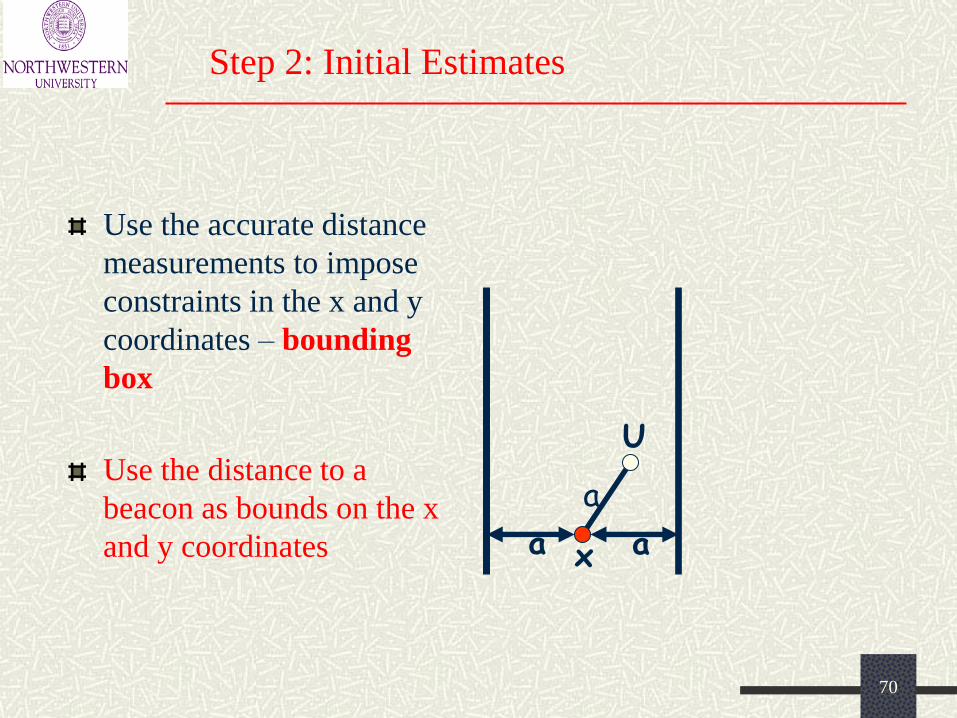
Step 2: Initial Estimates

Use the accurate distance

measurements to impose

constraints in the x and y

coordinates – bounding

box

Use the distance to a

beacon as bounds on the x

and y coordinates

a

a a x

U

71

Step 2: Multiple Initial Estimates

Use the accurate distance measurements to impose constraints in the x and y coordinates – bounding box

Do the same for beacons that are multiple hops away Node Y in the Figure…

Select the most constraining bounds a

b

c

b+c b+c

X

Y

U

U is between [Y-(b+c)] and [X+a]

72

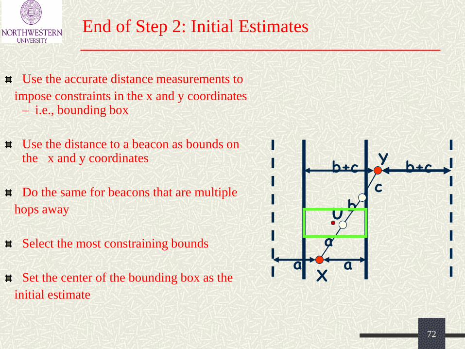
End of Step 2: Initial Estimates

Use the accurate distance measurements to

impose constraints in the x and y coordinates – i.e., bounding box

Use the distance to a beacon as bounds on the x and y coordinates

Do the same for beacons that are multiple

hops away

Select the most constraining bounds

Set the center of the bounding box as the

initial estimate

a

a a

b c

b+c b+c

X

Y

U

73

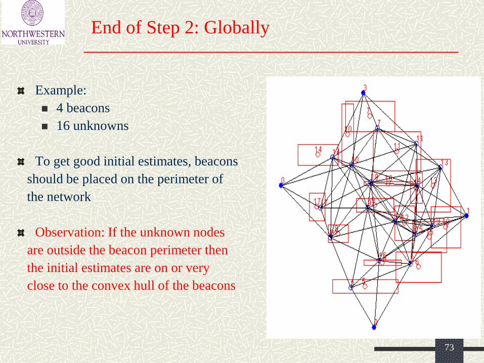
End of Step 2: Globally

Example:

4 beacons

16 unknowns

To get good initial estimates, beacons

should be placed on the perimeter of

the network

Observation: If the unknown nodes

are outside the beacon perimeter then

the initial estimates are on or very

close to the convex hull of the beacons

74

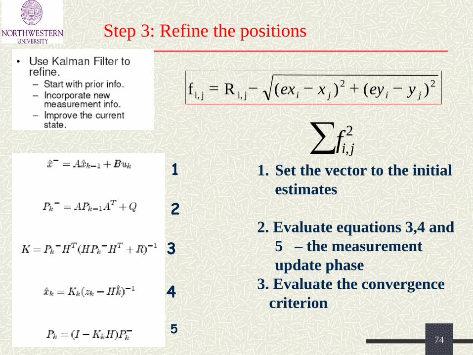
Step 3: Refine the positions

1

2

3

4

5

1. Set the vector to the initial

estimates

2. Evaluate equations 3,4 and

5 – the measurement

update phase

3. Evaluate the convergence

criterion

2

, j i f

2 2

j i, j i, ) ( ) ( R f j i j i y ey x ex

75

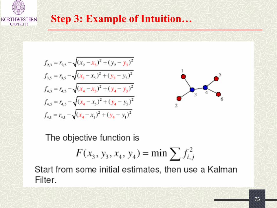
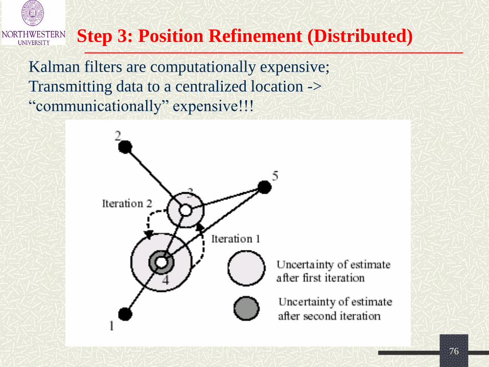
Step 3: Example of Intuition…

76

Step 3: Position Refinement (Distributed)

Kalman filters are computationally expensive;

Transmitting data to a centralized location ->

“communicationally” expensive!!!

77

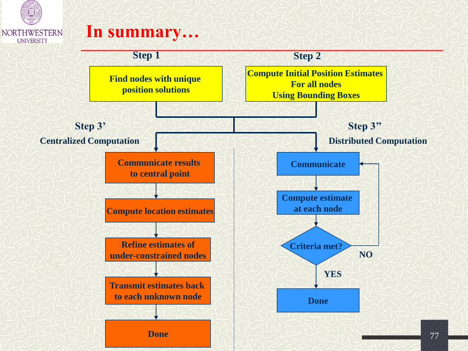
In summary…

Find nodes with unique

position solutions

Compute Initial Position Estimates

For all nodes

Using Bounding Boxes

Compute location estimates

Compute estimate

at each node

Communicate

Criteria met?

YES

NO

Communicate results

to central point

Transmit estimates back

to each unknown node

Refine estimates of

under-constrained nodes

Done

Done

Centralized Computation Distributed Computation

Step 1 Step 2

Step 3’ Step 3’’

78

In summary…

Channel effect + Detection Error + Setup Error…

79

In Summary…

Localization:

Still many open problems

Design decisions based on availability of technology, and constraints of the

operating environment

Can we have powerful computation?

What is the availability of infrastructure support?

What type of obstructions are in the environment?

How fast, accurate, reliable should the localization process be?

(very domain-specific…)

80

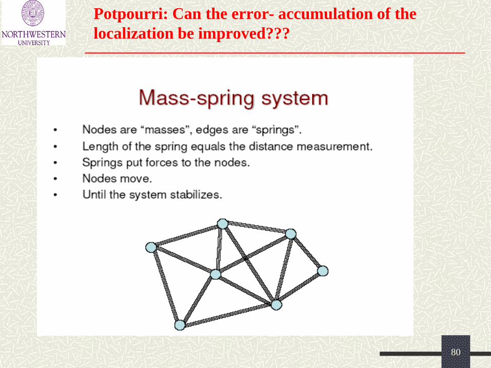
Potpourri: Can the error- accumulation of the

localization be improved???

81

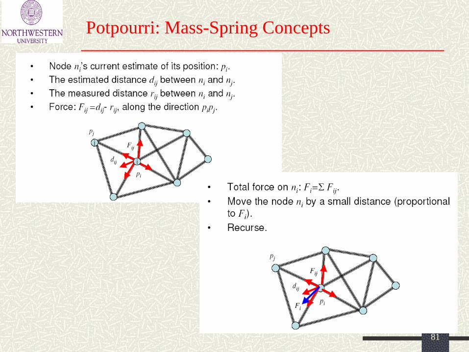
Potpourri: Mass-Spring Concepts

82

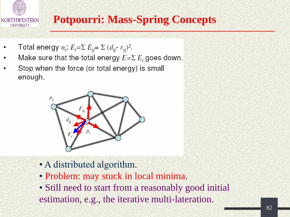
Potpourri: Mass-Spring Concepts

• A distributed algorithm.

• Problem: may stuck in local minima.

• Still need to start from a reasonably good initial

estimation, e.g., the iterative multi-lateration.

83

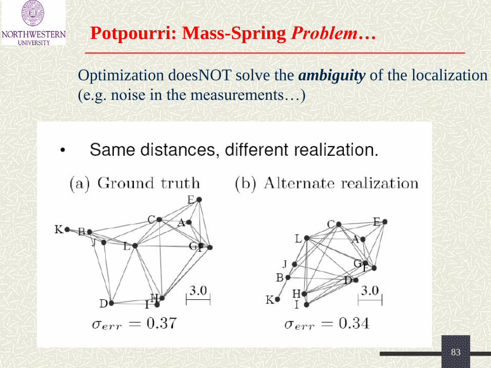
Potpourri: Mass-Spring Problem…

Optimization doesNOT solve the ambiguity of the localization

(e.g. noise in the measurements…)

84

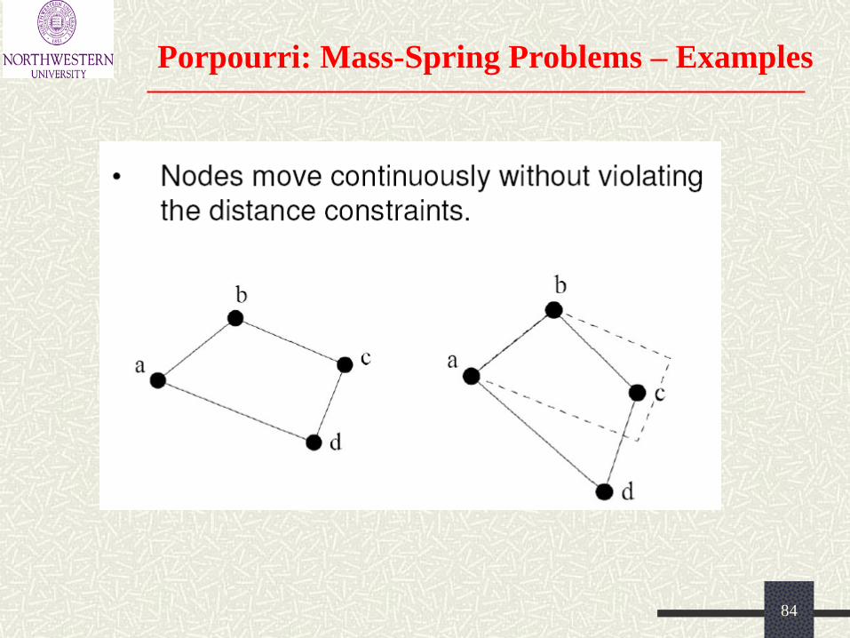
Porpourri: Mass-Spring Problems – Examples

85

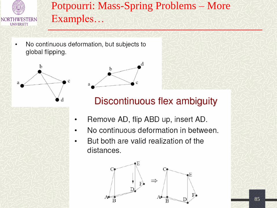
Potpourri: Mass-Spring Problems – More

Examples…

86

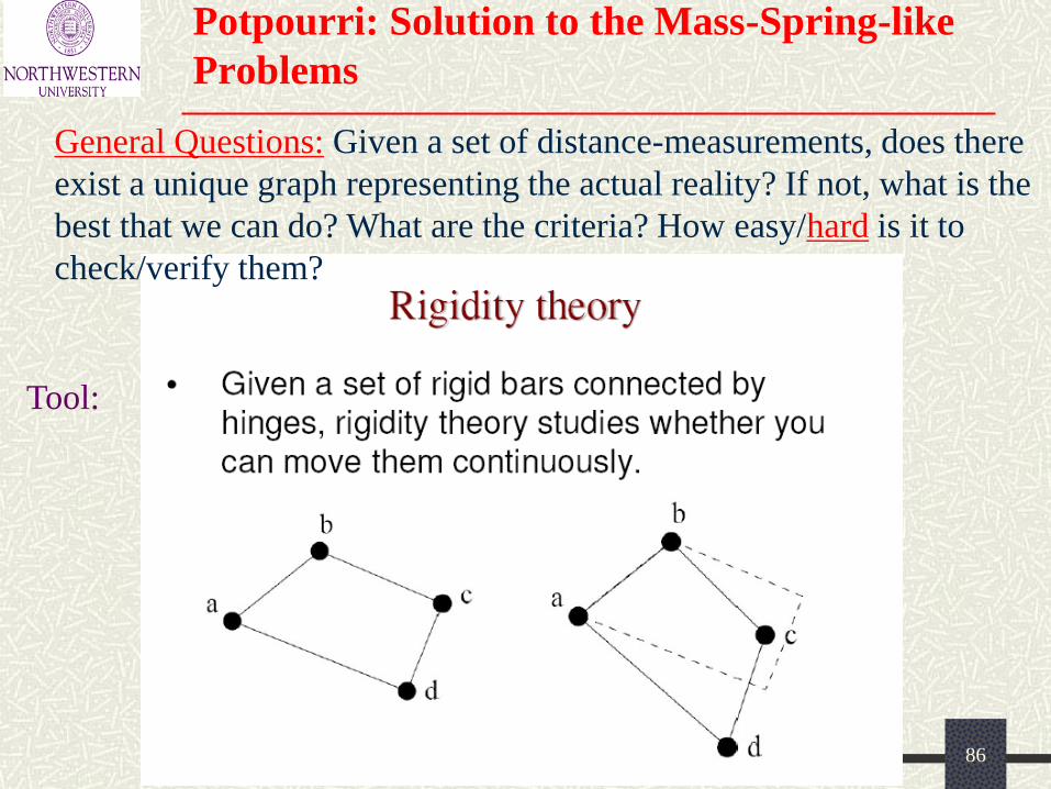
Potpourri: Solution to the Mass-Spring-like

Problems

General Questions: Given a set of distance-measurements, does there

exist a unique graph representing the actual reality? If not, what is the

best that we can do? What are the criteria? How easy/hard is it to

check/verify them?

Tool:

87

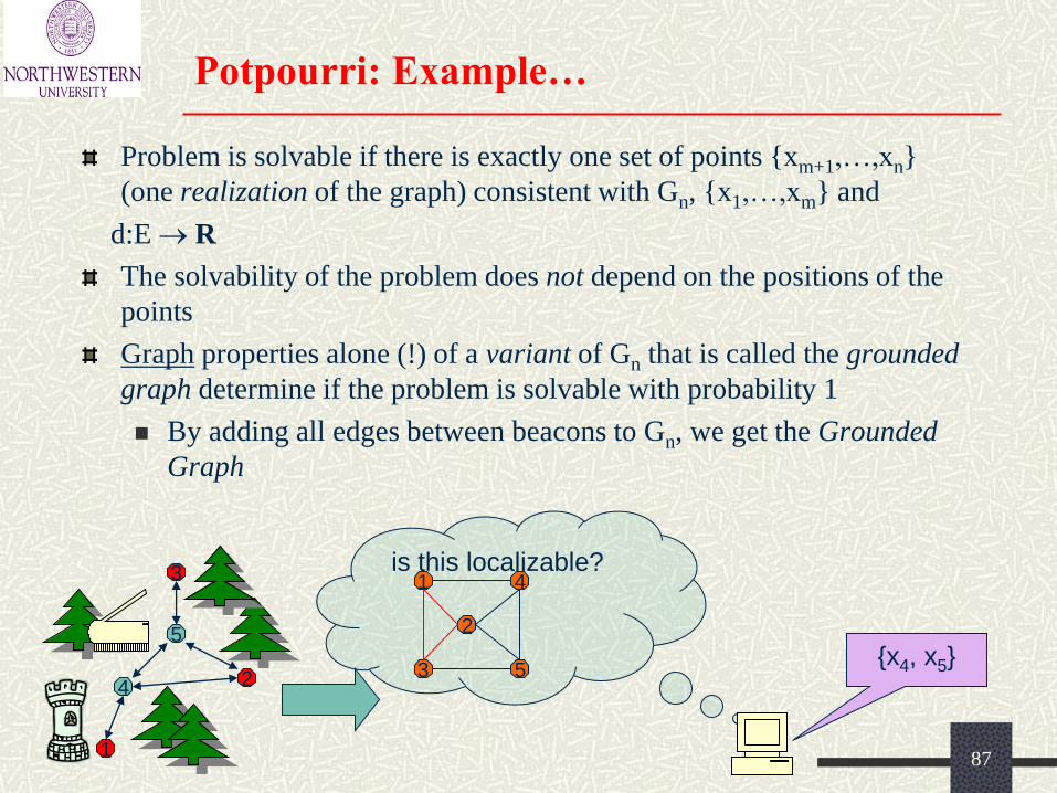
Potpourri: Example…

Problem is solvable if there is exactly one set of points {xm+1,…,xn}

(one realization of the graph) consistent with Gn, {x1,…,xm} and

d:E R

The solvability of the problem does not depend on the positions of the

points

Graph properties alone (!) of a variant of Gn that is called the grounded

graph determine if the problem is solvable with probability 1

By adding all edges between beacons to Gn, we get the Grounded

Graph

is this localizable?

5

4

1

2

3 1

2

3

4

5 {x4, x5}

88

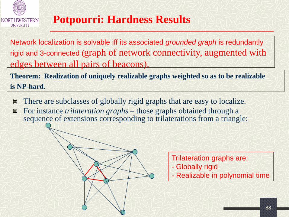
Potpourri: Hardness Results

There are subclasses of globally rigid graphs that are easy to localize.

For instance trilateration graphs – those graphs obtained through a sequence of extensions corresponding to trilaterations from a triangle:

Theorem: Realization of uniquely realizable graphs weighted so as to be realizable

is NP-hard.

Trilateration graphs are:

- Globally rigid

- Realizable in polynomial time

Network localization is solvable iff its associated grounded graph is redundantly

rigid and 3-connected (graph of network connectivity, augmented with

edges between all pairs of beacons).

89

Readings…

A. Savvides, L. Girod, M. Srivastava, and D. Estrin, "Localization in

Sensor Networks," Book Chapter in: Wireless Sensor Networks,

Edited by Znati, Radhavendra and Sivalingam, Kluwer Academic

Publishers, 2004.

B. Sundararaman, U. Buy, A. D. Kshemkalyani, "Clock

synchronization for wireless sensor networks: a survey" Ad Hoc

Networks 3 (2005) 281–323, 2005

Additional/Recommended:

Lecture notes on Rigidity Theory by Prof. Jie Gao (Dept. of Computer Science,

SUNY at Stony Brook)

“Mobile-Assisted Localization in Wireless Sensor Networks”, N.B. Priyantha, H.

Balakrishnan, E. Demaine, S. Teller, IEEE INFOCOM 2005.