Embed Size (px)
Citation preview
EE6882 Statistical Methods for Video Indexing and Analysis
Lecture 2 (09/17/07)
Fall 2007
Lexing Xie
Lecture Outline
� The content-based multimedia retrieval problem
� System components
� Describing multimedia content
� Image features
� Color, Texture, others
� Audio and text features
� Video representation and description � next week by Eric
� Distance metrics
� Evaluation of retrieval systems
� Guidelines for paper reading and presentation
� You questions: color quantization, perception vs. indexing
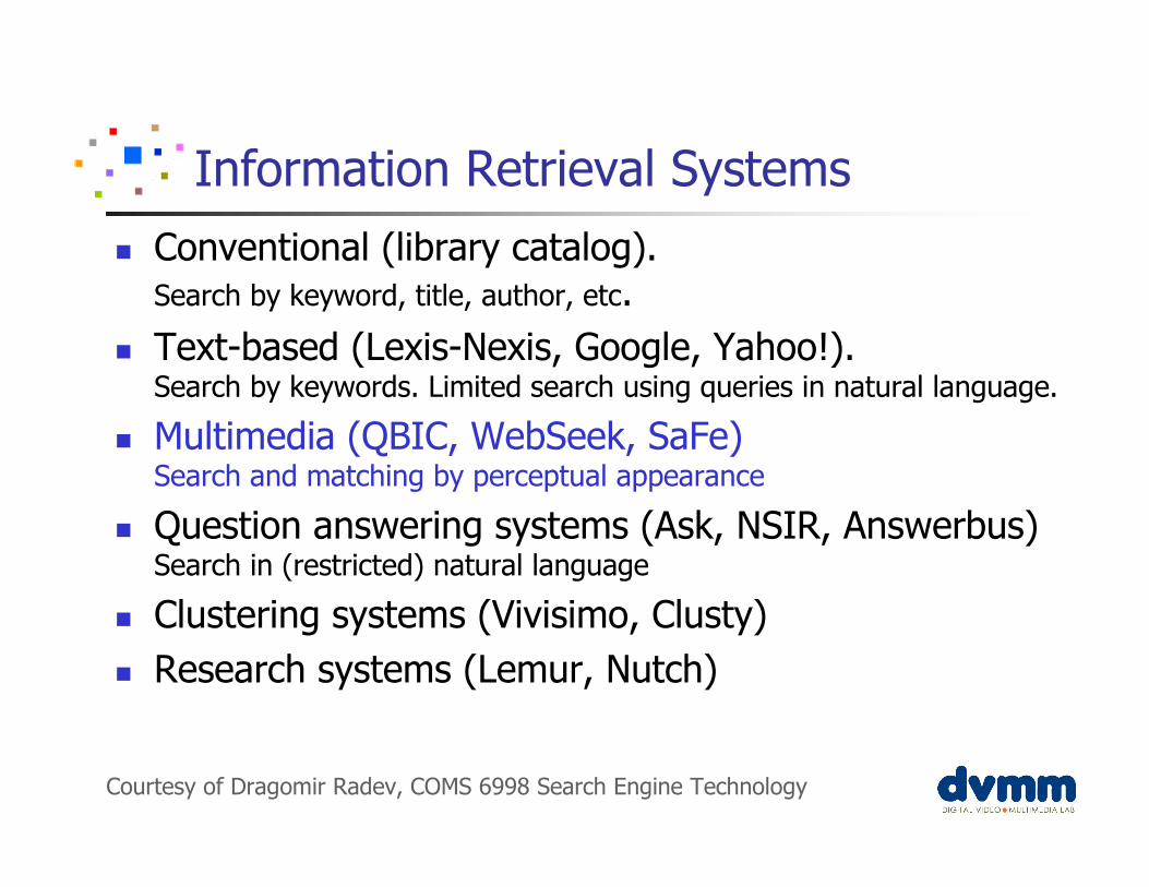
Information Retrieval Systems
� Conventional (library catalog). Search by keyword, title, author, etc.
� Text-based (Lexis-Nexis, Google, Yahoo!).Search by keywords. Limited search using queries in natural language.
� Multimedia (QBIC, WebSeek, SaFe)Search and matching by perceptual appearance
� Question answering systems (Ask, NSIR, Answerbus)Search in (restricted) natural language
� Clustering systems (Vivisimo, Clusty)
� Research systems (Lemur, Nutch)
Courtesy of Dragomir Radev, COMS 6998 Search Engine Technology
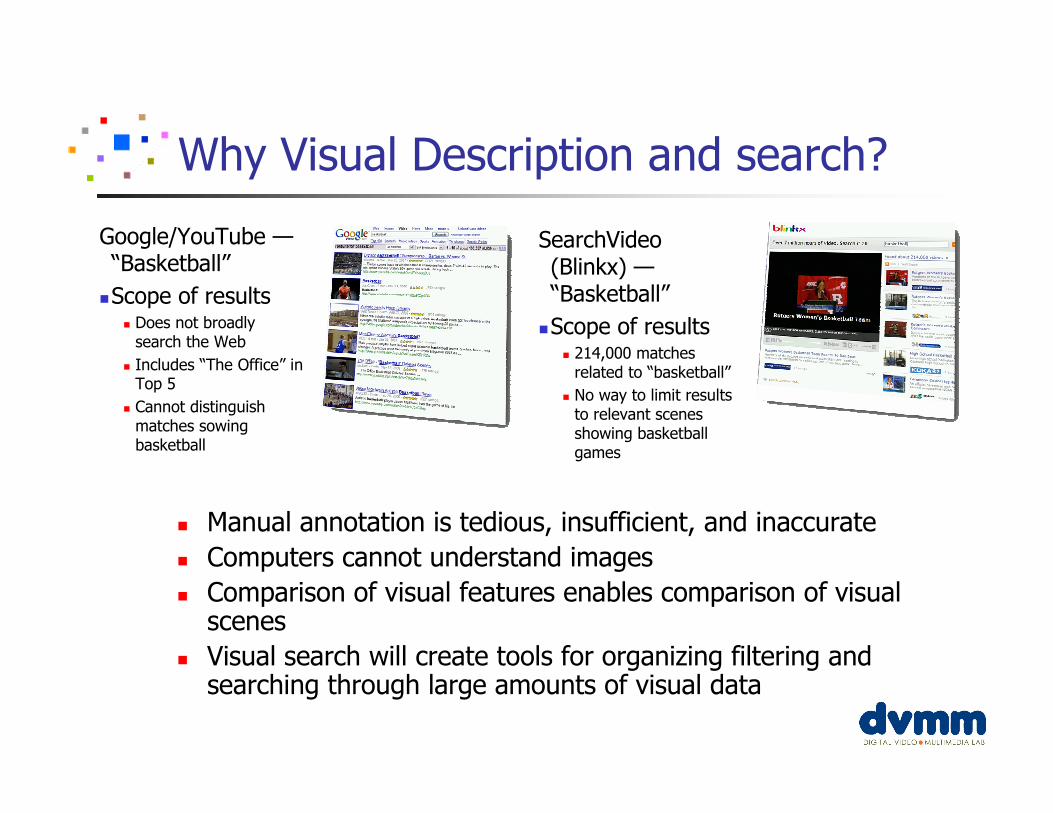
Why Visual Description and search?
Google/YouTube —“Basketball”
�Scope of results� Does not broadly search the Web
� Includes “The Office” in Top 5
� Cannot distinguish matches sowing basketball
SearchVideo (Blinkx) —“Basketball”
�Scope of results� 214,000 matches related to “basketball”
� No way to limit results to relevant scenes showing basketball games
� Manual annotation is tedious, insufficient, and inaccurate
� Computers cannot understand images
� Comparison of visual features enables comparison of visual scenes
� Visual search will create tools for organizing filtering and searching through large amounts of visual data
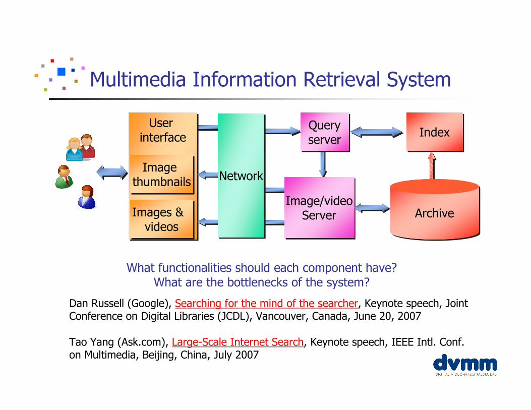
Multimedia Information Retrieval System
User interface
User interface
Image thumbnails
Image thumbnails
Images & videos
Images & videos
NetworkNetwork
Queryserver
Queryserver
Image/videoServer
Image/videoServer
IndexIndex
ArchiveArchive
Dan Russell (Google), Searching for the mind of the searcher, Keynote speech, Joint Conference on Digital Libraries (JCDL), Vancouver, Canada, June 20, 2007
Tao Yang (Ask.com), Large-Scale Internet Search, Keynote speech, IEEE Intl. Conf. on Multimedia, Beijing, China, July 2007
What functionalities should each component have?What are the bottlenecks of the system?
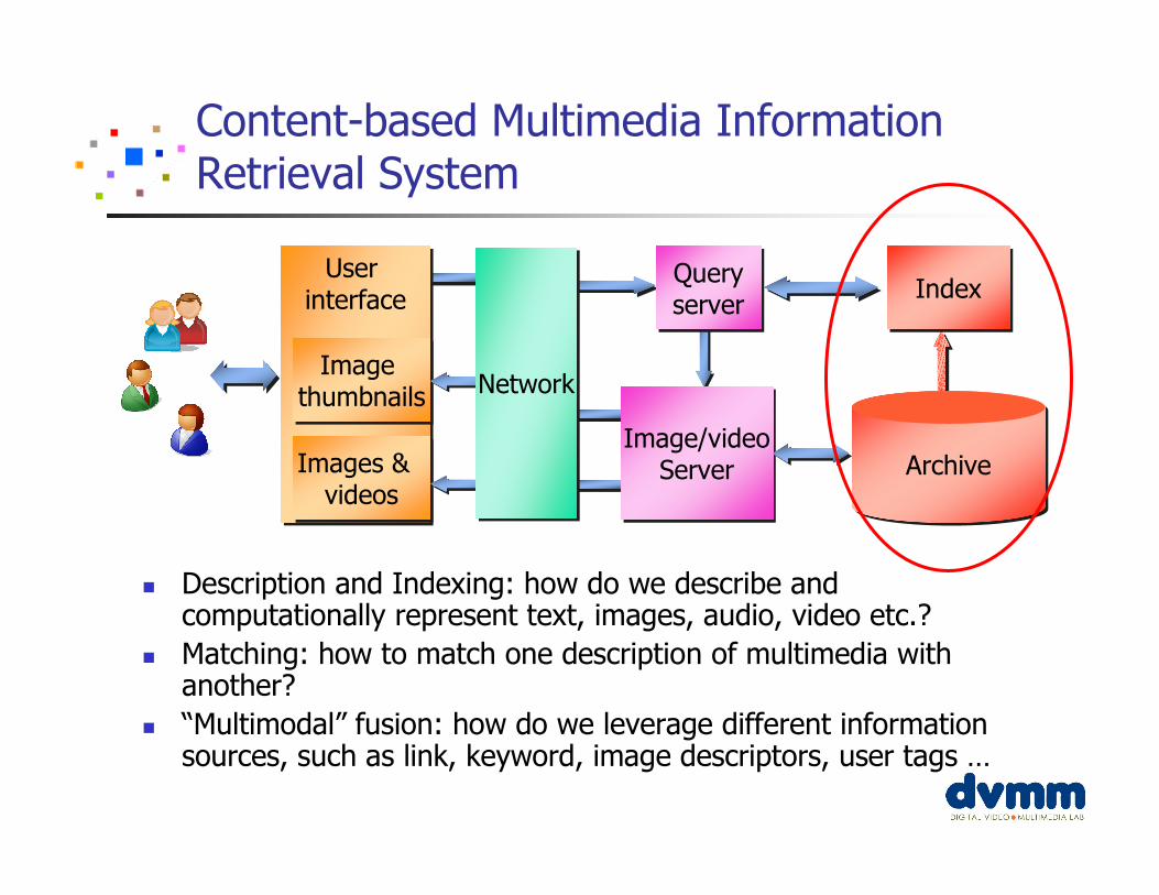
Content-based Multimedia Information Retrieval System
User interface
User interface
Image thumbnails
Image thumbnails
Images & videos
Images & videos
NetworkNetwork
Queryserver
Queryserver
Image/videoServer
Image/videoServer
IndexIndex
ArchiveArchive
� Description and Indexing: how do we describe and computationally represent text, images, audio, video etc.?
� Matching: how to match one description of multimedia with another?
� “Multimodal” fusion: how do we leverage different information sources, such as link, keyword, image descriptors, user tags …
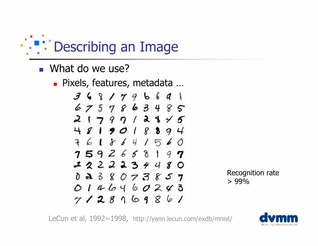
Describing an Image
� What do we use?
� Pixels, features, metadata …
LeCun et al, 1992~1998, http://yann.lecun.com/exdb/mnist/
Recognition rate > 99%
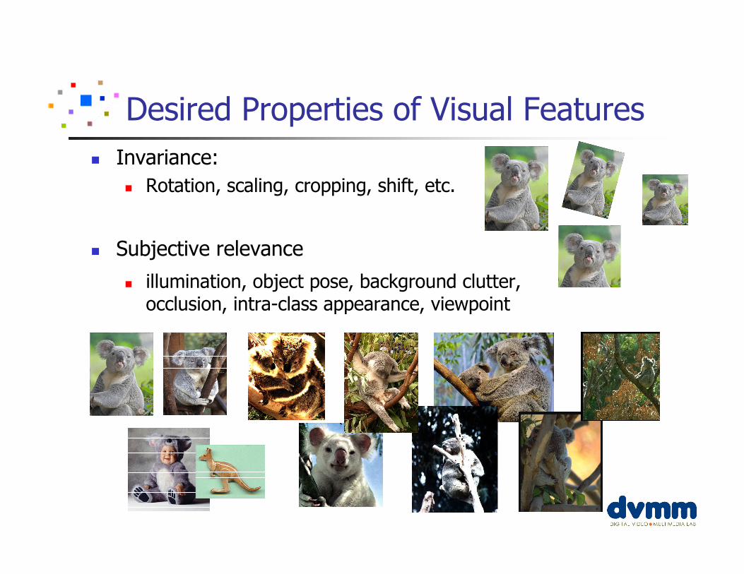
Desired Properties of Visual Features
� Invariance:
� Rotation, scaling, cropping, shift, etc.
� Subjective relevance
� illumination, object pose, background clutter, occlusion, intra-class appearance, viewpoint
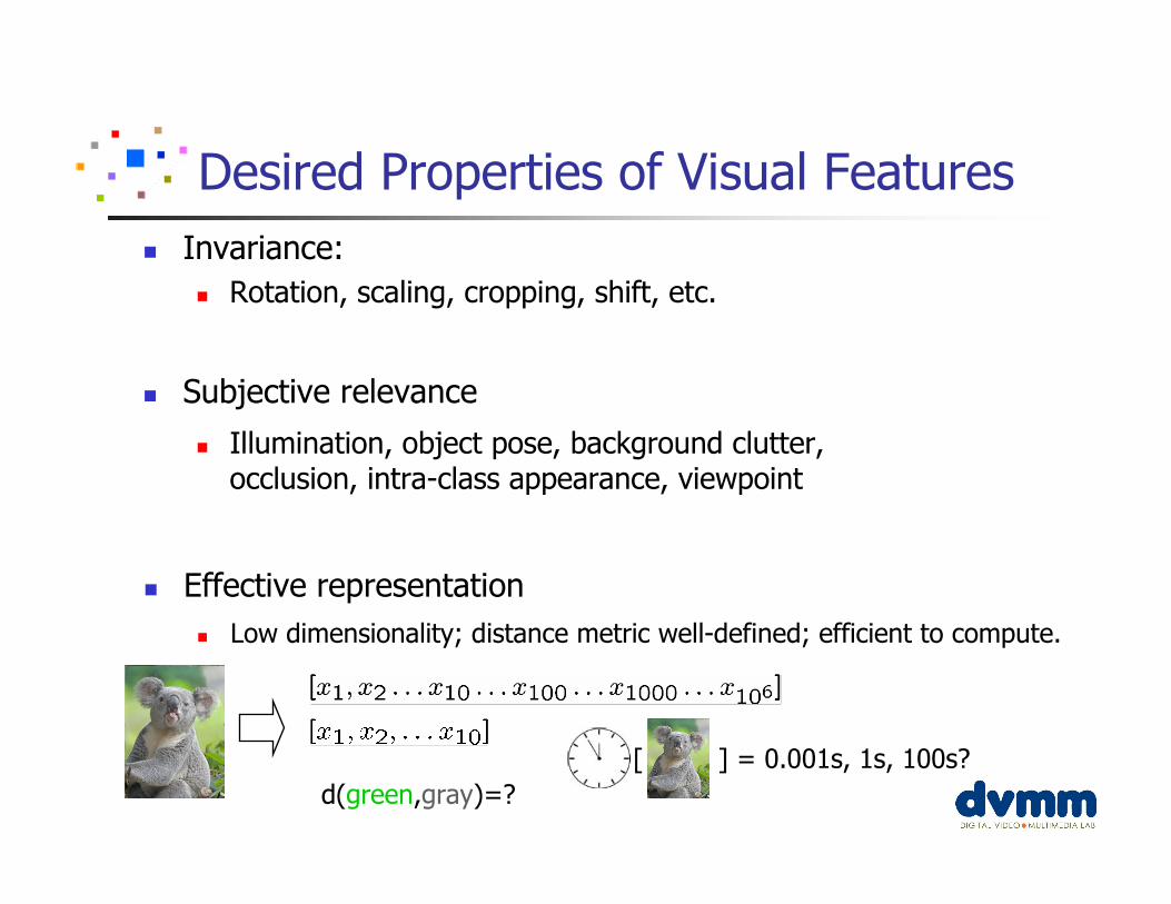
Desired Properties of Visual Features
� Effective representation
� Low dimensionality; distance metric well-defined; efficient to compute.
� Invariance:
� Rotation, scaling, cropping, shift, etc.
� Subjective relevance
� Illumination, object pose, background clutter, occlusion, intra-class appearance, viewpoint
d(green,gray)=?
[ ] = 0.001s, 1s, 100s?
Describing an Image
� What visual features?
� What is available in the data?
� What features does the human visual system (HVS) use?
� Color: beyond cats-and-dogs vision
� Texture: visual patterns, surface properties, cues for depth
� Shape: boundaries and measurement of real world objects and edges
� Motion: camera motion, object motion, depth from motion
General Approach for Visual Indexing
� Fundamental approach is from pattern recognition work
� Group pixels, process the group and generate a feature vector
� Summarize, if necessary, features over an entire image or unit of comparison (image patch, region, blob)
� Discrimination via (transform and ) feature vector distance
� Multidimensional indexing of the feature vectors
� This lecture: Do this for color and texture
� Build a content-based image retrieval system
Lecture Outline� The content-based multimedia retrieval problem
� System components
� Describing multimedia content
� Image features� Color, Texture, others
� Audio and text features
� Video representation and description
� Distance metric
� Evaluation of retrieval systems
� Guidelines for paper reading and presentation
� You questions: color quantization, perception vs. indexing
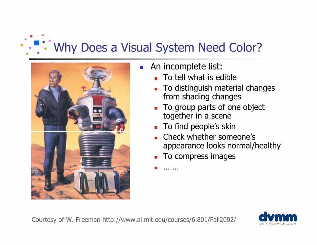
Why Does a Visual System Need Color?
Courtesy of W. Freeman http://www.ai.mit.edu/courses/6.801/Fall2002/
� An incomplete list:
� To tell what is edible
� To distinguish material changes from shading changes
� To group parts of one object together in a scene
� To find people’s skin
� Check whether someone’s appearance looks normal/healthy
� To compress images
� … …
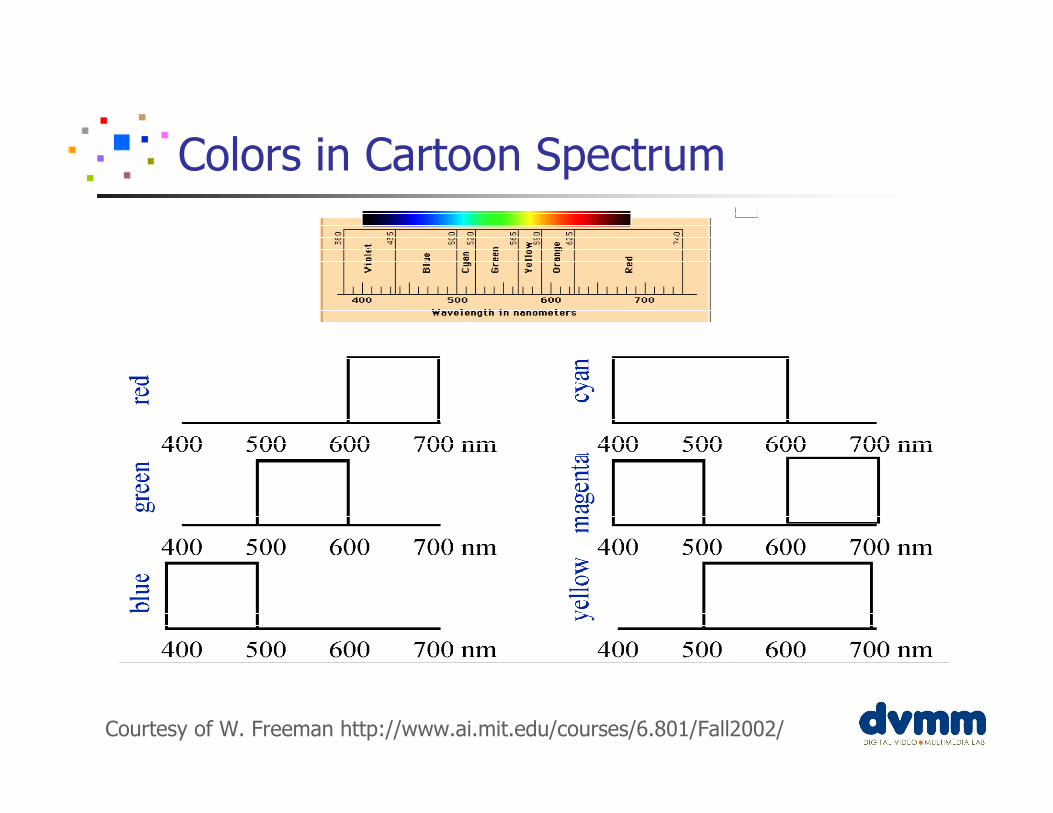
Colors in Cartoon Spectrum
Courtesy of W. Freeman http://www.ai.mit.edu/courses/6.801/Fall2002/
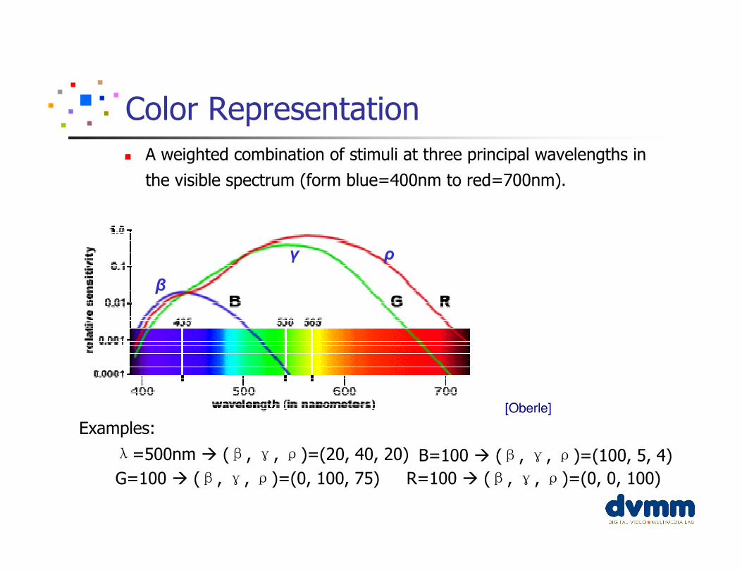
Color Representation
� A weighted combination of stimuli at three principal wavelengths in
the visible spectrum (form blue=400nm to red=700nm).
β
ργ
Examples:
λ=500nm � (β, γ, ρ)=(20, 40, 20) B=100 � (β, γ, ρ)=(100, 5, 4)
G=100 � (β, γ, ρ)=(0, 100, 75) R=100 � (β, γ, ρ)=(0, 0, 100)
[Oberle]
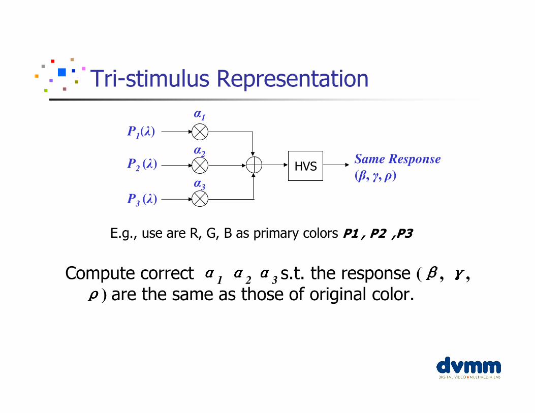
Tri-stimulus Representation
Compute correct αααα1 αααα2 αααα3 s.t. the response (ββββ, γγγγ,
ρρρρ) are the same as those of original color.
P1(λ)
P2 (λ)
P3 (λ)
α1
α2
α3
HVSSame Response
(β, γ, ρ)
E.g., use are R, G, B as primary colors P1 , P2 ,P3
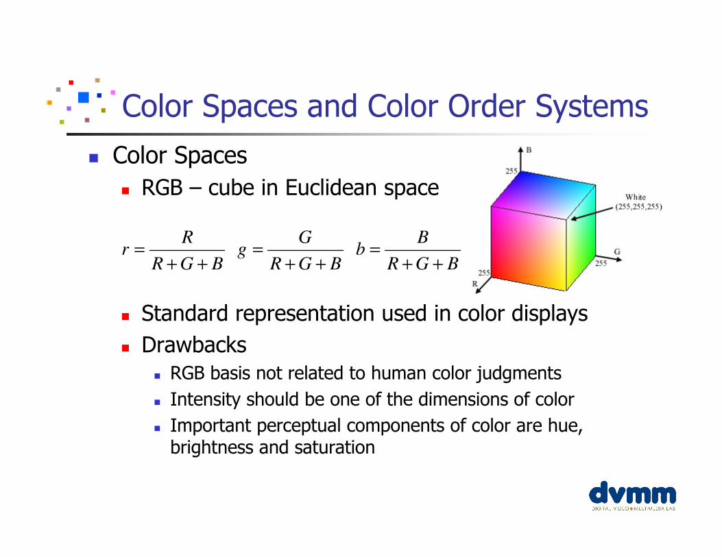
Color Spaces and Color Order Systems
� Color Spaces
� RGB – cube in Euclidean space
� Standard representation used in color displays
� Drawbacks
� RGB basis not related to human color judgments
� Intensity should be one of the dimensions of color
� Important perceptual components of color are hue, brightness and saturation
R G Br g b
R G B R G B R G B= = =
+ + + + + +
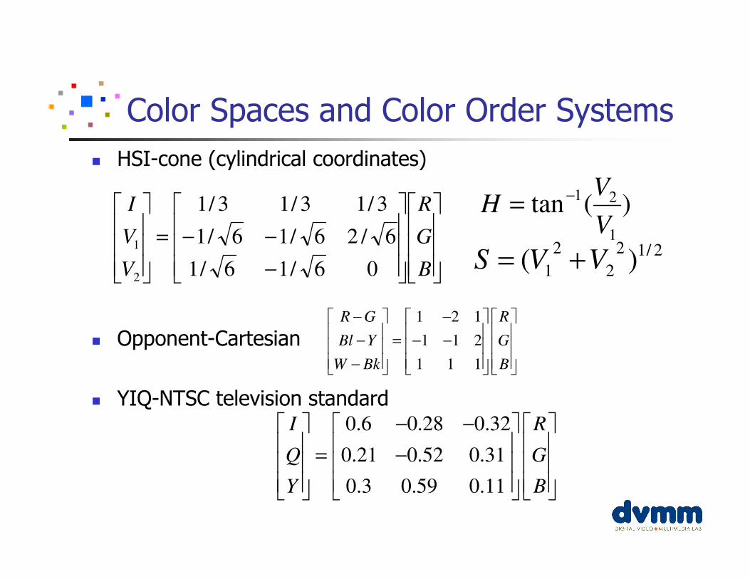
Color Spaces and Color Order Systems
� HSI-cone (cylindrical coordinates)
� Opponent-Cartesian
� YIQ-NTSC television standard0.6 0.28 0.32
0.21 0.52 0.31
0.3 0.59 0.11
I R
Q G
Y B
− −
= −
−
−−=
B
G
R
V
V
I
06/16/1
6/26/16/1
3/13/13/1
2
1
)(tan1
21
V
VH
−=
2/12
2
2
1 )( VVS +=
1 2 1
1 1 2
1 1 1
R G R
Bl Y G
W Bk B
− −
− = − − −
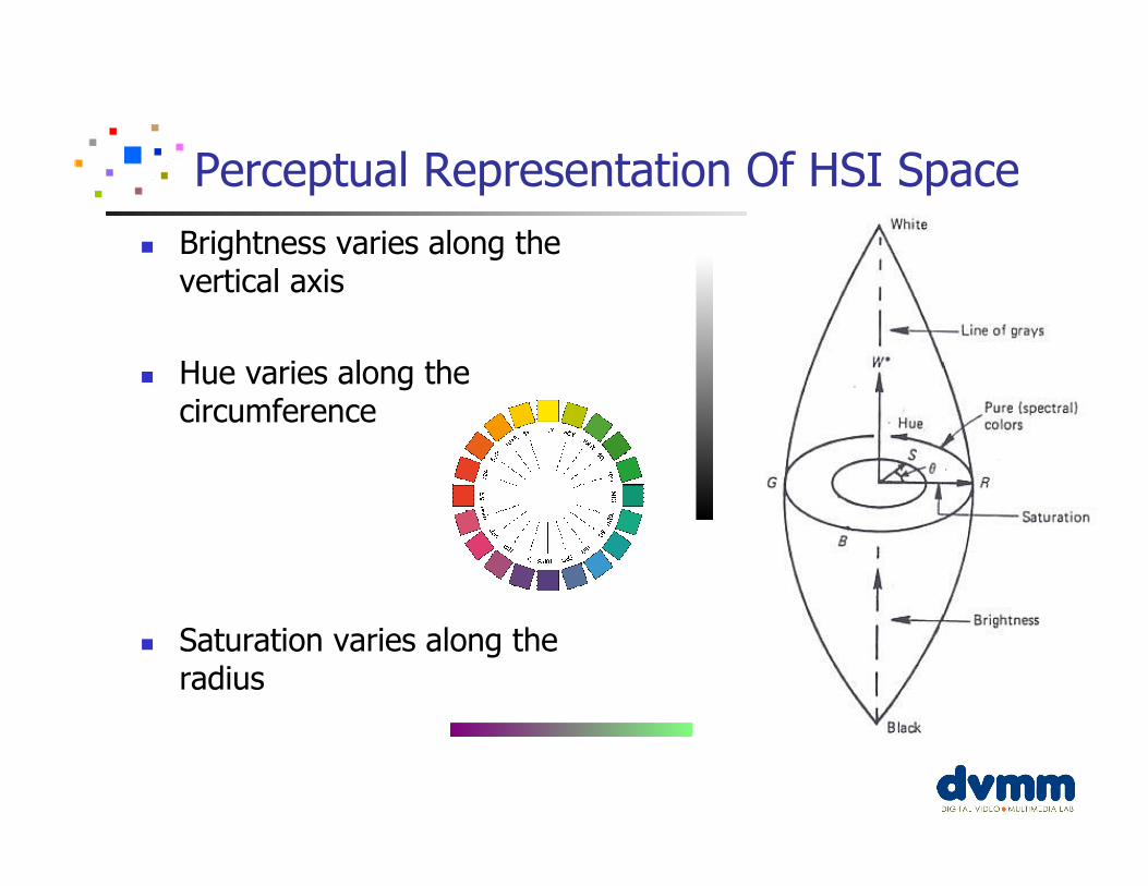
Perceptual Representation Of HSI Space
� Brightness varies along the vertical axis
� Hue varies along the circumference
� Saturation varies along the radius
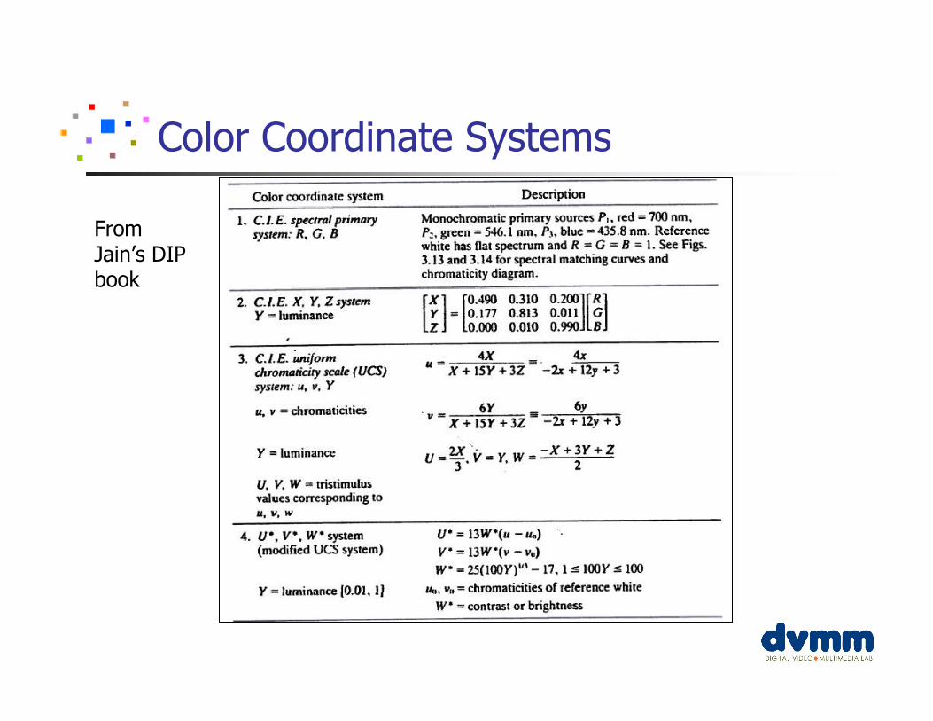
Color Coordinate Systems
From Jain’s DIP book
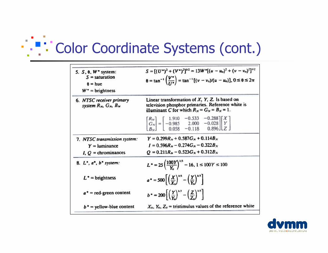
Color Coordinate Systems (cont.)
Color Space Quantization
� Why quantization: fewer numbers, less noise (?)� How many colors to keep
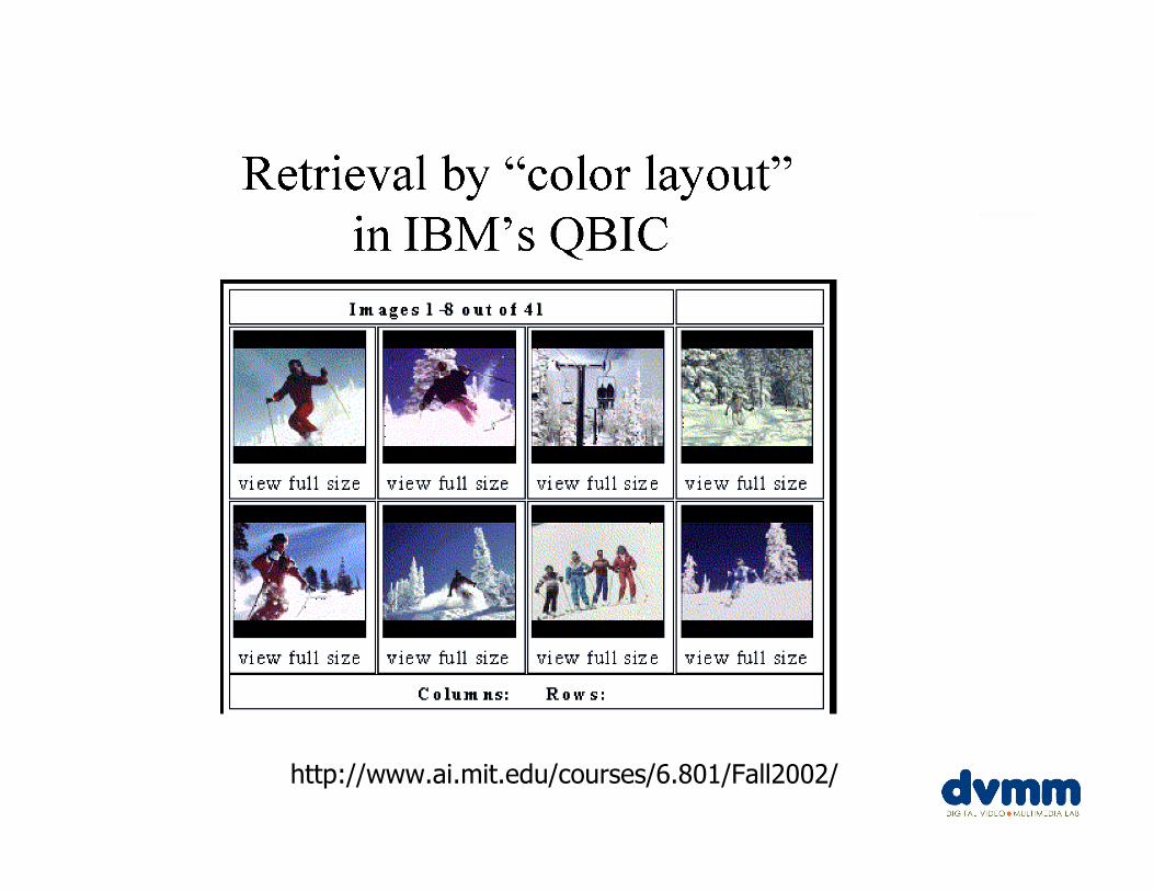
� IBM QBIC 1995 � 16M(RGB) �4096 (RGB) �64 (Munsell) colors
� Columbia U. VisualSEEK 1996 � 16M (RGB) � 166 (HSV) colors
� (18 Hue, 3 Sat, 3 Val, 4 Gray)
� Stricker and Orengo 1995 (Similarity of Color Images)� 16M (RGB) � 16 hues, 4 val, 4 sat = 128(HSV) colors� 16M (RGB) � 8 hues, 2 val, 2 sat = 32 (HSV) colors
� Independent quantization � each color dimension is quantized independently
� Joint quantization � color dimensions are quantized jointly
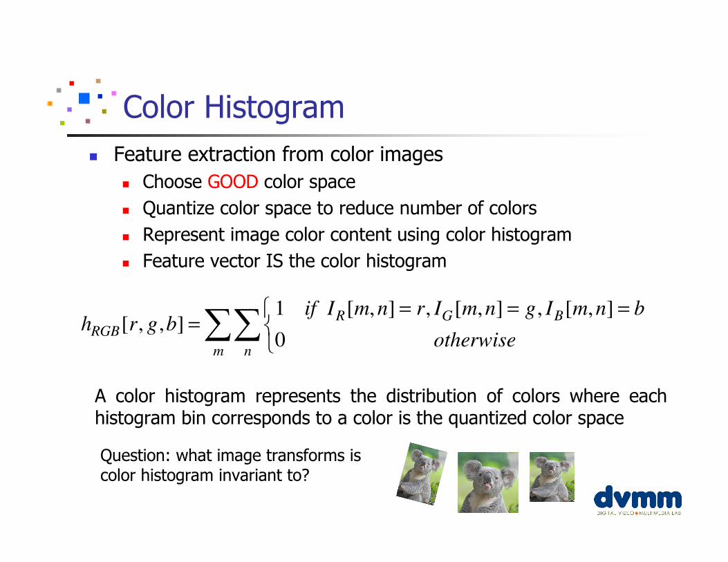
Color Histogram
� Feature extraction from color images
� Choose GOOD color space
� Quantize color space to reduce number of colors
� Represent image color content using color histogram
� Feature vector IS the color histogram
1 [ , ] , [ , ] , [ , ][ , , ]
0
R G BRGB
m n
if I m n r I m n g I m n bh r g b
otherwise
= = ==
∑∑
A color histogram represents the distribution of colors where each histogram bin corresponds to a color is the quantized color space
Question: what image transforms is color histogram invariant to?
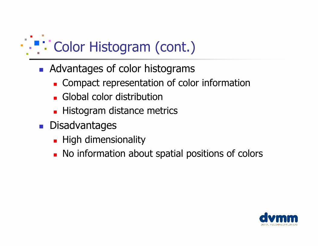
Color Histogram (cont.)
� Advantages of color histograms
� Compact representation of color information
� Global color distribution
� Histogram distance metrics
� Disadvantages
� High dimensionality
� No information about spatial positions of colors
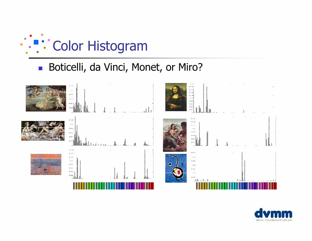
Color Histogram
� Boticelli, da Vinci, Monet, or Miro?
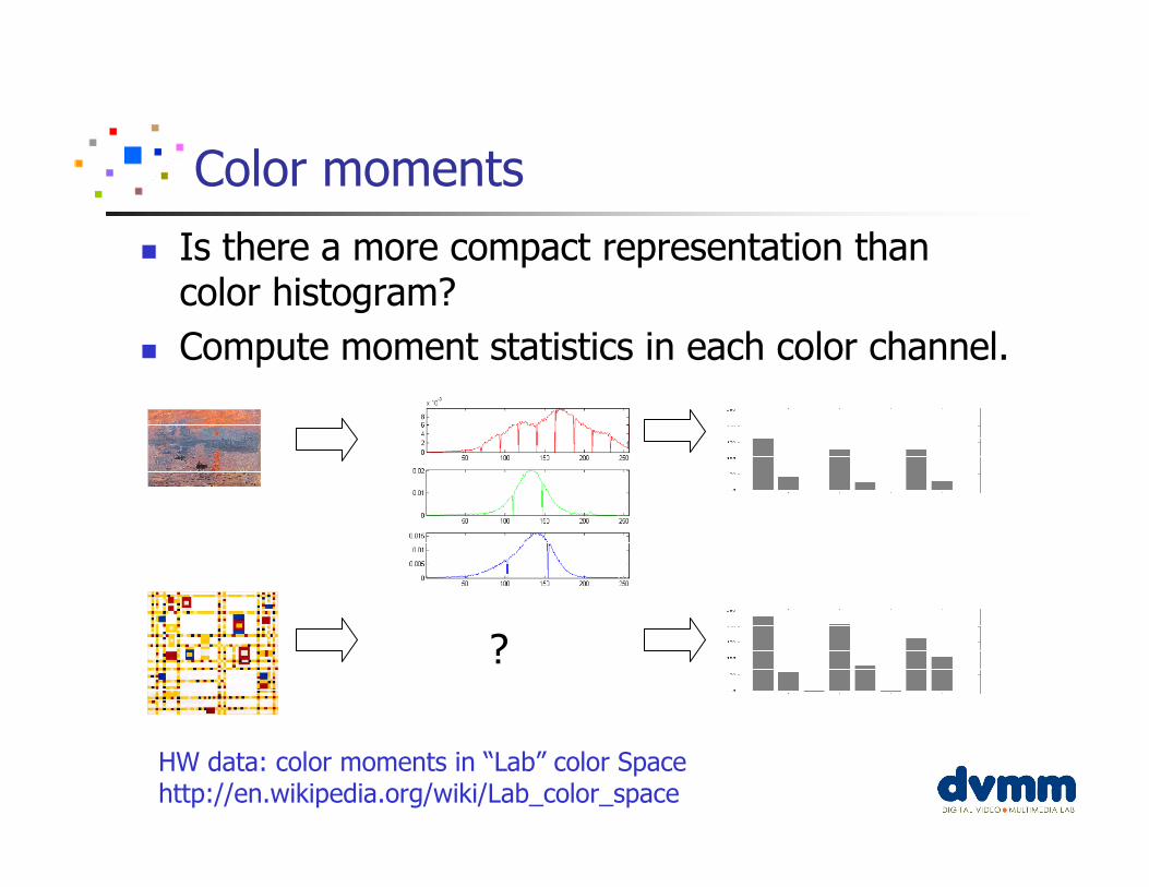
Color moments
� Is there a more compact representation than color histogram?
� Compute moment statistics in each color channel.
?
HW data: color moments in “Lab” color Space http://en.wikipedia.org/wiki/Lab_color_space
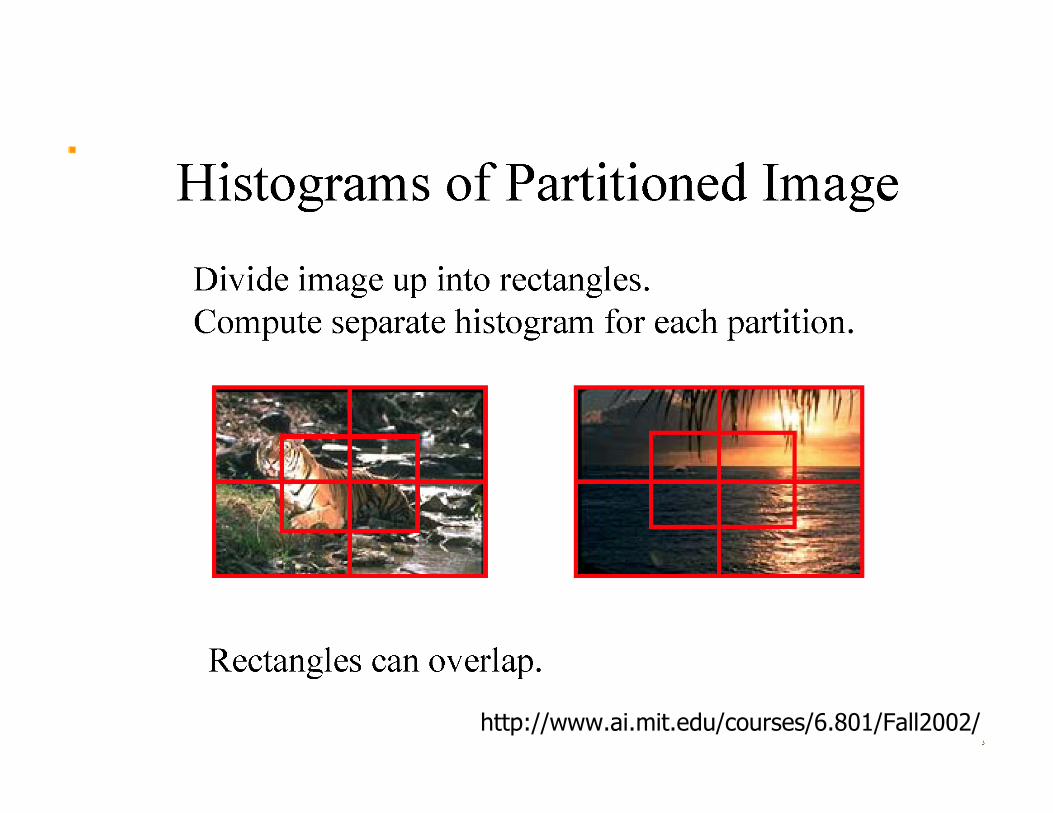
Localizing
http://www.ai.mit.edu/courses/6.801/Fall2002/
http://www.ai.mit.edu/courses/6.801/Fall2002/
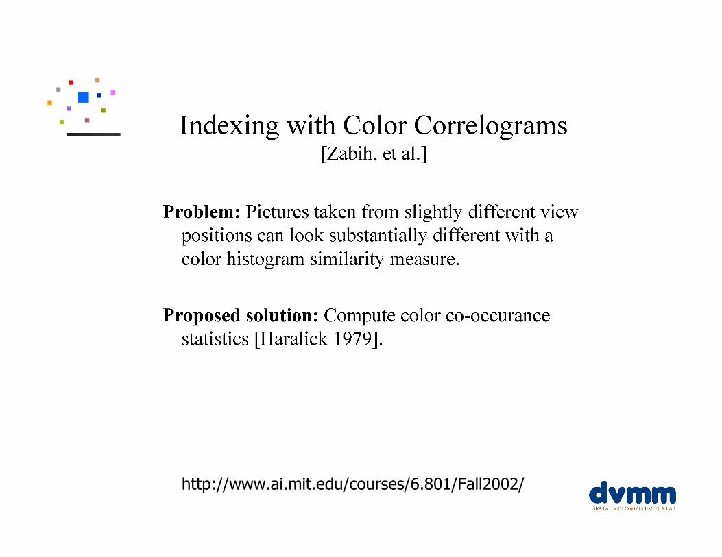
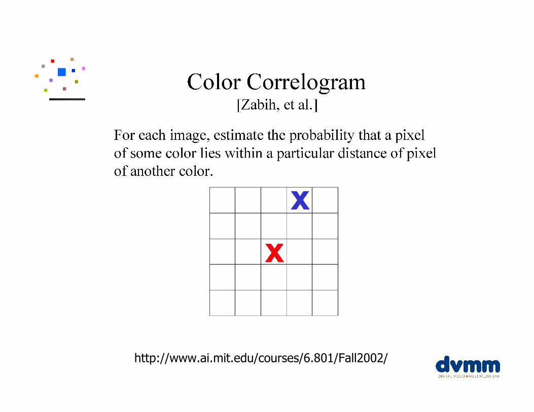
Color correlogram
http://www.ai.mit.edu/courses/6.801/Fall2002/
http://www.ai.mit.edu/courses/6.801/Fall2002/
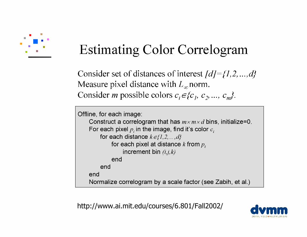
http://www.ai.mit.edu/courses/6.801/Fall2002/
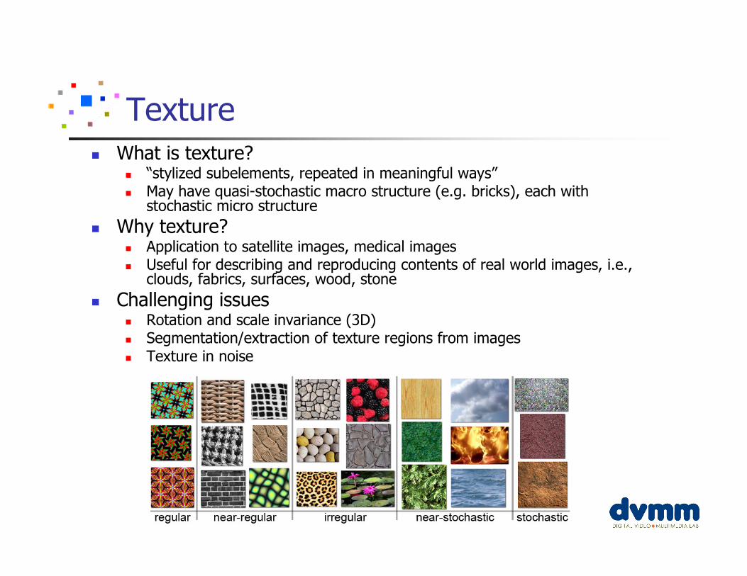
Texture� What is texture?
� “stylized subelements, repeated in meaningful ways”� May have quasi-stochastic macro structure (e.g. bricks), each with
stochastic micro structure
� Why texture?� Application to satellite images, medical images � Useful for describing and reproducing contents of real world images, i.e.,
clouds, fabrics, surfaces, wood, stone
� Challenging issues� Rotation and scale invariance (3D)� Segmentation/extraction of texture regions from images� Texture in noise
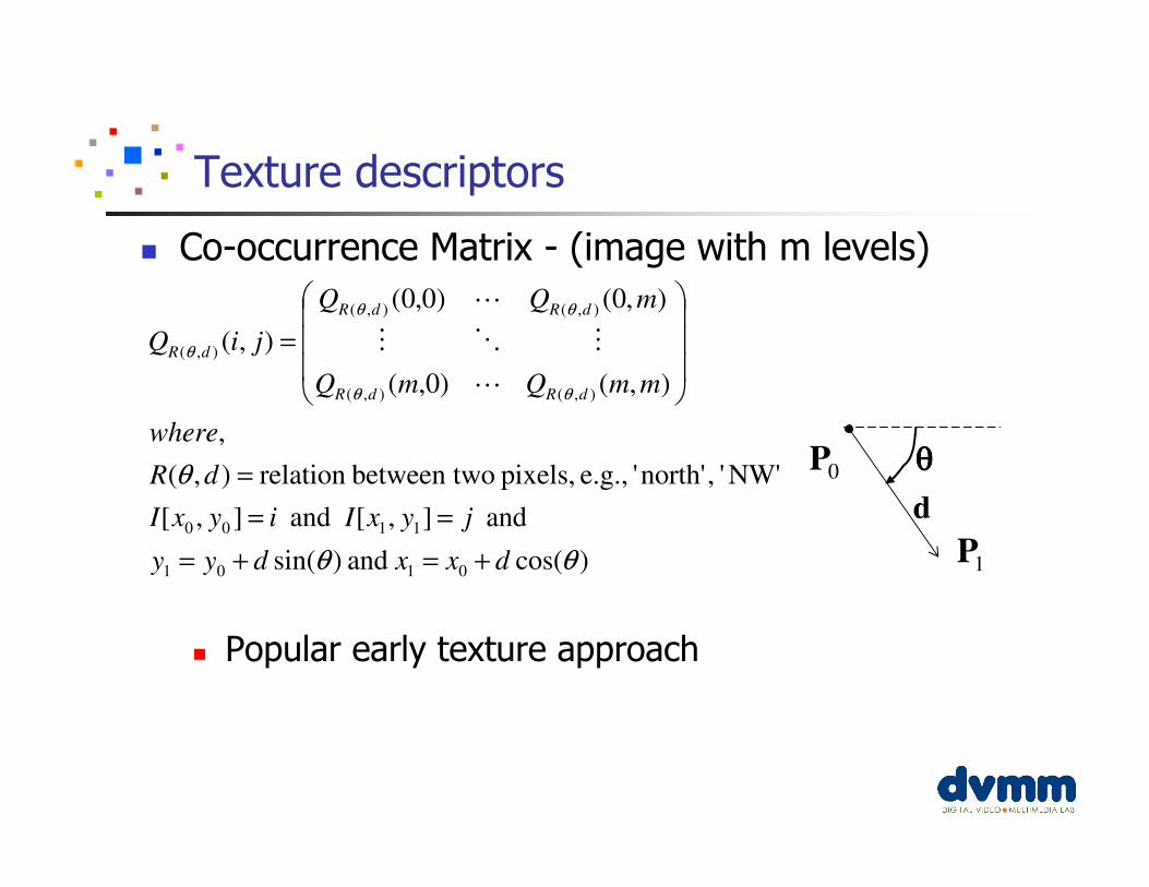
� Co-occurrence Matrix - (image with m levels)
� Popular early texture approach
Texture descriptors
)cos( and )sin(
and ],[ and ],[
NW'' ,north'' e.g., pixels, obetween twrelation ),(
,
),()0,(
),0()0,0(
),(
0101
1100
),(),(
),(),(
),(
θθ
θ
θθ
θθ
θ
dxxdyy
jyxIiyxI
dR
where
mmQmQ
mQQ
jiQ
dRdR
dRdR
dR
+=+=
==
=
=
⋯
⋮⋱⋮
⋯
0P
1P
d
θθθθ
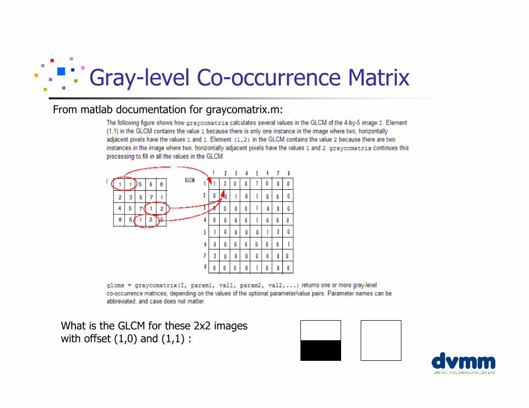
Gray-level Co-occurrence Matrix
What is the GLCM for these 2x2 images with offset (1,0) and (1,1) :
From matlab documentation for graycomatrix.m:
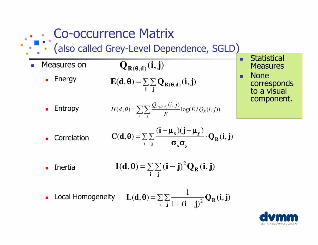
Co-occurrence Matrix(also called Grey-Level Dependence, SGLD)
� Measures on
� Energy
� Entropy
� Correlation
� Inertia
� Local Homogeneity
),(),( jiQ dR θθθθ
∑∑=i j
dR jiQdE ),(),( ),(θθθθθθθθ
)),(/log(),(
),(),(∑∑=
i j
R
dRjiQE
E
jiQdH
θθ
∑∑ ⋅−−
=i j
R
yx
yxjiQ
jidC ),(
))((),(
σσσσσσσσ
µµµµµµµµθθθθ
∑∑ −=i j
R jiQjidI ),()(),( 2θθθθ
∑∑−+
=i j
R jiQji
dL ),()(1
1),(
2θθθθ
� Statistical Measures
� None corresponds to a visual component.
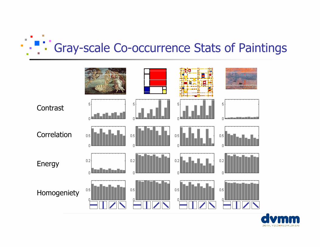
Gray-scale Co-occurrence Stats of Paintings
Energy
Contrast
Correlation
Homogeniety
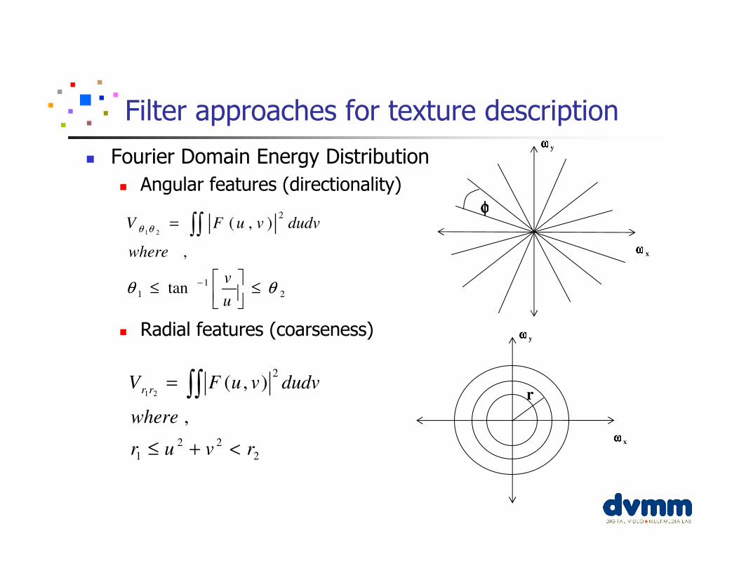
Filter approaches for texture description
� Fourier Domain Energy Distribution
� Angular features (directionality)
� Radial features (coarseness)
2
1
1
2
tan
,
),(21
θθ
θθ
≤
≤
=
−
∫∫
u
v
where
dudvvuFV
2
22
1
2
,
),(21
rvur
where
dudvvuFV rr
<+≤
= ∫∫
xωωωω
yωωωω
φφφφ
xωωωω
yωωωω
r
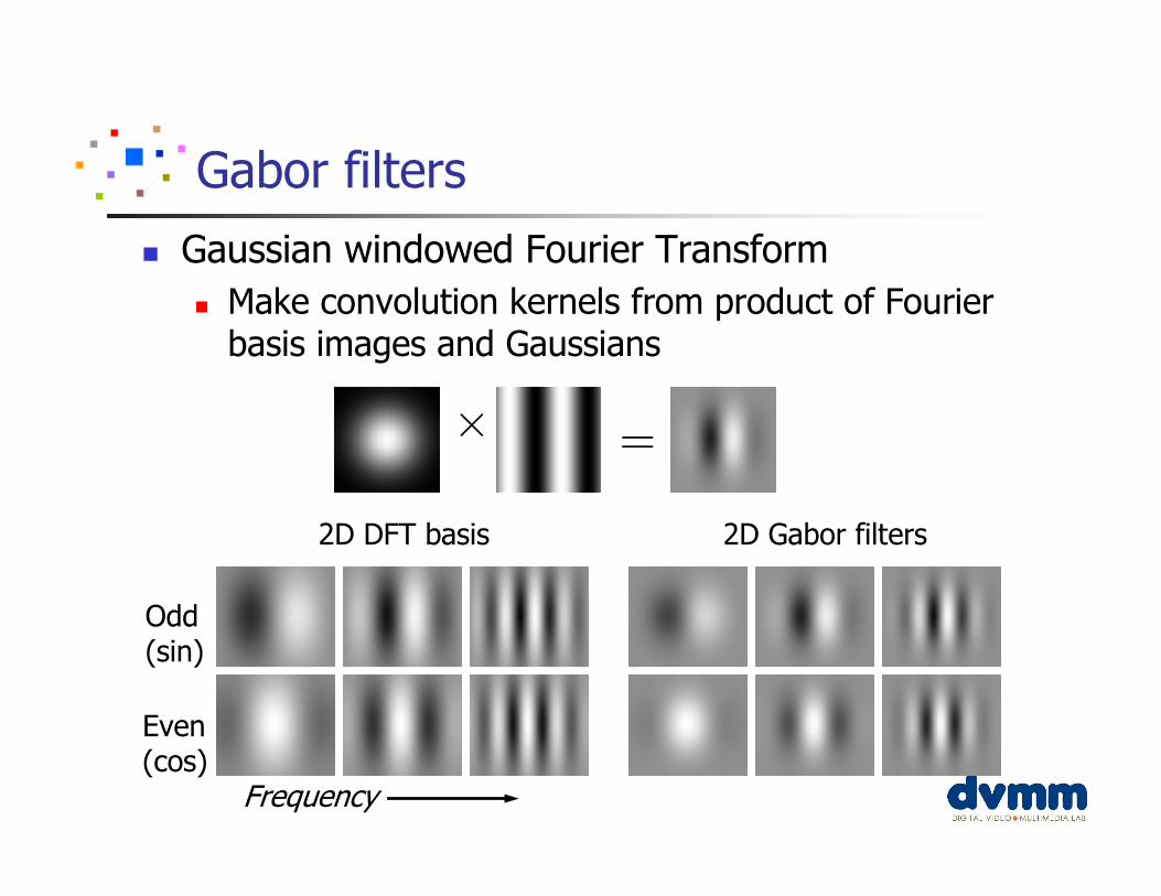
Gabor filters
� Gaussian windowed Fourier Transform
� Make convolution kernels from product of Fourier basis images and Gaussians
×=
Odd(sin)
Even(cos)
Frequency
2D DFT basis 2D Gabor filters
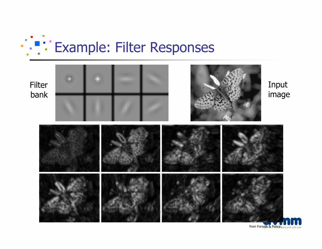
Example: Filter Responses
from Forsyth & Ponce
Filterbank
Inputimage
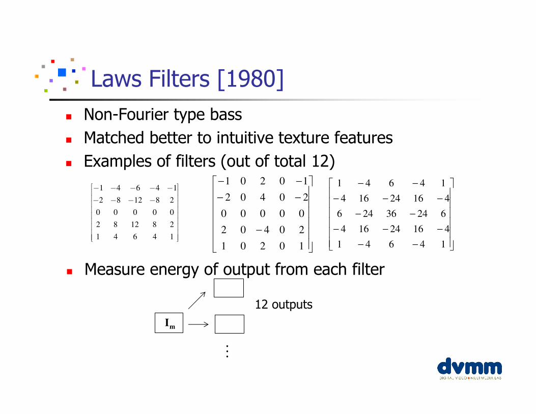
� Non-Fourier type bass
� Matched better to intuitive texture features
� Examples of filters (out of total 12)
Laws Filters [1980]
1 4 6 4 1
2 8 12 8 2
0 0 0 0 0
2 8 12 8 2
1 4 6 4 1
− − − − − − − − −
−
−−
−−
10201
20402
00000
20402
10201
−−
−−−
−−
−−−
−−
14641
41624164
62436246
41624164
14641
� Measure energy of output from each filter
mI
12 outputs
⋮
Tamura Texture
� Methods for approximating intuitive texture features
� Example: ‘Coarseness’, others: ‘contrast’, ‘directionality’� Step1: Compute averages at different scales, 1x1, 3x3, 5x5
pixels
� Step2: compute neighborhood difference at each scale
� Step 3: select the scale with the largest variation
� Step 4: compute the coarseness
k
BestL yxSEEEEyx 2) ( ), . . . , , max( determine ),( 21k ==∀
11
1 1
22
2
2 2
( , )( , ), ( , )
(2 1)
kk
k k
yx
k k
i x j y
f i jx y A x y
−−
− −
++
= − = −
∀ =+
∑ ∑
),2(),2() ( ),,( 11
, yxAyxAyxEyx k
k
k
khk
−− −−+=∀
∑∑= =
=m
j
n
i
BestCRS jiSMN
F1 1
),(1
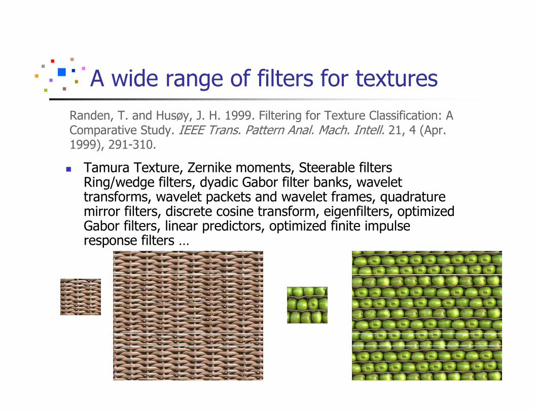
A wide range of filters for textures
� Tamura Texture, Zernike moments, Steerable filters Ring/wedge filters, dyadic Gabor filter banks, wavelet transforms, wavelet packets and wavelet frames, quadraturemirror filters, discrete cosine transform, eigenfilters, optimized Gabor filters, linear predictors, optimized finite impulse response filters …
Randen, T. and Husøy, J. H. 1999. Filtering for Texture Classification: A Comparative Study. IEEE Trans. Pattern Anal. Mach. Intell. 21, 4 (Apr. 1999), 291-310.
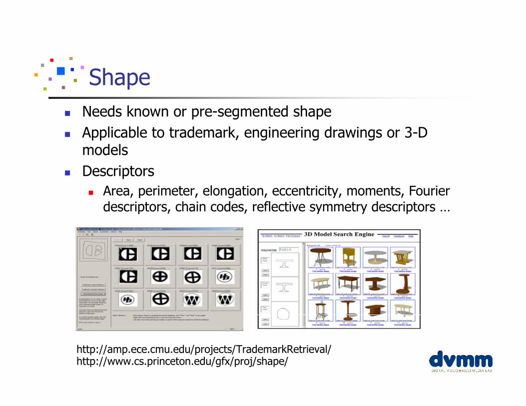
Shape
� Needs known or pre-segmented shape
� Applicable to trademark, engineering drawings or 3-D models
� Descriptors
� Area, perimeter, elongation, eccentricity, moments, Fourier descriptors, chain codes, reflective symmetry descriptors …
http://amp.ece.cmu.edu/projects/TrademarkRetrieval/http://www.cs.princeton.edu/gfx/proj/shape/
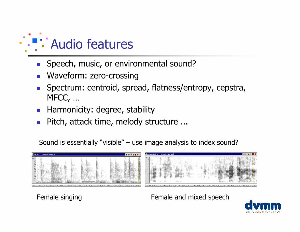
Audio features
� Speech, music, or environmental sound?
� Waveform: zero-crossing
� Spectrum: centroid, spread, flatness/entropy, cepstra, MFCC, …
� Harmonicity: degree, stability
� Pitch, attack time, melody structure ...
Sound is essentially “visible” – use image analysis to index sound?
Female singing Female and mixed speech
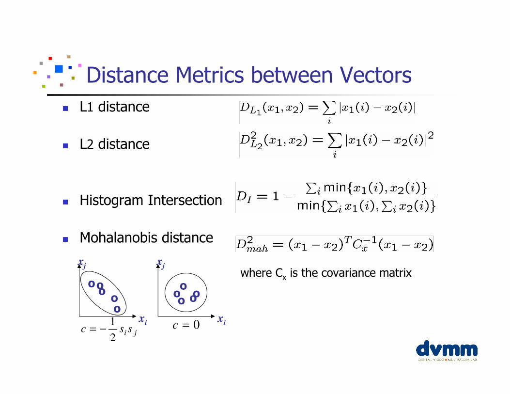
� L1 distance
� L2 distance
� Histogram Intersection
� Mohalanobis distance
Distance Metrics between Vectors
oooo
xi
xj
ooooo
xi
xj
o
1
2i jc s s= − 0c =
where Cx is the covariance matrix
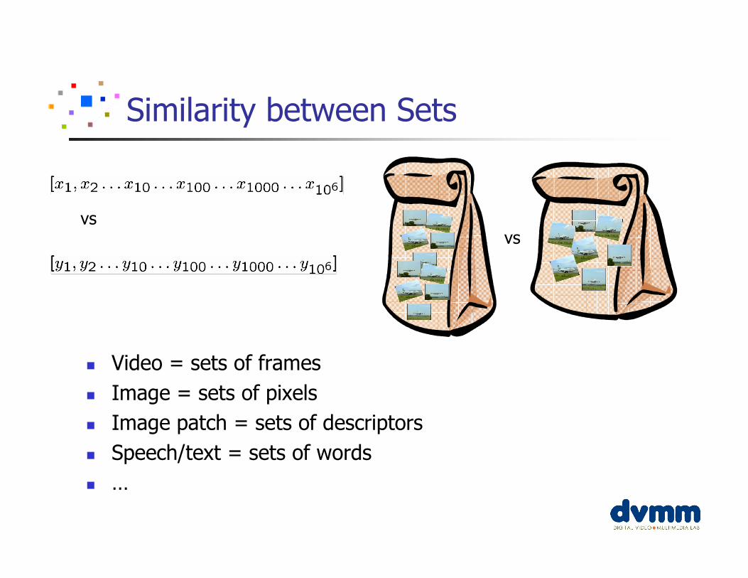
Similarity between Sets
� Video = sets of frames
� Image = sets of pixels
� Image patch = sets of descriptors
� Speech/text = sets of words
� …
vsvs
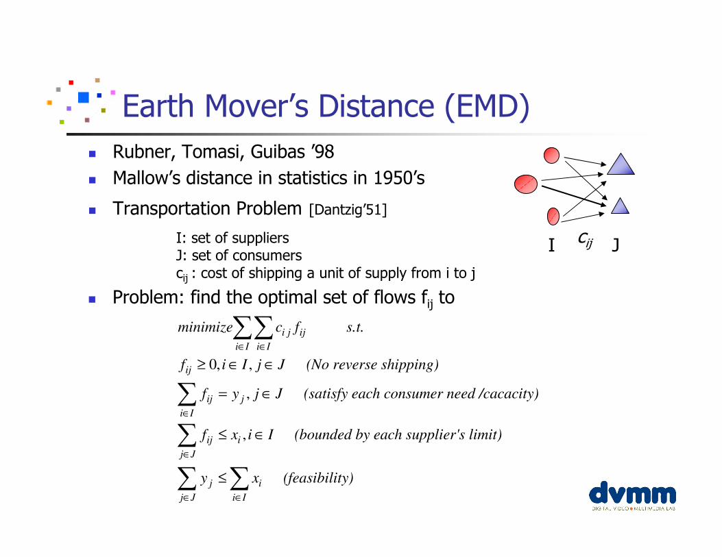
Earth Mover’s Distance (EMD)
� Rubner, Tomasi, Guibas ’98
� Mallow’s distance in statistics in 1950’s
� Transportation Problem [Dantzig’51]
I JcijI: set of suppliersJ: set of consumerscij : cost of shipping a unit of supply from i to j
� Problem: find the optimal set of flows fij to
0, ,
,
,
i j ij
i I i I
ij
ij j
i I
ij i
j J
j i
j J
minimize c f s.t.
f i I j J (No reverse shipping)
f y j J (satisfy each consumer need /cacacity)
f x i I (bounded by each supplier's limit)
y x (
∈ ∈
∈
∈
∈
≥ ∈ ∈
= ∈
≤ ∈
≤
∑∑
∑
∑
∑i I
feasibility)
∈
∑
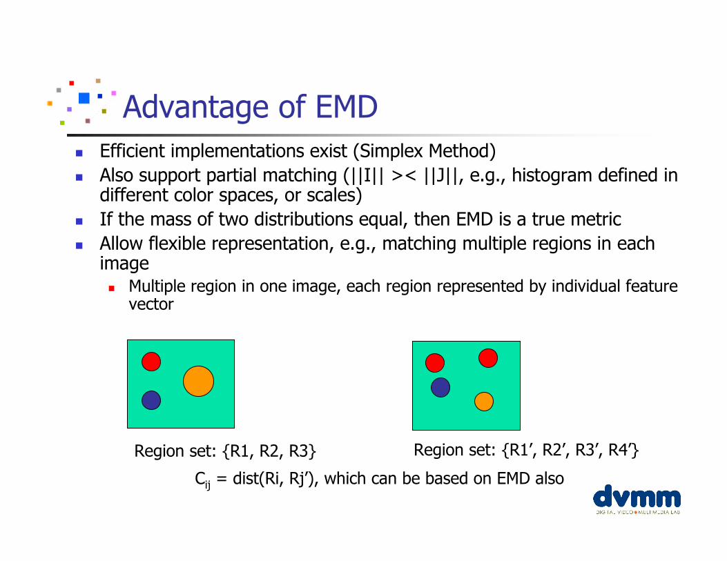
Advantage of EMD
� Efficient implementations exist (Simplex Method)
� Also support partial matching (||I|| >< ||J||, e.g., histogram defined in different color spaces, or scales)
� If the mass of two distributions equal, then EMD is a true metric
� Allow flexible representation, e.g., matching multiple regions in each image� Multiple region in one image, each region represented by individual feature
vector
Region set: {R1, R2, R3} Region set: {R1’, R2’, R3’, R4’}
Cij = dist(Ri, Rj’), which can be based on EMD also
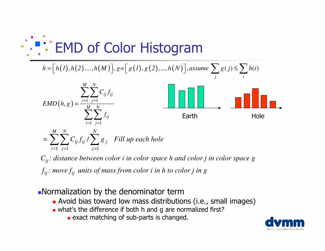
EMD of Color Histogram
( ) ( ) ( ) ( ) ( ) ( )
( )1 1
1 1
, ,..., , , ,..., , ( ) ( )
,
j i
M N
ij ij
i j
M N
ij
i j
h h 1 h 2 h M g= g 1 g 2 h N assume g j h i
C f
EMD h g
f
= =
= =
= ≤
=
∑ ∑
∑∑
∑∑ Earth Hole
1 1 1
/
M N N
ij ij j
i j j
ij
ij ij
= C f g Fill up each hole
C : distance between color i in color space h and color j in color space g
f : move f units of mass from color i in h to color j in g
= = =
∑∑ ∑
�Normalization by the denominator term� Avoid bias toward low mass distributions (i.e., small images)� what’s the difference if both h and g are normalized first?
� exact matching of sub-parts is changed.
� Question
� When to use which metric?
� Can various metrics be used together?
� How do we combine them?
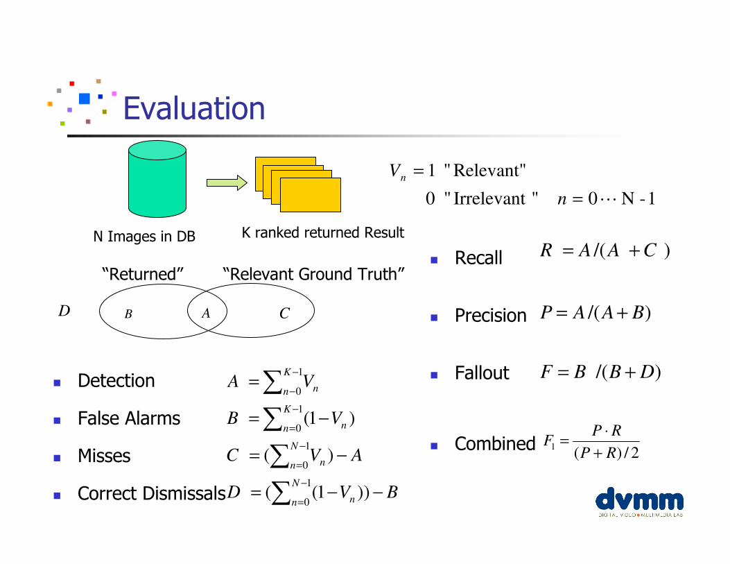
Evaluation
� Detection
� False Alarms
� Misses
� Correct Dismissals
)/(
)/(
)/(
DBBF
BAAP
CAAR
+=
+=
+=
1-N0 "Irrelevant" 0
Relevant"" 1
⋯=
=
n
Vn
BVD
AVC
VB
VA
N
n n
N
n n
K
n n
K
n n
−−=
−=
−=
=
∑
∑
∑
∑
−
=
−
=
−
=
−
−
))1((
)(
)1(
1
0
1
0
1
0
1
0
N Images in DB K ranked returned Result
� Recall
� Precision
� Fallout
� Combined2/)(
1RP
RPF
+
⋅=
D B CA
“Returned” “Relevant Ground Truth”
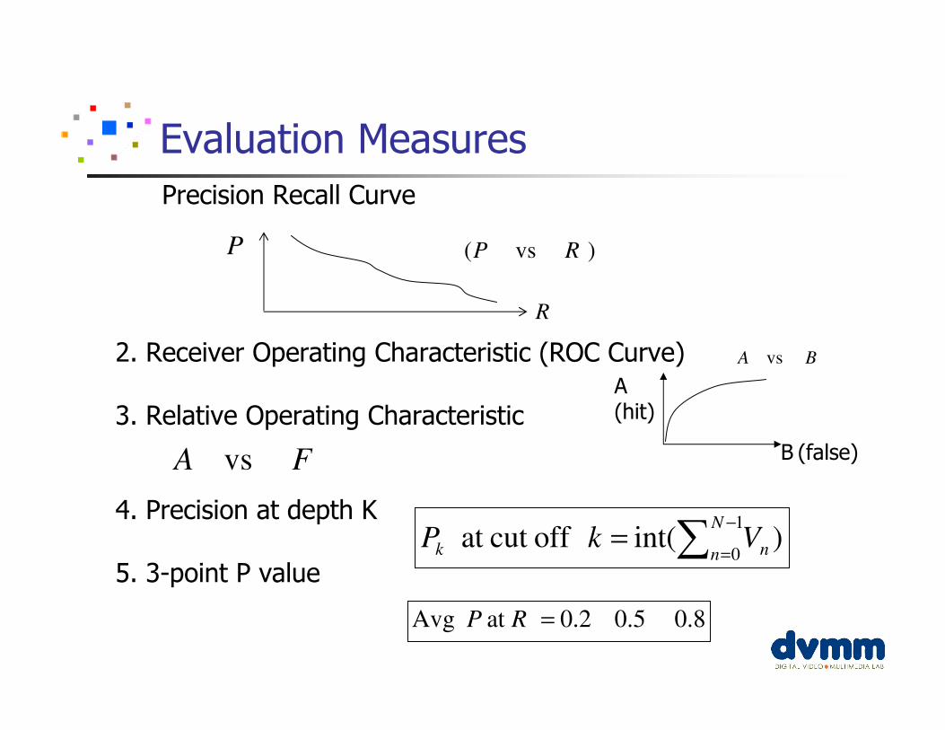
Evaluation Measures
Precision Recall Curve
2. Receiver Operating Characteristic (ROC Curve)
3. Relative Operating Characteristic
4. Precision at depth K
5. 3-point P value
) vs( RPP
R
BA vs
FA vs
)int( offcut at 1
0∑−
==
N
n nk VkP
0.8 0.5 .20at Avg =RP
A(hit)
B (false)
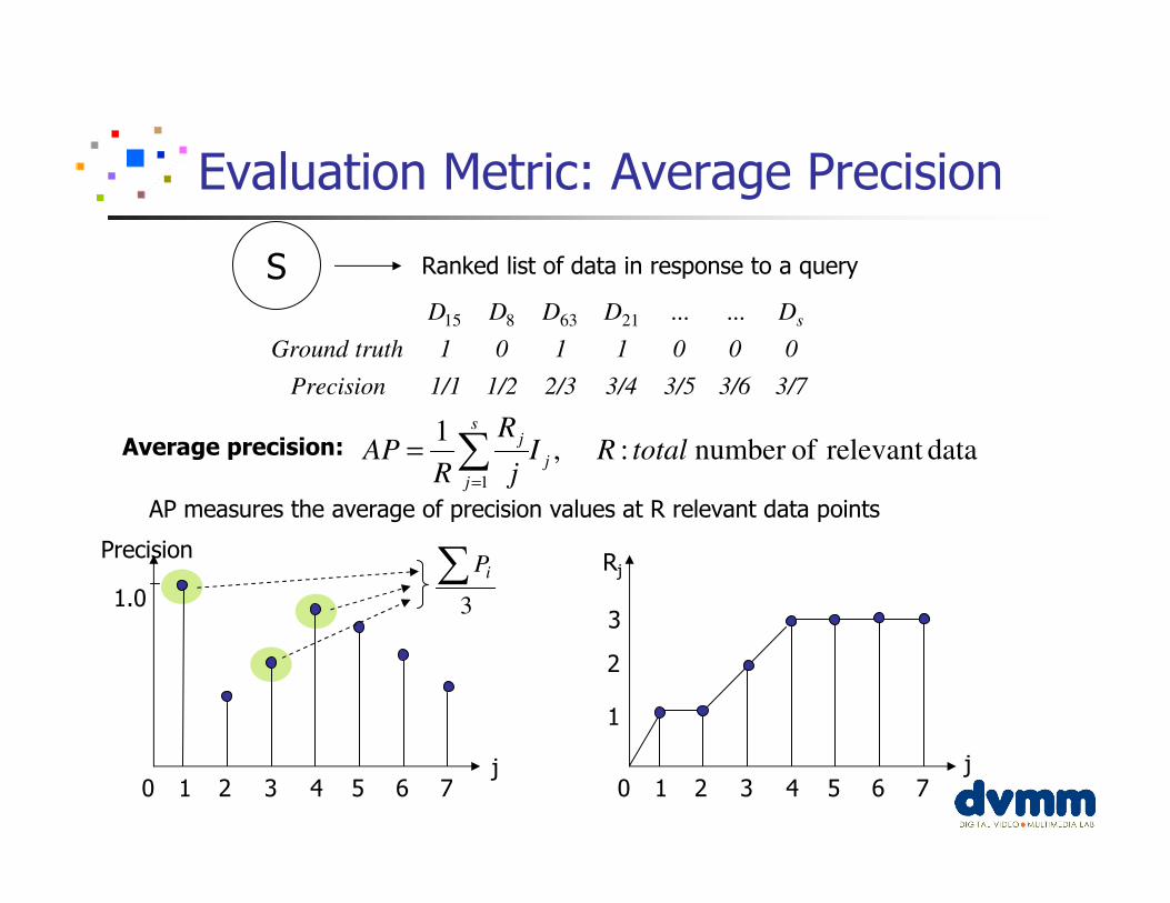
Evaluation Metric: Average Precision
S Ranked list of data in response to a query
3/73/63/53/42/31/21/1Precision
0001101truth Ground
DDDDD s......2163815
Average precision: datarelevant ofnumber : ,1
1
totalRIj
R
RAP j
s
j
j∑=
=
0 1 2 3 4 5 6 7
Precision
j
3
∑ iP
AP measures the average of precision values at R relevant data points
0 1 2 3 4 5 6 7
Rj
j
1
2
31.0
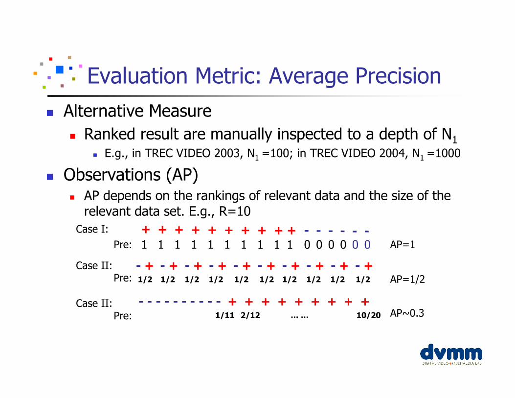
Evaluation Metric: Average Precision
� Alternative Measure
� Ranked result are manually inspected to a depth of N1
� E.g., in TREC VIDEO 2003, N1 =100; in TREC VIDEO 2004, N1 =1000
� Observations (AP)� AP depends on the rankings of relevant data and the size of the
relevant data set. E.g., R=10
Case I: + + + + + + + + + - - - - --+Pre: 1 1 1 1 1 1 1 1 1 0 0 0 0 001 AP=1
Case II: - +Pre: 1/2 AP=1/2
- + - + - + - + - + - + - + - + - +1/2 1/2 1/2 1/2 1/2 1/2 1/2 1/2 1/2
Case II: Pre:
- - - --- - - -- + + + + + + + + +1/11 2/12 10/20… … AP~0.3
Evaluation Metric: Average Precision
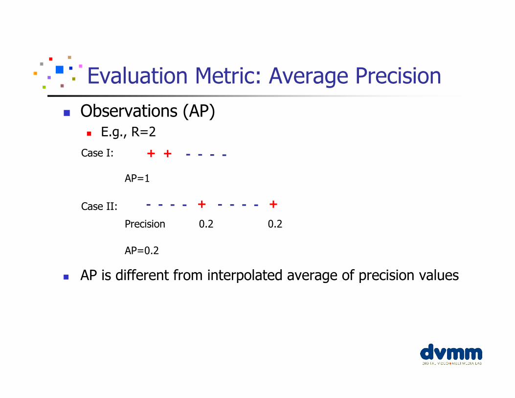
� Observations (AP)� E.g., R=2
� AP is different from interpolated average of precision values
Case I: + + - - - -
AP=1
Case II: - - - - + - - - - +
AP=0.2
Precision 0.2 0.2
HW #1
……
Paper Review and Demo
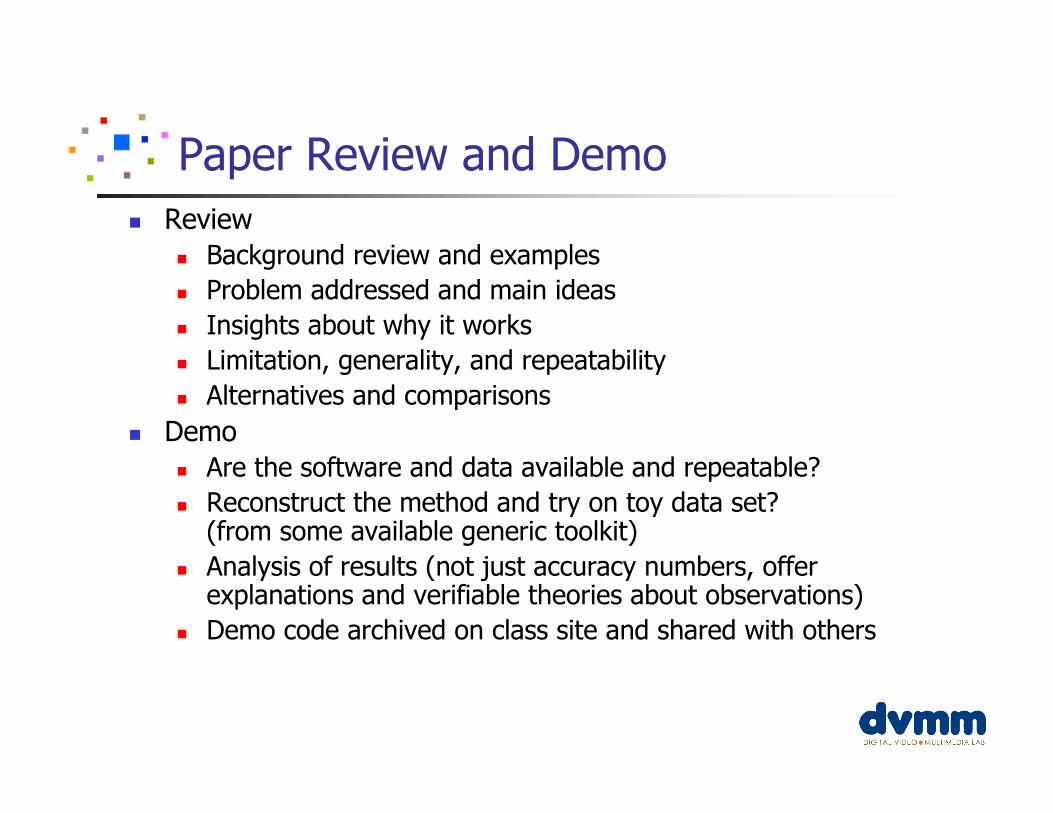
� Review
� Background review and examples
� Problem addressed and main ideas
� Insights about why it works
� Limitation, generality, and repeatability
� Alternatives and comparisons
� Demo
� Are the software and data available and repeatable?
� Reconstruct the method and try on toy data set?(from some available generic toolkit)
� Analysis of results (not just accuracy numbers, offer explanations and verifiable theories about observations)
� Demo code archived on class site and shared with others
Paper review and demo
� Sample work schedule
� Week 1: understand paper, review and research
� Week 2: simulate a toy problem using available data set and tools
� Week 3: prepare presentation
� Each student discusses paper and demos with Eric, Prof. Chang or me two weeks before class.
� Upload the slide and codes to CourseWorks before class
� Presentation
� 30 mins each paper (including demo)
� We will provide additional materials about the subject.

Choose your paper/topic now!
StudentsPaper
Presentation
10/29/07
StudentsPaper
Presentation
10/8/07
� Four weeks of paper presentation
� 4 papers each week… starting three weeks from now!
� Email us of your choices by Tuesday!
……
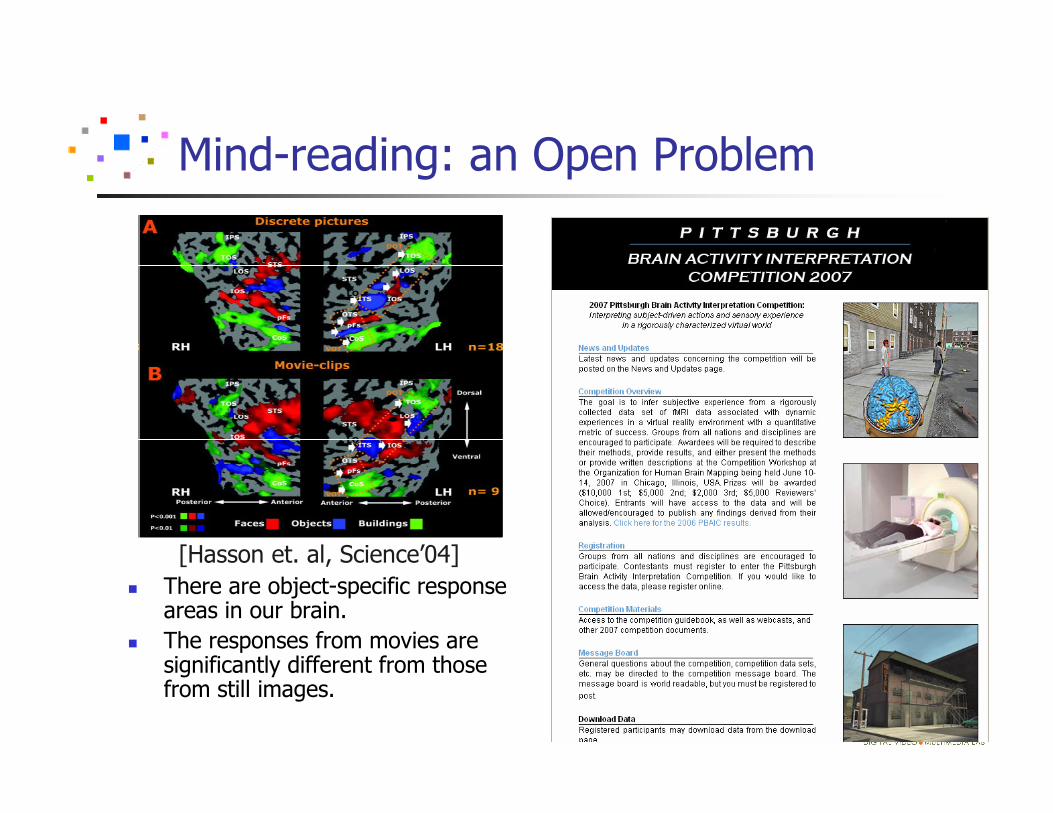
Mind-reading: an Open Problem
� There are object-specific response areas in our brain.
� The responses from movies are significantly different from those from still images.
[Hasson et. al, Science’04]