Embed Size (px)
Citation preview

Chapter 5: Optimum Receiver for Binary Data Transmission
EE456 – Digital CommunicationsProfessor Ha Nguyen
September 2015
EE456 – Digital Communications 1
Chapter 5: Optimum Receiver for Binary Data Transmission
Block Diagram of Binary Communication Systems
������ ���� ���� ���� ����������������
������ ��������������������������
( )tm { }kb 10 ( )k s t= ↔b
21 ( )k s t= ↔b
ˆ ( )tm { }ˆkb ( )tr
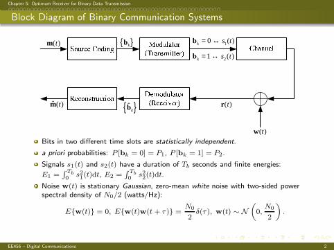
( )twBits in two different time slots are statistically independent.
a priori probabilities: P [bk = 0] = P1, P [bk = 1] = P2.
Signals s1(t) and s2(t) have a duration of Tb seconds and finite energies:
E1 =∫ Tb0
s21(t)dt, E2 =∫ Tb0
s22(t)dt.
Noise w(t) is stationary Gaussian, zero-mean white noise with two-sided powerspectral density of N0/2 (watts/Hz):
E{w(t)} = 0, E{w(t)w(t + τ)} =N0
2δ(τ), w(t) ∼ N
(
0,N0
2
)
.
EE456 – Digital Communications 2
Chapter 5: Optimum Receiver for Binary Data Transmission
������ ��� !" �#$!!�%&���%$'��()�$!*+ ''��,
-�+���%$'��(.��� /��,.���!*'���' �!
( )tm { }kb 10 ( )k s t= ↔b
21 ( )k s t= ↔b
ˆ ( )tm { }ˆkb ( )tr
( )tw
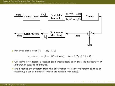
Received signal over [(k − 1)Tb, kTb]:
r(t) = si(t− (k − 1)Tb) +w(t), (k − 1)Tb ≤ t ≤ kTb.
Objective is to design a receiver (or demodulator) such that the probability ofmaking an error is minimized.
Shall reduce the problem from the observation of a time waveform to that ofobserving a set of numbers (which are random variables).
EE456 – Digital Communications 3
Chapter 5: Optimum Receiver for Binary Data Transmission
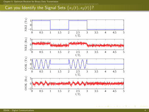
Can you Identify the Signal Sets {s1(t), s2(t)}?
0 0.5 1 1.5 2 2.5 3 3.5 4 4.5 5−1
0
1
t/Tb
NRZ(T
x)
0 0.5 1 1.5 2 2.5 3 3.5 4 4.5 5−5
0
5
t/Tb
NRZ(R
x)
0 0.5 1 1.5 2 2.5 3 3.5 4 4.5 5−1
0
1
t/Tb
OOK
(Tx)
0 0.5 1 1.5 2 2.5 3 3.5 4 4.5 5−5
0
5
t/Tb
OOK
(Rx)
EE456 – Digital Communications 4
Chapter 5: Optimum Receiver for Binary Data Transmission
Geometric Representation of Signals s1(t) and s2(t) (I)
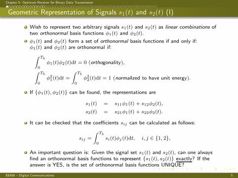
Wish to represent two arbitrary signals s1(t) and s2(t) as linear combinations oftwo orthonormal basis functions φ1(t) and φ2(t).
φ1(t) and φ2(t) form a set of orthonormal basis functions if and only if:φ1(t) and φ2(t) are orthonormal if:
∫ Tb
0φ1(t)φ2(t)dt = 0 (orthogonality),
∫ Tb
0φ21(t)dt =
∫ Tb
0φ22(t)dt = 1 (normalized to have unit energy).
If {φ1(t), φ2(t)} can be found, the representations are
s1(t) = s11φ1(t) + s12φ2(t),
s2(t) = s21φ1(t) + s22φ2(t).
It can be checked that the coefficients sij can be calculated as follows:
sij =
∫ Tb
0si(t)φj (t)dt, i, j ∈ {1, 2},
An important question is: Given the signal set s1(t) and s2(t), can one alwaysfind an orthonormal basis functions to represent {s1(t), s2(t)} exactly? If theanswer is YES, is the set of orthonormal basis functions UNIQUE?
EE456 – Digital Communications 5
Chapter 5: Optimum Receiver for Binary Data Transmission
Geometric Representation of Signals s1(t) and s2(t) (II)
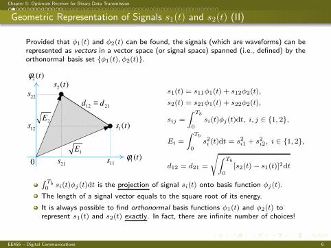
Provided that φ1(t) and φ2(t) can be found, the signals (which are waveforms) can berepresented as vectors in a vector space (or signal space) spanned (i.e., defined) by theorthonormal basis set {φ1(t), φ2(t)}.
)(1 tφ
)(1 ts
)(2 ts)(2 tφ
0 11s
21s
12s
22s
12 21d d=
2E
1E
s1(t) = s11φ1(t) + s12φ2(t),
s2(t) = s21φ1(t) + s22φ2(t),
sij =
∫ Tb
0si(t)φj(t)dt, i, j ∈ {1, 2},
Ei =
∫ Tb
0s2i (t)dt = s2i1 + s2i2, i ∈ {1, 2},
d12 = d21 =
√∫ Tb
0[s2(t) − s1(t)]2dt
∫ Tb0
si(t)φj (t)dt is the projection of signal si(t) onto basis function φj(t).
The length of a signal vector equals to the square root of its energy.
It is always possible to find orthonormal basis functions φ1(t) and φ2(t) torepresent s1(t) and s2(t) exactly. In fact, there are infinite number of choices!
EE456 – Digital Communications 6
Chapter 5: Optimum Receiver for Binary Data Transmission
Gram-Schmidt Procedure
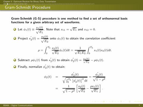
Gram-Schmidt (G-S) procedure is one method to find a set of orthonormal basisfunctions for a given arbitrary set of waveforms.
1 Let φ1(t) ≡ s1(t)√
E1
. Note that s11 =√E1 and s12 = 0.
2 Project s′
2(t) =s2(t)√
E2
onto φ1(t) to obtain the correlation coefficient:
ρ =
∫ Tb
0
s2(t)√E2
φ1(t)dt =1√
E1E2
∫ Tb
0s1(t)s2(t)dt.
3 Subtract ρφ1(t) from s′
2(t) to obtain φ′
2(t) =s2(t)√
E2− ρφ1(t).
4 Finally, normalize φ′
2(t) to obtain:
φ2(t) =φ
′
2(t)√∫ Tb0
[φ
′
2(t)]2
dt=
φ′
2(t)√
1− ρ2
=1
√
1− ρ2
[s2(t)√E2
− ρs1(t)√E1
]
.
EE456 – Digital Communications 7
Chapter 5: Optimum Receiver for Binary Data Transmission
Gram-Schmidt Procedure: Summary
)(2 ts
)(1 ts
22s
21s1E0
2E
1( )tφ
2( )s t′
1( )tρφ
2( )tφ
α21d
1 cos( ) 1ρ α− ≤ = ≤
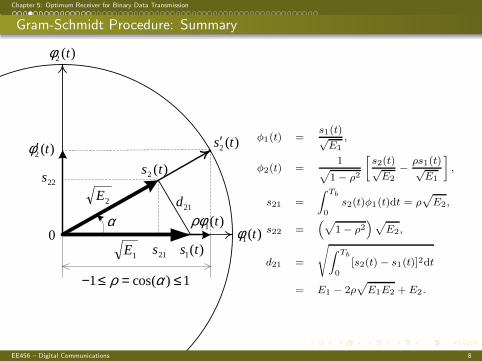
2( )tφ′φ1(t) =
s1(t)√E1
,
φ2(t) =1
√1− ρ2
[s2(t)√E2
− ρs1(t)√E1
]
,
s21 =
∫ Tb
0s2(t)φ1(t)dt = ρ
√
E2,
s22 =(√
1− ρ2)√
E2,
d21 =
√∫ Tb
0[s2(t) − s1(t)]2dt
= E1 − 2ρ√
E1E2 +E2.
EE456 – Digital Communications 8
Chapter 5: Optimum Receiver for Binary Data Transmission
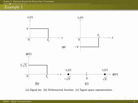
Example 1
0
)(2 ts
0bT
V−
0
)(1 ts
V
0bT
123
4
)(1 tφ
bT1
0bT
567
)(1 tφ0
)(1 ts)(2 ts
E− E
89:
(a) Signal set. (b) Orthonormal function. (c) Signal space representation.
EE456 – Digital Communications 9
Chapter 5: Optimum Receiver for Binary Data Transmission
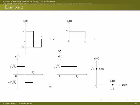
Example 2
V−
;
)(1 ts
V
0bT ;
)(2 ts
V
0bT
<=>
?
)(1 tφ
bT1
0bT
bT1−
?
)(2 tφ
0bT
bT1
@AB )(1 tφ0
)(1 ts
)(2 tsE
E
)(2 tφ
EE456 – Digital Communications 10

Chapter 5: Optimum Receiver for Binary Data Transmission
Example 3
C
)(2 ts
0bT
V−
C
)(1 ts
V
0bT
V
α
)(1 tφ0
)(1 ts
)(2 ts
),(2 αφ t
0=α
2bT=α
ρα , increasing
( )0,E( )0,E−
E
DDEF
GGHI
−2
3,
2
EE
4bTα =
ρ =1
E
∫Tb
0
s2(t)s1(t)dt
=1
V 2Tb
[
V 2α − V 2(Tb − α)]
=2α
Tb
− 1
EE456 – Digital Communications 11

Chapter 5: Optimum Receiver for Binary Data Transmission
Example 4
J
)(2 ts
0bT
V3
J
)(1 ts
V
0bT 2bT
KLM
N
)(1 tφ
bT1
0bT
N
)(2 tφ
0bT
2bT
bT
3−
bT
3
OPQ
EE456 – Digital Communications 12

Chapter 5: Optimum Receiver for Binary Data Transmission
2( )tφ
0
1( )s t
2( )s t
32E
1( )tφ
o602E E
ρ =1
E
∫Tb
0
s2(t)s1(t)dt =2
E
∫Tb/2
0
(
2√3
Tb
V t
)
V dt =
√3
2,
φ2(t) =1
(1 − 34 )
12
[s2(t)√
E− ρ
s1(t)√E
]
=2
√E
[
s2(t) −√3
2s1(t)
]
,
s21 =
√3
2
√E, s22 =
1
2
√E.
d21 =
[∫ Tb
0
[s2(t) − s1(t)]2dt
] 12
=
√(
2 −√3)
E.
EE456 – Digital Communications 13

Chapter 5: Optimum Receiver for Binary Data Transmission
Example 5
)(1 tφ0
)(1 ts
)(2 ts
E
)(2 tφ
1−==
ρπθ
0
23
==
ρπθ
0
2
==
ρπθ
2locus of ( ) as
varies from 0 to 2 .
s t θπ
θ
s1(t) =√E
√
2
Tb
cos(2πfct),
s2(t) =√E
√
2
Tb
cos(2πfct + θ).
where fc = k2Tb
, k an integer.
EE456 – Digital Communications 14
Chapter 5: Optimum Receiver for Binary Data Transmission
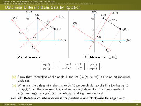
Obtaining Different Basis Sets by Rotation
)(1 tφ
)(1 ts
)(2 ts)(2 tφ
)(1 tφ
θ
)(2 tφ
0 11s
21s
12s
22s
)(1 tφ
)(1 ts
)(2 ts
)(2 tφ)(1 tφ
θ
)(2 tφ
0 11s
21s
12s
22s
11 21s s=11
s
21s
22s
12s
11 21s s=
12s
22s
[φ1(t)
φ2(t)
]
=
[cos θ sin θ
− sin θ cos θ
] [φ1(t)φ2(t)
]
.
(a) Show that, regardless of the angle θ, the set {φ1(t), φ2(t)} is also an orthonormalbasis set.
(b) What are the values of θ that make φ1(t) perpendicular to the line joining s1(t)to s2(t)? For these values of θ, mathematically show that the components of
s1(t) and s2(t) along φ1(t), namely s11 and s21, are identical.
Remark: Rotating counter-clockwise for positive θ and clock-wise for negative θ.
EE456 – Digital Communications 15

Chapter 5: Optimum Receiver for Binary Data Transmission
Example: Rotating {φ1(t), φ2(t)} by θ = 60◦ to Obtain {φ1(t), φ2(t)}
[φ1(t)
φ2(t)
]
=
[cos θ sin θ
− sin θ cos θ
] [φ1(t)φ2(t)
]
⇒{
φ1(t) = cos θ × φ1(t) + sin θ × φ2(t)
φ2(t) = − sin θ × φ1(t) + cos θ × φ2(t)
00 5.0 5.0 1
1( )tφ
1
2
)31( +
2
)31( −2
)31( −
2
)31( +−
)(2 tφ
0
)(1 tφ
01
1
1 1
1−
5.0
2( )tφ
EE456 – Digital Communications 16
Chapter 5: Optimum Receiver for Binary Data Transmission
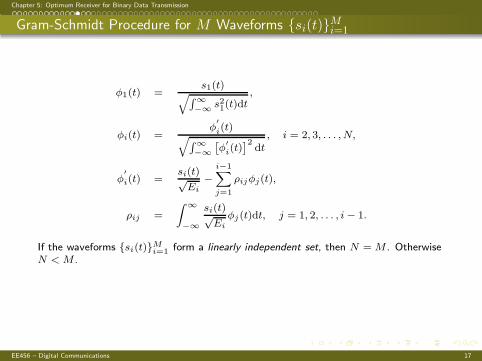
Gram-Schmidt Procedure for M Waveforms {si(t)}Mi=1
φ1(t) =s1(t)
√∫∞−∞ s21(t)dt
,
φi(t) =φ
′
i(t)√∫∞−∞
[φ
′
i(t)]2
dt, i = 2, 3, . . . , N,
φ′
i(t) =si(t)√Ei
−i−1∑
j=1
ρijφj(t),
ρij =
∫ ∞
−∞
si(t)√Ei
φj(t)dt, j = 1, 2, . . . , i− 1.
If the waveforms {si(t)}Mi=1 form a linearly independent set, then N = M . OtherwiseN < M .
EE456 – Digital Communications 17

Chapter 5: Optimum Receiver for Binary Data Transmission
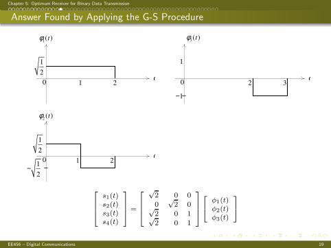
Example: Find a Basis Set for the Following M = 4 Waveforms
)(1 ts
0
1
1
3( )s t
02 2 3
)(2 ts
1
1−
0
1
1
4( )s t
02 2 3
1
1−1−
EE456 – Digital Communications 18
Chapter 5: Optimum Receiver for Binary Data Transmission
Answer Found by Applying the G-S Procedure
1( )tφ
0
1
2
1
3( )tφ
02 2 3
2( )tφ
1
1−
0 1 2
1
2
1
2−
s1(t)s2(t)s3(t)s4(t)
=
√2 0 0
0√2 0√
2 0 1√2 0 1
φ1(t)φ2(t)φ3(t)
EE456 – Digital Communications 19
Chapter 5: Optimum Receiver for Binary Data Transmission
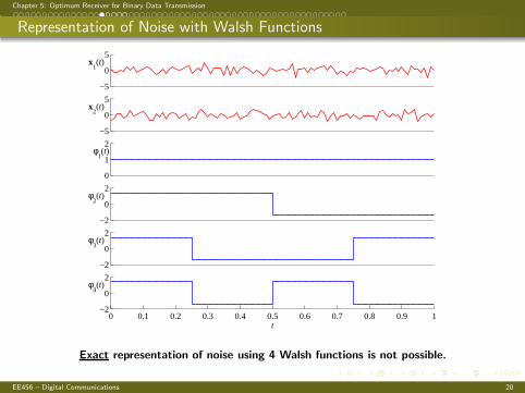
Representation of Noise with Walsh Functions
−5
0
5x
1(t)
−5
0
5x
2(t)
0
1
2φ
1(t)
−2
0
2φ
2(t)
−2
0
2φ
3(t)
0 0.1 0.2 0.3 0.4 0.5 0.6 0.7 0.8 0.9 1−2
0
2φ
4(t)
t
Exact representation of noise using 4 Walsh functions is not possible.
EE456 – Digital Communications 20
Chapter 5: Optimum Receiver for Binary Data Transmission
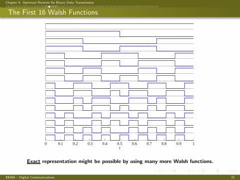
The First 16 Walsh Functions
0 0.1 0.2 0.3 0.4 0.5 0.6 0.7 0.8 0.9 1t
Exact representation might be possible by using many more Walsh functions.
EE456 – Digital Communications 21
Chapter 5: Optimum Receiver for Binary Data Transmission
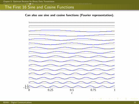
The First 16 Sine and Cosine Functions
Can also use sine and cosine functions (Fourier representation).
0 0.25 0.5 0.75 1−1.5
1.5
t
EE456 – Digital Communications 22
Chapter 5: Optimum Receiver for Binary Data Transmission
Representation of Noise
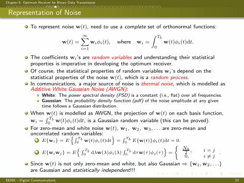
To represent noise w(t), need to use a complete set of orthonormal functions:
w(t) =∞∑
i=1
wiφi(t), where wi =
∫ Tb
0w(t)φi(t)dt.
The coefficients wi’s are random variables and understanding their statisticalproperties is imperative in developing the optimum receiver.
Of course, the statistical properties of random variables wi’s depend on thestatistical properties of the noise w(t), which is a random process.In communications, a major source of noise is thermal noise, which is modelled asAdditive White Gaussian Noise (AWGN):
White: The power spectral density (PSD) is a constant (i.e., flat) over all frequencies.Gaussian: The probability density function (pdf) of the noise amplitude at any giventime follows a Gaussian distribution.
When w(t) is modelled as AWGN, the projection of w(t) on each basis function,
wi =∫ Tb0
w(t)φi(t)dt, is a Gaussian random variable (this can be proved).
For zero-mean and white noise w(t), w1, w2, w3, . . . are zero-mean anduncorrelated random variables:
1 E{wi} = E{∫ Tb
0 w(t)φi(t)dt}
=∫ Tb0 E{w(t)}φi(t)dt = 0.
2 E{wiwj} = E{∫ Tb
0 dλw(λ)φi(λ)∫ Tb0 dτw(τ)φj(τ)
}
=
{N02 , i = j
0, i 6= j.
Since w(t) is not only zero-mean and white, but also Gaussian ⇒ {w1,w2, . . .}are Gaussian and statistically independent!!!
EE456 – Digital Communications 23

Chapter 5: Optimum Receiver for Binary Data Transmission
Need to Review Probability Theory &Random Processes – Chapter 3 Slides
EE456 – Digital Communications 24
Chapter 5: Optimum Receiver for Binary Data Transmission
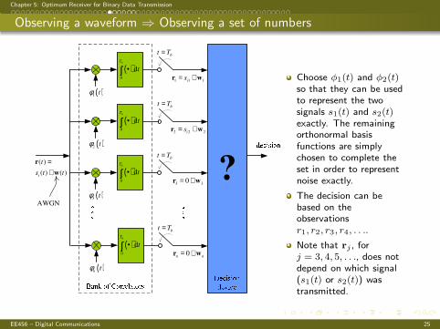
Observing a waveform ⇒ Observing a set of numbers
( )ntφ
bt T=
0n n
= +r w
( )0
dbT
t•∫
( )3tφ
bt T=
3 30= +r w
( )0
dbT
t•∫
( )2tφ
bt T=
2 2 2is= +r w
( )0
dbT
t•∫
( )1tφ
bt T=
1 1 1is= +r w
( )0
dbT
t•∫
( )
( ) ( )i
t
s t t
=+
r
w
AWGN
Choose φ1(t) and φ2(t)so that they can be usedto represent the twosignals s1(t) and s2(t)exactly. The remainingorthonormal basisfunctions are simplychosen to complete theset in order to representnoise exactly.
The decision can bebased on theobservationsr1, r2, r3, r4, . . ..
Note that rj , forj = 3, 4, 5, . . ., does notdepend on which signal(s1(t) or s2(t)) wastransmitted.
EE456 – Digital Communications 25
Chapter 5: Optimum Receiver for Binary Data Transmission
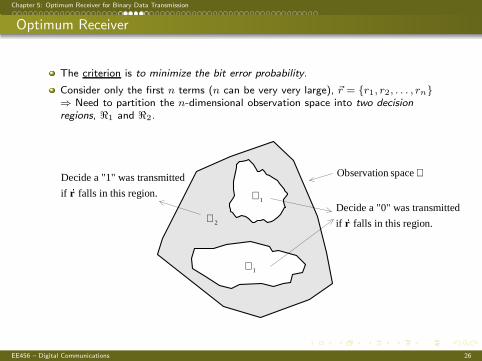
Optimum Receiver
The criterion is to minimize the bit error probability.
Consider only the first n terms (n can be very very large), ~r = {r1, r2, . . . , rn}⇒ Need to partition the n-dimensional observation space into two decisionregions, ℜ1 and ℜ2.
1ℜ
1ℜ
2ℜ
ℜ space nObservatioDecide a "1" was transmitted
if falls in this region.rR
Decide a "0" was transmitted
if falls in this region.rR
EE456 – Digital Communications 26
Chapter 5: Optimum Receiver for Binary Data Transmission
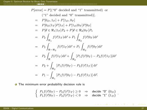
P [error] = P [(“0” decided and “1” transmitted) or
(“1” decided and “0” transmitted)].
= P [0D, 1T ] + P [1D, 0T ]
= P [0D|1T ]P [1T ] + P [1D|0T ]P [0T ]
= P [~r ∈ ℜ1|1T ]P2 + P [~r ∈ ℜ2|0T ]P1
= P2
∫
ℜ1
f(~r|1T )d~r + P1
∫
ℜ2
f(~r|0T )d~r
= P2
∫
ℜ−ℜ2
f(~r|1T )d~r + P1
∫
ℜ2
f(~r|0T )d~r
= P2
∫
ℜf(~r|1T )d~r +
∫
ℜ2
[P1f(~r|0T )− P2f(~r|1T )]d~r
= P2 +
∫
ℜ2
[P1f(~r|0T )− P2f(~r|1T )] d~r
= P1 −∫
ℜ1
[P1f(~r|0T )− P2f(~r|1T )] d~r.
The minimum error probability decision rule is
{P1f(~r|0T )− P2f(~r|1T ) ≥ 0 ⇒ decide “0” (0D)P1f(~r|0T )− P2f(~r|1T ) < 0 ⇒ decide “1” (1D)
.
EE456 – Digital Communications 27
Chapter 5: Optimum Receiver for Binary Data Transmission
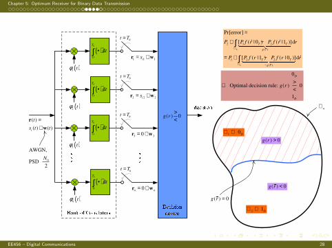
( )ntφ
bt T=
0n n= +r w
( )0
dbT
t•∫
( )3tφ
bt T=
3 30= +r w
( )0
dbT
t•∫
( )2 tφ
bt T=
2 2 2is= +r w
( )0
dbT
t•∫
( )1tφ
bt T=
1 1 1is= +r w
( )0
dbT
t•∫
( )
( ) ( )i
t
s t t
=+
r
w
0
AWGN,
PSD 2
N
2
1
2 1 2
( )
1 2 2
( )
Pr[error]
[ ( | 0 ) ( |1 )]d
[ ( |1 ) ( | 0 )]d
T T
g r
T T
g r
P P f r P f r r
P P f r P f r r
ℜ
ℜ −
=
+ −
= + −
∫
∫
1 0Dℜ ⇔
21
Dℜ ⇔
( ) 0g r <
( ) 0g r >
( ) 0g r =
nℜ
( ) 0g r><
0
Optimal decision rule: ( ) 0
1
D
D
g r>⇒<
EE456 – Digital Communications 28
Chapter 5: Optimum Receiver for Binary Data Transmission
Equivalently,
f(~r|1T )f(~r|0T )
1D
R0D
P1P2
. (1)
The expressionf(~r|1T )f(~r|0T )
is called the likelihood ratio.
The decision rule in (1) was derived without specifying any statistical propertiesof the noise process w(t).
Simplified decision rule when the noise w(t) is zero-mean, white and Gaussian:
(r1 − s11)2 + (r2 − s12)21D
R0D
(r1 − s21)2 + (r2 − s22)2 +N0ln(P1P2
)
.
For the special case of P1 = P2 (signals are equally likely):
(r1 − s11)2 + (r2 − s12)21D
R0D
(r1 − s21)2 + (r2 − s22)2.
⇒ minimum-distance receiver!
EE456 – Digital Communications 29
Chapter 5: Optimum Receiver for Binary Data Transmission
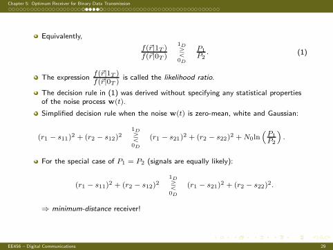
Minimum-Distance Receiver
(r1 − s11)2 + (r2 − s12)
2
︸ ︷︷ ︸
d21
1D
R0D
(r1 − s21)2 + (r2 − s22)
2
︸ ︷︷ ︸
d22
d21
1D
R0D
d22
)(1 tφ
0
)(1 ts
)(2 ts
)(2 tφ
),( 1211 ss
),( 2221 ss
)( Choose 2 ts )( Choose 1 ts 1r
2r
( )r t
( )1 2,r r 1d
2d
EE456 – Digital Communications 30
Chapter 5: Optimum Receiver for Binary Data Transmission
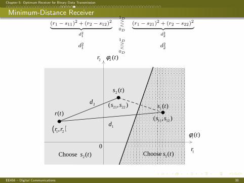
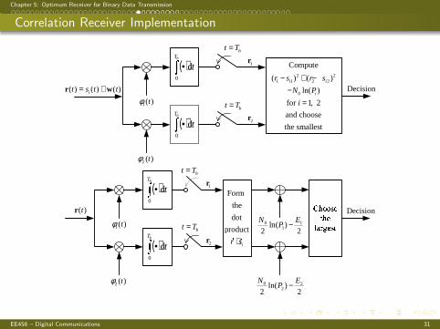
Correlation Receiver Implementation
( )S •bT
t0
d
)(2 tφ
( )T •bT
t0
d
)(1 tφ
bTt =
bTt =
Decision
1r
2r
( ) ( ) ( )it s t t= +r w
2 21 1 2 2
0
Compute
( ) ( )
ln( )
for 1, 2
and choose
the smallest
i i
i
r s r s
N P
i
− + −−
=
( )U •bT
t0
d
)(2 tφ
( )V •bT
t0
d
)(1 tφ
bTt =
bTt =
DecisionWXYYZ[\X[
]^_`[Z\2)ln(
21
10 E
PN −
2)ln(
22
20 E
PN −
( )tr
1r
2r
Form
the
dot
product
ir s⋅a a
EE456 – Digital Communications 31
Chapter 5: Optimum Receiver for Binary Data Transmission
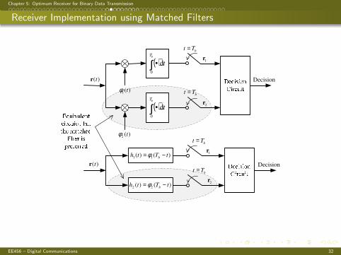
Receiver Implementation using Matched Filters
( )∫ •bT
t0
d
)(2 tφ
( )∫ •bT
t0
d
)(1 tφ
bTt =
bTt =
)()( 22 tTth b −= φ
)()( 11 tTth b −= φ
bTt =
bTt =Decision
( )tr
1r
2r
( )tr
1r
2r
Decision
EE456 – Digital Communications 32

Chapter 5: Optimum Receiver for Binary Data Transmission
Example 5.6
b
)(2 ts
0b
)(1 ts
0 5.0
5.0
1
15.0
5.1
2−cde
f
)(1 tφ
1
0 1f
)(2 tφ
5.00
1−
1
1
ghi
EE456 – Digital Communications 33
Chapter 5: Optimum Receiver for Binary Data Transmission
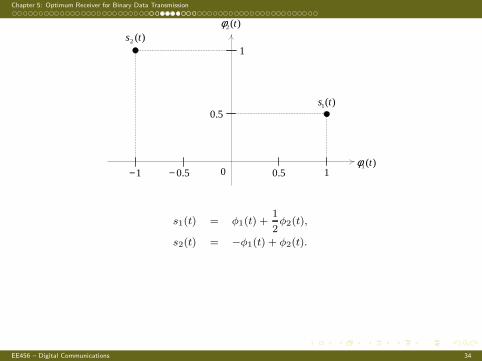
)(1 tφ0
)(1 ts
)(2 ts)(2 tφ
5.0−
5.0
5.0 11−
1
s1(t) = φ1(t) +1
2φ2(t),
s2(t) = −φ1(t) + φ2(t).
EE456 – Digital Communications 34
Chapter 5: Optimum Receiver for Binary Data Transmission
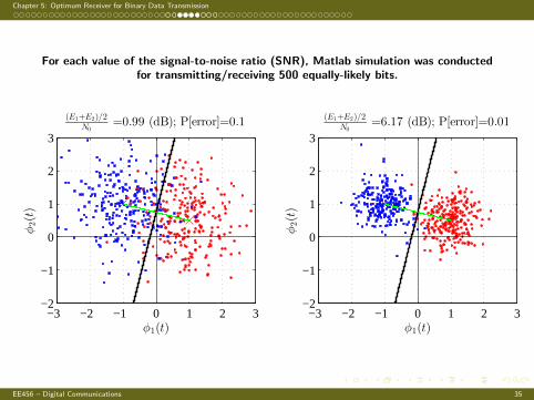
For each value of the signal-to-noise ratio (SNR), Matlab simulation was conductedfor transmitting/receiving 500 equally-likely bits.
−3 −2 −1 0 1 2 3−2
−1
0
1
2
3
(E1+E2)/2N0
=0.99 (dB); P[error]=0.1
φ1(t)
φ2(t)
−3 −2 −1 0 1 2 3−2
−1
0
1
2
3
(E1+E2)/2N0
=6.17 (dB); P[error]=0.01
φ1(t)
φ2(t)
EE456 – Digital Communications 35
Chapter 5: Optimum Receiver for Binary Data Transmission
)(1 tφ
0
)(1 ts
)(2 ts
)(2 tφ
5.0−
5.0
5.0 11−
1
)( Choose 1 ts)( Choose 2 ts
jkl
1r
2r
)(1 tφ
0
)(1 ts
)(2 ts
)(2 tφ
5.0−
5.0
5.0 11−
1
)( Choose 1 ts)( Choose 2 ts
mno
1r
2r
)(1 tφ
0
)(1 ts
)(2 ts
)(2 tφ
5.0−
5.0
5.0 11−
1
)( Choose 1 ts
)( Choose 2 ts
pqr
1r
2r
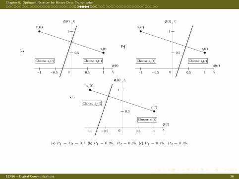
(a) P1 = P2 = 0.5, (b) P1 = 0.25, P2 = 0.75. (c) P1 = 0.75, P2 = 0.25.
EE456 – Digital Communications 36

Chapter 5: Optimum Receiver for Binary Data Transmission
Example 5.7
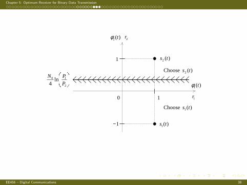
s2(t) = φ1(t) + φ2(t),
s1(t) = φ1(t) − φ2(t).
s
)(1 tφ
0
1
s
)(2 tφ
0 1
1−
1
3
2
1
EE456 – Digital Communications 37
Chapter 5: Optimum Receiver for Binary Data Transmission
)(1 tφ
0
)(1 ts
)(2 ts1
1−
1
)( Choose 2 ts
)( Choose 1 ts
)(2 tφ
ttuv
wwxy
2
10 ln4 P
PN
2r
1r
EE456 – Digital Communications 38
Chapter 5: Optimum Receiver for Binary Data Transmission
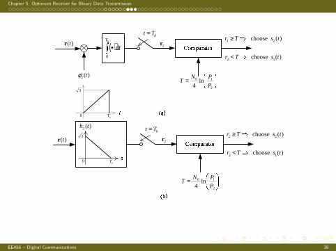
z{|}~�~�{�( )� •bT
t0
d
)(2 tφ
bTt =
����
����
=2
10 ln4 P
PNT
�0bT
3
�~�
)(tr 2r 2 2
2 1
choose ( )
choose ( )
r T s t
r T s t
≥ �
< �
����������bTt =
����
����
=2
10 ln4 P
PNT
)(2 th
�0bT
3
���
2 2
2 1
choose ( )
choose ( )
r T s t
r T s t
≥ �
< �2r)(tr
EE456 – Digital Communications 39
Chapter 5: Optimum Receiver for Binary Data Transmission
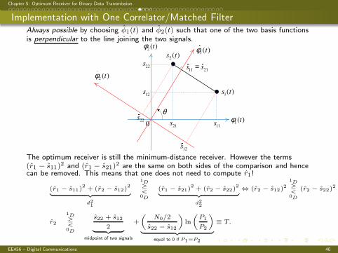
Implementation with One Correlator/Matched FilterAlways possible by choosing φ1(t) and φ2(t) such that one of the two basis functionsis perpendicular to the line joining the two signals.
)(1 tφ
)(1 ts
)(2 ts
)(2 tφ)(1 tφ
θ
)(2 tφ
0 11s
21s
12s
22s
11 21s s=
12s
22s
The optimum receiver is still the minimum-distance receiver. However the terms(r1 − s11)2 and (r1 − s21)2 are the same on both sides of the comparison and hencecan be removed. This means that one does not need to compute r1!
(r1 − s11)2 + (r2 − s12)
2
︸ ︷︷ ︸
d21
1D
R0D
(r1 − s21)2 + (r2 − s22)
2
︸ ︷︷ ︸
d22
⇔ (r2 − s12)2
1D
R0D
(r2 − s22)2
r2
1D
R0D
s22 + s12
2︸ ︷︷ ︸
midpoint of two signals
+
(N0/2
s22 − s12
)
ln
(P1
P2
)
︸ ︷︷ ︸
equal to 0 if P1=P2
≡ T.
EE456 – Digital Communications 40
Chapter 5: Optimum Receiver for Binary Data Transmission
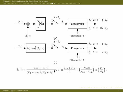
�� ¡¢£¢¤�£( )¥ •bT
t0
d
)(2 tφ
bTt =
T Threshold¦¢§
)(tr 2r 2
2
ˆ 1
ˆ 0
D
D
r T
r T
≥ ¨
< ¨
©ª«¬®¯ª®
bTt =
T Threshold
)(ˆ)( 2 tTth b −= φ
°±²
2r)(tr 2
2
ˆ 1
ˆ 0
D
D
r T
r T
≥ ³
< ³
φ2(t) =s2(t) − s1(t)
(E2 − 2ρ√E1E2 + E1)
12
, T ≡ s22 + s12
2+
(N0/2
s22 − s12
)
ln
(P1
P2
)
.
EE456 – Digital Communications 41
Chapter 5: Optimum Receiver for Binary Data Transmission
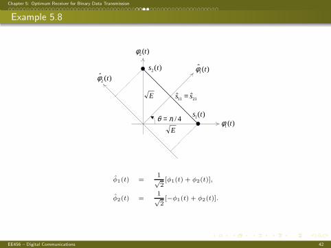
Example 5.8
)(1 tφ)(1 ts
)(2 ts
)(2 tφ
)(1 tφ)(2 tφ
2111 ˆˆ ss =
4/πθ =
E
E
φ1(t) =1√2[φ1(t) + φ2(t)],
φ2(t) =1√2[−φ1(t) + φ2(t)].
EE456 – Digital Communications 42
Chapter 5: Optimum Receiver for Binary Data Transmission
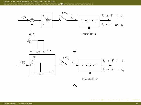
´µ¶·¸¹¸ºµ¹( )» •bT
t0
d
)(2 tφ
bTt =
T Threshold
¼¸½¾0bT
bT
2
2bT
)(tr 2r 2
2
ˆ 1
ˆ 0
D
D
r T
r T
≥ ¿
< ¿
ÀÁÂÃÄÅÄÆÁÅ
bTt =
T Threshold
ÇÈÉ
Ê0
bT
2
2bT
)(th
)(tr 2r 2
2
ˆ 1
ˆ 0
D
D
r T
r T
≥ Ë
< Ë
EE456 – Digital Communications 43
Chapter 5: Optimum Receiver for Binary Data Transmission
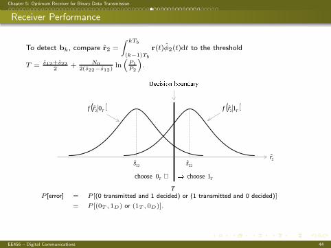
Receiver Performance
To detect bk , compare r2 =
∫ kTb
(k−1)Tb
r(t)φ2(t)dt to the threshold
T = s12+s222
+ N02(s22−s12)
ln(
P1P2
)
.
12s 22s
( )Trf 02 ( )Trf 12
TT 1 choose 0 choose Ì⇐
2r
ÍÎÏÐÑÐÒÓ ÔÒÕÓÖ×ØÙ
TP [error] = P [(0 transmitted and 1 decided) or (1 transmitted and 0 decided)]
= P [(0T , 1D) or (1T , 0D)].
EE456 – Digital Communications 44
Chapter 5: Optimum Receiver for Binary Data Transmission
ÚÛÜÝ Þ
ßàááàâãäßàåæçàèéâêåëìàâíëçàèéâêåëìàâíëîãéïåéâäðññéòàåéâäóôõæöõàä÷ó
ôæøõñéíéáë îãéïåêéñ ùâéøæääôæøõñéíéáë îãéïåêéñ ùâéøæää
óôõæöõàä÷ó
ßàááàâãä ßàåæçàèéâêåë
ìàâíëçàèéâêåëìàâíëîãéïåéâä ðññéòàåéâä
12s 22s
( )Trf 02 ( )Trf 12
TT 1 choose 0 choose ú⇐
2r
ÚÛÜÝ û
T
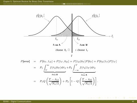
P [error] = P [0T , 1D] + P [1T , 0D ] = P [1D|0T ]P [0T ] + P [0D |1T ]P [1T ]
= P1
∫∞
T
f(r2|0T )dr2
︸ ︷︷ ︸
Area B
+P2
∫ T
−∞
f(r2|1T )dr2
︸ ︷︷ ︸
Area A
= P1Q
(
T − s12√
N0/2
)
+ P2
[
1 − Q
(
T − s22√
N0/2
)]
.
EE456 – Digital Communications 45
Chapter 5: Optimum Receiver for Binary Data Transmission
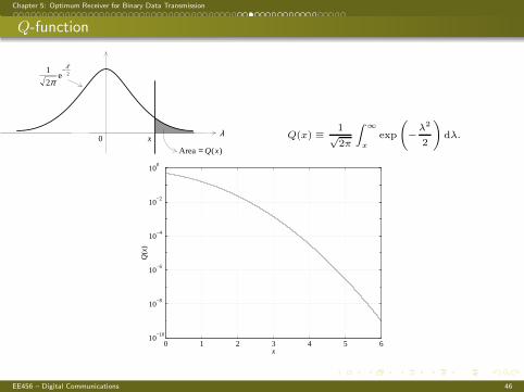
Q-function
üýþÿ������ ������� ��þý��
�üÿý�ÿ ���
� �� ��� � �ý� �����
� ���� �����
� ����������� ����� ����
0λ
x
)(Area xQ=
2
2
e2
1 λ
π−
Q(x) ≡ 1√2π
∫∞
x
exp
(
−λ2
2
)
dλ.
0 1 2 3 4 5 610
−10
10−8
10−6
10−4
10−2
100
x
Q(x
)
EE456 – Digital Communications 46
Chapter 5: Optimum Receiver for Binary Data Transmission
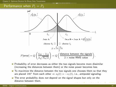
Performance when P1 = P2
12s 22s
( )Trf 02 ( )Trf 12
TT 1choose0choose ⇒⇐
2r
12 22
2
s sT
+=
( )22 12
02 /2
s s
NQ
−=
0
P [error] = Q
(
s22 − s12
2√
N0/2
)
= Q
(distance between the signals
2× noise RMS value
)
.
Probability of error decreases as either the two signals become more dissimilar(increasing the distances between them) or the noise power becomes less.
To maximize the distance between the two signals one chooses them so that theyare placed 180◦ from each other ⇒ s2(t) = −s1(t), i.e., antipodal signaling.
The error probability does not depend on the signal shapes but only on thedistance between them.
EE456 – Digital Communications 47
Chapter 5: Optimum Receiver for Binary Data Transmission
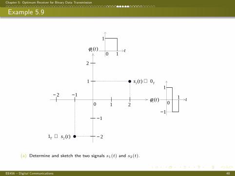
Example 5.9
)(1 tφ
Tts 0)(1 ⇔
)(1 2 tsT ⇔
)(2 tφ
1−
2
2−
1
1−
1
2
2−
0 1
1
t
01
1
t
1−0
(a) Determine and sketch the two signals s1(t) and s2(t).
EE456 – Digital Communications 48
Chapter 5: Optimum Receiver for Binary Data Transmission
(b) The two signals s1(t) and s2(t) are used for the transmission of equally likely bits 0 and 1,respectively, over an additive white Gaussian noise (AWGN) channel. Clearly draw thedecision boundary and the decision regions of the optimum receiver. Write the expression forthe optimum decision rule.
(c) Find and sketch the two orthonormal basis functions φ1(t) and φ2(t) such that the optimumreceiver can be implemented using only the projection r2 of the received signal r(t) onto the
basis function φ2(t). Draw the block diagram of such a receiver that uses a matched filter.
(d) Consider now the following argument put forth by your classmate. She reasons that since the
component of the signals along φ1(t) is not useful at the receiver in determining which bitwas transmitted, one should not even transmit this component of the signal. Thus shemodifies the transmitted signal as follows:
s(M)1 (t) = s1(t) −
(
component of s1(t) along φ1(t))
s(M)2 (t) = s2(t) −
(
component of s2(t) along φ1(t))
Clearly identify the locations of s(M)1 (t) and s
(M)2 (t) in the signal space diagram. What is the
average energy of this signal set? Compare it to the average energy of the original set.Comment.
EE456 – Digital Communications 49

Chapter 5: Optimum Receiver for Binary Data Transmission
0t
3−
)(2 ts
1−
1
)(1 ts
01
3
t
1−
EE456 – Digital Communications 50

Chapter 5: Optimum Receiver for Binary Data Transmission
)(1 tφ
Tts 0)(1 ⇔
)(1 2 tsT ⇔
)(2 tφ
1−
2
2−
1
1−
1
2
2−
0
2( )tφ
4
πθ = −
�������� ���� !"# D0
D1
1( )tφ
2 ( )Ms t
1 ( )Ms t
01
1
t
1−
0 1
1
t
EE456 – Digital Communications 51
Chapter 5: Optimum Receiver for Binary Data Transmission
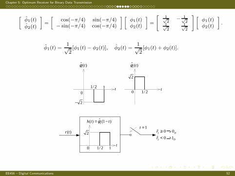
[φ1(t)
φ2(t)
]
=
[cos(−π/4) sin(−π/4)
− sin(−π/4) cos(−π/4)
] [φ1(t)φ2(t)
]
=
[1√2
− 1√2
1√2
1√2
] [φ1(t)φ2(t)
]
.
φ1(t) =1√2[φ1(t) − φ2(t)], φ2(t) =
1√2[φ1(t) + φ2(t)].
0t
01 t
2−
1/ 2
2
1/ 2
1( )tφ 2( )tφ
2( ) (1 )h t tφ= −1t =
2
2
ˆ 0 0
ˆ 0 1D
D
r
r
≥ $
< $
)(tr
0t
2
1/ 2 1
EE456 – Digital Communications 52
Chapter 5: Optimum Receiver for Binary Data Transmission
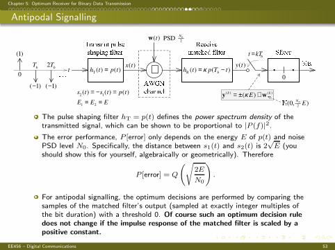
Antipodal Signalling
bkTt =
+
( )tw
( ) ( )( )
k kEκ= ± +y w
( )x tt
0
(1)
( 1)− ( 1)−
bT 2
bT ( )y t
T ( ) ( )h t p t= R ( ) ( )bh t p T tκ= −
0
2PSD
N
0
0
2(0, )
NE
2 1
1 2
( ) ( ) ( )s t s t p t
E E E
= − == =
The pulse shaping filter hT = p(t) defines the power spectrum density of thetransmitted signal, which can be shown to be proportional to |P (f)|2.The error performance, P [error] only depends on the energy E of p(t) and noisePSD level N0. Specifically, the distance between s1(t) and s2(t) is 2
√E (you
should show this for yourself, algebraically or geometrically). Therefore
P [error] = Q
(√
2E
N0
)
.
For antipodal signalling, the optimum decisions are performed by comparing thesamples of the matched filter’s output (sampled at exactly integer multiples ofthe bit duration) with a threshold 0. Of course such an optimum decision ruledoes not change if the impulse response of the matched filter is scaled by apositive constant.
EE456 – Digital Communications 53
Chapter 5: Optimum Receiver for Binary Data Transmission
Scaling the matched filter’s impulse response hR(t) does not change the receiverperformance because it scales both signal and noise components by the samefactor, leaving the signal-to-noise ratio (SNR) of the decision variable unchanged!
In the above block diagram, hR(t) = κp(Tb − t). We have been using κ = 1/√E
in order to represent the signals on the signal space diagram (which would be at±√E) and to conclude that the variance of the noise component is exactly N0/2.
For an arbitrary scaling factor κ, the signal component becomes ±κE, while thevariance of the noise component is N0
2κ2E. Thus, the SNR is
SNR =Signal power
Noise power=
(±κE)2
N02κ2E
=2E
N0, (indepedent of κ!)
In terms of the SNR, the error performance of antipodal signalling is
P [error] = Q
(√
2E
N0
)
= Q(√
SNR)
In fact, it can be proved that the receive filter that maximizes the SNR of thedecision variable must be the matched filter. It is important to emphasize thatthe matching property here concerns the shapes of the impulse responses of thetransmit and receive filters.
EE456 – Digital Communications 54
Chapter 5: Optimum Receiver for Binary Data Transmission
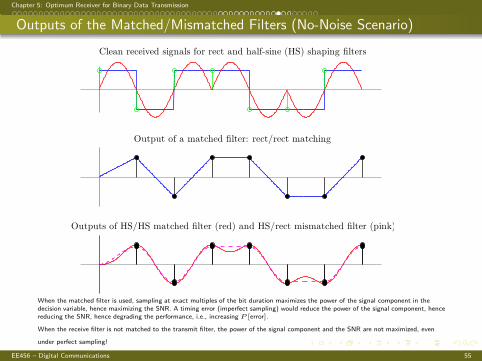
Outputs of the Matched/Mismatched Filters (No-Noise Scenario)
Clean received signals for rect and half-sine (HS) shaping filters
Output of a matched filter: rect/rect matching
Outputs of HS/HS matched filter (red) and HS/rect mismatched filter (pink)
When the matched filter is used, sampling at exact multiples of the bit duration maximizes the power of the signal component in thedecision variable, hence maximizing the SNR. A timing error (imperfect sampling) would reduce the power of the signal component, hencereducing the SNR, hence degrading the performance, i.e., increasing P [error].
When the receive filter is not matched to the transmit filter, the power of the signal component and the SNR are not maximized, even
under perfect sampling!
EE456 – Digital Communications 55
Chapter 5: Optimum Receiver for Binary Data Transmission
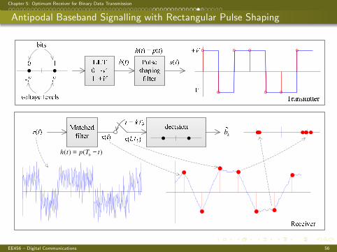
Antipodal Baseband Signalling with Rectangular Pulse Shaping
kb
( ) ( )b
h t p T t= −
EE456 – Digital Communications 56
Chapter 5: Optimum Receiver for Binary Data Transmission
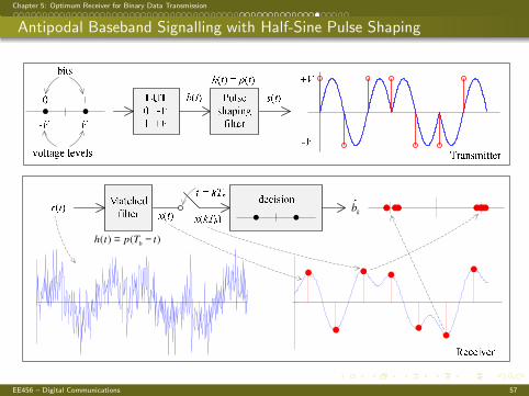
Antipodal Baseband Signalling with Half-Sine Pulse Shaping
kb
( ) ( )b
h t p T t= −
EE456 – Digital Communications 57
Chapter 5: Optimum Receiver for Binary Data Transmission
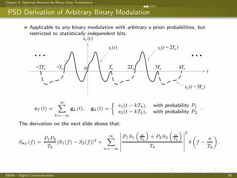
PSD Derivation of Arbitrary Binary Modulation
Applicable to any binary modulation with arbitrary a priori probabilities, butrestricted to statistically independent bits.
t0
( )T
s t
bT 2
bT 4
bT
1( )s t
1( 2 )
bs t T−
bT−2
bT− 3
bT
2( 3 )
bs t T−
sT (t) =∞∑
k=−∞gk(t), gk(t) =
{s1(t − kTb), with probability P1
s2(t − kTb), with probability P2.
The derivation on the next slide shows that:
SsT (f) =P1P2
Tb
|S1(f)− S2(f)|2 +∞∑
n=−∞
∣∣∣∣∣∣
P1S1
(nTb
)
+ P2S2
(nTb
)
Tb
∣∣∣∣∣∣
2
δ
(
f − n
Tb
)
.
EE456 – Digital Communications 58
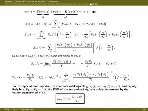
Chapter 5: Optimum Receiver for Binary Data Transmission
sT (t) = E{sT (t)}︸ ︷︷ ︸
DC
+ sT (t) − E{sT (t)}︸ ︷︷ ︸
AC
= v(t) + q(t)
v(t) = E{sT (t)} =∞∑
k=−∞
[P1s1(t − kTb) + P2s2(t − kTb)]
Sv(f) =
∞∑
n=−∞
|Dn|2δ(
f − n
Tb
)
, Dn =1
Tb
[
P1S1
(n
Tb
)
+ P2S2
(n
Tb
)]
,
Sv(f) =∞∑
n=−∞
∣∣∣∣∣∣
P1S1
(nTb
)
+ P2S2
(nTb
)
Tb
∣∣∣∣∣∣
2
δ
(
f − n
Tb
)
.
To calculate Sq(f), apply the basic definition of PSD:
Sq(f) = limT→∞
E{|GT (f)|2}T
= · · · = P1P2
Tb
|S1(f) − S2(f)|2.
SsT(f) =
P1P2
Tb
|S1(f) − S2(f)|2 +
∞∑
n=−∞
∣∣∣∣∣∣
P1S1
(nTb
)
+ P2S2
(nTb
)
Tb
∣∣∣∣∣∣
2
δ
(
f − n
Tb
)
.
For the special, but important case of antipodal signalling, s2(t) = −s1(t) = p(t), and equallylikely bits, P1 = P2 = 0.5, the PSD of the transmitted signal is solely determined by theFourier transform of p(t):
SsT(f) =
|P (f)|2
Tb
EE456 – Digital Communications 59
Chapter 5: Optimum Receiver for Binary Data Transmission
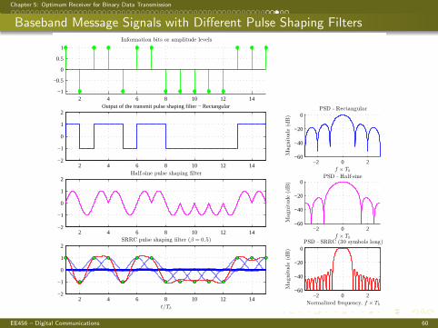
Baseband Message Signals with Different Pulse Shaping Filters
2 4 6 8 10 12 14−1
−0.5
0
0.5
1
Information bits or amplitude levels
2 4 6 8 10 12 14−2
−1
0
1
2Output of the transmit pulse shaping filter − Rectangular
−2 0 2−60
−40
−20
0
f × Tb
Magnitude(dB)
PSD - Rectangular
2 4 6 8 10 12 14−2
−1
0
1
2Half-sine pulse shaping filter
−2 0 2−60
−40
−20
0
f × Tb
Magnitude(dB)
PSD - Half-sine
2 4 6 8 10 12 14−2
−1
0
1
2
t/Tb
SRRC pulse shaping filter (β = 0.5)
−2 0 2−60
−40
−20
0
Normalized frequency, f × Tb
Magnitude(dB)
PSD - SRRC (30 symbols long)
EE456 – Digital Communications 60
Chapter 5: Optimum Receiver for Binary Data Transmission
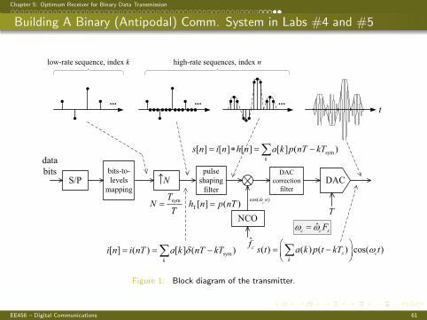
Building A Binary (Antipodal) Comm. System in Labs #4 and #5
S/Pbits-to-
levels
mapping
pulse
shaping
filter
t
DACN
data
bits
NCO
ˆcf
ˆcos( )cnw
T[ ] ( )h n p nT=symTN
T=
T
sym[ ] ( ) [ ] ( )k
i n i nT a k nT kTd= = -å
sym[ ] [ ] [ ] [ ] ( )k
s n i n h n a k p nT kT= * = -å
( ) ( ) ( ) cos( )s c
k
s t a k p t kT twæ ö
= -ç ÷è øå
low-rate sequence, index k high-rate sequences, index n
...... ...
DAC
correction
filter
ˆc c sFw w=
Figure 1: Block diagram of the transmitter.
EE456 – Digital Communications 61
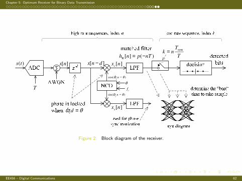
Chapter 5: Optimum Receiver for Binary Data Transmission
∑
cos( )cnω θ−
sin( )cnω θ−
cf
[ ]c
x n
[ ]s
x n
[ ]x n [ ]x n d−
cdω θ=
R[ ] ( )h n p nT= −
T
symTk n
T=
( )s t
θ
Figure 2: Block diagram of the receiver.
EE456 – Digital Communications 62