Embed Size (px)
Citation preview
EE290T: Advanced Reconstruction Methods for MagneticResonance Imaging
Martin Uecker
Introduction
Topics:
I Image Reconstruction as Inverse Problem
I Parallel Imaging
I Non-Cartestian MRI
I Subspace Methods
I Model-based Reconstruction
I Compressed Sensing
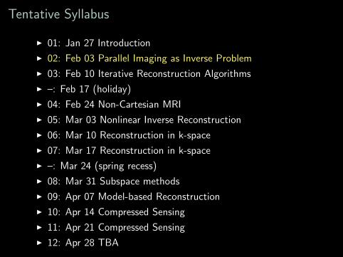
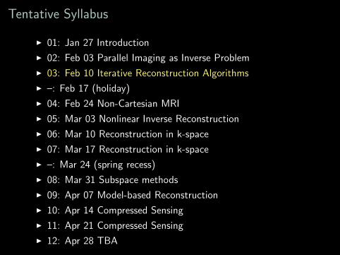
Tentative Syllabus
I 01: Jan 27 Introduction
I 02: Feb 03 Parallel Imaging as Inverse Problem
I 03: Feb 10 Iterative Reconstruction Algorithms
I –: Feb 17 (holiday)
I 04: Feb 24 Non-Cartesian MRI
I 05: Mar 03 Nonlinear Inverse Reconstruction
I 06: Mar 10 Reconstruction in k-space
I 07: Mar 17 Reconstruction in k-space
I –: Mar 24 (spring recess)
I 08: Mar 31 Subspace methods
I 09: Apr 07 Model-based Reconstruction
I 10: Apr 14 Compressed Sensing
I 11: Apr 21 Compressed Sensing
I 12: Apr 28 TBA
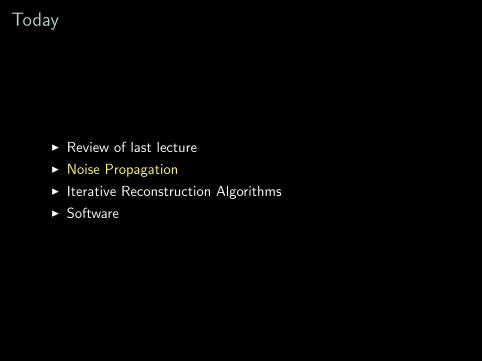
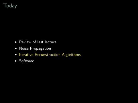
Today
I Review of last lecture
I Noise Propagation
I Iterative Reconstruction Algorithms
I Software
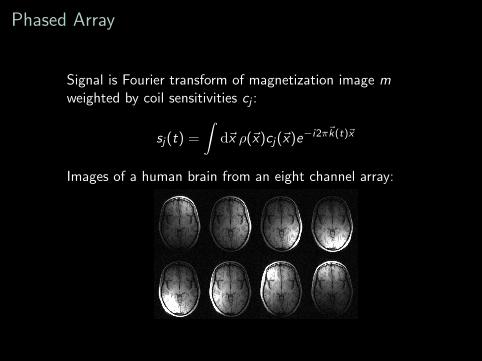
Phased Array
Signal is Fourier transform of magnetization image mweighted by coil sensitivities cj :
sj(t) =
∫d~x ρ(~x)cj(~x)e−i2π~k(t)~x
Images of a human brain from an eight channel array:
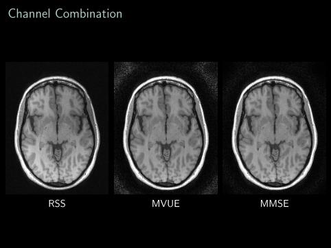
Channel Combination
RSS MVUE MMSE
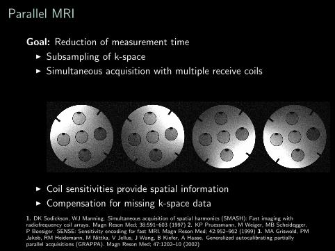
Parallel MRI
Goal: Reduction of measurement time
I Subsampling of k-space
I Simultaneous acquisition with multiple receive coils
I Coil sensitivities provide spatial information
I Compensation for missing k-space data
1. DK Sodickson, WJ Manning. Simultaneous acquisition of spatial harmonics (SMASH): Fast imaging withradiofrequency coil arrays. Magn Reson Med; 38:591–603 (1997) 2. KP Pruessmann, M Weiger, MB Scheidegger,P Boesiger. SENSE: Sensitivity encoding for fast MRI. Magn Reson Med; 42:952–962 (1999) 3. MA Griswold, PMJakob, RM Heidemann, M Nittka, V Jellus, J Wang, B Kiefer, A Haase. Generalized autocalibrating partiallyparallel acquisitions (GRAPPA). Magn Reson Med; 47:1202–10 (2002)
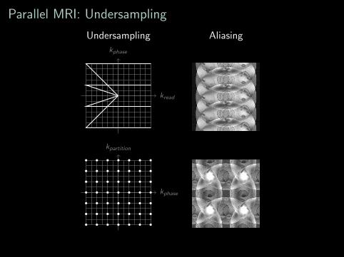
Parallel MRI: Undersampling
Undersampling Aliasing
kread
kphase
kphase
kpartition
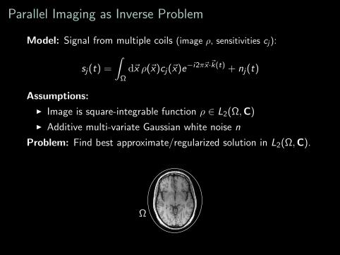
Parallel Imaging as Inverse Problem
Model: Signal from multiple coils (image ρ, sensitivities cj):
sj(t) =
∫Ωd~x ρ(~x)cj(~x)e−i2π~x ·~k(t) + nj(t)
Assumptions:
I Image is square-integrable function ρ ∈ L2(Ω,C)
I Additive multi-variate Gaussian white noise n
Problem: Find best approximate/regularized solution in L2(Ω,C).
Ω
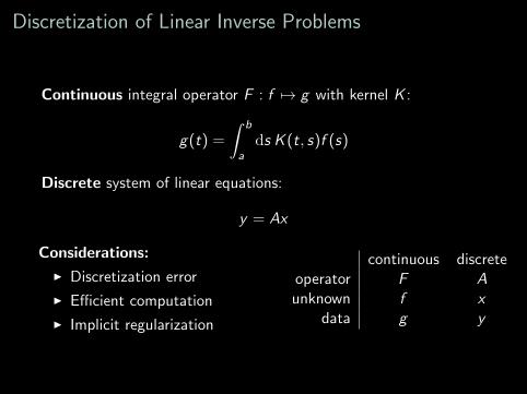
Discretization of Linear Inverse Problems
Continuous integral operator F : f 7→ g with kernel K :
g(t) =
∫ b
ads K (t, s)f (s)
Discrete system of linear equations:
y = Ax
Considerations:
I Discretization error
I Efficient computation
I Implicit regularization
continuous discreteoperator F Aunknown f x
data g y
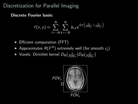
Discretization for Parallel Imaging
Discrete Fourier basis:
f (x , y) ≈N∑
l=−N
N∑k=−N
al ,kei2π
(kx
FOVy+ ly
FOVy
)
I Efficient computation (FFT)
I Approximates R(FH) extremely well (for smooth cj)
I Voxels: Dirichlet kernel DN( xFOVx
)DN( yFOVy
)
Ω
FOVx
FOVy
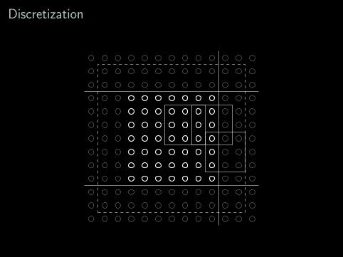
Discretization
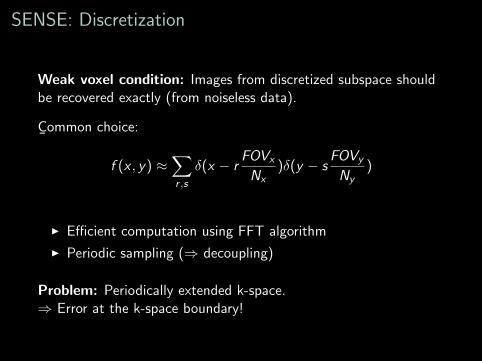
SENSE: Discretization
Weak voxel condition: Images from discretized subspace shouldbe recovered exactly (from noiseless data).
C¯
ommon choice:
f (x , y) ≈∑r ,s
δ(x − rFOVx
Nx)δ(y − s
FOVy
Ny)
I Efficient computation using FFT algorithm
I Periodic sampling (⇒ decoupling)
Problem: Periodically extended k-space.⇒ Error at the k-space boundary!
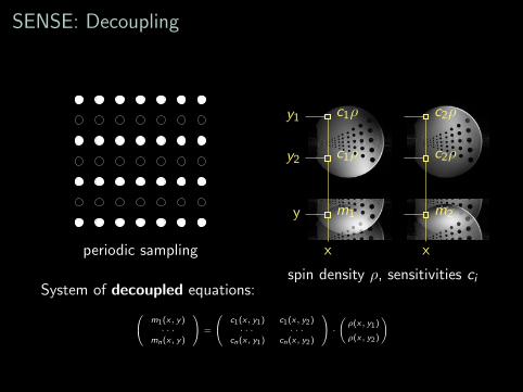
SENSE: Decoupling
periodic sampling
m2m1
c2ρc1ρ
c2ρc1ρ
x
y
x
y1
y2
spin density ρ, sensitivities ciSystem of decoupled equations:
m1(x, y)· · ·
mn(x, y)
=
c1(x, y1) c1(x, y2)· · · · · ·
cn(x, y1) cn(x, y2)
· ( ρ(x, y1)
ρ(x, y2)
)
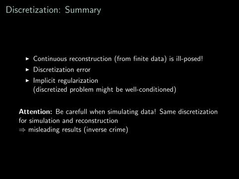
Discretization: Summary
I Continuous reconstruction (from finite data) is ill-posed!
I Discretization error
I Implicit regularization(discretized problem might be well-conditioned)
Attention: Be carefull when simulating data! Same discretizationfor simulation and reconstruction⇒ misleading results (inverse crime)
Today
I Review of last lecture
I Noise Propagation
I Iterative Reconstruction Algorithms
I Software
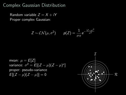
Complex Gaussian Distribution
Random variable Z = X + iYProper complex Gaussian:
Z ∼ CN (µ, σ2) p(Z ) =1
σπe−|Z−µ|2
σ2
mean: µ = E [Z ]variance: σ2 = E [(Z − µ)(Z − µ)?]proper: pseudo-varianceE [(Z − µ)(Z − µ)] = 0 R
I
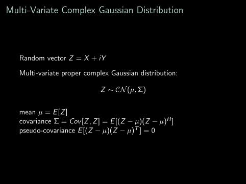
Multi-Variate Complex Gaussian Distribution
Random vector Z = X + iY
Multi-variate proper complex Gaussian distribution:
Z ∼ CN (µ,Σ)
mean µ = E [Z ]covariance Σ = Cov [Z ,Z ] = E [(Z − µ)(Z − µ)H ]pseudo-covariance E [(Z − µ)(Z − µ)T ] = 0
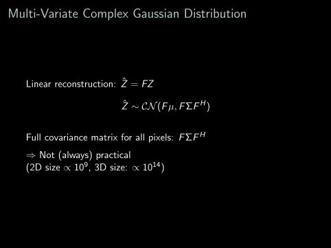
Multi-Variate Complex Gaussian Distribution
Linear reconstruction: Z = FZ
Z ∼ CN (Fµ,FΣFH)
Full covariance matrix for all pixels: FΣFH
⇒ Not (always) practical(2D size ∝ 109, 3D size: ∝ 1014)
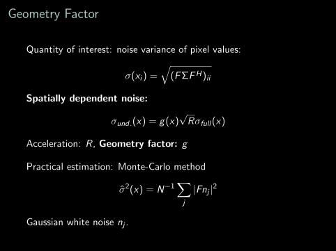
Geometry Factor
Quantity of interest: noise variance of pixel values:
σ(xi ) =√
(FΣFH)ii
Spatially dependent noise:
σund .(x) = g(x)√Rσfull(x)
Acceleration: R, Geometry factor: g
Practical estimation: Monte-Carlo method
σ2(x) = N−1∑j
|Fnj |2
Gaussian white noise nj .
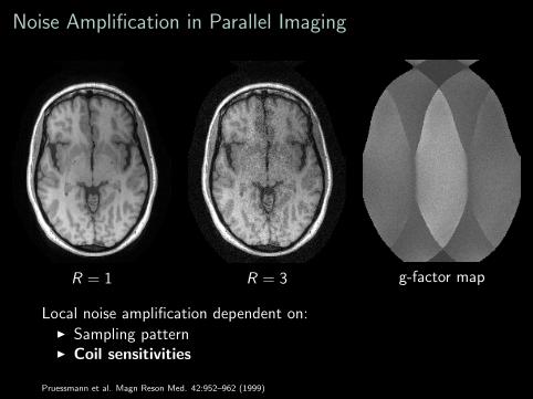
Noise Amplification in Parallel Imaging
R = 1 R = 3 g-factor map
Local noise amplification dependent on:I Sampling patternI Coil sensitivities
Pruessmann et al. Magn Reson Med. 42:952–962 (1999)
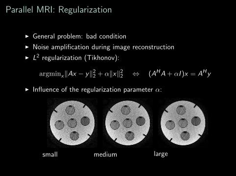
Parallel MRI: Regularization
I General problem: bad condition
I Noise amplification during image reconstruction
I L2 regularization (Tikhonov):
argminx‖Ax − y‖22 + α‖x‖2
2 ⇔ (AHA + αI )x = AHy
I Influence of the regularization parameter α:
small medium large
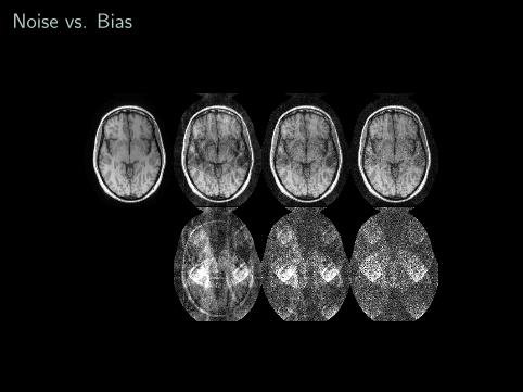
Noise vs. Bias
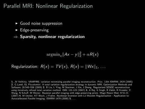
Parallel MRI: Nonlinear Regularization
I Good noise suppression
I Edge-preserving
⇒ Sparsity, nonlinear regularization
argminx‖Ax − y‖22 + αR(x)
Regularization: R(x) = TV (x), R(x) = ‖Wx‖1, . . .
1. JV Velikina. VAMPIRE: variation minimizing parallel imaging reconstruction. Proc. 13th ISMRM; 2424 (2005)2. G Landi, EL Piccolomini. A total variation regularization strategy in dynamic MRI, Optimization Methods andSoftware; 20:545–558 (2005) 2. B Liu, L Ying, M Steckner, J Xie, J Sheng. Regularized SENSE reconstructionusing iteratively refined total variation method. ISBI; 121-123 (2007) 3. A Raj, G Singh, R Zabih, B Kressler, YWang, N Schuff, M Weiner. Bayesian parallel imaging with edge-preserving priors. Magn Reson Med; 57:8–21(2007) 4. M Uecker, KT Block, J Frahm. Nonlinear Inversion with L1-Wavelet Regularization - Application toAutocalibrated Parallel Imaging. ISMRM 1479 (2008) 5. . . .
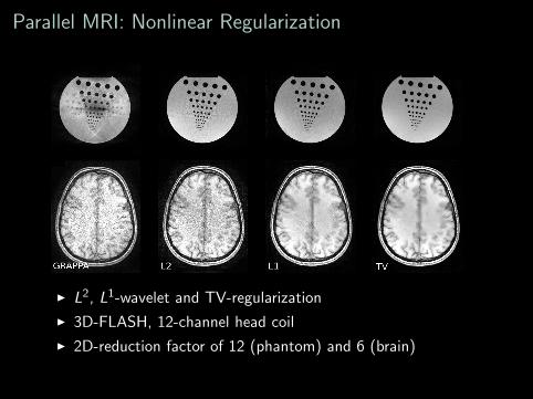
Parallel MRI: Nonlinear Regularization
I L2, L1-wavelet and TV-regularization
I 3D-FLASH, 12-channel head coil
I 2D-reduction factor of 12 (phantom) and 6 (brain)
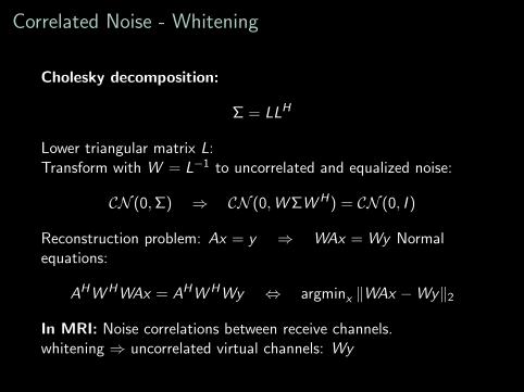
Correlated Noise - Whitening
Cholesky decomposition:
Σ = LLH
Lower triangular matrix L:Transform with W = L−1 to uncorrelated and equalized noise:
CN (0,Σ) ⇒ CN (0,WΣWH) = CN (0, I )
Reconstruction problem: Ax = y ⇒ WAx = Wy Normalequations:
AHWHWAx = AHWHWy ⇔ argminx ‖WAx −Wy‖2
In MRI: Noise correlations between receive channels.whitening ⇒ uncorrelated virtual channels: Wy
Today
I Review of last lecture
I Noise Propagation
I Iterative Reconstruction Algorithms
I Software
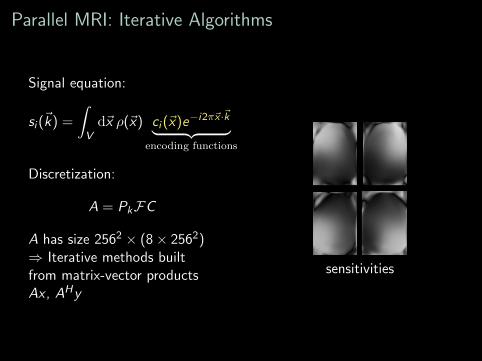
Parallel MRI: Iterative Algorithms
Signal equation:
si (~k) =
∫Vd~x ρ(~x) ci (~x)e−i2π~x ·~k︸ ︷︷ ︸
encoding functions
Discretization:
A = PkFC
A has size 2562 × (8× 2562)⇒ Iterative methods builtfrom matrix-vector productsAx , AHy
sensitivities
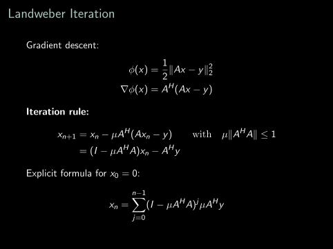
Landweber Iteration
Gradient descent:
φ(x) =1
2‖Ax − y‖2
2
∇φ(x) = AH(Ax − y)
Iteration rule:
xn+1 = xn − µAH(Axn − y) with µ‖AHA‖ ≤ 1
= (I − µAHA)xn − AHy
Explicit formula for x0 = 0:
xn =n−1∑j=0
(I − µAHA)jµAHy
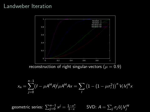
Landweber Iteration
0
0.2
0.4
0.6
0.8
1
0 0.2 0.4 0.6 0.8 1
iteration 1iteration 2
iteration 10iteration 50
reconstruction of right singular-vectors (µ = 0.9)
xn =n−1∑j=0
(I − µAHA)jµAHAx =∑l
(1− (1− µσ2
l ))n
VlVHl x
geometric series:∑n−1
j=0 x j = 1−xn
1−x SVD: A =∑
j σjUjVHj
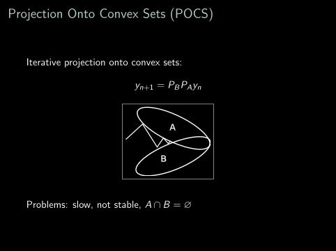
Projection Onto Convex Sets (POCS)
Iterative projection onto convex sets:
yn+1 = PBPAyn
A
B
Problems: slow, not stable, A ∩ B = ∅
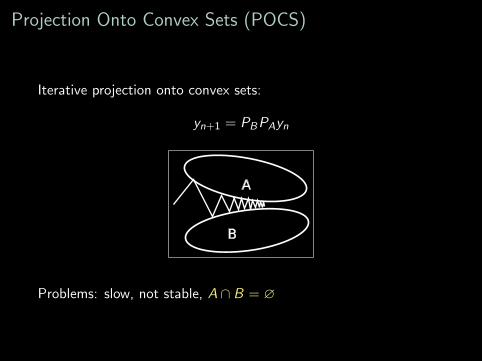
Projection Onto Convex Sets (POCS)
Iterative projection onto convex sets:
yn+1 = PBPAyn
A
B
Problems: slow, not stable, A ∩ B = ∅
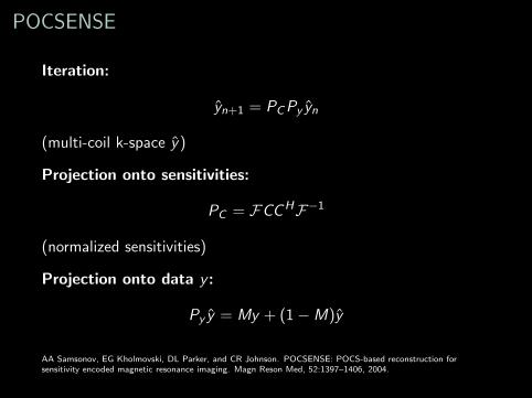
POCSENSE
Iteration:
yn+1 = PCPy yn
(multi-coil k-space y)
Projection onto sensitivities:
PC = FCCHF−1
(normalized sensitivities)
Projection onto data y :
Py y = My + (1−M)y
AA Samsonov, EG Kholmovski, DL Parker, and CR Johnson. POCSENSE: POCS-based reconstruction forsensitivity encoded magnetic resonance imaging. Magn Reson Med, 52:1397–1406, 2004.
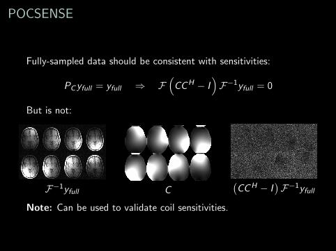
POCSENSE
Fully-sampled data should be consistent with sensitivities:
PCyfull = yfull ⇒ F(CCH − I
)F−1yfull = 0
But is not:
F−1yfull C(CCH − I
)F−1yfull
Note: Can be used to validate coil sensitivities.
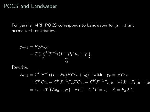
POCS and Landweber
For parallel MRI: POCS corresponds to Landweber for µ = 1 andnormalized sensitivities.
yn+1 = PCPyyn
= FC CHF−1((I − Pk)yn + y0)︸ ︷︷ ︸xn
Rewrite:
xn+1 = CHF−1((I − Pk)FCxn + y0) with yn = FCxn= CHCxn − CHF−1PkFCxn + CHF−1Pky0 with Pky0 = y0
= xn − AH(Axn − y0) with CHC = I , A = PkFC
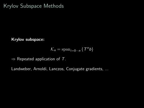
Krylov Subspace Methods
Krylov subspace:
Kn = spani=0···n T nb
⇒ Repeated application of T .
Landweber, Arnoldi, Lanczos, Conjugate gradients, ...

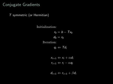
Conjugate Gradients
T symmetric (or Hermitian)
Initialization:
r0 = b − Tx0
d0 = r0
Iteration:
qi ⇐ Tdi
α =|ri |2
R rHi qi
xi+1 ⇐ xi + αdi
ri+1 ⇐ ri − αqi
β =|ri+1|2
|ri |2
di+1 ⇐ ri+1 + βdi
Conjugate Gradients
T symmetric (or Hermitian)
Initialization:
r0 = b − Tx0
d0 = r0
Iteration:
qi ⇐ Tdi
xi+1 ⇐ xi + αdi
ri+1 ⇐ ri − αqi
di+1 ⇐ ri+1 + βdi
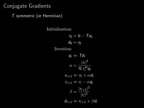
Conjugate Gradients
T symmetric (or Hermitian)
Initialization:
r0 = b − Tx0
d0 = r0
Iteration:
qi ⇐ Tdi
α =|ri |2
R rHi qi
xi+1 ⇐ xi + αdi
ri+1 ⇐ ri − αqi
β =|ri+1|2
|ri |2
di+1 ⇐ ri+1 + βdi
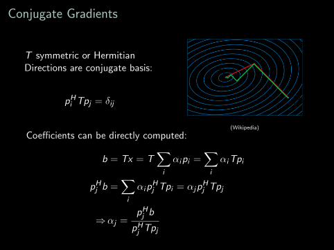
Conjugate Gradients
T symmetric or HermitianDirections are conjugate basis:
pHi Tpj = δij
(Wikipedia)
Coefficients can be directly computed:
b = Tx = T∑i
αipi =∑i
αiTpi
pHj b =∑i
αipHj Tpi = αjp
Hj Tpj
⇒αj =pHj b
pHj Tpj
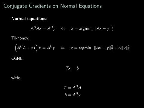
Conjugate Gradients on Normal Equations
Normal equations:
AHAx = AHy ⇔ x = argminx ‖Ax − y‖22
Tikhonov:(AHA + αI
)x = AHy ⇔ x = argminx ‖Ax − y‖2
2 + α‖x‖22
CGNE:
Tx = b
with:
T = AHA
b = AHy
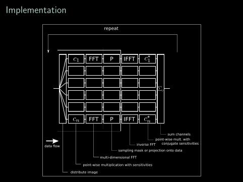
Implementation
FFT IFFTP
FFT IFFTP
distribute image
point-wise multiplication with sensitivities
multi-dimensional FFT
sampling mask or projection onto data
inverse FFT
point-wise mult. with conjugate sensitivities
sum channels
repeat
data flow

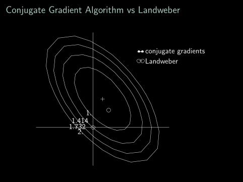
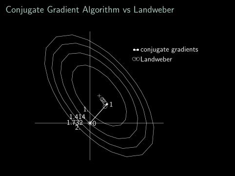
Conjugate Gradient Algorithm vs Landweber
conjugate gradients
Landweber
1.1.414
1.7322.

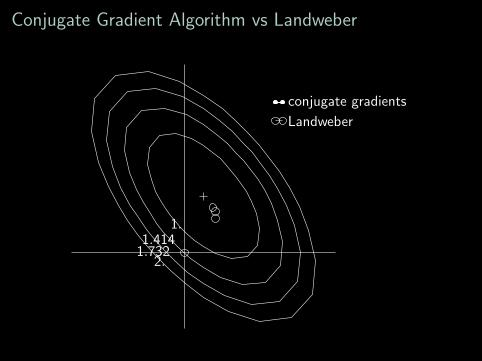
Conjugate Gradient Algorithm vs Landweber
conjugate gradients
Landweber
1.1.414
1.7322.
Conjugate Gradient Algorithm vs Landweber
conjugate gradients
Landweber
1.1.414
1.7322.

Conjugate Gradient Algorithm vs Landweber
conjugate gradients
Landweber
1.1.414
1.7322.
Conjugate Gradient Algorithm vs Landweber
conjugate gradients
Landweber
1.1.414
1.7322.

Conjugate Gradient Algorithm vs Landweber
conjugate gradients
Landweber
1.1.414
1.7322.

Conjugate Gradient Algorithm vs Landweber
conjugate gradients
Landweber
1.1.414
1.7322.
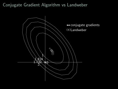
Conjugate Gradient Algorithm vs Landweber
conjugate gradients
Landweber
0
1.1.414
1.7322.
Conjugate Gradient Algorithm vs Landweber
conjugate gradients
Landweber
0
11.
1.4141.732
2.
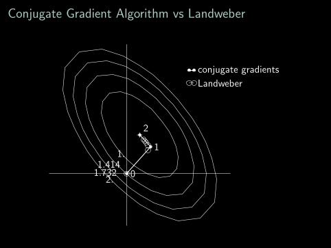
Conjugate Gradient Algorithm vs Landweber
conjugate gradients
Landweber
0
1
2
1.1.414
1.7322.
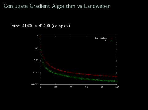
Conjugate Gradient Algorithm vs Landweber
Size: 41400× 41400 (complex)
0.0001
0.001
0.01
0.1
1
0 20 40 60 80 100
LandweberCG
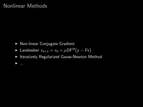
Nonlinear Methods
I Non-linear Conjugate Gradient
I Landweber xn+1 = xn + µDFH(y − Fx)
I Iteratively Regularized Gauss-Newton Method
I ...
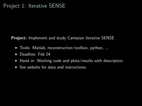
Project 1: Iterative SENSE
Project: Implement and study Cartesian iterative SENSE
I Tools: Matlab, reconstruction toolbox, python, ...
I Deadline: Feb 24
I Hand in: Working code and plots/results with description.
I See website for data and instructions.
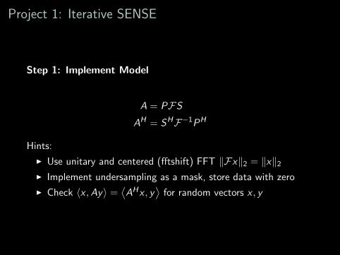
Project 1: Iterative SENSE
Step 1: Implement Model
A = PFSAH = SHF−1PH
Hints:
I Use unitary and centered (fftshift) FFT ‖Fx‖2 = ‖x‖2
I Implement undersampling as a mask, store data with zero
I Check 〈x ,Ay〉 =⟨AHx , y
⟩for random vectors x , y
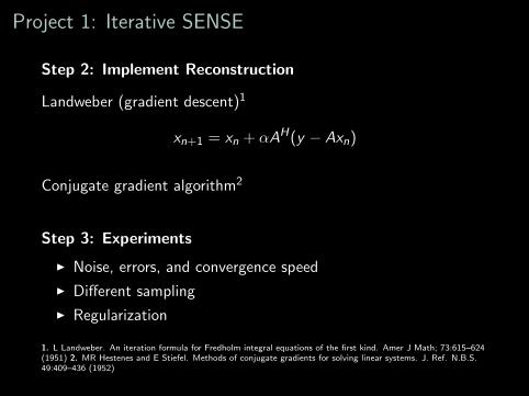
Project 1: Iterative SENSE
Step 2: Implement Reconstruction
Landweber (gradient descent)1
xn+1 = xn + αAH(y − Axn)
Conjugate gradient algorithm2
Step 3: Experiments
I Noise, errors, and convergence speed
I Different sampling
I Regularization
1. L Landweber. An iteration formula for Fredholm integral equations of the first kind. Amer J Math; 73:615–624(1951) 2. MR Hestenes and E Stiefel. Methods of conjugate gradients for solving linear systems. J. Ref. N.B.S.49:409–436 (1952)
Today
I Review of last lecture
I Noise Propagation
I Iterative Reconstruction Algorithms
I Software
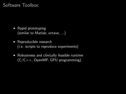
Software Toolbox
I Rapid prototyping(similar to Matlab, octave, ...)
I Reproducible research(i.e. scripts to reproduce experiments)
I Robustness and clinically feasible runtime(C/C++, OpenMP, GPU programming)
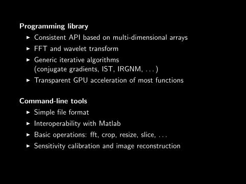
Programming library
I Consistent API based on multi-dimensional arrays
I FFT and wavelet transform
I Generic iterative algorithms(conjugate gradients, IST, IRGNM, . . . )
I Transparent GPU acceleration of most functions
Command-line tools
I Simple file format
I Interoperability with Matlab
I Basic operations: fft, crop, resize, slice, . . .
I Sensitivity calibration and image reconstruction
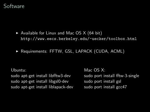
Software
I Available for Linux and Mac OS X (64 bit)http://www.eecs.berkeley.edu/~uecker/toolbox.html
I Requirements: FFTW, GSL, LAPACK (CUDA, ACML)
Ubuntu:sudo apt-get install libfftw3-devsudo apt-get install libgsl0-devsudo apt-get install liblapack-dev
Mac OS X:sudo port install fftw-3-singlesudo port install gslsudo port install gcc47
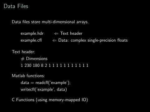
Data Files
Data files store multi-dimensional arrays.
example.hdr ⇐ Text header
example.cfl ⇐ Data: complex single-precision floats
Text header:
# Dimensions
1 230 180 8 2 1 1 1 1 1 1 1 1 1 1 1
Matlab functions:
data = readcfl(’example’);
writecfl(’example’, data)
C Functions (using memory-mapped IO)
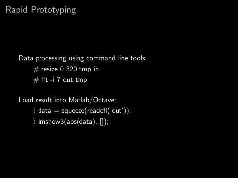
Rapid Prototyping
Data processing using command line tools:
# resize 0 320 tmp in
# fft -i 7 out tmp
Load result into Matlab/Octave:
〉 data = squeeze(readcfl(’out’));
〉 imshow3(abs(data), []);
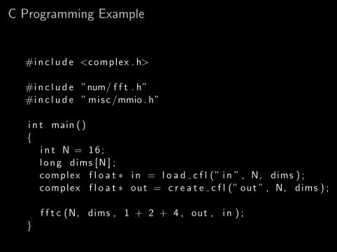
C Programming Example
#i n c l u d e <complex . h>
#i n c l u d e ”num/ f f t . h”#i n c l u d e ” misc /mmio . h”
i n t main ( )
i n t N = 1 6 ;l o n g dims [N ] ;complex f l o a t ∗ i n = l o a d c f l (” i n ” , N, dims ) ;complex f l o a t ∗ out = c r e a t e c f l (” out ” , N, dims ) ;
f f t c (N, dims , 1 + 2 + 4 , out , i n ) ;
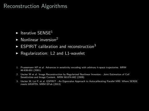
Reconstruction Algorithms
I Iterative SENSE1
I Nonlinear inversion2
I ESPIRiT calibration and reconstruction3
I Regularization: L2 and L1-wavelet
1. Pruessmann KP et al. Advances in sensitivity encoding with arbitrary k-space trajectories. MRM46:638-651 (2001)
2. Uecker M et al. Image Reconstruction by Regularized Nonlinear Inversion - Joint Estimation of CoilSensitivities and Image Content. MRM 60:674-682 (2008)
3. Uecker M, Lai P, et al. ESPIRiT - An Eigenvalue Approach to Autocalibrating Parallel MRI: Where SENSEmeets GRAPPA. MRM EPub (2013)