EE264 Project : Simultaneous Structure and TextureImage Inpainting

Shane BrennanEE 264 - Spring 2007shanerb@soe.ucsc.edu

June 6, 2007

Abstract

Image inpainting is an old technique for filling in missing or damaged regions of an image.The general problem is: given an image and a user-defined region of the image to be filled, fillthe region in such a manner that one cannot tell that the region has been altered. In this projectI have implemented the method proposed by Bertalmio et al in their 2003 paper “Simultane-ous Structure and Texture Image Inpainting” to accomplish this task automatically on digitalimages.

1 Traditional Image InpaintingImage inpainting is a method of modifying images in such a manner that one cannot detect themodification to the image. A typical application of inpainting is the restoration of old and decay-ing paintings. In this scenario, cracks or other defects have appeared in the work and one wishesto restore the piece so that there are no visible defects. An example of such restoration can beseen in Figure 1. To perform this restoration one has to paint over the cracks in order to hide theirexistence. If a photograph or some other copy of the original, undamaged artwork exists that canbe used as a reference it is a relatively straightforward, if not tedious, task to painstakingly recreatethe original image by using the reference image. However, it is often the case that a referenceimage is unavailable. In this case it is up to the restorator to fill in the damaged regions on theirown. A common approach for accomplishing this inpainting task is to fill in the damaged regionsusing information from the surrounding areas. This includes extending lines and curves enteringthe damaged regions, as well as filling in the regions with the color and texture information fromthe surrounding area.

A second example of when image inpainting is needed is when one wishes to remove an un-desired object or individual from an image. A classic example of such a scenario are the imageswhich the dictator Joseph Stalin had altered in order to remove political enemies from photographs,

Figure 1: On the left is the damaged image. On the right is the restored version. Note that cracksin the image have been believably filled in. Image courtesy of www.topcstudio.com.

Figure 2: On the left is the original photograph, on the right is the same photograph with Niko-lai Yezhov removed. Image obtained from http://www.newseum.org/berlinwall/commissar_vanishes/index.htm.

2

as can be seen in Figure 2. A more benign example of this type of object removal would be remov-ing blemishes from the face of an individual in order to enhance their apparent beauty, or removingpeople swimming in the ocean in a photograph of a couple walking along a beach at sunset, in orderto make the image have a more romantic appeal.

1.1 Digital Image InpaintingDigital image inpainting refers to the process of performing inpainting on digitized images. Theapplications of this procedure are similar to those of traditional image inpainting. It may be thecase that a digital image needs to be restored due to damage from the loss of data in a storagemedium, or due to lost information during compression or transmission of the image. The desireto remove unwanted objects or individuals from a digital photograph is also commonplace. There-fore, a technique for performing digital image inpainting is needed.

One method of performing digital image inpainting would be by using an image editing tool,manually filling in the regions to be inpainted in a method very similar to what would be done witha physical painting. However, what is really desired is an automatic algorithm which can fill ina region dictated by the user. The end goal of digital image inpainting would be to have the userprovide the algorithm with the region to be inpainted, which shall be referred to as the mask, andthen to have the computer automatically fill in this region in a manner such that the resulting imagelooks natural and unaltered. In this paper I shall introduce and discuss a method of achieving thisgoal, as proposed originally by Marcelo Bertalmio, Luminita Vese, Guillermo Sapiro, and StanleyOsher in their 2003 paper “Simultaneous Structure and Texture Image Inpainting.” [7]

1.2 The Proposed MethodThe method presented in Bertalmio et al’s paper does not contribute any new algorithms to thefield of image inpainting. Instead, the authors observe that current inpainting algorithms fail to ad-equately reconstruct regions that contain texture, and texture synthesis algorithms fail to properlysynthesize regions which contain structure. The authors therefore propose to solve the inpaintingproblem by decomposing an image into two sub-images, one which contains all the texture con-tained in the image but no structure, and an image which contains the structure of the image but notexture. This can be achieved using a technique proposed by Vese and Osher in 2003 [18].

The image inpainting method proposed by Bertalmio et al is the following:

1. Decompose the input image Iin into two sub-images: U , the structure image, and V , thetexture image

2. Fill in U using image an image inpainting algorithm

3. Fill in V using a texture synthesis algorithm

4. Recombine the reconstructed U and V image to form output image Iout

3

In the rest of this document I will discuss each of the steps listed above in further detail. Foreach, I will explain the algorithm used to accomplish the goal and provide some results. In addition,I will discuss conditions under which the techniques will fail.

1.3 Related WorkAutomatic digital image inpainting first came into the field of image processing in Bertalmio andSapiro’s 2000 paper “Image Inpainting” [6]. Since that time there have been a number of al-gorithms proposed to solve the inpainting problem. Betalmio and Sapiro have been the primaryresearchers in this field, publishing a number of papers since their initial paper in 2000. Previouswork in automatic digital image inpainting can be found in [4], [5], and [9]. While these algorithmsall work well in images that are relatively smooth and do not contain too much noise or texture,they are unable to fill in regions that are highly textured or contain too much noise.

A topic of study related to image inpainting is texture synthesis. In this field the goal is: given asmall image patch containing texture, create a larger region having a visually similar texture. Thisprocedure can be seen as a type of inpainting since if a region of an image needs to be inpainted andone has a sample of the texture present in the region a coarse inpainting solution can be obtainedby filling the region to be inpainted using a texture synthesis algorithm. However, this method ofinpainting is unable to maintain the structure of an image such as region boundaries.

2 Image DecompositionKnowing that texture synthesis algorithms exist to accurately fill in regions of missing texture,and image inpainting algorithms exist to fill in regions of missing image structure, a method isdesired of decomposing a given image into two sub-images. One sub-image will be a structureimage which will be a cartoon-like version of the input image where large-scale edges are pre-served but interior regions are smoothed. The other sub-image will be a texture image which willcontain all of the texture information of an image, including noise. These sub-images can then bereconstructed using image inpainting and texture synthesis techniques that would have failed onthe original image.

In 2002 Stanley Osher and Luminate Vese of UCLA published a paper entitled “ModelingTextures with Total Variation Minimization and Oscillating Patterns in Image Processing” [18].This paper sought to solve the problem of separating a given image into a structure image and atexture image. The basic model used in the paper is: f = u + v where f is the input image, uis the structural image, and v is the texture image. In this model, having the structure and textureimages allows one to exactly reconstruct the original image. In practice this is not the case andone can only approximately reconstruct the original image, though the algoirthm presented by theauthors provides results with a very small reconstruction error. The end goal of the deconstructionmethod is to have a very smooth image u which preserves all the dominant edges in an image butis smooth on interior regions, and an image v which contains all the texture in an image as well

4

as the noise. These images will then be fed into an inpainting algorithm and a texture synthesisalgorithm respectively. The output of those algorithms can be recombined to obtain a final result.

2.1 Derivation of the Sub-ImagesThe method used to construct the structure image u is based on considering u to be a 2D functionand trying to minimize this function in the space of all functions of bounded variation (denotedBV in this document). Functions in BV space are functions whose total variation are bounded bysome constant value less than infinity. Searching to minimize u in the BV space ensures that theresulting image is stable and does not blow up to infinity at any point. It should be noted howeverthat this space allows for functions which have very large (though non-infinite) derivatives, thusensuring that edges can be preserved.

Keeping in mind the intuition from above, the minimization problem must logically have twoterms. One term will be a data fidelity term that will seek to keep the difference between f and usmall. This fidelity term will ensure that the data from the input image is maintained in the result.The second term will enforce a smoothness over u, though not necessarily at every location withinu. The authors initially used the minimization presented by Rudin, Osher, and Fatemi [16] whichis computed as:

infimum

u ∈ BV F (u) =

∫|∇u|+ λ

∫|f − u|2 dxdy

In the above equation, the second term is the data term, the first term is a regularization term toensure a relatively smooth image, and λ is a tuning parameter. As can be seen, this only seeks tofind the optimal u, and ignores the v image. The reason for this is that in previous work the authorshad considered the v image to be noise, and therefore to be discarded.

It has been shown in [1], [11], [17], and [2] that there exists a unique result to this optimizationproblem, and methods exist for finding the solution. Noting that v = f − u it is possible to easilymodify the above equation to incorporate v:

infimum

u ∈ BV F (u) =

∫|∇u|+ λ

∫‖v‖2 dxdy

which yields the Euler-Lagrange equation: u = f + 12λ

div( ∇u|∇u|)

Solving for v we have: v = f - u = − 12λ

div( ∇u|∇u|)

At this point it is useful to break v into its x and y components respectively. We will denotethese as g1 and g2, where:g1 = − 1

2λdiv(∇ux

|∇u|)

g2 = − 12λ

div(∇uy

|∇u|)

5

Figure 3: From left to right: the original image, the structure image, and the texture image.

This allows us to write v as: v = div→g where

→g= (g1, g2). It can be seen that g2

1 + g22 = 1

2λ, so

that∥∥∥√

g21 + g2

2

∥∥∥ = 12λ

. This allows us to rewrite v as:

v(x, y) = div→g= ∂xg1(x, y) + ∂yg2(x, y)

This now leads us to the final minimization problem:

infimum

u ∈ BV G(u, g1, g2) =

∫|∇u|+ λ

∫|f − u− ∂xg1 − ∂yg2|2dxdy + µ

[∫ √g21 + g2

w dxdy

]Solving the above minimization problem yields the Euler-Lagrange equations:u = f − ∂xg1 − ∂yg2 + 1

2λdiv(∇u/ |∇u|)

µ g1√g21+g2

2

= 2λ[

∂∂x

(u− f) + ∂2xxg1 + ∂2

xyg2

]µ g2√

g21+g2

2

= 2λ[

∂∂y

(u− f) + ∂2xyg1 + ∂2

yyg2

]

2.2 The Discrete AlgorithmDiscretization of the image decomposition algorithm is accomplished using an iterative approach.Details on the discretization can be found in [3] and [16]. The values used to initialize u, g1, andg2 are: u0 = f g1 = − 1

2λg2 = − 1

2λ. In the interest of space I refer you to [18] for specifics on

the update equations, though it should be mentioned that there exists another tuning parameter µin the equations which can be tuned, in addition to λ, to obtain different levels of smoothness in u.

2.3 Image Decomposition ResultsFigure 4 shows the results of the decomposition algorithm on the classic “lena” image. As canbe seen, the structure image is a smoothed version of the original image, and the texture has beenpreserved in the texture image.

6

Figure 4: From left to right: the original image, the structure image, and the texture image.

Figure 4 shows the results of the decomposition algorithm on the “leg” image provided by Bertalmioon his website. As can be seen, the texture has been removed in the structure image, but preservedin the texture image. Note that the texture images have been rescaled to allow for easier display.

3 Image InpaintingOnce a structural image is obtained using the decomposition method described in the previous sec-tion the next step is to perform image inpainting on the structure image. Any inpainting algorithmcan be used to accomplish this task, but Bertalmio et al propose to use an inpainting algorithm de-veloped by themselves several years previously in a paper entitled “Image Inpainting” published in2000 [6], however the inpainting method used could be any of the methods described in section 1.3.

Let Ω represent the region to be inpainted, and ∂Ω be the boundary of the region to be in-painted. The basic idea of the inpainting algorithm in [6] is to find the isophate lines arriving atΩ and continue those lines into ∂Ω. An isophate line is a line between adjacent sections in theimage which have nearly constant intensities within each region, but different intensities across theregions. For the sections of ∂Ω where no lines arrive at the nearest ∂Ω, in other words a region ofconstant color arrives at ∂Ω, it suffices to simply propogate the color of the constant region into Ω.Once this has been done for every pixel on ∂Ω we can then erode Ω by 1 pixel and repeat the entireapproach. In this manner the algorithm “eats away” at Ω, eventually filling it entirely. This idea ofpropagating information from ∂Ω into Ω can be encapsulated by the iterative procedure:

In+1i,j = In

i,j + ∆tInt,i,j ∀(i, j) ∈ Ω

At each “time” in the inpainting algorithm the image is updated and moved closer to the desiredresult, with ∆t being a small value to ensure convergence. Looking at the problem in this way,it can be seen that I0 is the input image and I∞ is the desired inpainted image. However, sinceinfinite time is not available the algorithm runs until In+1 is within some small threshold of In. Ifdesired we can set the ending condition to be In+1 = In, though convergence is not guaranteed inthis case.

7

3.1 Information Propogation

Let Li,j represent the information that we wish to propagate into Ω, and→

Ni,j represent the directionthat we wish to propagate the information. Given these two pieces of information, a logical choicefor the value of the current pixel being inpainted would be:

Int,i,j =

→δLi,j ·

→Ni,j

where→

δLi,j is a measure of the change of L at position (i, j), which can be as simple as the gra-dient of L at (i, j). In other words, we find the information at the boundary of Ω and project thatinformation onto the boundary. Given this description all that is left is to describe L and

→N using

information available in the image.

To obtain a natural and believable inpainting result we need the information propagated intoΩ to be smooth. This will ensure that the result of the inpainting isn’t noisy or jagged. Whilethis constraint holds true in most cases it would not perform well on regions that are naturally notsmooth. This is the cause of the algorithms failure on regions that contain fine texture or noise andled the authors to take the approach of decomposing the image into separate structure and textureimages. By ensuring the input to the inpainting algorithm is smooth and does not contain texturewe can be reasonably assured that the result will be good since our assumption of image smooth-ness constraint will hold true. Knowing that the information to be propogated should be smooth wecan define Li,j to be an estimation of the smoothness of In at location (i, j). The authors use thelaplacian operator to compute L since the laplacian is a well-known estimator of image smooth-ness.

→N is meant to represent the direction that the information L needs to be propogated into. There-

fore→N needs to be tangent to the isophate line arriving at ∂Ω. Letting Ix and Iy be the x and y

gradients of In respectively, the tangent to the isophate line (which is itself an image brightnessedge) can be estimated as the vector [−Iy, Ix]. Note that I will use the coordinate convention of(x, y) in this paper.

Putting all the above ideas together yields the image inpainting updating scheme as:

In+1i,j = In

i,j + ∆t( →δLi,j ·

→Ni,j

) ∣∣∇Ini,j

∣∣where

∣∣∇Ini,j

∣∣ is a slope-limited version of the norm of the gradient which is added in order toprovide stability. The slope-limited norm ensures that extremely large values will not be obtainedfor In

t,i,j and will keep the resulting image from “blowing up.” The authors compute the slope-limited norm as:

∣∣∇Ini,j

∣∣ =

√

(Inxbm)2 +

(InxfM

)2+

(Inybm

)2+

(InyfM

)2 if( →δLi,j ·

→Ni,j

)> 0√

(InxbM)2 +

(Inxfm

)2+

(InybM

)2+

(Inyfm

)2 if( →δLi,j ·

→Ni,j

)< 0

8

where b and f represent backward and forward differences respectively, and m and M representthe minimum and maximum of the value with 0 respectively.

3.2 Anisotropic DiffusionA failing of the image inpainting approach described above is that since only pixels adjacent to thepixel being inpainted are measured and used to compute the current pixels intensity it is possiblethat a small scale fluctuation in the gradient field caused by texture or image noise can be inter-preted as a large-scale isophate line. Therefore a method is needed to smooth out these small scalefluctuations while maintaining large scale edges. The authors propose to interweave an anisotropicdiffusion stage after every few iterations of inpainting in order to smooth out any intermediate ar-tifacts created by the inpainting algorithm that would otherwise cause the algorithm to converge toan incorrect result.

The goal of anisotropic diffusion is to perform a smoothing operation that varies spatially,as opposed to isotropic diffusions such as gaussian, median, or average blurring. Theoretically,any anisotropic diffusion can be used so long as it removes small scale fluctuations caused bytexture and image noise but maintains large scale edges such as isophate lines. However, as willbe discussed in section 3.3 and seen in section 5.1, the image inapinting algorithms success isextremely dependent on the specifics of the anisotropic diffusion used. In the inpainting algorithmthis diffusion allows regions that contain no edges to “bleed” into Ω. In the equations from the

previous section the inpainting equation centered around the term→

δLi,j ·→

Ni,j , where→

Ni,j is defined

as [−Iy, Ix]. Note that in regions of constant intensity→

Ni,j is the zero vector. Despite this westill wish to propogate this constant color into Ω. Performing anisotropic diffusion accomplishesthis goal by “smearing” the region of constant color into Ω. The authors propose an anisotropicdiffusion of the form:

∂I

∂t(x, y) = gx(x, y)κ(x, y) |∇I(x, y)| ∀(i, j) ∈ Ωε

where Ωε represents all pixels in Ω in addition to the pixels within 3 pixels of Ω.

The specifics of the above anisotropic diffusion as used in my implementation are:

In+1i,j = In

i,j + ∆t(Ixx,i,jI

2y,i,j − 2Ixy,i,jIx,i,jIy,i,j + Iyy,i,jI

2x,i,j

)/(I2x,i,j + I2

y,i,j

)where Ix and Ixx represent the first and second derivatives of I in the x direction, and similarly forIy and Iyy. Ixy is the “cross laplacian” defined as:

Ixy,i,j = Ii+1,j+1 + Ii−1,j−1 + Ii+1,j−1 + Ii−1,j+1 − 4Ii,j

Credit and thanks goes to Antonin Stefanutti for providing me with the the code and understandingto implement this anisotropic diffusion.

9

Figure 5: On the left is the original image, with the black text being the region to be inpainted. Onthe right is the result of the image inpainting algorithm.

Figure 6: On the left is the original image, with the black box being the region to be inpainted.On the right is the result of the image inpainting algorithm. Notice that the algorithm failed toreconstruct this textured region.

10

Figure 7: On the left is the structure image, with the black box being the region to be inpainted.On the right is the result of the image inpainting algorithm. Notice that now the region is properlyinpainted.

3.3 Image Inpainting ResultsFigure 5 shows a typical application of the inpainting algorithm. The results seem pretty good, butthe failure of the algorithm on regions of texture can be seen in Figure 6. Of real interest are theresults of the inpainting algorithm on the structure images produced by the decomposition algo-rithm in section 2. As can be seen in Figure 7 the algorithm is able to sucessfully inpaint regionsof the structure image that it was not able to inpaint in the original image, demonstrating the needand utility of the image decomposition scheme.

In addition to failings in the algorithm itself there are failures in my implementation of thisalgorithm. My implementation is unable to obtain results comparable to those given by the authorson all images. This will be shown more in section 5.1. I spent many hours trying to remedy thisproblem, which I narrowed down to an issue in the specifics of the anisotropic diffusion used. Iwas able to find implementations of both anisotropic diffusions mentioned by the authors [13] [10].However, using these versions of anisotropic diffusion did not lead to results comparable withthose of the authors. I also tried another anisotropic diffusion as mentioned in section 3.2 inaddition to a basic laplacian smoothing. Incidentally, the diffusion used in 3.2 and the laplaciansmoothing worked best. In browsing the results of this algorithm as implemented by others I foundthat the algorithms sensitivity to the anisotropic diffusion used is a major issue for everyone whoimplements this algorithm. A result common among the implementations I have found, includingmy implementation, is that the algorithms performs well on text and thin cracks such as in Figure 5,but fails in when the region to be inpainted is too large.

11

Figure 8: On the left is the example texture path. On the right is the larger image patch synthesizedusing the example texture patch.

4 Texture SynthesisIn texture synthesis the problem is that given a small patch containing texture we wish to fill amuch larger region with a texture that is visually similar to the texture patch. From a probabilis-tic viewpoint the problem is that given a region that has some stationary distribution we wish tosynthesize additional samples from this distribution. A straightforward example of this problem isgiven in Figure 8.

The texture synthesis algorithm used by Bertalmio et al [7] on the texture images is the algo-rithm presented by Efros and Leung in a 1999 paper titled “Texture Synthesis by Non-parametricSampling” [12]. While this method is not state-of-the art it is considered a simple, quick, and effec-tive algorithm for solving the texture synthesis problem. Additional texture synthesis algorithmscan be found in [8], [14] and [15].

4.1 The Texture Synthesis AlgorithmThe proposed approach synthesizes texture at the pixel level as opposed to a block-based or holisticapproach. The algorithm works by taking a region which has already been partly synthesized, anda pixel which has yet to be synthesized, and synthesizing the appropriate intensity value to fill thepixel with. The method used to synthesize an appropriate intensity value is to find a pixel in theimage whose neighborhood is similar to the neighborhood around the pixel to be synthesized. Thealgorithm then keeps either the K most similar regions or the regions whose distance (using anydistance metric) to the region around the pixel to be synthesized are below some threshold T ascandidate regions, where K and T are parameters that can be set by the user. These intensity valueof the pixels at the center of these candidate regions can be considered a probability distributionthat can be sampled from to obtain an intensity value for the pixel to by synthesized. Psuedo-codefor the proposed algorithm is as follows:

1. For each pixel to be filled:

2. Define the WxW neighborhood around the current pixel as the target neighborhood, whereW is a user-defined parameter

12

Figure 9: On the left is the damaged image, with the black box being the region to be synthesized.On the right is the image with the damaged region filled in. Note that the algorithm accuratelyreconstructs the textured region, but doesn’t perform well on the relatively untextured region.

3. Define a WxW binary image which is true on pixels in the target neighborhood which havealready been filled, and false elsewhere, call this the target mask

4. Collect many samples from the rest of the image, call these the candidate regions

5. For each candidate region compare it to the target neighborhood using a distance metricusing only pixels that lie on the regions of the target mask which are true

6. Keep any regions whose distance is below the user-defined threshold T

7. Randomly select one of the remaining candidate regions

8. Fill in the current pixel with the center pixel of the selected candidate region

Larger values of the parameter W will ensure that the synthesized texture maintains larger-scale texture similarity to the sample image patch, while smaller values of W will not maintainlarge-scale textures and instead represent more fine-grained texture detail, and in the extreme caseof W = 3 the resulting synthesized texture is close to random.

4.2 Texture Synthesis ResultsA typical use of the texture synthesis algorithm can be seen in Figure 9. However, as can be ob-served in Figure 10 the texture synthesis technique fails in regions which contain structure, as theboundary lines fail to be preserved properly.

Of real interest are the results of the texture synthesis algorithm on texture images producedby the image decomposition technique described in section 2. Results of the algorithm on tex-ture images produced by the decomposition algorithm are very encouraging and can be seen inFigure 11.

13

Figure 10: On the left is the damaged image, with the black box being the region to be synthesized.On the right is the image with the damaged region filled in. Note that the algorithm does not be-lievably reconstruct the structure of the object, this shows that texture synthesis alone is inadaquateas an inpainting method.

Figure 11: On the left is the example texture path. On the right is the larger image patch synthesizedusing the example texture patch.

14

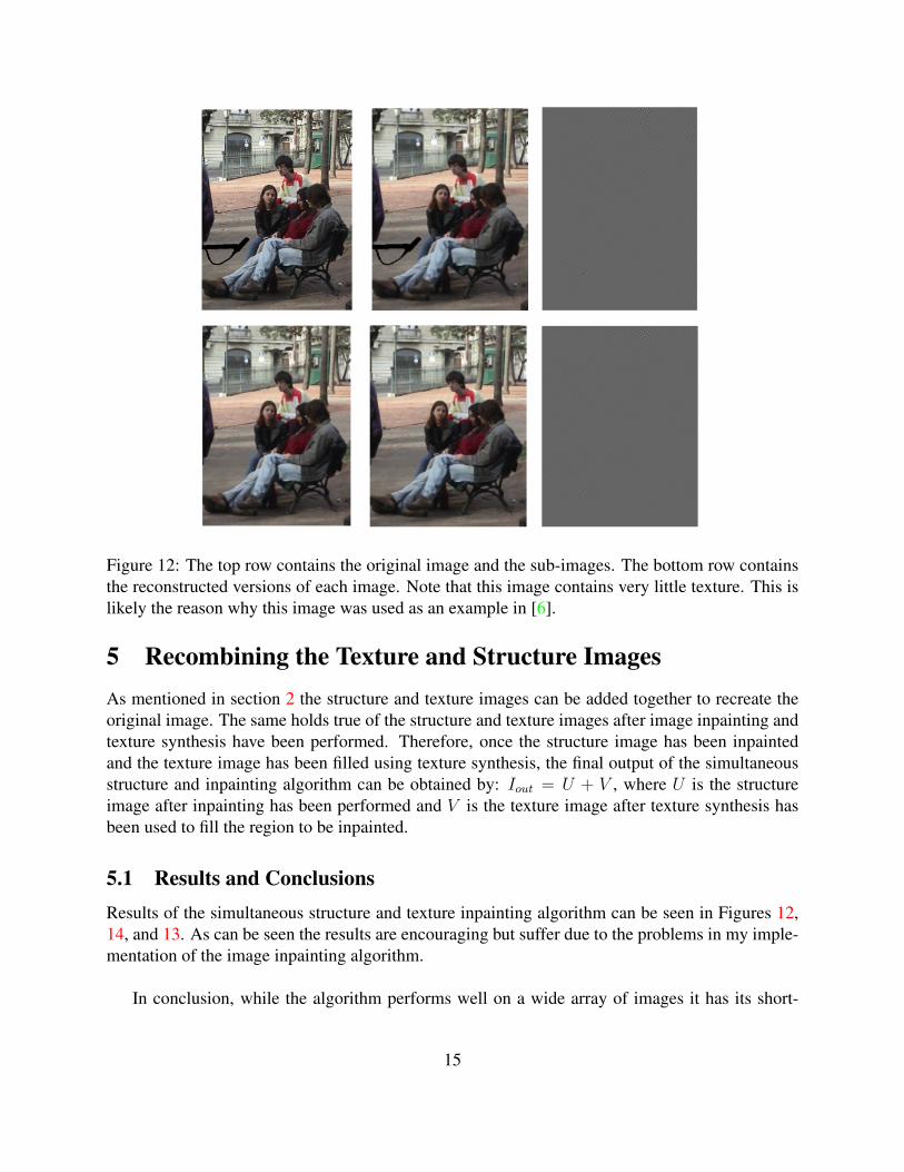
Figure 12: The top row contains the original image and the sub-images. The bottom row containsthe reconstructed versions of each image. Note that this image contains very little texture. This islikely the reason why this image was used as an example in [6].

5 Recombining the Texture and Structure ImagesAs mentioned in section 2 the structure and texture images can be added together to recreate theoriginal image. The same holds true of the structure and texture images after image inpainting andtexture synthesis have been performed. Therefore, once the structure image has been inpaintedand the texture image has been filled using texture synthesis, the final output of the simultaneousstructure and inpainting algorithm can be obtained by: Iout = U + V , where U is the structureimage after inpainting has been performed and V is the texture image after texture synthesis hasbeen used to fill the region to be inpainted.

5.1 Results and ConclusionsResults of the simultaneous structure and texture inpainting algorithm can be seen in Figures 12,14, and 13. As can be seen the results are encouraging but suffer due to the problems in my imple-mentation of the image inpainting algorithm.

In conclusion, while the algorithm performs well on a wide array of images it has its short-

15

Figure 13: The top row contains the original image and the sub-images. The bottom row containsthe reconstructed versions of each image

comings. One shortcoming is the necessity to tune several parameters. Even the tuning of threeparameters prevents the algorithm from being useful enough to the average user, inhibiting itsability to be used in a commercial software package such as Adobe Photoshop. In addition, thealgorithm is difficult to implement due to the vagueness of the anisotropic diffusion that must beused. As my experience has shown the specifics of the anisotropic diffusion used in the imageinpainting algorithm make an enormous difference on the performance of the algorithm. Withoutknowledge of the specific anisotropic diffusion used by the authors an implementation that has re-sults comparable to theirs proves elusive. In the end, this project was a worthwhile experience andI am glad to have learned much about these fields of image processing of which I was previouslyignorant.

References[1] R. Acar and C. Vogel. Analysis of bounded variation penalty method for ill-posed problems, 1994. 5

[2] F. Andreu, C. Ballester, V. Caselles, and J. Mazon. Minimizing total variation flow, 1998. 5

[3] G. Aubert and L. Vese. A variational method in image recovery. SIAM Journal on Numerical Analysis,34(5):1948–1979, 1997. 6

[4] C. Ballester, M. Bertalmio, V. Caselles, G. Sapiro, and J. Verdera. Filling-in by joint interpolation ofvector fields and grey levels, 2000. 4

[5] M. Bertalmio, A. Bertozzi, and G. Sapiro. Navier-stokes, fluid dynamics, and image and video in-painting, 2001. 4

[6] M. Bertalmio, G. Sapiro, V. Caselles, and C. Ballester. Image inpainting. 2000. 4, 7, 15

[7] M. Bertalmio, L. Vese, G. Sapiro, and S. Osher. Simultaneous structure and texture image inpainting,2002. 3, 12

[8] J. D. Bonet. Multiresolution sampling procedure for analysis and synthesis of texture images. Com-puter Graphics, 31(Annual Conference Series):361–368, 1997. 12

16

Figure 14: The top row contains the original image and the sub-images. The bottom row containsthe reconstructed versions of each image

17

[9] R. Cant and C. Langensiepen. A multiscale method for automated inpainting, 2003. 4

[10] F. Catte, P. L. Lions, J. M. Morel, and T. Coll. Image selective smoothing and edge detection bynonlinear diffusion. SIAM J. Numer. Anal., 29(1):182–193, 1992. 11

[11] A. Chambolle and P. Lions. Image recovery via total variation minimization and related problems,1997. 5

[12] A. A. Efros and T. K. Leung. Texture synthesis by non-parametric sampling. In ICCV (2), pages1033–1038, 1999. 12

[13] P. Perona and J. Malik. Scale-space and edge detection using anisotropic diffusion. 11

[14] K. Popat and R. Picard. Novel cluster-based probability model for texture synthesis, classification, andcompression, 1993. 12

[15] J. Portilla and E. P. Simoncelli. Texture modelling and synthesis using joint statistics of complexwavelet coefficients. In IEEE Workshop on Statistical and Computational Theories of Vision, 1999. 12

[16] L. Rudin, S. Osher, and E. Fatemi. Nonlinear total variation based noise removal algorithms, 1992. 5,6

[17] L. Vese. A study in the bv space of a denoising-deblurring variational problem. 5

[18] L. Vese and S. Osher. Modeling textures with total variation minimization and oscillating patterns inimage processing, 2002. 3, 4, 6

18