Edward I. Altman The Anatomy of the High Yield Bond Marketpages.stern.nyu.edu/~ealtman/anatomy.pdf · September 1998 The Anatomy of the High Yield Bond Market 3 Until the last few

Edward I. AltmanProfessor of Finance(212) [email protected].

New York UniversityStern School ofBusiness and Advisor toSalomon Smith Barney’sGlobal Corporate BondResearch Group.

SEPTEMBER 21, 1998

The Anatomy of the High YieldBond MarketAfter Two Decades Of Activity—Implications For Europe*

Until the last few years, the high yield bond market wasessentially a solely U.S. capital market phenomena. That thisnon-investment grade, fixed income asset class has grown soimpressively in the U.S. and now is possibly on the verge of anexplosion of new issuance in Europe is primarily based on asimple summary performance statistic -- an average annual netreturn to investors of about 250 basis points per year above therisk-free rate for the past two decades. But, just as the U.S. highyield market rebounded from its debacles in the late 1980's andthe Mexican Eurobond market from its peso crisis in early 1995,the long-term key factor in Europe will be the fundamental healthof firms issuing bonds. Despite short-term gyrations and flightsto quality, there is still no substitute for careful and objectiveanalysis of the underlying firms and securities that comprise themarket.

*Please note that this is a preliminary version. Please do notquote without permission of author.

September 1998 The Anatomy of the High Yield Bond Market

2

Summary Market Performance of High Yield Bonds 3

Risk and Returns.............................................................................................................................. 4

Returns and Volatility ...................................................................................................................... 6

Correlation of Returns with Other Asset Classes .............................................................................. 7

Traditional Measures of Default Rates and Losses............................................................................ 7

Historical Default Rates ................................................................................................................... 7

Promised Yield vs. Expected Default Losses: A Breakeven Analysis ................................................ 10

Defaults On High Yield Bonds Rise in First-Half Of 1998 — Still Below Average........................... 12

New Issue Bias................................................................................................................................. 13

The Mortality/Aging Approach ........................................................................................................ 13

Mortality Rates and Losses............................................................................................................... 14

Growth in Market Size..................................................................................................................... 16

Some Trends in U.S. High Yield Debt Issuance................................................................................ 17

High Yield Activity in Europe: The Time Has Come........................................................................ 18

Near Term Opportunities and Risks ................................................................................................. 19

References 20

Contents


3

Until the last few years, the high yield bond market was essentially a solely U.S.capital market phenomena. That this non-investment grade, fixed income asset classhas grown so impressively in the U.S. and now is possibly on the verge of anexplosion of new issuance in Europe is primarily based on a simple summaryperformance statistic — an average annual net return to investors of about 250basis points per year above the risk-free rate for the past two decades. Figure 1shows that over the period 1978-1997, U.S. high yield bonds promised, on average, ayield spread of 436 basis points (4.36%) more than 10-year U.S. Treasuries and, infact, returned a compound average return of 2.47% per year (2.26% arithmeticaverage). The absolute average annual return was 12.36% over this 20-year period.1

Appendices A and B illustrate the absolute and relative return performance ofhigh yield bonds for various annual starting and ending points over the 20-yearperiod 1978-1997. Note that in almost all cases the absolute compound annualaverage return is in double-digits, mostly in the 10-12% per year range. Therelative returns vary more widely. Ever since the early 1990’s, compound annualaverage return spreads have been significantly positive and as of the end of 1997,range between 0.99% and 7.22% per year, depending upon the starting date. Asnoted above, the rate for the entire period is 2.47%.

1 In the first seven months of 1998, high yield bonds returned 5.99% to investors, compared to16.46% on the S&P 500 Stock Index. Although far outdistanced by the stock market in the last threeand a half years (1995-1998), high yield bonds have had a respectable aggregate growth of 57% andan average annual (1995-1997) return of 14.60%. Similar stock market return growth rates in Europehave been achieved in what many now perceive as a fully priced, perhaps overpriced, equity market.The precipitous fall in most financial markets in August 1998 caused both the high yield and S&Pmarkets to register slightly negative returns for the first eight months of 1998.

Summary Market Performance of High Yield Bonds


4

Figure 1 . Annual Returns, Yields And Spreads On Ten-Year Treasury (Treas) And High Yield (HY) Bonds (1978 - 1997)

RETURN(%) PROMISED YIELD(%) *

YEAR HY TREAS SPREAD HY TREAS SPREAD

1997 12.83 11.16 1.67 8.86 5.75 3.11

1996 11.06 0.04 11.02 9.41 6.44 2.97

1995 19.91 23.58 (3.67) 9.70 5.58 4.12

1994 (1.17) (8.29) 7.13 11.27 7.83 3.44

1993 17.18 12.08 5.11 9.61 5.80 3.81

1992 18.16 6.50 11.66 11.28 6.69 4.59

1991 34.58 17.18 17.40 13.11 6.70 6.41

1990 (4.36) 6.88 (11.24) 17.58 8.83 8.75

1989 1.62 15.99 (14.37) 15.41 7.93 7.48

1988 13.47 9.20 4.27 13.95 9.00 4.95

1987 4.67 (2.67) 7.34 12.66 8.75 3.91

1986 16.09 24.08 (7.99) 14.45 9.55 4.90

1985 22.51 31.54 (9.03) 15.40 11.65 3.75

1984 8.50 14.82 (6.32) 14.97 11.87 3.10

1983 21.80 2.23 19.57 15.74 10.70 5.04

1982 32.45 42.08 (9.63) 17.84 13.86 3.98

1981 7.56 0.48 7.08 15.97 12.08 3.89

1980 (1.00) (2.96) 1.96 13.46 10.23 3.23

1979 3.69 (0.86) 4.55 12.07 9.13 2.94

1978 7.57 (1.11) 8.68 10.92 8.11 2.81

ARITHMETIC ANNUAL AVERAGE:

1978-1997 12.36 10.10 2.26 13.18 8.82 4.36

COMPOUND ANNUAL AVERAGE:

1978-1997 11.88 9.41 2.47

* End of year yields. Source: Altman & Waldman, 1998.

The return statistics are based on a total return method that is impacted by amultitude of factors, e.g., interest rate changes, business and credit cycles and,probably most importantly, defaults, (and recoveries after default). Indeed, if onesubtracts the average annual loss to investors from defaults of 2.18% (Figure 2 —last column) from the promised average yield spread

(4.36%), the result is very close to the annual average return spread. While it isprobably an oversimplification to look only at promised yields and expected defaultlosses, the fact of the matter is that investors in a diversified portfolio of high yieldbonds, those rated below BBB- (Standard & Poor’s, Fitch IBCA and Duff & Phelps)or Baa3 (Moody’s), did not really need to consider other factors. To complete the riskpicture, however, three other factors do need to be considered, e.g., interest rate,liquidity and currency risk (for foreign investors), but over the long run these otherfactors do not seem to add much to the story.

Risk and ReturnsFrom Figure 1, we can also observe the impact of interest rate risk on bondperformance in a clear and fundamental way. Due to their higher coupon rates, highyield bonds have shorter expected durations than comparable maturity U.S.Treasuries, and this means their price changes, due to actual interest rate changes,will probably be less dramatic. And they are! Note that Treasuries had consistently


5

lower returns in the late 1970’s and early 1980’s as interest rates climbedprecipitously. The reverse can be observed in the following years 1982-1986 (exceptfor 1983) as interest rates dropped. Hence, during relatively benign credit periods,major shifts in interest rates will drive the market. Of course, in dramatic defaultperiods, credit issues may dominate, e.g., 1989 and 1990 and, ironically, in 1991when both returns and defaults were at record high levels in the same year.2 Inaddition, short-term flight-to-quality periods, (e.g., October 1987 and August 1998),will negatively impact returns on high yield bonds.

Figure 2. Default Rates And Losses (A) (1978 - 1997)

PAR VALUE PAR VALUE

OUTSTANDING

(a)

OF DEFAULT DEFAULT WEIGHTED PRICE WEIGHTED DEFAULT

YEAR ($ MMs) ($ MMs) RATE (%) AFTER

DEFAULT

COUPON (%) LOSS (%)

1997 $335,400 $4,200 1.25% $54.2 11.87% 0.65%

1996 $271,000 $3,336 1.23% $51.9 8.92% 0.65%

1995 $240,000 $4,551 1.90% $40.6 11.83% 1.24%

1994 $235,000 $3,418 1.45% $39.4 10.25% 0.96%

1993 $206,907 $2,287 1.11% $56.6 12.98% 0.56%

1992 $163,000 $5,545 3.40% $50.1 12.32% 1.91%

1991 $183,600 $18,862 10.27% $36.0 11.59% 7.16%

1990 $181,000 $18,354 10.14% $23.4 12.94% 8.42%

1989 $189,258 $8,110 4.29% $38.3 13.40% 2.93%

1988 $148,187 $3,944 2.66% $43.6 11.91% 1.66%

1987 $129,557 $7,486 5.78% $75.9 12.07% 1.74%

1986 $90,243 $3,156 3.50% $34.5 10.61% 2.48%

1985 $58,088 $992 1.71% $45.9 13.69% 1.04%

1984 $40,939 $344 0.84% $48.6 12.23% 0.48%

1983 $27,492 $301 1.09% $55.7 10.11% 0.54%

1982 $18,109 $577 3.19% $38.6 9.61% 2.11%

1981 $17,115 $27 0.16% $12. 15.75% 0.15%

1980 $14,935 $224 1.50% $21.1 8.43% 1.25%

1979 $10,356 $20 0.19% $31. 10.63% 0.14%

1978 $8,946 $119 1.33% $60. 8.38% 0.59%

ARITHMETIC AVERAGE 1978-1997: 2.85% $42.9 11.48% 1.83%

WEIGHTED AVERAGE 1978-1997: 3.34% 2.18%

Note: (a) Excludes defaulted issues. Source: Altman & Waldman, 1998.

Liquidity risk is very difficult to quantify but is certainly present amongst the highyield bond sector compared to government bonds. This is particularly true when theinvestor institutional group is dominated by open-end mutual funds who may need tosell all at once when prospects become very uncertain and/or redemptions are high.This possibility was evident in recent years but the advent of securitized instrumentsthat pool large numbers of high yield bonds into less-vulnerable-to-liquidity assets hasmitigated that situation somewhat. And, as the trading and new issue environmentamongst the larger investment and commercial banks have become more competitive

2 This was caused by the gross over-reaction of the market in 1990 when prices of almost all highyield "junk" bonds suffered due to the over-discounting that took place.


6

since the demise of Drexel Burnham in 1990, spreads and fees have diminished aswell.

The final risk component, currency fluctuations, has involved the non-U.S. investoronly and is now becoming relevant for the U.S. and other non-European investors inthe Euro-denominated high yield debt market. To the extent that the Euro will be astable, major currency going forward from 1999, this risk will not be a major factorfor European investors.

Returns and VolatilityInvestors care not only about their realized absolute and relative asset returns, butalso about how volatile those returns have been and can be in the future. One of thestandard measures of investor risk is the ratio of realized return spreads vs. theassociated standard deviation of return - - the so-called “Sharpe Ratio.” Among themajor asset classes, high yield bonds performed best by this measure over the pastdozen years (Figure 3) and second best to the relatively new market for syndicatedleveraged loans (the high yield bond counterpart in the bank loan market) over theperiod 1992-1997.

Figure 3. Returns, Standard Deviations, and Sharpe Ratios Selected Asset Categories, 1985 - 1997

Three-Month Ten-Year Mortgage- High Grade High Yield S&P 500

Treasury Bill Treasuries Backed Corporate Bonds Stock

Mean Monthly Return (%) 0.50 0.83 0.83 0.89 1.02 1.48

Standard Deviation 0.15 1.32 2.25 1.55 1.50 4.21

Sharpe Ratio1 N/A 0.25 0.15 0.25 0.34 0.23

1 Total return minus Return on 91-Day Treasury Bill/standard Deviation of total Return

Source: Standard & Poor’s, Salomon Smith Barney Inc.

One important caveat that must be made when citing the Sharpe Ratio, or any othermeasure that uses a mean-variance approach, is the assumption of a symmetric returndistribution with known properties surrounding the various moments of distribution.For high yield bonds, just like all credit assets, we know that the long-termdistribution of returns is not normal since the investor has limited upside potential andcan only achieve the promised return, or slightly higher if the issue is called at apremium or the credit quality level migrates upward. And, the early redemption of anissue for those investors who trade high yield securities, as opposed to the buy andhold investor, further limits the upside potential. But, the possible loss is great in caseof default that is accompanied by a low or negligible default recovery. In fact, defaultrecoveries average about 40% of face value (see Figure 2 and our discussion ondefaults at a later point). In summary, high yield bonds have performed extremelywell over the past two decades, although this class of assets’ superiority, on a risk-adjusted basis, is probably overstated due to the bias discussed above.

Within the non-investment grade sector, the expected positive relationship betweenrisk and return manifests, with Double-B’s having the lowest return (slightly over12%) followed by single-B’s and the highest absolute returns for triple-C’s. These arelong-term relationships and do not manifest every year. Sharpe ratios, however,indicate the reverse, with double-B bonds the leader by far and single-B and triple-B


7

(the lowest of the investment grade classes) tied for second place, and triple-C’strailing.

Correlation of Returns with Other Asset ClassesInvestors who participate in a number of asset groups will be concerned with howeach classes’ returns correlate with all others - - actual or potential. High yield bondstend to have average correlations, i.e., in the .40 to .55 range, with most other majorasset classes (Figure 4).

Figure 4. Correlation of Monthly Returns Selected Asset Categories, 1985 - 1997

High Yield Mortgage- 10-Year 3-Month S&P NASDAQ High Grade

Backed Treasuries Treasuries Stocks Stocks Corporate

High Yield 1.000

Mortgage-Backed 0.460 1.000

Ten-Year Treasuries 0.426 0.889 1.000

Three-Month Treasuries -0.004 0.350 0.301 1.000

S&P 500 Stocks 0.526 0.318 0.361 0.040 1.000

NASDAQ Stocks 0.551 0.187 0.213 -0.048 0.863 1.000

High Grade Corporate 0.550 0.911 0.953 0.275 0.413 0.275 1.000

Sources: National Association of Securities Dealers, Standard & Poor’s, Salomon Smith Barney Inc.

The long-run performance of high yield bonds has provided superior returns andreasonable diversification attributes - - especially with their relatively mediumcorrelations with low default risk bonds and only slightly higher correlations withcommon stocks. The latter might surprise casual observers since high yield bondshave a reputation of being quasi-equities. Indeed, this is true, but only for the mostrisky of the high yield sectors — low single-B’s and triple-C’s.

Traditional Measures of Default Rates and LossesAccurate measurement of default risk is, of course, critical to the task of determiningthe required risk premiums on bonds of different credit quality and evaluating thereturns on those securities. The traditional method that I have followed to measureannual default rates is based on comparing the dollar amount of all issues defaultingin a given year divided by the dollar value of all bonds outstanding as of some pointduring the year. For any given category of bonds, the annual default rates are thenaggregated over some longer time horizon to provide an estimate of the average yearlyrate of default.

Historical Default RatesAppendix C shows the average annual default rate, calculated using the methoddescribed above, for below investment-grade debt for the period 1971-1998 (firsthalf). Weighted average default rates for various periods are shown below (Figure 5).Note that the weighted average default rate was 3.31% over the entire 28-year period(1971-1997) and the arithmetic (unweighted) average annual rate is 2.61%. The lastsix years’ (1992-1997) weighted average annual rate is 1.61%. The median rate forthe entire sample period is 1.50% per year.


8

The standard deviation of our annual default rate series was about 3.0%, whichtranslates into about a 2.5% probability of observing an annual default rate above9.3% - - two standard deviations above the mean. Indeed, we have observed that thedefault rate was above 9.3% on two occasions out of the 29 years in our time series.Those two outlier years were 1990 and 1991, when the combination of highlyleveraged corporate restructurings of the late 1980’s, that were financed withexcessive levels of debt, and a business recession with a poorly performing stockmarket caused this massive increase in defaults. And, as noted earlier, the second ofthese years (1991) was accompanied by phenomenal returns for high yield investorsdue to the market over-estimation of future default rates in 1991 and beyond.

Figure 5. Average Annual Default Rates for Various Periods (1971 - 1997)

1971 - 1997 1978 - 1997 1992 - 1997

Weighted Average 3.311% 3.343% 1.607%

Default Rate(1) (3.048%) 3.160%) (0.484%)

Arithmetic Average 2.613% 2.850% 1.723%

Default Rate(2) (2.554%) (2.660%) (0.753%)

Median Default Rate 1.500% 1.605% 1.353%

(1)Weighted by the amount of High Yield Debt Outstanding in each year.(2)Unweighted; Each Year has Equal Weight.

Standard Deviation in Parentheses.

Source: Appendix C.

An alternative, traditional measure of annual default rates is provided by Moody’strailing 12-month average rate, as indicated in Appendix D. This non-weighted ratefor the same period averaged 3.20% per year, based on principal amount outstandingand 3.36% per year, based on percent of issuers outstanding. Hence, the results fromboth Moody’s and our default rate methods are quite similar.

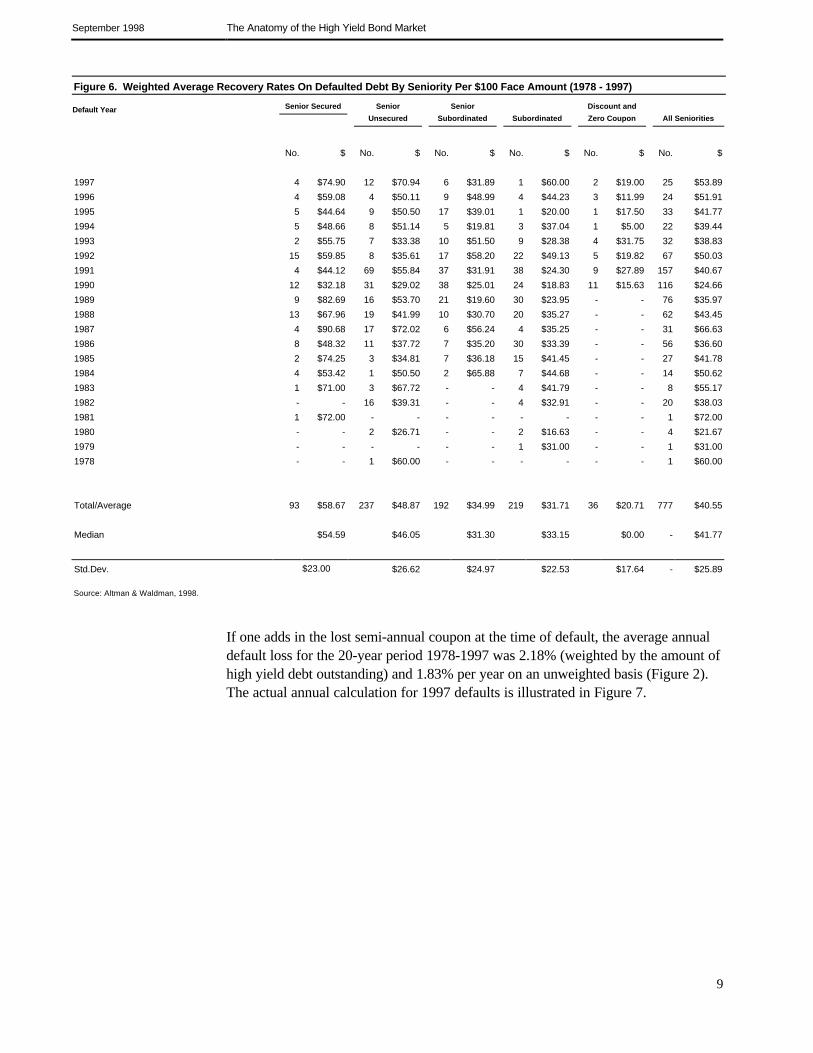
An even more relevant default statistic for most high yield bond investors is theproportion of the portfolio that is lost due to defaults. The use of default rates alone tomeasure losses assumes that the value of defaulting bonds is zero when the position isliquidated — usually assumed to be just after default. In reality, however, defaultedbonds sell at substantial prices just after default and even higher prices, for mostseniorities, upon the resolution of the restructuring process (usually upon emergencefrom the Chapter 11 bankruptcy reorganization). Figure 6 indicates that, for a sampleof 777 defaulting bonds from 1978-1997, the average recovery rate, based on theprice of the bonds just after default, was $40.55 on an equivalent face value of$100.00. Note that the recovery rate varies according to the bonds’ seniority withsenior secured bonds the highest at about 59 cents on the dollar, down to subordinatedissues of 32 cents and discounted bonds of 21 cents. In Altman and Kishore (1996),we also have observed recovery rates by industrial sector. These recovery figures canbe interpreted as the market’s best guess about the eventual recovery, discounted backto the default date. A study by Altman and Eberhart (1994) concluded that the marketprobably has underestimated recoveries on senior secured and senior unsecured issuesand has overestimated recoveries on the more junior seniorities, i.e., higher senioritiesperform best in the restructuring period.


9

Figure 6. Weighted Average Recovery Rates On Defaulted Debt By Seniority Per $100 Face Amount (1978 - 1997)

Default Year Senior Secured Senior

Unsecured

Senior

Subordinated Subordinated

Discount and

Zero Coupon All Seniorities

No. $ No. $ No. $ No. $ No. $ No. $

1997 4 $74.90 12 $70.94 6 $31.89 1 $60.00 2 $19.00 25 $53.89

1996 4 $59.08 4 $50.11 9 $48.99 4 $44.23 3 $11.99 24 $51.91

1995 5 $44.64 9 $50.50 17 $39.01 1 $20.00 1 $17.50 33 $41.77

1994 5 $48.66 8 $51.14 5 $19.81 3 $37.04 1 $5.00 22 $39.44

1993 2 $55.75 7 $33.38 10 $51.50 9 $28.38 4 $31.75 32 $38.83

1992 15 $59.85 8 $35.61 17 $58.20 22 $49.13 5 $19.82 67 $50.03

1991 4 $44.12 69 $55.84 37 $31.91 38 $24.30 9 $27.89 157 $40.67

1990 12 $32.18 31 $29.02 38 $25.01 24 $18.83 11 $15.63 116 $24.66

1989 9 $82.69 16 $53.70 21 $19.60 30 $23.95 - - 76 $35.97

1988 13 $67.96 19 $41.99 10 $30.70 20 $35.27 - - 62 $43.45

1987 4 $90.68 17 $72.02 6 $56.24 4 $35.25 - - 31 $66.63

1986 8 $48.32 11 $37.72 7 $35.20 30 $33.39 - - 56 $36.60

1985 2 $74.25 3 $34.81 7 $36.18 15 $41.45 - - 27 $41.78

1984 4 $53.42 1 $50.50 2 $65.88 7 $44.68 - - 14 $50.62

1983 1 $71.00 3 $67.72 - - 4 $41.79 - - 8 $55.17

1982 - - 16 $39.31 - - 4 $32.91 - - 20 $38.03

1981 1 $72.00 - - - - - - - - 1 $72.00

1980 - - 2 $26.71 - - 2 $16.63 - - 4 $21.67

1979 - - - - - - 1 $31.00 - - 1 $31.00

1978 - - 1 $60.00 - - - - - - 1 $60.00

Total/Average 93 $58.67 237 $48.87 192 $34.99 219 $31.71 36 $20.71 777 $40.55

Median $54.59 $46.05 $31.30 $33.15 $0.00 - $41.77

Std.Dev. $23.00 $26.62 $24.97 $22.53 $17.64 - $25.89

Source: Altman & Waldman, 1998.

If one adds in the lost semi-annual coupon at the time of default, the average annualdefault loss for the 20-year period 1978-1997 was 2.18% (weighted by the amount ofhigh yield debt outstanding) and 1.83% per year on an unweighted basis (Figure 2).The actual annual calculation for 1997 defaults is illustrated in Figure 7.


10

Figure 7. 1997 DEFAULT LOSS RATE

BACKGROUND DATA

AVERAGE DEFAULT RATE 1997 1.252%

AVERAGE PRICE AT DEFAULT (a) 54.246%

AVERAGE LOSS OF PRINCIPAL 45.754%

AVERAGE COUPON PAYMENT 11.867%

DEFAULT LOSS COMPUTATION

DEFAULT RATE 1.252%

X LOSS OF PRINCIPAL 45.754%

DEFAULT LOSS OF PRINCIPAL 0.573%

DEFAULT RATE 1.252%

X LOSS OF 1/2 COUPON 5.933%

DEFAULT LOSS OF COUPON 0.074%

DEFAULT LOSS OF PRINCIPAL AND

COUPON

0.647%

(a) If default date price is not available, end-of-month price is used. Source: Altman & Waldman, 1998.

Finally, it is important to mention that bondholders lose not only from defaults, butalso in cases of financial distress that do not result in a legal default but rather indistressed exchange arrangements. Our default statistics include distressed exchanges,whereby creditors accept cash and/or securities of lower value and lower interest ratesthan originally promised. Of late, these distressed exchange, out-of-courtarrangements are being replaced, in many cases, by so-called “prepackaged Chapter11 bankruptcies” where the exchange takes place under the less stringent votingrequirements of the U.S. Bankruptcy Code.

Promised Yield vs. Expected Default Losses: A Breakeven AnalysisWe have shown that, over the last two decades, the promised yield spread on U.S.high yield bonds has averaged almost two and a half (2 1/2%) percent per annummore than the annual loss incurred from defaults. In order to better understand thisrelationship, the following formula and discussion illustrates a required yield onbonds in order to breakeven vs. default-risk-free Government bonds. One can thenobserve the actual current promised yields compared to the breakeven yield to assessthe relative attractiveness of the market at any point in time.


11

where:

BEYt = Breakeven Yield in Period t.

Rf = Yield on Default Risk Free U.S. Treasury Bonds.

Df = Expected (or Average Annual) Default Rate

Rec = Expected (or Average Annual) Default Recovery Rate

HYC = High Yield Coupon Rate on Defaulted Bonds.

If the following conditions and investor expectations exist,

Risk Free Rate (Rf) = 6.0%

Expected Annual Default Rate (Df) = 3.0%

Expected Recovery Rate on Defaults (Rec) = 40.0%

Coupon Rate on Defaulting High Yield Bonds (HYC) = 12.0%

then the resulting promised yield to maturity that would result in a breakevensituation (BEY) is 8.23%. Note that the promised yield is earned only on theproportion of the market that does not default — hence the denominator in ourformula subtracts the default rate from one (1.0). If the current yield on a diversifiedportfolio of bonds is greater than the breakeven yield, then a positive return spreadcan be expected. The greater the difference between the promised yield and thebreakeven rate, the higher one can expect the return to be. This analysis assumes nochange in interest rates over the relevant horizon. As of September 1, 1998, thepromised yield to maturity on high yield debt was 11.02% and the 10-year risk freerate was 5.04% (an enormous spread of almost six percent). Assuming the historicaverage default (3.3%) and recovery (40.0%) rates as reasonable expectations, thebreakeven yield calculates at 7.47% and the differential between the promised andbreakeven yield equaled 3.55%. This implies a strong positive indication forsubsequent high yield returns.

In Altman and Bencivenga (1995), we examined the statistical relationship betweenthe current minus the breakeven rates and the subsequent six and twelve-month

)1(

)2

()1(

f

fecff

t D

HYCDRDR

BEY−

+−+

=


12

realized returns on high yield bonds, as well as BBB, BB, and B rated bonds, and theresults were positive and significant. The formula can also be used to “back-out” theimplied default rate that the market consensus is expecting by solving for the defaultrate that results in the current yield equaling the breakeven rate. As of September 1,1998, that rate was . An alternative way to look at the differential between thebreakeven yield spread and current yield spread is the yield premium that investorsrequire for liquidity risk and also the fact that they could be wrong about theirexpectations of default and recovery rates. The latter considerations known as theunexpected loss, is a common and relevant consideration in bank lending models

Defaults On High Yield Bonds Rise in First-Half Of 1998 — Still Below AverageThe long anticipated rise in default rates and losses in the high yield corporate bondmarket appears to have started in the first-half of 1998. Defaults and distressedexchanges in the straight (non-convertible), non-investment grade U.S. bond marketwere $3.7 billion in the first six months of 1998 compared to $2.4 billion in the firstsix months of 1997 and $4.2 billion for the entire 1997. The number of defaultingissues and issuers also rose to 26 and 19 respectively, compared to 12 and 8respectively in the first six months of 1997, almost equaling the totals of 29 and 21for all of last year. In addition, the amount of Eurobond issue defaults (not included inour default rate calculation), swelled dramatically, with the Asian market (e.g.,Indonesia, Korea) contributing the vast majority of non-U.S. defaulting issues.Moody’s default rates do include international defaults that are rated by that agency.Incidentally, it is extremely difficult to estimate expected default losses in emergingmarkets due to the lack of historical data, lack of ratings, and particularly highlyuncertain restructuring and bankruptcy processes.

Our traditional default rate calculation, measured by the face value of defaultsdivided into the population of high yield bonds as of the start of 1998, was 0.99%(Figures Error! Reference source not found.) compared to 0.83% for the first sixmonths of 1997 and 1.25% for the entire past year. The increase in the first-halfdefault rate occurred despite a significant increase in the base population to $379billion.

Simple extrapolation of the first half default rate experience would yield a default rateof about 2% for all of 1998. Despite this considerable increase from last year, andfrom the average for the last five years as well, the rate of default of high yield bondswill still be far below the 1971-1997 long-term weighted average of 3.3%. Notsurprisingly, default losses also increased significantly in 1998, as the default rateclimbed and the recovery rate dipped considerably. The weighted (by face value)average recovery rate, as measured by the price just after default (or the distressedexchange basis), fell from last year’s 54.2% to the 1998 first half level of 38.9%. Theresulting default loss, which includes the loss of a semi-annual coupon payment was0.65% (65 basis points). This loss was approximately equal to the loss for the entireyear 1997. If we extrapolate the loss from defaults for the entire year 1998, the result(1.3%) is still below the historical average of 2.2%.

We have often observed an inverse relationship between the change in default ratesand the change in recovery rates. More careful analysis of this phenomenon is in theworks.


13

New Issue BiasWe are certainly aware that a booming new issue high yield bond market will biasdownward our traditional annual default rate calculation since the denominator is theface value outstanding of the market at the start of the calculation period. In 1997,almost $120 billion of publicly registered and 144a high yield bonds were issued andthe base population increased by over $44 billion (net of redemption and ratingchanges) to $379 billion (the population has increased to over $475 at the end of thefirst half of 1998). Thus, our 1997 and 1998 default rate and loss calculations will bedownward biased since these new issues, with rare exception, do not default withinthe first year. This short-term bias motivated us, in part, to create the mortality rateapproach (see below) which is sensitive to the aging effect.

The Mortality/Aging ApproachAlthough the traditional method for assessing default rates and losses hasconsiderable relevance for measuring bond performance, it also has potential biases.Because of such biases, the most recent default history — while immensely useful toportfolio managers and other investment officers in projecting near-term expectedlosses and setting aside adequate reserves to cover such losses — may turn out tohave been an unreliable basis for assessing longer-term losses.

Why is that so? First of all, as with all historical studies, it could be suggested thatthe near-term future is not likely to repeat the average or near-term past. Both thenumerator (that is, the amount of annual defaults) and the denominator (the amount ofbonds outstanding) in the default rate ratio will surely change in the future. And, ifthe amount of high yield bonds outstanding fails to increase as it has in the past (oreven falls, as it did in 1992 and 1993), while the amount of defaults continues togrow, then default rates and investor losses will rise above the historical levelsreported using the traditional approach.

We have also argued, however, that the opposite could take place. That is, as newissues rise from depressed levels and as defaults arising from past excesses arepurged from the market, default rates in certain years, e.g., 1990 and 1991, measuredtraditionally, are likely to be overestimates of the future rates owing to this same bias.

A related criticism of the traditional method for calculating default rates is its failureto consider the possibility that the likelihood of default actually changes with the ageof the bond. In putting all junk bonds outstanding at a given point in time in the samebasket, the average annual method effectively assumes that the probability of defaultfor a newly-issued bond of a certain rating is identical with that of a bond of thatsame rating that has been outstanding for, say, five years. But if it is true that theprobability of default rises with age — especially in the case of junk bonds where thebetter firms often call-in the bonds after 3-5 years — then default rates on newly-issued bonds should rise after a few years.

Briefly stated, the basic contention is this: because of the rapid growth of the junkbond market during the 1980s, and again in the mid to late 1990s, use of thetraditional methods for measuring defaults could blind investors to the reality thateffective default rates could rise well above current reported levels.


14

While the aging argument has some intuitive appeal, the more important reason forthe considerable rise in default rates in 1990 and 1991 was the debt excesses of 1987-1989 caused by the incredibly high premiums paid for corporate restructures, e.g.,LBOs. Combined with declining asset sales and values and the lack of refinancingalternatives, the highly leveraged, e.g., debt to equity ratios of 6:1 and above,corporate restructurings disappeared after 1989 and defaulting LBOs becameincreasingly more common. While LBOs have reappeared in the mid-to-late 1990’s,the proportion of equity in the restructured firms’ capital structure has beenconsiderably higher — about 30% — leading to more prudent leverage and a betterchance that the high debt amounts will be successfully refinanced, if necessary, orpaid down.

A final point on this aging effect question reminds us that when a firm issues newbonds, the significant inflow of cash is usually sufficient to make several couponpayments, regardless of the operating performance of the company. It is only after 2-3years of dismal performance can we expect defaults to occur with any regularity for aparticular rating class of bonds. Of course, if the cash is used entirely to refinance anexisting debt outstanding, then excess cash for future interest payments would not beavailable.

Mortality Rates and Losses

The joint queries on a bond’s aging effect and the search for default rates on specificrating classes, e.g., BB, B, etc., lead us to develop the mortality approach for defaultrate measurement. Simply put, mortality rates on corporate bonds is an actuarially-based technique that adjusts for changes over time in the size of the original sample ofnewly-issued bonds, of a given bond rating, due to defaults, calls and scheduledredemptions. For example, if there are $10 billion of single-B bonds issued in 1996and $200 million default in 1997, the marginal one-year rate is 2.0%; and if $300million of the same 1996 cohort defaults in 1998, the second year mortality rate ishigher 3.06%, based on the $300 million defaulting on a remaining base of $9.8billion. The cumulative two-year rate, based on the formula (below) would be$5.00%. The specific calculation for marginal mortality rates (MMR) and cumulativemortality rates (CMR) are:

and

tPeriodofStartatBondsofNumberIssuerorDollar

tPeriodinDefaultingBondsofNumberIssuerorDollarMMRt )(

)(=


15

where:

SRt = Survival rate in Period t = 1 - MMRt.

It should be made explicitly clear that we are measuring the marginal and cumulativemortality rates for bonds with specific original ratings over the relevant time periodsafter issuance. As such, we can assess the aging effect. While this method isconsistent with actuarial theory, it is different from the cohort (Moody’s) and staticpool (S&P) approaches utilized by the rating agencies for estimating bond defaults.3

Our total defaulted population that had a rating upon issuance and a price at defaultnow numbers over 650. Using the mortality methodology, we update results eachyear. Mortality rates and losses from 1971-1997 are reported in Figures Error!Reference source not found. and Error! Reference source not found.. One can observea number of important statistics from these tables. First, default rates can be assessedfor all rating classes, not just the high yield bond groups. As expected, the rates forinvestment grade bonds are quite low, although not zero. Indeed, even AAA bonds areobserved to default and when Texaco’s AA bonds defaulted in 1987, the AA rateactually jumped above the A rate.4

Note that the five- and ten-year rates for our high yield bond groups, as shown belowin Figure 8, seem to be high, but when you factor in their high promised yields, theresult is consistent with our earlier discussion of returns net of defaults. For example,the five-year single-B cumulative mortality rate is 21.95%, or about 4.0% per year.This rate is quite similar to the 3.3% annual default rate for all high yield bondsmeasured using the traditional approach. The corresponding cumulative mortality lossrate is 16.1%, or about 3.0% per year. If one considers an average annual yield

3 These approaches measure the proportion of issuers that default from different bond rating classesas of some initial date, regardless of the age of the bond. For example, all Ba bond issuers as ofJanuary 1, 1996 are observed as to their default frequency in subsequent periods. See Moody's (1998)and S&P (1998) for details and results. The three approaches for measuring corporate bond defaults,as well as rating migration patterns, are discussed and contrasted in Altman, Caouette and Narayanan(1998).4 Due to Texaco's high recovery rate, however, the mortality loss rate for AA bonds in Appendix E islower than the single-A rate -- as it should be.

[ ]tt SRCMR Π−=1


16

spread of about 5.0% per year on single-B bonds, the attractiveness of these low-rated issues becomes clearer.

Figure 8.

Cumulative Default Rates Cumulative Default Losses

Rating One-Year Five-Year Ten-Year One-Year Five-Year Ten-Year

BBB 0.03% 1.64% 2.80% 0.02% 0.53% 1.62%

BB 0.37% 8.32% 16.37% 0.24% 5.61% 10.33%

B 1.47% 21.95% 33.01% 0.85% 16.07% 23.74%

Source: Figures Error! Reference source not found. and Error! Reference source not found. and Altman and Waldman (annually).

In summary, the mortality rate and loss results provide the analyst with aconceptually correct method for assessing the expected default probability of a givennew corporate bond issue and these

probabilities are linked with the aging of the bond. We believe that mortality rateson U.S. bonds can be used in markets outside the U.S. (e.g., Europe) forassessing default rates where the market is too new to provide its own statistics.

With respect to the aging effect, one can observe that the marginal (yearly) rates forhigh yield, non-investment grade bonds does have a pronounced increasing defaultrate from original issuance up to the third year, after which the marginal rates tend tolevel off. For example, the BB marginal rates are 0.37%, 0.72% and 2.94% for years1-3 and single-B’s are 1.47%, 3.76% and 6.89% respectively. These increasingmarginal rates are consistent with the theories put forth earlier.

Cumulative default data from our mortality rate calculations, as well as similarstatistics from the rating agencies, are increasingly being used by market analysts andthe agencies themselves in evaluating individual and securitized portfolio pools ofhigh yield debt. And, in a recent study (Altman & Waldman, 1998), the mortalitymethodology was applied to syndicated leveraged bank loans with results that weresimilar to bonds for the 1991-1996 period.

Growth in Market SizeThe last two years (1996-1997) have seen unprecedented growth in new issuance andsize of the U.S. high yield bond market. New bonds, which include public registeredand 144a issues with

registration rights, totalled $66 billion and $119 billion in 1996, 1997 (Figure 9) andthe 1998 amount was running far ahead of 1997 totals until the flight to qualityreaction to global stock market and Russian economy problems in late August. Weestimate that the size of the U.S. domestic market was about $380 billion at the end of1997 and is now (September 1998) over $500 billion. Note the dramatic increase in144a issues as firms find it more convenient to tap the capital markets on a timelybasis and then follow soon after with the registration materials. In essence, publiclyregistered and 144a’s with registration rights are identical in their risk-return andcredit quality characteristics.


17

Figure 9. New Issue Volume - High Yield Bonds 1977-1997

Publi 144 Total

Year Number of Issues Principal Amount ($ Millions) Number of Issues Principal Amount ($ Millions) Number of Issues Principal Amount ($ Millions)

1977 61 $1,040.2 61 $1,040.2

1978 82 1,578.5 82 1,578.5

1979 56 1,399.8 56 1,399.8

1980 45 1,429.3 45 1,429.3

1981 34 1,536.3 34 1,536.3

1982 52 2,691.5 52 2,691.5

1983 95 7,765.2 95 7,765.2

1984 131 15,238.9 131 15,238.9

1985 175 15,684.8 175 15,684.8

1986 226 33,261.8 226 33,261.8

1987 190 30,522.2 190 30,522.2

1988 160 31,095.2 160 31,095.2

1989 130 28,753.2 130 28,753.2

1990 10 1,397.0 10 1,397.0

1991 48 9,967.0 48 9,967.0

1992 245 39,755.2 29 $3,810.8 274 45,566.0

1993 341 57,163.7 95 15,096.8 436 72,260.5

1994 191 34,598.8 81 7,733.5 272 42,332.3

1995 152 30,139.1 94 14,242.0 246 44,381.1

1996 142 30,739.4 217 35,172.9 359 65,912.3

1997 103 19,822.0 576 98,885.0 679 118,707.0

Total 2,669 395,579. 11,092 174,941.0 3,761 570.520.1

Note: Includes non-convertible, corporate debt rated below investment grade by Moody’s or Standard & Poor’s. Excludes mortgage- and asset-backed issues, as well as non-144a

private placements. Source: Securities Data Company

Some Trends in U.S. High Yield Debt IssuanceThe following appear to be recent trends that will help to shape the future risk andreturn profile of high yield bonds in the U.S.:

ä Dramatic increase in 144a issues making it easier and quicker for new issues tobe brought to and sold in the market.

ä Senior priority debt in the 1990’s becoming the dominant seniority with 60-70%of new issuance either senior secured or senior unsecured. This probably meanshigher than average recovery rates after default, but recoveries are still drivenmainly by economic prospects.

ä A slight increase in the proportion of high yield bonds issued at very low quality,i.e., B- or below. In 1997, over 25% of new issuance came to market at these lowratings. This is an additional factor indicating an increase in default rates,probably commencing in 1998.

ä Large increase in securitizations (CBOs) providing much greater liquidity forhigh yield investors and permitting additional groups of non-traditional investors


18

to participate in the market. In addition, we observe some special purposevehicles formed with both bonds and leveraged loans in the collateral pool.

High Yield Activity in Europe: The Time Has ComeThe high yield, non-investment grade bond market in Europe began quietly in 1995.In 1997, about $6 billion of new issues came to market, mostly denominated in U.S.dollars (Figure 10), and the growth in 1998 has continued to be impressive. The firstEuro denominated bond issue came to market in March 1998.5 This market willprobably grow considerably with the large number of corporations in Europe andelsewhere lacking the size and earnings predictability to obtain investment graderatings. The benefits of long-term, fixed rate debt, denominated in the new andprobably stable Euro, is an enticing market for these firms.

Among the reasons why European companies can be expected to tap this new sourceof capital are that it provides (1) a means to restructure firms that are overloaded withless flexible, more constraining bank loans by substituting fixed interest capitalmarket bonds; (2) a long-term source of capital for investment — asset growth; and(3) a growing number of firms’ independence from the central bank regulatedfinancial institutions or to free-up borrowing capacity in the future from these sameinstitutions. Indeed, Gilson and Warner (1998) argued that flexibility benefits havebeen the principal driver of high yield bond issues by public companies in the UnitedStates for the last two decades.

Combined with the demonstrated attractive promised yield and realized returnspreads, discussed earlier, and a growing comfort level for investors in this newmarket, these supply and demand factors bode well for dynamic market growth inhigh yield, fixed-rate, Euro-denominated bonds.

The demand side of the equation needs to be convinced of the attractive risk-returntrade-off.

In addition, a clearer and possibly integrated set of bankruptcy laws and creditorpriorities in Europe would help in cross-border investments. Demand coming from theUnited States and other non-European countries will help to fuel this new market.Finally, it would appear that the European Union could help to reduce the likelihoodof any individual nation’s establishing, or continuing, impediments to the corporatebond market’s growth. For example, nations will likely be less reliant on their localinstitutions and individuals financing the country’s public debt and therefore lessinclined to discourage alternative investment vehicles for those investors.

5 Cellular Communications International, a U.S. based holding company with ventures in severalEuropean companies, issued a 235 million eurobond and it was speculated (High Yield Report,March 16, 1998) that the Euro will become as popular as sterling or deutschemarks in the high yieldmarket.


19

Near Term Opportunities and RisksEurope had been mired in a prolonged recession in the early and mid-1990’s and nowseems poised to enjoy a sharp economic recovery. Inflation is historically extremelylow and interest rates and unemployment are dropping. The merging of 11countries’ currencies will lead to trade and exchange efficiencies and make crossborder investments a painless and less costly transaction. The combination ofcorporate profit and cash flow growth of over 20% in 1997 and increasingrestructuring opportunities, including the substitution of less stringent capitalmarket bonds for bank debt, bode well for the high yield market’s growth.

On the negative side, is the very recent wholesale flight to quality as conditions inRussia became chaotic and the Asian crisis continues to sap the optimism of investorsworldwide. Europe, despite its economic strengths, cannot avoid these parallelproblems. And, if the Asian crisis tips the scales toward a slow down in the UnitedStates, Europe’s economic growth will be negatively impacted and its markets,including high yield bonds, will suffer and its growth muted.

Since high yield debt and equity markets typically suffer when markets become morecredit quality conscious, the near term outlook is consequently uncertain.


20

Altman, Edward, 1989, “Measuring Corporate Bond Mortality and Performance,”Journal of Finance, 44, September, 909-922.

Altman, Edward and Scott Nammacher, 1987, Investing in Junk Bonds, John Wiley& Sons, New York.

Altman, Edward and Joseph C. Bencivenga, 1995, “For Richer or Poorer: A YieldPremium Model For the High Yield Debt Market,” Salomon Brothers Inc, March 15;and Financial Analysts Journal, “A Yield Premium Model for the High Yield DebtMarket,” September/October 1995, 49-56.

Altman, Edward and Allan Eberhart, 1994, “Do Seniority Provisions ProtectBondholders’ “Investments?”, The Journal of Portfolio Management, Summer, 67-74.

Altman, Edward and Vellore Kishore, 1996, “Almost Everything You Wanted toKnow About Recoveries on Defaulted Bonds,” Financial Analyst Journal,November/December, 57-64.

Altman, Edward and Robert Waldman, (Annually) “Defaults and Returns on HighYield Bonds,” Salomon Smith Barney Inc, New York, e.g., January 30, 1998.

Altman, Edward and Robert Waldman, 1998, “Default Rates in the Syndicated BankLoan Market: A Mortality Analysis,” January 30, 1998, Salomon Smith BarneyInc, New York.

Caouette, John, Edward Altman and Paul Narayanan, 1998, Managing Credit Risk:The Next Great Financial Challenge, John Wiley & Sons, New York.

Gilson, Stuart and Jerold Warner, 1998, “Junk Bonds, Bank Debt and FinancingCorporate Growth,” Working Paper, Harvard Business School, Cambridge, MA.

Working Paper #98-037, Harvard Business School, Cambridge, MA.

Moody’s, 1998, “Monthly Defaulted Debt Index,” Moody’s Investors Service, NewYork.

Standard & Poor’s, 1998, Rating Performance 1997: Stability and Transition,New York.

References


21

Appendix A. Compound Average Annual Returns Of High Yield Bonds (%)’1978-1996

BASETERMINAL PERIOD (DECEMBER 31)

PERIOD

(JAN 1) 1978 1979 1980 1981 1982 1983 1984 1985 1986 1987 1988 1989 1990 1991 1992 1993 1994 1995 1996 1997

1978 7.5 5.6 3.3 4.3 9.4 11.4 11.0 12.4 12.8 11.9 12.1 11.1 9.90 11.5 11.9 12.2 11.4 11.8 11.8 11.8

1979 3.6 1.3 3.3 9.9 12.2 11.6 13.1 13.4 12.4 12.5 11.5 10.1 11.8 12.2 12.5 11.6 12.1 12.0 12.1

1980 (1.0) 3.1 12.1 14.4 13.2 14.7 14.9 13.6 13.5 12.3 10.7 12.5 12.9 13.2 12.2 12.6 12.5 12.6

1981 7.5 19.3 20.1 17.1 18.1 17.8 15.8 15.5 13.9 11.9 13.8 14.1 14.4 13.2 13.6 13.5 13.4

1982 32.4 27.0 20.5 21.0 20.0 17.3 16.7 14.7 12.4 14.4 14.8 15.0 13.6 14.1 13.9 13.8

1983 21.8 14.9 17.4 17.0 14.4 14.3 12.4 10.1 12.6 11.9 13.5 12.2 12.8 12.6 12.6

1984 8.5 15.2 15.5 12.7 12.8 10.9 8.6 11.5 10.9 12.7 11.4 12.0 12.0 12.0

1985 22.5 19.2 14.1 14.0 11.4 8.6 11.9 12.7 13.2 11.7 12.4 12.3 12.3

1986 16.0 10.2 11.3 8.8 6.0 10.3 11.4 12.1 10.5 11.4 11.4 11.5

1987 4.6 8.9 6.4 3.6 9.2 10.6 11.5 9.8 10.9 10.9 11.1

1988 13.4 7.3 3.3 10.3 11.8 12.7 10.6 11.7 11.6 11.8

1989 1.6 (1.4) 9.3 11.5 12.6 10.1 11.5 11.4 11.6

1990 (4.3) 13.4 15.0 15.5 11.9 13.2 12.9 12.9

1991 34.5 26.1 23.0 16.4 17.1 16.1 15.6

1992 18.1 17.6 11.0 13.1 12.7 12.7

1993 17.1 7.6 11.5 11.4 11.7

1994 (1.1) 8.8 9.5 10.3

1995 19.9 15.4 14.5

1996 11.0 11.9

1997 12.8

Source: Merrill Lynch High Yield Master Index; Edward I. Altman, New York University Salomon Center


22

Appendix B. Compound Annual Return Spreads Between ‘High Yield And Lt Government Bonds (%)1978-1996

BASETERMINAL PERIOD (DECEMBER 31)

PERIOD

(JAN 1) 1978 1979 1980 1981 1982 1983 1984 1985 1986 1987 1988 1989 1990 1991 1992 1993 1994 1995 1996 1997

1978 8.6 6.6 5.0 5.5 3.1 5.8 4.1 2.7 1.5 2.2 2.4 0.9 (0.0) 1.0 1.7 1.9 2.3 2.0 2.5 2.4

1979 4.5 3.2 4.4 1.7 5.2 3.3 1.7 0.6 1.4 1.7 0.2 (0.8) 0.4 1.2 1.4 1.8 1.5 2.1 2.1

1980 1.9 4.4 0.6 5.3 3.0 1.2 (0.0) 1.0 1.3 (0.2) (1.3) 0.0 0.9 1.2 1.6 1.3 1.9 1.9

1981 7.0 (0.1) 6.7 3.3 1.0 (0.4) 0.8 1.2 (0.5) (1.7) (0.1) 0.8 1.1 1.6 1.3 1.9 1.9

1982 (9.6) 6.4 1.9 (0.6) (2.1) (0.3) 0.3 (1.6) (2.8) (0.9) 0.2 0.6 1.2 0.8 1.6 1.6

1983 19.5 6.6 1.8 (0.5) 1.2 1.7 (0.6) (2.1) (0.1) (0.2) 1.3 1.9 1.5 2.2 2.2

1984 (6.3) (7.6) (7.7) (3.4) (1.8) (4.0) (5.1) (2.6) (2.3) (0.4) 0.3 0.0 0.9 0.9

1985 (9.0) (8.5) (2.5) (0.7) (3.6) (5.0) (2.1) (0.3) 0.2 1.0 0.6 1.5 1.5

1986 (7.9) 0.3 1.6 (2.4) (4.3) (1.1) 0.6 1.2 1.9 1.4 2.3 2.3

1987 7.3 5.8 (0.7) (3.4) 0.1 2.0 2.4 3.1 2.4 3.3 3.1

1988 4.2 (5.1) (7.3) (1.8) 0.8 1.5 2.4 1.7 2.8 2.7

1989 (12.7 (3.8) (0.0) 0.9 2.1 1.4 2.6 2.5

1990 (11.2 1.5 4.9 4.9 5.4 4.0 5.1 4.7

1991 17.4 14.3 11.2 10.0 7.5 8.1 7.2

1992 11.6 8.4 7.9 5.3 6.5 5.7

1993 5.1 6.2 3.2 5.2 4.5

1994 7.1 2.4 5.3 4.4

1995 (3.6) 4.2 3.3

1996 11.0 6.4

1997 1.6

Source: Merrill Lynch High Yield Master Index; Edward I. Altman, New York University Salomon Center and Altman & Waldman, 1998.


23

Appendix C. Historical Default Rates - Straight Bonds Only Excluding Defaulted Issues from ParValue Outstanding 1972 - Q2 1998 ($ Millions)

Year Par Value Outstanding Par Value Defaults Default Rates

Q1-Q21998 $379,000 $3,739 0.987%

1997 335,400 4,200 1.252%

1996 271,000 3,336 1.231%

1995 240,000 4,551 1.896%

1994 235,000 3,418 1.454%

1993 206,907 2,287 1.105%

1992 163,000 5,545 3.402%

1991 183,600 18,862 10.273%

1990 181,000 18,354 10.140%

1989 189,258 8,110 4.285%

1988 148,187 3,944 2.662%

1987 129,557 7,486 5.778%

1986 90,243 3,156 3.497%

1985 58,088 992 1.708%

1984 40,939 344 0.840%

1983 27,492 301 1.095%

1982 18,109 577 3.186%

1981 17,115 27 0.158%

1980 14,935 224 1.500%

1979 10,356 20 0.193%

1978 8,946 119 1.330%

1977 8,157 381 4.671%

1976 7,735 30 0.388%

1975 7,471 204 2.731%

1974 10,894 123 1.129%

1973 7,824 49 0.626%

1972 6,928 193 2.786%

1971 6,602 82 1.242%

Average Annual Default Rates for various periods are given in Figure 5.

Source: Altman and Waldman (July 1998).


24

Appendix D. Moody’s Default Rate Calucualtion (1971-1997)

Percentage of Principal Amount Percentage of

Year Outstanding Issuers

1971 1.83% 1.64%1972 3.97% 3.73%1973 2.63% 2.26%1974 3.01% 1.40%1975 3.40% 2.27%1976 1.44% 1.37%1977 5.21% 2.33%1978 2.15% 1.84%1979 0.31% 0.42%1980 1.98% 1.53%1981 0.78% 0.67%1982 5.55% 4.27%1983 1.75% 4.04%1984 1.79% 4.08%1985 2.42% 4.38%1986 1.64% 6.46%1987 1.22% 4.01%1988 3.22% 3.57%1989 6.97% 6.60%1990 10.96% 8.83%1991 9.77% 9.65%1992 3.90% 3.94%1993 1.31% 3.06%1994 1.04% 1.67%1995 3.59% 3.17%1996 1.61% 1.61%1997 2.84% 1.81%

Arithmetic Average 3.20% 3.36%

Source: Moody’s Investor Service 1998


25

Appendix E. MORTALITY RATES BY ORIGINAL RATING - ALL RATED CORPORATE BONDS*(1971 - 1997)

Years After Issuance

1 2 3 4 5 6 7 8 9 10

AAA Yearly 0.00% 0.00% 0.00% 0.00% 0.06% 0.00% 0.00% 0.00% 0.00% 0.00%

Cumulative 0.00% 0.00% 0.00% 0.00% 0.06% 0.06% 0.06% 0.06% 0.06% 0.06%

AA Yearly 0.00% 0.00% 0.43% 0.24% 0.00% 0.00% 0.01% 0.00% 0.04% 0.03%

Cumulative 0.00% 0.00% 0.43% 0.67% 0.67% 0.67% 0.67% 0.67% 0.71% 0.74%

A Yearly 0.00% 0.00% 0.04% 0.12% 0.06% 0.13% 0.06% 0.15% 0.10% 0.00%

Cumulative 0.00% 0.00% 0.04% 0.15% 0.22% 0.34% 0.40% 0.54% 0.64% 0.64%

BBB Yearly 0.03% 0.29% 0.36% 0.67% 0.31% 0.45% 0.19% 0.09% 0.08% 0.37%

Cumulative 0.03% 0.31% 0.67% 1.34% 1.64% 2.09% 2.27% 2.36% 2.43% 2.80%

BB Yearly 0.37% 0.72% 2.94% 1.94% 2.63% 1.09% 2.65% 0.26% 1.69% 3.39%

Cumulative 0.37% 1.08% 3.99% 5.85% 8.32% 9.32% 11.72% 11.95% 13.44% 16.37%

B Yearly 1.47% 3.76% 6.89% 6.05% 5.89% 5.95% 4.12% 1.88% 1.72% 1.30%

Cumulative 1.47% 5.18% 11.72% 17.06% 21.95% 26.59% 29.62% 30.94% 32.13% 33.01%

CCC Yearly 2.28% 13.56% 13.25% 9.19% 2.96% 9.69% 1.00% 5.50% 0.00% 3.71%

Cumulative 2.28% 15.53% 26.72% 33.46% 35.42% 41.68% 42.27% 45.44% 45.44% 47.46%

*Rated by S & P at Issuance

Based on 647 issues Source: Altman & Waldman, 1998.

Appendix F. Mortality Losses By Original Rating - All Rated Corporate Bonds*(1971 - 1997) Years After Issuance

1 2 3 4 5 6 7 8 9 10

AAA Yearly 0.00% 0.00% 0.00% 0.00% 0.01% 0.00% 0.00% 0.00% 0.00% 0.00%

Cumulative 0.00% 0.00% 0.00% 0.00% 0.01% 0.01% 0.01% 0.01% 0.01% 0.01%

AA Yearly 0.00% 0.00% 0.09% 0.09% 0.00% 0.00% 0.00% 0.00% 0.02% 0.02%

Cumulative 0.00% 0.00% 0.09% 0.17% 0.17% 0.17% 0.18% 0.18% 0.20% 0.22%

A Yearly 0.00% 0.00% 0.02% 0.07% 0.05% 0.09% 0.02% 0.08% 0.05% 0.00%

Cumulative 0.00% 0.00% 0.02% 0.10% 0.14% 0.24% 0.26% 0.34% 0.40% 0.40%

BBB Yearly 0.02% 0.17% 0.19% 0.35% 0.10% 0.26% 0.17% 0.06% 0.05% 0.26%

Cumulative 0.02% 0.19% 0.39% 0.74% 0.83% 1.09% 1.26% 1.31% 1.36% 1.62%

BB Yearly 0.24% 0.45% 2.23% 1.47% 1.34% 0.84% 1.40% 0.16% 0.94% 1.75%

Cumulative 0.24% 0.69% 2.90% 4.33% 5.61% 6.41% 7.72% 7.86% 8.73% 10.33%

B Yearly 0.85% 2.48% 5.36% 4.17% 4.29% 3.77% 2.55% 1.39% 0.91% 0.84%

Cumulative 0.85% 3.31% 8.49% 12.31% 16.07% 19.24% 21.30% 22.39% 23.10% 23.74%

CCC Yearly 1.15% 11.06% 9.76% 5.54% 1.85% 6.67% 0.90% 4.36% 0.00% 3.09%

Cumulative 1.15% 12.08% 20.66% 25.05% 26.44% 31.34% 31.96% 34.93% 34.93% 36.94%

*Rated by S & P at Issuance

Based on 647 issues Source: Altman & Waldman, 1998.


26

ADDITIONAL INFORMATION AVAILABLE UPON REQUEST

Salomon Smith Barney including its parent, subsidiaries and/or affiliates (“the Firm”), may from time to time perform investment banking or other services for,or solicit investment banking or other business from, any company mentioned in this report. For the securities discussed in this report, the Firm may make amarket and may sell to or buy from customers on a principal basis. The Firm, or any individuals preparing this report, may at any time have a position in anysecurities or options of any of the issuers in this report. An employee of the Firm may be a director of a company mentioned in this report. Investors who havereceived this report from the Firm may be prohibited in certain states from purchasing securities mentioned in this report from the Firm. Please ask yourFinancial Consultant for additional details.

Although the statements of facts in this report have been obtained from and are based upon sources the Firm believes to be reliable, we do not guaranteetheir accuracy, and any such information may be incomplete or condensed. All opinions and estimates included in this report constitute the Firm’s judgmentas of the date of this report and are subject to change without notice. This report is for informational purposes only and is not intended as an offer orsolicitation with respect to the purchase or sale of any security.

This publication is being distributed in Japan by Salomon Smith Barney (Japan) Limited. This publication has been approved for distribution in the UnitedKingdom by Salomon Brothers International Limited, which is regulated by the Securities and Futures Authority. The investments and services containedherein are not available to private customers in the UK.

The research opinions of the Firm may differ from those of The Robinson-Humphrey Company, LLC, a wholly owned brokerage subsidiary of Salomon SmithBarney Inc.

Salomon Smith Barney is a service mark of Salomon Smith Barney Inc.

© Salomon Smith Barney Inc., 1998. All rights reserved. Any unauthorized use, duplication or disclosure is prohibited by law and will result in prosecution.

(MailingList)

1998-R

ELECTRONIC TAGGING FORM

Rpt Date: September 1998

Title: The Anatomy of the High Yield Bond Market

Author(s) Name: No(s):

Dept. Name: FIXED-INCOME Cost Center:

Filename: Seq #: # of Pages:

Industry: No_Industry Mnemonic: No_Industry No: 00

Region: NORTH AMERICA Country Code: CUS

Report Subject High Yield Subject Code: GLB

Report Type: Industry Group: RESEARCH Frequency: X

Ticker(s): No_Tickers

SSBMnemonic No_Industry CompanyName:

Electronic Distribution #: DRN #:

DOUBLE CLICK ON RED BUTTON TO CREATE PRINT PRODUCTION FORM

Documents

Edward I. Altman The Anatomy of the High Yield Bond Marketpages.stern.nyu.edu/~ealtman/anatomy.pdf · September 1998 The Anatomy of the High Yield Bond Market 3 Until the last few