Embed Size (px)
Citation preview
Page 1 of 110
Educational Uses of COMSOL Multiphysics: Carbon Dioxide Absorption with Chemical Reaction
A Major Qualifying Project Report:
Submitted to the Faculty of the
WORCESTER POLYTECHNIC INSTITUTE
In partial fulfillment of the requirements for the
Degree of Bachelor of Science
Submitted By:
_________________
Michael Morin
Approved:
_________________
William M. Clark, Advisor
Submitted:
April 30, 2009

Page 2 of 110
Abstract Experimental procedures were developed to investigate an energy balance discrepancy
between experimental data and theoretical predictions in a simple absorption system.
Additional procedures were utilized to determine empirical correlations for mass transfer
coefficients in a system with absorption and liquid phase chemical reaction. Data from
both experiments was used to create a two-film model in COMSOL Multiphysics
representing concentration profiles within an absorption and reaction system. Such a
model will serve as a teaching aid allowing students to perform a virtual experiment
when laboratory restrictions prevent them from investigating this type of absorption
through conventional experimental methods.
Page 3 of 110
Table of Contents 1 Introduction ................................................................................................................. 5
2 Objective ..................................................................................................................... 7
3 Methodology ............................................................................................................... 8
3.1 Resolving the Energy Balance Discrepancy for Simple Absorption Models ..... 9
3.1.1 Experiment #1: Non-Isothermal Expansion............................................... 9
3.1.2 Experiment #2: Evaporation Heat Loss .................................................... 10
3.1.3 Experiment #3: Control Case .................................................................... 11
3.2 Collecting Data from an Absorption/ Reaction System.................................... 12
3.2.1 Obstacles ................................................................................................... 12
3.2.2 Equipment ................................................................................................. 13
3.2.3 Experiment #4: Liquid Flow Rates .......................................................... 14
3.2.4 Experiment #5: Simple Absorption in Mini-Column............................... 14
3.2.5 Experiment #6: Absorption/Reaction in Mini-Column............................ 15
3.3 Modeling Absorption/ Reaction System ........................................................... 16
3.3.1 Overall Mass Transfer Coefficient ............................................................ 16
3.3.2 Gas Phase Mass Transfer Coefficient ....................................................... 16
3.3.3 Two-Film Absorption with Reaction Model............................................. 17
4 Results ....................................................................................................................... 18
4.1 Resolved the Energy Balance Discrepancy for Simple Absorption Models..... 18
4.1.1 Experiment #1: Non-Isothermal Expansion............................................. 18
4.1.2 Experiment #2: Evaporation Heat Loss .................................................... 18
4.1.3 Experiment #3: Control Case .................................................................... 18
4.2 Collecting Data from an Absorption/ Reaction System.................................... 19
4.2.1 Experiment #4: Liquid Flow Rates .......................................................... 19
4.2.2 Experiments # 5 & #6: Simple Absorption and Absorption/Reaction Data
Collection .................................................................................................................. 20
4.3 Modeled Absorption/ Reaction System............................................................. 21
4.3.1 Overall Mass Transfer Coefficient ............................................................ 21
4.3.2 Gas Phase Mass Transfer Coefficient ....................................................... 22
4.3.3 Two-Film Absorption with Reaction Model............................................. 25
5 Conclusions ............................................................................................................... 27
6 References ................................................................................................................. 28
7 Appendix 1: Sodium Hydroxide MSDS .................................................................. 29
8 Appendix 2: Mini-Absorber, Lumped Parameter Model for Simple Absorption ..... 37
9 Appendix 3: Mini-Absorber, Lumped Parameter Model for Absorption/Reaction .. 52
10 Appendix 4: Mini-Absorber, Two-Film Model for Absorption with Reaction ........ 75

Page 4 of 110
List of Figures Figure 1: Lumped Parameter Model output for simple absorption……………………. ..5
Figure 2: Two-film model output for simple absorption…………………………………5
Figure 3: Predicted concentration profile for absorption with reaction within the Goddard
Hall column operating under standard lab conditions………………………....……..….12
Figure 4: Miniature absorption column used in data collection for absorption/reaction
system……….….….…………………………………………………………………….13
Figure 5: Adjustable Control on Pump Control Device………………………………...14
Figure 6: Output concentration versus volumetric liquid flow rate for simple absorption
(blue) and absorption with reaction (red). ......................................................................... 20
Figure 7: Correlation of overall mass transfer coefficient versus liquid flow rate for
simple absorption in miniature column............................................................................. 21
Figure 8: Estimated gas phase concentration profile for column operating at 0.3 L/min
liquid flow rate .................................................................................................................. 22
Figure 9: Correlation of gas phase mass transfer coefficient veruss superficial liquid
velocity raised to the inverse one half power.................................................................... 23
Figure 10: Estimated gas phase concentration profile for column operating at 0.3 L/min
liquid flow rate for absorption with reaction system. Note the significant decrease in
outlet concentration as compared to the simple absorption model. .................................. 24
Figure 11: (top) absorption with chemical reaction in miniature column. (Bottom)
Simple absorption in pilot scale column. .......................................................................... 25
List of Tables Table 1: Temperature data (˚F) collected at intervals over a 45 minute period…………18
Table 2: Temperature data (˚F) for column with preconditioned gas phase……………18
Table 3: Temperature data (˚F) for column under standard conditions…………………18
Table 4: Flow rate vs. Controller Setting.……………………………………………….19
Table 5: Calculated and Experimental Outlet concentrations for absorption/reaction
system……………………………………………………………………………………………………..22
Page 5 of 110
1 Introduction Chemical absorption is a process that utilizes vapor-liquid equilibrium phenomena in
order to separate one or more chemical species out of a gas phase by contacting the gas
with a liquid in which the desired species can readily dissolve. This is a complex process
that involves mass transfer within both the liquid and gas phases and transfer across
phases through vapor liquid equilibrium.
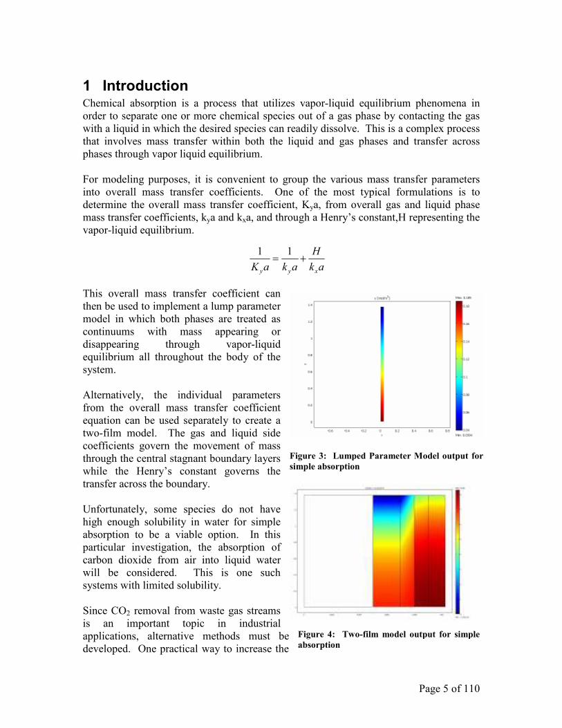
For modeling purposes, it is convenient to group the various mass transfer parameters
into overall mass transfer coefficients. One of the most typical formulations is to
determine the overall mass transfer coefficient, Kya, from overall gas and liquid phase
mass transfer coefficients, kya and kxa, and through a Henry’s constant,H representing the
vapor-liquid equilibrium.
This overall mass transfer coefficient can
then be used to implement a lump parameter
model in which both phases are treated as
continuums with mass appearing or
disappearing through vapor-liquid
equilibrium all throughout the body of the
system.
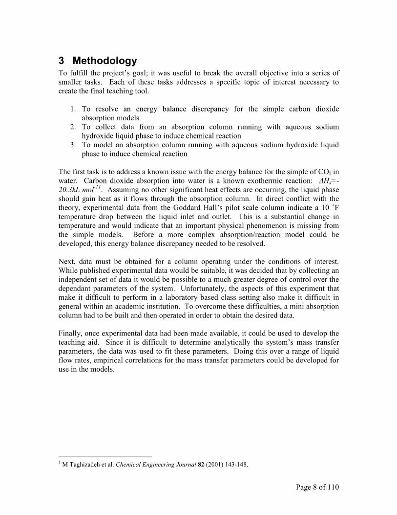
Alternatively, the individual parameters
from the overall mass transfer coefficient
equation can be used separately to create a
two-film model. The gas and liquid side
coefficients govern the movement of mass
through the central stagnant boundary layers
while the Henry’s constant governs the
transfer across the boundary.
Unfortunately, some species do not have
high enough solubility in water for simple
absorption to be a viable option. In this
particular investigation, the absorption of
carbon dioxide from air into liquid water
will be considered. This is one such
systems with limited solubility.
Since CO2 removal from waste gas streams
is an important topic in industrial
applications, alternative methods must be
developed. One practical way to increase the
ak
H
akaK xyy
+=11
Figure 3: Lumped Parameter Model output for
simple absorption
Figure 4: Two-film model output for simple
absorption

Page 6 of 110
removal of CO2 from the gas stream during absorption is to add sodium hydroxide to the
liquid phase. Once the carbon dioxide absorbs, it undergoes reaction with the aqueous
hydroxide ions to form a highly soluble product ion.
Although students study simple absorption during their course of study as chemical
engineers, this enhanced form of absorption is difficult to demonstrate in a class room
setting and is often not included in the curriculum. It would be useful to develop a tool
for studying this type of absorption without the need for physical laboratory equipment.
The remainder of this report represents an effort to fulfill this goal.
OHCOOHCO 2
2
32 2 +→+ −−

Page 7 of 110
2 Objective The objective of this project is to develop an interactive teaching aid that will allow
students to investigate the internal dynamics of an absorption column when it is operated
in conjunction with a liquid phase chemical reaction. Such an aid will allow students to
virtually experiment with this advanced method of absorption without the need to
perform the physical experiment. Since the physical experiments for this type of system
are generally too dangerous and difficult to implement in a laboratory based class setting,
students currently are unable to explore this important process without this teaching aid.
Furthermore, this teaching aid will be developed using COMSOL
Multiphysics software. This program is a powerful finite element package
that combines mesh generation tools, solution solvers, and postprocessing
tools. By establishing a model, students will then be able to enter the
program and adjust specific parameters. By doing this, they can study the
system’s response to various types of variable manipulations.
Page 8 of 110
3 Methodology To fulfill the project’s goal; it was useful to break the overall objective into a series of
smaller tasks. Each of these tasks addresses a specific topic of interest necessary to
create the final teaching tool.
1. To resolve an energy balance discrepancy for the simple carbon dioxide
absorption models
2. To collect data from an absorption column running with aqueous sodium
hydroxide liquid phase to induce chemical reaction
3. To model an absorption column running with aqueous sodium hydroxide liquid
phase to induce chemical reaction
The first task is to address a known issue with the energy balance for the simple of CO2 in
water. Carbon dioxide absorption into water is a known exothermic reaction: ∆Hs=-
20.3kL mol-11. Assuming no other significant heat effects are occurring, the liquid phase
should gain heat as it flows through the absorption column. In direct conflict with the
theory, experimental data from the Goddard Hall’s pilot scale column indicate a 10 ˚F
temperature drop between the liquid inlet and outlet. This is a substantial change in
temperature and would indicate that an important physical phenomenon is missing from
the simple models. Before a more complex absorption/reaction model could be
developed, this energy balance discrepancy needed to be resolved.
Next, data must be obtained for a column operating under the conditions of interest.
While published experimental data would be suitable, it was decided that by collecting an
independent set of data it would be possible to a much greater degree of control over the
dependant parameters of the system. Unfortunately, the aspects of this experiment that
make it difficult to perform in a laboratory based class setting also make it difficult in
general within an academic institution. To overcome these difficulties, a mini absorption
column had to be built and then operated in order to obtain the desired data.
Finally, once experimental data had been made available, it could be used to develop the
teaching aid. Since it is difficult to determine analytically the system’s mass transfer
parameters, the data was used to fit these parameters. Doing this over a range of liquid
flow rates, empirical correlations for the mass transfer parameters could be developed for
use in the models.
1 M Taghizadeh et al. Chemical Engineering Journal 82 (2001) 143-148.
Page 9 of 110
3.1 Resolving the Energy Balance Discrepancy for Simple Absorption Models
The two most likely causes for the decrease in liquid phase temperature across the
column include non isothermal expansion of the gas phase at the base of the column and
heat loss due to evaporation.
As the gas phase enters the column, it emerges from a narrow tube into a much wider
column. This rapid expansion is usually accompanied by a decrease in temperature. If
this heat effect is strong enough, it could be causing the liquid to cool enough to
overcome the heat of absorption.
Alternatively, the liquid phase could be evaporating into the gas phase. The gas used for
these experiments comes from compressed gas cylinders which contain no humidity. As
this dry gas comes in contact with the air some of the liquid will evaporate in order to
humidify the gas until it becomes saturated with water vapor. Since evaporation is an
endothermic process, if sufficient evaporation is occurring, it could overcome the heat of
absorption.
3.1.1 Experiment #1: Non-Isothermal Expansion
3.1.1.1 Objective
To determine the degree of cooling occurring due to isothermal expansion of the gas
phase
3.1.1.2 Equipment
• Goddard Hall Pilot Scale Packed Absorption Tower with peripheral flow controls,
flow meters, and thermo couples
• Compressed air cylinder
• Compressed carbon dioxide cylinder
3.1.1.3 Procedure
For this relatively simple experiment, the column was operated using only a gas phase.
Gas flow rates were adjusted to maintain a constant 1.5 LPM flow of air and 0.3 LPM
flow of carbon dioxide. The system was allowed to run while temperature measurements
were taken at the top and bottom of the column
Page 10 of 110
3.1.2 Experiment #2: Evaporation Heat Loss
3.1.2.1 Objective
To determine if saturating the gas phase with water vapor prior to its use in the column
will prevent the liquid phase temperature drop.
3.1.2.2 Equipment
• Goddard Hall Pilot Scale Packed Absorption Tower with peripheral flow controls,
flow meters, and thermo couples
• Rosemont carbon dioxide analyzer
• Compressed air cylinder
• Compressed carbon dioxide cylinder
• Pressure vessel with appropriate fittings and tubing
• Water
For this experiment, the gas inlet tubes to the column were rerouted. After the junction
where the two gas streams are mixed, the gas was diverted into a pressure vessel. At the
inlet of the vessel, the gas is forced down a vertical, internal tube to emerge at an orifice
located near the bottom of the vessel. A second opening at the top of the pressure vessel
was used as an outlet. Gas emerging from this outlet was then piped into the column.
3.1.2.3 Procedure
To ensure that the water supply to the column remained constant throughout the
experiment, the liquid hold-up tank was first drained of its room temperature water and
then refilled using the buildings water supply which was slightly colder than room
temperature. Thus, as the holding tank refilled during the experiment, it would not
decrease in temperature.
Next the pressure vessel was filled with water from buildings water supply and then
sealed. Once sealed, the gas cylinders were opened and set to flow at cost rates of 1.5
LPM air and 0.3 LPM CO2. With the addition of the pressure vessel, the gasses were
now being bubbled through a water bath before entering the tower. Since the gas would
now be saturated with the water from the tank and not from the flowing water in the
column, there should no longer be a temperature drop across the column.
A liquid flow rate of 1 LPM water was used and measurements were taken over a period
of time once the outlet gas CO2 concentration had reached a steady state.
Page 11 of 110
3.1.3 Experiment #3: Control Case
3.1.3.1 Objective
To analyze the column as it operates under the typical laboratory conditions in order to
determine if some other phenomena may be occurring.
3.1.3.2 Equipment
• Goddard Hall Pilot Scale Packed Absorption Tower with peripheral flow controls,
flow meters, and thermo couples
• Rosemont carbon dioxide analyzer
• Compressed air cylinder
• Compressed carbon dioxide cylinder
• Water
For this experiment, the pressure vessel was left attached to the column; however the
water bath was drained. Effectively, the column set-up as it would be during the
laboratory experiments. The addition of the empty pressure vessel merely increased the
pressure drop over the system without effecting compositions or temperature.
3.1.3.3 Procedure
To ensure that the water supply to the column remained constant throughout the
experiment, the liquid hold-up tank was first drained of its room temperature water and
then refilled using the buildings water supply which was slightly colder than room
temperature. Thus, as the holding tank refilled during the experiment, it would not
decrease in temperature.
The column was then run using a standard set of conditions encountered during a typical
experiment: 1.5 LPM air, 0.3 LPM CO2, and 1.0 LPM water. In addition to recording the
digital readouts from the thermocouples, the temperature of the liquid in the hold up tank
was manually collected using a thermometer.
Page 12 of 110
3.2 Collecting Data from an Absorption/ Reaction System
3.2.1 Obstacles
As previously mentioned, there are many obstacles that must be overcome to run an
absorption with reaction experiment in an academic setting.
First and foremost, the aqueous sodium hydroxide2 to be used as the liquid phase has a
pH of 14. This is extremely hazardous to humans. Contact with the skin, eyes, or lungs
and ingestion can all cause sever burns and scaring. Permanent vision loss, scaring, and
even death can occur if this solution is handled inappropriately. Additionally, pH 14
substances can also be corrosive when they come in contact with inorganic material.
Liquid flowing through the Goddard Hall absorption column comes in contact with a
wide variety of materials including glass packing, gaskets, plastic tubing, metal fittings,
flow meters, and pumps. Any one of these pieces could easily react with the sodium
hydroxide causing permanent damage to the system.
Of lesser concern is the volume of aqueous sodium hydroxide required. The system
requires at least 20 minutes, if not longer, to reach steady state. Even running at the
minimum measurable flow of 0.5 LPM liquid, the volume of liquid required is
substantial. To complicate the matter more, the hold-up tank requires a minimal liquid
level in order to provide net positive suction head (NPSH) to the pump. Therefore a
secondary liquid hold-up tank would need to be designed in order to gravity feed the first
hold-up tank and maintain NPSH.
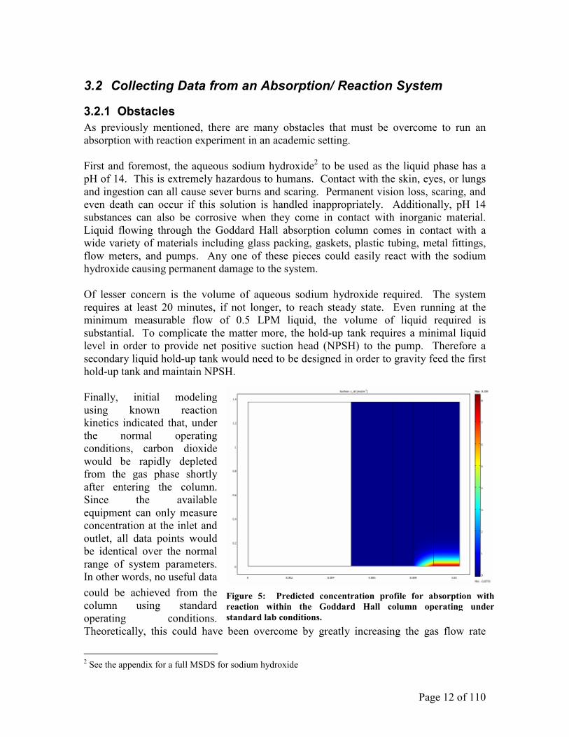
Finally, initial modeling
using known reaction
kinetics indicated that, under
the normal operating
conditions, carbon dioxide
would be rapidly depleted
from the gas phase shortly
after entering the column.
Since the available
equipment can only measure
concentration at the inlet and
outlet, all data points would
be identical over the normal
range of system parameters.
In other words, no useful data
could be achieved from the
column using standard
operating conditions.
Theoretically, this could have been overcome by greatly increasing the gas flow rate
2 See the appendix for a full MSDS for sodium hydroxide
Figure 5: Predicted concentration profile for absorption with reaction within the Goddard Hall column operating under
standard lab conditions.
Page 13 of 110
while decreasing the liquid flow—essentially contacting more CO2 with less liquid in
hopes of some of the CO2 remaining at the outlet. However, this method has its own
inherent issue. The flow meters on the system would have to be replaced since the
current meters would not be sensitive enough to fine tune the liquid flow rate and the
high gas flows would physically damage the gas flow meters.
Overall, among the safety issues for humans and equipment, the high volume of solution
required, and the inability to obtain usable data, it became apparent that using the
Goddard Hall pilot scale column would be completely impractical. Instead, it was
decided to create a miniature absorption column that could be operated under more
favorable conditions. Although the safety issues still remained, this new approach
negated the latter two concerns.
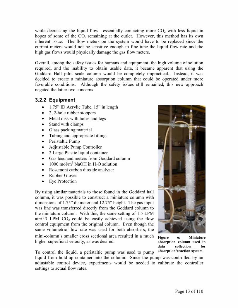
3.2.2 Equipment
• 1.75” ID Acrylic Tube, 15” in length
• 2, 2-hole rubber stoppers
• Metal disk with holes and legs
• Stand with clamps
• Glass packing material
• Tubing and appropriate fittings
• Peristaltic Pump
• Adjustable Pump Controller
• 2 Large Plastic liquid container
• Gas feed and meters from Goddard column
• 1000 mol/m3 NaOH in H2O solution
• Rosemont carbon dioxide analyzer
• Rubber Gloves
• Eye Protection
By using similar materials to those found in the Goddard hall
column, it was possible to construct a miniature column with
dimensions of 1.75” diameter and 12.75” height. The gas input
was line was transferred directly from the Goddard column to
the miniature column. With this, the same setting of 1.5 LPM
air/0.3 LPM CO2 could be easily achieved using the flow
control equipment from the original column. Even though the
same volumetric flow rate was used for both absorbers, the
mini-column’s smaller cross sectional area resulted in a much
higher superficial velocity, as was desired.
To control the liquid, a peristaltic pump was used to pump
liquid from hold-up container into the column. Since the pump was controlled by an
adjustable control device, experiments would be needed to calibrate the controller
settings to actual flow rates.
Figure 6: Miniature absorption column used in
data collection for
absorption/reaction system

Page 14 of 110
3.2.3 Experiment #4: Liquid Flow Rates
3.2.3.1 Objective
To correlate the adjustable controller’s
settings to the actual liquid flow rates.
3.2.3.2 Equipment
• Peristaltic Pump
• Adjustable Pump Controller
• Tubing
• Stop Watch
• 250 mL graduated cylinder
3.2.3.3 Procedure
Setting the controller to an incremental value between 2 and 6 inclusive, the pump output
was collected in the graduated cylinder for a fixed period of time. Thus the liquid
volumetric flow rate could be determined. Unfortunately, the controller was continuous
and could be set at any position between two intervals. This allowed for the possibility
that each time it was set to a specific number, it may have been slightly different than the
previous time. Since nothing could be done about this flaw, the small amount of error
that it introduced will have to be acceptable.
3.2.4 Experiment #5: Simple Absorption in Mini-Column
3.2.4.1 Objective
To obtain data for simple absorption in the mini-column that can be used to determine
fitted overall mass transfer coefficients.
3.2.4.2 Equipment
• Miniature column and pump assembly
• Rosemont carbon dioxide analyzer
• Air and carbon dioxide
• Distilled water
3.2.4.3 Procedure
The column was run with a fixed gas flow rate of 1.5 LPM air/ 0.3 LPM CO2. Liquid
flow rate was adjusted from setting 2 to setting 6 (0.136 to 0.4 L/min). At each liquid
flow, the column was allowed to run until exiting gas phase CO2 concentration reached
steady state for at least 1 minute. Liquid output was captured in a plastic jar and disposed
of after the experiment.
Figure 7: Adjustable Control on Pump Control Device

Page 15 of 110
3.2.5 Experiment #6: Absorption/Reaction in Mini-Column
3.2.5.1 Objective
To obtain data for absorption/reaction in the mini-column that can be used to develop the
absorption/reaction model.
3.2.5.2 Equipment
• Miniature column and pump assembly
• Rosemont carbon dioxide analyzer
• Air and carbon dioxide
• 1000 mol/m3 NaOH solution
3.2.5.3 Procedure
NaOH solution was prepared by adding 40 grams of NaOH pellet per liter of water.
Pellets were slowly dissolved into a portion of the water using a stirring rod. The final
solution was then diluted to the proper volume. NaOH solution sat at room temperature
for an hour before experiments were performed.
The column was run with a fixed gas flow rate of 1.5 LPM air/ 0.3 LPM CO2. Liquid
flow rate was adjusted from setting 2 to setting 6 (0.136 to 0.4 L/min). At each liquid
flow, the column was allowed to run until exiting gas phase CO2 concentration reached
steady state for at least 1 minute. Liquid output was captured in a plastic jar and disposed
of after the experiment.
3.2.5.4 Safety
Latex gloves and safety glasses were worn at all times when handling NaOH. NaOH
container was clearly labeled and stored on sturdy surfaces. Unnecessary personal were
asked to keep their distance from the equipment during operation.
Waste NaOH was first diluted before flushing down a chemical drain. Equipment was
thoroughly and repeatedly rinsed with fresh water. Solid material found trapped in
chemical drain was thoroughly washed and disposed of in appropriate receptacle. pH
tests were performed on all equipment pieces to ensure pH neutrality before leaving the
laboratory.
Page 16 of 110
3.3 Modeling Absorption/ Reaction System
3.3.1 Overall Mass Transfer Coefficient
For the lumped parameter model, two differential equations are used: one for the liquid
phase and on for the gas phase CO2.
cuRcD ∇⋅−=∇−⋅∇ )(
Using known diffusivities for carbon dioxide in water and air3 and the experimentally set
flow rates, the only remaining parameter is the reaction term R. In the liquid phase
)( *yyaKR y −⋅=
representing an overall transfer of mass into the liquid phase. Simultaneously, this mass
must be removed from the gas phase, so
)( *yyaKR y −⋅−=
Determining y* by means of Henry’s Law, the overall mass transfer coefficient, Kya is the
only tunable parameter in the lumped model. Setting the correct inlet concentrations, the
Kya parameter can then be adjusted for each flow rate in order to find a the value that will
yield the correct outlet concentration. In this way an empirical correlation can be
determined to find the overall mass transfer coefficient given various liquid flow rates.
3.3.2 Gas Phase Mass Transfer Coefficient
By modifying the lumped parameter model slightly, it can be easily adapted to
incorporate a liquid phase chemical reaction. In fact, in terms of the CO2 balances, the
only change needed is to add a consumption term to R:
−−−⋅=OHCOby CCkyyaKR
2)( *
The only complication is that additional mass balances must also be added to track not
only the OH- concentration, but also the Na
+ and CO3
2- concentrations since the reaction
rate constant is dependant on these ionic concentrations. From the literature4, an
empirical correlation can be found for this constant:
2016.0221.0/2382895.11)log( IITkb −+−=
Where “I” is the ionic strength of the solution and T can be taken as room temperature.
3 Clark, W. M. “COMSOL Multiphysics Models for Teaching Chemical Engineering Fundamentals:
Absorption Column Models and Illustration of the Two-Film Theory of Mass Transfer.” 2008. 4 M. Taghizadeh et al. Chemical Engineering Journal 82 (2001) 143-148
Page 17 of 110
After making these modifications to the model, it was seen that very little reaction was
occurring, indicating an error in the model. It was soon realized that, by using the overall
mass transfer coefficient from a system without reaction, the model was artificially
imposing a liquid phase mass transfer resistance. Since the reaction had been added
specifically to remove this barrier to mass transfer, it is wrong to use the overall mass
transfer coefficient. Instead, only gas phase mass transfer coefficient should impact the
system.
y
yxyy
Hakak
H
akaK=≅+=
111
Once again, but adjusting the mass transfer coefficient, a correlation can be developed
between liquid flow rate and overall gas phase mass transfer coefficient, kya. The
validity of this equation can be tested by comparing the results to known correlations5:
5.035.05.05.0
782.6678.0782.6660.0
226.0−−
=
= xyx
p
y
GC
GGSc
fH
Here fp is an unknown packing parameter, Sc is the Schmidt number, and Gx and Gy are
liquid and gas phase superficial velocities respectively. Since everything except the
liquid phase superficial velocity is constant for these experiments, it can be seen that a
correlation to the gas phase mass transfer resistance, Hy, should be directly proportional
by some constant C, to Gx raised to the inverse, one-half power.
3.3.3 Two-Film Absorption with Reaction Model
Using known rate constant, diffusivities, and Henry’s constant in addition to the
empirical correlations for mass transfer coefficients, the two-film model is easily adapted
to reflect absorption with chemical reaction. The correlation for the overall gas phase
mass transfer coefficient is used directly in the model to predict the CO2 behavior in the
stagnant gas film. Within the stagnant liquid film, the overall mass transfer coefficient is
set to an arbitrarily large value to ensure that the liquid phase resistance to mass transfer
is close to zero. Finally, reaction terms are added to both the stagnant liquid film and the
falling liquid layer in order to account for the removal of CO2 by chemical reaction. As
with the lumped parameter model, extra differential equations were added to track the
liquid phase ion concentrations.
5 Geankoplis. Transport Processes and Separation Process Principles. Prentice Hall: Upper Saddle River,
NJ, 2003

Page 18 of 110
Top Bottom
77 73
77 71
77 65
Table 1: Temperature
data (˚F) collected at
intervals over a 45
minute period
Top Bottom
68 55
67 55
Table 2: Temperature
data (˚F) for column
with preconditioned gas phase
Top Bottom
72 74
72 66
70 58
70 58
69 57
Table 3: Temperature
data (˚F) for column
under standard conditions
4 Results
4.1 Resolved the Energy Balance Discrepancy for Simple Absorption Models
4.1.1 Experiment #1: Non-Isothermal Expansion
After a period of about 45 minutes, the bottom of the column was
approximately 12 ˚F cooler than the top of the column. This
suggests that there is in fact cooling occurring due to the non-
isothermal expansion of the gas phase.
However, this similarity in temperature drop does not correspond
to an equivalent heat loss. The heat capacity of air in this
temperature range is approximately 1.00 kJ/kg*K while the heat
capacity of water is approximately 4.18 kJ/kg*K6. Taking into consideration the density
of air and water (1.17 kg/m^3 and 1000 kg/m^3 respectively)7, a 12˚F temperature drop
in the gas would correspond to the gas absorbing 7.8 kJ/m^3 of heat. For the liquid to
supply this heat, its temperature would only fall by 0.003 ˚F.
Clearly, non-isothermal expansion is not responsible for the temperature drop across the
column. While this experiment demonstrated that there was indeed cooling due to this
phenomena, it is so insignificant that it can be neglected from the overall model without
incurring significant error
4.1.2 Experiment #2: Evaporation Heat Loss
After allowing the column to approach steady state, there was a
12˚F temperature drop over the column despite the addition of the
humidification system. This indicates that while there may be
evaporation and cooling occurring within the standard system, it is
not causing the overall discrepancy with the energy balance.
4.1.3 Experiment #3: Control Case
By performing the experiment under the standard conditions, it
was possible to reproduce the 12˚F temperature drop across the
column. However, measurement of the water in the liquid hold-up
tank showed it to be approximately 54.5˚F. This is significantly
cooler than the temperature at the top of the column. While the
liquid pump does add a small amount of heat to the liquid to get it
to the top of the column, it does not add 15˚F. It is therefore likely
that the temperature of the water at the top of the column is
actually closer to 55 or 56˚F.
6 Incropera, Dewitt, Bergman, and Lavine. Introduction to Heat Transfer. 5
th ed. John Wiley & Sons:
USA, 2007. 7 ibid

Page 19 of 110
Table 4: Flow rate vs.
Controller Setting
Setting W(L/min)
off 0
2 0.136
3 0.23
4 0.284
5 0.348
6 0.4
Likely, the thermocouple at the top of the column is either inappropriately positioned or
malfunctioning. If the top thermocouple is not adequately contacting the liquid phase
then it will not give an accurate reading of the liquid phase temperature. To correct this,
the thermocouple would need to be placed either directly under the liquid phase inlet so
that the liquid would fully coat the thermocouple or the thermocouple should be placed
within the liquid phase input pipe. Alternatively, if the thermocouple is accurately
placed, it could just be malfunctioning and needing replacement.
In light of these results, it can be seen that there actually is not a discrepancy in the
energy balance. The system is consistent with the theory being applied. It was merely an
in appropriately interpreted temperature reading that was causing confusion.
As an unexpected result, the new data showed that system was only experiencing a
temperature increase of less than 1 or 2˚F. Since the mass transfer parameters are not
highly sensitive to temperature changes, this experiment showed that it was not necessary
to include the energy balance in the teaching aid. This will significantly reduce the
complexity of the tool, making it easier for students to understand.
4.2 Collecting Data from an Absorption/ Reaction System
4.2.1 Experiment #4: Liquid Flow Rates
By collecting the output for 30sec or 1 min at each setting, it
was possible to generate a table correlating the controller settings
to actual liquid flow rates. As expected, the flow rate increases
with increase setting, but it is not a linear relationship: Flow
increases slower as setting increase. Again this could have some
error due to the inability to set the controller in exactly the same
spot each time. Also, as the tubing inside the pump began to
physically deteriorate due to the stresses, it could have affected
the flow rate.

Page 20 of 110
4.2.2 Experiments # 5 & #6: Simple Absorption and Absorption/Reaction Data Collection
Both experiments produced well behaved data sets. Both appropriately exhibited
decreasing linear trends. As expected, the simply absorption experiment showed poor
removal of CO2 from the gas stream. With an inlet concentration of 17.5 mol-%, the
highest water flow rate only decreased the CO2 by 1.4 mol-%. The absorption with
reaction system, in comparison, performed exceedingly well decreasing the CO2 mole
fraction by as much as 17.5 mol-% from 17.8 mol-% at the inlet to under 3 mol-% at the
outlet. Both sets of data are meaningful and will be useful in developing the model.
0.16
0.161
0.162
0.163
0.164
0.165
0.166
0.167
0.168
0.169
0.1 0.15 0.2 0.25 0.3 0.35 0.4 0.45
Volumetric Liquid Flow Rate (L/min)
Ga
s O
utl
et
Mo
le F
rac
tio
n (
no
rea
cti
on
)
0
0.01
0.02
0.03
0.04
0.05
0.06
0.07
Ga
s O
utl
et
Mo
le F
rac
tio
n (
wit
h r
xn
)
Figure 8: Output concentration versus volumetric liquid flow rate for simple absorption (blue) and
absorption with reaction (red).
During both experiments, it was qualitatively determined that heat effects were minimal
within the absorption column. This indicated that a detailed energy balance could be
neglected from the final teaching aid in order keep it as easy to understand as possible.
Page 21 of 110
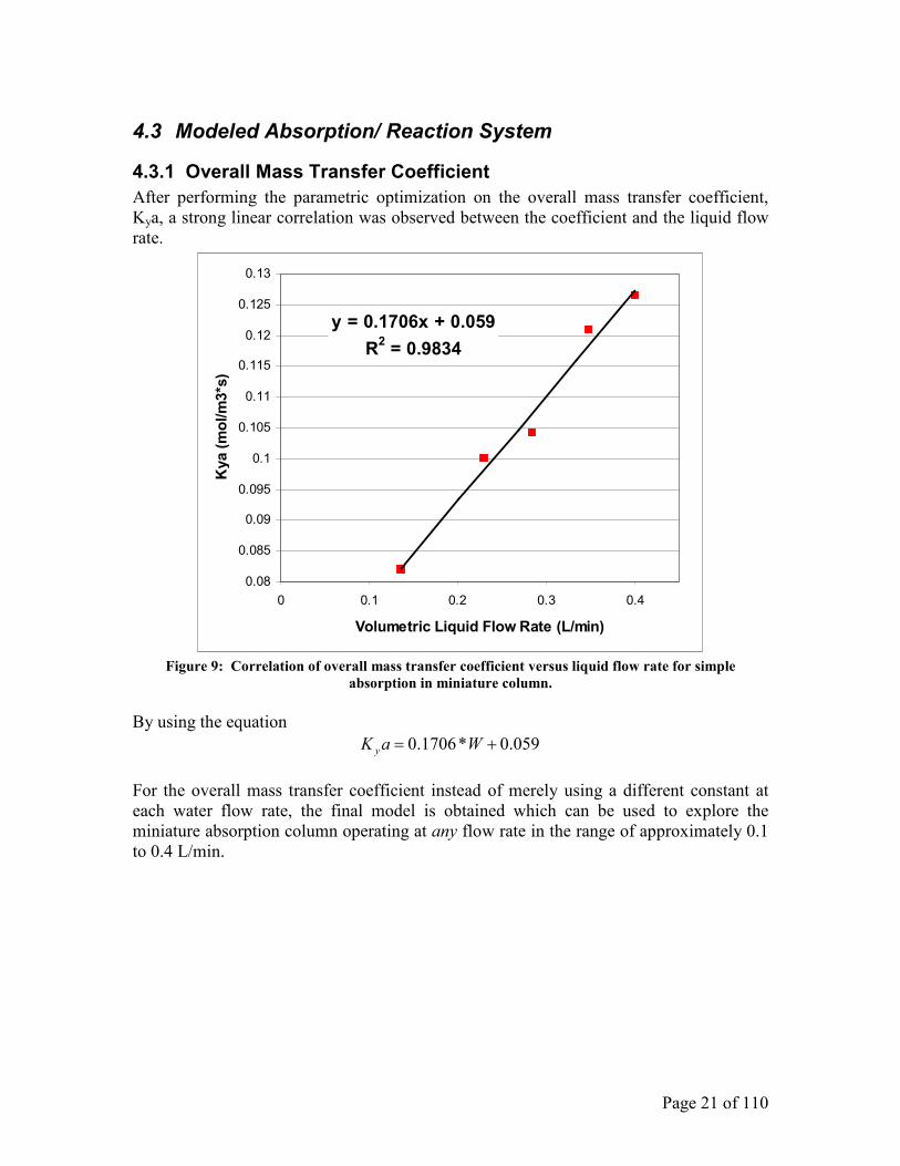
4.3 Modeled Absorption/ Reaction System
4.3.1 Overall Mass Transfer Coefficient
After performing the parametric optimization on the overall mass transfer coefficient,
Kya, a strong linear correlation was observed between the coefficient and the liquid flow
rate.
y = 0.1706x + 0.059
R2 = 0.9834
0.08
0.085
0.09
0.095
0.1
0.105
0.11
0.115
0.12
0.125
0.13
0 0.1 0.2 0.3 0.4
Volumetric Liquid Flow Rate (L/min)
Kya (
mo
l/m
3*s
)
Figure 9: Correlation of overall mass transfer coefficient versus liquid flow rate for simple
absorption in miniature column.
By using the equation
059.0*1706.0 += WaK y
For the overall mass transfer coefficient instead of merely using a different constant at
each water flow rate, the final model is obtained which can be used to explore the
miniature absorption column operating at any flow rate in the range of approximately 0.1
to 0.4 L/min.

Page 22 of 110
Figure 10: Estimated gas phase concentration profile for column operating at 0.3 L/min liquid flow
rate
4.3.2 Gas Phase Mass Transfer Coefficient
Using the above obtained mass transfer coefficient with known kinetics data, it was
quickly seen that the overall mass transfer coefficient was not the appropriate way to
model the system undergoing reaction.
Table 5: Calculated and Experimental Outlet concentrations for absorption/reaction system.
Liquid Flow
(L/min)
Y Out,
Experimental
Y Out,
Calculated
Y Out,
No Rxn
0.23 0.05 0.165 0.165
0.284 0.037 0.163 0.164
0.348 0.031 0.162 0.162
0.4 0.027 0.161 0.161
By using the overall mass transfer coefficient that includes liquid phase mass transfer
resistance, almost no CO2 is able to react within the liquid phase causing the model to
predict results nearly identical to the experimental data for the simple absorption system.
A better approach is to assume no liquid phase transfer resistance and to use the
experimental data to find a second correlation for the overall mass transfer coefficient.
Page 23 of 110
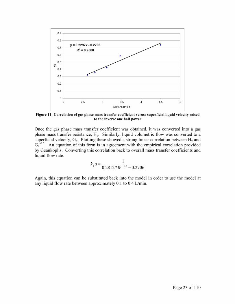
y = 0.2297x - 0.2706
R2 = 0.9568
0
0.1
0.2
0.3
0.4
0.5
0.6
0.7
0.8
0.9
2 2.5 3 3.5 4 4.5 5
(Gx/6.782)^-0.5
Hy
Figure 11: Correlation of gas phase mass transfer coefficient veruss superficial liquid velocity raised
to the inverse one half power
Once the gas phase mass transfer coefficient was obtained, it was converted into a gas
phase mass transfer resistance, Hy. Similarly, liquid volumetric flow was converted to a
superficial velocity, Gx. Plotting these showed a strong linear correlation between Hy and
Gx-0.5
. An equation of this form is in agreement with the empirical correlation provided
by Geankoplis. Converting this correlation back to overall mass transfer coefficients and
liquid flow rate:
2706.0*2812.0
15.0 −
=−W
ak y
Again, this equation can be substituted back into the model in order to use the model at
any liquid flow rate between approximately 0.1 to 0.4 L/min.
Page 24 of 110
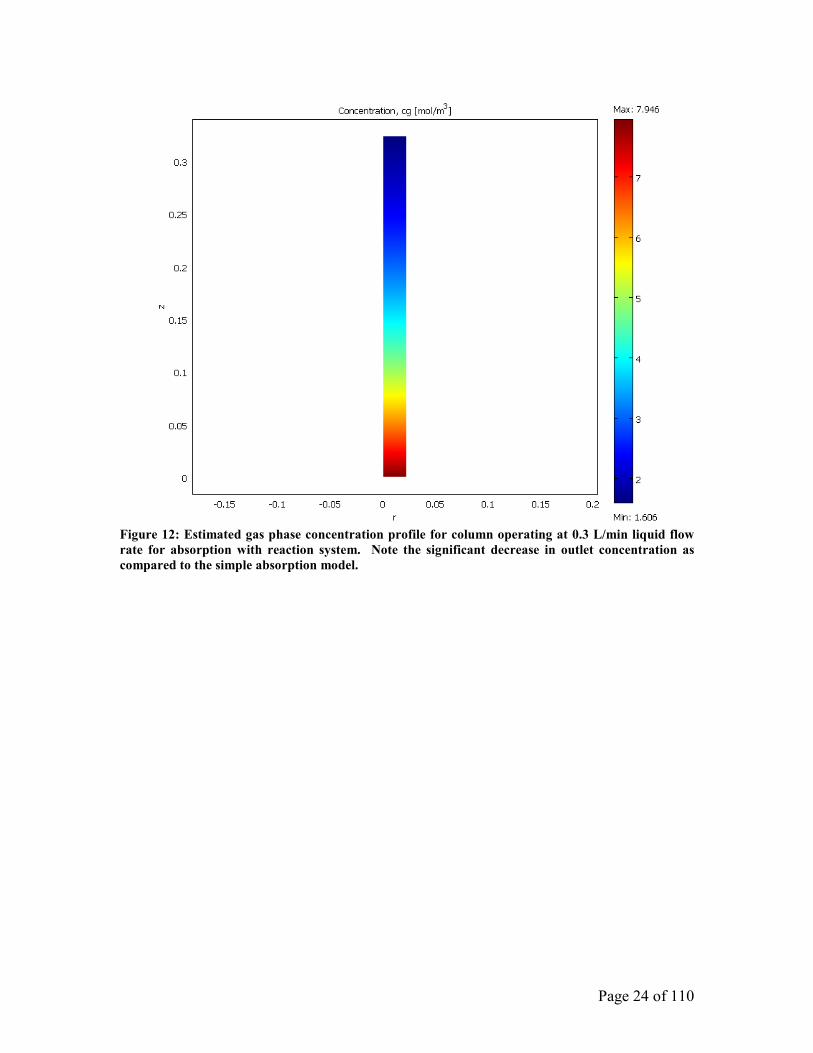
Figure 12: Estimated gas phase concentration profile for column operating at 0.3 L/min liquid flow
rate for absorption with reaction system. Note the significant decrease in outlet concentration as
compared to the simple absorption model.
Page 25 of 110
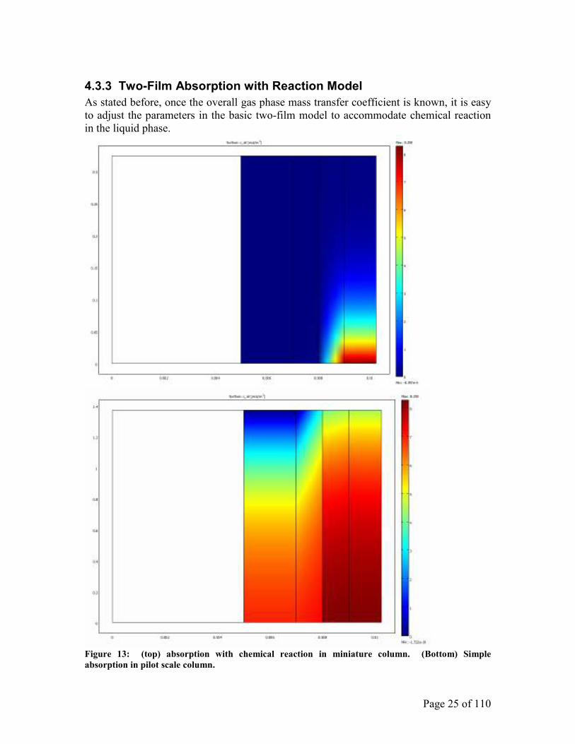
4.3.3 Two-Film Absorption with Reaction Model
As stated before, once the overall gas phase mass transfer coefficient is known, it is easy
to adjust the parameters in the basic two-film model to accommodate chemical reaction
in the liquid phase.
Figure 13: (top) absorption with chemical reaction in miniature column. (Bottom) Simple
absorption in pilot scale column.
Page 26 of 110
The resulting model over predicts the amount of CO2 being removed from the liquid
phase. In fact, all of the CO2 is removed within the column for all flow rates in the range
0.1 to 0.4 L/min. This error could a result of any number of the small experimental errors
and theoretical simplifications that have been during the development of this model.
What is important to see is that the drastic differences between this new model and a
simple absorption model. When these two models are compared, it is very easy to
understand the effects of adding the liquid phase chemical reaction. Predominately,
without reaction, the liquid phase is quickly saturated with carbon dioxide. Once
chemical reaction is added, practically no dissolved CO2 is present. It has all been
converted into CO32-. As a result of this rapid removal from the liquid phase,
significantly greater quantities of the CO2 can be removed from the gas phase.
Therefore, although the new model is not 100% accurate in comparison to experimental
data, it simulates the appropriate behavior and will make a useful tool for students trying
to explore this advanced form of absorption.
Page 27 of 110
5 Conclusions After reexamining the pilot scale absorption column, it was determined that heat effects
within the system were negligible. The apparent discrepancy with the energy balance
was simply a result of thermocouple error. This determination allowed for the models to
be simplified by excluding energy balances. Although a full analysis of the system
would in fact include an energy balance, this would only add unnecessary complexity to
the teaching aid when its purpose is to show the difference of adding a chemical reaction
and not the weak temperature effects.
For the actual teaching aid, a decent set of experimental data was collected using a
miniature absorption column. This data was then analyzed to determine fitted parameters
for the absorption models. The resulting two-film model had a small degree of error, but
was sufficiently accurate to successfully demonstrate the advantages of using chemical
reaction in combination with absorption. Although the current model is limited to only
varying the liquid flow rate, this does not limit the models value. In fact, in industrial
settings, the gas stream that must be cleaned of contaminates is typically provided at a
fixed rate. Thus the engineering only has access to the liquid flow rate and the column
dimensions in order to achieve the desired purification of the gas stream.
In the future, several tasks could be performed to possibly improve the accuracy and
flexibility of the model. First, repetition of the experimental results could confirm their
accuracy. Then, by changing the gas flow rates, the model could be modified to account
for both a variable liquid and gas rate instead of just a variable liquid rate. Finally, it is
possible that there is, in fact, a small amount of liquid phase resistance to mass transfer.
By adding in this small resistance, it is possible that the appropriate output compositions
would be achieved for the system. Additional experiments and literature review would
be necessary to investigate this possibility.
Page 28 of 110
6 References Clark, W. M. “COMSOL Multiphysics Models for Teaching Chemical Engineering
Fundamentals: Absorption Column Models and Illustration of the Two-Film
Theory of Mass Transfer.” 2008.
Geankoplis. Transport Processes and Separation Process Principles. Prentice Hall:
Upper Saddle River, NJ, 2003
Incropera, Dewitt, Bergman, and Lavine. Introduction to Heat Transfer. 5th ed. John
Wiley & Sons: USA, 2007.
M Taghizadeh et al. Chemical Engineering Journal 82 (2001) 143-148.
Page 29 of 110
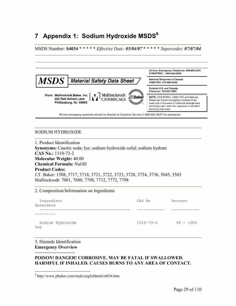
7 Appendix 1: Sodium Hydroxide MSDS8
MSDS Number: S4034 * * * * * Effective Date: 05/04/07 * * * * * Supercedes: 07/07/04
SODIUM HYDROXIDE
1. Product Identification
Synonyms: Caustic soda; lye; sodium hydroxide solid; sodium hydrate
CAS No.: 1310-73-2
Molecular Weight: 40.00
Chemical Formula: NaOH
Product Codes: J.T. Baker: 1508, 3717, 3718, 3721, 3722, 3723, 3728, 3734, 3736, 5045, 5565
Mallinckrodt: 7001, 7680, 7708, 7712, 7772, 7798
2. Composition/Information on Ingredients
Ingredient CAS No Percent
Hazardous
--------------------------------------- ------------ ------------
---------
Sodium Hydroxide 1310-73-2 99 - 100%
Yes
3. Hazards Identification
Emergency Overview --------------------------
POISON! DANGER! CORROSIVE. MAY BE FATAL IF SWALLOWED.
HARMFUL IF INHALED. CAUSES BURNS TO ANY AREA OF CONTACT.
8 http://www.jtbaker.com/msds/englishhtml/s4034.htm
Page 30 of 110
REACTS WITH WATER, ACIDS AND OTHER MATERIALS.
SAF-T-DATA(tm)
Ratings (Provided here for your convenience)
-----------------------------------------------------------------------------------------------------------
Health Rating: 4 - Extreme (Poison)
Flammability Rating: 0 - None
Reactivity Rating: 2 - Moderate
Contact Rating: 4 - Extreme (Corrosive)
Lab Protective Equip: GOGGLES & SHIELD; LAB COAT & APRON; VENT HOOD;
PROPER GLOVES
Storage Color Code: White Stripe (Store Separately)
-----------------------------------------------------------------------------------------------------------
Potential Health Effects ----------------------------------
Inhalation: Severe irritant. Effects from inhalation of dust or mist vary from mild irritation to serious
damage of the upper respiratory tract, depending on severity of exposure. Symptoms may
include sneezing, sore throat or runny nose. Severe pneumonitis may occur.
Ingestion: Corrosive! Swallowing may cause severe burns of mouth, throat, and stomach. Severe
scarring of tissue and death may result. Symptoms may include bleeding, vomiting,
diarrhea, fall in blood pressure. Damage may appear days after exposure.
Skin Contact: Corrosive! Contact with skin can cause irritation or severe burns and scarring with
greater exposures.
Eye Contact: Corrosive! Causes irritation of eyes, and with greater exposures it can cause burns that
may result in permanent impairment of vision, even blindness.
Chronic Exposure: Prolonged contact with dilute solutions or dust has a destructive effect upon tissue.
Aggravation of Pre-existing Conditions: Persons with pre-existing skin disorders or eye problems or impaired respiratory function
may be more susceptible to the effects of the substance.
4. First Aid Measures
Inhalation: Remove to fresh air. If not breathing, give artificial respiration. If breathing is difficult,
give oxygen. Call a physician.
Ingestion: DO NOT INDUCE VOMITING! Give large quantities of water or milk if available.
Never give anything by mouth to an unconscious person. Get medical attention
immediately.
Skin Contact: Immediately flush skin with plenty of water for at least 15 minutes while removing
Page 31 of 110
contaminated clothing and shoes. Call a physician, immediately. Wash clothing before
reuse.
Eye Contact: Immediately flush eyes with plenty of water for at least 15 minutes, lifting lower and
upper eyelids occasionally. Get medical attention immediately.
Note to Physician: Perform endoscopy in all cases of suspected sodium hydroxide ingestion. In cases of
severe esophageal corrosion, the use of therapeutic doses of steroids should be
considered. General supportive measures with continual monitoring of gas exchange,
acid-base balance, electrolytes, and fluid intake are also required.
5. Fire Fighting Measures
Fire: Not considered to be a fire hazard. Hot or molten material can react violently with water.
Can react with certain metals, such as aluminum, to generate flammable hydrogen gas.
Explosion: Not considered to be an explosion hazard.
Fire Extinguishing Media: Use any means suitable for extinguishing surrounding fire. Adding water to caustic
solution generates large amounts of heat.
Special Information: In the event of a fire, wear full protective clothing and NIOSH-approved self-contained
breathing apparatus with full facepiece operated in the pressure demand or other positive
pressure mode.
6. Accidental Release Measures
Ventilate area of leak or spill. Keep unnecessary and unprotected people away from area
of spill. Wear appropriate personal protective equipment as specified in Section 8. Spills:
Pick up and place in a suitable container for reclamation or disposal, using a method that
does not generate dust. Do not flush caustic residues to the sewer. Residues from spills
can be diluted with water, neutralized with dilute acid such as acetic, hydrochloric or
sulfuric. Absorb neutralized caustic residue on clay, vermiculite or other inert substance
and package in a suitable container for disposal.
US Regulations (CERCLA) require reporting spills and releases to soil, water and air in
excess of reportable quantities. The toll free number for the US Coast Guard National
Response Center is (800) 424-8802.
7. Handling and Storage
Keep in a tightly closed container. Protect from physical damage. Store in a cool, dry,
ventilated area away from sources of heat, moisture and incompatibilities. Always add
the caustic to water while stirring; never the reverse. Containers of this material may be
hazardous when empty since they retain product residues (dust, solids); observe all
warnings and precautions listed for the product. Do not store with aluminum or
magnesium. Do not mix with acids or organic materials.

Page 32 of 110
8. Exposure Controls/Personal Protection
Airborne Exposure Limits: - OSHA Permissible Exposure Limit (PEL):
2 mg/m3 Ceiling
- ACGIH Threshold Limit Value (TLV):
2 mg/m3 Ceiling
Ventilation System: A system of local and/or general exhaust is recommended to keep employee exposures
below the Airborne Exposure Limits. Local exhaust ventilation is generally preferred
because it can control the emissions of the contaminant at its source, preventing
dispersion of it into the general work area. Please refer to the ACGIH document,
Industrial Ventilation, A Manual of Recommended Practices, most recent edition, for
details.
Personal Respirators (NIOSH Approved): If the exposure limit is exceeded and engineering controls are not feasible, a half
facepiece particulate respirator (NIOSH type N95 or better filters) may be worn for up to
ten times the exposure limit or the maximum use concentration specified by the
appropriate regulatory agency or respirator supplier, whichever is lowest.. A full-face
piece particulate respirator (NIOSH type N100 filters) may be worn up to 50 times the
exposure limit, or the maximum use concentration specified by the appropriate regulatory
agency, or respirator supplier, whichever is lowest. If oil particles (e.g. lubricants, cutting
fluids, glycerine, etc.) are present, use a NIOSH type R or P filter. For emergencies or
instances where the exposure levels are not known, use a full-facepiece positive-pressure,
air-supplied respirator. WARNING: Air-purifying respirators do not protect workers in
oxygen-deficient atmospheres.
Skin Protection: Wear impervious protective clothing, including boots, gloves, lab coat, apron or
coveralls, as appropriate, to prevent skin contact.
Eye Protection: Use chemical safety goggles and/or a full face shield where splashing is possible.
Maintain eye wash fountain and quick-drench facilities in work area.
9. Physical and Chemical Properties
Appearance: White, deliquescent pellets or flakes.
Odor: Odorless.
Solubility: 111 g/100 g of water.
Specific Gravity: 2.13
pH: 13 - 14 (0.5% soln.)
% Volatiles by volume @ 21C (70F): 0

Page 33 of 110
Boiling Point: 1390C (2534F)
Melting Point: 318C (604F)
Vapor Density (Air=1): > 1.0
Vapor Pressure (mm Hg): Negligible.
Evaporation Rate (BuAc=1): No information found.
10. Stability and Reactivity
Stability: Stable under ordinary conditions of use and storage. Very hygroscopic. Can slowly pick
up moisture from air and react with carbon dioxide from air to form sodium carbonate.
Hazardous Decomposition Products: Sodium oxide. Decomposition by reaction with certain metals releases flammable and
explosive hydrogen gas.
Hazardous Polymerization: Will not occur.
Incompatibilities: Sodium hydroxide in contact with acids and organic halogen compounds, especially
trichloroethylene, may causes violent reactions. Contact with nitromethane and other
similar nitro compounds causes formation of shock-sensitive salts. Contact with metals
such as aluminum, magnesium, tin, and zinc cause formation of flammable hydrogen gas.
Sodium hydroxide, even in fairly dilute solution, reacts readily with various sugars to
produce carbon monoxide. Precautions should be taken including monitoring the tank
atmosphere for carbon monoxide to ensure safety of personnel before vessel entry.
Conditions to Avoid: Moisture, dusting and incompatibles.
11. Toxicological Information
Irritation data: skin, rabbit: 500 mg/24H severe; eye rabbit: 50 ug/24H severe;
investigated as a mutagen. --------\Cancer Lists\-----------------------------------------------
-------
---NTP Carcinogen---
Ingredient Known Anticipated IARC
Category
------------------------------------ ----- ----------- ------
-------
Sodium Hydroxide (1310-73-2) No No
None
12. Ecological Information
Environmental Fate: No information found.
Page 34 of 110
Environmental Toxicity: No information found.
13. Disposal Considerations
Whatever cannot be saved for recovery or recycling should be handled as hazardous
waste and sent to a RCRA approved waste facility. Processing, use or contamination of
this product may change the waste management options. State and local disposal
regulations may differ from federal disposal regulations. Dispose of container and unused
contents in accordance with federal, state and local requirements.
14. Transport Information
Domestic (Land, D.O.T.) -----------------------
Proper Shipping Name: SODIUM HYDROXIDE, SOLID
Hazard Class: 8
UN/NA: UN1823
Packing Group: II
Information reported for product/size: 300LB
International (Water, I.M.O.) -----------------------------
Proper Shipping Name: SODIUM HYDROXIDE, SOLID
Hazard Class: 8
UN/NA: UN1823
Packing Group: II
Information reported for product/size: 300LB
15. Regulatory Information --------\Chemical Inventory Status - Part 1\-------------------------
--------
Ingredient TSCA EC Japan
Australia
----------------------------------------------- ---- --- ----- --
-------
Sodium Hydroxide (1310-73-2) Yes Yes Yes
Yes
--------\Chemical Inventory Status - Part 2\-------------------------
--------
--Canada--
Ingredient Korea DSL NDSL
Phil.
----------------------------------------------- ----- --- ---- -
----
Sodium Hydroxide (1310-73-2) Yes Yes No
Yes
--------\Federal, State & International Regulations - Part 1\--------
--------
Page 35 of 110
-SARA 302- ------SARA
313------
Ingredient RQ TPQ List
Chemical Catg.
----------------------------------------- --- ----- ---- ------
--------
Sodium Hydroxide (1310-73-2) No No No
No
--------\Federal, State & International Regulations - Part 2\--------
--------
-RCRA- -
TSCA-
Ingredient CERCLA 261.33 8(d)
----------------------------------------- ------ ------ -----
-
Sodium Hydroxide (1310-73-2) 1000 No No
Chemical Weapons Convention: No TSCA 12(b): No CDTA: No
SARA 311/312: Acute: Yes Chronic: No Fire: No Pressure: No
Reactivity: Yes (Pure / Solid)
Australian Hazchem Code: 2R
Poison Schedule: S6
WHMIS: This MSDS has been prepared according to the hazard criteria of the Controlled Products
Regulations (CPR) and the MSDS contains all of the information required by the CPR.
16. Other Information
NFPA Ratings: Health: 3 Flammability: 0 Reactivity: 1
Label Hazard Warning: POISON! DANGER! CORROSIVE. MAY BE FATAL IF SWALLOWED. HARMFUL
IF INHALED. CAUSES BURNS TO ANY AREA OF CONTACT. REACTS WITH
WATER, ACIDS AND OTHER MATERIALS.
Label Precautions: Do not get in eyes, on skin, or on clothing.
Do not breathe dust.
Keep container closed.
Use only with adequate ventilation.
Wash thoroughly after handling.
Label First Aid: If swallowed, DO NOT INDUCE VOMITING. Give large quantities of water. Never
give anything by mouth to an unconscious person. In case of contact, immediately flush
eyes or skin with plenty of water for at least 15 minutes while removing contaminated
clothing and shoes. Wash clothing before reuse. If inhaled, remove to fresh air. If not
breathing give artificial respiration. If breathing is difficult, give oxygen. In all cases get
medical attention immediately.
Product Use:
Page 36 of 110
Laboratory Reagent.
Revision Information: No Changes.
Disclaimer: ************************************************************************
************************
Mallinckrodt Baker, Inc. provides the information contained herein in good faith
but makes no representation as to its comprehensiveness or accuracy. This
document is intended only as a guide to the appropriate precautionary handling of
the material by a properly trained person using this product. Individuals receiving
the information must exercise their independent judgment in determining its
appropriateness for a particular purpose. MALLINCKRODT BAKER, INC.
MAKES NO REPRESENTATIONS OR WARRANTIES, EITHER EXPRESS OR
IMPLIED, INCLUDING WITHOUT LIMITATION ANY WARRANTIES OF
MERCHANTABILITY, FITNESS FOR A PARTICULAR PURPOSE WITH
RESPECT TO THE INFORMATION SET FORTH HEREIN OR THE PRODUCT
TO WHICH THE INFORMATION REFERS. ACCORDINGLY,
MALLINCKRODT BAKER, INC. WILL NOT BE RESPONSIBLE FOR
DAMAGES RESULTING FROM USE OF OR RELIANCE UPON THIS
INFORMATION. ************************************************************************
************************
Prepared by: Environmental Health & Safety
Phone Number: (314) 654-1600 (U.S.A.)

Page 37 of 110
8 Appendix 2: Mini-Absorber, Lumped Parameter Model for Simple Absorption
COMSOL Model Report
1. Table of Contents
• Title - COMSOL Model Report
• Table of Contents
• Model Properties
• Constants
• Global Expressions
• Geometry
• Geom1
• Solver Settings
• Postprocessing
• Variables
2. Model Properties
Property Value
Model name
Author
Company
Department
Reference
URL
Saved date Apr 15, 2009 4:39:48 PM
Creation date Jun 11, 2008 1:16:28 PM
COMSOL version COMSOL 3.5.0.603
File name: R:\Absorption\absorber-mini.mph
Application modes and modules used in this model:
• Geom1 (Axial symmetry (2D))
Page 38 of 110
o Convection and Diffusion (Chemical Engineering Module)
o Convection and Diffusion (Chemical Engineering Module)
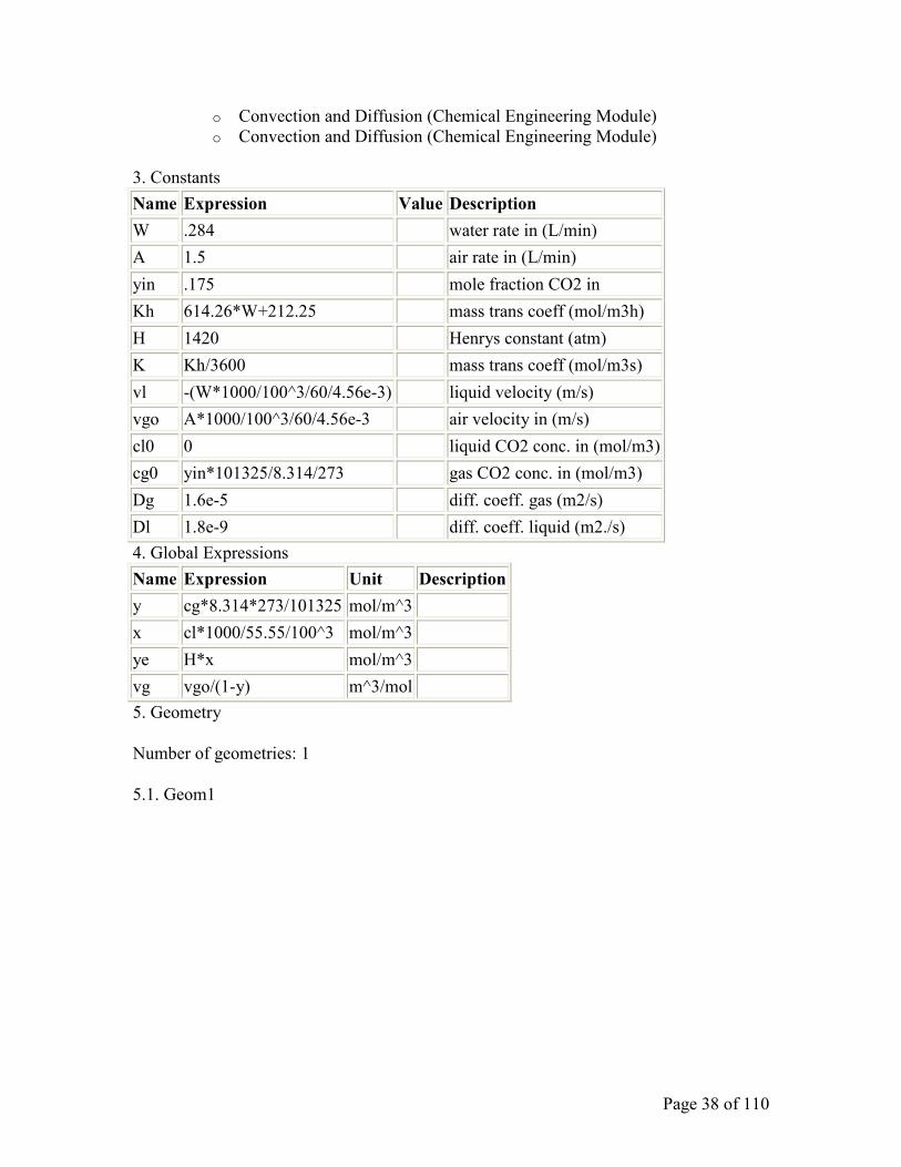
3. Constants
Name Expression Value Description
W .284 water rate in (L/min)
A 1.5 air rate in (L/min)
yin .175 mole fraction CO2 in
Kh 614.26*W+212.25 mass trans coeff (mol/m3h)
H 1420 Henrys constant (atm)
K Kh/3600 mass trans coeff (mol/m3s)
vl -(W*1000/100^3/60/4.56e-3) liquid velocity (m/s)
vgo A*1000/100^3/60/4.56e-3 air velocity in (m/s)
cl0 0 liquid CO2 conc. in (mol/m3)
cg0 yin*101325/8.314/273 gas CO2 conc. in (mol/m3)
Dg 1.6e-5 diff. coeff. gas (m2/s)
Dl 1.8e-9 diff. coeff. liquid (m2./s)
4. Global Expressions
Name Expression Unit Description
y cg*8.314*273/101325 mol/m^3
x cl*1000/55.55/100^3 mol/m^3
ye H*x mol/m^3
vg vgo/(1-y) m^3/mol
5. Geometry
Number of geometries: 1
5.1. Geom1

Page 39 of 110
5.1.1. Point mode

Page 40 of 110
5.1.2. Boundary mode

Page 41 of 110
5.1.3. Subdomain mode

Page 42 of 110
6. Geom1
Space dimensions: Axial symmetry (2D)
Independent variables: r, phi, z
6.1. Mesh
6.1.1. Mesh Statistics
Number of degrees of freedom 4098
Number of mesh points 545
Number of elements 960
Triangular 960
Quadrilateral 0
Number of boundary elements 128
Number of vertex elements 4
Minimum element quality 0.87
Element area ratio 0.75

Page 43 of 110
6.2. Application Mode: Convection and Diffusion (chcd)
Application mode type: Convection and Diffusion (Chemical Engineering Module)
Application mode name: chcd
6.2.1. Application Mode Properties
Property Value
Default element type Lagrange - Quadratic
Analysis type Stationary
Equation form Non-conservative
Equilibrium assumption Off
Frame Frame (ref)
Weak constraints Off
Constraint type Ideal
6.2.2. Variables
Dependent variables: cg
Page 44 of 110
Shape functions: shlag(2,'cg')
Interior boundaries not active
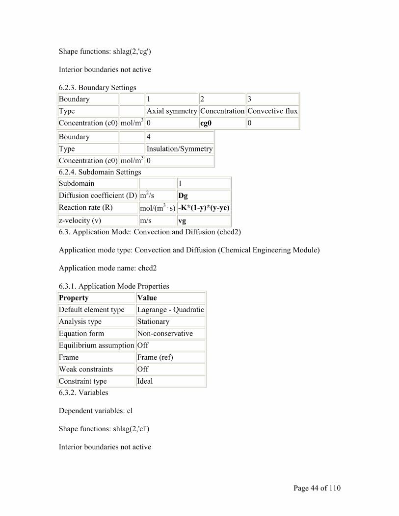
6.2.3. Boundary Settings
Boundary 1 2 3
Type Axial symmetry Concentration Convective flux
Concentration (c0) mol/m3 0 cg0 0
Boundary 4
Type Insulation/Symmetry
Concentration (c0) mol/m3 0
6.2.4. Subdomain Settings
Subdomain 1
Diffusion coefficient (D) m2/s Dg
Reaction rate (R) mol/(m3⋅s) -K*(1-y)*(y-ye)
z-velocity (v) m/s vg
6.3. Application Mode: Convection and Diffusion (chcd2)
Application mode type: Convection and Diffusion (Chemical Engineering Module)
Application mode name: chcd2
6.3.1. Application Mode Properties
Property Value
Default element type Lagrange - Quadratic
Analysis type Stationary
Equation form Non-conservative
Equilibrium assumption Off
Frame Frame (ref)
Weak constraints Off
Constraint type Ideal
6.3.2. Variables
Dependent variables: cl
Shape functions: shlag(2,'cl')
Interior boundaries not active
Page 45 of 110
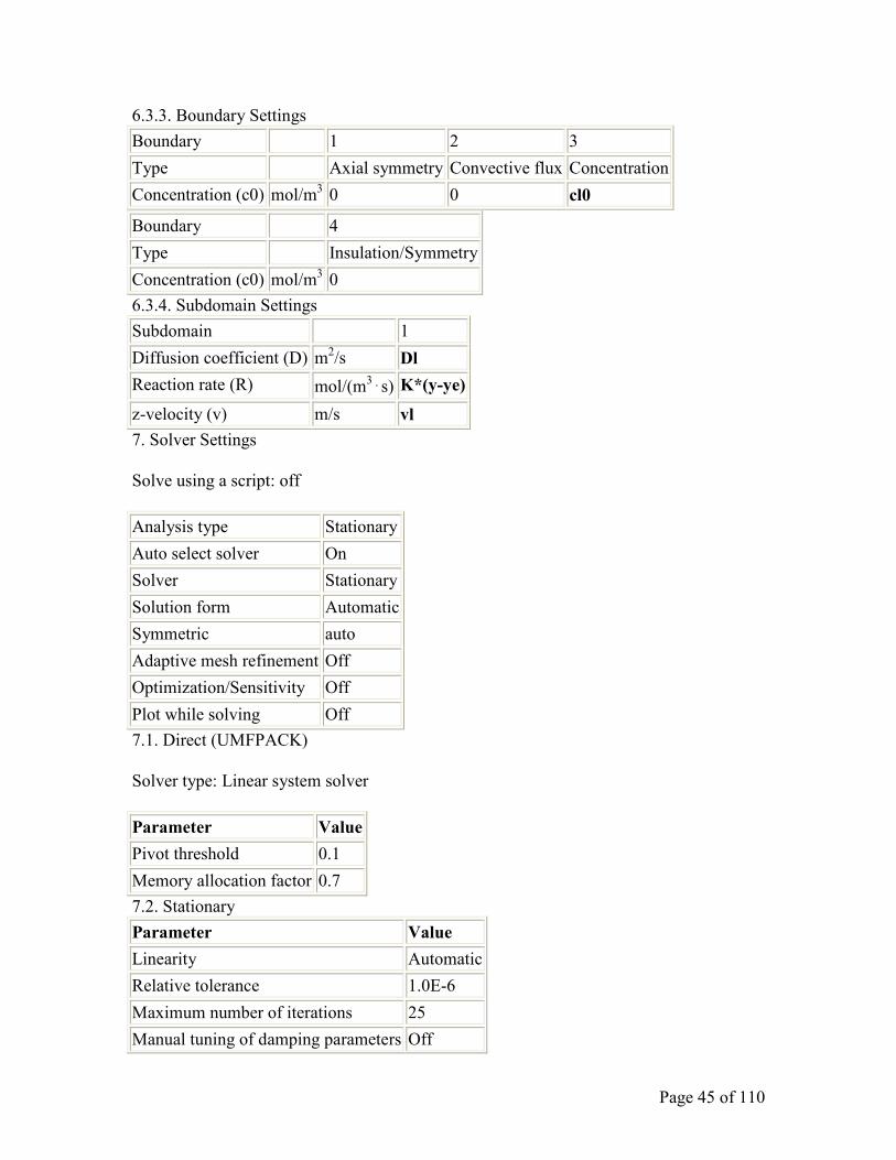
6.3.3. Boundary Settings
Boundary 1 2 3
Type Axial symmetry Convective flux Concentration
Concentration (c0) mol/m3 0 0 cl0
Boundary 4
Type Insulation/Symmetry
Concentration (c0) mol/m3 0
6.3.4. Subdomain Settings
Subdomain 1
Diffusion coefficient (D) m2/s Dl
Reaction rate (R) mol/(m3⋅s) K*(y-ye)
z-velocity (v) m/s vl
7. Solver Settings
Solve using a script: off
Analysis type Stationary
Auto select solver On
Solver Stationary
Solution form Automatic
Symmetric auto
Adaptive mesh refinement Off
Optimization/Sensitivity Off
Plot while solving Off
7.1. Direct (UMFPACK)
Solver type: Linear system solver
Parameter Value
Pivot threshold 0.1
Memory allocation factor 0.7
7.2. Stationary
Parameter Value
Linearity Automatic
Relative tolerance 1.0E-6
Maximum number of iterations 25
Manual tuning of damping parameters Off
Page 46 of 110
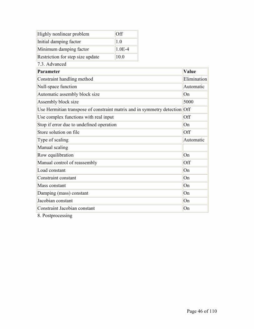
Highly nonlinear problem Off
Initial damping factor 1.0
Minimum damping factor 1.0E-4
Restriction for step size update 10.0
7.3. Advanced
Parameter Value
Constraint handling method Elimination
Null-space function Automatic
Automatic assembly block size On
Assembly block size 5000
Use Hermitian transpose of constraint matrix and in symmetry detection Off
Use complex functions with real input Off
Stop if error due to undefined operation On
Store solution on file Off
Type of scaling Automatic
Manual scaling
Row equilibration On
Manual control of reassembly Off
Load constant On
Constraint constant On
Mass constant On
Damping (mass) constant On
Jacobian constant On
Constraint Jacobian constant On
8. Postprocessing
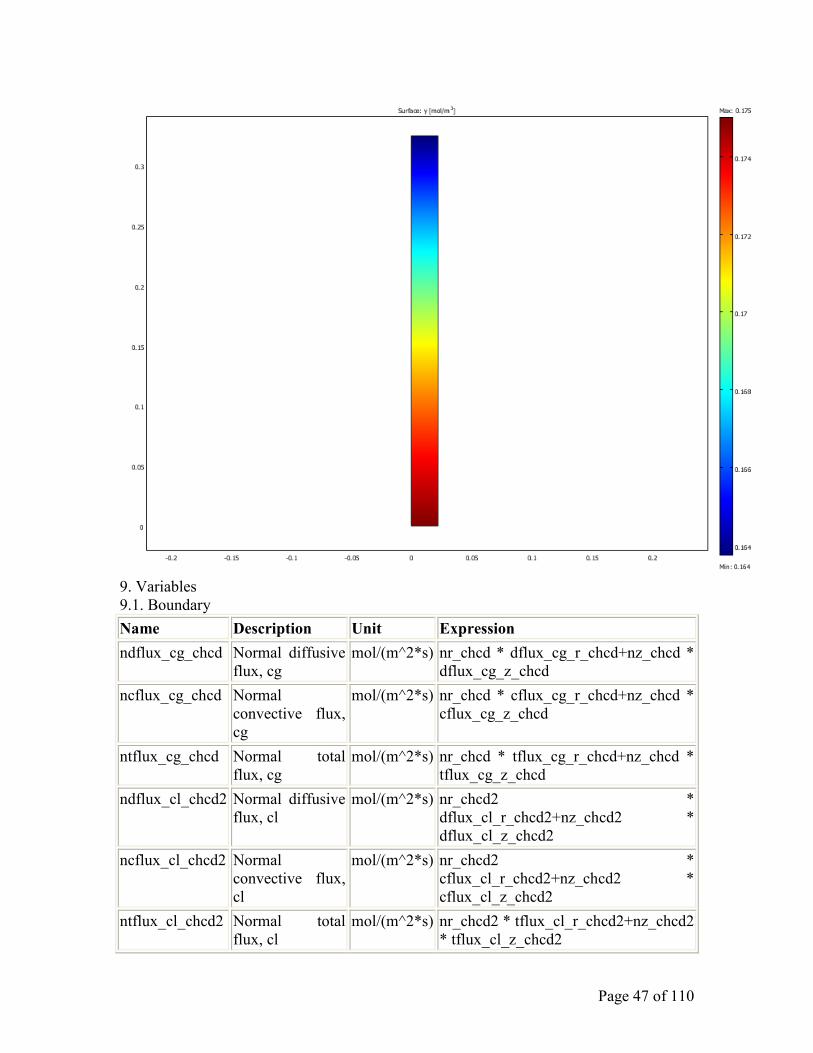
Page 47 of 110
9. Variables
9.1. Boundary
Name Description Unit Expression
ndflux_cg_chcd Normal diffusive
flux, cg
mol/(m^2*s) nr_chcd * dflux_cg_r_chcd+nz_chcd *
dflux_cg_z_chcd
ncflux_cg_chcd Normal
convective flux,
cg
mol/(m^2*s) nr_chcd * cflux_cg_r_chcd+nz_chcd *
cflux_cg_z_chcd
ntflux_cg_chcd Normal total
flux, cg
mol/(m^2*s) nr_chcd * tflux_cg_r_chcd+nz_chcd *
tflux_cg_z_chcd
ndflux_cl_chcd2 Normal diffusive
flux, cl
mol/(m^2*s) nr_chcd2 *
dflux_cl_r_chcd2+nz_chcd2 *
dflux_cl_z_chcd2
ncflux_cl_chcd2 Normal
convective flux,
cl
mol/(m^2*s) nr_chcd2 *
cflux_cl_r_chcd2+nz_chcd2 *
cflux_cl_z_chcd2
ntflux_cl_chcd2 Normal total
flux, cl
mol/(m^2*s) nr_chcd2 * tflux_cl_r_chcd2+nz_chcd2
* tflux_cl_z_chcd2
Page 48 of 110
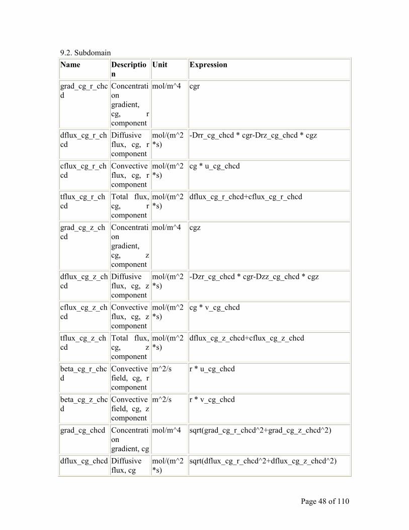
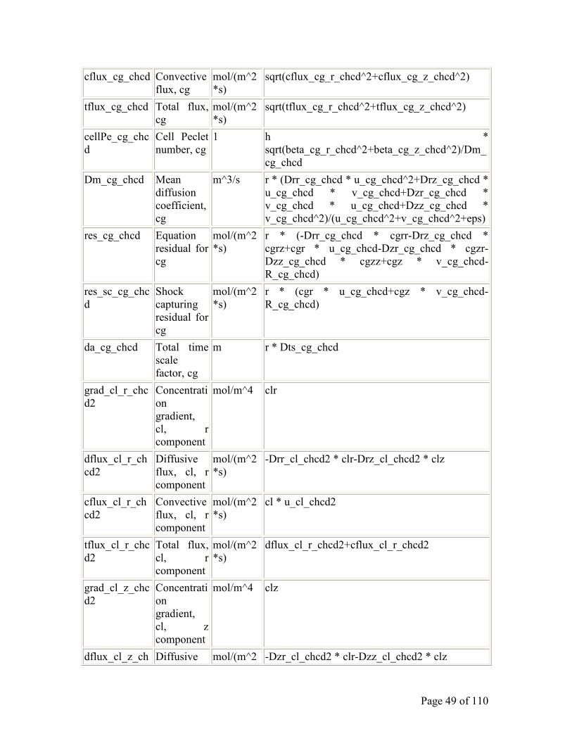
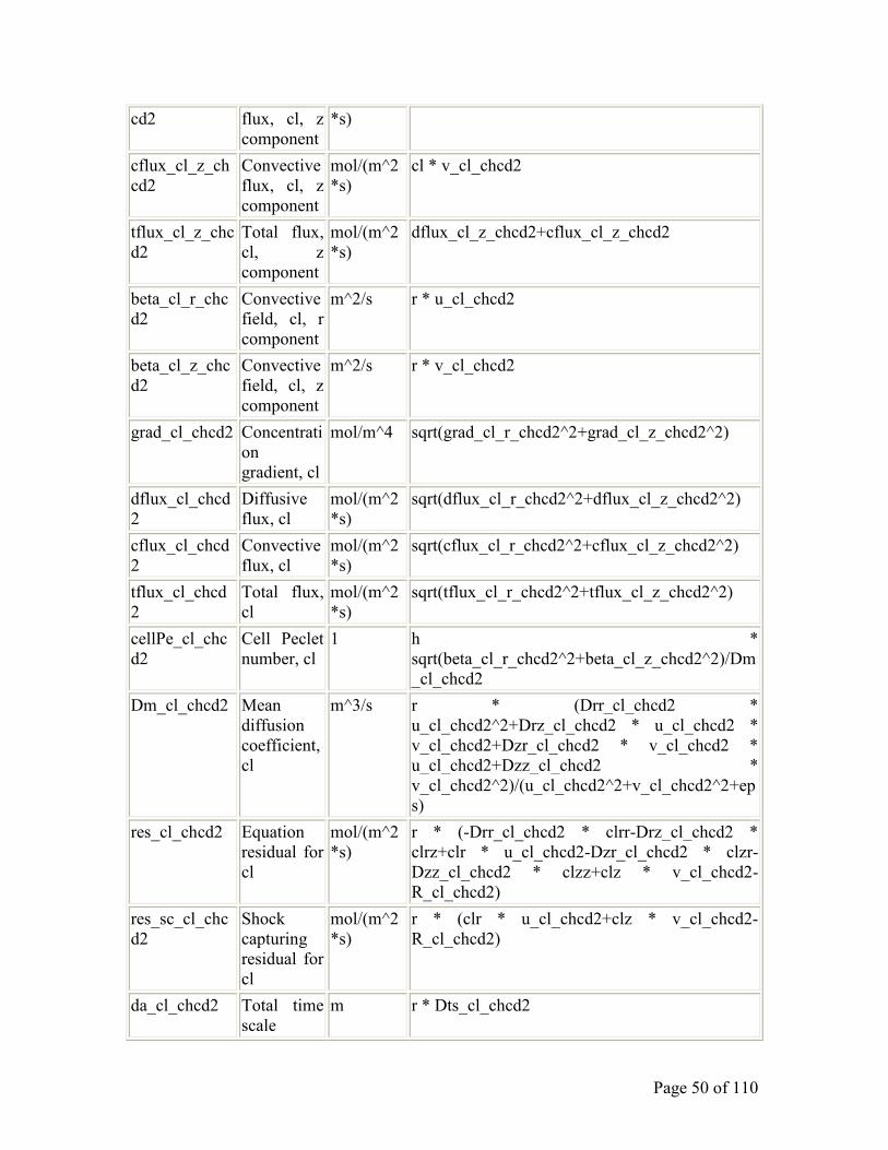
9.2. Subdomain
Name Descriptio
n
Unit Expression
grad_cg_r_chc
d
Concentrati
on
gradient,
cg, r
component
mol/m^4 cgr
dflux_cg_r_ch
cd
Diffusive
flux, cg, r
component
mol/(m^2
*s)
-Drr_cg_chcd * cgr-Drz_cg_chcd * cgz
cflux_cg_r_ch
cd
Convective
flux, cg, r
component
mol/(m^2
*s)
cg * u_cg_chcd
tflux_cg_r_ch
cd
Total flux,
cg, r
component
mol/(m^2
*s)
dflux_cg_r_chcd+cflux_cg_r_chcd
grad_cg_z_ch
cd
Concentrati
on
gradient,
cg, z
component
mol/m^4 cgz
dflux_cg_z_ch
cd
Diffusive
flux, cg, z
component
mol/(m^2
*s)
-Dzr_cg_chcd * cgr-Dzz_cg_chcd * cgz
cflux_cg_z_ch
cd
Convective
flux, cg, z
component
mol/(m^2
*s)
cg * v_cg_chcd
tflux_cg_z_ch
cd
Total flux,
cg, z
component
mol/(m^2
*s)
dflux_cg_z_chcd+cflux_cg_z_chcd
beta_cg_r_chc
d
Convective
field, cg, r
component
m^2/s r * u_cg_chcd
beta_cg_z_chc
d
Convective
field, cg, z
component
m^2/s r * v_cg_chcd
grad_cg_chcd Concentrati
on
gradient, cg
mol/m^4 sqrt(grad_cg_r_chcd^2+grad_cg_z_chcd^2)
dflux_cg_chcd Diffusive
flux, cg
mol/(m^2
*s)
sqrt(dflux_cg_r_chcd^2+dflux_cg_z_chcd^2)
Page 49 of 110
cflux_cg_chcd Convective
flux, cg
mol/(m^2
*s)
sqrt(cflux_cg_r_chcd^2+cflux_cg_z_chcd^2)
tflux_cg_chcd Total flux,
cg
mol/(m^2
*s)
sqrt(tflux_cg_r_chcd^2+tflux_cg_z_chcd^2)
cellPe_cg_chc
d
Cell Peclet
number, cg
1 h *
sqrt(beta_cg_r_chcd^2+beta_cg_z_chcd^2)/Dm_
cg_chcd
Dm_cg_chcd Mean
diffusion
coefficient,
cg
m^3/s r * (Drr_cg_chcd * u_cg_chcd^2+Drz_cg_chcd *
u_cg_chcd * v_cg_chcd+Dzr_cg_chcd *
v_cg_chcd * u_cg_chcd+Dzz_cg_chcd *
v_cg_chcd^2)/(u_cg_chcd^2+v_cg_chcd^2+eps)
res_cg_chcd Equation
residual for
cg
mol/(m^2
*s)
r * (-Drr_cg_chcd * cgrr-Drz_cg_chcd *
cgrz+cgr * u_cg_chcd-Dzr_cg_chcd * cgzr-
Dzz_cg_chcd * cgzz+cgz * v_cg_chcd-
R_cg_chcd)
res_sc_cg_chc
d
Shock
capturing
residual for
cg
mol/(m^2
*s)
r * (cgr * u_cg_chcd+cgz * v_cg_chcd-
R_cg_chcd)
da_cg_chcd Total time
scale
factor, cg
m r * Dts_cg_chcd
grad_cl_r_chc
d2
Concentrati
on
gradient,
cl, r
component
mol/m^4 clr
dflux_cl_r_ch
cd2
Diffusive
flux, cl, r
component
mol/(m^2
*s)
-Drr_cl_chcd2 * clr-Drz_cl_chcd2 * clz
cflux_cl_r_ch
cd2
Convective
flux, cl, r
component
mol/(m^2
*s)
cl * u_cl_chcd2
tflux_cl_r_chc
d2
Total flux,
cl, r
component
mol/(m^2
*s)
dflux_cl_r_chcd2+cflux_cl_r_chcd2
grad_cl_z_chc
d2
Concentrati
on
gradient,
cl, z
component
mol/m^4 clz
dflux_cl_z_ch Diffusive mol/(m^2 -Dzr_cl_chcd2 * clr-Dzz_cl_chcd2 * clz
Page 50 of 110
cd2 flux, cl, z
component
*s)
cflux_cl_z_ch
cd2
Convective
flux, cl, z
component
mol/(m^2
*s)
cl * v_cl_chcd2
tflux_cl_z_chc
d2
Total flux,
cl, z
component
mol/(m^2
*s)
dflux_cl_z_chcd2+cflux_cl_z_chcd2
beta_cl_r_chc
d2
Convective
field, cl, r
component
m^2/s r * u_cl_chcd2
beta_cl_z_chc
d2
Convective
field, cl, z
component
m^2/s r * v_cl_chcd2
grad_cl_chcd2 Concentrati
on
gradient, cl
mol/m^4 sqrt(grad_cl_r_chcd2^2+grad_cl_z_chcd2^2)
dflux_cl_chcd
2
Diffusive
flux, cl
mol/(m^2
*s)
sqrt(dflux_cl_r_chcd2^2+dflux_cl_z_chcd2^2)
cflux_cl_chcd
2
Convective
flux, cl
mol/(m^2
*s)
sqrt(cflux_cl_r_chcd2^2+cflux_cl_z_chcd2^2)
tflux_cl_chcd
2
Total flux,
cl
mol/(m^2
*s)
sqrt(tflux_cl_r_chcd2^2+tflux_cl_z_chcd2^2)
cellPe_cl_chc
d2
Cell Peclet
number, cl
1 h *
sqrt(beta_cl_r_chcd2^2+beta_cl_z_chcd2^2)/Dm
_cl_chcd2
Dm_cl_chcd2 Mean
diffusion
coefficient,
cl
m^3/s r * (Drr_cl_chcd2 *
u_cl_chcd2^2+Drz_cl_chcd2 * u_cl_chcd2 *
v_cl_chcd2+Dzr_cl_chcd2 * v_cl_chcd2 *
u_cl_chcd2+Dzz_cl_chcd2 *
v_cl_chcd2^2)/(u_cl_chcd2^2+v_cl_chcd2^2+ep
s)
res_cl_chcd2 Equation
residual for
cl
mol/(m^2
*s)
r * (-Drr_cl_chcd2 * clrr-Drz_cl_chcd2 *
clrz+clr * u_cl_chcd2-Dzr_cl_chcd2 * clzr-
Dzz_cl_chcd2 * clzz+clz * v_cl_chcd2-
R_cl_chcd2)
res_sc_cl_chc
d2
Shock
capturing
residual for
cl
mol/(m^2
*s)
r * (clr * u_cl_chcd2+clz * v_cl_chcd2-
R_cl_chcd2)
da_cl_chcd2 Total time
scale
m r * Dts_cl_chcd2

Page 51 of 110
factor, cl

Page 52 of 110
9 Appendix 3: Mini-Absorber, Lumped Parameter Model for Absorption/Reaction
COMSOL Model Report
1. Table of Contents
Title - COMSOL Model Report
Table of Contents
Model Properties
Constants
Global Expressions
Geometry
Geom1
Solver Settings
Postprocessing
Variables
2. Model Properties
Property Value
Model name
Author
Company
Department
Reference
URL
Saved date Apr 16, 2009 9:51:35 PM
Creation date Jun 11, 2008 1:16:28 PM
COMSOL version COMSOL 3.5.0.603
File name: R:\Absorption\absorber-mini-rxn.mph
Application modes and modules used in this model:
• Geom1 (Axial symmetry (2D))
Page 53 of 110
o Convection and Diffusion (Chemical Engineering Module)
o Convection and Diffusion (Chemical Engineering Module)
o Convection and Diffusion (Chemical Engineering Module)
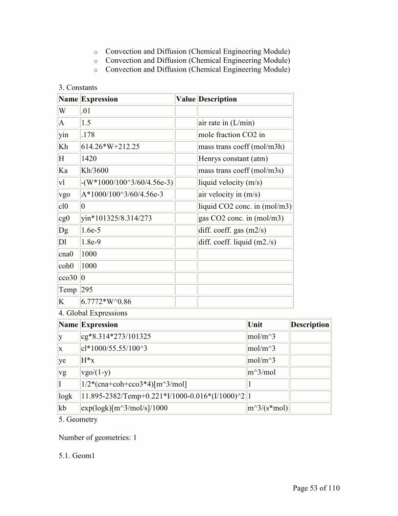
3. Constants
Name Expression Value Description
W .01
A 1.5 air rate in (L/min)
yin .178 mole fraction CO2 in
Kh 614.26*W+212.25 mass trans coeff (mol/m3h)
H 1420 Henrys constant (atm)
Ka Kh/3600 mass trans coeff (mol/m3s)
vl -(W*1000/100^3/60/4.56e-3) liquid velocity (m/s)
vgo A*1000/100^3/60/4.56e-3 air velocity in (m/s)
cl0 0 liquid CO2 conc. in (mol/m3)
cg0 yin*101325/8.314/273 gas CO2 conc. in (mol/m3)
Dg 1.6e-5 diff. coeff. gas (m2/s)
Dl 1.8e-9 diff. coeff. liquid (m2./s)
cna0 1000
coh0 1000
cco30 0
Temp 295
K 6.7772*W^0.86
4. Global Expressions
Name Expression Unit Description
y cg*8.314*273/101325 mol/m^3
x cl*1000/55.55/100^3 mol/m^3
ye H*x mol/m^3
vg vgo/(1-y) m^3/mol
I 1/2*(cna+coh+cco3*4)[m^3/mol] 1
logk 11.895-2382/Temp+0.221*I/1000-0.016*(I/1000)^2 1
kb exp(logk)[m^3/mol/s]/1000 m^3/(s*mol)
5. Geometry
Number of geometries: 1
5.1. Geom1
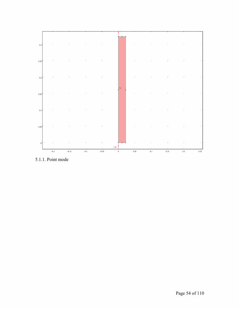
Page 54 of 110
5.1.1. Point mode

Page 55 of 110
5.1.2. Boundary mode

Page 56 of 110
5.1.3. Subdomain mode
Page 57 of 110
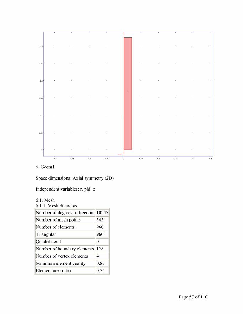
6. Geom1
Space dimensions: Axial symmetry (2D)
Independent variables: r, phi, z
6.1. Mesh
6.1.1. Mesh Statistics
Number of degrees of freedom 10245
Number of mesh points 545
Number of elements 960
Triangular 960
Quadrilateral 0
Number of boundary elements 128
Number of vertex elements 4
Minimum element quality 0.87
Element area ratio 0.75
Page 58 of 110
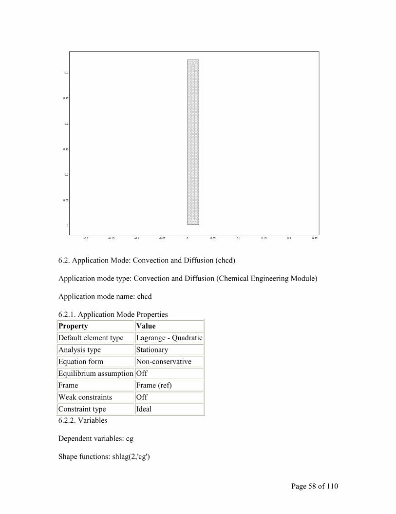
6.2. Application Mode: Convection and Diffusion (chcd)
Application mode type: Convection and Diffusion (Chemical Engineering Module)
Application mode name: chcd
6.2.1. Application Mode Properties
Property Value
Default element type Lagrange - Quadratic
Analysis type Stationary
Equation form Non-conservative
Equilibrium assumption Off
Frame Frame (ref)
Weak constraints Off
Constraint type Ideal
6.2.2. Variables
Dependent variables: cg
Shape functions: shlag(2,'cg')
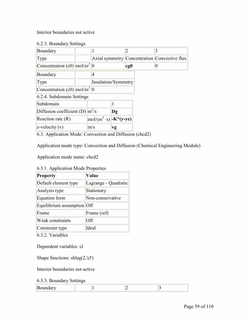
Page 59 of 110
Interior boundaries not active
6.2.3. Boundary Settings
Boundary 1 2 3
Type Axial symmetry Concentration Convective flux
Concentration (c0) mol/m3 0 cg0 0
Boundary 4
Type Insulation/Symmetry
Concentration (c0) mol/m3 0
6.2.4. Subdomain Settings
Subdomain 1
Diffusion coefficient (D) m2/s Dg
Reaction rate (R) mol/(m3⋅s) -K*(y-ye)
z-velocity (v) m/s vg
6.3. Application Mode: Convection and Diffusion (chcd2)
Application mode type: Convection and Diffusion (Chemical Engineering Module)
Application mode name: chcd2
6.3.1. Application Mode Properties
Property Value
Default element type Lagrange - Quadratic
Analysis type Stationary
Equation form Non-conservative
Equilibrium assumption Off
Frame Frame (ref)
Weak constraints Off
Constraint type Ideal
6.3.2. Variables
Dependent variables: cl
Shape functions: shlag(2,'cl')
Interior boundaries not active
6.3.3. Boundary Settings
Boundary 1 2 3
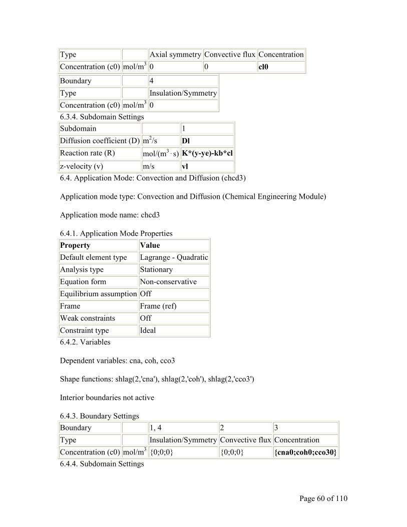
Page 60 of 110
Type Axial symmetry Convective flux Concentration
Concentration (c0) mol/m3 0 0 cl0
Boundary 4
Type Insulation/Symmetry
Concentration (c0) mol/m3 0
6.3.4. Subdomain Settings
Subdomain 1
Diffusion coefficient (D) m2/s Dl
Reaction rate (R) mol/(m3⋅s) K*(y-ye)-kb*cl
z-velocity (v) m/s vl
6.4. Application Mode: Convection and Diffusion (chcd3)
Application mode type: Convection and Diffusion (Chemical Engineering Module)
Application mode name: chcd3
6.4.1. Application Mode Properties
Property Value
Default element type Lagrange - Quadratic
Analysis type Stationary
Equation form Non-conservative
Equilibrium assumption Off
Frame Frame (ref)
Weak constraints Off
Constraint type Ideal
6.4.2. Variables
Dependent variables: cna, coh, cco3
Shape functions: shlag(2,'cna'), shlag(2,'coh'), shlag(2,'cco3')
Interior boundaries not active
6.4.3. Boundary Settings
Boundary 1, 4 2 3
Type Insulation/Symmetry Convective flux Concentration
Concentration (c0) mol/m3 {0;0;0} {0;0;0} {cna0;coh0;cco30}
6.4.4. Subdomain Settings
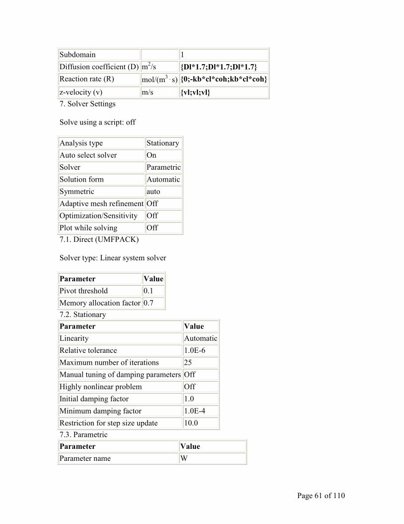
Page 61 of 110
Subdomain 1
Diffusion coefficient (D) m2/s {Dl*1.7;Dl*1.7;Dl*1.7}
Reaction rate (R) mol/(m3⋅s) {0;-kb*cl*coh;kb*cl*coh}
z-velocity (v) m/s {vl;vl;vl}
7. Solver Settings
Solve using a script: off
Analysis type Stationary
Auto select solver On
Solver Parametric
Solution form Automatic
Symmetric auto
Adaptive mesh refinement Off
Optimization/Sensitivity Off
Plot while solving Off
7.1. Direct (UMFPACK)
Solver type: Linear system solver
Parameter Value
Pivot threshold 0.1
Memory allocation factor 0.7
7.2. Stationary
Parameter Value
Linearity Automatic
Relative tolerance 1.0E-6
Maximum number of iterations 25
Manual tuning of damping parameters Off
Highly nonlinear problem Off
Initial damping factor 1.0
Minimum damping factor 1.0E-4
Restriction for step size update 10.0
7.3. Parametric
Parameter Value
Parameter name W

Page 62 of 110
Parameter values range(0.1,0.01,0.45)
Predictor Linear
Manual tuning of parameter step size Off
Initial step size 0.0
Minimum step size 0.0
Maximum step size 0.0
7.4. Advanced
Parameter Value
Constraint handling method Elimination
Null-space function Automatic
Automatic assembly block size On
Assembly block size 5000
Use Hermitian transpose of constraint matrix and in symmetry detection Off
Use complex functions with real input Off
Stop if error due to undefined operation On
Store solution on file Off
Type of scaling Automatic
Manual scaling
Row equilibration On
Manual control of reassembly Off
Load constant On
Constraint constant On
Mass constant On
Damping (mass) constant On
Jacobian constant On
Constraint Jacobian constant On
8. Postprocessing

Page 63 of 110
9. Variables
9.1. Boundary
Name Description Unit Expression
ndflux_cg_chcd Normal
diffusive flux,
cg
mol/(m^2*s) nr_chcd * dflux_cg_r_chcd+nz_chcd
* dflux_cg_z_chcd
ncflux_cg_chcd Normal
convective
flux, cg
mol/(m^2*s) nr_chcd * cflux_cg_r_chcd+nz_chcd
* cflux_cg_z_chcd
ntflux_cg_chcd Normal total
flux, cg
mol/(m^2*s) nr_chcd * tflux_cg_r_chcd+nz_chcd *
tflux_cg_z_chcd
ndflux_cl_chcd2 Normal
diffusive flux,
cl
mol/(m^2*s) nr_chcd2 *
dflux_cl_r_chcd2+nz_chcd2 *
dflux_cl_z_chcd2
ncflux_cl_chcd2 Normal
convective
flux, cl
mol/(m^2*s) nr_chcd2 *
cflux_cl_r_chcd2+nz_chcd2 *
cflux_cl_z_chcd2
ntflux_cl_chcd2 Normal total
flux, cl
mol/(m^2*s) nr_chcd2 *
tflux_cl_r_chcd2+nz_chcd2 *
tflux_cl_z_chcd2
ndflux_cna_chcd3 Normal mol/(m^2*s) nr_chcd3 *
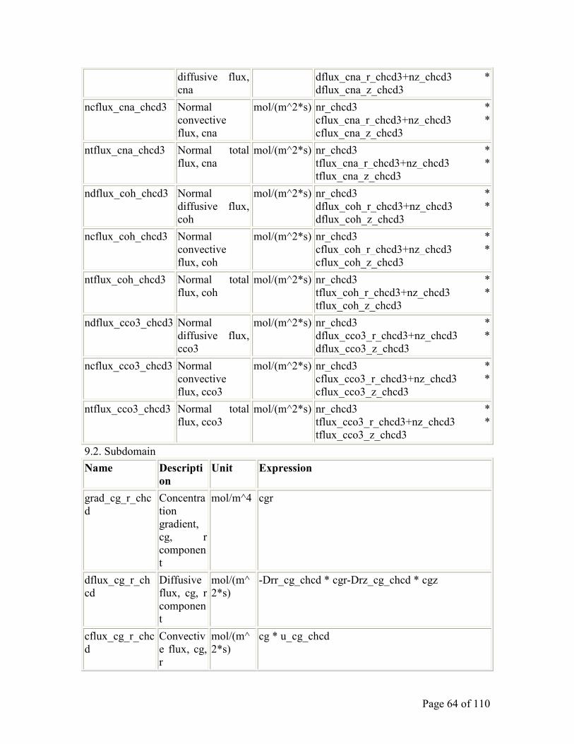
Page 64 of 110
diffusive flux,
cna
dflux_cna_r_chcd3+nz_chcd3 *
dflux_cna_z_chcd3
ncflux_cna_chcd3 Normal
convective
flux, cna
mol/(m^2*s) nr_chcd3 *
cflux_cna_r_chcd3+nz_chcd3 *
cflux_cna_z_chcd3
ntflux_cna_chcd3 Normal total
flux, cna
mol/(m^2*s) nr_chcd3 *
tflux_cna_r_chcd3+nz_chcd3 *
tflux_cna_z_chcd3
ndflux_coh_chcd3 Normal
diffusive flux,
coh
mol/(m^2*s) nr_chcd3 *
dflux_coh_r_chcd3+nz_chcd3 *
dflux_coh_z_chcd3
ncflux_coh_chcd3 Normal
convective
flux, coh
mol/(m^2*s) nr_chcd3 *
cflux_coh_r_chcd3+nz_chcd3 *
cflux_coh_z_chcd3
ntflux_coh_chcd3 Normal total
flux, coh
mol/(m^2*s) nr_chcd3 *
tflux_coh_r_chcd3+nz_chcd3 *
tflux_coh_z_chcd3
ndflux_cco3_chcd3 Normal
diffusive flux,
cco3
mol/(m^2*s) nr_chcd3 *
dflux_cco3_r_chcd3+nz_chcd3 *
dflux_cco3_z_chcd3
ncflux_cco3_chcd3 Normal
convective
flux, cco3
mol/(m^2*s) nr_chcd3 *
cflux_cco3_r_chcd3+nz_chcd3 *
cflux_cco3_z_chcd3
ntflux_cco3_chcd3 Normal total
flux, cco3
mol/(m^2*s) nr_chcd3 *
tflux_cco3_r_chcd3+nz_chcd3 *
tflux_cco3_z_chcd3
9.2. Subdomain
Name Descripti
on
Unit Expression
grad_cg_r_chc
d
Concentra
tion
gradient,
cg, r
componen
t
mol/m^4 cgr
dflux_cg_r_ch
cd
Diffusive
flux, cg, r
componen
t
mol/(m^
2*s)
-Drr_cg_chcd * cgr-Drz_cg_chcd * cgz
cflux_cg_r_chc
d
Convectiv
e flux, cg,
r
mol/(m^
2*s)
cg * u_cg_chcd
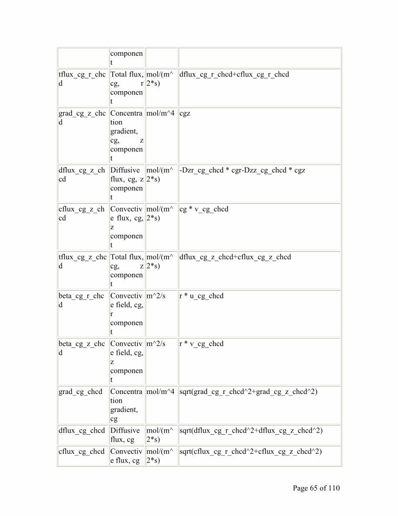
Page 65 of 110
componen
t
tflux_cg_r_chc
d
Total flux,
cg, r
componen
t
mol/(m^
2*s)
dflux_cg_r_chcd+cflux_cg_r_chcd
grad_cg_z_chc
d
Concentra
tion
gradient,
cg, z
componen
t
mol/m^4 cgz
dflux_cg_z_ch
cd
Diffusive
flux, cg, z
componen
t
mol/(m^
2*s)
-Dzr_cg_chcd * cgr-Dzz_cg_chcd * cgz
cflux_cg_z_ch
cd
Convectiv
e flux, cg,
z
componen
t
mol/(m^
2*s)
cg * v_cg_chcd
tflux_cg_z_chc
d
Total flux,
cg, z
componen
t
mol/(m^
2*s)
dflux_cg_z_chcd+cflux_cg_z_chcd
beta_cg_r_chc
d
Convectiv
e field, cg,
r
componen
t
m^2/s r * u_cg_chcd
beta_cg_z_chc
d
Convectiv
e field, cg,
z
componen
t
m^2/s r * v_cg_chcd
grad_cg_chcd Concentra
tion
gradient,
cg
mol/m^4 sqrt(grad_cg_r_chcd^2+grad_cg_z_chcd^2)
dflux_cg_chcd Diffusive
flux, cg
mol/(m^
2*s)
sqrt(dflux_cg_r_chcd^2+dflux_cg_z_chcd^2)
cflux_cg_chcd Convectiv
e flux, cg
mol/(m^
2*s)
sqrt(cflux_cg_r_chcd^2+cflux_cg_z_chcd^2)
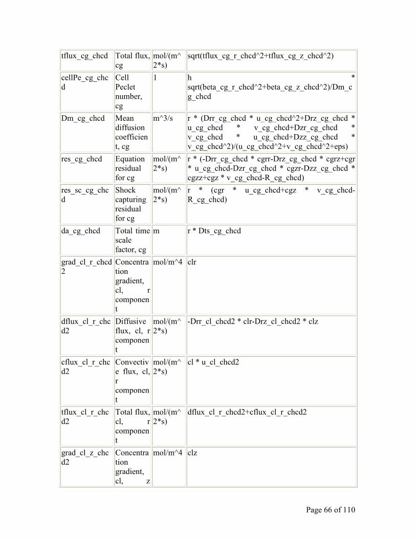
Page 66 of 110
tflux_cg_chcd Total flux,
cg
mol/(m^
2*s)
sqrt(tflux_cg_r_chcd^2+tflux_cg_z_chcd^2)
cellPe_cg_chc
d
Cell
Peclet
number,
cg
1 h *
sqrt(beta_cg_r_chcd^2+beta_cg_z_chcd^2)/Dm_c
g_chcd
Dm_cg_chcd Mean
diffusion
coefficien
t, cg
m^3/s r * (Drr_cg_chcd * u_cg_chcd^2+Drz_cg_chcd *
u_cg_chcd * v_cg_chcd+Dzr_cg_chcd *
v_cg_chcd * u_cg_chcd+Dzz_cg_chcd *
v_cg_chcd^2)/(u_cg_chcd^2+v_cg_chcd^2+eps)
res_cg_chcd Equation
residual
for cg
mol/(m^
2*s)
r * (-Drr_cg_chcd * cgrr-Drz_cg_chcd * cgrz+cgr
* u_cg_chcd-Dzr_cg_chcd * cgzr-Dzz_cg_chcd *
cgzz+cgz * v_cg_chcd-R_cg_chcd)
res_sc_cg_chc
d
Shock
capturing
residual
for cg
mol/(m^
2*s)
r * (cgr * u_cg_chcd+cgz * v_cg_chcd-
R_cg_chcd)
da_cg_chcd Total time
scale
factor, cg
m r * Dts_cg_chcd
grad_cl_r_chcd
2
Concentra
tion
gradient,
cl, r
componen
t
mol/m^4 clr
dflux_cl_r_chc
d2
Diffusive
flux, cl, r
componen
t
mol/(m^
2*s)
-Drr_cl_chcd2 * clr-Drz_cl_chcd2 * clz
cflux_cl_r_chc
d2
Convectiv
e flux, cl,
r
componen
t
mol/(m^
2*s)
cl * u_cl_chcd2
tflux_cl_r_chc
d2
Total flux,
cl, r
componen
t
mol/(m^
2*s)
dflux_cl_r_chcd2+cflux_cl_r_chcd2
grad_cl_z_chc
d2
Concentra
tion
gradient,
cl, z
mol/m^4 clz
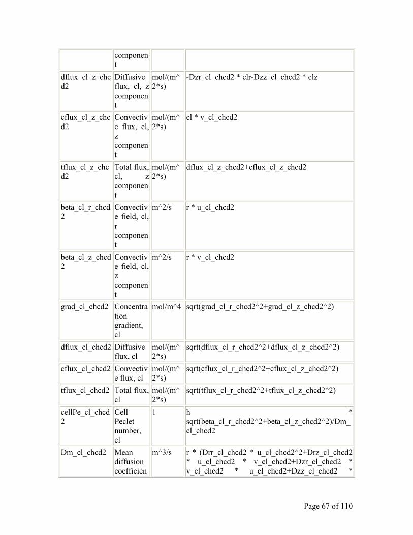
Page 67 of 110
componen
t
dflux_cl_z_chc
d2
Diffusive
flux, cl, z
componen
t
mol/(m^
2*s)
-Dzr_cl_chcd2 * clr-Dzz_cl_chcd2 * clz
cflux_cl_z_chc
d2
Convectiv
e flux, cl,
z
componen
t
mol/(m^
2*s)
cl * v_cl_chcd2
tflux_cl_z_chc
d2
Total flux,
cl, z
componen
t
mol/(m^
2*s)
dflux_cl_z_chcd2+cflux_cl_z_chcd2
beta_cl_r_chcd
2
Convectiv
e field, cl,
r
componen
t
m^2/s r * u_cl_chcd2
beta_cl_z_chcd
2
Convectiv
e field, cl,
z
componen
t
m^2/s r * v_cl_chcd2
grad_cl_chcd2 Concentra
tion
gradient,
cl
mol/m^4 sqrt(grad_cl_r_chcd2^2+grad_cl_z_chcd2^2)
dflux_cl_chcd2 Diffusive
flux, cl
mol/(m^
2*s)
sqrt(dflux_cl_r_chcd2^2+dflux_cl_z_chcd2^2)
cflux_cl_chcd2 Convectiv
e flux, cl
mol/(m^
2*s)
sqrt(cflux_cl_r_chcd2^2+cflux_cl_z_chcd2^2)
tflux_cl_chcd2 Total flux,
cl
mol/(m^
2*s)
sqrt(tflux_cl_r_chcd2^2+tflux_cl_z_chcd2^2)
cellPe_cl_chcd
2
Cell
Peclet
number,
cl
1 h *
sqrt(beta_cl_r_chcd2^2+beta_cl_z_chcd2^2)/Dm_
cl_chcd2
Dm_cl_chcd2 Mean
diffusion
coefficien
m^3/s r * (Drr_cl_chcd2 * u_cl_chcd2^2+Drz_cl_chcd2
* u_cl_chcd2 * v_cl_chcd2+Dzr_cl_chcd2 *
v_cl_chcd2 * u_cl_chcd2+Dzz_cl_chcd2 *

Page 68 of 110
t, cl v_cl_chcd2^2)/(u_cl_chcd2^2+v_cl_chcd2^2+eps)
res_cl_chcd2 Equation
residual
for cl
mol/(m^
2*s)
r * (-Drr_cl_chcd2 * clrr-Drz_cl_chcd2 * clrz+clr
* u_cl_chcd2-Dzr_cl_chcd2 * clzr-Dzz_cl_chcd2
* clzz+clz * v_cl_chcd2-R_cl_chcd2)
res_sc_cl_chcd
2
Shock
capturing
residual
for cl
mol/(m^
2*s)
r * (clr * u_cl_chcd2+clz * v_cl_chcd2-
R_cl_chcd2)
da_cl_chcd2 Total time
scale
factor, cl
m r * Dts_cl_chcd2
grad_cna_r_ch
cd3
Concentra
tion
gradient,
cna, r
componen
t
mol/m^4 cnar
dflux_cna_r_c
hcd3
Diffusive
flux, cna,
r
componen
t
mol/(m^
2*s)
-Drr_cna_chcd3 * cnar-Drz_cna_chcd3 * cnaz
cflux_cna_r_ch
cd3
Convectiv
e flux,
cna, r
componen
t
mol/(m^
2*s)
cna * u_cna_chcd3
tflux_cna_r_ch
cd3
Total flux,
cna, r
componen
t
mol/(m^
2*s)
dflux_cna_r_chcd3+cflux_cna_r_chcd3
grad_cna_z_ch
cd3
Concentra
tion
gradient,
cna, z
componen
t
mol/m^4 cnaz
dflux_cna_z_c
hcd3
Diffusive
flux, cna,
z
componen
t
mol/(m^
2*s)
-Dzr_cna_chcd3 * cnar-Dzz_cna_chcd3 * cnaz
cflux_cna_z_c Convectiv mol/(m^ cna * v_cna_chcd3
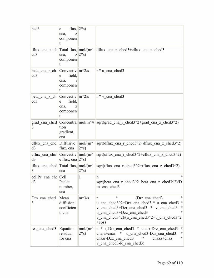
Page 69 of 110
hcd3 e flux,
cna, z
componen
t
2*s)
tflux_cna_z_ch
cd3
Total flux,
cna, z
componen
t
mol/(m^
2*s)
dflux_cna_z_chcd3+cflux_cna_z_chcd3
beta_cna_r_ch
cd3
Convectiv
e field,
cna, r
componen
t
m^2/s r * u_cna_chcd3
beta_cna_z_ch
cd3
Convectiv
e field,
cna, z
componen
t
m^2/s r * v_cna_chcd3
grad_cna_chcd
3
Concentra
tion
gradient,
cna
mol/m^4 sqrt(grad_cna_r_chcd3^2+grad_cna_z_chcd3^2)
dflux_cna_chc
d3
Diffusive
flux, cna
mol/(m^
2*s)
sqrt(dflux_cna_r_chcd3^2+dflux_cna_z_chcd3^2)
cflux_cna_chc
d3
Convectiv
e flux, cna
mol/(m^
2*s)
sqrt(cflux_cna_r_chcd3^2+cflux_cna_z_chcd3^2)
tflux_cna_chcd
3
Total flux,
cna
mol/(m^
2*s)
sqrt(tflux_cna_r_chcd3^2+tflux_cna_z_chcd3^2)
cellPe_cna_chc
d3
Cell
Peclet
number,
cna
1 h *
sqrt(beta_cna_r_chcd3^2+beta_cna_z_chcd3^2)/D
m_cna_chcd3
Dm_cna_chcd
3
Mean
diffusion
coefficien
t, cna
m^3/s r * (Drr_cna_chcd3 *
u_cna_chcd3^2+Drz_cna_chcd3 * u_cna_chcd3 *
v_cna_chcd3+Dzr_cna_chcd3 * v_cna_chcd3 *
u_cna_chcd3+Dzz_cna_chcd3 *
v_cna_chcd3^2)/(u_cna_chcd3^2+v_cna_chcd3^2
+eps)
res_cna_chcd3 Equation
residual
for cna
mol/(m^
2*s)
r * (-Drr_cna_chcd3 * cnarr-Drz_cna_chcd3 *
cnarz+cnar * u_cna_chcd3-Dzr_cna_chcd3 *
cnazr-Dzz_cna_chcd3 * cnazz+cnaz *
v_cna_chcd3-R_cna_chcd3)

Page 70 of 110
res_sc_cna_ch
cd3
Shock
capturing
residual
for cna
mol/(m^
2*s)
r * (cnar * u_cna_chcd3+cnaz * v_cna_chcd3-
R_cna_chcd3)
da_cna_chcd3 Total time
scale
factor, cna
m r * Dts_cna_chcd3
grad_coh_r_ch
cd3
Concentra
tion
gradient,
coh, r
componen
t
mol/m^4 cohr
dflux_coh_r_c
hcd3
Diffusive
flux, coh,
r
componen
t
mol/(m^
2*s)
-Drr_coh_chcd3 * cohr-Drz_coh_chcd3 * cohz
cflux_coh_r_c
hcd3
Convectiv
e flux,
coh, r
componen
t
mol/(m^
2*s)
coh * u_coh_chcd3
tflux_coh_r_ch
cd3
Total flux,
coh, r
componen
t
mol/(m^
2*s)
dflux_coh_r_chcd3+cflux_coh_r_chcd3
grad_coh_z_ch
cd3
Concentra
tion
gradient,
coh, z
componen
t
mol/m^4 cohz
dflux_coh_z_c
hcd3
Diffusive
flux, coh,
z
componen
t
mol/(m^
2*s)
-Dzr_coh_chcd3 * cohr-Dzz_coh_chcd3 * cohz
cflux_coh_z_c
hcd3
Convectiv
e flux,
coh, z
componen
t
mol/(m^
2*s)
coh * v_coh_chcd3

Page 71 of 110
tflux_coh_z_ch
cd3
Total flux,
coh, z
componen
t
mol/(m^
2*s)
dflux_coh_z_chcd3+cflux_coh_z_chcd3
beta_coh_r_ch
cd3
Convectiv
e field,
coh, r
componen
t
m^2/s r * u_coh_chcd3
beta_coh_z_ch
cd3
Convectiv
e field,
coh, z
componen
t
m^2/s r * v_coh_chcd3
grad_coh_chcd
3
Concentra
tion
gradient,
coh
mol/m^4 sqrt(grad_coh_r_chcd3^2+grad_coh_z_chcd3^2)
dflux_coh_chc
d3
Diffusive
flux, coh
mol/(m^
2*s)
sqrt(dflux_coh_r_chcd3^2+dflux_coh_z_chcd3^2)
cflux_coh_chc
d3
Convectiv
e flux, coh
mol/(m^
2*s)
sqrt(cflux_coh_r_chcd3^2+cflux_coh_z_chcd3^2)
tflux_coh_chcd
3
Total flux,
coh
mol/(m^
2*s)
sqrt(tflux_coh_r_chcd3^2+tflux_coh_z_chcd3^2)
cellPe_coh_ch
cd3
Cell
Peclet
number,
coh
1 h *
sqrt(beta_coh_r_chcd3^2+beta_coh_z_chcd3^2)/D
m_coh_chcd3
Dm_coh_chcd
3
Mean
diffusion
coefficien
t, coh
m^3/s r * (Drr_coh_chcd3 *
u_coh_chcd3^2+Drz_coh_chcd3 * u_coh_chcd3 *
v_coh_chcd3+Dzr_coh_chcd3 * v_coh_chcd3 *
u_coh_chcd3+Dzz_coh_chcd3 *
v_coh_chcd3^2)/(u_coh_chcd3^2+v_coh_chcd3^2
+eps)
res_coh_chcd3 Equation
residual
for coh
mol/(m^
2*s)
r * (-Drr_coh_chcd3 * cohrr-Drz_coh_chcd3 *
cohrz+cohr * u_coh_chcd3-Dzr_coh_chcd3 *
cohzr-Dzz_coh_chcd3 * cohzz+cohz *
v_coh_chcd3-R_coh_chcd3)
res_sc_coh_ch
cd3
Shock
capturing
residual
for coh
mol/(m^
2*s)
r * (cohr * u_coh_chcd3+cohz * v_coh_chcd3-
R_coh_chcd3)

Page 72 of 110
da_coh_chcd3 Total time
scale
factor,
coh
m r * Dts_coh_chcd3
grad_cco3_r_c
hcd3
Concentra
tion
gradient,
cco3, r
componen
t
mol/m^4 cco3r
dflux_cco3_r_
chcd3
Diffusive
flux, cco3,
r
componen
t
mol/(m^
2*s)
-Drr_cco3_chcd3 * cco3r-Drz_cco3_chcd3 *
cco3z
cflux_cco3_r_c
hcd3
Convectiv
e flux,
cco3, r
componen
t
mol/(m^
2*s)
cco3 * u_cco3_chcd3
tflux_cco3_r_c
hcd3
Total flux,
cco3, r
componen
t
mol/(m^
2*s)
dflux_cco3_r_chcd3+cflux_cco3_r_chcd3
grad_cco3_z_c
hcd3
Concentra
tion
gradient,
cco3, z
componen
t
mol/m^4 cco3z
dflux_cco3_z_
chcd3
Diffusive
flux, cco3,
z
componen
t
mol/(m^
2*s)
-Dzr_cco3_chcd3 * cco3r-Dzz_cco3_chcd3 *
cco3z
cflux_cco3_z_
chcd3
Convectiv
e flux,
cco3, z
componen
t
mol/(m^
2*s)
cco3 * v_cco3_chcd3
tflux_cco3_z_c
hcd3
Total flux,
cco3, z
componen
mol/(m^
2*s)
dflux_cco3_z_chcd3+cflux_cco3_z_chcd3

Page 73 of 110
t
beta_cco3_r_c
hcd3
Convectiv
e field,
cco3, r
componen
t
m^2/s r * u_cco3_chcd3
beta_cco3_z_c
hcd3
Convectiv
e field,
cco3, z
componen
t
m^2/s r * v_cco3_chcd3
grad_cco3_chc
d3
Concentra
tion
gradient,
cco3
mol/m^4 sqrt(grad_cco3_r_chcd3^2+grad_cco3_z_chcd3^2
)
dflux_cco3_ch
cd3
Diffusive
flux, cco3
mol/(m^
2*s)
sqrt(dflux_cco3_r_chcd3^2+dflux_cco3_z_chcd3^
2)
cflux_cco3_ch
cd3
Convectiv
e flux,
cco3
mol/(m^
2*s)
sqrt(cflux_cco3_r_chcd3^2+cflux_cco3_z_chcd3^
2)
tflux_cco3_chc
d3
Total flux,
cco3
mol/(m^
2*s)
sqrt(tflux_cco3_r_chcd3^2+tflux_cco3_z_chcd3^2
)
cellPe_cco3_c
hcd3
Cell
Peclet
number,
cco3
1 h *
sqrt(beta_cco3_r_chcd3^2+beta_cco3_z_chcd3^2)
/Dm_cco3_chcd3
Dm_cco3_chc
d3
Mean
diffusion
coefficien
t, cco3
m^3/s r * (Drr_cco3_chcd3 *
u_cco3_chcd3^2+Drz_cco3_chcd3 *
u_cco3_chcd3 * v_cco3_chcd3+Dzr_cco3_chcd3
* v_cco3_chcd3 *
u_cco3_chcd3+Dzz_cco3_chcd3 *
v_cco3_chcd3^2)/(u_cco3_chcd3^2+v_cco3_chcd
3^2+eps)
res_cco3_chcd
3
Equation
residual
for cco3
mol/(m^
2*s)
r * (-Drr_cco3_chcd3 * cco3rr-Drz_cco3_chcd3 *
cco3rz+cco3r * u_cco3_chcd3-Dzr_cco3_chcd3 *
cco3zr-Dzz_cco3_chcd3 * cco3zz+cco3z *
v_cco3_chcd3-R_cco3_chcd3)
res_sc_cco3_c
hcd3
Shock
capturing
residual
for cco3
mol/(m^
2*s)
r * (cco3r * u_cco3_chcd3+cco3z *
v_cco3_chcd3-R_cco3_chcd3)
da_cco3_chcd3 Total time m r * Dts_cco3_chcd3

Page 74 of 110
scale
factor,
cco3
Page 75 of 110
10 Appendix 4: Mini-Absorber, Two-Film Model for Absorption with Reaction
COMSOL Model Report
1. Table of Contents
• Title - COMSOL Model Report
• Table of Contents
• Model Properties
• Constants
• Global Expressions
• Geometry
• Geom1
• Solver Settings
• Postprocessing
• Variables
2. Model Properties
Property Value
Model name
Author
Company
Department
Reference
URL
Saved date Apr 23, 2009 2:32:58 PM
Creation date Apr 18, 2008 1:31:23 PM
COMSOL version COMSOL 3.5.0.603
File name: R:\Absorption\absorber-micro-mini-rxn.mph
Application modes and modules used in this model:
• Geom1 (Axial symmetry (2D))
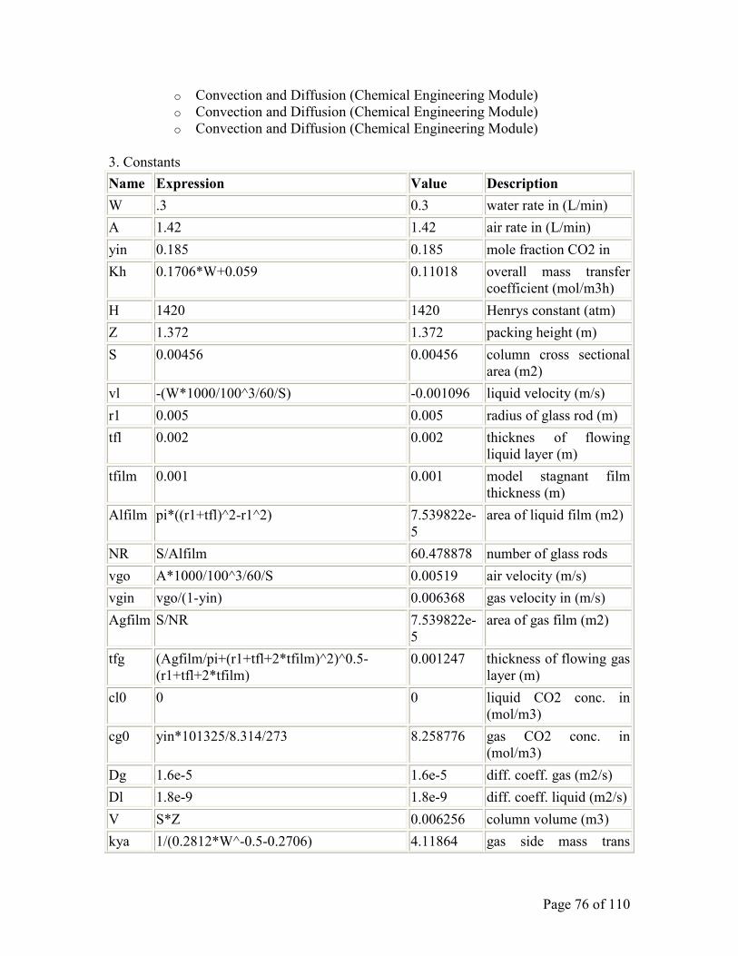
Page 76 of 110
o Convection and Diffusion (Chemical Engineering Module)
o Convection and Diffusion (Chemical Engineering Module)
o Convection and Diffusion (Chemical Engineering Module)
3. Constants
Name Expression Value Description
W .3 0.3 water rate in (L/min)
A 1.42 1.42 air rate in (L/min)
yin 0.185 0.185 mole fraction CO2 in
Kh 0.1706*W+0.059 0.11018 overall mass transfer
coefficient (mol/m3h)
H 1420 1420 Henrys constant (atm)
Z 1.372 1.372 packing height (m)
S 0.00456 0.00456 column cross sectional
area (m2)
vl -(W*1000/100^3/60/S) -0.001096 liquid velocity (m/s)
r1 0.005 0.005 radius of glass rod (m)
tfl 0.002 0.002 thicknes of flowing
liquid layer (m)
tfilm 0.001 0.001 model stagnant film
thickness (m)
Alfilm pi*((r1+tfl)^2-r1^2) 7.539822e-
5
area of liquid film (m2)
NR S/Alfilm 60.478878 number of glass rods
vgo A*1000/100^3/60/S 0.00519 air velocity (m/s)
vgin vgo/(1-yin) 0.006368 gas velocity in (m/s)
Agfilm S/NR 7.539822e-
5
area of gas film (m2)
tfg (Agfilm/pi+(r1+tfl+2*tfilm)^2)^0.5-
(r1+tfl+2*tfilm)
0.001247 thickness of flowing gas
layer (m)
cl0 0 0 liquid CO2 conc. in
(mol/m3)
cg0 yin*101325/8.314/273 8.258776 gas CO2 conc. in
(mol/m3)
Dg 1.6e-5 1.6e-5 diff. coeff. gas (m2/s)
Dl 1.8e-9 1.8e-9 diff. coeff. liquid (m2/s)
V S*Z 0.006256 column volume (m3)
kya 1/(0.2812*W^-0.5-0.2706) 4.11864 gas side mass trans

Page 77 of 110
coeff (mol/m3s)
Kya Kh/3600 3.060556e-
5
overall mass trans coeff
(mol/m3s)
kxa 1000000 10e5 liquid side mass trans
coeff (mol/m3s)
ia Z*2*pi*(r1+tfl+tfilm)*NR 4.17088 total interfacial area
(m2)
a ia/V 666.666667 interfacial area per
volume (m2/m3)
Deffg kya/a*tfilm/(101325/(8.314*273)) 1.383889e-
7
Effective diffusivity in
gas film (m2/s)
Deffl kxa/a*tfilm/(55.556*100^3/1000) 2.699978e-
5
Effective diffusivity in
liquid film (m2/s)
yout 0.099 0.099 mole fraction CO2 out
vgout vgo/(1-yout) 0.00576 gas velocity out (m/s)
vgave (vgin+vgout)/2 0.006064 average gas velocity
(m/s)
M 10000 10000 Stiff spring constant
tl Dl*tfilm/Deffl 6.66672e-8 predicted stagnant liquid
film thickness (m)
Cna0 1000 1000 liquid Na+ conc. in
(mol/m3)
Cco30 0 0 liquid CO3-2 conc in.
(mol/m3)
Coh0 2*Cna0 2000 liquid OH- conc. in
(mol/m3)
Temp 298 298
4. Global Expressions
Name Expression Unit Description
y cg*8.314*273/101325 mol/m^3
x cl*1000/55.55/100^3 mol/m^3
vg vgo/(1-y) m^3/mol
ye H*x mol/m^3
5. Geometry
Number of geometries: 1
5.1. Geom1
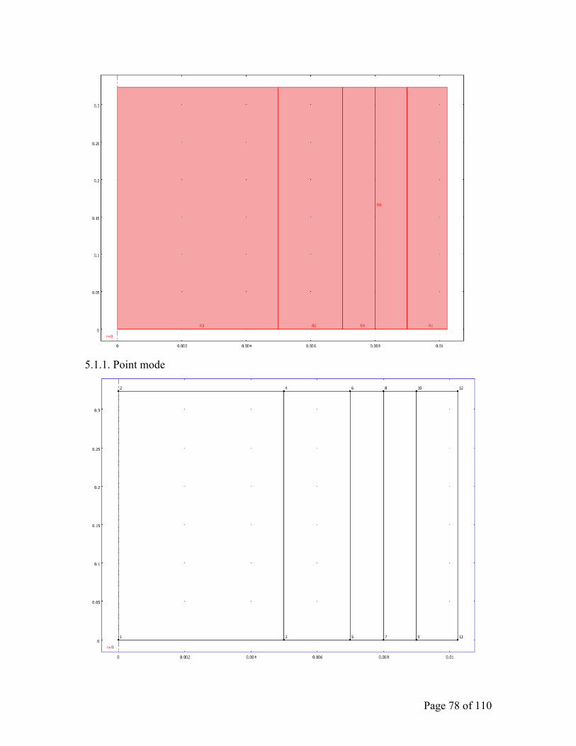
Page 78 of 110
5.1.1. Point mode

Page 79 of 110
5.1.2. Boundary mode
5.1.3. Subdomain mode
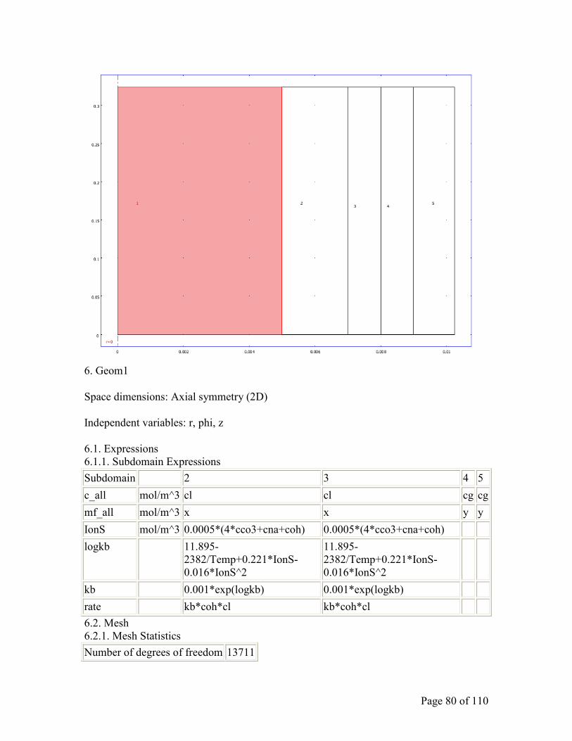
Page 80 of 110
6. Geom1
Space dimensions: Axial symmetry (2D)
Independent variables: r, phi, z
6.1. Expressions
6.1.1. Subdomain Expressions
Subdomain 2 3 4 5
c_all mol/m^3 cl cl cg cg
mf_all mol/m^3 x x y y
IonS mol/m^3 0.0005*(4*cco3+cna+coh) 0.0005*(4*cco3+cna+coh)
logkb 11.895-
2382/Temp+0.221*IonS-
0.016*IonS^2
11.895-
2382/Temp+0.221*IonS-
0.016*IonS^2
kb 0.001*exp(logkb) 0.001*exp(logkb)
rate kb*coh*cl kb*coh*cl
6.2. Mesh
6.2.1. Mesh Statistics
Number of degrees of freedom 13711

Page 81 of 110
Number of mesh points 1427
Number of elements 2600
Triangular 2600
Quadrilateral 0
Number of boundary elements 1067
Number of vertex elements 12
Minimum element quality 0.644
Element area ratio 0.018
6.3. Application Mode: Convection and Diffusion (chcd)
Application mode type: Convection and Diffusion (Chemical Engineering Module)
Application mode name: chcd
6.3.1. Application Mode Properties
Property Value
Default element type Lagrange - Quadratic
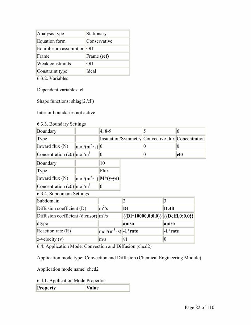
Page 82 of 110
Analysis type Stationary
Equation form Conservative
Equilibrium assumption Off
Frame Frame (ref)
Weak constraints Off
Constraint type Ideal
6.3.2. Variables
Dependent variables: cl
Shape functions: shlag(2,'cl')
Interior boundaries not active
6.3.3. Boundary Settings
Boundary 4, 8-9 5 6
Type Insulation/Symmetry Convective flux Concentration
Inward flux (N) mol/(m2⋅s) 0 0 0
Concentration (c0) mol/m3 0 0 cl0
Boundary 10
Type Flux
Inward flux (N) mol/(m2⋅s) M*(y-ye)
Concentration (c0) mol/m3 0
6.3.4. Subdomain Settings
Subdomain 2 3
Diffusion coefficient (D) m2/s Dl Deffl
Diffusion coefficient (dtensor) m2/s {{Dl*10000,0;0,0}} {{Deffl,0;0,0}}
dtype aniso aniso
Reaction rate (R) mol/(m3⋅s) -1*rate -1*rate
z-velocity (v) m/s vl 0
6.4. Application Mode: Convection and Diffusion (chcd2)
Application mode type: Convection and Diffusion (Chemical Engineering Module)
Application mode name: chcd2
6.4.1. Application Mode Properties
Property Value
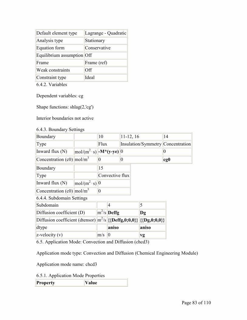
Page 83 of 110
Default element type Lagrange - Quadratic
Analysis type Stationary
Equation form Conservative
Equilibrium assumption Off
Frame Frame (ref)
Weak constraints Off
Constraint type Ideal
6.4.2. Variables
Dependent variables: cg
Shape functions: shlag(2,'cg')
Interior boundaries not active
6.4.3. Boundary Settings
Boundary 10 11-12, 16 14
Type Flux Insulation/Symmetry Concentration
Inward flux (N) mol/(m2⋅s) -M*(y-ye) 0 0
Concentration (c0) mol/m3 0 0 cg0
Boundary 15
Type Convective flux
Inward flux (N) mol/(m2⋅s) 0
Concentration (c0) mol/m3 0
6.4.4. Subdomain Settings
Subdomain 4 5
Diffusion coefficient (D) m2/s Deffg Dg
Diffusion coefficient (dtensor) m2/s {{Deffg,0;0,0}} {{Dg,0;0,0}}
dtype aniso aniso
z-velocity (v) m/s 0 vg
6.5. Application Mode: Convection and Diffusion (chcd3)
Application mode type: Convection and Diffusion (Chemical Engineering Module)
Application mode name: chcd3
6.5.1. Application Mode Properties
Property Value

Page 84 of 110
Default element type Lagrange - Quadratic
Analysis type Stationary
Equation form Conservative
Equilibrium assumption Off
Frame Frame (ref)
Weak constraints Off
Constraint type Ideal
6.5.2. Variables
Dependent variables: cco3, cna, coh
Shape functions: shlag(2,'cco3'), shlag(2,'cna'), shlag(2,'coh')
Interior boundaries not active
6.5.3. Boundary Settings
Boundary 4, 8-10 5 6
Type Insulation/Symmetry Convective flux Concentration
Concentration (c0) mol/m3 {0;0;0} {0;0;0} {Cco30;Cna0;Coh0}
6.5.4. Subdomain Settings
Subdom
ain
2 3
Diffusio
n
coefficie
nt
(dtensor)
m2/s {{1,0;0,1};{Dl*10000,0;0,1};{Dl*10000
*2,0;0,1}}
{{Deffl,0;0,1};{1,0;0,1};{1,
0;0,1}}
dtype {aniso;aniso;aniso} {aniso;aniso;aniso}
Reaction
rate (R)
mol/(m3
⋅s) {rate;0;-2*rate} {rate;0;-2*rate}
z-
velocity
(v)
m/s {vl;vl;vl} {0;0;0}
7. Solver Settings
Solve using a script: off
Analysis type Stationary
Auto select solver On
Solver Stationary
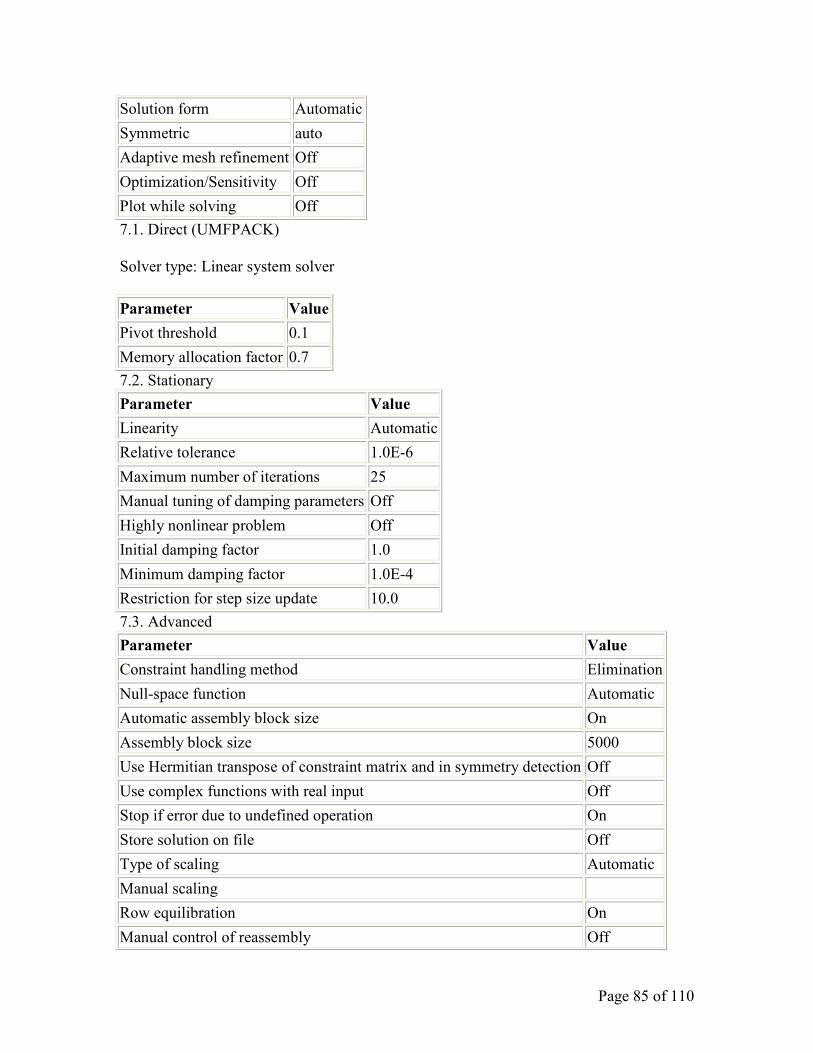
Page 85 of 110
Solution form Automatic
Symmetric auto
Adaptive mesh refinement Off
Optimization/Sensitivity Off
Plot while solving Off
7.1. Direct (UMFPACK)
Solver type: Linear system solver
Parameter Value
Pivot threshold 0.1
Memory allocation factor 0.7
7.2. Stationary
Parameter Value
Linearity Automatic
Relative tolerance 1.0E-6
Maximum number of iterations 25
Manual tuning of damping parameters Off
Highly nonlinear problem Off
Initial damping factor 1.0
Minimum damping factor 1.0E-4
Restriction for step size update 10.0
7.3. Advanced
Parameter Value
Constraint handling method Elimination
Null-space function Automatic
Automatic assembly block size On
Assembly block size 5000
Use Hermitian transpose of constraint matrix and in symmetry detection Off
Use complex functions with real input Off
Stop if error due to undefined operation On
Store solution on file Off
Type of scaling Automatic
Manual scaling
Row equilibration On
Manual control of reassembly Off
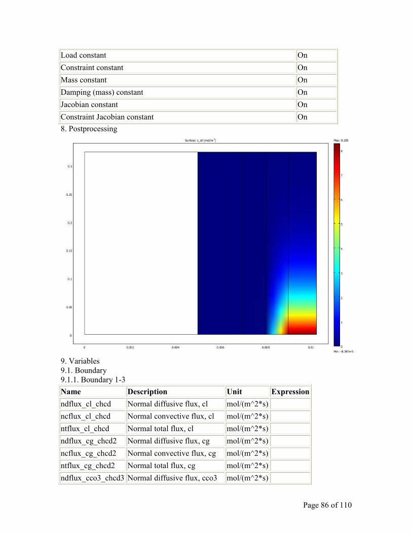
Page 86 of 110
Load constant On
Constraint constant On
Mass constant On
Damping (mass) constant On
Jacobian constant On
Constraint Jacobian constant On
8. Postprocessing
9. Variables
9.1. Boundary
9.1.1. Boundary 1-3
Name Description Unit Expression
ndflux_cl_chcd Normal diffusive flux, cl mol/(m^2*s)
ncflux_cl_chcd Normal convective flux, cl mol/(m^2*s)
ntflux_cl_chcd Normal total flux, cl mol/(m^2*s)
ndflux_cg_chcd2 Normal diffusive flux, cg mol/(m^2*s)
ncflux_cg_chcd2 Normal convective flux, cg mol/(m^2*s)
ntflux_cg_chcd2 Normal total flux, cg mol/(m^2*s)
ndflux_cco3_chcd3 Normal diffusive flux, cco3 mol/(m^2*s)
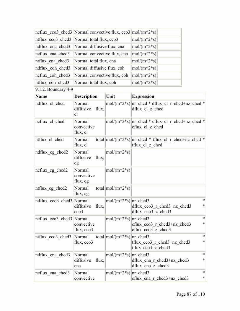
Page 87 of 110
ncflux_cco3_chcd3 Normal convective flux, cco3 mol/(m^2*s)
ntflux_cco3_chcd3 Normal total flux, cco3 mol/(m^2*s)
ndflux_cna_chcd3 Normal diffusive flux, cna mol/(m^2*s)
ncflux_cna_chcd3 Normal convective flux, cna mol/(m^2*s)
ntflux_cna_chcd3 Normal total flux, cna mol/(m^2*s)
ndflux_coh_chcd3 Normal diffusive flux, coh mol/(m^2*s)
ncflux_coh_chcd3 Normal convective flux, coh mol/(m^2*s)
ntflux_coh_chcd3 Normal total flux, coh mol/(m^2*s)
9.1.2. Boundary 4-9
Name Description Unit Expression
ndflux_cl_chcd Normal
diffusive flux,
cl
mol/(m^2*s) nr_chcd * dflux_cl_r_chcd+nz_chcd *
dflux_cl_z_chcd
ncflux_cl_chcd Normal
convective
flux, cl
mol/(m^2*s) nr_chcd * cflux_cl_r_chcd+nz_chcd *
cflux_cl_z_chcd
ntflux_cl_chcd Normal total
flux, cl
mol/(m^2*s) nr_chcd * tflux_cl_r_chcd+nz_chcd *
tflux_cl_z_chcd
ndflux_cg_chcd2 Normal
diffusive flux,
cg
mol/(m^2*s)
ncflux_cg_chcd2 Normal
convective
flux, cg
mol/(m^2*s)
ntflux_cg_chcd2 Normal total
flux, cg
mol/(m^2*s)
ndflux_cco3_chcd3 Normal
diffusive flux,
cco3
mol/(m^2*s) nr_chcd3 *
dflux_cco3_r_chcd3+nz_chcd3 *
dflux_cco3_z_chcd3
ncflux_cco3_chcd3 Normal
convective
flux, cco3
mol/(m^2*s) nr_chcd3 *
cflux_cco3_r_chcd3+nz_chcd3 *
cflux_cco3_z_chcd3
ntflux_cco3_chcd3 Normal total
flux, cco3
mol/(m^2*s) nr_chcd3 *
tflux_cco3_r_chcd3+nz_chcd3 *
tflux_cco3_z_chcd3
ndflux_cna_chcd3 Normal
diffusive flux,
cna
mol/(m^2*s) nr_chcd3 *
dflux_cna_r_chcd3+nz_chcd3 *
dflux_cna_z_chcd3
ncflux_cna_chcd3 Normal
convective
mol/(m^2*s) nr_chcd3 *
cflux_cna_r_chcd3+nz_chcd3 *

Page 88 of 110
flux, cna cflux_cna_z_chcd3
ntflux_cna_chcd3 Normal total
flux, cna
mol/(m^2*s) nr_chcd3 *
tflux_cna_r_chcd3+nz_chcd3 *
tflux_cna_z_chcd3
ndflux_coh_chcd3 Normal
diffusive flux,
coh
mol/(m^2*s) nr_chcd3 *
dflux_coh_r_chcd3+nz_chcd3 *
dflux_coh_z_chcd3
ncflux_coh_chcd3 Normal
convective
flux, coh
mol/(m^2*s) nr_chcd3 *
cflux_coh_r_chcd3+nz_chcd3 *
cflux_coh_z_chcd3
ntflux_coh_chcd3 Normal total
flux, coh
mol/(m^2*s) nr_chcd3 *
tflux_coh_r_chcd3+nz_chcd3 *
tflux_coh_z_chcd3
9.1.3. Boundary 10
Name Description Unit Expression
ndflux_cl_chcd Normal
diffusive flux,
cl
mol/(m^2*s) nr_chcd * dflux_cl_r_chcd+nz_chcd *
dflux_cl_z_chcd
ncflux_cl_chcd Normal
convective
flux, cl
mol/(m^2*s) nr_chcd * cflux_cl_r_chcd+nz_chcd *
cflux_cl_z_chcd
ntflux_cl_chcd Normal total
flux, cl
mol/(m^2*s) nr_chcd * tflux_cl_r_chcd+nz_chcd *
tflux_cl_z_chcd
ndflux_cg_chcd2 Normal
diffusive flux,
cg
mol/(m^2*s) nr_chcd2 *
dflux_cg_r_chcd2+nz_chcd2 *
dflux_cg_z_chcd2
ncflux_cg_chcd2 Normal
convective
flux, cg
mol/(m^2*s) nr_chcd2 *
cflux_cg_r_chcd2+nz_chcd2 *
cflux_cg_z_chcd2
ntflux_cg_chcd2 Normal total
flux, cg
mol/(m^2*s) nr_chcd2 *
tflux_cg_r_chcd2+nz_chcd2 *
tflux_cg_z_chcd2
ndflux_cco3_chcd3 Normal
diffusive flux,
cco3
mol/(m^2*s) nr_chcd3 *
dflux_cco3_r_chcd3+nz_chcd3 *
dflux_cco3_z_chcd3
ncflux_cco3_chcd3 Normal
convective
flux, cco3
mol/(m^2*s) nr_chcd3 *
cflux_cco3_r_chcd3+nz_chcd3 *
cflux_cco3_z_chcd3
ntflux_cco3_chcd3 Normal total
flux, cco3
mol/(m^2*s) nr_chcd3 *
tflux_cco3_r_chcd3+nz_chcd3 *
tflux_cco3_z_chcd3
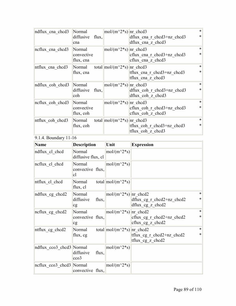
Page 89 of 110
ndflux_cna_chcd3 Normal
diffusive flux,
cna
mol/(m^2*s) nr_chcd3 *
dflux_cna_r_chcd3+nz_chcd3 *
dflux_cna_z_chcd3
ncflux_cna_chcd3 Normal
convective
flux, cna
mol/(m^2*s) nr_chcd3 *
cflux_cna_r_chcd3+nz_chcd3 *
cflux_cna_z_chcd3
ntflux_cna_chcd3 Normal total
flux, cna
mol/(m^2*s) nr_chcd3 *
tflux_cna_r_chcd3+nz_chcd3 *
tflux_cna_z_chcd3
ndflux_coh_chcd3 Normal
diffusive flux,
coh
mol/(m^2*s) nr_chcd3 *
dflux_coh_r_chcd3+nz_chcd3 *
dflux_coh_z_chcd3
ncflux_coh_chcd3 Normal
convective
flux, coh
mol/(m^2*s) nr_chcd3 *
cflux_coh_r_chcd3+nz_chcd3 *
cflux_coh_z_chcd3
ntflux_coh_chcd3 Normal total
flux, coh
mol/(m^2*s) nr_chcd3 *
tflux_coh_r_chcd3+nz_chcd3 *
tflux_coh_z_chcd3
9.1.4. Boundary 11-16
Name Description Unit Expression
ndflux_cl_chcd Normal
diffusive flux, cl
mol/(m^2*s)
ncflux_cl_chcd Normal
convective flux,
cl
mol/(m^2*s)
ntflux_cl_chcd Normal total
flux, cl
mol/(m^2*s)
ndflux_cg_chcd2 Normal
diffusive flux,
cg
mol/(m^2*s) nr_chcd2 *
dflux_cg_r_chcd2+nz_chcd2 *
dflux_cg_z_chcd2
ncflux_cg_chcd2 Normal
convective flux,
cg
mol/(m^2*s) nr_chcd2 *
cflux_cg_r_chcd2+nz_chcd2 *
cflux_cg_z_chcd2
ntflux_cg_chcd2 Normal total
flux, cg
mol/(m^2*s) nr_chcd2 *
tflux_cg_r_chcd2+nz_chcd2 *
tflux_cg_z_chcd2
ndflux_cco3_chcd3 Normal
diffusive flux,
cco3
mol/(m^2*s)
ncflux_cco3_chcd3 Normal
convective flux,
mol/(m^2*s)
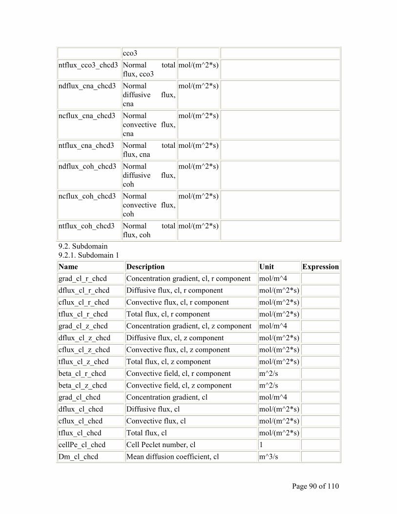
Page 90 of 110
cco3
ntflux_cco3_chcd3 Normal total
flux, cco3
mol/(m^2*s)
ndflux_cna_chcd3 Normal
diffusive flux,
cna
mol/(m^2*s)
ncflux_cna_chcd3 Normal
convective flux,
cna
mol/(m^2*s)
ntflux_cna_chcd3 Normal total
flux, cna
mol/(m^2*s)
ndflux_coh_chcd3 Normal
diffusive flux,
coh
mol/(m^2*s)
ncflux_coh_chcd3 Normal
convective flux,
coh
mol/(m^2*s)
ntflux_coh_chcd3 Normal total
flux, coh
mol/(m^2*s)
9.2. Subdomain
9.2.1. Subdomain 1
Name Description Unit Expression
grad_cl_r_chcd Concentration gradient, cl, r component mol/m^4
dflux_cl_r_chcd Diffusive flux, cl, r component mol/(m^2*s)
cflux_cl_r_chcd Convective flux, cl, r component mol/(m^2*s)
tflux_cl_r_chcd Total flux, cl, r component mol/(m^2*s)
grad_cl_z_chcd Concentration gradient, cl, z component mol/m^4
dflux_cl_z_chcd Diffusive flux, cl, z component mol/(m^2*s)
cflux_cl_z_chcd Convective flux, cl, z component mol/(m^2*s)
tflux_cl_z_chcd Total flux, cl, z component mol/(m^2*s)
beta_cl_r_chcd Convective field, cl, r component m^2/s
beta_cl_z_chcd Convective field, cl, z component m^2/s
grad_cl_chcd Concentration gradient, cl mol/m^4
dflux_cl_chcd Diffusive flux, cl mol/(m^2*s)
cflux_cl_chcd Convective flux, cl mol/(m^2*s)
tflux_cl_chcd Total flux, cl mol/(m^2*s)
cellPe_cl_chcd Cell Peclet number, cl 1
Dm_cl_chcd Mean diffusion coefficient, cl m^3/s
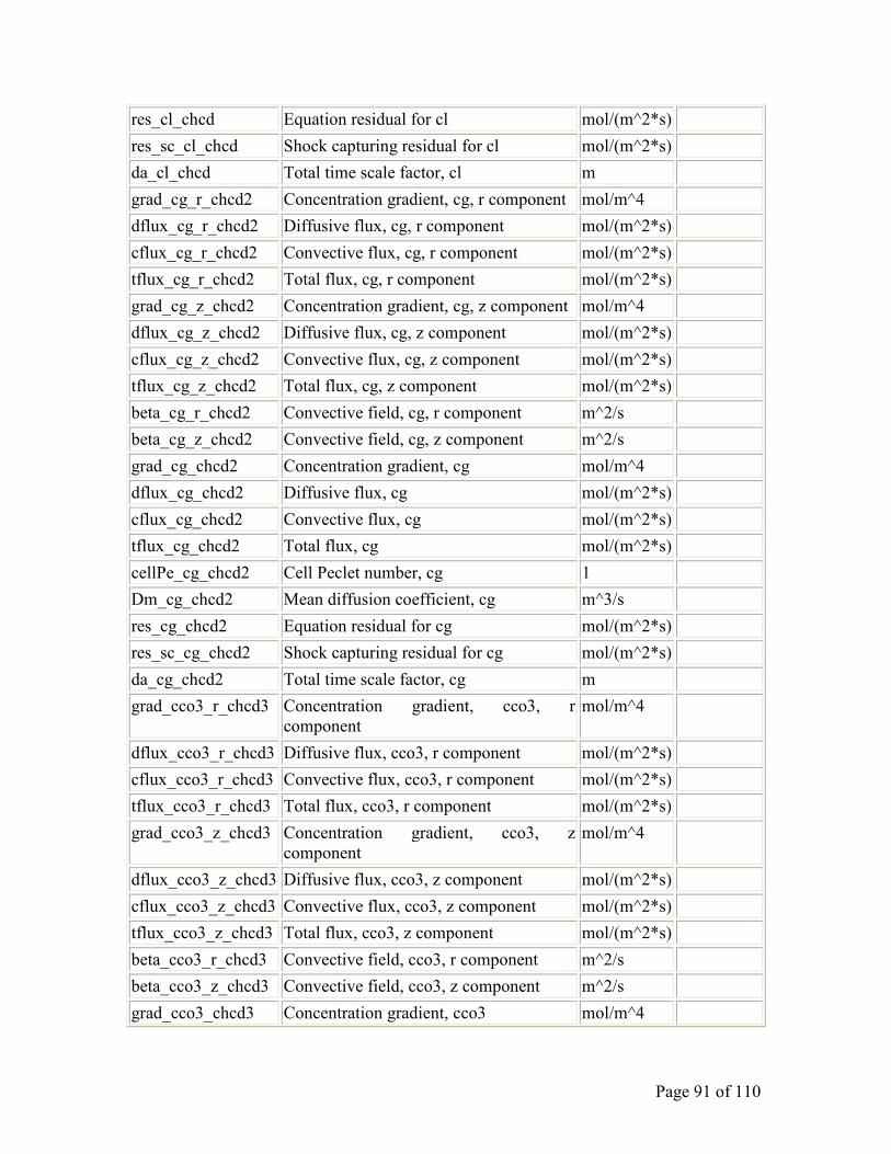
Page 91 of 110
res_cl_chcd Equation residual for cl mol/(m^2*s)
res_sc_cl_chcd Shock capturing residual for cl mol/(m^2*s)
da_cl_chcd Total time scale factor, cl m
grad_cg_r_chcd2 Concentration gradient, cg, r component mol/m^4
dflux_cg_r_chcd2 Diffusive flux, cg, r component mol/(m^2*s)
cflux_cg_r_chcd2 Convective flux, cg, r component mol/(m^2*s)
tflux_cg_r_chcd2 Total flux, cg, r component mol/(m^2*s)
grad_cg_z_chcd2 Concentration gradient, cg, z component mol/m^4
dflux_cg_z_chcd2 Diffusive flux, cg, z component mol/(m^2*s)
cflux_cg_z_chcd2 Convective flux, cg, z component mol/(m^2*s)
tflux_cg_z_chcd2 Total flux, cg, z component mol/(m^2*s)
beta_cg_r_chcd2 Convective field, cg, r component m^2/s
beta_cg_z_chcd2 Convective field, cg, z component m^2/s
grad_cg_chcd2 Concentration gradient, cg mol/m^4
dflux_cg_chcd2 Diffusive flux, cg mol/(m^2*s)
cflux_cg_chcd2 Convective flux, cg mol/(m^2*s)
tflux_cg_chcd2 Total flux, cg mol/(m^2*s)
cellPe_cg_chcd2 Cell Peclet number, cg 1
Dm_cg_chcd2 Mean diffusion coefficient, cg m^3/s
res_cg_chcd2 Equation residual for cg mol/(m^2*s)
res_sc_cg_chcd2 Shock capturing residual for cg mol/(m^2*s)
da_cg_chcd2 Total time scale factor, cg m
grad_cco3_r_chcd3 Concentration gradient, cco3, r
component
mol/m^4
dflux_cco3_r_chcd3 Diffusive flux, cco3, r component mol/(m^2*s)
cflux_cco3_r_chcd3 Convective flux, cco3, r component mol/(m^2*s)
tflux_cco3_r_chcd3 Total flux, cco3, r component mol/(m^2*s)
grad_cco3_z_chcd3 Concentration gradient, cco3, z
component
mol/m^4
dflux_cco3_z_chcd3 Diffusive flux, cco3, z component mol/(m^2*s)
cflux_cco3_z_chcd3 Convective flux, cco3, z component mol/(m^2*s)
tflux_cco3_z_chcd3 Total flux, cco3, z component mol/(m^2*s)
beta_cco3_r_chcd3 Convective field, cco3, r component m^2/s
beta_cco3_z_chcd3 Convective field, cco3, z component m^2/s
grad_cco3_chcd3 Concentration gradient, cco3 mol/m^4
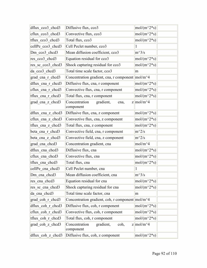
Page 92 of 110
dflux_cco3_chcd3 Diffusive flux, cco3 mol/(m^2*s)
cflux_cco3_chcd3 Convective flux, cco3 mol/(m^2*s)
tflux_cco3_chcd3 Total flux, cco3 mol/(m^2*s)
cellPe_cco3_chcd3 Cell Peclet number, cco3 1
Dm_cco3_chcd3 Mean diffusion coefficient, cco3 m^3/s
res_cco3_chcd3 Equation residual for cco3 mol/(m^2*s)
res_sc_cco3_chcd3 Shock capturing residual for cco3 mol/(m^2*s)
da_cco3_chcd3 Total time scale factor, cco3 m
grad_cna_r_chcd3 Concentration gradient, cna, r component mol/m^4
dflux_cna_r_chcd3 Diffusive flux, cna, r component mol/(m^2*s)
cflux_cna_r_chcd3 Convective flux, cna, r component mol/(m^2*s)
tflux_cna_r_chcd3 Total flux, cna, r component mol/(m^2*s)
grad_cna_z_chcd3 Concentration gradient, cna, z
component
mol/m^4
dflux_cna_z_chcd3 Diffusive flux, cna, z component mol/(m^2*s)
cflux_cna_z_chcd3 Convective flux, cna, z component mol/(m^2*s)
tflux_cna_z_chcd3 Total flux, cna, z component mol/(m^2*s)
beta_cna_r_chcd3 Convective field, cna, r component m^2/s
beta_cna_z_chcd3 Convective field, cna, z component m^2/s
grad_cna_chcd3 Concentration gradient, cna mol/m^4
dflux_cna_chcd3 Diffusive flux, cna mol/(m^2*s)
cflux_cna_chcd3 Convective flux, cna mol/(m^2*s)
tflux_cna_chcd3 Total flux, cna mol/(m^2*s)
cellPe_cna_chcd3 Cell Peclet number, cna 1
Dm_cna_chcd3 Mean diffusion coefficient, cna m^3/s
res_cna_chcd3 Equation residual for cna mol/(m^2*s)
res_sc_cna_chcd3 Shock capturing residual for cna mol/(m^2*s)
da_cna_chcd3 Total time scale factor, cna m
grad_coh_r_chcd3 Concentration gradient, coh, r component mol/m^4
dflux_coh_r_chcd3 Diffusive flux, coh, r component mol/(m^2*s)
cflux_coh_r_chcd3 Convective flux, coh, r component mol/(m^2*s)
tflux_coh_r_chcd3 Total flux, coh, r component mol/(m^2*s)
grad_coh_z_chcd3 Concentration gradient, coh, z
component
mol/m^4
dflux_coh_z_chcd3 Diffusive flux, coh, z component mol/(m^2*s)

Page 93 of 110
cflux_coh_z_chcd3 Convective flux, coh, z component mol/(m^2*s)
tflux_coh_z_chcd3 Total flux, coh, z component mol/(m^2*s)
beta_coh_r_chcd3 Convective field, coh, r component m^2/s
beta_coh_z_chcd3 Convective field, coh, z component m^2/s
grad_coh_chcd3 Concentration gradient, coh mol/m^4
dflux_coh_chcd3 Diffusive flux, coh mol/(m^2*s)
cflux_coh_chcd3 Convective flux, coh mol/(m^2*s)
tflux_coh_chcd3 Total flux, coh mol/(m^2*s)
cellPe_coh_chcd3 Cell Peclet number, coh 1
Dm_coh_chcd3 Mean diffusion coefficient, coh m^3/s
res_coh_chcd3 Equation residual for coh mol/(m^2*s)
res_sc_coh_chcd3 Shock capturing residual for coh mol/(m^2*s)
da_coh_chcd3 Total time scale factor, coh m
9.2.2. Subdomain 2-3
Name Descripti
on
Unit Expression
grad_cl_r_chcd Concentra
tion
gradient,
cl, r
componen
t
mol/m^4 clr
dflux_cl_r_chc
d
Diffusive
flux, cl, r
componen
t
mol/(m^
2*s)
-Drr_cl_chcd * clr-Drz_cl_chcd * clz
cflux_cl_r_chc
d
Convectiv
e flux, cl,
r
componen
t
mol/(m^
2*s)
cl * u_cl_chcd
tflux_cl_r_chc
d
Total flux,
cl, r
componen
t
mol/(m^
2*s)
dflux_cl_r_chcd+cflux_cl_r_chcd
grad_cl_z_chc
d
Concentra
tion
gradient,
cl, z
componen
mol/m^4 clz
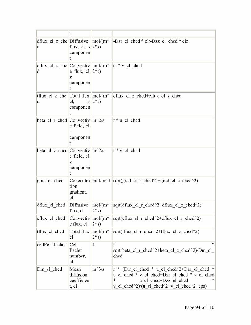
Page 94 of 110
t
dflux_cl_z_chc
d
Diffusive
flux, cl, z
componen
t
mol/(m^
2*s)
-Dzr_cl_chcd * clr-Dzz_cl_chcd * clz
cflux_cl_z_chc
d
Convectiv
e flux, cl,
z
componen
t
mol/(m^
2*s)
cl * v_cl_chcd
tflux_cl_z_chc
d
Total flux,
cl, z
componen
t
mol/(m^
2*s)
dflux_cl_z_chcd+cflux_cl_z_chcd
beta_cl_r_chcd Convectiv
e field, cl,
r
componen
t
m^2/s r * u_cl_chcd
beta_cl_z_chcd Convectiv
e field, cl,
z
componen
t
m^2/s r * v_cl_chcd
grad_cl_chcd Concentra
tion
gradient,
cl
mol/m^4 sqrt(grad_cl_r_chcd^2+grad_cl_z_chcd^2)
dflux_cl_chcd Diffusive
flux, cl
mol/(m^
2*s)
sqrt(dflux_cl_r_chcd^2+dflux_cl_z_chcd^2)
cflux_cl_chcd Convectiv
e flux, cl
mol/(m^
2*s)
sqrt(cflux_cl_r_chcd^2+cflux_cl_z_chcd^2)
tflux_cl_chcd Total flux,
cl
mol/(m^
2*s)
sqrt(tflux_cl_r_chcd^2+tflux_cl_z_chcd^2)
cellPe_cl_chcd Cell
Peclet
number,
cl
1 h *
sqrt(beta_cl_r_chcd^2+beta_cl_z_chcd^2)/Dm_cl_
chcd
Dm_cl_chcd Mean
diffusion
coefficien
t, cl
m^3/s r * (Drr_cl_chcd * u_cl_chcd^2+Drz_cl_chcd *
u_cl_chcd * v_cl_chcd+Dzr_cl_chcd * v_cl_chcd
* u_cl_chcd+Dzz_cl_chcd *
v_cl_chcd^2)/(u_cl_chcd^2+v_cl_chcd^2+eps)
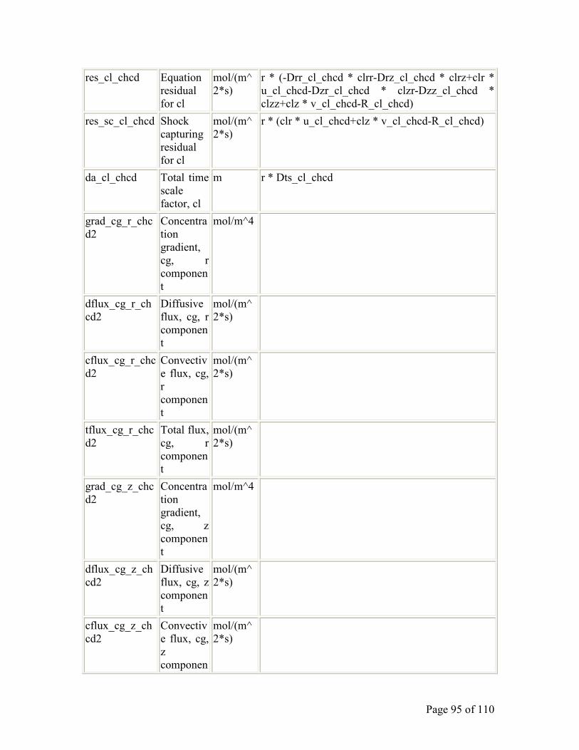
Page 95 of 110
res_cl_chcd Equation
residual
for cl
mol/(m^
2*s)
r * (-Drr_cl_chcd * clrr-Drz_cl_chcd * clrz+clr *
u_cl_chcd-Dzr_cl_chcd * clzr-Dzz_cl_chcd *
clzz+clz * v_cl_chcd-R_cl_chcd)
res_sc_cl_chcd Shock
capturing
residual
for cl
mol/(m^
2*s)
r * (clr * u_cl_chcd+clz * v_cl_chcd-R_cl_chcd)
da_cl_chcd Total time
scale
factor, cl
m r * Dts_cl_chcd
grad_cg_r_chc
d2
Concentra
tion
gradient,
cg, r
componen
t
mol/m^4
dflux_cg_r_ch
cd2
Diffusive
flux, cg, r
componen
t
mol/(m^
2*s)
cflux_cg_r_chc
d2
Convectiv
e flux, cg,
r
componen
t
mol/(m^
2*s)
tflux_cg_r_chc
d2
Total flux,
cg, r
componen
t
mol/(m^
2*s)
grad_cg_z_chc
d2
Concentra
tion
gradient,
cg, z
componen
t
mol/m^4
dflux_cg_z_ch
cd2
Diffusive
flux, cg, z
componen
t
mol/(m^
2*s)
cflux_cg_z_ch
cd2
Convectiv
e flux, cg,
z
componen
mol/(m^
2*s)
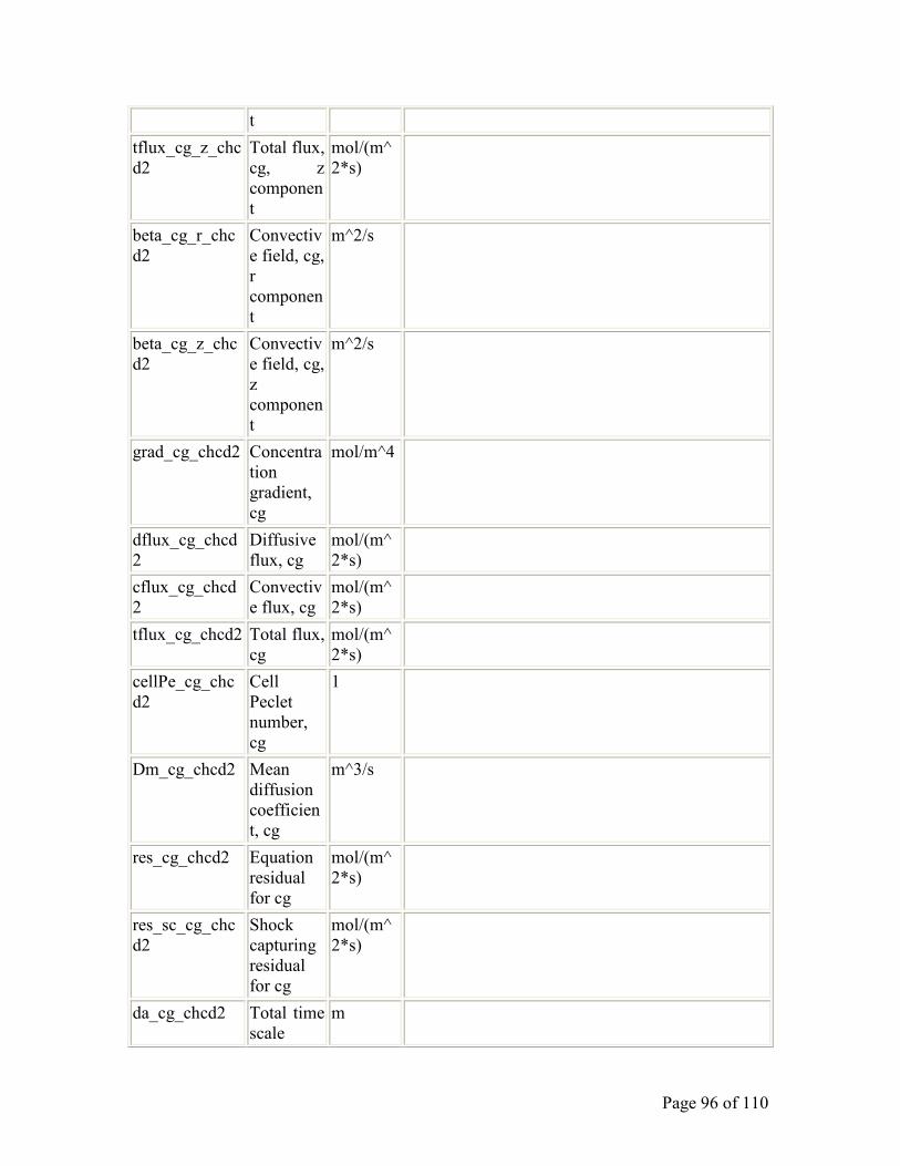
Page 96 of 110
t
tflux_cg_z_chc
d2
Total flux,
cg, z
componen
t
mol/(m^
2*s)
beta_cg_r_chc
d2
Convectiv
e field, cg,
r
componen
t
m^2/s
beta_cg_z_chc
d2
Convectiv
e field, cg,
z
componen
t
m^2/s
grad_cg_chcd2 Concentra
tion
gradient,
cg
mol/m^4
dflux_cg_chcd
2
Diffusive
flux, cg
mol/(m^
2*s)
cflux_cg_chcd
2
Convectiv
e flux, cg
mol/(m^
2*s)
tflux_cg_chcd2 Total flux,
cg
mol/(m^
2*s)
cellPe_cg_chc
d2
Cell
Peclet
number,
cg
1
Dm_cg_chcd2 Mean
diffusion
coefficien
t, cg
m^3/s
res_cg_chcd2 Equation
residual
for cg
mol/(m^
2*s)
res_sc_cg_chc
d2
Shock
capturing
residual
for cg
mol/(m^
2*s)
da_cg_chcd2 Total time
scale
m
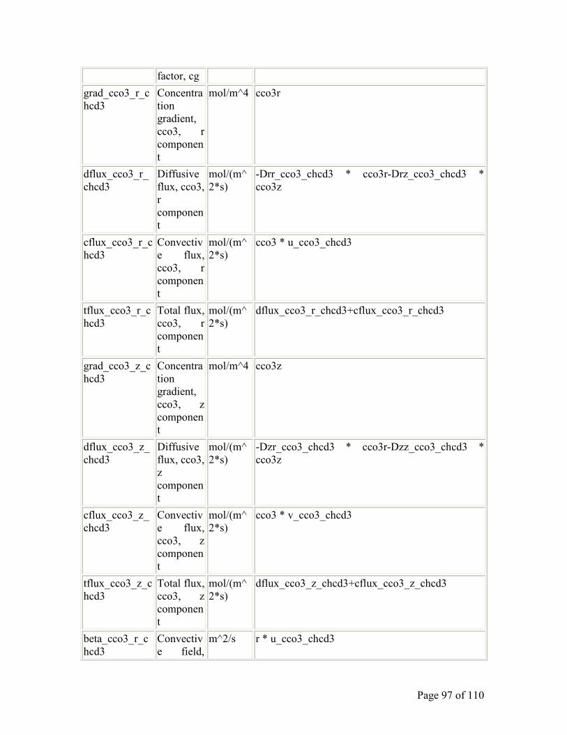
Page 97 of 110
factor, cg
grad_cco3_r_c
hcd3
Concentra
tion
gradient,
cco3, r
componen
t
mol/m^4 cco3r
dflux_cco3_r_
chcd3
Diffusive
flux, cco3,
r
componen
t
mol/(m^
2*s)
-Drr_cco3_chcd3 * cco3r-Drz_cco3_chcd3 *
cco3z
cflux_cco3_r_c
hcd3
Convectiv
e flux,
cco3, r
componen
t
mol/(m^
2*s)
cco3 * u_cco3_chcd3
tflux_cco3_r_c
hcd3
Total flux,
cco3, r
componen
t
mol/(m^
2*s)
dflux_cco3_r_chcd3+cflux_cco3_r_chcd3
grad_cco3_z_c
hcd3
Concentra
tion
gradient,
cco3, z
componen
t
mol/m^4 cco3z
dflux_cco3_z_
chcd3
Diffusive
flux, cco3,
z
componen
t
mol/(m^
2*s)
-Dzr_cco3_chcd3 * cco3r-Dzz_cco3_chcd3 *
cco3z
cflux_cco3_z_
chcd3
Convectiv
e flux,
cco3, z
componen
t
mol/(m^
2*s)
cco3 * v_cco3_chcd3
tflux_cco3_z_c
hcd3
Total flux,
cco3, z
componen
t
mol/(m^
2*s)
dflux_cco3_z_chcd3+cflux_cco3_z_chcd3
beta_cco3_r_c
hcd3
Convectiv
e field,
m^2/s r * u_cco3_chcd3

Page 98 of 110
cco3, r
componen
t
beta_cco3_z_c
hcd3
Convectiv
e field,
cco3, z
componen
t
m^2/s r * v_cco3_chcd3
grad_cco3_chc
d3
Concentra
tion
gradient,
cco3
mol/m^4 sqrt(grad_cco3_r_chcd3^2+grad_cco3_z_chcd3^2
)
dflux_cco3_ch
cd3
Diffusive
flux, cco3
mol/(m^
2*s)
sqrt(dflux_cco3_r_chcd3^2+dflux_cco3_z_chcd3^
2)
cflux_cco3_ch
cd3
Convectiv
e flux,
cco3
mol/(m^
2*s)
sqrt(cflux_cco3_r_chcd3^2+cflux_cco3_z_chcd3^
2)
tflux_cco3_chc
d3
Total flux,
cco3
mol/(m^
2*s)
sqrt(tflux_cco3_r_chcd3^2+tflux_cco3_z_chcd3^2
)
cellPe_cco3_c
hcd3
Cell
Peclet
number,
cco3
1 h *
sqrt(beta_cco3_r_chcd3^2+beta_cco3_z_chcd3^2)
/Dm_cco3_chcd3
Dm_cco3_chc
d3
Mean
diffusion
coefficien
t, cco3
m^3/s r * (Drr_cco3_chcd3 *
u_cco3_chcd3^2+Drz_cco3_chcd3 *
u_cco3_chcd3 * v_cco3_chcd3+Dzr_cco3_chcd3
* v_cco3_chcd3 *
u_cco3_chcd3+Dzz_cco3_chcd3 *
v_cco3_chcd3^2)/(u_cco3_chcd3^2+v_cco3_chcd
3^2+eps)
res_cco3_chcd
3
Equation
residual
for cco3
mol/(m^
2*s)
r * (-Drr_cco3_chcd3 * cco3rr-Drz_cco3_chcd3 *
cco3rz+cco3r * u_cco3_chcd3-Dzr_cco3_chcd3 *
cco3zr-Dzz_cco3_chcd3 * cco3zz+cco3z *
v_cco3_chcd3-R_cco3_chcd3)
res_sc_cco3_c
hcd3
Shock
capturing
residual
for cco3
mol/(m^
2*s)
r * (cco3r * u_cco3_chcd3+cco3z *
v_cco3_chcd3-R_cco3_chcd3)
da_cco3_chcd3 Total time
scale
factor,
cco3
m r * Dts_cco3_chcd3

Page 99 of 110
grad_cna_r_ch
cd3
Concentra
tion
gradient,
cna, r
componen
t
mol/m^4 cnar
dflux_cna_r_c
hcd3
Diffusive
flux, cna,
r
componen
t
mol/(m^
2*s)
-Drr_cna_chcd3 * cnar-Drz_cna_chcd3 * cnaz
cflux_cna_r_ch
cd3
Convectiv
e flux,
cna, r
componen
t
mol/(m^
2*s)
cna * u_cna_chcd3
tflux_cna_r_ch
cd3
Total flux,
cna, r
componen
t
mol/(m^
2*s)
dflux_cna_r_chcd3+cflux_cna_r_chcd3
grad_cna_z_ch
cd3
Concentra
tion
gradient,
cna, z
componen
t
mol/m^4 cnaz
dflux_cna_z_c
hcd3
Diffusive
flux, cna,
z
componen
t
mol/(m^
2*s)
-Dzr_cna_chcd3 * cnar-Dzz_cna_chcd3 * cnaz
cflux_cna_z_c
hcd3
Convectiv
e flux,
cna, z
componen
t
mol/(m^
2*s)
cna * v_cna_chcd3
tflux_cna_z_ch
cd3
Total flux,
cna, z
componen
t
mol/(m^
2*s)
dflux_cna_z_chcd3+cflux_cna_z_chcd3
beta_cna_r_ch
cd3
Convectiv
e field,
cna, r
m^2/s r * u_cna_chcd3

Page 100 of 110
componen
t
beta_cna_z_ch
cd3
Convectiv
e field,
cna, z
componen
t
m^2/s r * v_cna_chcd3
grad_cna_chcd
3
Concentra
tion
gradient,
cna
mol/m^4 sqrt(grad_cna_r_chcd3^2+grad_cna_z_chcd3^2)
dflux_cna_chc
d3
Diffusive
flux, cna
mol/(m^
2*s)
sqrt(dflux_cna_r_chcd3^2+dflux_cna_z_chcd3^2)
cflux_cna_chc
d3
Convectiv
e flux, cna
mol/(m^
2*s)
sqrt(cflux_cna_r_chcd3^2+cflux_cna_z_chcd3^2)
tflux_cna_chcd
3
Total flux,
cna
mol/(m^
2*s)
sqrt(tflux_cna_r_chcd3^2+tflux_cna_z_chcd3^2)
cellPe_cna_chc
d3
Cell
Peclet
number,
cna
1 h *
sqrt(beta_cna_r_chcd3^2+beta_cna_z_chcd3^2)/D
m_cna_chcd3
Dm_cna_chcd
3
Mean
diffusion
coefficien
t, cna
m^3/s r * (Drr_cna_chcd3 *
u_cna_chcd3^2+Drz_cna_chcd3 * u_cna_chcd3 *
v_cna_chcd3+Dzr_cna_chcd3 * v_cna_chcd3 *
u_cna_chcd3+Dzz_cna_chcd3 *
v_cna_chcd3^2)/(u_cna_chcd3^2+v_cna_chcd3^2
+eps)
res_cna_chcd3 Equation
residual
for cna
mol/(m^
2*s)
r * (-Drr_cna_chcd3 * cnarr-Drz_cna_chcd3 *
cnarz+cnar * u_cna_chcd3-Dzr_cna_chcd3 *
cnazr-Dzz_cna_chcd3 * cnazz+cnaz *
v_cna_chcd3-R_cna_chcd3)
res_sc_cna_ch
cd3
Shock
capturing
residual
for cna
mol/(m^
2*s)
r * (cnar * u_cna_chcd3+cnaz * v_cna_chcd3-
R_cna_chcd3)
da_cna_chcd3 Total time
scale
factor, cna
m r * Dts_cna_chcd3
grad_coh_r_ch
cd3
Concentra
tion
gradient,
coh, r
mol/m^4 cohr
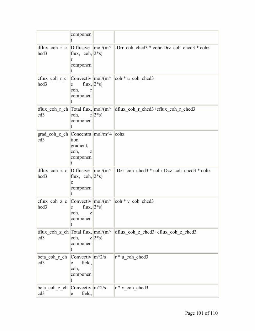
Page 101 of 110
componen
t
dflux_coh_r_c
hcd3
Diffusive
flux, coh,
r
componen
t
mol/(m^
2*s)
-Drr_coh_chcd3 * cohr-Drz_coh_chcd3 * cohz
cflux_coh_r_c
hcd3
Convectiv
e flux,
coh, r
componen
t
mol/(m^
2*s)
coh * u_coh_chcd3
tflux_coh_r_ch
cd3
Total flux,
coh, r
componen
t
mol/(m^
2*s)
dflux_coh_r_chcd3+cflux_coh_r_chcd3
grad_coh_z_ch
cd3
Concentra
tion
gradient,
coh, z
componen
t
mol/m^4 cohz
dflux_coh_z_c
hcd3
Diffusive
flux, coh,
z
componen
t
mol/(m^
2*s)
-Dzr_coh_chcd3 * cohr-Dzz_coh_chcd3 * cohz
cflux_coh_z_c
hcd3
Convectiv
e flux,
coh, z
componen
t
mol/(m^
2*s)
coh * v_coh_chcd3
tflux_coh_z_ch
cd3
Total flux,
coh, z
componen
t
mol/(m^
2*s)
dflux_coh_z_chcd3+cflux_coh_z_chcd3
beta_coh_r_ch
cd3
Convectiv
e field,
coh, r
componen
t
m^2/s r * u_coh_chcd3
beta_coh_z_ch
cd3
Convectiv
e field,
m^2/s r * v_coh_chcd3
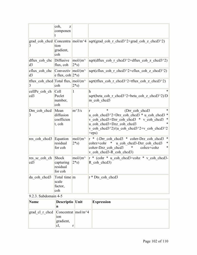
Page 102 of 110
coh, z
componen
t
grad_coh_chcd
3
Concentra
tion
gradient,
coh
mol/m^4 sqrt(grad_coh_r_chcd3^2+grad_coh_z_chcd3^2)
dflux_coh_chc
d3
Diffusive
flux, coh
mol/(m^
2*s)
sqrt(dflux_coh_r_chcd3^2+dflux_coh_z_chcd3^2)
cflux_coh_chc
d3
Convectiv
e flux, coh
mol/(m^
2*s)
sqrt(cflux_coh_r_chcd3^2+cflux_coh_z_chcd3^2)
tflux_coh_chcd
3
Total flux,
coh
mol/(m^
2*s)
sqrt(tflux_coh_r_chcd3^2+tflux_coh_z_chcd3^2)
cellPe_coh_ch
cd3
Cell
Peclet
number,
coh
1 h *
sqrt(beta_coh_r_chcd3^2+beta_coh_z_chcd3^2)/D
m_coh_chcd3
Dm_coh_chcd
3
Mean
diffusion
coefficien
t, coh
m^3/s r * (Drr_coh_chcd3 *
u_coh_chcd3^2+Drz_coh_chcd3 * u_coh_chcd3 *
v_coh_chcd3+Dzr_coh_chcd3 * v_coh_chcd3 *
u_coh_chcd3+Dzz_coh_chcd3 *
v_coh_chcd3^2)/(u_coh_chcd3^2+v_coh_chcd3^2
+eps)
res_coh_chcd3 Equation
residual
for coh
mol/(m^
2*s)
r * (-Drr_coh_chcd3 * cohrr-Drz_coh_chcd3 *
cohrz+cohr * u_coh_chcd3-Dzr_coh_chcd3 *
cohzr-Dzz_coh_chcd3 * cohzz+cohz *
v_coh_chcd3-R_coh_chcd3)
res_sc_coh_ch
cd3
Shock
capturing
residual
for coh
mol/(m^
2*s)
r * (cohr * u_coh_chcd3+cohz * v_coh_chcd3-
R_coh_chcd3)
da_coh_chcd3 Total time
scale
factor,
coh
m r * Dts_coh_chcd3
9.2.3. Subdomain 4-5
Name Descriptio
n
Unit Expression
grad_cl_r_chcd Concentrat
ion
gradient,
cl, r
mol/m^4

Page 103 of 110
component
dflux_cl_r_chcd Diffusive
flux, cl, r
component
mol/(m^2
*s)
cflux_cl_r_chcd Convectiv
e flux, cl, r
component
mol/(m^2
*s)
tflux_cl_r_chcd Total flux,
cl, r
component
mol/(m^2
*s)
grad_cl_z_chcd Concentrat
ion
gradient,
cl, z
component
mol/m^4
dflux_cl_z_chc
d
Diffusive
flux, cl, z
component
mol/(m^2
*s)
cflux_cl_z_chcd Convectiv
e flux, cl, z
component
mol/(m^2
*s)
tflux_cl_z_chcd Total flux,
cl, z
component
mol/(m^2
*s)
beta_cl_r_chcd Convectiv
e field, cl,
r
component
m^2/s
beta_cl_z_chcd Convectiv
e field, cl,
z
component
m^2/s
grad_cl_chcd Concentrat
ion
gradient, cl
mol/m^4
dflux_cl_chcd Diffusive
flux, cl
mol/(m^2
*s)
cflux_cl_chcd Convectiv
e flux, cl
mol/(m^2
*s)
tflux_cl_chcd Total flux,
cl
mol/(m^2
*s)
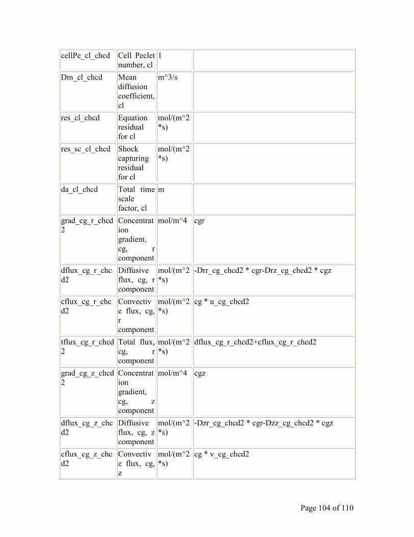
Page 104 of 110
cellPe_cl_chcd Cell Peclet
number, cl
1
Dm_cl_chcd Mean
diffusion
coefficient,
cl
m^3/s
res_cl_chcd Equation
residual
for cl
mol/(m^2
*s)
res_sc_cl_chcd Shock
capturing
residual
for cl
mol/(m^2
*s)
da_cl_chcd Total time
scale
factor, cl
m
grad_cg_r_chcd
2
Concentrat
ion
gradient,
cg, r
component
mol/m^4 cgr
dflux_cg_r_chc
d2
Diffusive
flux, cg, r
component
mol/(m^2
*s)
-Drr_cg_chcd2 * cgr-Drz_cg_chcd2 * cgz
cflux_cg_r_chc
d2
Convectiv
e flux, cg,
r
component
mol/(m^2
*s)
cg * u_cg_chcd2
tflux_cg_r_chcd
2
Total flux,
cg, r
component
mol/(m^2
*s)
dflux_cg_r_chcd2+cflux_cg_r_chcd2
grad_cg_z_chcd
2
Concentrat
ion
gradient,
cg, z
component
mol/m^4 cgz
dflux_cg_z_chc
d2
Diffusive
flux, cg, z
component
mol/(m^2
*s)
-Dzr_cg_chcd2 * cgr-Dzz_cg_chcd2 * cgz
cflux_cg_z_chc
d2
Convectiv
e flux, cg,
z
mol/(m^2
*s)
cg * v_cg_chcd2

Page 105 of 110
component
tflux_cg_z_chc
d2
Total flux,
cg, z
component
mol/(m^2
*s)
dflux_cg_z_chcd2+cflux_cg_z_chcd2
beta_cg_r_chcd
2
Convectiv
e field, cg,
r
component
m^2/s r * u_cg_chcd2
beta_cg_z_chcd
2
Convectiv
e field, cg,
z
component
m^2/s r * v_cg_chcd2
grad_cg_chcd2 Concentrat
ion
gradient,
cg
mol/m^4 sqrt(grad_cg_r_chcd2^2+grad_cg_z_chcd2^2)
dflux_cg_chcd2 Diffusive
flux, cg
mol/(m^2
*s)
sqrt(dflux_cg_r_chcd2^2+dflux_cg_z_chcd2^2)
cflux_cg_chcd2 Convectiv
e flux, cg
mol/(m^2
*s)
sqrt(cflux_cg_r_chcd2^2+cflux_cg_z_chcd2^2)
tflux_cg_chcd2 Total flux,
cg
mol/(m^2
*s)
sqrt(tflux_cg_r_chcd2^2+tflux_cg_z_chcd2^2)
cellPe_cg_chcd
2
Cell Peclet
number, cg
1 h *
sqrt(beta_cg_r_chcd2^2+beta_cg_z_chcd2^2)/D
m_cg_chcd2
Dm_cg_chcd2 Mean
diffusion
coefficient,
cg
m^3/s r * (Drr_cg_chcd2 *
u_cg_chcd2^2+Drz_cg_chcd2 * u_cg_chcd2 *
v_cg_chcd2+Dzr_cg_chcd2 * v_cg_chcd2 *
u_cg_chcd2+Dzz_cg_chcd2 *
v_cg_chcd2^2)/(u_cg_chcd2^2+v_cg_chcd2^2+
eps)
res_cg_chcd2 Equation
residual
for cg
mol/(m^2
*s)
r * (-Drr_cg_chcd2 * cgrr-Drz_cg_chcd2 *
cgrz+cgr * u_cg_chcd2-Dzr_cg_chcd2 * cgzr-
Dzz_cg_chcd2 * cgzz+cgz * v_cg_chcd2-
R_cg_chcd2)
res_sc_cg_chcd
2
Shock
capturing
residual
for cg
mol/(m^2
*s)
r * (cgr * u_cg_chcd2+cgz * v_cg_chcd2-
R_cg_chcd2)
da_cg_chcd2 Total time
scale
factor, cg
m r * Dts_cg_chcd2

Page 106 of 110
grad_cco3_r_ch
cd3
Concentrat
ion
gradient,
cco3, r
component
mol/m^4
dflux_cco3_r_c
hcd3
Diffusive
flux, cco3,
r
component
mol/(m^2
*s)
cflux_cco3_r_c
hcd3
Convectiv
e flux,
cco3, r
component
mol/(m^2
*s)
tflux_cco3_r_ch
cd3
Total flux,
cco3, r
component
mol/(m^2
*s)
grad_cco3_z_ch
cd3
Concentrat
ion
gradient,
cco3, z
component
mol/m^4
dflux_cco3_z_c
hcd3
Diffusive
flux, cco3,
z
component
mol/(m^2
*s)
cflux_cco3_z_c
hcd3
Convectiv
e flux,
cco3, z
component
mol/(m^2
*s)
tflux_cco3_z_c
hcd3
Total flux,
cco3, z
component
mol/(m^2
*s)
beta_cco3_r_ch
cd3
Convectiv
e field,
cco3, r
component
m^2/s
beta_cco3_z_ch
cd3
Convectiv
e field,
cco3, z
component
m^2/s
grad_cco3_chcd
3
Concentrat
ion
gradient,
mol/m^4
Page 107 of 110
cco3
dflux_cco3_chc
d3
Diffusive
flux, cco3
mol/(m^2
*s)
cflux_cco3_chc
d3
Convectiv
e flux,
cco3
mol/(m^2
*s)
tflux_cco3_chc
d3
Total flux,
cco3
mol/(m^2
*s)
cellPe_cco3_ch
cd3
Cell Peclet
number,
cco3
1
Dm_cco3_chcd
3
Mean
diffusion
coefficient,
cco3
m^3/s
res_cco3_chcd3 Equation
residual
for cco3
mol/(m^2
*s)
res_sc_cco3_ch
cd3
Shock
capturing
residual
for cco3
mol/(m^2
*s)
da_cco3_chcd3 Total time
scale
factor,
cco3
m
grad_cna_r_chc
d3
Concentrat
ion
gradient,
cna, r
component
mol/m^4
dflux_cna_r_ch
cd3
Diffusive
flux, cna, r
component
mol/(m^2
*s)
cflux_cna_r_ch
cd3
Convectiv
e flux, cna,
r
component
mol/(m^2
*s)
tflux_cna_r_chc
d3
Total flux,
cna, r
component
mol/(m^2
*s)
grad_cna_z_chc Concentrat mol/m^4
Page 108 of 110
d3 ion
gradient,
cna, z
component
dflux_cna_z_ch
cd3
Diffusive
flux, cna, z
component
mol/(m^2
*s)
cflux_cna_z_ch
cd3
Convectiv
e flux, cna,
z
component
mol/(m^2
*s)
tflux_cna_z_chc
d3
Total flux,
cna, z
component
mol/(m^2
*s)
beta_cna_r_chc
d3
Convectiv
e field,
cna, r
component
m^2/s
beta_cna_z_chc
d3
Convectiv
e field,
cna, z
component
m^2/s
grad_cna_chcd3 Concentrat
ion
gradient,
cna
mol/m^4
dflux_cna_chcd
3
Diffusive
flux, cna
mol/(m^2
*s)
cflux_cna_chcd
3
Convectiv
e flux, cna
mol/(m^2
*s)
tflux_cna_chcd
3
Total flux,
cna
mol/(m^2
*s)
cellPe_cna_chc
d3
Cell Peclet
number,
cna
1
Dm_cna_chcd3 Mean
diffusion
coefficient,
cna
m^3/s
res_cna_chcd3 Equation
residual
for cna
mol/(m^2
*s)
Page 109 of 110
res_sc_cna_chc
d3
Shock
capturing
residual
for cna
mol/(m^2
*s)
da_cna_chcd3 Total time
scale
factor, cna
m
grad_coh_r_chc
d3
Concentrat
ion
gradient,
coh, r
component
mol/m^4
dflux_coh_r_ch
cd3
Diffusive
flux, coh, r
component
mol/(m^2
*s)
cflux_coh_r_ch
cd3
Convectiv
e flux, coh,
r
component
mol/(m^2
*s)
tflux_coh_r_chc
d3
Total flux,
coh, r
component
mol/(m^2
*s)
grad_coh_z_chc
d3
Concentrat
ion
gradient,
coh, z
component
mol/m^4
dflux_coh_z_ch
cd3
Diffusive
flux, coh, z
component
mol/(m^2
*s)
cflux_coh_z_ch
cd3
Convectiv
e flux, coh,
z
component
mol/(m^2
*s)
tflux_coh_z_ch
cd3
Total flux,
coh, z
component
mol/(m^2
*s)
beta_coh_r_chc
d3
Convectiv
e field,
coh, r
component
m^2/s
beta_coh_z_chc Convectiv m^2/s
Page 110 of 110
d3 e field,
coh, z
component
grad_coh_chcd3 Concentrat
ion
gradient,
coh
mol/m^4
dflux_coh_chcd
3
Diffusive
flux, coh
mol/(m^2
*s)
cflux_coh_chcd
3
Convectiv
e flux, coh
mol/(m^2
*s)
tflux_coh_chcd
3
Total flux,
coh
mol/(m^2
*s)
cellPe_coh_chc
d3
Cell Peclet
number,
coh
1
Dm_coh_chcd3 Mean
diffusion
coefficient,
coh
m^3/s
res_coh_chcd3 Equation
residual
for coh
mol/(m^2
*s)
res_sc_coh_chc
d3
Shock
capturing
residual
for coh
mol/(m^2
*s)
da_coh_chcd3 Total time
scale
factor, coh
m