DI

SC

US

SI

ON

P

AP

ER

S

ER

IE

S

Forschungsinstitut zur Zukunft der ArbeitInstitute for the Study of Labor

Educational Policies and Income Inequality

IZA DP No. 8222

May 2014

Daniele ChecchiHerman G. van de Werfhorst

Educational Policies and Income Inequality

Daniele Checchi University of Milan

and IZA

Herman G. van de Werfhorst University of Amsterdam

Discussion Paper No. 8222 May 2014

IZA

P.O. Box 7240 53072 Bonn

Germany

Phone: +49-228-3894-0 Fax: +49-228-3894-180

E-mail: iza@iza.org

Any opinions expressed here are those of the author(s) and not those of IZA. Research published in this series may include views on policy, but the institute itself takes no institutional policy positions. The IZA research network is committed to the IZA Guiding Principles of Research Integrity. The Institute for the Study of Labor (IZA) in Bonn is a local and virtual international research center and a place of communication between science, politics and business. IZA is an independent nonprofit organization supported by Deutsche Post Foundation. The center is associated with the University of Bonn and offers a stimulating research environment through its international network, workshops and conferences, data service, project support, research visits and doctoral program. IZA engages in (i) original and internationally competitive research in all fields of labor economics, (ii) development of policy concepts, and (iii) dissemination of research results and concepts to the interested public. IZA Discussion Papers often represent preliminary work and are circulated to encourage discussion. Citation of such a paper should account for its provisional character. A revised version may be available directly from the author.

IZA Discussion Paper No. 8222 May 2014

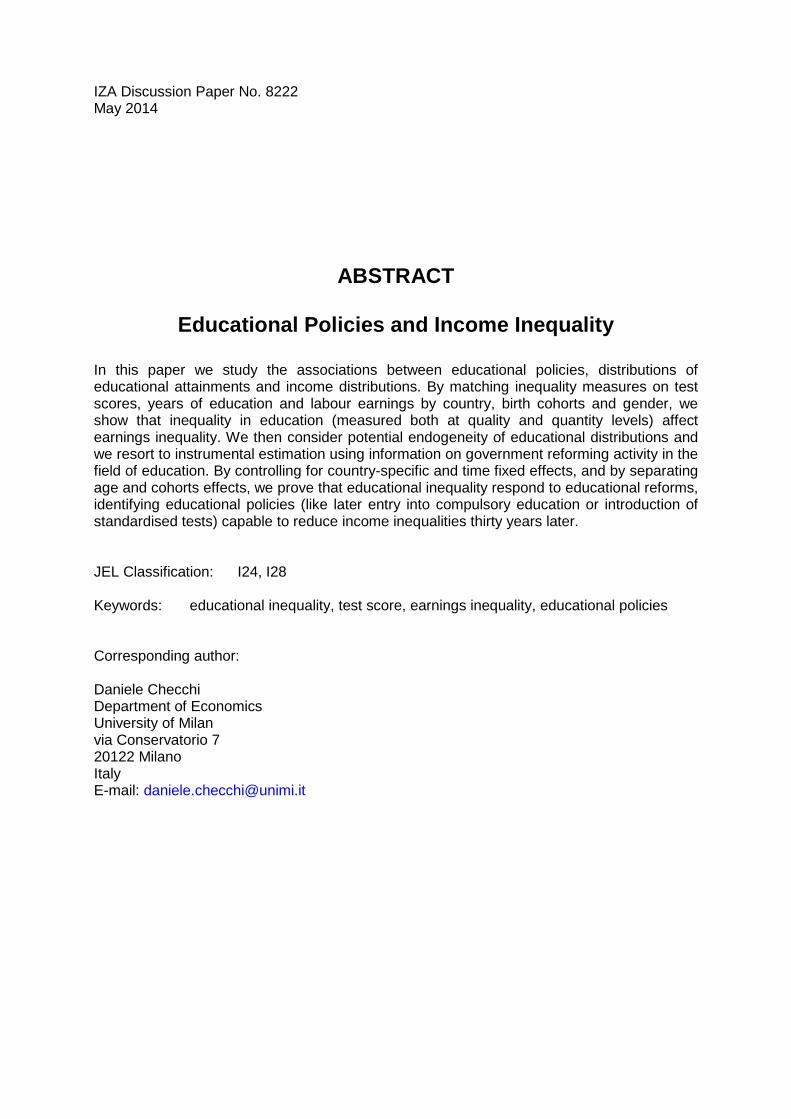
ABSTRACT

Educational Policies and Income Inequality In this paper we study the associations between educational policies, distributions of educational attainments and income distributions. By matching inequality measures on test scores, years of education and labour earnings by country, birth cohorts and gender, we show that inequality in education (measured both at quality and quantity levels) affect earnings inequality. We then consider potential endogeneity of educational distributions and we resort to instrumental estimation using information on government reforming activity in the field of education. By controlling for country-specific and time fixed effects, and by separating age and cohorts effects, we prove that educational inequality respond to educational reforms, identifying educational policies (like later entry into compulsory education or introduction of standardised tests) capable to reduce income inequalities thirty years later. JEL Classification: I24, I28 Keywords: educational inequality, test score, earnings inequality, educational policies Corresponding author: Daniele Checchi Department of Economics University of Milan via Conservatorio 7 20122 Milano Italy E-mail: daniele.checchi@unimi.it

2

Introduction

Thanks to the abundant availability of comparative data on student achievement, we have

come to know a lot about the association between characteristics of educational systems and student

learning. Student achievement tests like the Programme of International Student Assessment

(PISA), the Trends in International Mathematics and Science Study (TIMSS) and the Programme

for International Reading and Literacy Study (PIRLS) have helped us to understand whether

educational policies are related to the distribution of student performance, and inequality in

performance by social and ethnic background (Hanushek and Wössmann 2011; Kerckhoff 1995;

Van de Werfhorst and Mijs 2010; Brunello and Checchi 2007; Marks 2005; Cobb-Clark et al.

2012). Educational policies that received attention include, among others, tracking, accountability

regulations, and length of compulsory schooling.

However, there are three shortcomings in the present literature. First, most of the studies

have looked at educational policies in a static way, whereas policies in fact change over time within

countries. Given the cross-sectional nature of the comparative datasets the cross-sectional focus is

understandable, but to assess whether policies affect outcomes (in a causal meaning) one would also

want to exploit within-country temporal variations. Second, the literature has mostly concentrated

on student achievement at a relatively young age (mostly students aged between 8 and 15). Other

outcomes in educational distributions, most notably the attained level of education, has received far

less attention from a policy perspective. In other words, most attention has been paid to the ‘quality’

of education rather than its ‘quantity’. This is unfortunate, because we do not know whether policies

that are related to the quality of education are also related to the quantity of schooling in societies.

Thirdly, studies focusing on educational policy have mostly addressed educational outcomes. It is

heavily understudied whether educational policies have, through their effects on educational

distributions, also repercussions on income and earnings distributions in societies. In our view it is

crucial to understand whether policies affect educational and income distributions, because the

effectiveness of educational systems may be assessed not only in terms of the skills and

qualifications that are produced, but also in terms of the stratification in society that is generated

through educational policies. After all, educational policy is often geared towards preparing youth

for adult life, so to understand whether this preparation is successful one needs to study

distributions in earnings and income in addition to distributions in educational outcomes.

In this paper we contribute to understanding the associations between educational policies,

educational distributions and income distributions by combining four sorts of data. First, as a

starting point we have exploited comparative mathematics achievement data from various years: the

First International Mathematics Study of 1964 (FIMS64), the Second International Mathematics

3

Study of 1980-1982 (SIMS80), and the Trends in International Mathematics and Science Study of

1995 (TIMSS95). This collection provides us with mathematics achievement data, as indicator of

the ‘quality’ of education, for a multitude of cohorts and countries, split out by gender. Second, for

the cohorts and countries for which data were available in these student achievement tests, we have

collected data on educational policies, including policies on compulsory education, school and/or

teachers’ autonomy, and tracking age (see Braga et al. 2013). Third, using data from Eurostat, we

have collected data on educational attainments measured by the (median) years of schooling

required to attain a specific degree, following the ISCED classification. This is again done for each

combination of cohort, country and gender separately. Fourth, for each combination of country,

cohort and gender we have calculated income inequalities using the European Community

Household Panel (ECHP) and the European Union Statistics on Income and Living Conditions

(EUSILC), the latter being official European Union data on income statistics.

These four data sources enable us to study whether educational policies are related to the

distribution of quality and quantity of education, and whether policies and educational distributions

(of both quality and quantity) are related to income inequality. By controlling for country-specific

and time fixed effects, and by separating age and cohorts effects, we believe that our assessment of

policy effects is stronger than in most other studies. Our results indicate that inequality in education

(measured both at quality and quantity levels) affect earnings inequality. In addition, since

educational inequality respond to educational reforms, we are able to identify educational policies

(like later entry into compulsory education or introduction of standardised tests) capable to reduce

income inequalities thirty years later.

Policies, education and income distributions

Educational policy and educational outcomes

The wealth of data, and the improved statistical knowledge to analyze them, has led to a

great number of studies on inequality of educational opportunity in relation to characteristics of

educational systems. Much of the literature has been reviewed elsewhere (Hanushek and Wössmann

2011; Van de Werfhorst and Mijs 2010). Two different forms of inequality have been addressed:

inequality as dispersion (i.e. within-country variance in student test scores), and inequality of

educational opportunity (i.e. the association between social or ethnic origin and student test scores

in a given country). These are two distinct forms of inequality, as a limited dispersion could

coincide with a rigorous placement on the achievement scales based on social origin; or a wide

dispersion could coincide with limited effects of social origin on where in the distribution a student

would be placed. Yet, in practice the two are related (Duru-Bellat and Suchaut 2005).

4

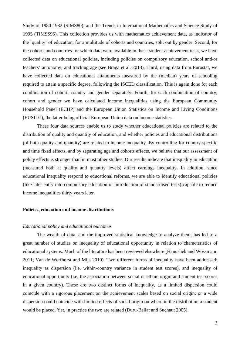
Figure 1 shows the two forms of inequality with regard to mathematics achievement, using

the Trends in International Mathematics and Science Study of 2011 (TIMSS 2011, grade 8) and the

OECD’s Programme for International Student Assessment of 2009 (PISA 2009, 15-year olds).

Inequality as dispersion is measured by the standard deviation in mathematics achievement.

Inequality of opportunity is measured by the effect of the number of books in the household (a

useful indicator of social background, Schütz et al. 2008) on mathematics achievement. Books in

the household are measured as the within-country proportional score, ranging from 0-1, and

mathematics is measured using a factor score on five plausible values. Figure 1 shows a positive

association between the two forms of inequality. Countries with larger dispersions have, on average,

also a stronger relationship between social background and student achievement. At the country

level, the two forms of inequality are correlated at ρ=0.7, in both datasets.

Figure 1: Inequality as dispersion and inequality of opportunities

CANFIN

RUS

JPN

ITASVN

HKG

SWENOR

USA

ISR

CHLNZLAUSGBR

TUR

TWN

HUN

KOR

.6.7

.8.9

11.

1st

anda

rd d

evia

tion

.5 1 1.5 2effect of books in household on math score

r = 0.71, p < 0.01source: TIMSS 2011 (grade 8)

MEX

JPN

LVAFIN

RUS

ISLCANITA

CHL

ISR

HKG

GRCNORKOR

DNKLIENLD

TURAUS

IRL

SVN

PRT

NZL

USA

SWE

POL

SVKCHEESPAUT

GBR

BEL

BGRDEUCZE

HUN

FRA

LUX

.6.7

.8.9

11.

1st

anda

rd d

evia

tion

.5 1 1.5 2effect of books in household on math score

r = 0.66, p < 0.01source: PISA 2009 (15 year olds)

The level of inequality in a school system seems to be related to the educational institutional

structure in a society. Earlier research has focused on several indicators of educational systems,

including early tracking, school accountability, the usage of centralized tests, the existence of

(public) early childhood education, and the size of the private sector.

One of the main factors related to inequality is the extent to which, and at which moment,

students are tracked in different educational trajectories. Early selection in the educational system is

5

known to be associated to higher levels of inequality in student test scores and educational

attainment by social origin (Bol and Van de Werfhorst 2013; Brunello and Checchi 2007; Horn

2009; Husén 1973; Marks 2005; Pfeffer 2008; Schütz et al. 2008). Also ethnic inequalities are

larger in early tracking systems than in comprehensive systems (Cobb-Clark et al. 2012; Entorf and

Lauk 2008, but see Dronkers and De Heus 2010). More strongly differentiated systems are also

associated to more realistic expectations of students concerning future educational attainment

(Buchmann and Dalton 2002; Buchmann and Park 2009; Kerckhoff 1977), which may explain the

relatively early formation of political interests (Koçer and Van de Werfhorst 2012). Importantly,

especially early tracking, and not so much the vocational sector in upper secondary education, is

related to larger inequalities of opportunity (Brunello and Checchi 2007; Bol and Van de Werfhorst

2013). A strong vocational sector in the education system functions rather inclusionary rather than

diverging (cf. Arum and Shavit 1995; Shavit and Müller 2000).

The evidence on the relationship between early differentiation/tracking and inequality as

dispersion is more mixed. Some have reported higher dispersions in countries with more intensified

forms of between-school differentiation/tracking (Hanushek and Wössmann 2005; Huang 2009;

Montt 2011), whereas findings of other studies do not point in that direction (Vandenberge 2006;

Micklewright and Schnepf 2007).

The evidence is also more mixed with regard to the relationship between other

characteristics of educational systems and inequalities. The size of the private schooling sector has

been found to be uncorrelated to the level of inequality by social origin (Pfeffer 2008; Bol and Van

de Werfhorst 2013). School accountability is associated to lower inequalities in student

achievement by parental education (Wössmann 2005). Lower levels of ethnic inequality are found

in systems with an earlier starting age of compulsory education (Cobb-Clark et al. 2012), with

centralized examinations, and a small private schooling sector (Cobb-Clark et al. 2012; Wössmann

2005). Larger private contributions to early childhood education exacerbate income inequalities

between families, which may impact unequal take-up and benefit from it (Meyers and Gornick

2003). But more generally Hanushek and Wössmann (2011) conclude that country characteristics

related to resources have limited effects on student learning, whereas other institutional effects

relating to the structure of schools have stronger impacts.

Educational distributions and income distributions

The relationship between education and earnings has a long tradition in the economic and

sociological literature (see Card 1999 and Heckman et al. 2006 for reviews of the Mincerian

approach). Less attention has been devoted to the relationship between the distribution of

6

educational attainments and the distribution of earnings (see Peracchi 2006, De Gregorio and Lee

2002 and Rodriguez-Pose and Selios 2009 for notable exceptions), possibly because the difficulty

of identifying clear causal links between the two, given the presence of unobservables. An increase

in earnings inequality may prevent educational investments when households are liquidity

constrained (Galor 2012), but may also represent an incentive to acquire further education. General

equilibrium models should account for the relative speeds of expansion of demand and supply for

skills (the so-called “Timbergen race”: see Acemoglu and Autor 2011; Goldin and Katz 2009).

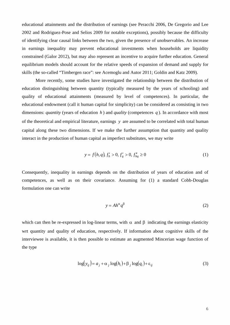
More recently, some studies have investigated the relationship between the distribution of

education distinguishing between quantity (typically measured by the years of schooling) and

quality of educational attainments (measured by level of competences). In particular, the

educational endowment (call it human capital for simplicity) can be considered as consisting in two

dimensions: quantity (years of education h ) and quality (competences q ). In accordance with most

of the theoretical and empirical literature, earnings y are assumed to be correlated with total human

capital along these two dimensions. If we make the further assumption that quantity and quality

interact in the production of human capital as imperfect substitutes, we may write

( ) 0,0,0,, ≥′′>′>′= hqqh fffqhfy (1)

Consequently, inequality in earnings depends on the distribution of years of education and of

competences, as well as on their covariance. Assuming for (1) a standard Cobb-Douglas

formulation one can write

βα= qAhy (2)

which can then be re-expressed in log-linear terms, with α and β indicating the earnings elasticity

wrt quantity and quality of education, respectively. If information about cognitive skills of the

interviewee is available, it is then possible to estimate an augmented Mincerian wage function of

the type

( ) ( ) ( ) ijijijjij qhay ε+β+α+= logloglog (3)

7

where i indicates the individual and j a specific labour market (typically a country/region).

Equation (3) has been estimated by Blau and Kahn (2005) using micro-data from IALS.1 They

claim that the greater dispersion of cognitive test scores in the United States plays a part in

explaining higher U.S. wage inequality. The estimated α̂ and β̂ give us an idea of the relative

contribution of quantity and quality of education in generating income inequality.2 In the same vein,

using the Canadian file of the same survey, Green and Riddell (2003) estimate a linear polynomial

version of equation (3), showing that the impact of literacy on earnings does not vary across

quantiles of the earnings distribution, while the interaction of schooling and literacy is statistically

insignificant. This result can be interpreted as a signal that competences provide an autonomous

contribution to observed inequality, conditional on identical school attainment. Freeman and

Schettkat (2001) follow a parallel approach when comparing US and Germany earnings inequality,

by comparing the distribution of earnings at different points of the distribution of competences in

the adult population using the same IALS survey. They show that US is characterised by greater

inequality in competences than Germany, which is reflected into greater inequality in earnings, and

they attribute this difference to both the educational system (the German apprenticeship system

would raise the bottom of the competence distribution) and the bargaining structure (Germany is

characterised by stronger union movement than US). Also a more recent study has found a cross-

sectional correlation between a country’s level of inequality in adult skills (using PIAAC 2012 data)

and income inequality (Solga 2014).

The main problem of this research strategy is the potential endogeneity of the right-hand

side regressors, since more talented individuals may possess higher level of competences (as well as

achieve higher educational attainments) while obtaining higher earnings. In the absence of credible

instruments, it is hard to accept a causal interpretation of previous results. In addition, competences

are typically measured at the very same time when information on earnings is collected (cf. Solga

2014). But competences are (positively) correlated with educational attainment as well as with

labour market participation, thus requiring an appropriate modelling of the self-selection into the

labour market.

Ideally, one would require a dataset where competences were predetermined with respect to

schooling, which in turn were predetermined with respect to the transition to the labour market.

1 IALS is a survey collecting information on adult literacy in representative samples for some OECD countries, implemented in different years - 1994, 1996, 1998 - for different countries using a common questionnaire. The central element of the survey was the direct assessment of the literacy skills of respondents, but the background questionnaire also included detailed information on individual socio-demographic characteristics. In the public use version of the file, earnings were made available in categorical form, but the authors got access to the actual value. For more information, see http://www.statcan.gc.ca/dli-ild/data-donnees/ftp/ials-eiaa-eng.htm) 2 They write “For example, a one standard deviation increase in test scores raises wages by 5.3 to 15.9 percent for men and 0.7 to 16.2 percent for women [our β coefficient], while a one standard deviation increase in education raises wages by 4.8 to 16.8 percent for men and 6.8 to 26.6 percent for women. [our α coefficient].”

8

Unfortunately, these dataset do exist in a few countries where longitudinal datasets were started

several decades ago (US, UK, Sweden), but they hardly usable in a cross-country perspective. This

has led us to pursue an alternative strategy of country/cohort analysis, matching aggregate

inequality measures of competences, schooling and earnings based on the birth year of the relevant

cohort. Bedard and Ferrall (2003), who study the correlation between the distribution of

competences and the wage distribution of workers in the same birth cohorts, have already followed

a similar strategy. They show that Lorenz curves for a cohort’s wages always lay above the cohort’s

test score Lorenz curve. However, in their analysis, they do not take into account the mediating role

played by educational attainment. Nor did they investigate the relevance of education policies,

which, as we demonstrate, are highly influential on the distribution of education and incomes.

In the present paper we amend for this weakness by explicitly including inequality measures

for schooling, and taking into account the potential endogeneity of these different dimensions of

human capital. We also significantly extend the sample size, by considering repeated observations

of the same cohort over different points of their life cycles. This strategy has pros and cons. The

pros are represented by the possibility of potentially identifying causal effects of the human capital

distribution onto the earnings distribution. The cons are working with aggregate data, which

introduce possible confounding factors, which are only partially cured by including country/year

fixed effects. In addition, aggregate data dramatically reduces the degrees of freedom, incurring in

small sample problems when estimating. Overall, we deem that advantages overwhelm

disadvantages, and that the present exercise may contribute to the advancement of our knowledge.

Empirical strategy

Let us start with a linearised version of equation (3), which reads as

 

ijijijijjij qhay ε+′+β+α+= Xγ (4)

The inequality observed in the distribution of y will depend on the inequality in both quality q and

quantity h of education, as well as on the distribution of any other observables in the vector iX

(like age, gender, ethnicity and so on) or unobservable component ε . Given the non-zero

correlation between education and unobservables, it is generally impossible to decompose observed

earnings inequality into separated contributions of underlying factors in a consistent way.3 The use

3 As an illustrative example consider for example the inequality measure provided by the Gini concentration index. Neglect for simplicity the differences in observables described by iX in equation (4), rewrite it as

9

of decomposable inequality indices (like Theil) does not solve our problem, since they allow for

between/within group decomposition without separating covarying variables (like quantity and

quality of education).

Given the practical impossibility of modelling the structural relationship between the

underlying distributions, we have resorted to the more modest strategy of studying the correlation

among inequality measures, from which we can still deduce educational policy relevant

propositions. By indicating with ( )xI a generic inequality indicator, we posit that an equivalent of

equation (4) can be expressed as

( ) ( ) ( ) jj qIhIyI ω+β+α+δ= (5)

where jδ is a country/year fixed effect capturing any other sort of earnings inequality variation,

while α and β measure the correlation between (the distribution of) various dimensions of human

capital (quantity and quality) and earnings (or income) inequality. If h and/or q are measured well

in advance with respect to y (in our case h is measured at the end of schooling by the maximal

educational attainment, q is measured at the age of 14, while y is measured alternatively at the

ages of 28, 44 and 59), one is tempted to provide a causal interpretation of statements like “a

reduction in inequality in test scores is associated to a β -reduction in income inequality”. However,

unobservable components at country level (like competitiveness, solidarity, ethnic fractionalisation

and so on) may drive both dimension of inequality, leading to biased estimates of the relevant

coefficients. Accounting for this possibility, we have resorted to an instrumental variable strategy to

estimate equation (5) leading to

( )( )( ) ( ) ( )⎪

⎪⎩

⎪⎪⎨

⎧

ω+β+α+δ=

+′+=

+′+=

jj

jjjj

jjjj

qIhIyI

gcqI

eahI

ˆˆZd

Zb

(6)

ijijijjij qhay ε+β+α+= . The Gini index for a generic country/region j can be computed according to

( ) ( ) ( ) ( )∑∑∑∑ ε−ε+−β+−αμ

=−μ

=i k

kikikiyi k

kiy

qqhhyyyGini2

12

1 . If one is available to accept that: i) the rank

correlation between quality and quantity is one (namely students with the highest level of competences also obtain the highest educational attainments – in symbols kiki qqiffhh >> ); ii) the unexpected component in earnings is small relative to the predictable component (in symbols iqha iii ∀ε>β+α+ , ), then it is possible to express the earnings

inequality as ( ) ( ) residualqGinihGiniyGiniy

q

y

h +μ

μβ+

μμ

α=)( . Thus only under implausible assumptions one can infer

the inequality contribution of different component from the estimation of structural parameters in equation like (4).

10

where the educational inequality measures in equation (5) are replaced by their projections obtained

from a vector of (supposedly) exogenous variables pertaining reforms in the educational sectors

affecting the relevant birth cohorts. We thus exploit both geographical and temporal variations in

educational reforms by government to obtain unbiased estimates of the causal impact of educational

inequality onto income inequality.

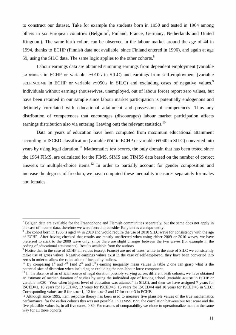
We have already suggested that an ideal dataset should measure quantity and quality of

education at the age of exiting the educational system and earnings at a later age, following the

entrance in the labour market. At the best of our knowledge, such a dataset does not exist with

sufficient country coverage. For this reason, we have created a new dataset by combining data on

measured inequality from students’ tests with data on measured inequality on earnings of the same

birth cohorts, gender and country.

Data on students’ competences are obtained from three early surveys on mathematical

competences of 14-year-old students conducted in past decades (FIMS 1964 was the first

international survey testing mathematical competences of students born in or around 1950; SIMS

1980-82 tested students born in or around 1966 and TIMSS 1995 tested students born in or around

1981)4. We thus start with a population composed by three birth cohorts, born in 1950, 1966 and

1981 respectively, in countries that participated to the earliest students surveys. Data on schooling

and labour market outcomes for the same cohorts can be obtained from representative samples of

the corresponding population at later stages. However, if observed at the same point in time, we

would be confusing cohorts and age effects (namely, older cohorts are characterised by higher level

of competences and earnings inequalities). For this reason, we have resorted to two available

datasets existing at European level and reporting data on earnings and incomes. The first one is the

European Community Household Panel (ECHP), which started in 1994.5 The second is the

European Union Statistics on Income and Living Conditions (EUSILC), which started in 2004 and

is updated annually.6 We selected the 1994 ECHP wave because it was the earliest available, while

we resorted to the 2009 SILC wave because it was the first survey reporting consistent information

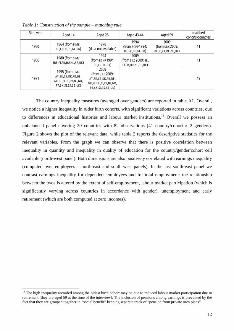
on gross incomes for all participating countries. In table 1 we show the matching rule we followed 4 The FIMS (First International Mathematics Study) was conducted in 1964 to investigate the outcomes of school systems in cross-country perspective and repeated in 1980 when the SIMS (Second International Mathematics Study) took place. The third round was carried out in 1995 when the TIMSS (Trends in International Mathematics and Science Study) was administered. The data are accessible through the International Association for the Evaluation of Educational Achievement, IEA, at www.iea.nl. 5 ECHP (European Community Household Panel) is a panel survey in which a sample of households and persons has been interviewed year after year, from 1994 to 2001 (8 waves), for the 14 European countries that were members of the EU in 1994. For more information see http://epp.eurostat.ec.europa.eu/portal/page/portal/microdata/echp. 6 EUSILC (European Union Statistics on Income and Living Conditions) is a collection of comparable multidimensional microdata covering EU countries plus Iceland and Norway. EUSILC is a project developed by EUROSTAT, run yearly since 2004 and including both cross-section and longitudinal surveys. For more information, see http://epp.eurostat.ec.europa.eu/portal/page/portal/microdata/eu_silc

11

to construct our dataset. Take for example the students born in 1950 and tested in 1964 among

others in six European countries (Belgium7, Finland, France, Germany, Netherlands and United

Kingdom). The same birth cohort can be observed in the labour market around the age of 44 in

1994, thanks to ECHP (Finnish data not available, since Finland entered in 1996), and again at age

59, using the SILC data. The same logic applies to the other cohorts.8

Labour earnings data are obtained summing earnings from dependent employment (variable

EARNINGS in ECHP or variable PY010G in SILC) and earnings from self-employment (variable

SELFINCOME in ECHP or variable PY050G in SILC) and excluding cases of negative values.9

Individuals without earnings (housewives, unemployed, out of labour force) report zero values, but

have been retained in our sample since labour market participation is potentially endogenous and

definitely correlated with educational attainment and possession of competences. Thus any

distribution of competences that encourages (discourages) labour market participation affects

earnings distribution also via entering (leaving out) the relevant statistics.10

Data on years of education have been computed from maximum educational attainment

according to ISCED classification (variable EDU in ECHP or variable PE040 in SILC) converted into

years by using legal duration.11 Mathematics test scores, the only domain that has been tested since

the 1964 FIMS, are calculated for the FIMS, SIMS and TIMSS data based on the number of correct

answers to multiple-choice items.12 In order to partially account for gender composition and

increase the degrees of freedom, we have computed these inequality measures separately for males

and females.

7 Belgian data are available for the Francophone and Flemish communities separately, but the same does not apply in the case of income data, therefore we were forced to consider Belgium as a unique entity. 8 The cohort born in 1966 is aged 44 in 2010 and would require the use of 2010 SILC wave for consistency with the age of ECHP. After having checked that results are mostly unaffected when using either 2009 or 2010 waves, we have preferred to stick to the 2009 wave only, since there are slight changes between the two waves (for example in the coding of educational attainments). Results available from the authors. 9 Notice that in the case of ECHP all values (except France) are net of taxes, while in the case of SILC we consistently make use of gross values. Negative earnings values exist in the case of self-employed, they have been converted into zeros in order to allow the calculation of inequality indices. 10 By comparing 1st and 4th (and 2nd and 5th) earning inequality mean values in table 2 one can grasp what is the potential size of distortion when including or excluding the non-labour force component. 11 In the absence of an official source of legal duration possibly varying across different birth cohorts, we have obtained an estimate of median duration of studies by using the individual age of leaving school (variable AGEDU in ECHP or variable PE030 “Year when highest level of education was attained” in SILC), and then we have assigned 7 years for ISCED=1, 10 years for ISCED=2, 13 years for ISCED=3, 15 years for ISCED=4 and 18 years for ISCED=5 in SILC. Corresponding values are 8 for EDU=1, 12 for EDU=2 and 17 for EDU=3 in ECHP. 12 Although since 1995, item response theory has been used to measure five plausible values of the true mathematics performance, for the earlier cohorts this was not possible. In TIMSS 1995 the correlation between our test score and the five plausible values is, in all five cases, 0.89. For reasons of comparability we chose to operationalize math in the same way for all three cohorts.

12

Table 1: Construction of the sample – matching rule Birth year Aged 14 Aged 28 Aged 43-44 Aged 59 matched

cohorts/countries

1950 1964 (from FIMS: BE,FI,FR,DE,NL,UK)

1978 (data not available)

1994 (from ECHP1994: BE,FR,DE,NL,UK)

2009 (from SILC2009:

BE,FI,FR,DE,NL,UK) 11

1966 1980 (from SIMS: (BE,FI,FR,HU,NL,SE,UK)

1994 (from ECHP1994:

BE,FR,NL,UK)

2009 (from SILC2009: BE, FI,FR,HU,NL,SE,UK)

11

1981 1995 (from TIMS:

AT,BE,CZ,DK,FR,DE, GR,HU,IE,IT,LV,NL,NO,

PT,SK,SI,ES,SE,UK)

2009 (from SILC2009:

AT,BE,CZ,DK,FR,DE, GR,HU,IE,IT,LV,NL,NO,

PT,SK,SI,ES,SE,UK)

19

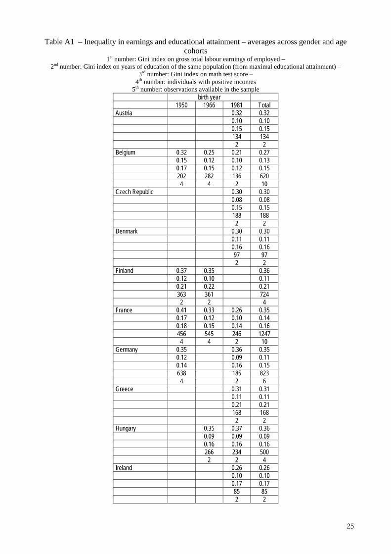
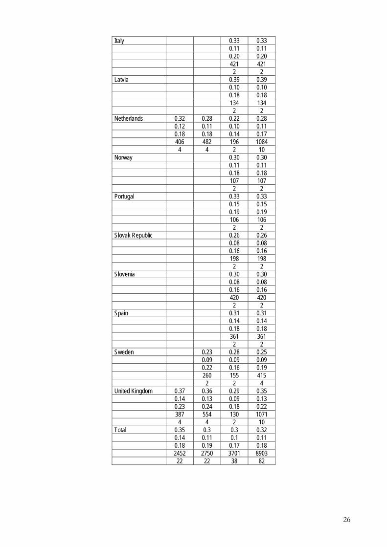
The country inequality measures (averaged over genders) are reported in table A1. Overall,

we notice a higher inequality in older birth cohorts, with significant variations across countries, due

to differences in educational histories and labour market institutions.13 Overall we possess an

unbalanced panel covering 20 countries with 82 observations (41 country/cohort × 2 genders).

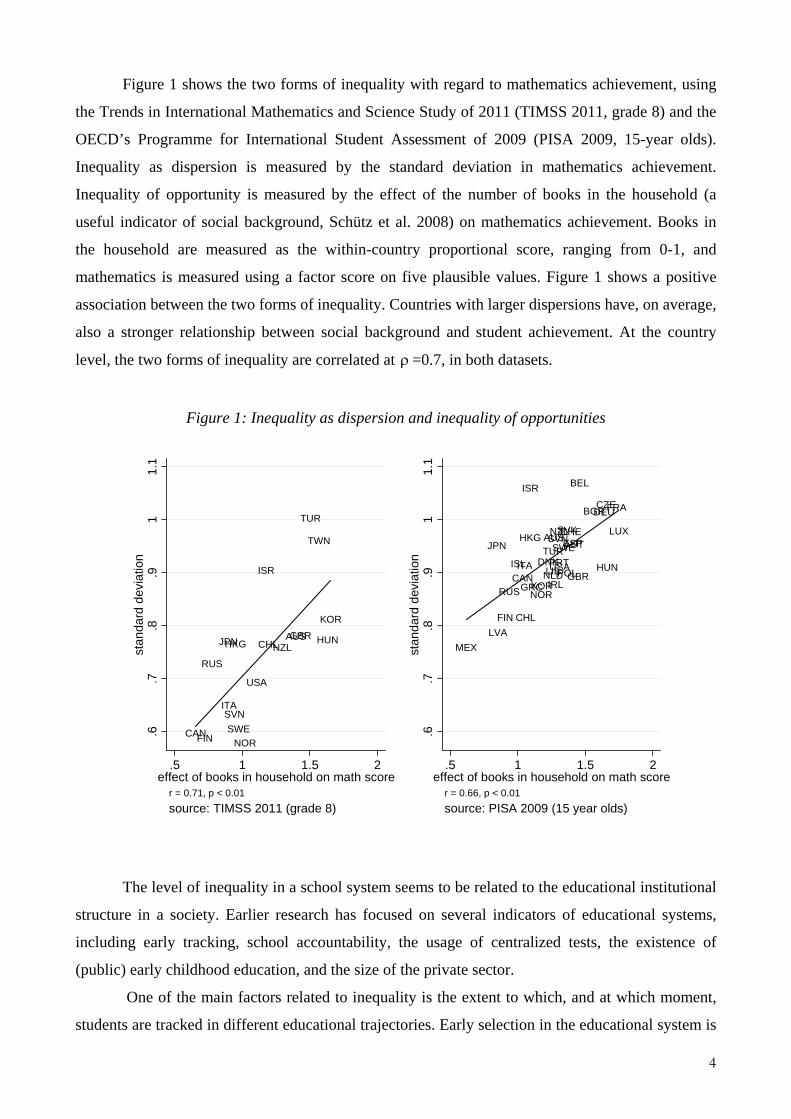
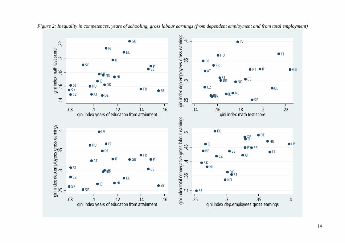
Figure 2 shows the plot of the relevant data, while table 2 reports the descriptive statistics for the

relevant variables. From the graph we can observe that there is positive correlation between

inequality in quantity and inequality in quality of education for the country/gender/cohort cell

available (north-west panel). Both dimensions are also positively correlated with earnings inequality

(computed over employees – north-east and south-west panels). In the last south-east panel we

contrast earnings inequality for dependent employees and for total employment: the relationship

between the twos is altered by the extent of self-employment, labour market participation (which is

significantly varying across countries in accordance with gender), unemployment and early

retirement (which are both computed at zero incomes).

13 The high inequality recorded among the oldest birth cohort may be due to reduced labour market participation due to retirement (they are aged 59 at the time of the interview). The inclusion of pensions among earnings is prevented by the fact that they are grouped together in “social benefit” keeping separate track of “pension from private own plans”.

13

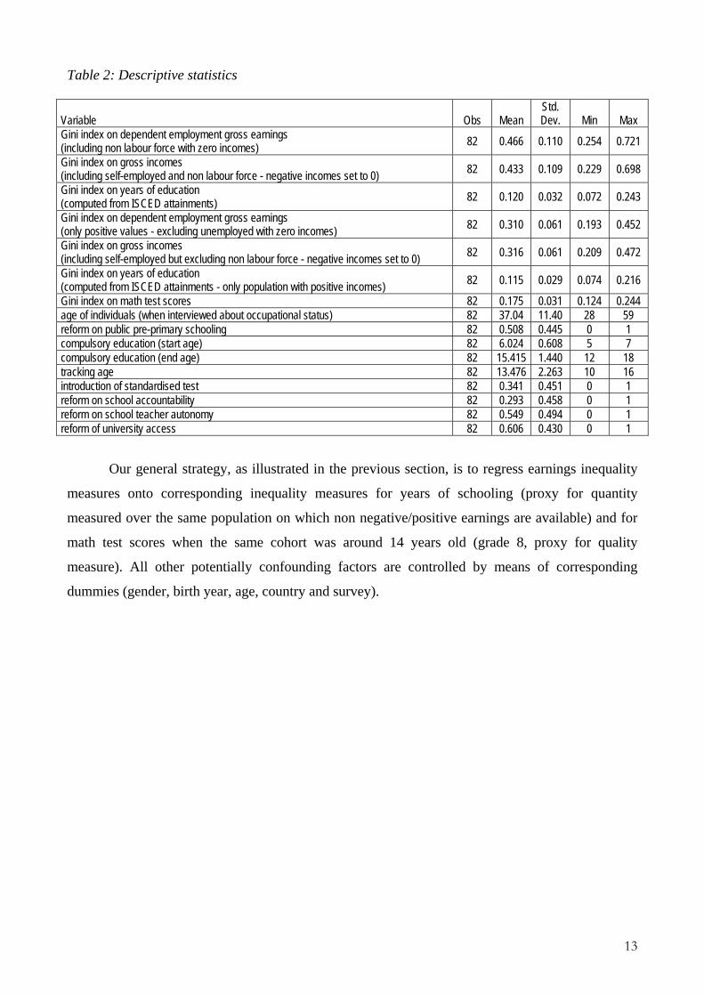
Table 2: Descriptive statistics

Variable Obs Mean Std. Dev. Min Max

Gini index on dependent employment gross earnings (including non labour force with zero incomes) 82 0.466 0.110 0.254 0.721

Gini index on gross incomes (including self-employed and non labour force - negative incomes set to 0) 82 0.433 0.109 0.229 0.698

Gini index on years of education (computed from ISCED attainments) 82 0.120 0.032 0.072 0.243

Gini index on dependent employment gross earnings (only positive values - excluding unemployed with zero incomes) 82 0.310 0.061 0.193 0.452

Gini index on gross incomes (including self-employed but excluding non labour force - negative incomes set to 0) 82 0.316 0.061 0.209 0.472

Gini index on years of education (computed from ISCED attainments - only population with positive incomes) 82 0.115 0.029 0.074 0.216

Gini index on math test scores 82 0.175 0.031 0.124 0.244 age of individuals (when interviewed about occupational status) 82 37.04 11.40 28 59 reform on public pre-primary schooling 82 0.508 0.445 0 1 compulsory education (start age) 82 6.024 0.608 5 7 compulsory education (end age) 82 15.415 1.440 12 18 tracking age 82 13.476 2.263 10 16 introduction of standardised test 82 0.341 0.451 0 1 reform on school accountability 82 0.293 0.458 0 1 reform on school teacher autonomy 82 0.549 0.494 0 1 reform of university access 82 0.606 0.430 0 1

Our general strategy, as illustrated in the previous section, is to regress earnings inequality

measures onto corresponding inequality measures for years of schooling (proxy for quantity

measured over the same population on which non negative/positive earnings are available) and for

math test scores when the same cohort was around 14 years old (grade 8, proxy for quality

measure). All other potentially confounding factors are controlled by means of corresponding

dummies (gender, birth year, age, country and survey).

14

Figure 2: Inequality in competences, years of schooling, gross labour earnings (from dependent employment and from total employment)

ATBE

CZ DE

DK

EL

ES

FI

FR

GB

HUIE

IT

LVNLNO

PTSE

SISK

.14.16

.18.2

.22gin

i inde

x math

test

scor

e

.08 .1 .12 .14 .16gini index years of education from attainment

AT

BE

CZ

DE

DK

EL

ES

FI

FRGB

HU

IE

IT

LV

NL

NO

PT

SE

SI

SK

.25.3

.35.4

gini in

dex d

ep.em

ploye

es gr

oss e

arnin

gs

.14 .16 .18 .2 .22gini index math test score

AT

BE

CZ

DE

DK

EL

ES

FI

FRGB

HU

IE

IT

LV

NL

NO

PT

SE

SI

SK

.25.3

.35.4

gini in

dex d

ep.em

ploye

es gr

oss e

arnin

gs

.08 .1 .12 .14 .16gini index years of education from attainment

ATBE

CZ

DE

DK

EL

ES FIFR

GBHUIE

ITLV

NL

NO

PT

SE

SI

SK

.3.35

.4.45

.5gin

i inde

x tota

l non

nega

tive g

ross

labo

ur ea

rning

s

.25 .3 .35 .4gini index dep.employees gross earnings

15

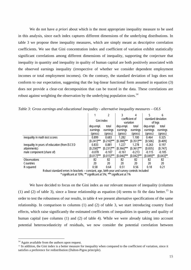
We do not have a priori about which is the most appropriate inequality measure to be used

in this analysis, since each index captures different dimensions of the underlying distributions. In

table 3 we propose three inequality measures, which are simply meant as descriptive correlation

coefficients. We see that Gini concentration index and coefficient of variation exhibit statistically

significant correlations among different dimensions of inequality, supporting the conjecture that

inequality in quantity and inequality in quality of human capital are both positively associated with

the observed earnings inequality (irrespective of whether we consider dependent employment

incomes or total employment incomes). On the contrary, the standard deviation of logs does not

conform to our expectation, suggesting that the log-linear functional form assumed in equation (3)

does not provide a clear-cut decomposition that can be traced in the data. These correlations are

robust against weighting the observation by the underlying population sizes.14

Table 3: Gross earnings and educational inequality - alternative inequality measures – OLS 1 2 3 4 5 6

Gini index coefficient of variation

standard deviation of logs

dep.empl. earnings (gross)

total earnings (gross)

dep.empl. earnings (gross)

total earnings (gross)

dep.empl. earnings (gross)

total earnings (gross)

inequality in math test scores 0.899 0.683 1.282 1.100 0.464 0.325 [0.241]*** [0.210]*** [0.388]*** [0.351]*** [0.506] [0.409]

0.833 0.881 1.227 1.278 -0.263 0.197 inequality in years of education (from ISCED attainments) [0.258]*** [0.231]*** [0.366]*** [0.361]*** [0.835] [0.747] male component (share of) -0.078 -0.107 -0.161 -0.213 -0.115 -0.105 [0.017]*** [0.015]*** [0.046]*** [0.042]*** [0.049]** [0.043]** Observations 82 82 82 82 82 82 Countries 20 20 20 20 20 20 R-squared 0.58 0.64 0.51 0.56 0.18 0.21

Robust standard errors in brackets – constant, age, birth year and survey controls included * significant at 10%; ** significant at 5%; *** significant at 1%

We have decided to focus on the Gini index as our relevant measure of inequality (columns

(1) and (2) of table 3), since a linear relationship as equation (4) seems to fit the data better.15 In

order to test the robustness of our results, in table 4 we present alternative specifications of the same

relationship. In comparison to columns (1) and (2) of table 3, we start introducing country fixed

effects, which raise significantly the estimated coefficients of inequalities in quantity and quality of

human capital (see columns (1) and (2) of table 4). While we were already taking into account

potential heteroscedasticity of residuals, we now consider the potential correlation between

14 Again available from the authors upon request. 15 In addition, the Gini index is a better measure for inequality when compared to the coefficient of variation, since it satisfies a preference for redistribution (Dalton-Pigou principle).

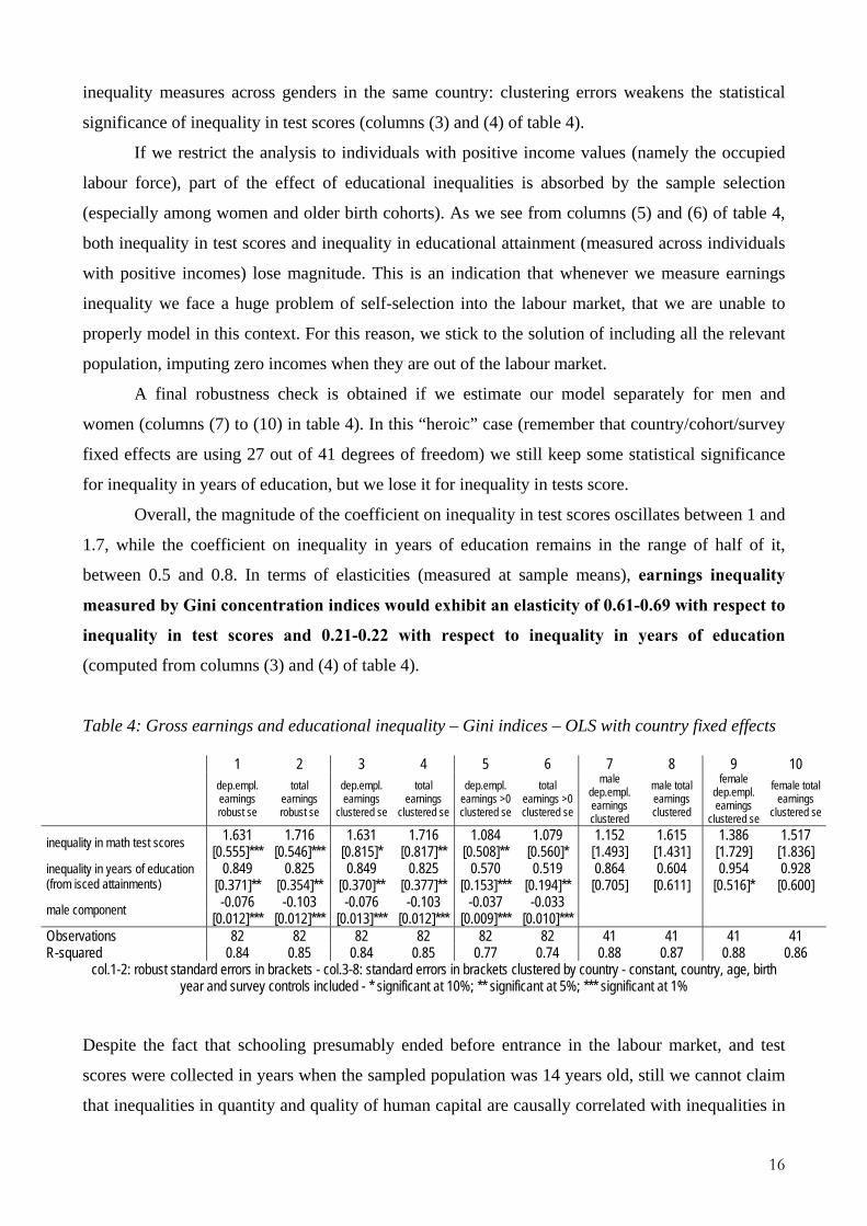
16

inequality measures across genders in the same country: clustering errors weakens the statistical

significance of inequality in test scores (columns (3) and (4) of table 4).

If we restrict the analysis to individuals with positive income values (namely the occupied

labour force), part of the effect of educational inequalities is absorbed by the sample selection

(especially among women and older birth cohorts). As we see from columns (5) and (6) of table 4,

both inequality in test scores and inequality in educational attainment (measured across individuals

with positive incomes) lose magnitude. This is an indication that whenever we measure earnings

inequality we face a huge problem of self-selection into the labour market, that we are unable to

properly model in this context. For this reason, we stick to the solution of including all the relevant

population, imputing zero incomes when they are out of the labour market.

A final robustness check is obtained if we estimate our model separately for men and

women (columns (7) to (10) in table 4). In this “heroic” case (remember that country/cohort/survey

fixed effects are using 27 out of 41 degrees of freedom) we still keep some statistical significance

for inequality in years of education, but we lose it for inequality in tests score.

Overall, the magnitude of the coefficient on inequality in test scores oscillates between 1 and

1.7, while the coefficient on inequality in years of education remains in the range of half of it,

between 0.5 and 0.8. In terms of elasticities (measured at sample means), earnings inequality

measured by Gini concentration indices would exhibit an elasticity of 0.61-0.69 with respect to

inequality in test scores and 0.21-0.22 with respect to inequality in years of education

(computed from columns (3) and (4) of table 4).

Table 4: Gross earnings and educational inequality – Gini indices – OLS with country fixed effects

1 2 3 4 5 6 7 8 9 10

dep.empl. earnings robust se

total earnings robust se

dep.empl. earnings

clustered se

total earnings

clustered se

dep.empl. earnings >0 clustered se

total earnings >0 clustered se

male dep.empl. earnings clustered

male total earnings clustered

female dep.empl. earnings

clustered se

female total earnings

clustered se

1.631 1.716 1.631 1.716 1.084 1.079 1.152 1.615 1.386 1.517 inequality in math test scores [0.555]*** [0.546]*** [0.815]* [0.817]** [0.508]** [0.560]* [1.493] [1.431] [1.729] [1.836] 0.849 0.825 0.849 0.825 0.570 0.519 0.864 0.604 0.954 0.928 inequality in years of education

(from isced attainments) [0.371]** [0.354]** [0.370]** [0.377]** [0.153]*** [0.194]** [0.705] [0.611] [0.516]* [0.600] -0.076 -0.103 -0.076 -0.103 -0.037 -0.033 male component [0.012]*** [0.012]*** [0.013]*** [0.012]*** [0.009]*** [0.010]***

Observations 82 82 82 82 82 82 41 41 41 41 R-squared 0.84 0.85 0.84 0.85 0.77 0.74 0.88 0.87 0.88 0.86

col.1-2: robust standard errors in brackets - col.3-8: standard errors in brackets clustered by country - constant, country, age, birth year and survey controls included - * significant at 10%; ** significant at 5%; *** significant at 1%

Despite the fact that schooling presumably ended before entrance in the labour market, and test

scores were collected in years when the sampled population was 14 years old, still we cannot claim

that inequalities in quantity and quality of human capital are causally correlated with inequalities in

17

earnings and incomes. In order to strengthen the claim of causality, in table 5 we resort to

instrumental variable estimation, which has the additional advantage of allowing the study of the

impact of educational reforms on income inequality via their impact on inequality in quantity and

quality of human capital. As measures of institutional design we exploit here the measures of

educational reforms constructed by Braga et al. (2013) covering various stages of schooling.16

For ease of comparison in columns (1) and (2) of table 5 we have reproduced columns (3)

and (4) of previous table 4. In columns (3) and (4) we present the corresponding IV estimations

using a 2SLS estimator, while in columns (5) and (6) a GMM estimator is proposed. The bottom

part of the table reports the first stage coefficients of the regression of the potentially endogenous

variables (inequality in quantity and inequality in quality of education) onto the instruments

represented by measured reforms. Starting with first stage coefficients signs and significance, we

notice that inequality in years of education is reduced in countries that expanded pre-primary

education or postponed the beginning age for compulsory education, while the school leaving age

seems to have a counterintuitive positive correlation.17 Postponing the age at which students have to

choose the secondary school track (wherever the educational system is stratified, like in Austria,

Germany, Italy and the Netherlands) seem to increase both inequalities in schooling and test

scores.18 On the contrary, strengthening the standardisation of national educational systems through

the introduction of student testing is associated to a reduction of inequality. Finally, consistently

with the results of Braga et al. (2013), increasing schools/teachers and universities autonomy

reinforce their potential competitiveness, at the expenses of increased educational inequality.

Similar patterns are observed in the case of competence inequality. The statistical significance of

these effects relies on the method utilised to estimate the variance-covariance matrix: while

educational reforms remain significant for test score inequality under both IV estimators, they tend

to lose significance in the case of schooling inequality when passing to GMM method of estimation.

Notice that all regressions control for country, birth year, age and survey fixed effects, so that

reform impacts are identified by time variation within the countries and/or gender differential

impacts within each country/year. Using the predicted inequalities in quantity and quality of human

capital as regressors for income inequality, we observe that their coefficients lose statistical 16 Braga et al (2013) claim that educational reforms may be effective in reducing inequality in schooling (where this is measured by the Atkinson index computed over years of education), while Bol and Van de Werfhorst (2013) have constructed measure of stratification of the secondary school systems (differentiation of students in different tracks, provision of vocationally specific skills and nationwide standardization of the educational system) showing in a cross-sectional framework that the institutional design may be effective in shaping the distribution of student competences. 17 Brunello et al. (2009) find that the expansion of duration of compulsory education (which in the present framework corresponds to the difference between entry and exit ages) reduces income inequality. According to the results of table 5 the opposite situation occurs, since expansion of compulsory education may be produced by either lowering the starting age or raising the leaving age, in both case yielding a positive impact on inequality in years of education. 18 This latter effect contradicts standard findings in the literature on determinants of test scores(see for example Hanusheck and Woessman 2005) while it is consistent with the findings for inequality in years of education (Brunello and Checchi 2007)

18

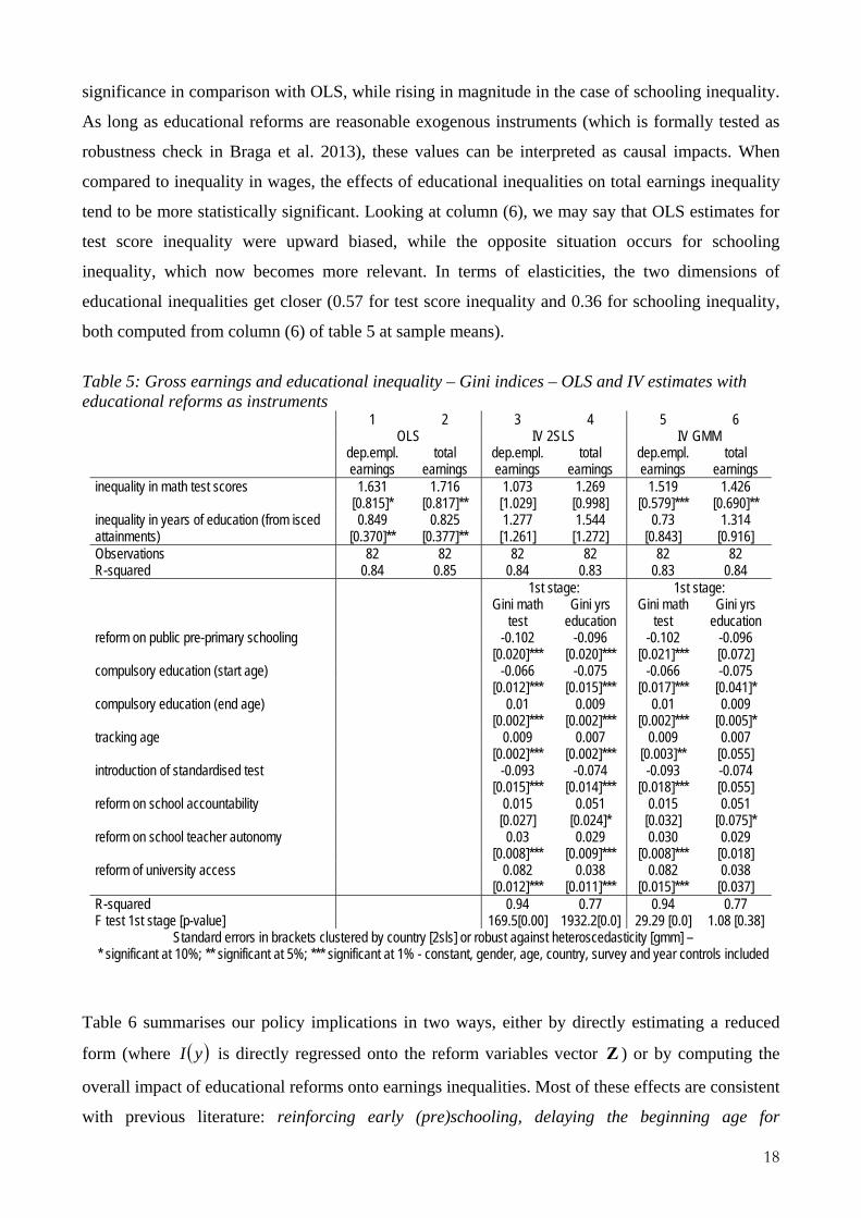
significance in comparison with OLS, while rising in magnitude in the case of schooling inequality.

As long as educational reforms are reasonable exogenous instruments (which is formally tested as

robustness check in Braga et al. 2013), these values can be interpreted as causal impacts. When

compared to inequality in wages, the effects of educational inequalities on total earnings inequality

tend to be more statistically significant. Looking at column (6), we may say that OLS estimates for

test score inequality were upward biased, while the opposite situation occurs for schooling

inequality, which now becomes more relevant. In terms of elasticities, the two dimensions of

educational inequalities get closer (0.57 for test score inequality and 0.36 for schooling inequality,

both computed from column (6) of table 5 at sample means).

Table 5: Gross earnings and educational inequality – Gini indices – OLS and IV estimates with educational reforms as instruments

1 2 3 4 5 6 OLS IV 2SLS IV GMM

dep.empl. earnings

total earnings

dep.empl. earnings

total earnings

dep.empl. earnings

total earnings

1.631 1.716 1.073 1.269 1.519 1.426 inequality in math test scores [0.815]* [0.817]** [1.029] [0.998] [0.579]*** [0.690]** 0.849 0.825 1.277 1.544 0.73 1.314 inequality in years of education (from isced

attainments) [0.370]** [0.377]** [1.261] [1.272] [0.843] [0.916] Observations 82 82 82 82 82 82 R-squared 0.84 0.85 0.84 0.83 0.83 0.84 1st stage: 1st stage:

Gini math

test Gini yrs

education Gini math

test Gini yrs

education -0.102 -0.096 -0.102 -0.096 reform on public pre-primary schooling [0.020]*** [0.020]*** [0.021]*** [0.072] -0.066 -0.075 -0.066 -0.075 compulsory education (start age) [0.012]*** [0.015]*** [0.017]*** [0.041]* 0.01 0.009 0.01 0.009 compulsory education (end age) [0.002]*** [0.002]*** [0.002]*** [0.005]* 0.009 0.007 0.009 0.007 tracking age [0.002]*** [0.002]*** [0.003]** [0.055] -0.093 -0.074 -0.093 -0.074 introduction of standardised test [0.015]*** [0.014]*** [0.018]*** [0.055] 0.015 0.051 0.015 0.051 reform on school accountability [0.027] [0.024]* [0.032] [0.075]* 0.03 0.029 0.030 0.029 reform on school teacher autonomy [0.008]*** [0.009]*** [0.008]*** [0.018] 0.082 0.038 0.082 0.038 reform of university access [0.012]*** [0.011]*** [0.015]*** [0.037]

R-squared 0.94 0.77 0.94 0.77 F test 1st stage [p-value] 169.5[0.00] 1932.2[0.0] 29.29 [0.0] 1.08 [0.38]

Standard errors in brackets clustered by country [2sls] or robust against heteroscedasticity [gmm] – * significant at 10%; ** significant at 5%; *** significant at 1% - constant, gender, age, country, survey and year controls included

Table 6 summarises our policy implications in two ways, either by directly estimating a reduced

form (where ( )yI is directly regressed onto the reform variables vector Z ) or by computing the

overall impact of educational reforms onto earnings inequalities. Most of these effects are consistent

with previous literature: reinforcing early (pre)schooling, delaying the beginning age for

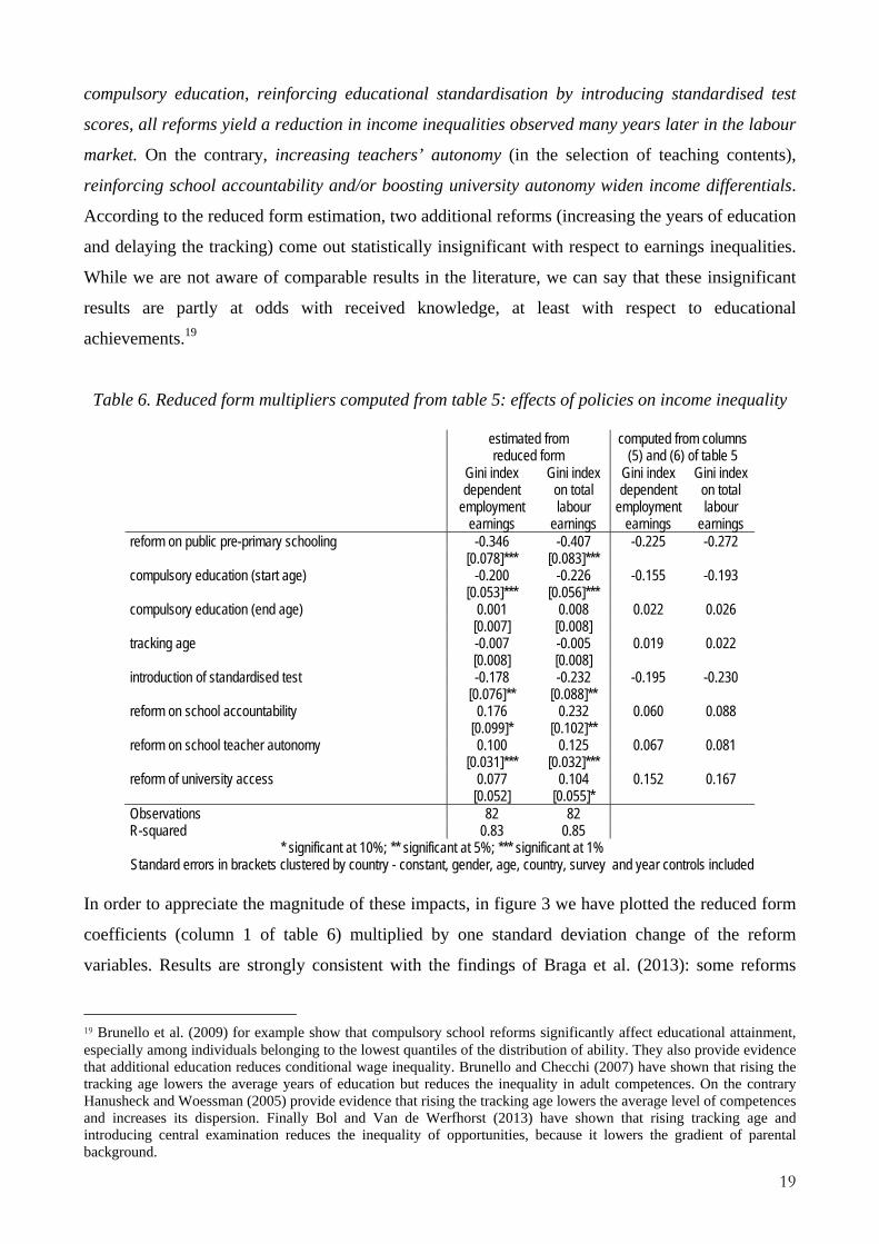
19

compulsory education, reinforcing educational standardisation by introducing standardised test

scores, all reforms yield a reduction in income inequalities observed many years later in the labour

market. On the contrary, increasing teachers’ autonomy (in the selection of teaching contents),

reinforcing school accountability and/or boosting university autonomy widen income differentials.

According to the reduced form estimation, two additional reforms (increasing the years of education

and delaying the tracking) come out statistically insignificant with respect to earnings inequalities.

While we are not aware of comparable results in the literature, we can say that these insignificant

results are partly at odds with received knowledge, at least with respect to educational

achievements.19

Table 6. Reduced form multipliers computed from table 5: effects of policies on income inequality

estimated from reduced form

computed from columns (5) and (6) of table 5

Gini index dependent

employment earnings

Gini index on total labour

earnings

Gini index dependent

employment earnings

Gini index on total labour

earnings -0.346 -0.407 -0.225 -0.272 reform on public pre-primary schooling

[0.078]*** [0.083]*** -0.200 -0.226 -0.155 -0.193 compulsory education (start age)

[0.053]*** [0.056]*** 0.001 0.008 0.022 0.026 compulsory education (end age) [0.007] [0.008] -0.007 -0.005 0.019 0.022 tracking age [0.008] [0.008] -0.178 -0.232 -0.195 -0.230 introduction of standardised test

[0.076]** [0.088]** 0.176 0.232 0.060 0.088 reform on school accountability

[0.099]* [0.102]** 0.100 0.125 0.067 0.081 reform on school teacher autonomy

[0.031]*** [0.032]*** 0.077 0.104 0.152 0.167 reform of university access [0.052] [0.055]*

Observations 82 82 R-squared 0.83 0.85

* significant at 10%; ** significant at 5%; *** significant at 1% Standard errors in brackets clustered by country - constant, gender, age, country, survey and year controls included

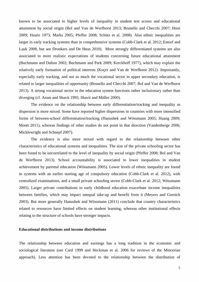
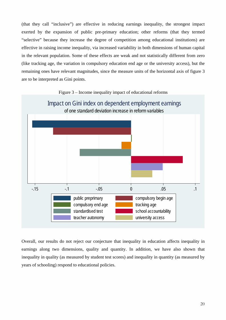
In order to appreciate the magnitude of these impacts, in figure 3 we have plotted the reduced form

coefficients (column 1 of table 6) multiplied by one standard deviation change of the reform

variables. Results are strongly consistent with the findings of Braga et al. (2013): some reforms

19 Brunello et al. (2009) for example show that compulsory school reforms significantly affect educational attainment, especially among individuals belonging to the lowest quantiles of the distribution of ability. They also provide evidence that additional education reduces conditional wage inequality. Brunello and Checchi (2007) have shown that rising the tracking age lowers the average years of education but reduces the inequality in adult competences. On the contrary Hanusheck and Woessman (2005) provide evidence that rising the tracking age lowers the average level of competences and increases its dispersion. Finally Bol and Van de Werfhorst (2013) have shown that rising tracking age and introducing central examination reduces the inequality of opportunities, because it lowers the gradient of parental background.

20

(that they call “inclusive”) are effective in reducing earnings inequality, the strongest impact

exerted by the expansion of public pre-primary education; other reforms (that they termed

“selective” because they increase the degree of competition among educational institutions) are

effective in raising income inequality, via increased variability in both dimensions of human capital

in the relevant population. Some of these effects are weak and not statistically different from zero

(like tracking age, the variation in compulsory education end age or the university access), but the

remaining ones have relevant magnitudes, since the measure units of the horizontal axis of figure 3

are to be interpreted as Gini points.

Figure 3 – Income inequality impact of educational reforms

-.15 -.1 -.05 0 .05 .1

of one standard deviation increase in reform variablesImpact on Gini index on dependent employment earnings

public preprimary compulsory begin agecompulsory end age tracking agestandardised test school accountabilityteacher autonomy university access

Overall, our results do not reject our conjecture that inequality in education affects inequality in

earnings along two dimensions, quality and quantity. In addition, we have also shown that

inequality in quality (as measured by student test scores) and inequality in quantity (as measured by

years of schooling) respond to educational policies.

21

Conclusions and discussion

We studied the relationship between educational policies, educational distributions and income

inequality. Adopting a framework in which educational distributions have both a qualitative and a

quantitative dimension, with quality referring to student performance on standardized tests, and

quantity referring to the attained level of education, we examined whether educational reforms

affect education, and, through education, the distribution of incomes in society. By combining four

different sources of cross-nationally comparative data (international student assessments,

educational attainment, income distributions, and a newly collected data set on educational

reforms), we were able to examine data for cohorts born between 1950 and 1981. Our results

indicated that educational reforms do have an effect on the distribution of the quality and the

quantity of education. The distribution of skills and attainment is furthermore related to the level of

income/earnings inequality in a society. Consequently, educational policies have an impact on the

income and earnings distributions. These findings are supportive of the idea that educational

policies can be part of an effective strategy to address income and earnings distributions.

22

References

Acemoglu, Daron and David Autor. 2011. Skills, Tasks and Technologies: Implications for Employment and Earning. in Orley Ashenfelter and David Card (eds) Handbook of labor economics - vol.4b. Amsterdam: Elsevier North Holland: 1043-1171

Arum, R., and Shavit, Y. (1995). Secondary Vocational Education and the Transition from School to Work. Sociology of Education, 68(July), 187–204.

Bedard, Kelly and Christopher Ferrall. 2003. Wage and test score dispersion: some international evidence. Economics of Education Review 22: 31–43

Blau, Francine and Kahn, Lawrence. 2005. Do cognitive test scores explain higher US wage inequality. Review of Economics and Statistics, 87(1): 184-193.

Bol, Thijs, en Van de Werfhorst, Herman G. (2013). Educational Systems and the Trade-off Between Labor Market Allocation and Equality of Educational Opportunity. Comparative Education Review, 57(2): 285-308.

Braga M., Checchi D. and Meschi E. 2013. Institutional Reforms and Educational Attainment in Europe: A long run perspective. Economic Policy 73: 45-100

Brunello, G., and Checchi, D. (2007). Does school tracking affect equality of opportunity? New international evidence. Economic Policy, 22(52), 781–861.

Brunello, G., Fort, M. and Weber, G. 2009. Changes in Compulsory Schooling, Education and the Distribution of Wages in Europe, Economic Journal, 119(536): 516-539.

Buchmann, C., and Dalton, B. (2002). Interpersonal Influences and Educational Aspirations in 12 Countries: The Importance of Institutional Context. Sociology of Education, 75(2), 99–122.

Buchmann, C., and Park, H. (2009). Stratification and the formation of expectations in highly differentiated educational systems. Research in Social Stratification and Mobility, 27(4), 245–267.

Card, David. 1999. The causal effect of education on earnings. in Ashenfelter, O. and D.Card (eds). Handbook of Labor Economics – vol.3. Amsterdam: Elsevier North Holland: 1801-1863

Cobb-Clark, D. A., Sinning, M., and Stillman, S. (2012). Migrant Youths’ Educational Achievement The Role of Institutions. The ANNALS of the American Academy of Political and Social Science, 643(1), 18–45.

De Gregorio, J. and Lee, J. (2002). Education and Income Inequality: New Evidence From Cross-Country Data. Review of Income and Wealth, 48(3), 395–416.

Dronkers, J., and De Heus, M. (2010). Negative selectivity of Europe’s guest-worker immigration? The educational achievement of children of immigrants compared with native children in their origin countries. In E. De Corte and J. Fenstad (Red.), From Information to Knowledge; from Knowledge to Wisedom: Challenges and Changes facing Higher Education in the Digital Age (pp. 89–104). London: Portland Press. Geraadpleegd van http://mpra.ub.uni-muenchen.de/22213/

Duru-Bellat, Marie and Bruno Suchaut. 2005. L'approche sociologique des effets du contexte scolaire : Méthodes et difficultés. Revue internationale de psychologie sociale 18:5–42.

Entorf, H., and Lauk, M. (2008). Peer effects, social multipliers and migrants at school: an international comparison. Journal of Ethnic and Migration Studies, 34(4), 633–654.

Freeman, Richard and Ronald Schettkat. 2001. Skill Compression, Wage Differentials and Employment: Germany vs. the US. Oxford Economic Papers, 53:3, pages 582-603..

Galor, Oded. 2012 Inequality, Human Capital Formation and the Process of Development. in Eric A. Hanushek, Stephen Machin and Ludger Woessmann (eds). Handbook of the Economics of Education – vol.4c Amsterdam: Elsevier North Holland: 441-493

Goldin, Claudia D., & Katz, Lawrence F. (2009). The Race between Education and Technology. Harvard University Press.Green, D. and Riddell, W. 2003. Literacy and earnings: an investigation of the interaction of cognitive and unobserved skills in earnings generation. Labour Economics 100(2): 165-84.

23

Hanushek, Eric A., and Woessmann, Ludger. 2005. Does Educational Tracking Affect Performance and Inequality? Differences-in-Differences Evidence Across Countries. Economic Journal 116: C63-C76.

Hanushek, Eric A., and Woessmann, Ludger. (2011). The Economics of International Differences in Educational Achievement. In E. A. Hanushek, S. Machin, and L. Woessmann (Red.), Handbooks of the Economics of Education (Vol. 3, pp. 89–200). The Netherlands: North-Holland/Elsevier.

Heckman, James, Lance J. Lochner and Petra E. Todd. 2006. Earnings Functions, Rates of Return and Treatment Effects: The Mincer Equation and Beyond. in E.Hanushek and F.Welch (eds). Handbook of the Economics of Education – vol.4a. Amsterdam: Elsevier North Holland: 307-458

Horn Daniel. 2009. Age of Selection Counts: A Cross-country Analysis of Educational Institutions. Educational Research and Evaluation 15: 343-366.

Huang, M.-H. (2009). Classroom Homogeneity and the Distribution of Student Math Performance: A Country-Level Fixed-Effects Analysis. Social Science Research, 38, 781–791.

Husén, T. (1973). The Standard of the Elite: Some Findings from the IEA International Survey in Mathematics and Science. Acta Sociologica, 16(4), 305–323.

Kerckhoff, A. C. (1977). The Realism of Educational Ambitions in England and the United States. American Sociological Review, 42(4), 563–571

Kerckhoff, A. C. (1995). Institutional Arrangements and Stratification Processes in Industrial Societies. Annual Review of Sociology, 15, 323–347.

Koçer, R. G., and Van de Werfhorst, H. G. (2012). Does education affect opinions on economic inequality? A joint mean and dispersion analysis. Acta Sociologica, 55(3), 251–272.

Marks, G. N. (2005). Cross-national differences and accounting for social class inequalities in education. International Sociology, 20(4), 483–505.

Meyers, M. K., & Gornick, J. C. (2003). Public or Private Responsibility? Early Childhood Education and Care, Inequality, and the Welfare State. Journal of Comparative Family Studies, 34(3), 379–411.

Micklewright, J., and Schnepf, S. V. (2007). Inequality of learning in industrialized countries. In S. P. Jenkins and J. Micklewright (Red.), Inequality and Poverty Re-examined (pp. 129–145). Oxford: Oxford University Press.

Montt, G. (2011). Cross-national Differences in Educational Achievement Inequality. Sociology of Education, 84(1), 49–68.

Peracchi, Franco. 2006. Educational Wage Premia and the Distribution o f Earnings: An International Perspective. in E.Hanushek and F.Welch (eds). Handbook of the Economics of Education – vol.4a. Amsterdam: Elsevier North Holland: 189-254

Pfeffer, F. T. (2008). Persistent Inequality in Educational Attainment and its Institutional Context. European Sociological Review, 24(5), 543–565.

Rodríguez-Pose, A., and Tselios, V. (2009). Education and Income Inequality in the Regions of the European Union. Journal of Regional Science, 49(3), 411–437.

Schüz, G., Ursprung, H. and Woessmann, L. 2008. Education Policy and Equality of Opportunity. Kyklos, vol. 61(2): 279-308.

Shavit, Y., and Müller, W. (2000). Vocational secondary education. European Societies, 2(1), 29–50.

Solga, H. (2014). Education, economic inequality and the promises of the social investment state. Socio-Economic Review, 12(2), 269–297.

Vandenberge, V. (2006). Achievement effectiveness and equity: the role of tracking, grade repetition and inter-school segregation. Applied Economics Letters, 13(11), 685–693.

Van de Werfhorst, Herman G. and Jonathan J.B. Mijs. 2010. Achievement Inequality and the Institutional Structure of Educational Systems: A Comparative Perspective. Annual Review of Sociology, 36, 407-428.

24

Wössmann, L. 2005. The effect heterogeneity of central examinations: evidence from TIMSS, TIMSS-Repeat and PISA. Education Economics 13(2): 143-169.

25

Table A1 – Inequality in earnings and educational attainment – averages across gender and age cohorts

1st number: Gini index on gross total labour earnings of employed – 2nd number: Gini index on years of education of the same population (from maximal educational attainment) –

3rd number: Gini index on math test score – 4th number: individuals with positive incomes

5th number: observations available in the sample birth year 1950 1966 1981 Total Austria 0.32 0.32 0.10 0.10 0.15 0.15 134 134 2 2 Belgium 0.32 0.25 0.21 0.27 0.15 0.12 0.10 0.13 0.17 0.15 0.12 0.15 202 282 136 620 4 4 2 10 Czech Republic 0.30 0.30 0.08 0.08 0.15 0.15 188 188 2 2 Denmark 0.30 0.30 0.11 0.11 0.16 0.16 97 97 2 2 Finland 0.37 0.35 0.36 0.12 0.10 0.11 0.21 0.22 0.21 363 361 724 2 2 4 France 0.41 0.33 0.26 0.35 0.17 0.12 0.10 0.14 0.18 0.15 0.14 0.16 456 545 246 1247 4 4 2 10 Germany 0.35 0.36 0.35 0.12 0.09 0.11 0.14 0.16 0.15 638 185 823 4 2 6 Greece 0.31 0.31 0.11 0.11 0.21 0.21 168 168 2 2 Hungary 0.35 0.37 0.36 0.09 0.09 0.09 0.16 0.16 0.16 266 234 500 2 2 4 Ireland 0.26 0.26 0.10 0.10 0.17 0.17 85 85 2 2

26

Italy 0.33 0.33 0.11 0.11 0.20 0.20 421 421 2 2 Latvia 0.39 0.39 0.10 0.10 0.18 0.18 134 134 2 2 Netherlands 0.32 0.28 0.22 0.28 0.12 0.11 0.10 0.11 0.18 0.18 0.14 0.17 406 482 196 1084 4 4 2 10 Norway 0.30 0.30 0.11 0.11 0.18 0.18 107 107 2 2 Portugal 0.33 0.33 0.15 0.15 0.19 0.19 106 106 2 2 Slovak Republic 0.26 0.26 0.08 0.08 0.16 0.16 198 198 2 2 Slovenia 0.30 0.30 0.08 0.08 0.16 0.16 420 420 2 2 Spain 0.31 0.31 0.14 0.14 0.18 0.18 361 361 2 2 Sweden 0.23 0.28 0.25 0.09 0.09 0.09 0.22 0.16 0.19 260 155 415 2 2 4 United Kingdom 0.37 0.36 0.29 0.35 0.14 0.13 0.09 0.13 0.23 0.24 0.18 0.22 387 554 130 1071 4 4 2 10 Total 0.35 0.3 0.3 0.32 0.14 0.11 0.1 0.11 0.18 0.19 0.17 0.18 2452 2750 3701 8903 22 22 38 82