Education Spending: Impacts on Human Capital Development

EDUCATION SPENDING: IMPACTS ON HUMAN CAPITAL DEVELOPMENT

A Dissertation

by

RHONDA SUE STRUMINGER

Submitted to the Office of Graduate Studies of Texas A&M University

in partial fulfillment of the requirements for the degree of

DOCTOR OF PHILOSOPHY

Chair of Committee, Michelle Taylor-Robinson Committee Members, Marisa Kellam James Rogers Zulema Valdez Head of Department, James Rogers

December 2013

Major Subject: Political Science

Copyright 2013 Rhonda Sue Struminger

ii

ABSTRACT

What does it mean for a government to invest in education? Is it just spending

money on schools and teachers, or does it include family benefits spending that

specifically targets parents and their children who will be going to school? This

dissertation expands the definition of education spending so that in addition to

expenditures allocated to schools (supply-side expenditures), it includes benefits that

enable all children to participate in the education system (demand-side expenditures).

The simultaneous funding of both schools and family benefits, I argue, contributes both

directly and indirectly to the development of a country’s level of human capital, or

students’ level of marketable skills and knowledge. This dissertation presents evidence

that both types of expenditures do make a difference for students – especially those

coming from the most disadvantaged circumstances.

To evaluate how spending matters for human capital development, I develop an

Education Policy Index (EPI) capturing each country’s policy choices. The EPI features

supply-side spending or expenditures allocated to schools for teachers and staff

compensation, curriculum, and capital expenditures, as well as demand-side spending or

expenditures allocated to families in the form of cash benefits, benefits in kind, and

student financial aid. The political and economic factors that impact countries’ spending

choices, namely proportionally representative electoral systems, left-leaning leadership

ideology and the strength of organized labor, are evaluated and are strongly correlated

iii

with increases in spending on families relative to schools. How education-spending

policies affect students’ commitment to school as measured by enrollment rates, and

how schools impact student performance as measured by cross-national assessments of

skills and knowledge in 33 countries is also explored; family spending helps enrollment

rates and investment in schools strongly correlate positively with student performance.

Lastly, the dissertation examines how spending impacts students’ individual academic

and professional expectations. Case studies of three schools in a rural municipality in

Mexico show that when governments invest in families, it has an impact on students’

commitment to their education and their professional expectations, their social capital.

This effect is especially apparent for girls. Thus, spending can have a direct and indirect

effect on human capital development.

iv

DEDICATION

I dedicate this dissertation to two rising stars who inspire me daily, Carmen and

Jamila. May you face life’s obstacles with grace, persevere, and make your dreams come

true. ¡Sí se puede!

v

ACKNOWLEDGEMENTS

I would first like to thank my committee chair, Dr. Michelle Taylor-Robinson,

for believing in me, for providing valuable feedback on my ideas, as well as invaluable

insight on how to do political science research. Without Dr. Taylor-Robinson’s

encouragement I would never have finished my first year of graduate school or returned

after the birth of my two children. The challenges of having a family and working on a

Ph.D. are many, and the lack of support for parents can be especially trying. Without a

committee that recognizes this reality I would never have completed this dissertation.

Dr. James Rogers during his tenure as the Director of Graduate Students was especially

helpful during some of the most difficult times and provided valuable feedback and

reassurance throughout the graduate program. The excellent teaching and guidance of

Dr. Marisa Kellam made graduate school a rewarding experience and helped improve

my quantitative analysis. A perceptive and highly intuitive scholar, Dr. Kellam is also a

wonderful mother and inspiration. Finally, as the committee member external to the

Political Science department, Dr. Zulema Valdez brought the needed sociological

perspective and understanding to the dissertation; her insights on social capital were

especially helpful and much appreciated. I am grateful to my Ph.D. committee as a

whole for making a difficult process one of fulfillment and intellectual growth.

Thanks also to my friends and colleagues at Texas A&M University, especially

Brad Goodine, Ashley Ross, Zowie Haye, and Erica Socker. Along with the department

vi

faculty and staff, they all made my time at Texas A&M an unforgettable experience.

Larry and Teresa Medearis also deserve a great deal of thanks for making my transition

to College Station and motherhood so much easier – from being surrogate grandparents

to knowing how to fix just about anything to fearlessly trying new things, they are

marvelous neighbors and friends.

In Calnali, Hidalgo, where I have spent time annually for the past eight years as

co-Director of CICHAZ and where I conducted my fieldwork, there are many families

and individuals who have made my endeavors feasible. First and foremost I would like

to thank the late Arnulfo Lara Oviedo. His invaluable support made life in Calnali

possible and his community outreach has inspired many ideas, only some of which made

their way into this dissertation. CICHAZ would also not be possible without the help of

Irma and Clemente Hernandez. Their families and experiences have enriched my

perspective and hope in what is possible regardless of our backgrounds. Zachary

Culumber, the CICHAZ coordinator, has also been invaluable for keeping CICHAZ

running, making our trips to Calnali as smooth as possible, and providing commentary

on the goings on about town. Thanks for getting the ball rolling on so many projects!

In terms of the fieldwork, a very special thanks goes to Christian Bautista

Hernández for her positive attitude, knowing smile, and help with survey translation,

school visits, as well as follow-up with school administrators. Her role at CICHAZ is

multifaceted and greatly appreciated. Pablo Jose Delclos also gets a special shout out for

helping with early school visits. Survey implementation would not have been possible

without the assistance of school administrators and principals: Jorge Alberto Tamariz

vii

Rodriguez, Adolfo Cisneros Juárez, Gualberto Espinoza Cervantes, and Ing. Ernesto

Salazar Sáenz.

Translation support was necessary throughout and I could not have made sense

of some of the students’ responses without the humor and language skills of Shylar Ann

Abshire and Gerardo Corona Guerrero. Their futures are bright and I look forward to

following their careers.

A very special thank you to my mother and father, and my indefatigable Nana for

their encouragement. Their unconditional love and support have made my life beautiful

and thought provoking in countless ways. Thank you for all you have done and continue

to do. To my in-laws, Maghy and Howard Rosenthal, a special thank you for all the

grappa, encouragement, advice, and insight over the years. To David and Stacy

Struminger, Alex and Deborah Struminger, Bruce Struminger and Isabel Constable, and

Michael and Lynn Struminger, thanks for cheering me on!

Without my friends I would never have made it through the trials and tribulations

of graduate school or dissertation writing. Thanks to all of you for seeing me through so

much change and growth. Yamila Hussein has been a never-ending source of inspiration,

intelligence, and friendship and has seen me through so many of my life’s turns. Thank

you for being such an amazing human being. To Andrea Merritt and Anne Tarrant – you

never cease to impress me with all you do so well and all the love you give. To my

writing partner, Stephanie Sword, it’s been fabulous having you in my life, touring

coffee shops, and commiserating on well, everything. No doubt our adventures will

continue as our ideas take root and bloom into something irresistible.

viii

To my amazing, supportive, loving, and attentive husband for helping me work

through every part of this process – from the first class to the last table. Your editing,

language, and life skills are forever impressing me and having you as my number one

playmate is the best decision I ever made. Finally, I wish to thank the students. Their

future is our future.

ix

TABLE OF CONTENTS

Page

CHAPTER I INTRODUCTION ........................................................................................ 1

Section 1.1. Money Matters ........................................................................................... 2Section 1.2. Beyond Money ........................................................................................... 5

CHAPTER II INTRODUCING THE EDUCATION POLICY INDEX (EPI) ................ 11

Section 2.1. How Does the Education Policy Index Contribute to the Literature? ...... 13Section 2.2. What Does the Education Policy Index Actually Measure? .................... 15Section 2.3. Country EPI Scores Unpacked ................................................................. 29Section 2.4. Using the EPI as a Spending Indicator ..................................................... 38Section 2.5. Conclusion ................................................................................................ 47

CHAPTER III WHAT DO COUNTRY POLITICS TELL US ABOUT EDUCATION POLICY INDEX SCORES? ............................................................................................ 49

Section 3.1. The Redistributive Nature of Education and Family-Benefit Policies ..... 51Section 3.2. How Much of the Budget Are We Talking About? Nations’

Education and Demand-Side Policy Choices ........................................... 61 Section 3.3. Which Political and Ideological Factors Matter? ..................................... 69Section 3.4. Measuring Political Institutions and Government Ideology Impact On Country EPI Scores – Data and Methods ........................................... 75Section 3. 5. Conclusion ............................................................................................... 89

CHAPTER IV SPENDING AND HUMAN CAPITAL DEVELOPMENT ................... 91

Section 4.1. What Is Human Capital? .......................................................................... 93Section 4.2. Human Capital and Education Investments ........................................... 109Section 4.3. Expenditure Sources and Decision Making In Education Spending – Do They Impact Human Capital? ....................................... 125Section 4.4. Conclusion .............................................................................................. 136

CHAPTER V THE IMPACT OF DEMAND-SIDE EDUCATION SPENDING IN RURAL MEXICO: THREE CASE STUDIES .............................................................. 139

Section 5.1. OPORTUNIDADES: Mexico’s Leading Demand-Side Policy .............. 141Section 5.2. Mexico’s School System: Supply-Side Policies In Action .................... 146

x

Section 5.3. Supply Meets Demand ........................................................................... 152Section 5.4. The Cases and the Methodology ............................................................ 154Section 5.5. School Budgets and Challenges ............................................................. 163Section 5.6. Student Attitudes Towards Their Schools and Career Plans.................. 167Section 5.7. Survey Data Analysis ............................................................................. 172Section 5.8. Conclusion .............................................................................................. 183

CHAPTER VI CONCLUSION: INSIGHTS GAINED, SUGGESTIONS FOR FUTURE RESEARCH .................................................................................................. 186

Section 6.1. Suggestions for Future Research ............................................................ 190

REFERENCES ............................................................................................................... 194

APPENDICES ................................................................................................................ 209

xi

LIST OF FIGURES

Page

Figure I–1. A Model for Human Capital Development and Economic Growth ................ 6

Figure II–1. EPI-A and GINI Coefficient ........................................................................ 30

Figure II–2. EPI-A Scores and Mean Student ESCS Scores by Country ........................ 40

Figure II–3. EPI-A Scores and Student Resilience .......................................................... 46

Figure III–1. The Conditional Model of Human Capital Development ........................... 50

Figure III–2. Percent GDP (2006) Allocated to Demand and Supply-Side Spending ..... 62

Figure III–3. EPI-A Scores ............................................................................................... 65

Figure III–4. EPI-M Scores .............................................................................................. 66

Figure III–5. Level of Political Constraint ....................................................................... 81

Figure III–6. Marginal Effects of Union Power Conditional on the Electoral System .... 88

Figure IV–1. Secondary School Gross Enrollment Rates, 2009* .................................... 95

Figure IV–2. EPI-M Scores to PISA Reading Scores .................................................... 118

Figure IV–3. EPI-A Scores to PISA Reading Scores ..................................................... 119

Figure IV–4. Proportion of Means-Tested Demand-Side Spending and PISA Scores ....................................................................................... 123

Figure IV–5. Percent Capital Expenditures - M and 2009 Science PISA Scores .......... 124

Figure IV–6. Percentage of Supply-Side Expenditures from Each Level of Government, 2006 ................................................................................ 126

Figure IV–7. Percentage of Overall Education Decision-Making from Each Level of Government, 2007/2011 ...................................................................... 131

xii

LIST OF TABLES

Page

Table II–1. Percent of Primary and Secondary School Students Enrolled in Different Institution Types, 2006 ............................................................. 18

Table II–2. Supply and Demand Expenditure Categories ................................................ 21

Table II–3. Country EPI-A Scores, 2006 ......................................................................... 31

Table II–4. Country EPI-M Scores, 2006 ........................................................................ 33

Table II–5. GDP and GNI Per Capita (2006) and Per-Pupil Spending for Primary and Secondary Public and Government-Dependent Private Schools, 2006 ................................................................................................ 36

Table II–6. Student Resilience on the 2009 PISA Exams ................................................ 45

Table III–1. Country Welfare Capital Scores ................................................................... 55

Table III–2. Family Benefits Up Close and Personal ....................................................... 58

Table III–3. Country Poverty and GINI Scores ............................................................... 68

Table III–4. Regime Type and Balance of Supply- and Demand-Side Spending ............ 76

Table III–5. Independent Variables Unpacked................................................................. 84

Table III–6. Institutional and Ideological Impacts on Spending Decisions ..................... 86

Table IV–1. Country PISA Scores ................................................................................. 104

Table IV–2. Gap in the PISA Score Between Public and Private Schools .................... 108

Table IV–3. Spending and Gross Secondary Enrollment Rates ..................................... 112

Table IV–4. Spending and Student Performance on the PISA Exam ............................ 116

Table IV–5. Supply-Side Spending and Student Performance on the PISA Exam ....... 121

Table IV–6. Local Decision Making and Student Performance on the PISA Exam ...... 133

Table IV–7. Centralization and Student Performance on the PISA Exam ..................... 135

Table V–1. Profile of Surveyed Student Population Compared with Census Data ....... 155

Table V–2. Profile of Surveyed Schools ........................................................................ 158

Table V–3. Middle School 2012 ENLACE Scores of the Graduating Class* ............... 159

Table V–4. Graduating Middle and High School Student Academic Grades

xiii

and Year Repetition .................................................................................... 161

Table V–5. Principal-Reported Supply Versus Demand-Side Spending ....................... 166

Table V–6. Telesecundaria and Technical Middle School Students and Their Plans for High School ....................................................................... 173

Table V–7. Surveyed High School Students and Their Plans for Higher Education ..... 174

Table V–8. Is There a Difference Between Graduating Female High School Students Who Get Cash Transfers and Those That Do Not? ..................... 176

Table V–9. Middle School Gender Differences in High School Aspirations ................ 177

Table V–10. Influences of Parents’ Education Level on all Telesecundaria Students’ Academic Expectations (Regardless of Whether or Not They Receive Oportunidades) ................................................................... 178

Table V–11. Influence of Parents’ Education Level on all Technical Middle School Students’ Academic Expectations (Regardless of Whether or Not They Receive Oportunidades) ....................................................... 180

Table V–12. Parents’ Education Level and Its Influence on Technical Middle School Students Who Benefit from Oportunidades .................................. 181

1

CHAPTER I

INTRODUCTION

“One of the most fundamental obligations of any society is to prepare its adolescents and young adults to lead productive and prosperous lives as adults. This means preparing all young people with a solid enough foundation of literacy, numeracy, and thinking skills for responsible citizenship, career development, and lifelong learning.”

- Symonds, et al. 2011




dissertation contends that both types of spending are key markers for countries that want

to see their economies grow by developing their population’s level of skill and

knowledge – their human capital. Before students can learn at school, they need to show

up healthy and ready to learn. The monies that governments invest for both purposes –

helping families and providing worthwhile schools – are complements that together

should make a difference for students’ academic and professional outcomes.

In this dissertation I evaluate how countries spend their education funds, and I

develop an Education Policy Index (EPI) capturing each country’s policy choices

(Chapter II). Next, I explore what political and economic factors appear to be related to

countries’ spending choices (Chapter III). I then evaluate how education-spending

2

policies affect students’ commitment to school as measured by enrollment rates, and

how schools impact student performance as measured by cross-national assessments of

skills and knowledge (Chapter IV). Lastly, the dissertation examines how spending

impacts students’ individual academic and professional expectations – their social

capital – that serve as strong indicators of their human capital. Case studies of three

schools in a rural municipality in Mexico provide an example of how government-

spending decisions can have an effect on social and ultimately human capital

development (Chapter V).

Section 1.1. Money Matters

“Socioeconomic status (SES) is probably the most widely used contextual

variable in education research” (Sirin 2005, 417). Since the 1966 Coleman Report

“Equality of Educational Opportunity,” family background has been understood to be a

major influence on student performance in schools (Coleman, et al. 1966). Parents’

educational attainment, wealth, or occupation has repeatedly proven to be important

indicators in determining student outcomes – from their academic success to their career

choice (Whiston and Keller 2004; Lindstrom, et al. 2007).

There is variation among countries in how much family background impacts

student academic performance and subsequent careers. In the United States, the SES of a

student’s family explains 17% of the variation in student performance on the Programme

for International Student Assessment (PISA) exams, compared with 9% in Canada and

3

Japan (OECD 2011a).1 This difference has been attributed to several factors, notably the

concentration of disadvantaged students in U.S. schools to the size of a school’s

community (OECD 2011a, 32). Even with these differences, however, there is little

doubt that disadvantaged students around the world do not attain the level of measurable

learning outcomes as their wealthier classmates. If this is the case, does spending on

education make any difference for those students from families with a lower SES?

Based on the numbers cited above, in the United States over 80% of the variation

in student performance and over 90% in Japan and Canada is not accounted for by

families’ SES, leaving ample space for schools and other factors to affect student

outcomes. The main factor of interest in this dissertation is the role of money in

education. Specifically, school funding used to provide resources and qualified teachers

to students, and family-oriented funding that helps families – especially disadvantaged

families – prioritize education over work or other familial demands for their school-aged

children.

Spending Impacts on Schools

There has been some debate as to whether or not schools are useful for helping

students build skills and accumulate knowledge. Some political scientists and

economists have argued that schooling in the U.S. does little more than signal credentials

or does not matter as much as the influence of parents and peers (Coleman, et al. 1966;

1 Immigrant populations, though not directly addressed in this dissertation, do impact a country’s performance on exams of skill and knowledge. Among OECD countries, “the share of students with an immigrant background explains just 3% of the performance variation between countries” (OECD 2011d, 29).

4

Jencks, et al. 1972; Spence 1973); others have argued that it does make a difference –

especially high school and university-level attainment (Wiley and Harnischfeger 1974;

Chubb and Moe 1990; Becker 1992). In the ongoing debate about the efficiency of

education spending and student achievement, some key aspects of schools have been

central to the discussion: teacher-to-student ratios, teachers’ level of education and

experience, teacher salaries, expenditures per pupil, facilities, and administrative inputs

(Hanushek 1989; Harris and Ranson 2005; Ansell 2008; Dolton and Marcenaro-

Gutierrez 2011).

While there is wide variation in how school expenditures are allocated, at the

national level it is possible to discern some key spending categories: teacher

compensation, other school expenditures (spending on curriculum and supplies), and

capital expenditures (facilities). In this dissertation these categories are considered

supply-side expenditures because they are allocated to the quality of the education being

supplied to students. These categories are explained in further detail in Chapter II and

serve as a complement to demand-side spending, or spending designed to help families

get students to school and keep them there until they graduate.

Spending Impacts on Students (Both Advantaged and Disadvantaged)

Some countries allocate funds to families of all income levels. These funds are

designed to help families meet their day-to-day expenses given the added costs of

supporting one or more children. Countries also allocate funds to the most disadvantaged

families and these benefits are means-tested; they are determined by the family’s level of

5

economic need. The analysis in this dissertation considers both types of expenditures to

be investments in education because together these family-oriented monies act to even

the playing field so all students can get to school. Cash benefits, benefits in kind, and

financial aid to students are the categories of spending that satisfy the demands of

families who take advantage of a country’s school system; I call these “demand-side”

expenditures throughout this dissertation. To reflect the two types of demand-side

spending, it is either means-tested or designed for all families regardless of their income.

Chapter II explains these categories in great detail, and in Chapter IV cash benefits and

benefits in kind have a positive impact on gross secondary school enrollment rates. This

finding implies that demand-side spending could be having a positive impact on all

students’ commitment to schooling.

Section 1.2. Beyond Money

In his 2009 book The Money Myth: School Resources, Outcomes, and Equity, W.

Norton Grubb argues for a new model of schooling production that better incorporates

all the factors that schools contribute to student outcomes. This new model should

include school funding and resources, family background (SES), and other related

policies that might impact student connectedness to schooling (Grubb 2009, 47 - Figure

1.2). This dissertation attempts to address this challenge and in Figure I-1 I present a

different approach for understanding spending and family influences, and indicates

which chapters address which factors.

Figure I–1.

Ch

Level of• Politi• Civil

Political• Elector(PR)

• Labor OStrength

• InteracElectoraLabor S

IdeologParty o• Stren

Left • Appr

welfa

A Model for H

hapter 3

f Democracy cal Rights Liberties

l Institutions ral System

Organization h

ction - al System and Strength

gy of Ruling or Coalition ngth of the

roach to are capitalism

Human Capital

EducationFamily BeExpendit(Educat

Policy InSupply

Demand-Spendi

Chapter

Development a

n and enefit tures tion

ndex) and -side ing

r 2

Supply CompeSchoolCapitalExpend

Deman FamilyBenefiFinanc

6

and Economic

Eco• G• In

y-side

ensation l Services l ditures

nd-side

y Benefits its In Kind cial Aid

Growth

onomic DevelopmGDP per capita ncome Equality a

Schools • Teachers • Infrastructure• Curriculum • Management

Families/Studen• Commitment

education

ment

and Poverty

nts to

M

Di

InSo••

Chapters 4 &

Human CapitaMarketable Skills a

knowledge

irect Measures Assessments (PISA) direct Measures/

ocial Capital School EnrollmeStudent expectation: Academic & Professional

& 5

l and

/

ent

7

The demand-side and supply-side spending discussed above make up the EPI

index introduced in Chapter II. The EPI is the ratio of the supply-side spending to total

education spending (supply plus demand-side spending). In the analyses presented

throughout the dissertation, one of the central underlying assumptions is that the

resources that schools provide, along with financial aid to families, will ultimately

advance the development of human capital. This is important because research has

shown that such gains can have a positive impact on a country’s level of economic

growth. At least one major study has claimed that raising all students’ scores to a

minimal level of proficiency on international exams of skills and knowledge (the PISA

exam) would “imply aggregate GDP increases of close to USD 200 trillion according to

historical growth relationships” (OECD 2010a, 6). Though I do not test this connection

between human capital development and growth directly, the connection is recognized in

the model presented in Figure I-1.

In Chapter III I explore why countries have the EPI scores they do and find that

government electoral systems (specifically those elected by proportional representation,

or PR systems) allocate more money to demand-side expenditures than countries that use

majoritarian or mixed electoral systems. PR systems also appear to give unions more

influence over how much spending will be allocated to demand-side priorities.

Regardless of how they are elected, left-leaning governments play a significant role and

push spending towards family benefits, both means-tested and non-means-tested, relative

to school spending.

8

Chapter IV focuses on the impact of spending allocations on student outcomes

such as enrollment rates, considered an indirect measure of human capital, and

assessment scores, considered a direct indicator of human capital development. As

mentioned above, demand-side expenditures in the aggregate (means tested and non-

means-tested) have a positive impact on enrollment rates, which is mostly driven by the

allocation of cash benefits and benefits in kind to families and students. Measures of

cognitive skill and knowledge, results on PISA exams, indicate that supply-side

spending (spending targeting schools and teachers) has a positive impact on student

performance. Though increasing the size of the student population does not improve

overall assessment scores, there is a positive correlation between student resilience on

PISA scores and school spending. Thus, school investment can act as an equalizer for

some of the most disadvantaged students (Downey, et al. 2004; Condron 2011).

Chapter V takes the analysis down to the individual level through surveys of

graduating middle and high school students in the rural municipality of Calnali, Hidalgo,

Mexico where only about 3% of the population older than 18 has a professional degree

of any kind (INEGI 2010). This fine-scale study allows me to examine how government

spending on education has an impact on students beyond their enrollment numbers and

performance on standardized test scores. By asking those students who have benefitted

from family cash benefits throughout their years of schooling about their academic and

career expectations, the survey explores students’ social capital gains that have the

potential to develop into human capital. When students who would otherwise skip school

altogether show up and participate in school events, and when they indicate that coming

9

to school has influenced their thinking about their futures, there is a clear connection

between enrollment and expectations. Moreover, when students indicate that coming to

school has a social component that they value, and students have shared expectations, an

“institutionalization of group relations” is taking place, and this is at the heart of social

capital formation (Portes 1998, 3). The role of social capital in influencing students’

futures can be significant when going to school and pursuing advanced degrees or

education-dependent professions becomes the norm.

This analysis thus allows for a more nuanced assessment of human capital

development. Graduating middle and high school students already knew their academic

plans when they were surveyed in the summer of 2012. While we do not know if the

high school students will ever attain their education or career goals, such plans are

helpful for gauging what the students think is possible, which I argue constitutes an

indirect measure for the construction of human capital.2

Chapter VI concludes the dissertation, providing a summary of the findings and

offering suggestions for future research. Foremost among the research priorities is to

extend the dataset in Chapters III and IV to encompass less developed countries where

more of the population is living in poverty, and where inequality is of even greater

concern. Applying this approach to poorer countries could expose more of the politics

behind governments’ spending decisions. Moreover, an expanded study would add

2 Chapter IV provides a discussion of the theory of human capital relative to social and cultural capital. In many ways the concepts are interrelated and social capital in particular can play a role in the development of human capital (Coleman 1988).

10

greater variation and provide more insight into the impacts of family and student benefits

spending on both social and human capital development.

The purpose of this dissertation is to expand the definition of education spending

so that it includes benefits that target families who are actively participating in the

education system as well as the schools. The simultaneous funding of schools and of

families who need extra fiscal support, I argue, contributes to the development of a

country’s human capital – both directly and indirectly. This dissertation confirms that

wealth yields substantial advantages for building human capital, but it also shows that

economic assistance targeted to needy families can make a major difference in

improving educational outcomes for less-advantaged children.

11

CHAPTER II

INTRODUCING THE EDUCATION POLICY INDEX (EPI)

The bottom line: Money alone can’t buy a good education system. Strong performers in PISA [The Program for International Student Assessment] are those countries and economies that believe - and act on the belief - that all children can succeed in school … When it comes to money and education, the question isn’t how much? but rather for what?

- Guillermo Montt, PISA in Focus, February 2012

In Chapter I of this dissertation I introduce the importance of money in

education. I also address the varying impact of a family’s socioeconomic status (SES) on

student outcomes in school and career, essentially showing that spending on education

matters for student outcomes. In this chapter I explore how money matters in greater

detail and introduce the Education Policy Index (EPI), a new measure that indicates a

country’s balance of spending on school quality versus school access.

The EPI accounts for what countries at all levels of government (national, sub-

national, and local) spend on different education policies. The EPI also considers some

programs funded all or in part by external sources such as the World and Inter-American

Development Banks. These institutions make some expenditures possible, and may be

indicative of the level of a government’s commitment to the programs under discussion

since such funding must be repaid.

12

What makes the EPI unique among measures of education spending is that it

incorporates more than just school budgets. In addition to the money directed explicitly

to schools, teachers, and infrastructure, the EPI captures government spending on

families that enables their school-aged children to get to school and to stay there until

they complete a middle school or secondary level of education (high school). By

incorporating both school quality and school access spending into one measure, the EPI

indicates where a country’s priorities are – is it to equalize opportunities for all students,

take care of wealthier students, or to balance both?

Section 2.1 of this chapter introduces the EPI and explains why it is useful for

education policy analysis. Section 2.2 of the chapter models the EPI, explains the

spending policies included in its construction, and describes in detail what the index

measures. Section 2.3 of this chapter presents the EPI of 33 countries and describes how

the index represents a government’s spending decisions.3 Finally, Section 2.4 provides

some preliminary analysis on what the EPI can tell us about countries’ spending patterns

and how this impacts students from poorer households in particular.

Analyses indicate that students from poorer backgrounds are able to do well on

international reading exams when countries spend more on schools, specifically teachers

and infrastructure. These preliminary findings show that the EPI could be a useful tool

for evaluating spending efficiencies if a country’s goal is to help the most disadvantaged

achieve academically. Chapter III of this dissertation will delve into why the countries

have the index score they do by examining each country’s institutions, politics, and

3 The countries in this dissertation are high middle income or high-income countries due to data availability. The EPI may prove even more useful in less developed, less wealthy countries.

13

economies, and Chapter IV incorporates the EPI into models examining student

performance outcomes.

Section 2.1. How Does the Education Policy Index Contribute to the Literature?

Usually in studies looking at education policy and spending, the current costs of

education are considered to be how much money is spent to run a school – primarily the

salaries of teachers, but also auxiliary staff, learning/instructional technology, and

transportation as well as operation and maintenance costs (Hanushek 1997; Holmlund,

et al. 2010). The current costs are added together and divided by the number of students

the schools serve to determine per-pupil spending. The overall spending per-pupil

estimates are often used in research to assess school quality along with pupil-teacher

ratios, teacher salary and education level, available teaching resources, and student

assessment results (Lee and Barro 2001). Such spending is key to school quality because

top teachers will be drawn to good salaries and can make the most of school resources.

Further, well-maintained buildings and the infrastructure create an atmosphere

conducive to student learning.

As discussed in Chapter I, education is tied to human capital development –

students who are more educated are qualified for higher paying jobs and this in turn

helps a country’s economy grow. As more members of a population gain cognitive

skills, more innovation is expected and this leads to new occupations and economic

growth for the larger community (OECD 2010a; Romer 1990, 1986). To boost all

students to a skill level that will bolster the economy requires a commitment to students,

14

especially those who are least likely to stay in school due to either their poor economic

circumstances or a lack of commitment to their education (often due to their family’s

finances). Making quality schools accessible to these students is key for governments

interested in helping its poorest students improve their economic prospects as well as

their countries’. Education is often considered the equalizer of opportunity – giving

students, regardless of their background, the chance to prove their capabilities and

succeed (Downey, et al. 2004). Policies that enable poor students to get to school are

therefore a critical component of education spending. Moreover, social policies that

support all families economically help to create a societal environment geared toward

keeping students in school since it keeps families out of economic straits.

Spending on family-oriented social policies is considered redistributive and helps

alleviate poverty and ultimately reduce inequality. Recent research has shown that such

policies do not just help the poor over time or make life easier for middle-class families

that may be otherwise struggling. Rather, studies show that by reducing inequality

within a country, the country as a whole prospers economically and that too much

inequality can actually impedes a country’s economic growth (Breen 1997). The impact

education can have in a country when there is less inequality is significant. “Less

egalitarian societies have lower average achievement, lower percentages of very highly

skilled students, and higher percentages of very low-skilled students. In direct contrast,

egalitarian societies have higher average achievement, higher percentages of very highly

skilled students, and lower percentages of very low-skilled students” (Condron 2011,

53). Condron (2011) concludes that though causation between inequality and

15

achievement is not absolute, “at the very least it is quite evident that egalitarianism and

educational excellence are compatible goals for affluent societies” (53).

The Education Policy Index (EPI) as presented and applied in this dissertation

builds on this research and is designed to capture social spending, along with the

traditional education expenditures, to better estimate the type of investments countries

need to make to develop human capital. Schools alone are not the solution to the

education challenges countries face in a global economy. Establishing generations of

skilled thinkers requires a societal context in which education is a priority that starts

within families and extends to schools and beyond. The EPI recognizes this complexity

and identifies a country’s balance between providing access to education for all students,

especially the country’s poorest, and providing a quality education for all students.

Section 2.2. What Does the Education Policy Index Actually Measure?

The Education Policy Index (EPI) is designed to help analysts understand a

government’s overall commitment to school quality relative to school access. By

dividing the spending decisions first into two broad spending categories of supply

(school quality) and demand (school access), the EPI provides a lens into how

committed a country is to equalizing education opportunities for its population.

The EPI score is determined by the total amount of a country’s supply-side

expenditures (S) divided by a country’s total supply- and demand-side or total education

expenditures. Accordingly, the more supply-oriented a country’s policies are, the closer

the EPI is to one and the more demand-side oriented (D) a country’s policies are, the

16

closer the EPI is to zero. When a country is evenly spending between supply- and

demand-side policies, its EPI score is .5.

EPI = S/(S +D) eq. 2.1

Theoretically, if governments are prioritizing equity yet still want to maintain

quality schools, their EPI score should be at least a .5. This point indicates that a

government is showing as much of a commitment to students (who equally need access

to a quality learning environent) as to families who need varying degrees of financial

support to send their children to school. This may not optimize student outcomes in

terms of high test scores since more inclusion would likely bring assessment scores

lower, at least at first, but it would help the country expand its base of skilled labor.

Each country will have a different optimal spending point on supply and demand

programs depending on the country’s level of development and equity. What the EPI

provides is a gauge for where resources are going and serves as an indicator of a

government’s policy priorities. For education analysts, the EPI can be used in models of

education spending and can help address questions around equity and outcomes. For

political scientists, it could prove useful in studies investigating how well politicians

deliver on particular campaign promises or how spending reflects the government in

charge as is presented in Chapter III.

Before discussing how the supply and demand-side policies are calculated, it is

first necessary to consider which schools benefit from the spending the EPI measures

17

and are thus included in the index. Internationally there are three broad categories of

elementary, middle, and high school institutions: public, government-dependent private,

and independent private. Public schools are fully funded by the government and

independent private institutions are more than 50% funded by non-government, private

sources. Then there are private schools that are run independently of a public agency but

are considered government-dependent because they rely on government agencies for

50% or more of their core funding and/or have their teaching personnel paid by a

government agency. Spending by the government on these government-dependent

private institutions is considered a public subsidy and is therefore included in education

spending in the EPI calculations (Busemeyer 2007; Grubb 2009). Table II-1 profiles the

2006 enrollment of primary and secondary students by school type for countries

included in this dissertation. This distinction of the schools is especially important in

countries such as the Netherlands, Belgium, Chile, and Australia where over 25% of the

schools are government-dependent private institutions.

18

Table II–1. Percent of Primary and Secondary School Students Enrolled in Different Institution Types, 2006

Country Public Schools

Government-Dependent Private Schools

Independent Private Schools

%Private Money funding Government-Dependent

Private Schools* 1 Australia 72% 28% 0% 43% 2 Austria 92% 8% 0% 100% 3 Belgium 44% 56% 0% 6% 4 Brazil 89% 0% 11% N/A 5 Canada 94% 0% 6% 56% 6 Chile 47% 47% 6% 18% 7 Czech Republic 94% 6% 0% 33% 8 Denmark 87% 12% 0% 19% 9 Estonia 98% 0% 2% N/A

10 Finland 93% 7% 0% 5% 11 France 79% 21% 1% 22% 12 Germany 93% 7% 0% 12% 13 Hungary 89% 11% 0% 0% 14 Iceland 96% 4% 0% 0% 15 Ireland 99% 0% 1% N/A 16 Israel 100% 0% 0% 18% 17 Italy 94% 0% 5% 0% 18 Japan 90% 0% 10% N/A 19 Rep. of Korea 83% 16% 1% 36% 20 Mexico 89% 0% 11% N/A 21 Netherlands** 30% 70% 0% 0% 22 New Zealand 82% 14% 4% 44%

19

Table II–1, continued

Country Public Schools

Government-Dependent Private Schools

Independent Private Schools

%Private Money funding Government-Dependent

Private Schools* 23 Norway 96% 4% 0% 0% 24 Poland 96% 1% 4% 0% 25 Portugal 87% 4% 9% 0% 26 Slovak Republic 92% 8% 0% 23% 27 Slovenia 98% 1% 0% 32% 28 Spain 70% 25% 5% 0% 29 Sweden 92% 8% 0% 1% 30 Switzerland 94% 2% 4% 0% 31 Turkey 98% 0% 2% N/A 32 United Kingdom 80% 15% 6% 63% 33 United States 91% 0% 9% N/A

*The private money for government-dependent public schools is included in the total expenditures so that all spending on these schools are accounted for in the supply-side spending allocations. **The Netherlands listed 100% of students in public schools even though about 70% of students go to government-dependent private schools and the remaining 30% are in public schools (Patrinos 2011). SOURCE: OECD Education Database, dataset: students enrolled by type of institutions and OECD Education Database, dataset: expenditure by funding source (OECD 2012a)

20

The EPI looks at education spending proportionally between how much money is

focusing on supply- versus demand-side policies in both public and government-

dependent private schools. Supply-side policies are those that fund the quality of the

primary and secondary schools once students walk through the front door. These include

salaries and professional development funds for teachers and all auxiliary staff that keep

a school running (administrators, support staff, teacher aides, etc.). It also includes

capital expenses – school maintenance, renovation, and expansion – and transportations

costs that bring students to the school.

Demand-side policies are those that help primary and secondary school students

get to the front door of their school so that they can access whatever educational

opportunities are available. Policies that help families meet their day-to-day expenses

and parental demands are considered demand-side policies. These policies help families

provide a nurturing home, nutritious food, and basic material goods to their children.

The next two sections explain in greater detail the different types of spending policies

and Table II-2 outlines the three supply-side categories and the three demand-side

categories.

21

Table II–2. Supply and Demand Expenditure Categories

Supply-Side ExpendituresCompensation of Education Personnel

Includes salaries, retirement spending, and other non-salary compensation such as healthcare for teachers as well as administrative and professional support personnel.

School Services (Support services, education materials, and ancillary services)

Support services include maintenance of school buildings, education materials include books and lab equipment, and ancillary services are services that are peripheral to the main educational mission. The two main components of ancillary services are student services (unsubsidized meals, school health services, and transportation to and from school) and services for the general public. All of these services benefit all students, regardless of their background.

Capital Expenses Capital expenditure is expenditure on assets that last longer than one year. It includes spending on construction, renovation and major repair of buildings and expenditure on new or replacement equipment.

Demand-Side Expenditures

Education Financial Aid These are funds given to primary and middle school students in the form of scholarships, grants to students/households, and loans (this does not include vouchers that allow students to go to private schools)

Family-Targeted Cash Benefits (Means-tested and non-means tested)

These include family allowances (payments to families usually based on the age of a child), additional family payments stemming from a child’s special needs or family situation, benefits paid to families

Family-Targeted Benefits in Kind (Means tested and non-means tested)

Miscellaneous goods and services provided to families including reductions in prices, tariffs, fares, etc.

SOURCES: For Supply-Side Expenditures: OECD 2011b “Education at a Glance”, 274-275 and for Demand-Side Expenditures: Eurostat ESSPROS Manual 2008, 54-55 and OECD 2011c “Doing Better For Families,” Annex 2.A3

22

Supply-side Policies Unpacked

Since governments vary considerably in the way they interpret spending

classifications, much of the research on school expenditures looks to per pupil spending

as a shortcut for understanding a country’s commitment to its students. The National

Center for Education Statistics (NCES) provides data on schools, students, teachers, etc.,

and is used extensively in education research on the United States. The NCES bases their

calculation for per pupil spending on current expenditures by all government agencies –

not just the Department of Education – on regular school programs, capital outlays, and

interest on debt. There are seven subsections of current expenditures: 1) Instruction, 2)

Administration, 3) Student and staff support, 4) Operation and maintenance, 5)

Transportation, 6) Food services, and, 7) Enterprise operations (Aud, et al. 2012, 309-

10). Usually these data are aggregated to account for current education expenditures for

a school, district, state, or the nation as a whole. Discerning where the money actually

goes and who benefits directly from the spending (teachers, staff, students, and/or

suppliers) is a challenge for analyzing the impact of education spending.

In cross-national studies, spending on education usually comes from a handful of

sources: The OECD’s Education Database and Programme for International Student

Assessment (PISA) Database, The World Bank’s Databank of Education Statistics, the

International Monetary Fund’s Government Finance Statistics, the United Nations

Educational, Scientific, Cultural Organization (UNESCO) Institute for Statistics’

Education Database, and the Eurostat Education Database. The OECD’s Education

Database (2012a) is especially useful for researchers because it combines data from

23

UNESCO, the OECD, and Eurostat together and is referred to as the

UNESCO/OECD/Eurostat (UOE) database. This database, the UOE, is the main driver

for the categories used for the EPI’s supply-side spending categories.

Supply-side policies are those that fund the quality of the primary and secondary

schools so that all students who arrive at the school will benefit from these investments

to some extent.4 Attracting highly qualified teachers with good salaries, retirement and

healthcare packages, and other benefits are important for guaranteeing that a school has

quality professionals who will care about and educate the students. Accordingly, salaries

for teachers and all auxiliary staff that keep a school running (administrators, support

staff, teacher aides, etc.) is the largest and perhaps most important supply-side category.

The other two categories of supply-side spending policies are non-compensation school

spending and capital expenditures. Non-compensation school spending is a broad

category that includes textbooks, equipment, and other school supplies, as well as

building maintenance and ancillary services.

The capital expenditures are included because these reflect an investment in

renovating, maintaining, or building new schools that should shorten transportation time,

decrease travel expenses for school attendees (especially rural students), and avoid (or

reduce) school crowding – all of which would increase school quality for students and

families. Transportation to the school, if it is offered, is available to all students

regardless of their SES and so it is included as a supply-side expenditure. These

4 Within schools, there are differences in how students benefit from expenditures. Some schools offer Advanced Placement and some offer remedial support for students with special needs. At the school level these differences are worth exploring and some of these differences are addressed in Chapter V.

24

spending categories are intentionally broad due to the organizational differences between

countries and the way they allocate funds to different types of schools. The OECD

determined that these categories are the best for cross-national comparability and has

data for these categories that date back to the mid-1980’s.

Education data for the UOE are collected from administrators in contributing

countries’ Ministries of Education or National Statistical Offices, and compiled by

country experts into these datasets. The data are organized into approximately ten sub

databases that enable researchers to compare countries’ expenditures by funding

resource or transaction type, by nature and resource category, by educational personnel,

etc. The expenditures by funding resource or transaction type enables researchers to see

which levels of government are spending the most on education and how much comes

from private or international sources. Navigating the data to assure an accurate

representation of government spending has its own set of challenges since all of these

categories have been interpreted by each country; some categories are left blank in one

database because the spending is accounted for in another and these are often not cross-

referenced. Using the OECD’s comprehensive Education Database as a guide, then, the

categories for tracking school quality are kept broad as shown in Table II-2 and

discussed above. The advantage of broadly aggregating spending is that expenditures are

less likely to be omitted, but the disadvantage is that the detail as to how the money is

being spent gets lost. This is especially true around curriculum spending which is part of

the “non-compensation spending” category so it is not clear how the money is going to

improve the classroom resources, equipment, or facilities. Yet, given that the non-

25

compensation spending category includes all of these, it is possible to get some idea of

how prioritized this aspect of spending is relative to all the other investments.

Demand-Side Spending Unpacked

In all countries, a student’s SES has a significant impact on learning outcomes,

and wealthier students have clear academic advantages that often translate into

professional and economic benefits (OECD 2010b). As discussed earlier, research has

shown that reducing inequality lends itself to a better economic outcome for individuals

and countries in general. Nations that want to make sure all its citizens have a basic level

of education, and that seek to equalize opportunities so that capable and motivated

students, regardless of their background, have a chance to prove themselves, will invest

in families and make it easy for students to access a good school. Social welfare

spending, especially spending targeting poorer students and their families, should

therefore be considered part of a country’s total education spending. Since these are the

investments that drive the demand for schools, this spending is considered demand-side

spending.

The OECD Social Expenditure Database (SOCX) compiles five types of family-

directed benefits (OECD 2012b). Three are cash benefits: 1) family allowances or

payments for children, 2) maternity and paternity leave, and 3) other cash benefits such

as sole parenting benefits or monies from conditional cash transfer (CCT) programs.5

5 Conditional Cash Transfers and their impact on students are discussed in detail in Chapter V. These types of cash benefits are paid to poor families in countries with high poverty rates such as Mexico, Chile,

26

Each of these benefits gives parents at all income levels extra financial support that, for

the poorest families, can amount to a significant subsidy. In Latin America “cash

transfers and other public welfare transfers represent an average of 10.3% of the per

capita income of recipient households” (Cecchini and Madariaga 2011, 118). The other

two family benefits are types of benefits-in-kind and these take the form of 1) day

care/home help services, or 2) kindergarten or other child-oriented program. Studies

have shown that these benefits have a significant impact on reducing child poverty for

the poorest families (Förster and Verbist 2012).

The OECD Education Database also provides data on government financial aid

to students in primary or secondary school. This spending comprises of student loans as

well as “government scholarships and other government grants to students or

households. These include, in addition to scholarships and similar grants (fellowships,

awards, bursaries, etc.), the following items: the value of special subsidies provided to

students, either in cash or in kind, such as free or reduced-price travel on public transport

systems; and family allowances or child allowances that are contingent on student

status” (OECD Education Dataset: Expenditure by Funding Source and Transaction

Type). Some countries include CCTs in this “financial aid” category (e.g., Turkey)

whereas other countries include CCTs in the family cash benefits category (e.g.,

Mexico), so both are necessary to assure more accurate spending estimates.6

Brazil, and Turkey. Payments are based on family need and are conditional on activities such as parents taking students to a set number of medical check-ups and students attending school 80% of the time. 6 Each country’s data was carefully reviewed to assure that spending allocations for cash benefits and financial aid were not duplicated when calculating country EPI scores.

27

Social welfare spending directed to families in the form of financial aid, cash

benefits, or benefits-in-kind varies considerably across countries; some of the benefits

are means-tested and some are not. In developing countries, cash benefits that reward

families financially for sending their children to school are particularly helpful since the

income working children can generate is often critical for an impoverished family to

provide food and shelter. Cash benefits in the form of CCTs have had a positive impact

on school enrollment rates by incentivizing families to send their students to school

instead of having them work during the day; students may still work after school but at

least they are now also spending time in the classroom (Attanasio, et al. 2011; Coady

and Parker 2004; Ravallion and Wodon 2000). Additional cash also helps alleviate some

of the expense of sending a child to school (uniforms and supplies still cost families

money even if there are no tuition fees). Benefits-in-kind, such as government assistance

with paying for home help, are also important for families who may require at-home care

for elderly family members or infants; middle- and high-school aged children are

sometimes kept home to help care for these family members while the income-earning

adults are at work (de Janvry, et al. 2006). Countries at all levels of development that

offer care for the very young or the elderly are therefore providing families with

additional support they need to keep sending their children to school.

Some of the broader family policies, such as child care facilities or maternity

leave, benefit all families regardless of their wealth while other programs, such as lunch

subsidies or means-tested home help benefits, are directed only to poor families.

Government expenditures that benefit all families regardless of their income may help

28

the poor significantly, but it is not clear that such spending is critical for financially

stable families to keep their children in school, especially in wealthier countries where

truancy laws are enforced. To capture these distinctions, there are two types of family

investments that qualify as demand-side spending in this research. The first type of

spending includes social welfare programs designed for all families regardless of income

(EPI-A), and the other is means-tested, or targeted to the neediest families (EPI-M).

The EPI-A measure represents a universal policy approach and is constructed

using all governmental spending on families (family cash benefits and benefits in kind,

as well as government sponsored financial aid). Castles (2009) shows that “cross-

national differences in poverty and inequality among advanced nations are to a very

large degree a function of the extent of cash spending on programs catering to the

welfare needs of those of working age” (45). Welfare spending in Castles’ research is

spending geared to families regardless of their needs and he shows that such investments

help reduce inequality (as measured by the country’s GINI coefficient, a measure of a

society’s inequality), and poverty. Different types of welfare spending, however, impact

different segments of a population. In his seminal book The Three Worlds of Welfare

Capitalism, Esping-Andersen (1990) shows that some types of social spending helps the

wealthy rather than the poor, some helps working families more, and some does help the

poor even though means-tested spending is “mean to everyone” meaning it keeps the

poor poor relative to the rest of the society (Castles 2009, 46). To assess how well the

poor specifically are being supported by social welfare policies, the EPI-M includes only

those programs that are means-tested and target poor families, or those families that

29

might consider not sending their students to school because of their impoverished living

conditions. Both EPI measures are tested throughout this dissertation and a list of

programs incorporated in each type of EPI for the countries analyzed are listed in

Appendix A.

Section 2.3. Country EPI Scores Unpacked

Countries that are more supply-side focused are those that spend more on schools

and infrastructure relative to what they spend on families’ social welfare. Given a

country’s GINI coefficient, this may (or may not) imply that there is a lack of focus on

helping families gain access to quality education. Rudra (2004) shows that in wealthier

countries, broad social investments (i.e., education, health, and social security and

welfare) are able to reduce inequality whereas only spending on education has a

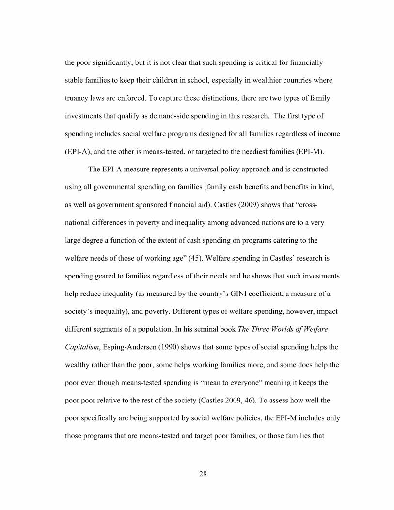
significant impact on poverty in less developed countries. Figure II-1 shows the

relationship between the EPI-A (2006) and the 2010 GINI coefficient for the countries

included in this dissertation. These are significantly and positively correlated (p=.04) and

shows simply that the countries in this dataset that spend more on supply relative to

demand have higher inequality.7 The level of a country’s wealth in all regression

analyses show that wealthier countries in the dataset have a slightly lower GINI

coefficient but this is due to the large number of European democracies included in the

sample.

7 There is not a causal relationship between the balance of supply-side and demand-side spending in 2006 for countries in this dataset and the countries’ 2010 GINI coefficient.

30

Figure II–1. EPI-A and GINI Coefficient

Tables II-3 and II-4 show the 33 countries that are included in the analyses

throughout Chapters II, III and IV of this dissertation. The countries’ EPI-A and EPI-M

scores for 2006 are presented along with a breakdown of the EPI’s spending categories.

There is some variation in the EPI-M scores but overall they are highly skewed to the

supply-side range of the index because so many countries included in this analysis are

wealthy and target their benefits to the broader population. The demand- and supply-side

spending percentages represent the percent of total EPI-A or EPI-M spending that is

allocated to each category. In Chapter III the political and economic reasons for these

country’s EPI-A and EPI-M scores will be examined in greater detail.

31

Table II–3. Country EPI-A Scores, 2006

% Supply Spending, EPI-A % Demand Spending, EPI-A*

Country EPI-A, 2006

% of EPI-A Benefits are Means-tested

Compensation School

Services Capital

expenditures Cash

Benefits Benefits in

Kind Financial

Aid

Australia 0.57 19% 40% 11% 6% 32% 10% 2% Austria 0.57 4% 43% 13% 2% 35% 7% 0% Belgium 0.60 4% 52% 7% 2% 24% 14% 1% Brazil 0.59 100% 41% 15% 3% 6% 35% 0% Canada 0.76 16% 56% 16% 4% 21% 3% 0% Chile 0.80 23% 80% 11% 9% 0% Czech Republic

0.62 33% 35% 22% 6% 24% 12% 3%

Denmark 0.52 13% 38% 11% 3% 18% 24% 6% Estonia 0.93 69% 93% 3% 1% 3% Finland 0.56 7% 33% 17% 5% 23% 20% 2% France 0.55 25% 41% 10% 5% 20% 24% 2% Germany 0.57 14% 45% 8% 4% 24% 17% 2% Hungary 0.48 6% 48% 32% 18% 2% Iceland 0.63 28% 44% 12% 7% 14% 22% 1% Ireland 0.52 11% 39% 8% 5% 36% 9% 3% Israel 0.66 14% 47% 15% 4% 16% 17% 1% Italy 0.70 32% 56% 11% 3% 13% 16% 1% Japan 0.76 38% 60% 8% 7% 12% 12% 0% Korea 0.86 17% 56% 21% 9% 0% 12% 1% Mexico 0.73 55% 66% 5% 2% 7% 15% 4% Netherlands 0.61 12% 44% 9% 9% 11% 23% 5%

32

Table II-3, continued

% Supply Spending, EPI-A % Demand Spending, EPI-A*

Country EPI-A, 2006

% of EPI-A Benefits are Means-tested

Compensation School

ServicesCapital

expenditures Cash

Benefits Benefits in Kind

Financial Aid

New Zealand 0.56 53% 56% 32% 10% 3% Norway 0.54 25% 37% 10% 7% 21% 20% 5% Poland 0.71 22% 58% 7% 6% 20% 7% 2% Portugal 0.74 42% 68% 4% 1% 16% 9% 1% Slovak Republic

0.95 53% 62% 29% 4% 2% 0% 2%

Slovenia 0.43 66% 31% 8% 4% 14% 6% 37% Spain 0.65 32% 48% 11% 6% 13% 20% 1% Sweden 0.52 13% 34% 14% 4% 20% 24% 3% Switzerland 0.71 18% 55% 10% 6% 21% 7% 1% Turkey 0.97 85% 79% 12% 6% 2% 0% 2% UK 0.53 15% 37% 10% 5% 31% 16% 1% USA 0.84 94% 60% 15% 10% 3% 13% 0%

* For some countries, even if the country allocates some monies to a supply-side category, it appears as 0% due to rounding. For example, Korea does spend some money on Cash Benefits for families, but it is a significantly small amount relative to the spending allocated to the other categories. SOURCES: OECD SOCX Database (2012b) and OECD Education Database (2012a). In addition, the following sources are used: a) For Brazil: Data for the Conditional Cash Transfer program, Bolsa Familia, as well as social assistance spending (the Social Assistance Reference Centres or CRAS and the Comprehensive Famiy Care Programme or PAIF) were available from Soares 2012, Soares et al. 2010, and Lindert et al. 2007. Social assistance estimates are calculated as 1.4% GDP (2005) or US$1.7 trillion. b) For Chile: Guardia et al. 2011, Fiszbein and Schady 2009, and OECD 2011d c) For Turkey: Sources confirming OECD financial aid spending (the country's spending on its Conditional Cash Transfer program) include: Şener 2012 and Rawlings and Rubio 2005, 35 (Table 2)

33

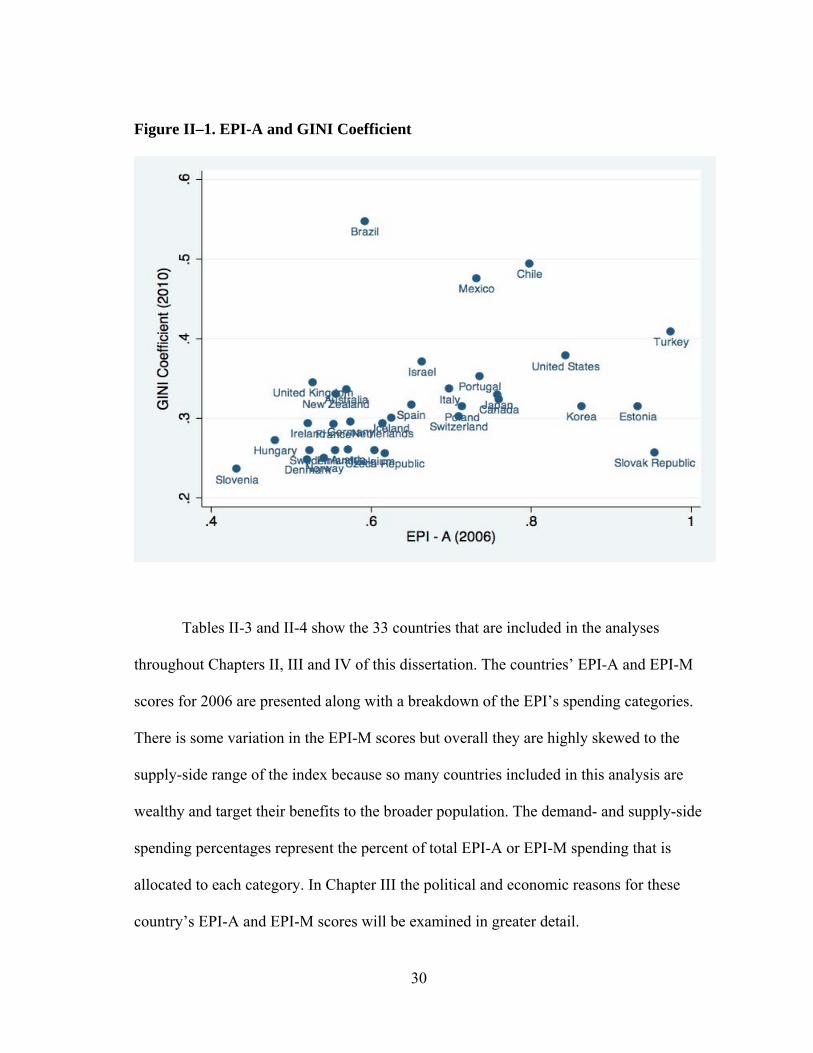
Table II–4. Country EPI-M Scores, 2006

% Supply Spending (EPI-M) % Demand Spending, EPI-M*

Country EPI-A 2006

EPI-M, 2006

Compensation School

Services Capital

expenditures Cash


Kind Financial

Aid

Australia 0.57 0.87 62% 17% 9% 0% 10% 3% Austria 0.57 0.97 72% 22% 3% 0% 2% 1% Belgium 0.60 0.98 84% 11% 3% 0% 0% 2% Brazil 0.59 0.59 41% 15% 3% 6% 35% 0% Canada 0.76 0.94 69% 20% 5% 0 6% 0 Chile 0.80 0.94 94% 5% 0% 1% Czech Republic 0.62 0.83 46% 29% 7% 14% 0 3% Denmark 0.52 0.89 65% 19% 6% 0% 0 10% Estonia 0.93 0.95 95% 1% 0 3% Finland 0.56 0.95 57% 29% 9% 1% 1% 3% France 0.55 0.83 62% 14% 7% 1% 12% 3% Germany 0.57 0.91 71% 13% 6% 5% 0% 4% Hungary 0.48 0.94 93% 2% 0% 4% Iceland 0.63 0.86 60% 16% 10% 9% 4% 1% Ireland 0.52 0.91 68% 14% 9% 4% 0 5% Israel 0.66 0.93 67% 21% 6% 1% 5% 1% Italy 0.70 0.88 70% 14% 4% 9% 2% 1% Japan 0.76 0.89 71% 10% 8% 0 11% 0% Korea 0.86 0.97 64% 23% 10% 0 1% 1% Mexico 0.73 0.83 75% 6% 2% 8% 4% 5% Netherlands 0.61 0.93 66% 14% 13% 0 0 7%

34


% Supply Spending (EPI-M) % Demand Spending, EPI-M*

Country EPI-A 2006

EPI-M, 2006

Compensation School

Services Capital

expenditures Cash


Kind Financial

Aid

New Zealand 0.56 0.70 70% 18% 8% 4% Norway 0.54 0.83 57% 15% 10% 0 10% 7% Poland 0.71 0.92 74% 9% 8% 6% 0 2% Portugal 0.74 0.87 81% 5% 1% 10% 2% 1% Slovak Republic

0.95 0.98 63% 30% 4% 0% 0% 2%

Slovenia 0.43 0.54 39% 10% 5% 0% 0% 46% Spain 0.65 0.85 63% 14% 8% 4% 8% 2% Sweden 0.52 0.90 59% 24% 6% 0% 5% 6% Switzerland 0.71 0.93 72% 13% 8% 1% 5% 1% Turkey 0.97 0.98 80% 12% 6% 0% 0% 2% UK 0.53 0.88 62% 17% 9% 0% 10% 2% USA 0.84 0.85 61% 15% 10% 3% 12% 0

* For some countries, even if the country allocates some monies to a supply-side category, it appears as 0% due to rounding. For example, Korea does spend some money on Cash Benefits for families, but it is a significantly small amount relative to the spending allocated to the other categories. SOURCES: OECD Education Database (OECD 2012a) and OECD SOCX Database (OECD 2012b). In addition, the following sources are used: a) For Brazil: Data for the Conditional Cash Transfer program, Bolsa Familia, as well as social assistance spending (the Social Assistance Reference Centres or CRAS and the Comprehensive Famiy Care Programme or PAIF) were available from Soares 2012, Soares et al. 2010, and Lindert et al. 2007. Social assistance estimates are calculated as 1.4% GDP (2005) or US$1.7 trillion. b) For Chile: Guardia et al. 2011, Fiszbein and Schady 2009, and OECD 2011d c) For Turkey: Sources confirming OECD financial aid spending (the country's spending on its Conditional Cash Transfer program) include: Şener 2012 and Rawlings and Rubio 2005, 35 (Table 2)

35

The countries presented in Tables II-3 and II-4 were selected because they

participated in the 2009 PISA exams and because their spending data are available in the

UNESCO/OECD /Eurostat (UOE) and OECD Social Expenditures (SOCX) databases.

Furthermore, there is a strong literature about these country’s education systems on

which this study can build. For three countries, though, data beyond the databases have

been needed. Brazil, Chile, and Turkey are upper middle income countries according to

the World Bank and additional budget information had to be added to reflect the impact

of conditional cash transfer programs and other spending initiatives not accounted for in

the databases. These countries receive international monies to help their social and

education programs and accounting for their expenditures is consequently more

complicated.

Most of the countries in the sample (20) are considered high income and the

remaining 13 countries are considered upper-middle income countries.8 Table II-5 shows

the GDP and GNI per capita for each participating country as well as the per-pupil

spending estimates based on supply-side spending (the traditional per pupil estimates),

EPI-A spending, and EPI-M spending.

8 “High income for nonOECD” is defined by the World Bank (World Development Indicators, 2009) as having a 2006 GDP per capita greater than $21,009 or a 2006 GNI per capita greater than $30,846.

36

Table II–5. GDP and GNI Per Capita (2006) and Per-Pupil Spending for Primary

and Secondary Public and Government-Dependent Private Schools, 2006

Country GDP per

capita (2006)

GNI per capita (2006) Spending Per Pupil (2006)

Supply-Side Only EPI-A EPI-M

Norway* $72,960 $53,330 $14,562 $26,885 $17,637

Iceland $54,814 $33,780 $13,023 $20,822 $15,181

Switzerland $54,140 $42,510 $12,167 $17,142 $13,073

Ireland $52,501 $37,270 $9,318 $17,885 $10,288

Denmark $50,462 $36,700 $13,310 $25,563 $14,912

United States $44,623 $45,640 $10,540 $12,499 $12,374

Sweden $43,949 $36,140 $9,677 $18,487 $10,810

Netherlands $41,459 $39,070 $8,440 $13,738 $9,072

United Kingdom $40,481 $35,150 $8,992 $17,040 $10,232

Finland $39,487 $33,430 $8,617 $15,514 $9,085

Austria $39,300 $36,110 $10,389 $18,179 $10,701

Canada $39,250 $36,410 $8,600 $11,314 $9,140

Belgium $37,919 $34,490 $8,313 $13,755 $8,518

Australia $35,986 $33,010 $6,512 $11,446 $7,451

France $35,457 $31,950 $8,727 $15,786 $10,473

Germany $35,238 $34,210 $6,422 $11,177 $7,096

Japan $34,102 $32,770 $8,224 $10,846 $9,214

Italy $31,777 $30,170 $8,865 $12,700 $10,090

Spain $28,025 $29,810 $5,257 $8,086 $6,153

New Zealand $26,173 $25,230 $5,184 $9,324 $7,392

Israel $20,625 $24,840 $4,393 $6,621 $4,708

Korea, Rep. $19,676 $24,320 $4,851 $5,621 $4,983

Slovenia $19,406 $25,140 $5,704 $13,190 $10,632

37


Country GDP per capita

(2006) GNI per capita

(2006)

Spending Per Pupil (2006) Supply-Side

OnlyCount

ry GDP per capita

(2006)

Portugal $19,065 $22,180 $5,189 $7,052 $5,967

Czech Republic

$14,446 $21,230 $2,890 $4,683 $3,484

Slovak Republic

$12,799 $17,800 $1,723 $1,805 $1,766

Estonia $12,503 $18,150 $2,659 $2,848 $2,790

Hungary $11,174 $17,300 $2,567 $5,344 $2,739

Chile $9,376 $11,380 $1,182 $1,481 $1,252

Poland $8,958 $14,680 $1,689 $2,366 $1,838

Mexico $8,831 $13,070 $1,356 $1,853 $1,628

Turkey $7,687 $12,790 $754 $773 $770

Brazil $5,793 $8,810 $940 $1,587 $1,587

*Countries are listed in order of wealth based on GDP per capita (2006). SOURCES: World Bank’s World DataBank World Development Indicators (WDI) and calculations based on EPI spending allocations. Enrollment numbers are based on those used in Table 1 from the OECD Education Database, dataset: students enrolled by type of institutions.

The traditional per pupil estimates do not include demand-side cash benefits or

benefits in-kind though they may include financial aid; for primary and secondary school

students, however, financial aid is minimal.9 The cash benefits that would be included in

some country’s educational spending stem from conditional cash transfer programs that

have become popular in developing countries. Mexico, Chile, Turkey, and Brazil each

have a form of this program that essentially pays families to send their students to

school. In Chapter III these countries’ decisions to pursue these programs will be

detailed but it is worth noting here that these spending decisions are mostly due to the

9 Data for spending per pupil is often separated by school level because upper secondary school spending per pupil is greater than lower secondary school spending per pupil that is in turn greater than primary school spending per pupil. Since overall education expenditures are being evaluated in this analysis for students through the secondary school level, this spending is aggregated. Future analysis could look at spending disaggregated by school level.

38

priority poverty reduction is for the party in power and the level of poverty each country

is trying to alleviate.

Section 2.4. Using the EPI as a Spending Indicator

The Program for International Student Assessment (PISA) has developed an

index for capturing the socio-economic status (SES) of students taking the PISA exams.

The PISA Index of Economic, Social, and Cultural Status (ESCS) is a “comprehensive

measure of student socio-economic background. This index was derived from

information comprising the highest educational level of parents, the highest occupational

status of parents, and possessions in the home” (OECD 2009a). Each country has a mean

ESCS score that shows the average SES of the students who took the 2009 PISA exam

relative to the average OECD student’s SES; the mean ESCS for each country used in

this dissertation is listed in Table II-6. The PISA coordinators make it a point to test a

representative group of students from each participating country’s population and the

ESCS scores reflect the GDP per capita very closely.

39

Table II–6. Average Economic, Social, and Cultural Status (ESCS) Index Mean by

Country, 2006

Country ESCS Mean Australia 0.34 Austria 0.06 Belgium 0.2 Brazil -1.16 Canada 0.5 Chile -0.57 Czech Republic -0.09 Denmark 0.3 Estonia 0.15 Finland 0.37 France -0.13 Germany 0.18 Hungary -0.2 Iceland 0.72 Ireland 0.05 Israel -0.02 Italy -0.12 Japan -0.01 Korea -0.15 Mexico -1.22 Netherlands 0.27 New Zealand 0.09 Norway 0.47 Poland -0.28 Portugal -0.32 Slovak Republic -0.09 Slovenia 0.07 Spain -0.31 Sweden 0.33 Switzerland 0.08 Turkey -1.16 United Kingdom 0.2 United States 0.17

40

To examine more closely how school and family spending impact a population of

students, the EPI-A can quickly show how countries with poorer (or wealthier) students

are spending their resources. Figure II-2 is a scatterplot that shows the 2006 EPI-A score

of each country relative to the mean 2009 ESCS index score of the students in each

country.10

Figure II–2. EPI-A Scores and Mean Student ESCS Scores by Country

Pairwise Correlation is negative and significant (p<.05) SOURCE: 2009 PISA 10 A three year lag is used throughout this dissertation between government expenditures (2006) and student outcomes such as assessment results and resilience scores (2009). The lag is to account for the time it takes for spending to have an impact on students. In all but a handful of countries there is not a great deal of variance in spending between 2006 and 2009. Those countries that have significant expenditure variation will be discussed in more detail in Chapter III.

41

The pairwise correlation between the EPI-A and the ESCS is negative and

significant (p<.05), and the pairwise correlation between the EPI-M and the ESCS is

insignificant, indicating then when only means-tested demand-side spending is

considered, there is no relationship between the average wealth of the students and the

balance of supply- and demand-side spending. The EPI-A result indicates that when a

country’s average student is poorer relative to the average OECD student, the country

spends more proportionally on school quality than on school access. The correlation also

implies that when students are wealthier (come from wealthier countries) they spend

more on demand-side or access policies. This may reflect the influence of the European

country’s relatively generous social polices.

What would be interesting to explore is what the ESCS is of each country’s

school-aged population (not just those taking the PISA exam) and to see if more poor

students are making their way into the school system given the country’s EPI-A score. If

a country is investing in demand-side policies and there are more poor students in

school, especially in countries where truancy laws are not strongly enforced, this would

indicate that the demand-side spending is achieving its goal of getting students to school.

The increased spending on schools when the students are less wealthy may be

reflecting an increased commitment to the students who are already there or to programs

designated for struggling students. One approach to further understand spending relative

to student wealth is to unpack the EPI-A.

42

EPIAc = 0+ ESCSc1 + eq. 2.2a EPIMc = 0+ ESCSc1 + eq. 2.2b

In the model above, EPIAc and EPIMc represents the six different EPI categories

for each country, and ESCSc is the mean ESCS score for each country.11 The GDP per

capita for each country is not used in the analysis because the ESCS scores already

capture the general wealth of the country.12 Results are shown in Table II-7 and show

that in the 33 countries studied, when the average student is wealthier, spending on

teacher compensation is proportionately less than spending on the other education

categories, and proportionately more is spent on cash benefits; accordingly, when

students are not as wealthy, countries are spending proportionately more on teacher

compensation and less on cash benefits. When only means-tested demand-side policies

are included in the analysis, the two spending categories of significance are school

services and capital expenditures – as the average family wealth of the students increase,

so do investments in these areas. The results indicate that when demand-side spending

targets only poorer students and their families, and when the average student in a country

comes from a less wealthy family, proportionately less money is actually going to the

school and infrastructure.

11 In Equation 2.2a, EPIAc represents the six categories of the EPI based on total demand- and supply-side spending estimates: the percent teacher compensation - A, percent school services-A, percent capital expenses-A, percent cash benefits-A, percent benefits in kind-A, and percent financial aid-A. In Equation 2.2b, the EPIMc represents the six categories based on total means-tested demand-side spending only plus supply-side spending estimates: the percent teacher compensation - M, percent school services-M, percent capital expenses-M, percent cash benefits-M, percent benefits in kind-M, and percent financial aid-M. 12 Because they did not disaggregate their spending data in the OECD database, Chile, Hungary, New Zealand, and the Slovak Republic are excluded in this analysis so N=29.

43

Table II-7. Relationship Between Student Wealth and Expenditures

Dependent Variables

Correlation of percent EPIAc categories with Mean ESCS

Correlation of percent EPIMc categories with Mean ESCS

Supply-Side Spending Percent Teacher Compensation

-.134 *** (.04) -.003 (.04)

Percent School Services

.010 (.02) .054* (.02)

Percent Capital Expenditures

.011 (.01) .03** (.01)

Demand-Side Spending Percent Cash Benefits

.095** (.04) -.021 (.02)

Percent Benefits in Kind

.005 (.03)

-.035 (.03)

Percent Financial Aid

.009 (.03) .017 (.03)

N=29, *p<.05, **p<.01, ***p=.01 NOTES: Standard errors in parentheses

Since most of the wealthier countries in this analysis have generous social

spending policies, this drives the results for the proportionately higher cash benefit

spending. The higher percentage of money going to teacher compensation when the

average wealth of students is lower could reflect a stronger commitment to the most

needy students. Such spending could reflect the hiring of more teachers, an increase in

teacher pay, or both, and any of these options could help students, so long as they were

getting to school in the first place. With a lower percentage of education monies going to

cash benefits, though, this may not be the case. Indeed, since we know the proportion of

spending on teachers is higher than the proportion of cash benefit allocations when the

44

average student is less wealthy, it is more likely that poorer students are not benefitting.

This suggests that money going to the schools is helping the students already there rather

than helping the students in need when the students come from families with income

below the OECD average.

If this is true, then are students who come from less wealthy families, benefitting

from school spending? Based on the 2009 PISA exam results in reading, the OECD was

able to determine how resilient students are in each country taking the exam. “A student

is classified as resilient if he or she is in the bottom quarter of the PISA index of

economic, social and cultural status (ESCS) in the country of assessment and performs

in the top quarter across students [in reading] from all countries after accounting for

socio-economic background” (OECD 2010b, 63). Table II-8 shows the resilience of

students from each country on the reading exam, listing the most resilient countries first.

Korea, Finland, Japan, and Turkey, in that order, have the most resilient students.

45

Table II–6. Student Resilience on the 2009 PISA Exams

Country % Resilient students from

the country's poorest Korea 56% Finland 46% Japan 42% Turkey 42% Canada 39% Portugal 39% Poland 37% New Zealand 37% Spain 36% Estonia 34% Netherlands 32% Italy 32% Switzerland 32% Australia 31% France 30% Belgium 30% Ireland 30% Iceland 29% Mexico 29% United States 29% Norway 26% Hungary 26% Sweden 25% Slovenia 25% Chile 24% Denmark 24% Israel 24% United Kingdom 24% Germany 23% Brazil 22% Czech Republic 21% Slovak Republic 21% Austria 20%

SOURCE: PISA 2009 Database (OECD 2010c)

46

To begin to understand the role spending has had on student resilience, Figure II-

3 shows the EPI-A score of each country and the resilience of the students in that

country. A simple correlation between the EPI-A and student resilience is positive and

significant (p=.03) indicating that as countries invest proportionally more in schools,

they are improving the scores of at least some of the neediest students in reading.

Figure II–3. EPI-A Scores and Student Resilience

NOTE: Percent of Resilient Students are the percent of students from the bottom quartile on the PISA Economic, Social, and Cultural Status (ECSC) index who were top performers on the 2009 PISA Reading exam. SOURCE: Education at a Glance 2011a (OECD)

47

Given these results, school spending does appear to be helping the poor students

rather than just the wealthy students who are already at school. Even if countries are

spending less on family cash benefits, when the students do get to the school, it appears

that they are making some gains thanks to the supply-side investments countries are

making.

Section 2.5. Conclusion

The all-encompassing Education Policy Index (EPI-A) has been carefully

constructed to include all the spending countries designate for public and government-

dependent private schools, as well as to families. Since the EPI-M only considers means-

tested programs, rather than more broadly oriented family programs, it could prove more

useful for analyzing less-developed countries or countries that have more means-tested

programs.

In addition to the overall EPI-A and EPI-M country scores, it is useful to know

the proportion of spending going to each of the six EPI categories in the same year. The

breakdown of each category makes it possible to analyze the broader, relative impacts of

spending allocation decisions. Policies do not happen in isolation and this breakdown

gives analysts the chance to consider what is simultaneously happening

programmatically for students at home and at school. For example, we saw that

proportionately more monies are going to compensate teachers than to giving families

cash benefits when countries have less wealthy students and that, based on student

resilience on the 2009 PISA reading exam, this spending appears to have a positive

48

impact on student outcomes. This strongly implies that spending on schools does make a

difference for students – money matters.

The utility of the country-level EPI-A and EPI-M scores will be explored

throughout the dissertation. EPI scores at state or regional levels, or even across schools

and districts, could also be conceived given the right dataset. When analyzing how

spending impacts individual students going to the same school, the EPI would not be

appropriate as there is no variation in the supply-side spending unless data are available

for spending allocations to different classrooms. In Chapter V of this dissertation, how

the benefits of particular social policies impact students from the same school is

addressed.

49

CHAPTER III

WHAT DO COUNTRY POLITICS TELL US ABOUT EDUCATION POLICY

INDEX SCORES?

Chapter II introduced the Education Policy Index (EPI) and the supply- and

demand-side spending that determines countries’ EPI-A and EPI-M scores. This chapter

explores countries’ political and economic conditions and evaluates how they impact

governments’ education and family-oriented policy and spending decisions. Wealthier

countries spend more on education overall as well as proportionally than less developed

countries (LDCs), with the United States being one of the few and notable exceptions.

Gross Domestic Product per capita (GDPpc) explains 16% of overall spending on

education and family-benefit policies, 15% of supply-side or education spending

policies, and 27% of all demand-side or family benefit policies; means-tested demand-

side policies are not explained by a country’s wealth.13

Wealth explains 14% of the EPI-A or the balance of all demand-side and supply-

side spending, but none of the EPI-M. These findings imply two things. First, means-

tested policies, or policies that target only the poorest based on their income, are not

determined based on the wealth of the country – they appear to be politically driven

13 Calculations are based on the adjusted R-square of four simple linear regression models with the independent variable being each country’s GDP per capita and the dependent variable being each country’s percent of GDP allocated (in turn) to supply and demand-side spending, supply-side spending only, demand-side spending only, and means-tested demand-side spending only.

dec

cou

fac

cou

cap

cha

inf

cou

Fig

cisions. Seco

untry is willi

ctors should b

This ch

untries vary

pital develop

apter discuss

form how mu

untries’ expe

gure III–1. T

Pol• Electo• Labor

Stren• Intera

Syste

Ideolog

• Stren• Appr

c

Lev• Politi• Civil

ond, though

ing to spend

be considere

hapter explor

in their polic

pment and ec

ses in detail.

uch countrie

enditures can

The Conditi

litical Instituoral System (r Organizatiogth action - Electoem and Labor

gy of Ruling Coalition

ngth of the Leroach to welfacapitalism

vel of Democical Rights Liberties

a country’s w

on these po

ed.

res the politi

cy expenditu

conomic gro

By examini

s invest in fa

n be better u

ional Model

Economic D• GDP pe• Income

tions (PR) on

oral Strength

Party or

eft fare

cracy

50

wealth expla

licies, it is o

cal and insti

ures. Figure

owth model p

ing the politi

amilies and e

understood.

l of Human

Developmener capita Equality and

EdFamEx(E

PoS

De

ains a fair am

only part of t

itutional com

III-1 presen

presented in

ical and inst

education, th

n Capital De

nt

d Poverty

ducation and mily BenefitxpendituresEducation olicy Index) Supply and emand-side Spending

mount of how

the story and

mponents tha

nts the part o

Figure I-1 th

titutional com

he difference

evelopment

w much a

d the politica

at impact wh

f the human

hat this

mponents tha

es between

al

hy

at

51

Theories of redistribution built around government ideology, countries’ electoral

systems, and the strength of unions as well as countries’ commitment to civil liberties

and political rights, are explored in the analysis presented in this chapter. Left leaning

parties, proportionally representative election systems (PR), and the strength of unions

explain a great deal of the variation in the way countries spend on education and family

benefits. The findings show that more left leaning systems and governments that have

both a PR system and strong unions, will provide more benefits to families. Moreover, as

will be discussed in Chapter IV, these policies in turn impact a country’s level of social

and human capital that ultimately impedes or supports a country’s economic growth.

Section 3.1 discusses the political science and sociology literature that addresses

government redistribution policies and how they relate to education and family-benefit

expenditures. Section 3.2 puts the policy expenditures into a budgetary context, and

Section 3.3 addresses how the institutional factors influence the level of country

expenditures on such policies. A model for testing the theoretical factors is presented

and analyzed in Section 3.4.

Section 3.1. The Redistributive Nature of Education and Family-Benefit Policies

Both education and family-benefit policies are social in nature because they

“address social problems and/or provide employment supports” (Adema 2006, 14). In

the literature on welfare and social spending, however, education is not always included.

Iversen and Stephens (2008) argue that this is a mistake. “Skills and education are at the

core of the welfare state. Incentives to acquire particular types of skills are closely

52

related to both social protection and economic performance, and educational spending is

not only a partisan issue but also one with profound implications for the distribution of

income” (Iversen and Stephens 2008, 602). As a social policy, education does provide a

universal good that any family, regardless of their income level, can use. As a

universally provided good, however, it is not necessarily redistributive.

Ansell (2010) has argued that education spending is redistributive only in so far

as “who actually receives that education” (3). University spending he explains can be

regressive since the wealthy more often take advantage of public higher education. In

primary and secondary schools, it is a bit more complicated when non-government

supported or managed private schools are taken into account. If wealthier families opt

out of public schools altogether then the redistributive nature of school spending would

be quite high. However, most countries’ primary and secondary public and government-

dependent private schools serve 90% or more of the school-aged population, so both rich

and poor are accessing this publically provided good at least to some extent (OECD

2012c, Table C1.4, 333). Iversen and Soskice (2009) claim definitively that spending on

primary and secondary schools “benefits low-income groups more than high-income

groups,” but this is not a certainty (454). Jensen (2011), who looks at overall education

spending at all grade levels, argues that so long as taxation is progressive, public

education will be redistributive but that spending on education is among the least

redistributive programs in which governments can invest. “It is even the case that high-

income groups use publicly provided education more than low-income groups because

full usage is conditioned on high levels of cultural capital, something that all else equal

53

favors high-income groups” (Jensen 2011, 413).14 Supply-side spending, spending on

education, therefore, is redistributive to some extent, but how redistributive is it relative

to demand-side spending or family benefit programs and financial aid?

Financial aid at the primary and secondary school level is means-tested and

targets children who come from families who are struggling economically. Means-tested

family benefits are policies designed to target only the poor as well; beneficiaries are

determined based on their economic need. These types of policies in the welfare capital

literature are considered “liberal” because they typify a laissez-faire approach to

governance – they minimize government involvement in marketplace outcomes; the

United States is often used as the prototype of this category. In this approach, the

government only steps in to assure a basic standard of living but keeps beneficiaries tied

to their market conditions – in Esping-Andersen’s (1990) terms, this keeps beneficiaries

commodified. A country’s welfare system in this literature is evaluated based on “the

degree to which a (social) service is rendered as a matter of right, and the degree to

which a person can maintain a livelihood without reliance on the market” (Arts and

Gelissen 2002, 141).

In his seminal work, The Three Worlds of Welfare Capitalism, Gøsta Esping-

Andersen (1990) introduces the three types of welfare capitalism: liberal, conservative,

and social-democratic. These categories are based on countries’ healthcare,

unemployment, sick leave, and poor relief policies, as well as pension schemes (Table

3.1, 70-1). The liberal regime’s approach to welfare is described above. The

14 Cultural capital here refers to the societal norms and knowledge children inherit from their parents or families; this includes going to school and pursuing higher education.

54

conservative welfare system is one that moderately tries to decommodify policy

beneficiaries but does so based on occupational groupings so that social benefits depend

on previous contributions. Countries such as Germany, Austria, France, Italy, and

Belgium most strongly fall into this category with their legacy of guilds and preferential

benefits to civil servants.

Social-democratic countries are those that offer policies that try to minimize the

commodification of its citizens. Mostly Scandinavian, the countries in this category

consider benefits to be a social right and provide universal benefits. Table III-1 lists

Esping-Andersen’s (1990) categories of countries and where they fall in this scheme.

Each country’s score in the capital welfare typology is based on a variety of

stratification indices. If a country has more than two pension schemes that are

occupationally based, for example, and if civil servants receive special consideration,

these countries receive a higher score on the conservative index; the conservative scale

also considers the percentage of pensions that are based on private funds. The liberal

scale is based on the percentage of all social benefits that are means-tested, and for the

social-democratic scale, scores are based on the percentage of the population that

benefits from a set of programs. When more than 86% of a population benefits from

social programs, the country scores high on the social-democratic scale, if less than 60%

of the population benefits, it scores low. The other consideration for the social-

democratic category is the average difference between the basic and maximum benefit

payouts for sickness, unemployment, and pensions.

55

Table III–1. Country Welfare Capital Scores

Degree of

Conservatism Degree of

Liberalism Degree of Socialism

Australia Weak (0) Strong (10) Medium (4) Austria Strong (8) Weak (4) Weak (2) Belgium Strong (8) Weak (4) Medium (4) Brazil N/A N/A N/A Canada Weak (2) Strong (12) Medium (4) Chile N/A N/A N/A Czech Republic N/A N/A N/A Denmark Weak (2) Medium (6) Strong (8) Estonia N/A N/A N/A Finland Medium (6) Weak (4) Strong (6) France Strong (8) Medium (8) Weak (2) Germany Strong (8) Medium (6) Medium (4) Hungary N/A N/A N/A Iceland N/A N/A N/A Ireland Medium (4) Weak (2) Weak (2) Israel N/A N/A N/A Italy Strong (8) Medium (6) Weak (0) Japan Medium (4) Strong (10) Weak (2) Korea (South) N/A N/A N/A Mexico N/A N/A N/A Netherlands Medium (4) Medium (8) Strong (6) New Zealand Weak (2) Weak (2) Medium (4) Norway Medium (4) Weak (0) Strong (8) Poland N/A N/A N/A Portugal N/A N/A N/A Slovak Republic N/A N/A N/A Slovenia N/A N/A N/A Spain N/A N/A N/A Sweden Weak (0) Weak (0) Strong (8) Switzerland Weak (0) Strong (12) Medium (4) Turkey N/A N/A N/A UK Weak (0) Medium (6) Medium (4) United States Weak (0) Strong (12) Weak (0)

*Adapted from Table 3.3 in Esping-Andersen (1990), 74

56

These categories have maintained a fair amount of traction in the twenty years

they have been applied and scrutinized in social science research (Arts and Gelissen

2002). Family benefits, however, are not explicitly included in the typology and this has

met with a variety of challenges (Sainsbury 1994).15 Some researchers have argued that

beyond the state and the market, the family has played a significant role in providing

welfare benefits such as caring for the elderly and the young, and taking care of the

women who are usually charged with such responsibilities (Bryson, et al. 1994). As

women have challenged traditional gender roles and have become incorporated into the

formal labor market, as they have become more commodified, their role in society has

changed. Accordingly more benefits are needed to assist women who now need to take

time away from work to give birth, as well as care for young children or elderly family

members (Siaroff 1994, Trifiletti 1999). Men also need to receive such benefits as they

are now expected to share in parenting and care-taking obligations, thus these benefits

are considered family benefits.

Trifiletti (1999, 54) argues that depending on how a system integrates women

into the workforce and provides for their families, there are actually four types of

welfare regimes: 1) liberal and 2) universalist (these minimize gender discrimination and

consider women part of the workforce), and 3) breadwinner and 4) Mediterranean (these

maximize gender discrimination and reinforce women’s roles as wives and mothers

rather than as part of the workforce). Liberal and Mediterranean regimes are seen to

15 Neyer and Andersson (2008) argue that the Esping-Andersen (1990) typology does not work when evaluating “the effect of family policies on fertility and childbearing behavior” (706). Since this dissertation and this chapter in particular is concerned with spending and not reproductive decisions, Neyer and Andersson’s concerns are not addressed.

57

leave women unprotected from the market whereas breadwinner policies such as those in

Germany and Ireland, and universalist policies such as those in Sweden, protect women

from market forces.

The breadwinner regimes, according to Trifiletti, include those countries in

which women receive benefits through their husbands and mostly work part-time. Since

they are protected as wives and mothers in these countries, Trifiletti argues that women

are subsequently protected from the market. She is incorrect on two fronts. First, married

women are tied to the market through their husbands. Second, for women who are not

married and work full time, their social benefits are tied to their income, so they also do

not escape the market. This makes those countries in the breadwinner category very

similar to those in the Mediterranean one since the market plays a significant role in

determining the level of women’s benefits. Moreover, the women in breadwinner and

Mediterranean countries are generally expected to fulfill the child and elder care

responsibilities of the extended family. Thus, in both categories women’s benefits are

determined more from their role as daughters, sisters, wives, or mothers than they are by

the labor market. Trifiletti’s distinction between breadwinner and Mediterranean regimes

then, appears to be a false dichotomy and countries in these categories could better be

understood using Esping-Andersen’s market-based conservative typology that also takes

into consideration how women’s roles are understood by society.

As described earlier, conservatism is tied to how much countries differentiate

non-means-tested payments between beneficiaries. Applying Trifiletti’s typology to

Esping-Anderson’s three worlds of welfare capitalism means considering not just the

58

market and payment differentials, but also how women are treated by social policies.

Countries that consider women to be workers who are tied to the market (just as men

are) would be considered liberal or universal, and those that consider women based on

their family roles are conservative. Since the benefits discussed in this dissertation center

around the family, how these specific benefits fit into Esping-Andersen’s scheme merits

further discussion.

Table III–2. Family Benefits Up Close and Personal

Cash benefits Family allowances

Family or child tax benefits Parenting payment (Single and Partnered) Single Income Family Bonus Back to School Bonus Family support (egalitarian benefits) Conditional Cash transfer benefits

Maternity and parental leave Maternity/parental leave benefit

Income maintenance benefit in the event of childbirth Parental leave benefits

Other cash benefits Partner allowance

Benefits in kind Day care / Home-help services

Home help Child day care

Other benefits in kind Services for families with children

Family and child welfare

59

Table III-2 profiles the family benefits considered part of the demand-side

spending that is central to the EPI-A and EPI-M. The benefits listed are a broad

summary of those offered in the 33 countries included in the dataset used throughout this

dissertation; the second level categories come from the sub-categories used in the

Organization for Economic Co-Operation and Development (OECD) Social Expenditure

Database (SOCX). Cash Benefits/family allowances are designed to keep families out of

dire straits when they grow and usually increase depending on the number of children

that are part of the legally recognized family unit; in some countries (e.g., Australia and

South Korea) there are additional monies for families that are single income. Income

maintenance is the priority of maternity/parental benefits. These exist for families in

which the mother and/or father has been working and is often not available unless the

parent has been working for a minimal period of time. Family Benefits in Kind are tied

to day care and home help in the case of caring for the elderly.

These benefits are highly variable across countries. For those benefits that are

mean-tested, they can be categorized as liberal since they are always market-based, treat

men and women as workers, and are as minimal as possible for families in need – they

are not designed to secure a middle class level of income for recipients. Family benefits

that would be considered conservative are market-driven in so far as they are determined

by past income and do not guarantee a family wage. Further, they primarily consider

women in their gendered roles rather than as equal members of the labor force. Lastly,

the Scandinavian or universalist (social-democratic) regimes treat women as workers

and protect them from the market as much as they would their male counterparts.

60

To summarize, for the purposes of this dissertation, countries that are considered

universalist are likely to invest more heavily in family or demand-side benefits than in

education to decommodify its population. Liberal regimes with their market-driven

approach to welfare, will invest more in education, and conservative regimes will be a

bit more generous to family and students than liberal regimes but would be expected to

invest more heavily in education (supply-side policies).

Hypothesis 3.1: Countries that are considered liberal welfare regimes will allocate more resources to schools (supply-side policies) than to family or student benefits (demand-side policies); conservative regimes will allocate funds a bit more evenly whereas universalist regimes will devote more resources to demand-side policies.

Liberal and conservative regimes do not guarantee that the level of family

benefits they provide will keep children from poverty; reliance on the market to

determine payments keeps a portion of the population poor. When family benefits are

paid in these regimes then, since they are means-tested, they should be considered highly

redistributive since they are explicitly targeting a country’s most needy families. Family

benefits in universalist regimes would appear to be more redistributive than those in the

conservative or liberal regimes since the benefit amounts are intended to minimize

inequalities and keep everyone at a middle or higher income level. However, these

countries tend to be wealthier to start with and have less overall poverty. Consequently

these payments are not as redistributive as those in conservative and liberal regimes. In

the aggregate though, family benefits are considered more redistributive given their

family-orientation and poverty targeting than education or supply-side spending.

61

Therefore, throughout this dissertation, countries that spend more on family benefits than

education will be considered to have more redistributive policies.

Section 3.2. How Much of the Budget Are We Talking About? Nations’ Education

and Demand-Side Policy Choices

Figure III-2 shows countries’ supply-side spending, expenditures on primary and

secondary schools, as a percentage of GDP relative to each country’s means-tested and

universal demand-side (family benefits and financial aid) spending. The country with the

most generous education spending for primary and secondary schools in this sample, at

4% of GDP, is Denmark, followed by Israel, Slovenia, Sweden, Belgium, Australia, and

New Zealand. All of these countries except for Israel are more evenly balanced in their

supply and demand-side spending proportions and have an EPI-A of .60 or less (Israel

has an EPI-A of .66). Slovenia (10%), Denmark (9%), Iceland (8%) and Sweden (8%)

have the highest overall spending on education and family-oriented social programs as a

percent of GDP – indicative of their egalitarian, universal policy orientation.

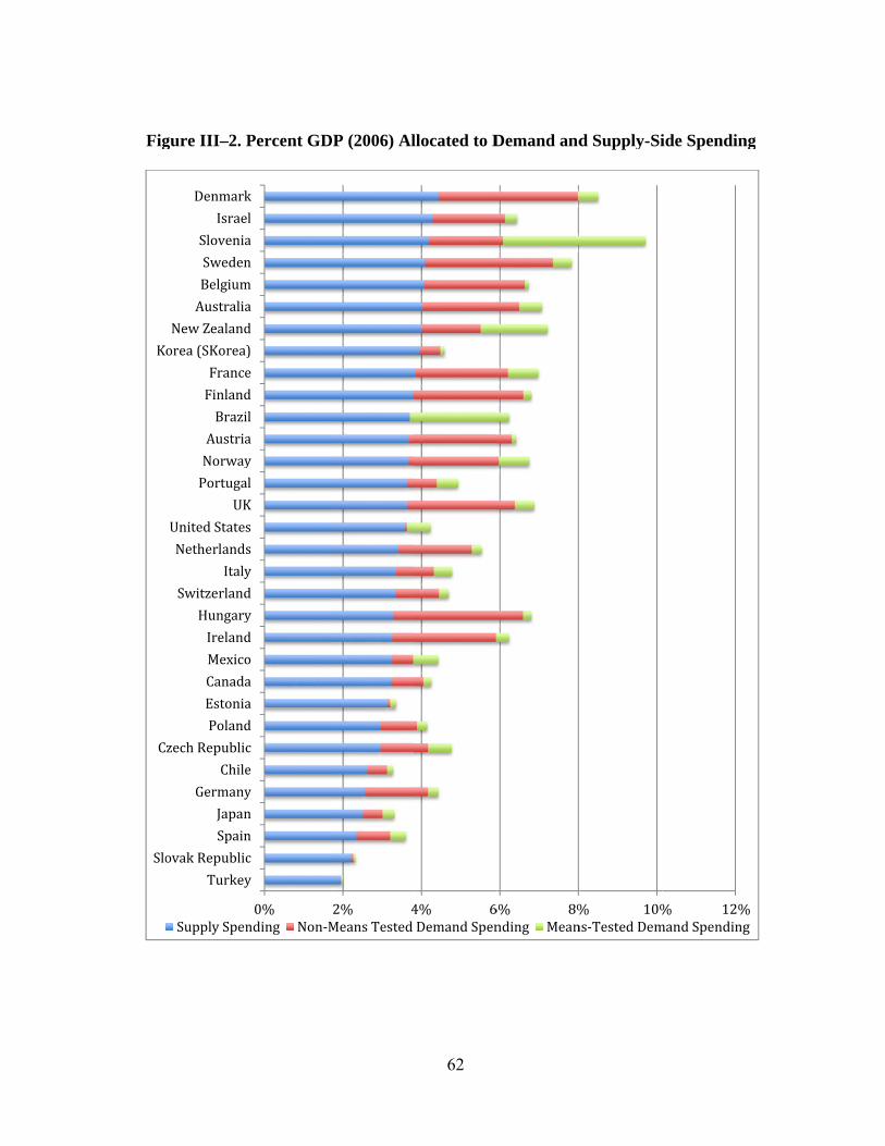
Fig

Slo

C

K

gure III–2. P

Turkey

ovakRepublic

Spain

Japan

Germany

Chile

zechRepublic

Poland

Estonia

Canada

Mexico

Ireland

Hungary

Switzerland

Italy

Netherlands

UnitedStates

UK

Portugal

Norway

Austria

Brazil

Finland

France

orea(SKorea)

NewZealand

Australia

Belgium

Sweden

Slovenia

Israel

Denmark

SupplySpen

Percent GD

0%

y

c

n

n

y

e

c

d

a

a

o

d

y

d

y

s

s

K

l

y

a

l

d

e

)

d

a

m

n

a

l

k

nding Non‐M

DP (2006) Al

2% 4MeansTested

62

llocated to D

4% 6DemandSpen

Demand and

6% 8%nding Mean

d Supply-Si

% 10%ns‐TestedDem

ide Spendin

% 12%mandSpending

ng

%g

63

Slovenia, formerly Yugoslavia, is noteworthy as a former Communist country in

that its transition to democracy and capitalism was introduced slowly and was less

disruptive than it was in most other post-socialist countries (Kolarič, et al. 2011). In

general Slovenia has low poverty and income inequality and has enjoyed economic

success. To live a comfortable middle class lifestyle, though, families require two full-

time working parents and the available family benefits reflect a commitment to working

women who have a long history of full-time employment in Slovenia (Stropnik and

Šircelj 2008). In terms of overall expenditures, Slovenia is the most balanced in its

supply- and demand-side spending priorities of all the countries in the dataset whether

looking at its EPI-A (.43) or EPI-M (.53) scores. This implies that most demand-side

spending is means-tested and it is based on the large amount of financial aid provided to

primary and secondary students; the family benefits portion of the demand-side

spending, however, is primarily universal.

While family benefits have been an important part of Slovenia’s expenditures

since before the transition to democracy, education reform and spending did not become

a high priority until the early 1990’s after Slovenia became independent. Starting in

1991 with the Law on Organization and Financing of Education, Slovenia reorganized

the education system and determined new rules for financing, increased spending, and

improved their enrollment numbers (Plut-Pregelj 2001). The spending on education

continued to increase as the country prepared to enter the European Union (EU) and

North Atlantic Treaty Organization (NATO) in 2004 and the balance between the two

types of spending in 2006 reflects these pattern. Hungary is similar to Slovenia in that its

64

spending between supply- and demand- is very balanced based on the EPI-A score,

however, most benefits in Hungary are universal so its EPI-M score is .93 or very

skewed to education spending.

Other countries in the dataset that had experience with Communism vary

considerably from Slovenia and Hungary. Formerly Czechoslovakia, the Czech Republic

and Slovakia today have two very different approaches to spending on education and

demand-side spending. The Czech Republic has an EPI- A score of .62 and an EPI-M

score of .83 indicating that most of the demand spending is universal (38% of demand-

spending is actually means tested) and that education spending is a comparable priority

to family-oriented social benefits. Slovakia on the other hand has the most supply-side

oriented EPI in the dataset with an EPI-A score of .95 and EPI-M score of .98. Here the

spending on means-tested student financial aid reflects 53% of the demand-side benefits

whereas the cash benefits and benefits in kind are primarily universal. This indicates that

education has been the priority for Slovakia, along with direct aid to students who are

going to school, and family benefits are designed to help everyone regardless of income.

Figures III-3 and III-4 show the EPI-A and EPI-M scores for all of the countries in the

dataset and indicate the median score (See also Tables II-3 and II-4 in Chapter II to see

how the scores break down along the spending categories).

Figure III–3

3. EPI-A Score

DenmaIre

0.5

0.55

0.6

0.65

0.7

0.75

0.8

0.85

0.9

0.95

1

es

arkelandSwedenUKNorway

FranceFinlaNewandZealandAustraliaAustriaGermany

BrazilBelgiNethCz

EPI

65

iumherlandsechRepublicIceland

SpainIsrael

ItaSwi

2006‐A

lyitzerlandPoland

MexicoPortugalJapanCan

U

Medi

nada

Chile

UnitedStatesKorea(SKorea)

EstoniaSlovakRep

Tur

ian=.6

publicrkey

Figure III–44. EPI-M Score

Slovenia

Brazil

NewZea

NoCze

0.5

0.55

0.6

0.65

0.7

0.75

0.8

0.85

0.9

0.95

1

es

aland

orwayechRepublicMexicoFranceUnitedStaSpaIctesainceland

PortugalAustraliaItalyUKJapD

EPI

66

panDenmarkSwedenGermanyIreland

PolanNetheSw

I2006‐M

derlandswitzerlandIsraelHungaryCanadaChilFin

Med

lenlandEstoniaAustriaKorea(SKoreaSlovakRepuBelgiT

dian= .89

a)ubliciumTurkey

67

The median EPI-A score for all countries in the dataset is .60 whereas the median

EPI-M score is .89. This disparity indicates that most countries in the sample provide

benefits that are more universally oriented and are not means-based. The countries with

the most 2006 means-tested demand-side policies are Brazil (100%), the United States

(94%), and Turkey (85%). The OECD shows that these countries’ 2010 Gini index or

inequality scores vary considerably: Brazil has a .55 Gini index score, Turkey an index

score of .41, and the U.S. a Gini index score of .38.16 While Brazil has a poverty rate of

21%, Turkey and the U.S. are not far behind with each having a 17% poverty rate. Table

III-3 shows the poverty rates and GINI scores for each country in the dataset. The only

countries with comparable poverty rates are Mexico (21%), Israel (20%), and Chile

(18%).17

16 With the exception of Brazil, the 2010 Gini index scores are from the OECD Country Statistical Profiles database; Brazil’s 2009 score comes from the World Bank (2009) database of World Development Indicators. The World Bank database defines the Gini index as “the extent to which the distribution of income (or, in some cases, consumption expenditure) among individuals or households within an economy deviates from a perfectly equal distribution. A Lorenz curve plots the cumulative percentages of total income received against the cumulative number of recipients, starting with the poorest individual or household. The Gini index measures the area between the Lorenz curve and a hypothetical line of absolute equality, expressed as a percentage of the maximum area under the line. Thus a Gini index of 0 represents perfect equality, while an index of 100 implies perfect inequality” (World Bank “World Development Indicators - Aggregated Database” 2009, OECD “Country Statistical Profiles Database” 2011e). 17 The poverty rates listed here are from the OECD “Country Statistical Profiles Database” 2011e and represent the poverty ratio from the late 2000’s. The poverty ratio is defined by the OECD 2010 Factbook as “The ratio of the number of people who fall below the poverty line and the total population; the poverty line is here taken as half the median household income. However, two countries with the same poverty rates may differ in terms of the income-level of the poor” (OECD 2010d, 236).

68

Table III–3. Country Poverty and GINI Scores

Country GINI Score Poverty Rate Brazil 0.55 21% Chile 0.49 18% Mexico 0.48 21% Turkey 0.41 17% USA 0.38 17% Israel 0.37 20% Portugal 0.35 12% UK 0.34 11% Italy 0.34 11% Australia 0.34 15% New Zealand 0.33 11% Japan 0.33 16% Canada 0.32 12% Spain 0.32 14% Estonia 0.32 12% Korea 0.32 15% Poland 0.31 10% Switzerland 0.30 9% Iceland 0.30 6% Germany 0.30 9% Netherlands 0.29 7% Ireland 0.29 9% France 0.29 7% Hungary 0.27 6% Austria 0.26 8% Finland 0.26 8% Sweden 0.26 8% Belgium 0.26 9% Slovak Republic 0.26 7% Czech Republic 0.26 5% Norway 0.25 8% Denmark 0.25 6% Slovenia 0.24 8%

NOTE: Countries with a poverty rate of 15% or greater are in bold. SOURCE: OECD “Country Statistical Profiles Database” 2011e

69

A closer look at how poverty rates are impacted by supply-side, means-tested,

and non-means-tested demand-side expenditures reveals that poverty is lower for the

countries in this dataset that spend more on non-means-tested demand-side policies.18 In

Chapter IV these decisions’ impact on educational outcomes will be addressed but first it

is important to identify which institutional factors influence the type of spending

countries prioritize. Accordingly, the next section addresses the key aspects of countries’

political institutions that help explain their EPI-A and EPI-M scores.

Section 3.3. Which Political and Ideological Factors Matter?

Democratic Political Institutions

Under democracies, governments provide more public goods and are more

redistributive than under authoritarian regimes (Przeworski, et al. 1999, Kaufman and

Segura-Ubiergo 2001, Lake and Baum 2001, Brown and Hunter 2004, Avelino, et al.

2005). Electoral systems in particular influence how generous governments will be once

they take control of a country’s budget. Democracies that elect their leaders via

proportional representation (PR) systems tend to be more redistributive than majoritarian

systems (Iversen and Soskice 2006, 2009). According to Iversen and Soskice (2006), the

reason for this leftist tendency in PR systems is that the middle class/centrist party can

ally with left-leaning parties and influence policy differently than in majoritarian 18 A linear regression model (with p =.002) was run with countries’ poverty rate as the dependent variable and the percent of spending on supply-, means-tested demand- and non-means-tested demand-side spending as the independent variables of interest. The only variable that was having an impact on reducing poverty was non-means-tested demand-side spending at p=.001. None of the other variables were significant including the GDP per capita control variable.

70

systems. In a PR system, the middle class can benefit more from taxation on the

wealthiest whereas in majoritarian systems the middle class will be included in higher

taxes if the left is in control of policy (166). Accordingly we would expect to see PR

systems spend more heavily on demand-side policies that are more redistributive than

education spending.

Hypothesis 3.2: Proportionally Representative (PR) Systems will spend relatively more than majoritarian systems on demand-side policies that are student and family-oriented than on supply-side policies that target schools and teacher wages.

The level of a country’s democratization is another component of how much a

country redistributes its wealth (Iversen and Soskice 2006, Iversen and Stephens 2008,

Iversen and Soskice 2009). Democratic countries that value citizens’ political rights and

civil liberties, would be expected to spend a great deal on education to assure an

electorate that can make rational voting decisions. Accordingly they will want to reach

as many constituents as possible and education is a way to reach families and garner

political support. David S. Brown and Wendy Hunter (2004) argue that “democratically

elected politicians would be especially likely to direct resources to the primary

[education] level, because such an approach would benefit the largest number of

potential voters” (845). In his analysis of democracies and their levels of education

spending, Ansell (2008) confirms that democratization increases primary education

spending.

Highly democratic countries are also expected to provide a safety net for its

population so that poorer citizens are not living in poverty and will support the

71

government (and vote for incumbents). Yet, redistributive spending should be geared

toward educating the populace for three reasons. First, as mentioned above, politicians

want to reach as many potential voters as possible and education is an easy way to do

that (family benefits primarily benefit the poor). Second, the work force needs to be

educated to provide a skill level that benefits the economy and third, an educated

electorate will be able to capably participate in the workings of government (Castelló-

Climent 2008; Iversen and Stephens 2008; Brady et al., 1995).

Hypothesis 3.3: More democratic countries will invest more in education (supply-side policies) than in family and student benefits (demand-side policies) to assure that citizens are able to participate in the economy as well as the running and monitoring of government.

Partisan Ideology, Labor Unions and Redistribution

Left-leaning governments have been found to be more distributive and

redistributive than those that are more conservative (Bardhan 2002). The ideological

position of the government can change each election and, provided the legislature and

the executive pass new laws, the policies they pass should reflect their ideological

preferences (Cusack 1997). The challenge with capturing such policies’ effectiveness,

however, is twofold. First, if the policy itself is meant to be more of a symbolic policy

than an implemented one, it may not get funding; budget allocation therefore is a key

part of this analysis. A second reason to include funding is that if a new administration

with a distinctly different ideological position from their predecessor is elected, the new

administration might increase or decrease the program’s budget. A new administration

72

might also reprioritize the bureaucratic effort by limiting funds to certain programs,

implementing a previously symbolic program, or overturning a policy altogether before

the policy’s impact can be measured. Partisan theory claims that “parties in power have

an impact on policy output … [and] government parties of the left and of the right

behave differently in government and pursue different policy programmes” (Imbeau, et

al. 2001). This is why the budgets are the key to understanding what is actually

happening in the lives of students and their families. The EPI-A and EPI-M provides a

lens for seeing what investments are being made and can be evaluated based on the

government’s ideology.

Another complexity around spending and ideology stems from politicians’

intention – what are they trying to signal and to whom? Hibbs (1992) argues that

spending reflects a commitment to voting constituencies. Between 1990 and 2006,

Potrafke (2011) claims that “education has become an important expenditure category

for leftist parties to signal their political visions to voters belonging to all societal

groups” (101). Research into education spending allocations by social democrats (left-

leaning parties) has made a distinction between higher education spending and primary

and secondary school investments. Both types of institutions benefit fiscally from left-

leaning government leadership, but higher education institutions may benefit even more

to expand the core constituency to include higher middle class voters (Boix 1997,

Busemeyer 2009). The remarkable finding by Busemeyer (2008, 118) for the purposes

73

of this dissertation is that spending on all education increases by as much as 10% when

left-leaning parties have more legislative power.19

When considering supply-side, education benefits relative to family and student

benefit spending, however, elected official who are members of left-learning parties will

need to signal that they are taking care of their core constituency. The immediate benefit

to constituents would be in the form of family benefits rather than education since such

spending impacts more constituents and is more redistributive. Thus, while both policy

types are important to left learning political leaders, families will benefit more.

Hypothesis 3.4: Left-learning governments will spend more on demand-side policies that are student and family-oriented than on supply-side policies that target schools and teacher wages.

Power Resource Theory (PRT) helps to put the ideological leaning of

government in an institutional context – institutions can limit how much power political

groups such as parties and unions can have over policies and expenditures. Research has

shown that the organizational strength of the working class and the historical strength of

the political left will influence how redistributive a government will be (Hicks and

Swank 1984, Murillo 1999, Grindle 2004, Iversen and Soskice 2009). Spending on

welfare policies will therefore be expected to increase when left-leaning (social

democrat) parties and labor unions have political power. Moreover, when labor unions

are strong within a proportionally representative system, where parliamentary

19 Busemeyer (2008) shows that higher education spending increases by 23% versus 17% for primary/secondary/non-tertiary when leftist parties are controlling the government (118).

74

committees provide special interest groups with access to legislation, family benefits

would be expected to be high (Korpi 2006, Iversen and Soskice 2009).

Hypothesis 3.5: When a country has strong unions and a PR (proportionally representative) electoral system, spending on supply-side expenses (schools and wages) would be expected to be lower relative to demand-side spending (expenditures that go directly to students and families).

One contention with this hypothesis might be that unions are primarily expected

to advocate for wages or supply-side spending, but unions do both – they promote higher

wages and more benefits. This is especially true for primary and secondary teachers who

generally have low salaries, and who are usually women. In fact, over 65% of primary

and secondary school teachers worldwide are women and research has shown that when

a higher percentage of teachers are women, teacher salaries are lower (Dolton and

Marcenaro-Gutierrez 2011). Benefits may be the one area where teachers and their

unions are able to compensate for their lower salaries – especially family benefits.

Since teacher unions vary considerably in their strength across countries,

assessing their institutional impact on spending needs to be considered in the context of

the overall strength of unions within each country. Moreover, since all unions are

expected to advocate for better family benefits in addition to better wages for their

particular members, when unions have power, family benefits would be expected to be

higher as indicated with Hypothesis 3.5. The level of teacher union influence over

decision-making and in enacting policies can ultimately impact human capital outcomes

– especially if unions’ efforts result in higher teacher pay and job security at the expense

75

of teacher quality or student resources (Jafarey and Lahiri 2005). This will be further

discussed in Chapter IV when the factors that impact student outcomes are evaluated.

Section 3.4. Measuring Political Institutions and Government Ideology Impact On

Country EPI Scores – Data and Methods

Appendix B summarizes the hypotheses presented in the previous sections and

outlines how these variables will be measured along with their expected relationship to

the EPI-A and EPI-M. In Section 3.2 Hypothesis 3.1 was presented as a way to show

how welfare-spending regimes differ in their impacts on the EPI-A and EPI-M. Liberal

regimes, with their reliance on market forces, are expected to spend more on education

(supply-side policies) regardless of whether or not it is EPI-A or EPI-M as the dependent

variable. Conservative regimes are also expected to favor education over family and

student benefits whereas Social regimes will be expected to favor demand-side policies

(family and student benefits) over education or supply-side spending.

To test these assertions a linear regression model was run with the EPI-A and

EPI-M as the dependent variables, and the countries’ regime types (listed in Table III-1)

as the independent variables. The degree of liberal policy orientation for each country is

indicated with Lc, Conservative orientation with Cc, and Social orientations is indicated

with Sc. The countries’ Gross Domestic Product per capita (GDPpc) is used to control

for the wealth of the countries.

EPIAc = 0+ Lc1 + Cc2 + Sc3 + GDPpcc4 + eq. 3.1a EPIMc = 0+ Lc1 + Cc2 + Sc3 + GDPpcc4 + eq. 3.1b

76

While the model with the EPI-M as the dependent variable is not significant, the

EPI-A model is significant at p<.01 and has an adjusted R2 of .53. Since Esping-

Andersen is the data source for the regime types, there are only 18 countries evaluated

and the results are shown in Table III-4.

Table III–4. Regime Type and Balance of Supply- and Demand-Side Spending

Independent Variables EPI-A EPI-M

Liberal Regime .02 (.01)* .01 (.00) Conservative Regime -.00 .01 (.01) Universalist Regime -.01 (.01) .01 (.01) GDPpC .00 (.00) .00 (.00)

Model p-value .01 .36 NOTES: N=18, Standard errors are in parentheses, *p=.01

The results indicate that of these countries, liberal regimes invest significantly

more in education than in family and students (demand-side benefits). So the more

economically liberal (the more market oriented) the country, the more education

spending is prioritized over family benefits. Moreover, though the countries with a

higher degree of socialism, those countries that have a larger social score, do not have

significance (p=.11), the coefficient is negative indicating that these countries have a

tendency to spend more on family benefits. As mentioned earlier, the EPI-M model

(equation 3b) is not significant but the conservative regimes’ spending is significant at

p<.10 and is in the expected direction implying a larger focus on supply-spending over

family and student benefits.

77

As discussed in the previous section, countries’ leadership ideology, electoral

system, prioritization of civil liberties and political rights, and its wealth will affect the

balance of supply- and demand-side spending. Further, the ability of the working

population to organize and negotiate their wages, along with the depth of individuals’

political rights and civil liberties should have an impact on how countries choose to

spend their resources.

To test these hypotheses, the following equations are used:

EPIAc = 0+ Ic1 + PRc2 + UPc3 + PRUPc4 + FHc5 + PCc6 +GDPpcc7 +

eq. 3.2a

EPIMc = 0+ Ic1 + PRc2 + UPc3 + PRUPc4 + FHc5 + PCc6 +GDPpcc7 +

eq. 3.2b

In equation 3.2a, the dependent variable is EPIAc, the Education Policy Index for

each country that includes all demand-side spending estimates (means-tested and non-

means-tested family and student benefits). In equation 3.2b, the dependent variable is

EPIMc, the Education Policy Index for each country that includes only means-tested

family and student benefits in the demand-side spending estimates. The independent

variables in the equations are the same. Ic is the ideology of the country’s government

between left and right, PRc is whether or not the government is elected via a proportional

representative system or not, UPc is the strength of the union’s power, PRUPc is the

78

interaction between the electoral system and the union’s strength, FHc is the country’s

Freedom House score, PCc is the level of the country’s political constraint, and GDPpcc

is the country’s wealth per capita.

The country’s ideology score is based on the World Bank’s Database of Political

Institutions (DPI). The DPI codes a government’s executive based on his or her party

affiliation and codes the legislature’s ideology based on the party that has the most

votes; party orientation is determined based on the party in charge’s platform with

respect to economic policy.20 Parties are coded as “right” if they self identify as

conservative, Christian democratic, or right-wing. Left parties are defined as communist,

socialist, social democratic, or left-wing, and parties are considered centrist if they

define themselves as such or “when party position can best be described as centrist”

(Keefer 2010). Given that six countries in the dataset have presidential systems (Brazil,

Chile, South Korea, the Netherlands, Poland and the United States), the executive’s

ideological orientation is especially relevant. Of the 28 countries for which there is

available data, the ideological orientation of the executive, however, is nearly 100%

correlated with the ideological orientation of the largest party in the legislature; In 2006

only Iceland had an executive with a different ideology than the largest party in

government. Subsequently, either the executive or legislative ideology could be used in

the model. Given the presidential orientation of several countries in the sample, the

executive ideology variable is used but the results from running the models with the

20 The World Banks’s Database of Political Institutions codebook states that, “if there was evidence that the executive deviated considerably from the party orientation (e.g. austerity policy of a socialist / social democratic party) the executive’s orientation is recorded in the database, not the party’s. In addition, if executive is independent, the executive’s orientation is recorded” (World Bank 2012b).

79

legislative ideology variable are presented in Appendix D and the results are the same.

The Quality of Government (QOG) Dataset compiled by the QOG Institute

located at the University of Gothenburg categorizes countries’ electoral systems in three

ways: (1) Majoritarian, (2) Mixed, or (3) Proportional (PR). Majoritarian systems elect

their leaders based on a majority of the votes whereas PR systems elect leaders based on

the proportion of the vote received by each party, and Mixed combines these two

methods in some way. The executive office of the countries in the dataset are classified

as Parliamentary Monarchy (e.g., Belgium, Japan, Norway, and the United Kingdom),

Presidential Republic (e.g., Brazil, Chile, Mexico, and the United States), or Mixed

executive (e.g., Austria, Italy, S. Korea, and Turkey) with the exception of Switzerland.

Switzerland poses a unique categorical challenge because it is ruled by a seven-member

Federal Council that is supposed to be an apolitical council of experts that essentially

represents four political parties from across the ideological spectrum. Since it is not

ideologically distinguishable, Switzerland is excluded from the analysis in this chapter.

A multitude of institutional factors are known to constrain policymakers. In

2000, Witold Henisz introduced a measure designed to capture the feasibility of policy

changes given a country’s political institutions and associated constraints (Henisz 2000).

This measure, referred to as political constraints (PC) in equations 1 and 2 above, is an

index that ranges from 0 to 1 and relies on three data points: the number of institutional

players with veto power over policy changes, partisan alignments (including coalitions)

across institutions, and the legislature’s party composition (Henisz 2000, 27). More

constraint comes from a large number of veto players in the system, a lack of party

80

alignment across branches of government, and a lack of party alignment within

branches.

In one study the PC index shows that political constraints can impact a country’s

infrastructure investments – the more political factors constrain political actors, the more

likely there will be economic growth since policies, once made, are less likely to be

changed (Henisz 2002, 362). For the research presented here, the PC index is used as a

control for the ideological differences and structural challenges politicians have to

overcome to implement or change policies.

Figure III-5 shows the PC scores for the countries in the dataset. The higher the

score, the closer it is to 1, the more politically constrained the actors are to change

policies. For the countries used in this chapter, Belgium has the highest PC score of .69.

Chile and the Netherlands follow with a PC score of .65. On the other end of the scale,

the countries with the lowest institutional constraints are Italy (.34), Turkey (.31), and

Mexico (.29).

Figure III–5

*ThesSOUR

0.20

0.40

0.60

5. Level of Poli

se estimates reflectRCE: Quality of Go

0

0

0

itical Constrain

t the political constovernance Databas

nt

traint as of January se (QOG)

Politica

81

1, 2006.

alConstraaint*

82

The power of unions (UP) is understood as their ability to form, negotiate for

their members with employers, and have a say in business activities.21 Based on these

criteria, the QOG database compiles an index for each country in the dataset (Teorell, et

al. 2012). Unions are constrained by institutions that can limit or enhance their ability to

impact policies. In their discussion of coordinated and liberal market economies, Iversen

and Soskice (2009) show that the type of electoral system matters for the level of welfare

countries provide. Coordinated market economies are economies in which the

government plays a strong role in providing social welfare benefits whereas liberal

market economies provide relatively few.22 According to their research, “coordinated

market economies cluster with strong welfare states and consensus political systems; and

liberal market economies cluster with weak welfare states and majoritarian political

systems” (Iversen and Soskice 2009, 478). In PR systems, unions have been shown to

have more access to legislative committees where they can have an impact on policy

(Iversen and Soskice 2009). Accordingly, the model in this chapter includes an

interaction between the type of electoral system (majoritarian, mixed, or proportional

representative) and union power. A significant interaction will indicate that PR electoral

systems and powerful unions affect governments’ redistributive spending decisions.

21 The measure specifically “Measures the statutory protection and power of unions as the average of the following seven dummy variables which equal one: (1) if employees have the right to unionize; (2) if employees have the right to collective bargaining; (3) if employees have the legal duty to bargain with unions; (4) if collective contracts are extended to third parties by law; (5) if the law allows closed shops; (6) if workers, or unions, or both have a right to appoint members to the Boards of Directors; and (7) if workers’ councils are mandated by law” (Teorell, et al. 2012, Codebook page 29). 22 Korpi (2006) argues that countries developed coordinated market economies as opposed to liberal market economies because of employer strategies relative to each countries’ left-oriented parties and unions given political constraints and opportunities. Specifically, when left-oriented parties and unions are strong and PR electoral systems are in place, coordinated markets evolved.

83

The Freedom House Index provides a convenient way to assess a country’s

tolerance for civil liberties and political rights that will play into how open a country

may be in any given year to helping those in the population that are most in need. This

measure is preferable to Polity since only democratic countries are included in this

analysis. Freedom House is also better because countries that value civil liberties and

political rights would be expected to spend more on education; an educated populace

should understand more about the political system to monitor the government effectively

to avoid tyranny of the majority or manipulation of the masses by a minority. Finally, to

control for the wealth and level of economic development of each country in the study,

the country’s Gross Domestic Product per capita (GDPpc) is included in the model.

All data used are from 2006 and are presented in Table III-5. This year was

selected because it represents a three-year lag from the 2009 education outcome data that

are applied in Chapter IV. Since budgets take time to be implemented, a lag of a few

years gives investments time to have an impact on outcomes and this will be further

explored in the next chapter.23

23 Education is a cumulative investment and by the time students complete secondary school they have had up to 13 years of schooling. Spending on schools and families is thus a long-term investment and does change from year to year – especially after 2008 when the worldwide recession hit. Future analysis should incorporate more years of data to establish how elections and different government composition impact spending decisions.

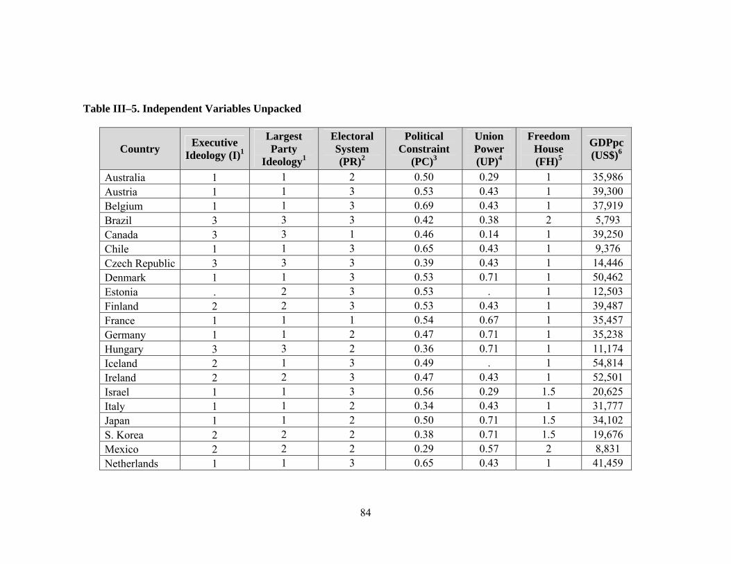
84

Table III–5. Independent Variables Unpacked

Country Executive

Ideology (I)1

Largest Party

Ideology1

Electoral System (PR)2

Political Constraint

(PC)3

Union Power (UP)4

Freedom House (FH)5

GDPpc (US$)6

Australia 1 1 2 0.50 0.29 1 35,986 Austria 1 1 3 0.53 0.43 1 39,300 Belgium 1 1 3 0.69 0.43 1 37,919 Brazil 3 3 3 0.42 0.38 2 5,793 Canada 3 3 1 0.46 0.14 1 39,250 Chile 1 1 3 0.65 0.43 1 9,376 Czech Republic 3 3 3 0.39 0.43 1 14,446 Denmark 1 1 3 0.53 0.71 1 50,462 Estonia . 2 3 0.53 . 1 12,503 Finland 2 2 3 0.53 0.43 1 39,487 France 1 1 1 0.54 0.67 1 35,457 Germany 1 1 2 0.47 0.71 1 35,238 Hungary 3 3 2 0.36 0.71 1 11,174 Iceland 2 1 3 0.49 . 1 54,814 Ireland 2 2 3 0.47 0.43 1 52,501 Israel 1 1 3 0.56 0.29 1.5 20,625 Italy 1 1 2 0.34 0.43 1 31,777 Japan 1 1 2 0.50 0.71 1.5 34,102 S. Korea 2 2 2 0.38 0.71 1.5 19,676 Mexico 2 2 2 0.29 0.57 2 8,831 Netherlands 1 1 3 0.65 0.43 1 41,459

85

Table III-5, continued

Country Executive

Ideology (I)1

Largest Party

Ideology1

Electoral System (PR)2

Political Constraint

(PC)3

Union Power (UP)4

Freedom House (FH)5

GDPpc (US$)6

New Zealand 1 1 2 0.45 . 1 26,173 Norway 3 3 3 0.52 0.71 1 72,960 Poland 1 1 3 0.56 0.71 1 8,958 Portugal 3 3 3 0.41 0.71 1 19,065 Slovak Republic . . 3 0.56 0.57 1 12,799 Slovenia 2 2 3 0.54 0.43 1 19,406 Spain 3 3 3 0.39 0.71 1 28,025 Sweden 3 3 3 0.51 0.62 1 43,949 Switzerland . . 3 0.42 0.33 1 54,140 Turkey . . 3 0.31 0.57 3 7,687 UK 3 3 1 0.40 . 1 40,481 United States 1 1 1 0.40 0.14 1 44,623

1 Right = 1, Centrist = 2, Left = 3; SOURCE: World Bank's Database of Political Institutions 2 Majoritarian=1, Mixed=2, Proportional Representation=3; SOURCE: World Bank's Database of Political Institutions 3 The index scores are derived from a simple spatial model and ranges from 0 to 1, with higher scores indicating more political constraint and thus less feasibility of policy change. “The index is composed from the following information: the number of independent branches of government with veto power over policy change, counting the executive and the presence of an effective lower and upper house in the legislature (more branches leading to more constraint); the extent of party alignment across branches of government, measured as the extent to which the same party or coalition of parties control each branch (decreasing the level of constraint); and the extent of preference heterogeneity within each legislative branch, measured as legislative fractionalization in the relevant house (increasing constraint for aligned executives, decreasing it for opposed executives)” (Teorell, et al. 2012, 108). Note that the coding reflects information as of January 1, 2006. SOURCE: QOG Database 4 Labor Union Power Index –“The average of the following seven dummy variables which equal one: (1) if employees have the right to unionize; (2) if employees have the right to collective bargaining; (3) if employees have the legal duty to bargain with unions; (4) if collective contracts are extended to third parties by law; (5) if the law allows closed shops; (6) if workers, or unions, or both have a right to appoint members to the Boards of Directors; and (7) if workers’ councils are mandated by law” (Teorell, et al. 2012, 29). SOURCE: QOG Database 5Most free = 1, least free = 7; SOURCE: Freedom House 6 SOURCE: OECD Country Data

86

What the 2006 data show in this chapter are the spending priorities of the

officials who held office that year – the EPI-A and EPI-M reflect the government’s

expenditures under their tenure. Electoral cycles are not directly addressed in the models

though the PC measure does address party conflict for the given year. For the countries

included in the analysis, 12 had legislative and 4 had executive elections in 2006

whereas 9 had legislative elections and 3 had executive elections in 2005. These

elections are listed in Appendix C. Although these events may have impacted 2006

spending priorities, the impact of the elections themselves are beyond the scope of this

analysis, rather this analysis addresses how party ideology and institutional constraints

impact the decisions political actors make once in office. Table III-7 presents the

regression analysis results.

Table III–6. Institutional and Ideological Impacts on Spending Decisions

Independent Variables EPI-A EPI-M

Executive Ideology -.05 (.03)* -.03 (.03) Electoral System -.24 (.07)** -.04 (.08) Union Power -.94 (.29)** -.04 (.35) Electoral System*Union Power .42 (.13)** .06 (.15) Freedom Index .12 (.07) -.07 (.09) Political Constraint .01 (.27) .06 (.32) GDPpc -.00 (.00)* .00 (.00)

Model p-value .03 .71 NOTES: N=26, Standard errors are in parentheses; Countries omitted due to lack of data are Estonia, Slovak Republic, Switzerland, and Turkey (no data for executive ideology) and Iceland, New Zealand, and the U.K. (no data for union power). *p<.10, ** p<.01

87

The EPI-A model has an overall p-value of .03 and an adjusted R2 of .36. As

mentioned above, Appendix B provides on overview of the expected sign directions

given the hypotheses begin tested. In summary, negative coefficients indicate a demand-

side policy orientation while positive coefficients indicate a supply-side policy

orientation. Of the significant independent variables the most remarkable is the type of

electoral system – having a government that is proportionally representative will likely

lead to more demand-side spending by as much as .25 on the EPI scale. Powerful unions

will also significantly push the EPI-A measure towards the demand-side of the scale.

The coefficient of the interaction of union power and electoral system cannot be directly

interpreted. Figure III-6 presents the marginal effect of powerful unions given a PR

system for electing officials and shows that as the electoral system moves from

majoritarian to mixed to proportionally representative, the power of unions has an

increasing impact on the balance of supply- and demand-side spending. This support for

Hypothesis 3.5 is significant in that it confirms the importance of unions and electoral

systems for budget allocations. This significance, however, is interactive and one

without the other will likely have a different outcome for beneficiaries.

88

Figure III–6. Marginal Effects of Union Power Conditional on the Electoral System

89

Section 3. 5. Conclusion

This chapter has shown that political institutions and the ideology of decision

makers have an impact on governments’ spending priorities between supply-side

(education) and demand-side (family and student benefits) policies. Namely, the type of

electoral system will have an impact on whether or not families, regardless of their

income level, will benefit from fiscally redistributive policies as much as or more than

schools will. Based on the analysis presented here, those countries that elect their

representatives via a PR system are going to be more redistributive and assure families a

higher level of benefits than governments that are elected via a majoritarian or mixed

system. Further, the electoral system will affect how much unions can influence

spending, and PR systems, as theory suggests, appear to give unions more leverage on

such decisions than majoritarian systems do. Left-leaning governments also play a

significant role regardless of how they are elected, and will push spending towards

family benefits, both means-tested and non-means-tested, over schools.

At the sub-national level, these institutional and political factors are also at play,

influencing state and local governments in their choice of which education policies they

pass and implement. Future research should look at the impact of these factors and their

effects on spending in greater detail. This dissertation does not completely ignore the

sub-national differences between countries, however. In Chapter IV the percent of

national, state, or local level fiscal and management decision-making related to schools

is incorporated into models analyzing how spending impacts student outcomes.

90

Another area for future research is the impact of international investments on

spending decisions. Most of the countries in this dataset are wealthy and only four,

Turkey, Mexico, Chile, and Brazil, have significant loans from the World Bank, other

countries, or other international monetary funding sources. Such outside monies are

known to impact policies. Chapter V in this dissertation provides a more details look via

a case study into how Mexico’s policies, funded in large part by the World Bank, have

had an impact on student outcomes.

The next chapter of this dissertation, Chapter IV, explores how spending between

supply- and demand-side policies impact student outcomes measured via a test of

cognitive skill. Such tests are irrelevant, though, if students are absent from school or if

students show up with an empty stomach, are sick, or do not live in a home where basic

needs are met. Research shows that when family benefits do not protect children from

poverty, they suffer cognitively and educationally (N. Ozawa 2004). All countries have

committed some level of their budgets to families regardless of the country’s level of

economic development. This chapter has shown that the variation in how much spending

goes to demand-side spending is greatly dependent on a country’s political system and

leadership ideology. The next chapter will show how these spending decisions have an

impact on countries’ human capital development.

91

CHAPTER IV

SPENDING AND HUMAN CAPITAL DEVELOPMENT

In the last chapter we saw how government institutions and leaders’ political

ideology at the national level have an impact on countries’ spending policies. In this

chapter we explore how these policies on education spending impact the development of

students’ marketable skills and knowledge, their human capital. As described in Chapter

II, the Education Policy Index (EPI) is designed to capture the balance of a country’s

supply-side spending, spending that targets schools and teachers, with the country’s

demand-side spending, spending that is geared to families and individual students. As I

have argued throughout this dissertation, both types of spending are necessary to help all

students succeed academically, but their impacts on students will be different.

Supply-side expenditures are expected to affect student learning and cognitive

development whereas demand-side spending is expected to increase or maintain

enrollment numbers – in some cases helping students who, due to financial

circumstances, might choose to forego their education altogether. While these two

outcomes are highly related (students can’t benefit from schools unless they are in

attendance), they need to be assessed differently. To test the success of school

investments (supply-side spending) across countries it is useful to look at student

performance on a common test of skills and knowledge such as the Programme for

92

International Student Assessment (PISA) exams, whereas to evaluate the success of

demand-side spending, school enrollment rates are the more useful measure.

Recall from Chapter II that the spending estimates used to create the Education

Policy Index for all types of demand-side spending (EPI-A), as well as the Education

Policy Index for means-tested demand-side spending (EPI-M), reflect expenditures from

all levels of government – not just spending from the federal level. While I was not able

to evaluate the subnational institutional and ideological influences on the spending

allocation decisions themselves, I can explore whether or not the source of funds impacts

the effectiveness of schools for purposes of human capital development, as well as

whether or not the level of government making education policy decisions impacts

student performance.24

The findings presented in this chapter indicate that demand-side expenditures in

the aggregate (means tested and non-means-tested) do have a positive impact on

enrollment rates and that this is mostly driven by the allocation of cash benefits and

benefits in kind to families and students (not financial aid). Measures of cognitive skill

and knowledge, results on the PISA exams, indicate that supply-side spending (spending

targeting schools and teachers) has a positive impact on student performance when

demand-side spending targets the most needy students. In analyses of institutional

decentralization and how management decision making affects human capital

development, local autonomy shows positive effects.

24 As discussed in Chapter III, evaluating subnational institutional and political differences between each country in the dataset is an area for further research. Ten of the countries in the dataset (Australia, Austria, Belgium, Brazil, Canada, Germany, Mexico, Spain, Switzerland, and the United States) are considered federal and would provide interesting case studies in later analyses.

93

In Section 4.1 the concept of human capital is introduced and discussed in terms

of enrollment rates and examination scores. The impact of EPI-A and EPI-M spending

on enrollment rates and examination scores are evaluated with regression models in

Section 4.2. The variation between countries’ national, regional, and local education

expenditures is explored in Section 4.3 along with differences in how schools within

countries are managed. Regression models from Section 4.2 are expanded to include

fiscal and management decentralization variables and the findings are presented.

Section 4.1. What Is Human Capital?

In the political science literature, when nations spend money on education

(schools and teachers), the expenditure is often considered a proxy for a country’s

investment in human capital (Kaufman and Segura-Ubiergo 2001, Avelino, et al. 2005,

Rudra 2005, Magnuson 2007). In the economics literature, human capital is understood

to be an individual’s accumulation of experience and personal attributes, as well as skills

and knowledge (Becker and Tomes 1986, Kan and Gershuny 2006). Education systems,

in addition to family and community influence, play a key role in the development of

human capital as it is the main venue for teaching skills and knowledge.

In Gary Becker's seminal 1964 book, Human Capital: A Theoretical and

Empirical Analysis with Special Reference to Education, he explains that “education and

training are the most important investments in human capital” (Becker 1962, 17). Becker

goes on to discuss credentialism as an alternative to human capital analysis in which

schooling is not the main contributor to one’s productivity, rather one’s level of

94

education is indicative of one’s abilities, persistence, and other characteristics (19).

These are not mutually exclusive conceptualizations, however. If one’s credentials are

indicative of how skilled and able one is to work, then educational attainment may serve

as a strong proxy for one’s level of human capital. Based on this logic, graduation or

even enrollment rates could reasonably be used to measure a country’s level of human

capital. Indeed, enrollment rates can be very useful for showing how much of country’s

population is participating in the education system that should, depending on the quality

of the school system, be enabling students to become employable members of the

society.

Secondary School Enrollment and Human Capital Development

Wealthier countries tend to have high primary and secondary school enrollment

rates. As shown in Figure IV-1, the countries in this dataset all have gross secondary

school enrollment rates of more than 75%. The secondary gross enrollment ratio

presented in Figure IV- is defined by the World Bank as the ratio of the total student

enrollment in secondary school, regardless of age, to the population of the age group that

officially should be enrolled in secondary school (World Development Indicators -

Aggregated Database 2009). The secondary gross enrollment rate is a useful measure for

assessing primary schools’ effectiveness at retaining students since students cannot be in

secondary school without first successfully completing the previous grades.

95

Figure IV–1. Secondary School Gross Enrollment Rates, 2009*

*Due to missing 2009 data, the enrollment estimates for Brazil and Canada are from 2008 SOURCE: World Bank, UNESCO Institute for Statistics, “World Development Indicators”

96

The majority of the countries on this list have gross secondary enrollment ratios

of around 100%, with only Turkey, Mexico, Chile, and the Slovak Republic with ratios

under 90%.25 Students are dropping out after middle school in these countries, if not

before, and the potential human capital gains from supply-side education spending are

consequentially lost on them. Countries that have a ratio over 100 appear to be dealing

with higher rates of grade repeaters, younger students entering grades, older students

returning to high school, or an immigrant population.

Policies that target the poor or that alleviate the costs of sending students to

school in the first place are advantageous for keeping the school-aged population in

classrooms. For the wealthy countries in the dataset used in this dissertation, demand-

side spending would be expected to maintain the high enrollment ratios these countries

report. For the countries that are struggling to keep their students in school, more

demand-side spending would be expected to help raise enrollment levels so that students

have the potential to develop the skills they will need to be economically competitive.26

25 The World Bank (2009) reports that the average enrollment ratio for the world’s countries in 2009 is 68% with a low of 12% in Niger. Less developed, highly illiterate countries offer interesting opportunities for exploring the impact demand-side spending can have on enrollment ratios over time, but detailed data are not currently available for these countries. In Chapter V of this dissertation, students from three rural Mexican schools provide evidence that demand-side spending can be influential for attendance decisions in places where enrollment is more of a challenge. 26 The percent change in gross secondary enrollment rates between 2006 and 2009 in the aggregate is less than 3% with some notable exceptions – Australia (-13%), Portugal (10%), and Turkey (-9%). The causes for enrollment changes are not always related to school expenditures. Australia and Portugal were still in the 100% or higher range so changes may be due to fewer older or younger students being enrolled. Turkey’s decline (from 85% to 78%) may be due to the worldwide recession but a country-specific analysis would be needed to discern the causes for this change. While demand-side spending may have played a role in moderating these changes the other factors that may be contributing to the change cannot be accounted for at this level of analysis. Accordingly, to avoid these exogenous factors, the 2009 gross enrollment rate is used.

97

Hypothesis 4.1: Demand-side spending should have a positive impact on countries’ student enrollment rates.

The sociology literature considers human capital to be one of three types of

attributes an individual may possess. In agreement with economists, sociologists

consider human capital to be the skills, knowledge, and educational attainment of

individuals that is considered of value for employment purposes. Social and cultural

capital, however, are also part of an individual’s assets. Sometimes they are integrated

and together form an individual’s capital, and in other studies one type of capital may

influence another (Kan and Gershuny 2006; Coleman 1988). For example, Coleman

(1988) argues that social capital, the connections people have with each other in a

society, can be understood to build human capital by its influence on keeping students in

school; his study focuses on high school. This approach is in line with economists in that

education attainment is a key determinant of human capital. The third type of personal

capital found in the sociology literature is cultural capital or “specific knowledge related

to the participation in, and enjoyment of, the various forms of consumption in the

society” (Kan and Gershuny 2006, 2). The literature indicates that these distinct types of

capital, cultural, social, and human, together are critical for understanding the

capabilities of individuals in a population.

Usually the economists’ approach is found in the political science literature.

Hershberg (1996), in his evaluation of the challenges facing America, defines human

capital as “the education, skill level, and problem-solving abilities that will enable an

individual to be a productive worker in the global economy of the twenty-first century”

98

(44). Given the similarities in how economists, sociologists, and political scientists

define “human capital,” for purposes of the dissertation, the definition of human capital

will be those skills and abilities of the working population that have economic value.27

What determines, however, which skills and abilities actually have a market

value? Moreover, how much of these skills and abilities can be attributable to what

happens in schools? Some students have the will, financial resources, and ability to

pursue general, higher-level degrees after secondary school while others choose a

vocational school or directly enter the labor market. The variation in skills and

occupations is vast. There is a literature that explores the connection between jobs and

skills and their relationship to education (Hartog 2000b, Hartog 2000a, Webbink and

Hartog 2004, Hartog and Vijverberg 2007). Webbink and Hartog (2004) go so far as to

claim that “expectations of earnings lies at the heart of the ‘human capital’ model. The

model states that students, in deciding on the amount of education, compare the

outcomes of the different options and choose the option with the highest return” (103).

This study found that in the Netherlands, students’ expectations (both at the individual

and group level) were realistic – and the underlying premise was that more education

would yield higher earnings. For some jobs, workers may be over or under educated and

the right mix of skills may be difficult to ascertain. Studies have looked at how to

resolve this via better curricula (Hartog and Vijverberg 2007).

27 Economic value in this definition implies an open-market value. Yet, academic knowledge, for example, does not necessarily have a general application that would make it marketable; however, the accumulation of knowledge is generally considered an important societal benefit. The employment of professors does indirectly imply a value for such activity so the value of knowledge would be included. The other concern with this definition is that it implies that monetary value is the only value that matters in a society. Cultural or social capital is also valuable, but unfortunately more difficult to measure since they are less tangible than employment.

99

The studies that look at human capital development over time can best identify

the causal mechanisms at work from school to family to community (Goldstein 2004).

While the most comprehensive (and expensive) studies would be able to trace causality

by evaluating, over time, the ways education or schools impact students’ human capital

development (and control for the social and cultural capital a student has access to

through their families and their communities), this is not always feasible or realistic;

following students throughout their academic and professional careers takes generations

of researchers and time. To begin to tap into what is going on in schools, however, I do

survey graduating middle school and high school students in Chapter V. In these

surveys, students are asked to articulate their academic and professional expectations

and assess how successful their school has been for them given their family and

economic circumstances. By looking to their assessment of how much school has helped

them develop their human capital, the impact of school and the resources they have

benefitted from can be understood at a more individual level. For cross-country analysis,

though, such an analysis is not feasible. Rather, at this level, an analysis of human

capital that uses a consistent and reliable multiple country assessment of cognitive skills

is more appropriate.

According to Hanushek and Woessmann (2011) there are many advantages to

this approach: “First, it captures variations in the knowledge and ability that schools

strive to produce and thus relates the putative outputs of schooling to subsequent

economic success; Second, by emphasizing total outcomes of education, it incorporates

skills from any source – families, schools and ability; Third, by allowing for differences

100

in performance among students with differing quality of schooling (but possibly the

same quantity of schooling), it opens the investigation of the importance of different

policies designed to affect the quality aspects of schools” (433-34).

The Programme for International Student Assessment and Human Capital Development

The Programme for International Student Assessment (PISA) is an assessment

that has been administered by the Organisation for Economic Co-operation and

Development (OECD) to 15-year-olds in over 40 countries every three years since 2000.

The PISA method is designed to measure a yield of student learning at age 15, so the

results should indicate how well students are able to apply their knowledge and skills in

mathematics, science, and reading to real-world problems. PISA features an “innovative

concept of ‘literacy’, which refers both to students’ capacity to apply knowledge and

skills in key subject areas and to their ability to analyze, reason and communicate

effectively as they pose, interpret and solve problems in a variety of situations” (OECD

2010e, 17). Given the learning tested by this assessment, and the contribution to learning

schools are expected to contribute to students’ development, supply-side spending,

spending going directly to teachers and schools, would be expected to positively

contribute to student performance.

Hypothesis 4.2: Supply-side spending will have a positive impact on PISA scores in all subject areas

101

The OECD has done a careful job to construct and translate their test items as

well as implement the exams along with surveys that were administered to principals,

students, and students’ families (OECD 2012d). For example, each item has two

different source languages (English and French) and each of these versions are translated

twice into the participating country’s language. A third person then reconciles the

translations. This double translation approach provides multiple opportunities to resolve

any semantic differences that would make the questions incomparable between countries

or misunderstood within the testing country.

While PISA resources are not limitless, test questions are developed with

considerable care and review. Input from participating countries is part of the item

development process and questions are extensively pilot-tested. In every country where

the PISA exam is implemented, there is a National Project Manager whose

responsibilities include coordinating exam question proposals and the review of all test

items, as well as test and survey implementation. To guarantee a representative sample

of a country’s schools and population demographics (the target population), the National

Project Managers establish a profile of the country’s education system and set the

appropriate criteria for the categories of schools. A minimum of 150 schools has to be

included in the implementation of the exam, and at least 35 students at each school are

randomly selected to avoid selection bias (each country has to have at least 4,500

students participating). The PISA Consortium that oversees the PISA exam

102

implementation makes the final school selections (not the National Project Managers) to

assure that random selections are made.28

Some have argued that even with the care taken to create the PISA exam, it is

still a test that only assesses how well students can take the PISA exam. “PISA gives a

relatively reliable assessment of ‘knowledge and skills for PISA’, that is, of how well

students exercise competence within the PISA focus areas in one—and only one—‘real

life’ situation, the PISA test situation” (Dohn 2007, 14). Standardized tests in general

have come under a great deal of criticism for decades.29 In the United States, Peter Sacks

wrote in his book Standardized Minds: The High Price of America’s Testing Culture and

What We Can Do to Change It (1999) that “standardized test scores tend to be highly

correlated with socioeconomic class … and standardized tests reward passive, superficial

learning, drive instruction in undesirable directions, and thwart meaningful educational

reform” (8). As discussed in Chapter II, the first criticism has validity – wealthier

students tend to do better on these assessments, including the PISA exam. However, this

does not negate the utility of using standardized assessment to gauge student learning.

By looking at how disadvantaged students perform given a set of criteria that can help

them do better and overcome obstacles, it is possible to innovate new reforms and

interventions, such as more demand-side expenditures or better supply-side targeting.

28 Japan is the only country whose National Project Manager oversaw the school selection because of “reasons of confidentiality” but there was careful oversight to assure that there was not bias in which schools were chosen (OECD 2012e, 71). 29 Universal tests of mental intelligence are sometimes traced back to the early 1900’s with the work of Frenchman Alfred Binet and his Binet-Simon scale (the precursor of the Stanford-Binet Intelligence Scale or what we call today the IQ test). In the over 100 years since these tests were created they have been highly criticized for their cultural and social biases, and many of these same critiques have been applied to modern standardized tests of knowledge.

103

This argument accepts that scoring well on tests such as the PISA exam is the desirable

end-goal for systems of education. Given the economic advantages higher scores yield, it

does seem that scoring better on the PISA assessment helps advance the development of

human capital as defined in this dissertation (the possession of marketable skills and

knowledge), making this objective a worthwhile one (Woessmann and Hanushek 2012).

Though PISA is in the end just a test, it is the leading tool to assess cross-

nationally how well students “can use their knowledge and skills to solve real world

problems rather than a test of whether they remember specific points of grammar or a

formula to solve a physics problem” (Sahlberg 2006, 282). As such PISA developers

claim that they avoid testing any one curriculum, rather, they argue it is a “forward-

looking” exam that asks students to show “what [they] can do with what they learn at

school” (OECD 2012e, 22).

In 2009, PISA was administered in 34 OECD countries and 41 partner countries

and economies. Table IV-1 lists the countries included in this dissertation along with

their 2009 PISA scores in reading, math and science. Unfortunately, PISA does not

distinguish between government-dependent private schools and regular private schools

so scores are only reported for private and public schools.30

30 The principals of all schools that participate in the PISA exam are surveyed and asked to identify if their school is considered a “private” or a “public” school. Sometimes a principal’s classification will put a government-dependent private school in the public school category, and sometimes it will go in the private school category. Based on these responses, and the scores of the students associated with these schools, a score for each school type is established. There is an “other” school category but these do not include government-dependent private schools and, if it is not zero, is a very marginal percent of the country’s tally. See Appendix A for these details.

104

Table IV–1. Country PISA Scores

2009 PISA Scores**

Country % Public % Government-

Dependent Private

% Public and Government-

Dependent Schools

% Private Schools*

PISA Scores Source

Reading Math Science

Netherlands 30% 70% 100% 0% All Schools 508 526 522 Belgium 44% 56% 100% 0% All Schools 506 515 507 Hungary 89% 11% 100% 0% All Schools 494 490 503 Austria 92% 8% 100% 0% All Schools 470 496 494 Slovakia 92% 8% 100% 0% All Schools 477 497 490 Sweden 92% 8% 100% 0% All Schools 497 494 495 Germany 93% 7% 100% 0% All Schools 497 513 520 Finland 93% 7% 100% 0% All Schools 536 541 554 Czech Republic

94% 6% 100% 0% All Schools 478 493 500

Norway 96% 4% 100% 0% All Schools 503 498 500 Israel 100% 0% 100% 0% All Schools 474 447 455 Australia 72% 28% 100% 0% All Schools 515 514 527 Denmark 87% 12% 100% 0% All Schools 495 503 499 Slovenia 98% 1% 100% 0% All Schools 483 501 512 Iceland 96% 4% 100% 0% All Schools 500 507 496 France 79% 21% 99% 1% All Schools 496 497 498 Korea 83% 16% 99% 1% All Schools 539 546 538 New Zealand

82% 14% 96% 4% All Schools 521 519 532

Spain 70% 25% 95% 5% All Schools 481 483 488

105

Table IV-I, continued 2009 PISA Scores**

Country % Public % Government-

Dependent Private

% Public and Government-

Dependent Schools

% Private Schools*

PISA Scores Source

Reading Math Science

U.K. 80% 15% 94% 6% All Schools 494 492 514 Chile 47% 47% 94% 6% All Schools 449 421 447 Ireland 99% 0% 99% 1% Public Schools 474 472 489 Turkey 98% 0% 98% 2% Public Schools 464 444 453 Estonia 98% 0% 98% 2% Public Schools 501 512 528 Switzerland 94% 2% 96% 4% Public Schools 500 534 516 Poland 96% 1% 96% 4% Public Schools 499 493 507 Italy 94% 0% 95% 5% Public Schools 489 486 492 Canada 94% 0% 94% 6% Public Schools 521 522 526 Portugal 87% 4% 91% 9% Public Schools 485 482 489 U.S.A. 91% 0% 91% 9% Public Schools 494 482 496 Japan 90% 0% 90% 10% Public Schools 522 531 542 Brazil 89% 0% 89% 11% Public Schools 398 373 393

Mexico 89% 0% 89% 11% Public Schools 420 414 411 NOTES: Table II-1 also shows the percentage of public, government-dependent private schools, and private schools for each country. PISA scores are only published based on private or public schools so there is no distinction made for government-dependent private schools. The percentages of school types data are repeated here to better explain why PISA scores are based on all schools (public and private) or only public schools in the analysis in Chapter IV. *Private schools exist in these countries even when 0% is listed but the number is negligible in the aggregate count of school types. **A weighted mean is used to determine a combined score for all types of schools within a country. (The scores of all private school students are averaged together and then multiplied by the percent of private schools that took the PISA exam in the country. The scores of all public school students are also averaged together and then multiplied by the percent of public schools that took the PISA exam in the country. These two numbers are added together to determine the country's PISA score). SOURCES: OECD Education Database, dataset: students enrolled by type of institutions and OECD Education Statistics Database (PISA Results 2009)

106

As discussed in Chapter II, about a third of the countries in this study have a

significant number of government-dependent private schools (over 10%) as reported by

the OECD. Accordingly, if only public school PISA scores are used, it would

misrepresent the skills gained by students who are benefitting from government funding.

To show how country PISA scores are determined, the percentage of public,

government-dependent private schools, and private schools for each country is listed

(this information is also included in Table II-1 in Chapter II).

The “PISA Score Source” column indicates if the scores used for purposes of

analysis in this chapter reflects the work of students from both private and public schools

or just public schools. If 100% of the schools in a country are public and government-

dependent private schools, then the total country scores are used (all scores from public

and private school students). If there are no government-dependent private schools in the

country, then the public school scores are used. The trickiest countries are those that

have a large number of government-dependent private schools and a fair number of

private schools. In Chile, for example, 47% of the schools are public and 47% of the

schools are government-dependent, leaving 6% of the population in private school. To

not include the government-dependent private school score altogether would ignore 47%

of the students who are benefitting from government funding. Accordingly, the overall

country score is used so the 6% of schools that are private have their students included in

107

the PISA score used for analysis. Appendix E lists the public and private school scores

for the students who completed the PISA exam.31

The difference in private and public school scores is reported in Table IV-2.

According to the OECD, “In PISA 2009, one school year’s progress corresponds to an

average of 39 score points on the PISA reading scale” (OECD 2012c, 95).32 In the

aggregate, the difference between public and private school students’ performance on

the PISA exams averages less than one year of schooling, yet in some cases there can be

as much as three years of difference in student performance. In Brazil, Slovenia, and

Turkey, public schools make up respectively 89%, 98%, and 98% of the schools, and

they have the largest disparities between public and private school student performance.

Based on the scores, there is a two to three-year gap between private school and public

school students’ abilities in these countries. Moreover, in these three cases as well as in

nearly all the countries in the analysis, private school students perform better on the

PISA exam. Much of the disparity has been attributed to the demographic differences in

students who attend public versus private schools – private school students are usually

more advantaged economically (OECD 2009a). In studies however, once the

socioeconomic status (SES) of students is controlled for, the gap in public and private

school students’ scores becomes unremarkable (OECD 2010e).

31 While PISA administrators try to pick a representative sample of school types to participate in the PISA exam, they cannot always exactly match the distribution. 32 The 39 points was calculated by subtracting the scores of students of the same age who were enrolled in at least two different grade levels.

108

Table IV–2. Gap in the PISA Score Between Public and Private Schools

Difference between Private and Public School Scores Country Reading Math Science Australia 45 38 41 Austria 32 12 18 Belgium 45 46 45 Brazil 118 112 112 Canada 45 60 41 Chile -26 -23 -22 Czech Republic 32 21 37 Denmark 17 14 20 Estonia 9 -10 1 Finland 6 -6 10 France a a A Germany 16 21 17 Hungary 15 19 14 Iceland a a A Ireland 35 25 31 Israel -4 -4 -4 Italy -41 -40 -37 Japan -8 -6 -9 Korea 16 12 9 Mexico 48 43 45 Netherlands -11 -8 -6 New Zealand 69 64 59 Norway -38 -44 -44 Poland 55 64 56 Portugal 31 32 27 Slovak Republic 24 17 16 Slovenia 80 97 89 Spain 36 31 31 Sweden 35 30 29 Switzerland 18 7 13 Turkey 82 127 92 UK 61 56 73 USA 71 61 68 Average 29 28 28

NOTES: a = not applicable (France did not categorize schools and Iceland did not report private school scores). The largest differences are in bold.

109

Despite the limitations of standardized tests discussed above, they do provide a

consistent cross-national measure with which to compare students (McBee 2002, Altinok

2008). In 2009, the central focus of the PISA exam was reading, though students were

also tested in mathematics and science. OECD analyses indicate that “across OECD

countries, overall performance in mathematics remained unchanged between 2003 and

2009, as did performance in science between 2006 and 2009” (OECD 2010f, 14).

Reading, however, did show mixed results – some countries improved while others did

not. In the aggregate, however, changes in scores between 2006 and 2009 were not

substantial enough for purposes of the analysis presented here and thus only the 2009

scores are used as the dependent variable in this study. In the next section, analyses

exploring how governments’ spending decisions impact enrollment rates and student

performance on the PISA tests of skill and cognition are presented.

Section 4.2. Human Capital and Education Investments

To begin the analysis I first want to test Hypothesis 4.1 that claims demand-side

spending will have a positive impact on enrollment rates. The gross enrollment rate of

each country is the outcome of interest (the dependent variable) and lower EPI scores,

scores that are closer to .5 and are more demand-oriented, would be expected to have a

larger impact on enrollment rates than EPI scores that are more supply-side oriented.

Thus, if demand-side spending is having the expected effect, if it is helping students get

to school and stay there, then as the EPI gets lower, enrollment rates should increase

making this relationship a negative one. While all of the countries in this dataset are

110

wealthy by international standards, five of them have a 2006 Gross Domestic Product

(GDP) per capita of less than $10,000 (Brazil, Chile, Mexico, Poland, and Turkey).33

Controlling for wealth with GDP per capita in the model is a way to account for the

societal advantages wealthier countries have for students that I am not capturing in the

EPI-A and EPI-M measures.34

Equations 4.1a and 4.2a look at the overall balance of demand- and supply-side

spending while Equations 4.1b and 4.2b split apart the EPI scores to isolate the demand-

side spending that is expected to influence the gross secondary enrollment rates.

gEnrollmentct = 0+ EPIAct-31 + GDPpcct-32 + eq. 4.1a

gEnrollmentct = 0+ PCashBenefitsA ct-31 + PBenefitsInKindA ct-32 + PFinancialAidA ct-33 + GDPpcct-34 +

eq. 4.1b

gEnrollmentct = 0+ EPIMct-31 + GDPpcct-32 +

eq. 4.2a

gEnrollmentct = 0+ PCashBenefitsM ct-31 + PBenefitsInKindM ct-32 + PFinancialAidM ct-33 + GDPpcct-34 +

eq. 4.2b

33 See Table II-5 in Chapter II for each country’s GDP per capita 34 Previous versions of this model used per pupil spending based on the overall EPI expenditures and enrollment rates as the control variable for wealth. Scatterplots reveal that this measure, though highly correlated with GDP per capita, misrepresents the advantages students coming from wealthier countries might have over students from less wealthy countries. For example, students in Slovenia appear to be benefitting more than students in Japan from education spending though Japanese students are considerably wealthier and have advantages the model would not otherwise be taking into account.

111

In Equations 4.1a through 4.2b, gEnrollmentct is the gross secondary enrollment

ratio for each country (c) at time (t), which is 2009.35 The EPIAct-3 in Equation 4.1a is

the 2006 Education Policy Index for which the supply-side spending includes all monies

allocated to public and government-dependent private schools in each country, and the

demand-side spending is both means-tested and non-means-tested. The EPIM ct-3 in

Equation 4.1b is the Education Policy Index for which the supply-side spending is all

monies allocated to schools and the demand-side spending includes only means-tested

benefits (see Chapter II for details on how the EPI-A and EPI-M variables are

constructed).

In Equations 4.1b and 4.2b, demand-side spending is split apart into its

components: cash benefits, benefits in kind, and student financial aid. Chapter II

explains how these categories are derived. The EPI-A categories for Equation 4.1b are

based on the percent of overall EPI-A spending (supply-side plus demand-side spending)

for each country (c) at time (t-3) or 2006 allocated to cash benefits (PCashBenefitsA ct-3),

benefits in kind (PBenefitsInKindA ct-3), and student financial aid (PFinancialAidA ct-3).

The EPI-M categories for Equation 4.2b are based on percent of overall EPI-M spending

(supply-side plus means-tested demand side spending) for each country (c) at time (t-3)

or 2006 allocated to cash benefits (PCashBenefitsM ct-3), benefits in kind

(PBenefitsInKindM ct-3), and student financial aid (PFinancialAidM ct-3).

35 Canada and Brazil reported gross enrollment ratios for 2008 rather than 2009. The gross enrollment ratio represents the overall enrollment for the entire country – public and all types of private schools. The source population data that counts the number of secondary-school aged citizens is not easily accessed making it difficult to determine the percent of this population subset that is going to public and government-dependent private schools. Regardless, the country’s gross enrollment rate should be sufficient for analysis as it is representative of the level of the education system’s hegemony.

112

Table IV–3. Spending and Gross Secondary Enrollment Rates

Equation 4.1a*** Equation 4.1b*** Equation 4.2a*** Equation 4.2b** Dependent Variable Gross Secondary

Enrollment Gross Secondary



Enrollment

EPI-A, 2006 -31.9** (14.9) Percent cash benefits-A 38.6** (17.7) Percent benefits in kind-A 37.0* (21.8) Percent financial aid-A 6.7 (26.7) GDP per capita, 2006 0.0002** (.0001) 0.0002* (.0001) 0.0004*** (.0001) 0.0004*** (.0001) EPI-M, 2006 -23.2 (17.6) Percent cash benefits-M 44.6 (42) Percent benefits in kind-M 27.9 (26.7) Percent financial aid-M 12.8 (23.3) Constant 118*** (10.3) 85.5*** (4.64) 113*** (15.5) 89.0*** (4.74) Observations 33 33 33 33 R-squared 0.372 0.397 0.283 0.298 NOTE: Standard errors in parentheses *** p<0.01, ** p<0.05, * p<0.1

113

Table IV-3 shows the results from Equations 4.1a through 4.2b. The outcomes

indicate that when countries spend more on supply-side expenditures (when the EPI-A

increases), enrollment estimates fall. This implies that if countries allocate more money

to demand-side expenditures (means and non-means-tested policies) relative to supply,

enrollment numbers increase. When the demand-side expenditures are only targeting the

most needy students (when they are means-tested), however, spending allocations,

regardless of what they are targeting, are not having as much of an impact on enrollment

numbers.

The results show that when the EPI-A categories are split apart into the demand-

side spending categories, the percent of cash benefits as well as family benefits in kind

has an impact on enrollment and this appears to be driving the significance of the EPI-A

in Equation 4.1a (when the overall EPI-A is the independent variable of interest). Based

on the adjusted R-square, we can say that nearly 40% of the variation in the enrollments

in Equation 4.1b can be explained by the cash benefits and family benefits in kind

expenditures.

There are no statistically significant findings for the EPI-M categories implying

that when benefits are generous to everyone, there is more general support for students

to go to school, and they go. Since GDP per capita is significant in all of the equations,

the enrollment numbers may also be a reflection of the fact that in wealthier countries

going to school is the norm and not going is the exception.

The point of school, however, is not just to show up. School is supposed to teach

students new knowledge and then how to apply that knowledge. As students work their

114

way from primary through to secondary school, their knowledge and skills should be

developing. By the time students are in secondary school, their cumulative knowledge

becomes the younger population’s human capital, and in this study this capital is

measured by student performance on the 2009 reading, math, and science PISA exams.

Hypothesis 4.2 asserts that supply-side spending in particular will positively impact

student performance on the PISA exam in all subject areas (reading, math, and science).

To begin to test this assertion, countries’ 2006 EPI-A and EPI-M scores, the balance of

supply- and demand-side spending, are the independent variables of interest. Since the

PISA exams are administered every three years, I applied a three-year lag to gauge the

success of policies implemented at the time of the last exam (2006) that may have an

impact on current (2009) scores. Students in secondary school in 2009 would have been

in school in 2006 so they would have had three years to benefit from advances in school

quality or from access incentives policies provide.

Unfortunately, the issue of school quality is not captured in the EPI – spending

on teachers does not mean that the teachers are effective at teaching, nor does spending

on materials or capital expenditures guarantee that anything meaningful is being

transferred to students. The PISA scores themselves, however, may be indicative of the

quality of the schools – if students are able to perform well on these tests they must be

prepared and the expectation is that the school contributed to this outcome in some

way.36 Gross enrollment ratios for each country are used as a control for the level of

36 As mentioned in Chapter III, teacher unions could be protecting teachers at the expense of quality learning, keeping bad teachers employed who are not helping students gain useful knowledge or skills. However, the “power of unions” variable used in Chapter III, when incorporated into models of human capital development, did not add any significance and proved to be an extraneous variable. Tapping into

115

student participation in the country’s school system (how popular going to school is for

the general population) and GDP per capita is used to control for the country’s wealth

and all of the advantages that wealth brings to human capital.

Human Capitalcts = 0+ EPIA ct-31 + GDPpcct-3 2 + gEnrollmentct3 +

eq. 4.3a

Human Capitalcts= 0+ EPIM ct-31 + GDPpcct-3 2 + gEnrollmentct3 +

eq. 4.3b

In Equations 4.3a and 4.3b, Human Capitalcts is the public and government-

dependent private school students’ scores on the PISA exams for each country (c) at

time (t), 2009, in subject (s) – reading, math, or science. The control variables are the

per-pupil spending and enrollment variables from Equations 4.1 and 4.2.

the impact of teacher unions on human capital development is an interesting question and future research should address this topic more intensely, however, it is currently outside the scope of this dissertation.

116

Table IV–4. Spending and Student Performance on the PISA Exam

Equation

4.3a** Equation

4.3a** Equation

4.3a** Equation 4.3b***

Equation 4.3b***

Equation 4.3b***

Dependent Variable

Reading Scores

Math Scores

Science Scores

Reading Scores

Math Scores

Science Scores

EPI-A, 2006 60.7 (38)

60.5 (49.9)

45 (47.7)

GDP per capita, 2006

0.0007** (.0003)

0.001** (.000)

0.001 (.000)

0.0004 (.0003)

0.0007* (.0003)

0.0004 (.0004)

Gross enrollment 2009

0.96* (.49)

0.91 (.65) 1.03 (.62)0.88* (.44)

0.86 (.58) 1.02*(.56)

EPI-M, 2006

105** (43.7)

118** (57.6)

97.9* (55.4)

Constant 331*** (64.6)

329*** (84.6)

342*** (80.9)

295***(62.5)

278*** (82.4)

293*** (79.3)

Observations 33 33 33 33 33 33

R-squared 0.32 0.30 0.25 0.37 0.34 0.29

NOTE: Standard errors in parentheses *** p<0.01, ** p<0.05, * p<0.1

The results in Table IV-4 indicate that when countries spend more on supply-side

policies, students have higher PISA scores – when the demand-side policies are means-

tested. When spending includes all types of demand-side spending (EPI-A), the model is

significant (p<.05) for each subject but GDP per capita or enrollment are the variables

that are explaining about 30% of the variation in students’ reading and math scores.

According to the OECD, “GDP per capita influences educational success, but this only

explains 6% of the differences in average student performance. The other 94% reflect

the potential for public policy to make a difference” (OECD 2010b, 3). This average

finding understates the impact of wealth in the countries included in this dataset.

117

When spending includes only means-tested demand-side spending (EPI-M), the

model is even more significant (p<.001) for reading and math outcomes, and supply-side

spending increases positively correlate with all subjects tested on the PISA exam. This is

remarkable since these EPI-M policies are targeting the most needy students and their

families and their inclusion in school is not lowering country PISA scores, rather they

seem to be positively influencing the overall scores. This could imply that the demand-

side spending has been incentivizing less advantaged students to go to school and to

prioritize their education, and that the supply-side spending may be effectively helping

students succeed academically. This could also imply that fewer disadvantaged students

are getting benefits and going to school in the first place so they are not having a

negative impact on PISA scores. In countries where enrollment rates are low this

concern warrants further investigation. However, in this dataset the enrollment rates are

high implying that most students are attending schools and participating in the system.

The impact on test scores based on the EPI-M balance of spending shows that by

increasing supply-side spending, students can gain three years of academic benefits in

math (118 points), and over two years of academic benefits in reading and science if a

year is equivalent to 39 points (See Table IV-4). A scatterplot of PISA 2009 Reading

scores to EPI-M (Figure IV-2) show that the spending balances of some countries such

as Turkey, Belgium, and S. Korea have comparable EPI-M scores but S. Korea has

significantly better scores on the PISA Reading exam.

118

Figure IV–2. EPI-M Scores to PISA Reading Scores

A scatterplot of PISA 2009 Reading scores to EPI-A (Figure IV-3) shows a

similar pattern – that countries with highly skewed supply-side spending do not

necessarily yield impressive test results.

119

Figure IV–3. EPI-A Scores to PISA Reading Scores

One underlying question is where is the supply-side spending going that is

having the impact on the scores? Equations 4.4a and 4.4b split apart the supply-side EPI-

A and EPI-M scores into their components to better understand which specific types of

supply-side spending are impacting student performance levels.

Human Capitalcts= 0+ PCompensationA ct-31 + PNonCompensationA ct-32 + PCapExpAct-33 + GDPpcct-3

2 + gEnrollmentct3 +

eq. 4.4a

Human Capitalcts= 0+ PCompensationM ct-31 + PNonCompensationMct-32 + PCapExpMct-33 + GDPpcct-3

2 + gEnrollmentct3 +

eq. 4.4b

120

In Equation 4.4a, the supply-side spending components are the percent of overall

EPI-A spending (supply plus demand-side expenditures) allocated to teacher

compensation (PCompensationA) for each country (c) at time t-3 or 2006, the percent of

overall EPI-A spending allocated to non-compensation benefits (PNonCompensationA),

and the percent of overall EPI-A spending allocated to capital expenditures

(PNonCompensationA). In Equation 4.4b, the supply-side subcategories are the same

compensation, non-compensation, and capital expenditures, but the percentages are

based on the EPI-M (supply plus means-tested demand-side spending). The results of

these equations are presented in Table IV-5.37

37 Chapter II explains how these components are calculated.

121

Table IV–5. Supply-Side Spending and Student Performance on the PISA Exam

Equation 4.4a**

Equation 4.4a*

Equation 4.4a*

Equation 4.4b***

Equation 4.4b***

Equation 4.4b***

Dependent Variable

Reading Scores

Math Scores Science Scores

Reading Scores


% Teacher compensation - A

43.1 (49.6) 30.0 (65.7) -2.05 (62.2)

% School Services - A

100 (102) 132 (135) 81.8 (128)

% Capital expenditures - A

403 (238) 356 (315) 444 (298)

GDP per capita 2006

0.0007* (0.0004)

0.001* (0.0005)

0.001 (0.0005)

0.0003 (0.0003)

0.0006 (0.0004)

0.0001 (0.0004)

Gross enrollment 2009

0.69 (0.58) 0.53 (0.76) 0.56 (0.72) 0.36 (0.47) 0.27 (0.63) 0.42 (0.60)

% Teacher compensation - M

108** (45.7) 119* (61.4) 87.7 (58.9)

% School Services– M

141* (73.2) 182* (98.4) 149 (94.4)

% Capital expenditures –M

462** (178) 451* (240) 483** (230)

Constant 343*** (77.0)

358*** (102) 387*** (96.5)

318*** (60.8) 309*** (81.8) 328*** (78.4)

Observations 291 291 291 291 291 291 R-squared 0.40 0.34 0.32 0.51 0.44 0.41

NOTE: Standard errors in parentheses 1 The omitted countries due to missing data are: Chile, Estonia, Hungary, and New Zealand (unlike their demand-side data, these countries do not disaggregate their supply-side data) *** p<0.01, ** p<0.05, * p<0.1

122

Since the EPI-A in Equation 4.3a did not yield any significant results we would

not expect any of the EPI-A supply-side spending categories to have an impact on

student outcomes. Accordingly, only GDP per capita has significance when Equation

4.4a is tested. Equation 4.4b uses means-tested demand-side policies only and the results

show that Capital Expenditures-M is the most significant supply-side spending category

across all subjects. Science appears to benefit the most from these expenditures though it

is not clear that laboratories or other facilities that might impact these scores are being

built with these funds. With more detailed data showing where the capital expenditures

are in fact going, it would be possible to better explain why the spending is having

positive impacts on each of the subject areas.

One question to consider from this analysis is what does means-tested demand-

side spending by itself tell us? To really assess the effectiveness of means-tested

demand-side spending, as opposed to all demand-side spending, I looked at the

proportion of demand-side spending that is means-tested.38 Figure IV-4 shows student

PISA reading scores (2006) and the proportion of demand-side spending that is means-

tested. Means-tested spending as a percent of all demand-side spending is not in fact

helping student scores, though, as we saw in Chapter I, it does help get students to

school. This finding indicates that attracting students to school who would otherwise not

be there is not, on its own, going to help student test scores. Rather, the experiences

students have at school are going to be more of the driving factors for improving test

38 This proportion is calculated by dividing the total means-tested demand-side spending by total demand-side spending.

123

scores. As discussed in Chapter I, school investments do positively correlate with how

resilient the poorest students are in each country that participated in the PISA exams.

Figure IV–4. Proportion of Means-Tested Demand-Side Spending and PISA Scores

Figure IV-5 shows that, when considering education spending to be money spent

on schools and means-tested demand-side policies, no country spends more than 15% of

their education expenditures on infrastructure (capital expenditures) and the Netherlands,

Norway, and South Korea are leading the countries in the dataset by spending over 10%

on these types of expenses. The level of investment by these countries raises questions

around what is being purchased with this money that is so significantly impacting

student outcomes.

124

Figure IV–5. Percent Capital Expenditures - M and 2009 Science PISA Scores

The percent of teacher compensation based on the EPI-M expenditures is another area of

spending that benefits student scores in reading and math. This result confirms the

importance of teachers, especially when the most disadvantaged students are benefitting

from policies that are encouraging them to come to school. Though it is not possible to

determine if this spending is for more teachers or paying teachers more (or something

else) it does encourage a closer look at how teachers are being compensated and which

practices are producing this effect. Non-compensation spending is also significantly

correlated with higher PISA scores in reading and math. As the demand-side spending

becomes more targeted, students appear to be benefitting more, indicating that helping

125

the most disadvantaged families does have an impact on education spending

effectiveness overall.

Section 4.3. Expenditure Sources and Decision Making In Education Spending – Do

They Impact Human Capital?

Research has shown that institutional elements such as decentralization and

school autonomy incentivize schools and teachers, and this leads to higher student

achievement (Woessmann and Hanushek 2012, 432). To this end, perhaps where the

money is coming from – which level of government is funding education – and where

school management decisions are being made will make a difference for student

performance on tests of knowledge and skill.

The funding sources for the supply-side spending portion of the EPI-A are highly

variable across countries. The UNESCO-OECD-Eurostat (UOE) data compiled from

reporting countries’ ministries of education or national statistical offices are shown in

Figure IV-6 and includes monies transferred between levels of government.

Figure IV–6

NOTE: SwedeSOURCE: OE

0%

10%

20%

30%

40%

50%

60%

70%

80%

90%

100%

6. Percentage o

en did not provide aCD Education Dat

of Supply-Side

any expenditure dataset: Expenditure b

Expenditures f

ta by funding source (

Centra

126

from Each Lev

(OECD 2012a)

al Regional

vel of Governm

Local

ent, 2006

127

Some countries, like New Zealand, Portugal, and Italy, rely primarily on their

central government for their education monies. Countries like Australia, Belgium and

Mexico, however, rely more heavily on regional governments (though the central

government may still be directing much of the budget allocations, as in Mexico) and

finally, countries such as Finland, Poland, and the United Kingdom mainly rely on local

government revenues.39

To see how much the level of government expenditures impacts student

performance on the PISA exams, the percent of local government spending was added as

an independent variable to Equations 4.3a and 4.3b. These regression models (not

shown) were significant but the local spending variable was not significant, and the

results from the earlier regression analysis held even with fewer degrees of freedom.

This outcome reconfirms that supply-side spending relative to means-tested demand-side

spending significantly impact student test scores regardless of the source of the money.40

Does Decision-making Decentralization Matter for Human Capital Development?

Finland, a country with the highest science 2009 PISA score in the dataset, and

the second highest math and reading scores after South Korea, has had its students place

in the top five on the PISA exams in all subjects since the test was first implemented in

2000. Finland has a strong commitment to equitable education opportunities and its EPI-

39 This dissertation does not address taxation issues associated with education and social expenditures, nor does it address how much private investment goes into public and government-dependent private schools. While these factors are germane to the discussion, only actual government expenditures and their institutional source is under analysis in this dissertation. 40 The percent of central spending expenditures was also used as an independent variable and the scenarios were consistent – where supply-side monies were coming from was insignificant whereas the amount of supply-side spending was significant, especially when the EPI-M measure was applied.

128

A score of .56 reflects its welfare state status. Fairly balanced between supply- and

demand-side spending, Finland spends 55% of its budget on schools and 45% of its

budget on individual students and families. Most of Finland’s spending, 33%, goes to

personnel expenditures and its next biggest expenses are cash benefits (23%) and then

benefits in kind (20%). Only 5% of Finland’s supply-side spending goes towards capital

expenditures (see Table II-2 in Chapter II for the EPI-A category details).

Finland is committed to providing students with access to its schools and has

done a good job providing quality schools once all students are there. Primarily locally

funded, 93% of Finland’s schools are public and the remaining 7% are government-

dependent private schools (the private schools were so heavily subsidized that they

eventually became part of the public school system). These schools, called peruskoulu,

are comprehensive schools for students in grades 1 to 9. They provide a common

curriculum, health and dental services, hot meals, and mental health services to all

students regardless of need. There is also ongoing assessment of students that are used

formatively – to mark where teachers need to target lessons. Once students complete this

level of education they go onto high schools that select students based on their academic

performance.

With its success, the Finnish school system has become a model for countries

around the world and the autonomy Finland gives its schools has been of great interest to

those advocating decentralized school management. In fact, there has been a substantial

move to empower schools through what is called Schools-Based Management (SBM)

because “most countries whose students perform well in international student

129

achievement tests give their local authorities and schools substantial autonomy over

adapting and implementing educational content, allocating and managing resources, or

both” (Barrera-Osorio, et al. 2009, 6). Research based on the PISA exams and associated

surveys suggest that budget autonomy for schools has a negative impact on student

success but management decisions, such as the hiring of teachers, can have a positive

impact on student cognitive skills (Woessmann, et al. 2009).

To discern how much autonomy schools enjoy over their resources, curriculum,

and personnel, the OECD Education group has administered a “Survey on Decision-

Making” every four years since 2003. A panel of national experts on lower secondary

education from each participating country is created to respond to these surveys and the

panels are designed to have representation from each of the government decision-making

levels (the central government, middle governments, and individual schools). The group

is supposed to form a consensus on responses to each question when they are completing

the survey (OECD 2012c, 4-6).

The surveys are broken up into four categories or indicators: organization of

instruction, planning and structures, personnel management, and resource management.

Organization of instruction questions ask panels to indicate which level of government

makes decisions related to curricula, pedagogy, tracking (if applicable), and essentially

anything related to teaching and learning decisions in the classroom. Planning and

structures questions include the overall design of programs of study, credentialing, and

school closures or openings. Personnel management includes hiring, firing, and salary

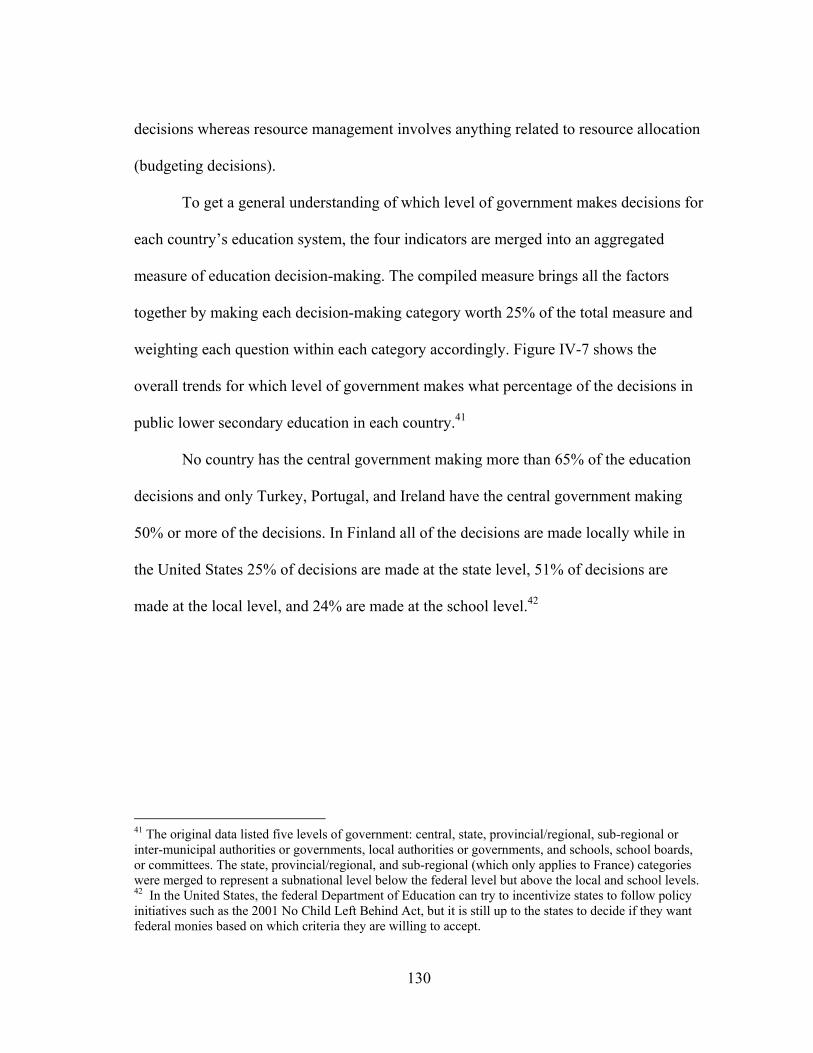
130

decisions whereas resource management involves anything related to resource allocation

(budgeting decisions).

To get a general understanding of which level of government makes decisions for

each country’s education system, the four indicators are merged into an aggregated

measure of education decision-making. The compiled measure brings all the factors

together by making each decision-making category worth 25% of the total measure and

weighting each question within each category accordingly. Figure IV-7 shows the

overall trends for which level of government makes what percentage of the decisions in

public lower secondary education in each country.41

No country has the central government making more than 65% of the education

decisions and only Turkey, Portugal, and Ireland have the central government making

50% or more of the decisions. In Finland all of the decisions are made locally while in

the United States 25% of decisions are made at the state level, 51% of decisions are

made at the local level, and 24% are made at the school level.42

41 The original data listed five levels of government: central, state, provincial/regional, sub-regional or inter-municipal authorities or governments, local authorities or governments, and schools, school boards, or committees. The state, provincial/regional, and sub-regional (which only applies to France) categories were merged to represent a subnational level below the federal level but above the local and school levels. 42 In the United States, the federal Department of Education can try to incentivize states to follow policy initiatives such as the 2001 No Child Left Behind Act, but it is still up to the states to decide if they want federal monies based on which criteria they are willing to accept.

Figure IV–7

NOTE: The deand the UnitedSOURCE: OEsecondary educ

0%

10%

20%

30%

40%

50%

60%

70%

80%

90%

100%

7. Percentage o

ecision-making datad States) are from 2CD 2012d (Educatcation (2003, 2007

of Overall Educ

a for eleven countr2011 and the other ction at a glance, Ta

7, 2011)

Central

cation Decision

ries (Belgium, Canacountries rely on 20

able D6.5). Trends i

l State/Provin

131

n-Making from

ada, Chile, Finland007 data. Brazil dain the percentage o

ncial/Regional

Each Level of

d, Ireland, Israel, Poata are unavailable.of decisions taken a

Local School

f Government, 2

oland, Slovak Repu. at each level of gov

l

2007/2011

ublic, Switzerland,

vernment in public

Turkey,

lower

132

To begin to see if Finland’s successful model of local school decision-making

holds across the countries in this dataset, the original equations of human capital

development (Equations 4.3a and 4.3b) are augmented with the percent of decisions

made at the local level.

Human Capitalcts = 0+ EPIA ct-31 + GDPpcct-3 2 + gEnrollmentct3 + LocalDMc4 +

eq. 4.5a

Human Capitalcts= 0+ EPIM ct-31 + GDPpcct-3 2 + gEnrollmentct3 + LocalDMc4 +

eq. 4.5b

The variable for the percent of education decision-making that happens in each country

(c) at the local level is “LocalDM”.43 The other variables are the same as in the earlier

analysis and the results from the regression are listed in Table IV-6. For students’ PISA

reading scores, the percent of local decision-making has a significant impact whether

there is means-tested demand-side spending or not in reading and science (only

significant for EPI-A) but not math. Further analysis into each of the four categories of

spending (resource and personnel management, the organization of instruction, or

planning and structures) at the local level does not yield any results at any level of

decision-making (models not shown). The only variable that has any significance in

these models is the gross secondary enrollment rate control variable that accounts for the

general level of student participation in the education system.

43 For most countries in the dataset, the decision-making estimates come from 2007. However, as indicated at the bottom of Figure 4.6, some countries did not respond to the survey questions until 2011. Although the level of decision-making might have shifted between 2007 and 2011, any shifts would be expected to be small or incremental.

133

Table IV–6. Local Decision Making and Student Performance on the PISA Exam

Equation 4.5a***

Equation 4.5a*

Equation 4.5a**

Equation 4.5b**

Equation 4.5b**

Equation 4.5b**

Dependent Variable Reading Scores Math Scores

Science Scores

Reading Scores


EPI-A, 2006 39.8 (30.9) 32.9 (43.4) 19.9 (40.1)

GDP per capita, 2006 0.0002 (.0003) 0.0004 (.0004)

0.0001 (.0004)

0.0001 (.0003)

0.0004 (.0004)

.0000 (.0004)

Gross enrollment 2009 1.22*** (.41) 1.10* (.57) 1.32** (.53) 1.05** (.39) 0.97* (.54) 1.22** (.5) Percent decision making – local 34.4** (16.4) 22 (23) 38.6* (21.2) 32.4* (16.9) 20.2 (23.4) 38.3* (21.6) EPI-M, 2006 29 (43.5) 25.7 (60.2) 2.14 (55.5)

Constant 328***(53.2) 341***(74.6) 341*** (69.1) 349*** (57.7) 357*** (79.9) 364*** (73.7) Observations 32 32 32 32 32 32 R-squared 0.39 0.27 0.31 0.36 0.26 0.3 NOTES: Standard errors in parentheses, Brazil data do not exist *** p<0.01, ** p<0.05, * p<0.1

134

One explanation for these null findings is that there may be an interaction

between resource and personnel management decisions at the local level but regression

analyses exploring this possibility did not reveal that the variables of interest had any

significance. The underlying decisions themselves that are not part of this analysis may

better explain the impact of local decision making. Theory and previous research would

suggest that there is more motivation for local decision makers when they have more

autonomy coupled with more public accountability via posted student test scores or a

final exit exam for students (Woessmann, et al. 2009). Future research should further

explore these decisions and their impacts.

Given the significance of local education decision-making, is there a negative

impact when governments centralize their education systems? Equations 4.6a and 4.6b

explore the same human capital development equations but instead of adding the percent

of local decision making, the percent of central education policy decision-making is

used.

Human Capitalcts = 0+ EPIA ct-31 + GDPpcct-32 + gEnrollmentct3 + CentralDMct4 +

eq. 4.6a

Human Capitalcts= 0+ EPIM ct-31 + GDPpcct-32 + gEnrollmentct3 + CentralDMct4 +

eq. 4.6b

The results are listed in Table IV-7 and show a significant and negative

correlation across all subject areas between central decision-making and student

performance for both the EPI-A and EPI-M measures of spending.

135

Table IV–7. Centralization and Student Performance on the PISA Exam

Equation 4.6a***

Equation 4.6a**

Equation 4.6a***

Equation 4.6b**

Equation 4.6b**

Equation 4.6b**

Dependent Variable

Reading Scores

Math Scores

Science Scores

Reading Scores

Math Scores

Science Scores

EPI-A, 2006 37.6 30.9 17.1 (30.4) (40.3) (38.0) GDP per capita, 2006

0.00027 0.00045 0.00016 0.00019 0.00039 0.00013

(0.0003) (0.0003) (0.0003) (0.0003) (0.0003) (0.0003) Gross enrollment 2009

0.91** 0.85 0.96* 0.76* 0.70 0.84*

(0.39) (0.52) (0.49) (0.38) (0.49) (0.46) Percent decision making – central

-46.8** -61.5** -65.4** -44.9** -61.2** -67.0**

(20.1) (26.7) (25.1) (21.1) (27.6) (25.8) EPI-M, 2006 20.6 5.59 -14.0 (43.5) (56.9) (53.2) Constant 374*** 385*** 398*** 399*** 417*** 435*** (51.8) (68.6) (64.7) (59.8) (78.3) (73.2) Observations 32 32 32 32 32 32 R-squared 0.41 0.37 0.38 0.38 0.36 0.38 NOTES: Standard errors in parentheses *** p<0.01, ** p<0.05, * p<0.1

Essentially as more decisions are centralized, students are benefitting less from

their school experience and they are not learning as much as they would from schools

that are operating with local oversight.44

44 The regressions were run with each level of government and only the local and central levels had any impact on student scores. State and regional, as well as school levels, produced insignificant results.

136


The EPI measures provide some insight into how spending is impacting student

enrollment rates and assessment scores which are in turn indicative of students’ level of

social and human capital development. Demand-side expenditures in the aggregate

(means tested and non-means-tested expenditures that target families and students) do

have a positive impact on enrollment rates. Further analysis of the demand-side spending

shows that cash benefits and benefits in kind to families and students, rather than

financial aid, are having the largest effects on gross secondary school enrollment. When

countries target their demand-side spending to the most disadvantaged families and

students and when they invest proportionally more in their schools, their students get

better results on PISA exams. Though it is not possible to conclude that this supply-side

spending provides students with top quality schools and the resources they need to

succeed, it is implied.

As current research on what makes schools successful suggests, local decision

making on the management of schools has a positive effect on student performance on

the PISA exams. PISA research has revealed two things about autonomy: 1) Students

who attend schools that can decide what is taught and how students are assessed do

better on PISA exams and 2) in countries where accountability measures are not publicly

available, schools that have more autonomy have students who do worse on PISA exams

(OECD 2010e). The next step for assessing the success of local management of schools

then, would be to explore different models of student assessment and how this impacts

student outcomes but this is beyond the scope of this dissertation.

137

If a country is truly committed to improving its human capital it needs to spend

money to help its less advantaged students get to, and stay in, school. Simultaneously,

education spending needs to maintain and improve the quality of its public schools so

that all students, once they get through the front doors, have the resources they need to

learn. Where the money actually comes from does not appear to make a difference for

human capital development – what matters is how the money is allocated.

To further complicate research into school systems, it is clear that there are

multiple pathways to student success. As the variation in EPI-A and EPI-M scores

reveal, countries with very different spending priorities are each able to successfully

educate students who can achieve high marks on the PISA exam. The three highest

scoring countries in reading, South Korea, Finland, and Japan, have EPI-M scores of .97,

.95, and .89 respectively, and these same countries score at the top for science as well as

math. These differing EPI-M scores, while not as variable as these same countries’ EPI-

A scores, show that successful countries are not doing things exactly the same way.

Capital expenditures, the most significant supply-side spending category in the analysis

when only means-tested demand-side spending is considered, is similar between the

countries. Both Japan and Finland spend about 9% of their resources on capital

expenditures while South Korea spends around 10% when EPI-M supply and demand-

side spending is considered together. How these funds are being allocated would show

how similar (or different) these expenditures are and why this spending in particular

matters for students’ level of achieved human capital. In the next chapter, human capital

development will be explored at the student level in three rural Mexican schools. Means-

138

tested demand-side benefits are received by most of the students in the case studies and

the impact of that spending is explored in more detail.

139

CHAPTER V

THE IMPACT OF DEMAND-SIDE EDUCATION SPENDING IN RURAL

MEXICO: THREE CASE STUDIES

This dissertation introduced the Education Policy Index (EPI) in Chapter II and

discussed why countries have the EPI scores they do in Chapter III. In Chapter IV, how

the EPI impacts student success academically was evaluated. Thus far, students’ gross

secondary enrollment rates and their scores on the Program for International Student

Assessment (PISA) exam have served as a proxy for human capital or students’

marketable knowledge and skills. This chapter goes beyond these measures and

discusses human capital indirectly by asking graduating students at two middle schools

and one high school in rural Mexico about their social capital: their grades, school

experience, and expectations of their future. Surveys administered at these three schools

in the summer of 2012 asked graduating middle school and high school students to

discuss their attitude towards school as well as their educational and professional goals –

indicators that if achieved could forecast a country’s economic growth. Most of these

students are extremely poor and 55% to 80% of them benefit from an established means-

tested demand-side spending program called Oportunidades.

Since supply-side spending at the school level is constant (students in the same

classroom experience the same teachers and infrastructure), the differences between

students within schools stems from their academic abilities, inspirations, and socio-

140

economic backgrounds. Across schools, however, it is possible to evaluate some of the

supply-side differences and how these may impact students’ attitudes towards school,

academic achievement, and their potential careers. Principal interviews and surveys,

school test scores, along with some school-level budget data, provide insight into the

quality of the education schools provide. This analysis shows that middle school and

high school students, and girls especially, who benefit from the demand-side policy

evaluated in this research, Oportunidades, are at least as likely as their wealthier

classmates to have high academic aspirations. It is more difficult to determine the

difference between students when it comes to evaluating their professional expectations,

however. Oportunidades appears to bring students of all financial circumstances together

and creates a more even starting point so that nearly all students, regardless of their

circumstances, can imagine a career that will provide a comfortable standard of living.

Nearly all students, regardless of their background, recognize the importance of school

for their future.

Section 5.1 introduces Oportunidades, Mexico’s demand-side policy, Section

5.2 explains the school system in Mexico and Section 5.3 discusses how Oportunidades

impacts Mexico’s school system. Section 5.4 presents the analysis of how students who

benefit from Oportunidades are impacted by their school attendance, Section 5.5

discusses the challenges schools face based on principal interviews, Section 5.6 presents

student opinions, and Section 5.7 presents analyses of the student survey data.

141

Section 5.1. OPORTUNIDADES: Mexico’s Leading Demand-Side Policy

Started in the late 1990’s and known as the Program for Education, Health, and

Food or PROGRESA (Programa de Educación, Salud y Alimentación) until 2001,

Opportunities or Oportunidades is Mexico’s largest anti-poverty program. Funded in

part by the Mexican Government, in part by the World Bank, and in part by the Inter-

American Development Bank (IADB), Oportunidades benefitted approximately 28

million people in 2011 at a cost of US$4.8 billion (Braine 2006; INEGI 2010; ECLAC

2011).45 It is a conditional cash transfer program (CCT) that pays qualifying poor

households on average US$35-40 a month if they meet a set of educational, health, and

nutritional requirements including regular school attendance and medical appointments

(Parker 2003; Fernald, et al. 2008; Oportunidades 2008; Behrman, et al. 2012). The

program is currently run by Mexico’s Ministry of Social Development or SEDESOL

(Secretaría de Desarrollo Social) and is implemented by the National Department for

the Oportunidades Human Development Program; since January 2012 funding for

Oportunidades comes through the Ministry of Public Education (SEP) budget (World

Bank 2010).

When the CCT program was first implemented as PROGRESA in rural areas in

1997, there was some evidence that beneficiaries were receiving the cash transfers as an

act of patronage, though most poor rural families were in fact benefitting (Yuriko 2007;

Yanes 2011). To reach the poorest populations, the federal government first targeted

impoverished municipalities based on 1995 census data, then identified the poorest

45 This is about 25% of Mexico’s 112,336,538 people and represents 5.8 million families.

142

homes, and then went to those homes to verify the conditions and who lived in the

households (Behrman and Skoufias 2006; Gertler, et al. 2012). Because the households

continue to be geographically targeted via a proxy means test (i.e., indicators that

correlate with poverty levels are used to determine family eligibility), the cash transfers

in theory cannot be withheld or distributed with discretion (Diaz-Cayeros, et al. 2012;

Cecchini and Madariaga 2011).

Moreover, even before Vicente Fox became president of Mexico in 2000 and

changed the program’s name to Oportunidades, certain mechanisms were put in to place

to limit patronage through the program. For example, there are public information

campaigns to directly communicate with beneficiaries, household eligibility reviews do

not take place around election time, and the central government keeps local involvement

over beneficiary decisions minimal – one exception being that it is the schools and

medical professionals who confirm that families are meeting policy requirements (Parker

2003; Levy 2006; Jara 2008; Diaz-Cayeros, et al. 2012). Even the skeptics, though,

agree that most of the eligible poor are being identified and benefitting from the program

(Jara 2008; Cecchini and Madariaga 2011; Gómez Hermosillo 2011).

As of 2010, according to the World Bank, 51.3% of the Mexican population lives

at the national poverty line and, in rural areas, this is as high as 60.8% (World Bank

2012a).46 Oportunidades claims that these high levels are due to the 2008 global

economic recession, and that these poverty estimates would be even worse without its

46 The World Bank defines the poverty rate as the “percentage of the population living below the national poverty line. National estimates are based on population-weighted subgroup estimates from household surveys” http://data.worldbank.org/indicator/SI.POV.NAHC/countries/MX?display=graph.

143

conditional cash transfers (SEDESOL 2010). Independent analyses show that

Oportunidades helps to reduce the depth of poverty of participants and also show that

the long-term living standards of poor rural families increases when they invest their

cash in productive assets such as chickens or other animals (Behrman and Skoufias

2006; Gertler, et al. 2012 ). In terms of overall inequality, the program does appear to

have an impact on Mexico’s Gini coefficient and one estimate claims that the program

has contributed to a reduction of 2.7 points (Cecchini and Madariaga 2011, 119).

Eligibility to receive Oportunidades cash payments for students starts in the third

grade and goes through high school, and the amount increases every year for both boys

and girls (See Appendix F for the 2010 payout to families).47 By some measures,

participating families’ income can increase by 10% per capita and for the poorest, cash

transfers may increase per capita income by as much as 50% (Fiszbein and Schady 2009,

109-10; Cecchini and Madariaga 2011, 117-18). To incentivize girls to continue with

their education, they are paid up to 13% more than boys starting in middle school when

they usually drop out (SEDESOL 2010). In addition to these scholarships, students

receive money for school supplies every 6 months. Further, students who complete high

school before turning 22 will receive a Youth With Opportunities (Jóvenes con

Oportunidades) bonus of nearly US$300 if they open their own savings account at a

bank (SEDESOL 2010; Gómez Hermosillo 2011).

47 In third grade students are usually between 8 and 9-years-old, about the age they would often be taken out of school to work. The program has changed since its inception and now includes funding for children under the age of 9 as well as the elderly. To qualify, families must meet means-tested poverty requirements.

144

Studies show that students whose families benefit from Oportunidades are more

likely than other poor students to stay in school between elementary and middle school

(Schultz 2004). “Research reveals that PROGRESA has had the largest impact on

children who enter secondary school and represents a percentage increase of enrollment

of more than 20% for girls and 10% for boys” (Skoufias 2005, xii). Since 2001 high

school students have been included in Oportunidades and longitudinal analyses reveal

that high school enrollment numbers have increased (Behrman, et al. 2011, 116). In

Chapter IV the receipt of demand-side benefits was shown to have a positive impact on

enrollment levels and the evidence here confirms this assertion.

Given how large the program has grown, Oportunidades now serves most of the

poorest students in Mexican communities. Based on the research on Oportunidades’

impact on enrollment rates and the findings in Chapter IV, students who benefit from the

means-tested program should be at least as likely as their peers who do not need to

receive the benefit to go onto high school.48

Hypothesis 5.1: Middle school students who benefit from Oportunidades are at least as likely as their peers who do not benefit from Oportunidades to go on to high school

Since females get more financial aid from Oportunidades then their male

counterparts for going to high school, and by some accounts are enrolling as much as or

48 All hypotheses consider students who receive benefits to be at least as or even more ambitious than their classmates academically and professionally. The cash incentive should be helping them reach a baseline of interest in their future and they may be more ambitious than their peers since they have more to overcome to attain the standard of living they see their peers enjoy.

145

more than males, they would be expected to want to go to high school at least as much as

male beneficiaries (Parker 2003). Additionally, since students who benefit from

Oportunidades are incentivized to stay in school, their academic aspirations would be

expected to exceed their parents’ level of education that usually did not continue past

primary school.

Hypothesis 5.2: Female middle school students who benefit from Oportunidades are at least as likely as their male counterparts to go on to high school

Hypothesis 5.3: Middle school students who benefit from Oportunidades are at least as likely as their peers who do not benefit from Oportunidades to want to attain a higher level of education than their parents

Behrman, Parker and Todd (2011) also show that students benefitting from

Oportunidades seek work and males in particular find nonagricultural jobs, implying a

shift away from the rural environment in which they are raised. Female students, whose

mothers receive the cash benefits of Oportunidades, see their mothers become

empowered as they take control over a part of the family finances and become more

informed about the health care of the family (Behrman and Skoufias 2006). Accordingly,

high school students’ career expectations should be higher than their parents’ current

career choices. In addition, like middle school students, high school students who are

benefitting from education incentives would be expected to want to attain a higher level

of education than their parents so long as education opportunities are available.

146

Hypothesis 5.4: High school students who benefit from Oportunidades are at least as likely as their peers who do not benefit from Oportunidades to want to attain a higher level of education than their parents Hypothesis 5.5: Male high school students who benefit from Oportunidades will be at least as likely as their peers who do not benefit from Oportunidades to seek nonagricultural jobs

With respect to how well Oportunidades students do in school once they

are there, beneficiaries can keep their funding so long as they do not fail a grade

more than once. On the other end of the success scale, though, while students are

staying in school longer, there is no indication that they are doing better on tests

of skills and knowledge (Behrman, et al. 2005). This raises questions around the

quality of the schools students are being incentivized to attend – are they able to

handle the increased enrollment numbers and what are they offerings students

once they get through the front door?

Section 5.2. Mexico’s School System: Supply-Side Policies In Action

The Mexican school system is mandatory for students until they have completed

at least a lower secondary level of education (the equivalent of kindergarten through the

ninth grade in the United States). If students want more schooling, they can go on to

upper secondary schools or high schools, and then tertiary schools or institutions of

higher learning (see Appendix 5B for an outline of Mexico’s public school system).

Approximately 90% of Mexico’s students attend public schools that are largely run by

147

the federal Ministry of Public Education (SEP) in spite of attempts in the 1990’s to

decentralize the system.

The National Agreement for the Modernization of Basic Education or ANMEB

(Acuerdo Nacional para la Modernización de la Educación Básica) was signed in 1992

by Mexico’s federal and state governments, and The National Union of Education

Workers or the SNTE (Sindicato Nacional de Trabajadores de la Educación). ANMEB

formed the basis for the 1993 General Education Law or LGE (Ley General de

Educación) that has undergone revision every couple of years but remains the driver of

Mexico’s education system (Santiago, et al. 2012, 18).49 Essentially the law transferred

much of the administrative and operational decisions to Mexico’s states while keeping

much of the funding control in the hands of the federal SEP and maintaining the SNTE’s

control over labor negotiations; centralizing power and decentralizing administration

(Ornelas 1998 as cited in Santiago et al. 2008, 18). In effect, the federal SEP determines

the curriculum, textbooks, most student assessments, and, with the SNTE, the hiring,

firing, and salary schedules of most school personnel (Santibañez, et al. 2005; OECD

2009b; Santiago, et al. 2012).

The SNTE dates back to 1943 and until the 1990’s acted as a political wing of

the ruling political party, the Institutional Revolutionary Party or PRI (Partido

Revolucionario Institucional). Allegiance to the party served union members well – they

could advance in the education ministry (the SEP) that continues to control most 49 Reforms were made to the law in 2002, 2004, 2006, and 2009. The 2007-2012 National Development Plan and Education Sector Program have set policy objectives and assessment goals that have driven much of the system’s recent initiatives. Objectives include decreasing inequalities and promoting equality among students, and providing quality education to students so they can “participate productively and competitively in the workforce” (Santiago, et al. 2012, 41-42).

148

education policies (Murillo 1999). Once the PRI lost power, the SNTE did not lose its

leverage thanks to the LGE that established the union as the body responsible for

personnel appointments and continued the SNTE’s partnership with the government at

both the federal and now state level (Ornelas 2004; Fierro, et al. 2009, 5-6). The SEP-

SNTE partnership is quite strong and they have a joint commission dedicated to

overseeing how teacher’s careers are regulated. Since the demise of the PRI’s

hegemony, the teacher’s union has recognized that it has to negotiate with the changing

federal government’ leadership. Accordingly it has begun to modify some of its more

corrupt practices and has conceded to more oversight on the profession with teacher

assessments and evaluations becoming more frequent.

All public school teachers of basic education (kindergarten through ninth grade)

are required to be members of the SNTE, now Mexico’s largest union with an estimated

1.5 million members. Thanks to its large membership the SNTE is also quite wealthy – it

is able to garner 1% of member’s wages and, by some estimates, operates with a US$200

million annual budget (Elizondo Mayer-Serra 2009). According to Alvarez, Moreno, and

Patrinos (2007), 50% of Mexican states have all of their teachers hired by the SNTE,

about 7% of states have control of more than 50% of teacher hiring and about 45% of

states have half of their teachers hired directly by the union while the other half of their

teachers are determined by a competitive exam (10).50

50 Due to rounding errors these numbers do not add to 100%. The competitive exams are only used for newly created teaching posts so these are not the majority of employment allocation – the SNTE is heavily involved in all teacher transfers and replacement/promotion post assignments (Santiago, et al. 2012).

149

With such power, the SNTE has been able to resist further decentralizing the

education system even though research, as discussed in Chapter IV of this dissertation,

shows such efforts could help improve student test scores (Santibañez, et al. 2005; Fuchs

and Woessmann 2007; Woessmann 2007). Consequently, although teachers in Mexico

benefitted most from past increases in education spending, there has been no

simultaneous increase in meaningful accountability for student success or school quality

(Bloom, et al. 2007). Starting in 2008, Mexico began to seriously address this issue with

the Alliance for Quality in Education (Alianza por la Calidad de la Educación). This

initiative was established to, among other things, modernize schools, prepare students

for life and work, and to professionalize teachers and educational leaders (OECD 2010g,

42-43). To this end, a national teacher’s exam has been implemented for all new teachers

who must first be trained in an institute of higher education. Moreover, starting in 2012,

the Universal Evaluation System (Evaluación Universal de Docentes) has been rolled

out that ties teacher evaluation to student scores on the National Evaluation of Academic

Achievement in Schools or ENLACE (Evaluación Nacional de Logro Académico en

Centros Escolares) that were first implemented in 2005. The ENLACE tests are

administered to students every year in primary and lower secondary school, as well as

the last year of high school, and looks at students’ and schools’ progress in Spanish,

math, and science. All results are made public and serve as a tool for families, schools,

and the Ministry of Education to determine where help is needed most (OECD 2010g).

In Mexico there are four types of middle or lower secondary schools: regular

schools, community schools that serve 10% of the secondary population, technical

150

schools (secundaria técnica) that serve approximately 25% of the secondary population,

and television or video-based schools (telesecundaria) that serve around 20% of the

secondary population (OECD 2009b). Community schools are designed for

“marginalized, dispersed, and small areas … or those with important indigenous

populations” (OECD 2010g, 47). The technical schools are vocational in nature and

prepare middle school students for jobs in the local economy. In rural areas, for example,

this would include milk or cheese production, farming, or clerical support.

Telesecundaria schools have one teacher for all subjects and classes are taught

via satellite videos that are developed and scheduled by the Ministry of Education. These

videos show master teachers teaching and, after reviewing the videos, students complete

relevant exercises under the guidance of their local tutor for the rest of the class session.

These distance-learning curricula are less expensive than regular schools that have a

more developed infrastructure and teaching staff, and have enabled rural students to

access lower secondary schools that would otherwise be unavailable. However, scores

on ENLACE exams are usually lower for telesecundaria students than for technical

school students and Behrman, et al (2009) have shown that students who go to

telesecundaria schools are half as likely as their counterparts at technical schools to stay

in school (254-55). This leads to the sixth hypothesis:

Hypothesis 5.6: Students who go to technical middle schools are more likely to plan to go on to high school than students who go to telesecundaria middle schools

151

As shown in detail in Appendix G, high schools in Mexico are divided into four

types: general baccalaureate (bacchillerato general), technical baccalaureate

(bachillerato tecnológico), technology professional (profesional técnico), and job

training (capacitacíon para el trabajo). The general baccalaureate schools, some of

which are run by the federal government and some by the states, are geared towards

college preparation. There are four types of technical baccalaureate schools that each

focus on different professional fields, and these fields vary based on the industries in the

region where the schools are located. The four focus areas are: 1) agriculture, 2) ocean

science and technology, 3) industrial technology, and 4) general science and technology.

Agriculture students are prepared to work in a variety of areas including forestry,

agribusiness, and landscape architecture. Students in schools of ocean science and

technology study topics such as commercial fishing, marine engineering, and ship

reconstruction or repair while industrial technology students study things like

construction, manufacturing production, and mining. Each state’s Ministry of Education

also runs a system of general science and technology schools called Colegio de Estudios

Científicos y Tecnológicos or CECyTEs (Lopez-Acevedo 2003; SEP 2012a). These

schools train students in such areas as automotive repair, nursing, and computer

programming depending on the skills needed in the state. Upon graduation, students are

qualified to work at mid-level careers as “professional technicians, technical

professionals or base level technicians depending on the type of institution they attend

and the program they undertake” (Lopez-Acevedo 2003, 2). The professional technology

schools, called Colegio Nacional de Educación Profesional Tecnica or CONALEP are

152

different because they offer extra courses and an exam that qualifies students to receive a

special high school degree making advancement to higher education easier (Lopez-

Acevedo 2003). Finally, the job training schools are geared towards adult education and,

based on requests from community members such as single mothers, the homeless, or

people with disabilities, will create an appropriate curricula to help students get available

jobs (SEP 2012a).

Section 5.3. Supply Meets Demand

As discussed in Chapter II, Mexico’s Education Policy Index score that includes

all types of demand-side spending, its EPI-A score, is .73; its EPI-M score that only

accounts for means-tested demand-side spending, is .83. These scores reflect a clear bias

towards supply- over demand-side spending. As shown in Table 2.3a in Chapter II,

teacher compensation accounts for 65% of the EPI-A spending and 75% of the EPI-M

spending. Large classes and higher teachers salaries, but low cumulative spending per

student by the government on education is not a combination geared towards successful

schools (OECD 2010e, 84-85).51 As Oportunidades drives enrollments higher, there has

been some concern that schools will not be able to keep up with the growing demand on

its resources. Yet, research based on interviews with school principals and teachers has

shown there was not a significant decline in education services after the program was

implemented; students were receiving the same level of services in infrastructure and

other resources before and after the program began (Behrman and Skoufias 2006, 259).

51 The OECD baseline for low cumulative spending by education institutions per student (ages 6 to 15) is US$39,463 and high cumulative spending is US$81,236 (OECD 2010e, 85).

153

The level of these services, however, is underwhelming. In one 2007 report by

the National Institute for Educational Evaluation or INEE (Instituto National para la

Evaluación de la Educación), among other shortcomings, more than 25% of Mexico’s

public schools have maintenance problems and only 54% of telesecundarias had library

chairs and tables (García, et al. 2007, 59, 63). When schools do want to get additional

funds to improve the quality of what they offer students, school principals can apply to

approximately 200 federal and state programs. Applications to these programs, however,

require administrative foresight and logistical skills, as well as an ability to report back

to the government on a regular basis; these are often requirements that rural school

principals are especially ill-equipped to meet (Hopkins, et al. 2007).52

One consequence of schools maintaining their infrastructure and pedagogical

status quo is that student performance on assessment exams have not improved and in

some areas have declined since Oportunidades was implemented (Behrman, et al. 2000;

Muñoz-Izquierdo 2007). Students who receive demand-side policies may become more

interested in going to school if they see an opportunity for themselves, but they may not

be the strongest students. That is, Oportunidades may be attracting students who would

otherwise be more motivated to leave school when they do not perform well, and their

attendance may be driving scores downward.

As discussed in Chapter IV and shown with Equations 4.5a and b, high gross

secondary enrollment rates were positively associated with higher scores on the PISA

exam when there is a high level of local (not school) decision making. Mexico actually

52 This was confirmed in interviews with rural principals in Hidalgo, Mexico (Summer 2012).

154

reports that no school-related decisions are made at the local level. In Figure IV-6 in

Chapter IV, the breakdown of Mexico’s education decisions show that 50% of decisions

happen at the state level, 30% at the federal level, and 20% are happening at the school

level. Thus, if enrollment rates are high because of demand-side policies, education

policy decision-making is happening at ineffectual levels of government, and assessment

scores are dropping, what are the benefits of the education students, especially those

living in rural areas, are being encouraged to receive? While it is not possible to assess

individual students’ level of marketable skills and knowledge for this dissertation, it is

possible to access the results of the ENLACE exams at the school level, and to ask

students what they think the advantages are for going to the schools that are available to

them.

Section 5.4. The Cases and the Methodology

To assess whether or not education spending is contributing to the development

of human capital in Mexico, and more specifically to address the hypotheses stated

earlier in this chapter (see Appendix H for the complete list of hypotheses), the

graduating students and principals at three rural schools in Mexico were surveyed during

the summer of 2012.53 The selected schools are located in the municipality of Calnali,

Hidalgo where, according to the 2010 Mexican census, 60% of the 16,962 residents are

under the age of 15. The municipality is 82 square miles of mostly mountainous terrain

53 The English version of the student survey is reproduced in Appendix 5D and the English version of the principal survey is in Appendix 5E. The surveys were approved by the Texas A&M Internal Review Board (Number IRB2012-0281).

155

and most land is forest or allocated to agriculture or grazing. The reported gross revenue

of the municipality is US$4.6 million and the main occupations are in farming and

ranching.54

The average education level of Calnali’s population, ages 15 or older, is 5.8 years

or a sixth grade level but, according to the 2010 census, the literacy rate is 97%. Most of

the population has electricity (93%) but just 50% say they have a refrigerator and only

17% have a washing machine (INEGI 2010). Table V-1 shows how the population of

students surveyed in the town of Calnali for this dissertation compares, based on the

2010 Mexican census, with the general population of the municipality (also called

Calnali) and the Mexican state where the municipality is located (Hidalgo).

Table V–1. Profile of Surveyed Student Population Compared with Census Data

2012 Student Survey

Population

2010 Mexican Census – Municipality of

Calnali*

2010 Mexican Census – State of

Hidalgo* Hard floors (not dirt) 94% 80% 92%

Television 94% 77% 87% Computer 17% 6% 20%

Washing Machine 25% 17% 48% Refrigerator 73% 50% 71% Population

Size/Number of houses

228** 4,441 669,408

NOTE: These percentages reflect the number of houses that have these features. These numbers are comparable to the student survey population since each student is representing one house. **232 students participated in the survey, 228 responded to these questions SOURCE: The municipality of Calnali and the state of Hidalgo data are from the 2010 Mexican census (INEGI 2010)

54 Corn, beans, and green chili are the main crops and the main farm staples include eggs and milk; grouse, sheep, turkey and cows are the dominant meats.

156

Serving the student population throughout the municipality are 25 preschools, 27

primary schools, two indigenous or community schools, 1 technical middle school, 12

telesecundaria middle schools, and two high schools (INEGI 2010). More than 60% of

students and their families in the municipality benefit from Oportunidades and the

program has been active here for over 10 years.55

In the capital city of the municipality, Calnali (population 4,100), there is one

general science and technology high school serving 510 students, and one technical

middle school educating 207 students. Students come from all around the municipality to

go to these schools. Most students in the district stay in school until the age of 14 (93%)

but only 37% of youth ages 15 to 24 go on to high school. Most of these school’s

graduating students participated in the survey shown in Appendix 5D. Of the 147

students graduating from the general technology and science high school (CECyTEH),

132 or 90% responded to the survey and 70% of these students reported receiving the

Oportunidades benefit.56 From the technical middle school, 63 of the 67 graduating

students or 94% participated in the survey and of these students, 55% reported that they

were receiving Oportunidades monies.57

55 The state of Hidalgo was part of the initial PROGRESA implementation. Requests to the central Oportunidades office to confirm if the Calnali municipality was part of the original grouping went unanswered. Members of the community communicated to the author that the program has been active there since 2000. 56 The “H” at the end of CECyTEH stands for Hidalgo and indicates that it is a CECyTE high school run by the state of Hidalgo (each CECyTE is state run). 57 There were two surveys – one for high school and one for middle school students. The only difference between the surveys was question 7 and asked about the student’s plans post-graduation. The middle school survey asked the student to indicate which high school or vocational school he or she planned to attend whereas the high school survey asked which vocational school or university the student planned to attend.

157

Papatlatla (population 2,750) is the second largest town in Calnali and has a

telesecundaria middle school serving 157 students as well as a general baccalaureate

high school or COBAEH (Colegio de Bachilleres del Estado de Hidalgo) that serves less

than 100 students.58 Of the 40 graduating telesecundaria students in Papatlatla, 37 or

93% were surveyed for this study. Approximately 80% of the students who participated

at the telesecundaria receive Oportunidades benefits and this makes analysis of the

policy’s impact on student performance difficult; it is statistically difficult to compare

80% of a population with 20%. Table V-2 profiles the middle and high school

populations that were surveyed.

58 The high school students in Papatlatla were not surveyed; the school appeared to be going through renovations and was vacant each time the researcher was in the town during the summer of 2012.

158

Table V–2. Profile of Surveyed Schools

Total

Students Male

Students Female

Students

Total Graduating (third year)

Students

Total Graduating

Student Survey

Participants

Number of Graduating

Female Student Survey

Participants

Number of Graduating

Male Student Survey

Participants

% Graduating Students Receiving

Oportunidades

Full-Time

Teachers

Part-Time

Teachers

Teacher to

Student Ratio

Technical Middle School

207 96 111 67 63

(94%)* 27 34** 55% 3 8 1:19

Tele-secundaria Middle School

157 79 78 40 37

(93%)* 20 17 80% 6 _____ 1:27

CECyTEH High School

510 248 262 147 132

(90%)* 63 49** 70% 8 8 1:32

* Percent of the graduating class that responded to the survey ** Not all students responded to this survey question so numbers do not add to total student survey participants SOURCE: Interviews with School Principals and Survey responses

159

The telesecundaria does not have any part-time teachers and even though the

lessons are taught virtually, there are six on-site “teachers” who help students work

through their lessons. While there is much debate in the education literature around what

is the best teacher-to-student ratio, the classroom sizes reported here were not considered

unwieldy or difficult to manage.59 Table V-3 lists the surveyed middle school students’

2012 average ENLACE scores.

Table V–3. Middle School 2012 ENLACE Scores of the Graduating Class*

Total Graduating

Students Spanish Math Science

Technical Middle School 67 482 557 514 Technical Middle School: National Average

_____ 484 499 494

Technical Middle School: State Average

_____ 479 541 509

Telesecundaria Middle School 40 479 521 508 Telesecundaria: National Average

_____ 484 569 516

Telesecundaria: State Average

_____ 475 581 522

* Graduating students at all schools are in their respective third years SOURCE: ENLACE

Since the ENLACE exams are annually administered it is possible to get the

scores for the class that was surveyed in 2012 and for each of the preceding 2 years.

Though it is not clear how much of the original cohort remains in the graduating class,

the average scores have not improved over time (SEP 2012b).

59 This assertion is based on observation, student interviews, and teacher comments.

160

As would be predicted based on previous studies, the telesecundaria students’

2012 ENLACE scores are not as high as their technical school peers in Calnali

(Behrman, et al. 2009). The technical middle school in Calnali assigns students to one of

three vocational focus areas: Agriculture, Farm Products, and Secretary. Students in

Agriculture learn how to plant and harvest while those in the Farm Products group learn

how to manage the production of milk, cheese, and other farm goods. Those students in

the Secretary section focus on administrative skills and all students take a core set of

classes that cover Spanish, math, and science from the same set of teachers.

The focus areas group the students but they do not receive significantly different

resources from the school (this is not like the Advanced Placement or remedial programs

in the United States). Their specialization exposes them to one unique class that is

germane to their field but the rest of their classes are the same. The ENLACE test scores

show that in 2012 the graduating class in Calnali scored above the national and state

averages for technical middle schools throughout Mexico in all three subjects except

Spanish where students score below the state average. Based on these assessments, the

school is performing competitively within Mexico.

161

Table V–4. Graduating Middle and High School Student Academic Grades and Year Repetition

Grades*

% of students who repeated a year or more in:

6 7 8 9 10 Elementary School

Middle School

High School

Technical Middle School – Overall 0% 19% 32% 38% 10% 13% 5% ____ Technical Middle School – Agriculture Students

0% 14% 41% 41% 4% 22% 9% ____

Technical Middle School – Farm Product Students

0% 18% 32% 32% 18% 4% 0% ____

Technical Middle School – Secretary Students

0% 27% 20% 47% 6% 13% 7% ____

Telesecundaria 5% 38% 41% 16% 0% 19% 6% ____ High School – Overall 0% 7% 51% 41% 1% 16% 2% 2%

High School – Automotive mechanics

0% 16% 58% 26% 0% 31% 3% 3%

High School - Nursing 0% 5% 65% 30% 0% 19% 0% 0% High School – Computer Science

0% 3% 41% 55% 1% 9% 2% 3%

* Grades in Mexico correspond to the U.S. system as follows: 6 = F, 7 = D, 8 = C, 9=B, 10 = A NOTE: Students who completed the survey reported their grades and year repetition. Four technical middle school students and six high school students did not report grades; all telesecundaria students reported. One telesecundaria student and three high school students did not report grade repetition in elementary and middle school; all technical middle school students reported. Three high school students did not report grade repetition in high school. Averages are based on the number reporting. Percentages in bold indicate the grade received by the majority of students.

162

Most technical middle school students (94%) responded to survey question three

asking them to report their average grade for the previous year. As shown in Table V-4,

most students had an average grade of “8” or “C” though there is variation between

focus areas; the Secretary students reported a higher average of a “7” or B grade. All

technical middle school students responded to question 4 of the survey asking them how

many times they had to repeat a year of elementary or middle school, and 5% of students

reported repeating a year of middle school whereas 13% repeated a year of elementary

school. These rates of year repetition are lower than the national average that is

estimated to be 33% for elementary and lower middle school (Puryear, et al. 2012, 88).

In the telesecundaria students are not broken into groups – all students receive

the same video classes as mandated and scheduled by the SEP. On the ENLACE exams,

Papatlatla’s middle school students score worse than their telesecundaria peers with the

exception of Spanish; here they score above the state average but below the national

average. Noteworthy is that in 2012 the telesecundaria students in Papatlatla scored

above the average technical middle school students in the state of Hidalgo in math and

science. When it comes to grades, all the third year/graduating telesecundaria students

responded to the question and reported averaging mostly C’s (41%) and D’s (38%)

across all subjects. All but one student answered the survey question about grade

repetition and 19% said they repeated at least one year of elementary school but only 6%

reported repeating a year of middle school – again, this is well below the estimated

national average.

163

The graduating/third year high students at the general technology and science

high school in Calnali (CECyTEH) are also required to take the ENLACE exams. Their

raw scores are not available but what is published is the percent of CECyTEH students

who score poorly or well on the exam and these percentages are reported at the school,

state, and national levels. Based on that data, in communication (Spanish) and math, the

students at the Calnali high school have higher ENLACE scores on average than their

counterparts in other CECyTEH high schools in Hidalgo and nationwide. For this type

of high school then, students who are interested in these subjects would do well to go to

the Calnali high school. In so far as the high school students’ grades and year repetition,

Table 5.4 profiles the graduating class overall as well as by sub-field. In general, with

98% of students responding, 16% repeated a grade in elementary school, 6% repeated in

middle school, and only 2% reported repeating a year in high school. Most students

(51%) said they had C averages last year but 55% of computer science students reported

having a B average.

Section 5.5. School Budgets and Challenges

According to the sub-principal at the technical school and the principal of the

telesecundaria, the biggest challenges to the schools in Calnali are the lack of science

and audio-visual equipment, computers, and instructional materials, as well as the lack

of an Internet connection. Moreover, neither school has adequate support staff. The

technical school also felt that they had inadequate furniture but did not feel they were

164

missing any teaching expertise. Both schools have libraries but neither has a librarian,

and claim to have between 1500 and 2000 books.

Both schools confirmed that teachers are hired and fired by the state and federal

SEP with input from the SNTE, and that the state pays the teachers. Budgets for school

maintenance and supplies are established at the state and federal level for both schools

but the telesecundaria principal indicated that he had approximately US$2500 that he

could allocate – about half coming from monies collected from students’ families and

the other half coming from a government program called Support to the School

Management or Apoyos a la Gestion Escolar (AGE).60 The money was spent on school

supplies and furniture, needed maintenance, and even cultural events. At the technical

school the principal indicated that he, rather than the state, could allocate how the money

he was sent could be spent and his priorities were quite similar to those of the

telesecundaria principal.

In terms of where the money comes from for salaries and major expenses, the

telesecundaria indicated that it was federally funded whereas the technical middle

school principal indicated that 90% was from the federal SEP and 10% was from the

state. This is in contrast with the high school principal who indicated that 47% of

funding is from the national government and 47% is from the state government with 4%

coming from the municipality, 1% from families and 1% from other donations.

60 AGE is designed to get parents involved in their student’s school and education. For a school to receive around $1000 from the program, teachers, principals, and parents need to develop and submit a working plan to SEP that is designed to improve the school. The plan can request things such as school furniture, supplies, or even needed maintenance. http://www.conafe.gob.mx/contraloriasocial/Documents/cs-cartel-age-2011.pdf

165

For students who choose to go to the local science and technology high school,

they have three areas of study they can pursue: nursing, auto mechanics, or computer

science.61 As in the middle technical school, students must complete a set of core classes

in addition to those that are part of their selected focus area though in high school they

are not required to choose a particular area of study. Students who go into nursing tend

to be female and upon graduation have to do a year of service in which they practice

basic nursing in a smaller town in the municipality. Students can then go on to a nursing

college or another profession altogether if they so choose (if they do not want to go on to

have a nursing career, they could skip the year of service). The students who choose auto

mechanics are usually male and they learn how to repair cars along with principles of

electricity and other basic sciences. The computer science students learn about

networking and basic computer repair in addition to the core classes and are fairly

evenly divided between male and female. The lack of Internet connectivity at the school,

however, as well as a limited supply of working computers, has constrained the quality

of the program.

The high school principal stressed that the biggest challenges they have from an

instructional perspective is the lack of science equipment and working instructional

materials. The principal also indicated that they are short on math, nursing, and

electronics teachers, making these disciplines more difficult to teach.

61 For those students that do not drop out of the education system, some will go to the local high school and some will decide to relocate to go to a better or different high school in a different town. These students either rent a room or live with relatives when they relocate. Several students surveyed for this study indicated that they were living away from home to go to the Calnali high school even though they were not asked directly. From the middle school data 31% of the technical school students and 16% of the telesecundaria students indicated that they planned to relocate.

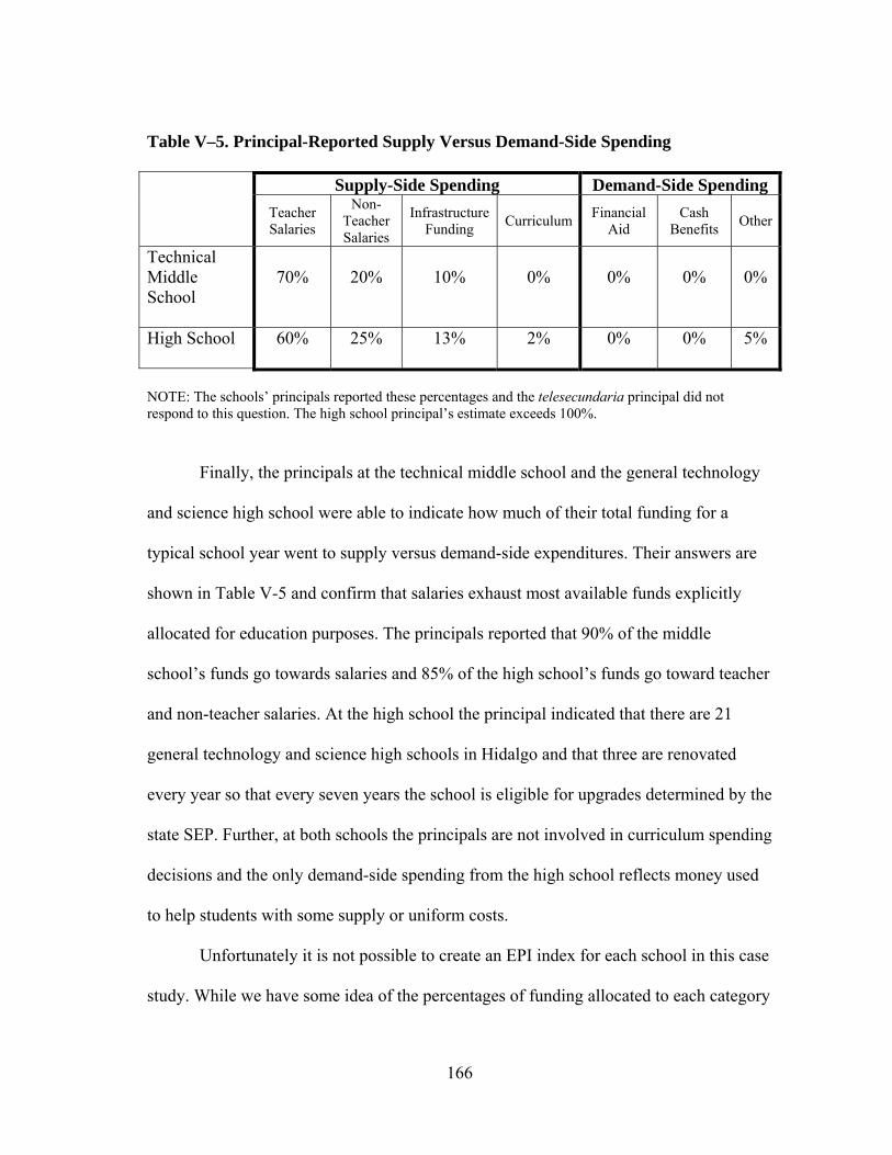
166

Table V–5. Principal-Reported Supply Versus Demand-Side Spending

Supply-Side Spending Demand-Side Spending

Teacher Salaries

Non-Teacher Salaries

Infrastructure Funding

CurriculumFinancial

Aid Cash

Benefits Other

Technical Middle School

70% 20% 10% 0% 0% 0% 0%

High School

60% 25% 13% 2% 0% 0% 5%

NOTE: The schools’ principals reported these percentages and the telesecundaria principal did not respond to this question. The high school principal’s estimate exceeds 100%.

Finally, the principals at the technical middle school and the general technology

and science high school were able to indicate how much of their total funding for a

typical school year went to supply versus demand-side expenditures. Their answers are

shown in Table V-5 and confirm that salaries exhaust most available funds explicitly

allocated for education purposes. The principals reported that 90% of the middle

school’s funds go towards salaries and 85% of the high school’s funds go toward teacher

and non-teacher salaries. At the high school the principal indicated that there are 21

general technology and science high schools in Hidalgo and that three are renovated

every year so that every seven years the school is eligible for upgrades determined by the

state SEP. Further, at both schools the principals are not involved in curriculum spending

decisions and the only demand-side spending from the high school reflects money used

to help students with some supply or uniform costs.

Unfortunately it is not possible to create an EPI index for each school in this case

study. While we have some idea of the percentages of funding allocated to each category

167

of supply-side spending, it is not known how much money is actually being spent. On

the demand side of the EPI equation, the number of students receiving benefits is known

but other benefits going to their families are unknown thus the needed data are

unavailable. What we do know, however, is that some students are receiving a particular

cash benefit that is means-tested and that this could be contributing to their social and

subsequently human capital development in addition to the resources available at their

school.

Section 5.6. Student Attitudes Towards Their Schools and Career Plans

To determine what students thought about the usefulness of their school, they

were asked seven questions. Four questions (question 5a through 5d) asked them if they

totally agreed, agreed, disagreed, or totally disagreed with the following four statements:

1) School has done little to prepare me for adult life when I leave school

2) School has been a waste of time

3) School has helped give me confidence to make decisions

4) School has taught me things which could be useful in a job

On average, students responded that school has taught them skills they would use

in a job and that they gained confidence from their experience; only 3% felt that school

was a waste of time or that it did not help them gain the skills they needed for a career.

While the majority saw school as an advantage, as many as 30% of students felt school

168

did not prepare them for adult life and some 10% felt that school did not help them gain

the confidence they needed to make good decisions.

Question 6 is an open-ended question and asks students to consider what specific

skills or knowledge they had gained in school that could be useful in a job and the

overwhelming majority of students felt that having an area of study, gaining a vocational

skill, was the biggest advantage for coming to school. Second was general knowledge or

subjects outside of their area of study, and third was learning self-confidence and being

respectful or getting along with others. The fourth most popular response was that they

learned a lot about technology and computers. Learning English was not important to

most students but it was mentioned enough to be in the top five. Some specific skills that

were noteworthy responses include time management, animal care, cooking, and

landscape drawing.

Questions 10 and 11 asked students to consider what they liked most and least

about their educational experience at school. Every student mentioned that they liked

learning something new or socializing with their friends. Playing soccer was also

mentioned frequently. The least liked aspects of school were studying math and getting

too much homework. A close third were complaints about teachers. Either teachers were

not showing up at all, they had meetings during class time, or they had a negative

attitude towards the students. One respondent wrote that, “Sometimes not everyone

complies with the rules of the school – neither the students nor the teachers.” Mean or

bullying students, uniforms, even nail inspections made the list of the least liked aspects

of the schools. Throughout the comments the issue of respect repeatedly surfaced. There

169

is a general attitude among students that learning to respect elders, others, and ones self

is an integral part of what one learns in school, and this was much lauded by students at

all three schools.

To evaluate students’ expectations of their academic and professional future,

survey respondents were asked about their plans in two ways. Question 7 asked students

to consider what they planned to do after they graduated in terms of more schooling or

professionally, and question 12 asked them to consider what they wanted to be when

they grew up. These two questions allowed for responses to be validated and gave space

for respondents to consider their answers more fully. Of the high school students who

responded to the survey 77% articulated a career choice and they overwhelmingly were

interested in the jobs they were currently preparing for (nursing, auto mechanics, or

computer networking) even if they indicated that they wanted to continue their

education. Approximately 30% wanted to pursue higher education to work in more

selective jobs that required more advanced university degrees (e.g., medical doctors or

lawyers).

Middle school students had a much harder time describing their future plans

beyond high school. From the technical and telesecundaria middle schools, of those

students that responded to questions 7 and 12 with a particular career in mind, the

majority sought highly selective jobs that require high-level degrees.

To compare students’ job aspirations against peers as well as their parents, all

jobs mentioned by survey respondents have been organized into 5 categorizes. The

lowest category is a “1” and includes jobs that do not require any literacy or education,

170

namely domestic and field labor work. Category “2” includes vendors, building

assistants and farmers – jobs that require a low level of math and Spanish literacy. Those

jobs in category “3” include jobs that require technical know-how and a fair amount of

literacy (e.g., mechanics, plumbers, and carpenters). Category “4” is for jobs that require

further schooling or certification such as police officers, teachers, nurses, or accountants.

Lastly, category “5” is for those professions that require extensive schooling and

cognitive skill: professors, lawyers, engineers, doctors, and architects. Appendix 5F

summarizes each category and lists the professions that were explicitly mentioned by

survey respondents.

The challenge of establishing an occupational hierarchy is multifaceted. The

approach taken for this chapter is based on education and cognitive requirements for the

jobs under consideration. Past literature has used composite socioeconomic indexes

based on “three measures of occupational standing: educational level, wage rate, and

prestige” (Hauser and Warren 1997, 225). In the Hauser and Warren (1997) analysis

cited above, the authors make the case that a job’s required educational level is more

important to determine a job’s occupational standing than the prestige and wage factors

– both of which can be highly variable over time and location. In addition to education

level requirements, however, the categories in this chapter also consider the necessary

aptitudes and skills a job demands. To discuss the details of a job’s skill requirements,

researchers used to look to the now defunct Dictionary of Occupational Titles or DOT

(Hartog 2000). This dictionary listed job requirements based on interviews with human

resource personnel as well as people who held the job under review. The DOT has been

171

replaced by O*NET – an online database maintained by the U.S. Department of Labor –

and provides occupation details such as skill and experience requirements, and the types

of tasks workers have to perform on the job. Given that this analysis is geared towards

careers in rural Mexico, however, this guide was not particularly useful for occupational

categorization.

In 2008 the International Labor Office (ILO) of the United Nations asked experts

on labor statistics to update the International Standard Classification of Occupations

(ISCO). While this classification is extensive it does not reflect a job hierarchy based on

skill or salary, nor does it offer occupational information such as job requirements. The

ISCO does, though, provide a useful outline for job categories. The occupational

categories used in this chapter are based on the ISCO and considers the current jobs held

by the parents of students who participated in the survey as well as students’ career

aspirations. Given the current employment opportunities in Calnali, Hidalgo, as well as

the educational offerings available to its population, the ordered occupational categories

created for this chapter captures the regional character and indicates, as the numbers on

the scale increase, upward mobility for workers.

The argument in this dissertation is that the demand-side spending that helps

students get to a school is critical for enabling students who would otherwise drop out,

but this type of spending is beyond the purview of individual schools. The only way to

assess demand-side spending impacts on building social and human capital at the

individual level, therefore, is to evaluate students who do benefit from the policies and to

see how they compare to their classmates who do not receive the benefit.

172

Section 5.7. Survey Data Analysis

Hypothesis 5.1 claims that middle school student who benefit from

Oportunidades are at least as likely as their peers who do not benefit from

Oporutnidades to go on to high school. At the telesecundaria in Papatlatla, 80% of

students receive Oportunidades and of those who do not receive the benefit (7 of the 37

students), more of them do not want to go on to high school (question 7 of the student

survey). A cross-tabulation (see Table V-6), shows that there is a significant correlation

(P= .004) between the telesecundaria students who receive Oportunidades and those

who plan to go on to high school.

For this population, a group more disadvantaged than the technical middle school

students, hypothesis 5.1 holds and the students who benefit from Oportunidades are

more likely than their peers who do not benefit from Oportunidades to go on to high

school. At the technical middle school in Calnali, however, 89% of students plan to go

on to high school and this does not have a significant correlation with whether or not the

students receive Oportunidades benefits. As more middle school students in a population

decide to pursue a high school diploma, the effect of Oportunidades may be less about

influencing such decisions as it is about helping students to have the same options as

their wealthier peers.

173

Table V–6. Telesecundaria and Technical Middle School Students and Their Plans for High School

Telesecundaria students* Technical middle school students** Does not

receive Oportunidades

Receives Oportunidades

Total

Percent Receiving

Oportunidades

Does not receive

Oportunidades

Receives Oportunidades

Total

Percent Receiving

OportunidadesNo

high school plans

4 3 7 43% 2 5 7 71%

High School plans

3 27 30 90% 25 30 55 55%

Total 7 30 37 81% 27 35 62 56% NOTE: All Telesecundaria students responded to this question whereas one technical middle school student did not. *Pearson X2 = 8.22, P= .004 ** Pearson X2 = .72, P= .40

174

At the high school level, 78% of all student respondents indicated that they

wanted to pursue more schooling. The correlation between whether or not a student

received Oportunidades and his or her desire for more education was barely significant

(P=.10) but it does indicate that students who are able to stay in school thanks to

Oportunidades are as likely as their peers to want to pursue higher education. Table V-7

shows this tabulated correlation.

Table V–7. Surveyed High School Students and Their Plans for Higher Education

Does not receive Oportunidades

Receive Oportunidades

Total Percent Receiving

OportunidadesNo plans for higher level

degree/university

5 24 29 83%

Plans to go on to higher level

degree/university University

34 69 103 67%

Total 39 93 132 70% NOTE: All high school students responded to this question. Pearson X2 = 2.70, P= .10

Hypothesis 5.2: Female middle school students who benefit from Oportunidades are at least as likely as their male counterparts to go on to high school Looking at just the students who receive Oportunidades at all of the schools

surveyed, 58% of the telesecundaria beneficiaries are girls, 67% are girls at the technical

middle school, and at the high school, 59% of beneficiaries are girls. In the

175

telesecundaria all of the 20 girls in the graduating class (100% of the female students)

receive cash transfers. Overall, at the middle schools and the high school surveyed,

among Oportunidades beneficiaries there is no statistically significant relationship

between the sex of students and their desire to continue their education. This could mean

that there is a negligible gender gap for beneficiaries and that the opportunities for

education at the middle and high school levels in this region are equalizing. In other

words, female Oportunidades students may be just as likely as male Oportunidades

students to stay in (or leave) school. However, with such a small sample this would need

to be validated in future studies with larger populations.

At the high school level, however, there is a statistical difference between girls

who receive cash transfers and those who do not (See Table V-8). Of the graduating girls

in the high school, 70% receive Oportunidades benefits and there is a statistically

significant relationship (P=.04) between receiving cash benefits and their desire for more

education. One explanation for this is that at the high school the students who are

registered in nursing are all female, and nearly all want to become nurses or another type

of medical professional, and all of these occupations require more schooling.

176

Table V–8. Is There a Difference Between Graduating Female High School

Students Who Get Cash Transfers and Those That Do Not?

Graduating Female students

who do not receive Oportunidades

Graduating Female students

who receive Oportunidades

Total

No plans for higher level

degree/university 1 13 14

Plans to go on to higher level

degree/university University

17 32 49

Total 18 45 63 *Pearson X2 = 4.05, P = .04

Looking more broadly at the middle school population, without considering

which students are receiving demand-side policy benefits, there is a significant

relationship between the sex of the student and whether or not they plan to go on to high

school. The results of the analysis are shown in Table V-9 for both middle schools

(telesecundaria, P=.02; the technical middle school, P=.08). What appears to be driving

the relationship is that there are more boys deciding to go to work instead of pursuing

high school.

177

Table V–9. Middle School Gender Differences in High School Aspirations

Telesecundaria Technical Middle School Females Males Females Males

No plans for High School

1 6 1 6

Plans for High School

19 11 26 27

20 17 27 33

Pearson X2 = 5.50 P= .02

Pearson X2 = 3.02 P= .08

Hypothesis 5.3: Middle school students who benefit from Oportunidades are at least as likely as their peers who do not benefit from Oportunidades to want to attain a higher level of education than their parents

Most students in school in rural Mexico exceed their parents’ level of education

if they go to high school and usually they match their parents’ education by completing

middle school. (As mentioned earlier, the average level of education in this region is

sixth grade). Of the students surveyed, no students at the telesecundaria reported having

a mother with an education level above middle school. The education level of mothers is

of particular importance since it often serves as an indicator for students’ academic

advantages that stem from the home learning environment a mother can provide.

Research has shown that there is usually a strong positive correlation between “mothers’

educational attainment and children’s test scores, academic outcomes, and cognitive

development” (Magnuson 2007, 1497). Table V-10 shows the telesecundaria students’

expectations and their parents’ education level regardless of their receipt of

Oportunidades.

178

Table V–10. Influences of Parents’ Education Level on all Telesecundaria

Students’ Academic Expectations (Regardless of Whether or Not They Receive

Oportunidades)

Mother’s Education Level* Total

No

School Elementary

School Middle School

High School

College/University

No high school plans

4 2 1 0 0 7

High School plans

12 14 4 0 0 30

Total 16 16 5 0 0 37 Father’s Education Level** Total

No

School Elementary


High School

College/University


5 0 2 0 0 7

High School plans

10 13 4 1 1 29

Total 15 13 6 1 1 36 NOTE: One student did not respond to the father’s education level question (37 telesecundaria students participated). * Pearson X2 = .82, P= .66 ** Pearson X2 = 6.2, P= .18

Since fathers are less reliably a part of the home life, their influence beyond

fiscal contribution is not usually discussed in the literature. For the telesecundaria

sample, 94% of the fathers have no more than a middle school education – one father

had completed high school and one other father had completed some sort of college

degree. Regardless of whether or not the student at the telesecundaria benefitted from

179

Oportunidades, the lack of variation in parents’ education level yielded no results for

this population. Essentially none of the parents are educated and so a student’s plans to

further his or her education is coming from other influences. It could be that students

realize that education matters for economic gain and perhaps the cash benefit of

Oportunidades is incentivizing them to continue their education. Based on some of the

responses to the open-ended questions on the surveys, there is a general appreciation for

education and the gains it can bring.

Seventy-five percent of the students in the technical middle school who

responded to the survey have parents who did not go on to high school and some 40%

have parents who did not go beyond elementary school. More mothers of students in the

middle school did go on to high school and college than fathers, but there is no

relationship between mothers’ education level and students’ desire for more school.

However, for this population there is a slightly significant (P=.09) relationship between

the fathers’ education level and students’ planning to get more education. This may

indicate that, in this region at least, fathers are having an influence on their children (See

Table V-11 for the detailed analysis). There are two students who, even though their

fathers pursued an education beyond high school, decided to stop their education after

middle school. In these cases they may not see the advantage of more schooling since

their fathers were not able to capitalize on their investment in education. Since most

mothers did not go beyond high school and most students want to pursue higher

education, there is not enough variation to determine if there is a relationship between

mothers’ education levels and students’ education plans.

180

Table V–11. Influence of Parents’ Education Level on all Technical Middle School

Students’ Academic Expectations (Regardless of Whether or Not They Receive

Oportunidades)


No

School Elementary


High School

College/ University


2 1 1 1 2 7

High School plans

7 15 20 7 5 54


No

School Elementary


High School

College/ University


2 2 0 0 3 7

High School plans

8 13 20 5 6 52

Total 10 15 20 5 9 59

NOTE: Not all students responded to these questions (63 technical middle school students participated). * Pearson X2 = 4.00, P= .35 ** Pearson X2 = 8.00, P= .09

Looking at just the Oportunidades beneficiaries in the technical middle school,

however, there is a significant relationship between both mother and fathers’ education

attainment and students’ expectations to go on to high school (See Table V-12). The

pattern is stronger for mothers’ education attainment as theory would suggest, and this

implies that among the poorest students in these rural communities, a push for more

education for girls especially has the potential to positively impact future generations.

This does not mean that fathers do not model for their sons the importance of education.

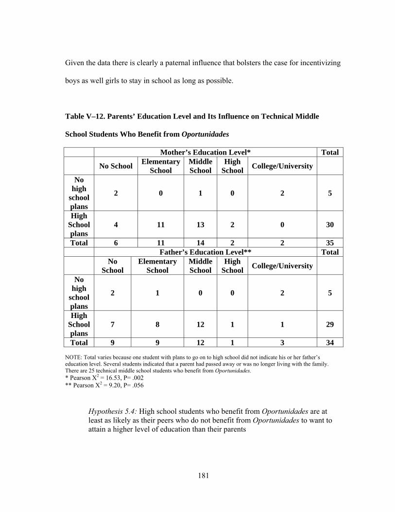
181

Given the data there is clearly a paternal influence that bolsters the case for incentivizing

boys as well girls to stay in school as long as possible.

Table V–12. Parents’ Education Level and Its Influence on Technical Middle

School Students Who Benefit from Oportunidades


No School Elementary


High School

College/University

No high

school plans

2 0 1 0 2 5

High School plans

4 11 13 2 0 30


No

School Elementary


High School

College/University

No high

school plans

2 1 0 0 2 5

High School plans

7 8 12 1 1 29

Total 9 9 12 1 3 34 NOTE: Total varies because one student with plans to go on to high school did not indicate his or her father’s education level. Several students indicated that a parent had passed away or was no longer living with the family. There are 25 technical middle school students who benefit from Oportunidades. * Pearson X2 = 16.53, P= .002 ** Pearson X2 = 9.20, P= .056

Hypothesis 5.4: High school students who benefit from Oportunidades are at least as likely as their peers who do not benefit from Oportunidades to want to attain a higher level of education than their parents

182

Of the high school student respondents, 91% of their mothers and 86% of their

fathers went only as far as middle school. Another 5% of mothers and 8% of fathers

completed high school and more fathers than mothers completed college or a post-high

school degree. As for their own expectations, 88% of the high school student

respondents indicated that they plan to go on to some institution of higher learning. By

making it to the third year of high school, the students overwhelmingly exceeded their

parents’ academic achievements and appear to be aiming much higher academically.

Nearly all respondents, regardless of whether they receive Oportunidades, indicated that

they saw education as key for a prosperous future.

Hypothesis 5.5: Male high school students who benefit from Oportunidades will be at least as likely as their peers who do not benefit from Oportunidades to seek nonagricultural jobs

The size of the surveyed population that is male, in high school, and indicated a

career is small (N=35), yet revealing. Only one student planned to pursue a level-1

occupation (those jobs that are agricultural in nature). Level-2 jobs could be agricultural

in nature as well (a rancher or farmer), but not one student indicated plans to pursue a

level-2 occupation. The overwhelming majority of students, 86%, indicated that they

wanted level-3 or level-4 jobs showing that in fact, all students, regardless of whether or

not they benefit from Oportunidades, are seeking higher paying, more prestigious jobs

that require more education.

183

Hypothesis 5.6: Students who go to technical middle schools are more likely to plan to go on to high school than students who go to telesecundaria middle schools

Of the students in the technical middle school who responded to the survey and

answered the questions about their educational plans (N=62), 89% planned to go on to

high school. All telesecundaria students (N=37) answered the survey questions and 81%

plan to continue on to high school. There is no statistical difference between the two

groups. What the surveys did reveal is that the students in Calnali’s technical middle

school mostly planned to pursue high school at the CECyTEH while those in Papatlatla

planned to go the COBAEH, a lower quality high school. Isolating the career

expectations of the students at each middle school was also not statistically different;

most students want level-4 or level-5 jobs. Only a longitudinal study would allow us to

see if students actually do what they claim they are going to do and where their goals

take them.


Without the demand-side policy of Oportunidades, most of the students at the

rural schools surveyed for this chapter would not be able to afford investing in

education. Living in poverty and having parents who have not gone past a middle-school

education limits students in many ways. What the analysis presented here shows is that

the investment in the poorest families has been paying off so that these students’

academic and professional choices are beginning to mirror those students who have

more advantages.

184

First we saw that middle school students who benefit from Oportunidades in

Calnali, Hidalgo in Mexico are just as likely and in some cases more likely than non-

beneficiaries to pursue a high school degree. Second, females are becoming just as likely

as their male classmates to pursue high school and even more likely to pursue a higher

level degree. This is significant for the next generation of students who should benefit

from having more educated mothers. Previous studies have addressed how

Oportunidades has helped girls stay in middle school and this study extends that

discussion to how Oportunidades impacts girls’ plans once they are in high school. One

high school nursing student who responded to the survey wrote that she wants to “work

in a health center, [and] also to study to specialize in something so that when I form a

family they receive the best.”62 This particular student’s mother is a stay at home mom

and her father had been a day laborer but had recently passed away. Both of her parents

had only finished elementary school. Clearly she has embraced the importance of

continuing her education so that she can provide for her future children.

Since most parents in this region did not finish middle school, students who are

completing middle and high school are surpassing them and Oportunidades is helping to

make that possible – adding to Mexico’s overall level of human capital. The type of jobs

students plan to pursue also surpasses their parents’ careers in terms of educational

requirements, prestige, and salary. All students in this region, not just male high school

students, are less likely to pursue work in agriculture. While it is not possible to know

what happens to these students without a more complete longitudinal study, it will be

62 Translated from the Spanish.

185

worthwhile to follow what happens economically in the region over the next ten years to

see if these policies are having an impact in the aggregate.

In conclusion, so long as the demand-side policies continue to aid the poorest

families so that sending their children to school remains their best economic option,

Mexico can focus its monies on the serious supply-side issues it faces including the

quality of the schools and teachers. Based on the findings in Chapter IV, we can also

conclude that Mexico needs to localize decision making so that schools can more easily

negotiate with officials for the things they need to effectively teach students.

186

CHAPTER VI

CONCLUSION: INSIGHTS GAINED, SUGGESTIONS FOR FUTURE

RESEARCH




dissertation expands the definition of education spending so that in addition to

expenditures allocated to schools (supply-side expenditures), it includes benefits that

help families participate in the education system (demand-side expenditures). The

simultaneous funding of both schools and family benefits, I argue, contributes both

directly and indirectly to the development of a country’s level of human capital, or

students’ level of marketable skills and knowledge. This dissertation presents compelling

evidence that both types of expenditures do make a difference for students – especially

those coming from the most disadvantaged circumstances.

In the introduction to this dissertation, I presented Figure I-1 as a response to W.

Norton Grubb’s call for a new model of schooling (Grubb 2009). The model I developed

shows how education spending is interconnected with political institutions and with the

ideology of government leadership (Chapter III). The model also indicates that spending

policies can have an incentivizing influence on families to send their students to school

as well as on the students who go, and funding can also have an effect on the quality of

187

the schools themselves (Chapters IV and V). At the heart of the model is the Education

Policy Index (EPI; Chapter II) that captures both traditional school spending as well as

family benefits. The approach presented in this dissertation recognizes the necessity of

both school (supply-side) and family (demand-side) policies for helping students

develop their human capital, and the final measure for everyone is how well prepared

students are for what awaits them after graduation. My finding that both supply- and

demand-side expenditures matter for the development of student skills and knowledge is

important because gains in human capital should have positive impacts on individual

students’ earnings potential, as well as for their country’s level of economic growth

(Grosh, et al. 2008; Woessmann and Hanushek 2012).

In Chapter II, I introduced the EPI as a spending indicator designed to reveal the

balance of a country’s expenditures on families relative to schools and teachers;

demand-side spending helps students access schools whereas supply-side spending is

indicative of the average quality of the country’s school system. The balance of these

two types of expenditures can be a useful tool for policy-makers who need to get an idea

of where fiscal resources are going, and can be used by researchers to assess the impact

spending is having on student outcomes. Further, the EPI serves as an innovative

measure for comparing how countries fund education and human capital development

more broadly. The EPI is also a novel way to assess what political factors are associated

with differing levels of education spending.

Countries’ level of wealth, inequality, and poverty do not have an impact on the

balance of the EPI scores. Rather, as discussed in Chapter III, political factors such as

188

the country’s electoral system, leadership ideology, and labor union power have a strong

influence over how redistributive a country’s policies will be and thus how much

spending will be allocated to demand-side policies. When the electoral system is a

proportional representative (PR) system, labor unions are able to influence demand-side

spending positively. Moreover, PR systems tend to redistribute more then majoritarian or

mixed systems, and left-learning governments also favor more generous demand-side

expenditures. Spending on family benefits and students is considered more redistributive

than spending on schools where all students, regardless of their family background or

wealth, can go to learn. One advantage of the EPI in analytical models is that it can help

identify which students are, based on demand-side benefits, making gains through the

school system.

An analysis in Chapter II shows that the rate of student resilience, the percentage

of students from a country’s bottom quartile on the SES spectrum to score in the top

quartile on the 2009 Programme for International Assessment (PISA) exam, was

positively correlated with higher EPI scores, i.e. higher investments in supply-side items

like school infrastructure. This finding indicates that supply-side spending in the

aggregate can make a difference for less advantaged students.

This is confirmed in Chapter IV when I analyze the impact of the EPI-M on

PISA exam results. The EPI-M, the ratio of supply-side spending to means-tested

demand-side spending only (see Chapter II for details), was positively correlated with

reading, science, and math PISA scores. When the three components of supply-side

spending were unpacked, spending on teachers’ compensation and non-compensation

189

expenditures had a positive impact on reading and math scores, while capital

expenditures positively impacted student performance on each of the PISA exams.

School expenditures thus appear to help disadvantaged students develop their human

capital as measured by exam performance. However, the two middle-income countries in

the dataset with a high EPI, Mexico and Brazil, are not getting desirable results on the

PISA exams despite a strong investment in schools and teachers. The spending on

schools is evidently not producing results; one contributing factor may be corruption

with respect to expenditures on school infrastructures and teacher salaries.63 A more

detailed investigation of where the money actually goes in these countries would help to

reveal spending inefficiencies.

The findings in this dissertation support the argument that formal schooling can

help students across the SES spectrum gain useful skills and knowledge (Hedges, et al.

1994; Nye, et al. 2004). If schools are important, then it is key that students actually go

to school. In Chapter V, which provided case studies of three schools in a poor

municipality, Calnali, in rural Mexico, many students benefit from a federal means-

tested conditional cash transfer (CCT) program called Oportunidades that benefits about

a quarter of Mexico’s population. To receive benefits, families must meet a myriad of

requirements that include getting their students to school 85% of the time. Students

63 Several measures of corruption confirm that within the dataset used throughout the dissertation, Brazil and Mexico have the highest levels of corruption. The measures are Transparency International’s Corruption Perceptions Index and the Political Risk Services group’s International Country Risk Guide indicator of Quality of Government that combines corruption, law and order, and bureaucracy quality measures. In February 2013, Elba Esther Gordillo, the head of the Mexican teachers’ union, Sindicato Nacional de Trabajadores de la Educación, or SNTE, was arrested on embezzlement charges adding to concerns that the teachers union in particular is misusing funds.

190

receiving Oportunidades in Calnali overwhelmingly indicated that they would not be

able to attend middle or high school were it not for fiscal assistance. Indeed, across

countries, demand-side spending is positively correlated with enrollment rates (Chapter

IV).

Further, in the case studies presented in Chapter V, the student beneficiaries of

the means-tested cash benefits indicate on surveys that their academic and professional

goals are comparable to those of their more advantaged classmates; in some cases their

plans even exceed those of their classmates. Girls, even more than boys, are positively

impacted by such expenditures and have greater academic expectations. With the known

influence of mothers’ level of education on their children’s futures, this has the potential

to increase levels of human capital development in Mexico (Magnuson 2007).

Section 6.1. Suggestions for Future Research

This dissertation shows the utility of measuring education expenditures in a way

that includes both supply- and demand-side spending, which is a novel contribution to a

literature that has long measured education spending as only supply-side spending.

However, this project also leaves many questions unanswered and points to many

fruitful directions for further research.

If more nuanced spending measures were available at the national level so that

the supply-side and demand-side expenditures could be unpacked even further, we could

better understand how these spending initiatives matter. For example, gross teacher

compensation levels could reflect that either fewer teachers are paid more, or that there

191

are more teachers being paid less. These distinctions are not possible with the data used

throughout this dissertation. Further, due to the nature of the data available (i.e., the

countries that participate in the PISA exams and that make government expenditures

data available), I sampled only wealthy and high-middle income countries. Studying the

full spectrum of global economic development would allow greater exploration of how

both demand- and supply-side spending interact and impact student performance in cases

where a large percentage of students would not be likely to enroll in, or stay in school if

the government did not aggressively make policy to include them. In less developed

countries especially such policies are often influenced by investments from international

sources such as the World Bank or the International Monetary Fund.

Most of the countries in this dataset are wealthy and only four (Turkey, Mexico,

Chile, and Brazil) have major loans from the World Bank, other countries, or other

international monetary funding sources. These loans are important for funding the

means-tested demand-side programs, such as conditional cash transfers, that are part of

the EPI. Many other countries have adopted similar cash transfer programs that target

getting children to enroll in, and stay in school, so there are additional countries that

could be included in future analyses, though most of those countries are not participants

in the PISA testing program and data from these countries are not always available due

to a lack of fiscal transparency.

A longitudinal study that would follow students from middle through high

school, and on to either vocational school or university, and finally into the workplace,

would provide a great deal more insight into how much human capital is being

192

developed within these institutions. Vocational schools are especially germane to this

research topic given their intent to train students for specific careers. A possible model is

the National Child Development Study in Great Britain that follows a cohort of children

who were born in one week in 1958. By the age of 16, students from this cohort were

able to fairly accurately predict their first job after graduating from school (Brown, et al.

2011). Such a dataset in a country with available government expenditures data would

make it possible to assess the effectiveness of different spending categories on human

capital development.

In Chapter IV I extended the research on human capital development from strict

measures of spending to the level of government that actually makes education policy

decisions. Concentration of decision making at the national level clearly showed a

negative impact on PISA exam results, while decision-making at the local was the most

promising for student outcomes. It would be interesting to delve further into this finding

and to interview local-level decision makers in countries that are having the best success.

Finally, there are two things that were not incorporated into the EPI: taxation

policy and private expenditures on public institutions. The EPI did not, for example,

account for tax credits as part of a voucher system that helps fund families sending their

children to government-dependent private schools (as in Germany and Portugal). Future

constructions of the EPI should find ways to account for these variations between

countries since these differences may impact the balance of spending.

United Nations Secretary-General Ban Ki-Moon wrote “The power of education

to transform lives is universal. When you ask parents what they want for their children—

193

even in war zones and disaster areas—they seek the same thing first: education. Parents

want their children in school” (Ki-moon September 2012). To meet this demand,

governments can allocate funds to families in their society that most need support, and

simultaneously make sure that the schools students experience are worth the effort to get

there. Both investments are necessary for a thriving economy and a self-sustaining

population. This dissertation contributes to our understanding of how the “package” of

education spending, broadly defined, impacts students and by extension human capital

development.

194

REFERENCES

Adema, Willem. 2006. “Social Assistance Policy Development and the Provision of a Decent Level of Income in Selected OECD Countries.” In OECD Social Employment and Migration Working Papers No. 38. Paris: Organisation for Economic Cooperation and Development.

Altinok, Nadir. 2008. “An International Perspective on Trends in the Quality of

Learning Achievement (1965-2007).” Paper commissioned for the EFA Global Monitoring Report 2009, “Overcoming Inequality: Why Governance Matters.”

Alvarez, Jesus, Vicente Garcia Moreno, and Harry A. Patrinos. 2007. “Institutional

Effects as Determinants of Learning Outcomes: Exploring State Variations in Mexico.” World Bank Policy Research Working Paper No. 4286 World Bank, Washington, D.C. http://ssrn.com/abstract=1004200.

Ansell, Ben W. 2008. “Traders, Teachers, and Tyrants: Democracy, Globalization, and

Public Investment in Education.” International Organization 62: 289-322. ______. 2010. From the Ballot to the Blackboard: The Redistributive Political

Economy of Education. New York: Cambridge University Press. Arts, Wil, and John Gelissen. 2002. “Three Worlds of Welfare Capitalism or More? A

State-of-the-Art Report.” Journal of European Social Policy 12: 137-58. Attanasio, Orazio p., Costas Meghir, and Ana Santiago. 2011. “Education Choices in

Mexico: Using a Structural Model and a Randomized Experiment to Evaluate Progresa.” The Review of Economic Studies. http://restud.oxfordjournals.org/content/early/2011/08/02/restud.rdr015.abstract

Aud, S., W. Hussar, F. Johnson, G. Kena, E. Roth, E. Manning, X. Wang, and J. Zhang.

2012. “The Condition of Education 2012 (NCES 2012-045).” U.S. Department of Education, National Center for Education Statistics, Washington, D.C. http://nces.ed.gov/pubsearch.

Avelino, George, David S. Brown, and Wendy Hunter. 2005. “The Effects of Capital

Mobility, Trade Openness, and Democracy on Social Spending in Latin America, 1980-1999.” American Journal of Political Science 49: 625-41.

Bardhan, Pranab. 2002. “Decentralization of Governance and Development.” The

Journal of Economic Perspectives 16: 185-205. Barrera-Osorio, Felipe, Tazeen Fasih, Harry Anthony Patrinos, and Lucrecia Santibáñez.

2009. “Decentralized Decision-Making in Schools: The Theory and Evidence

195

on School-Based Management.” Washington, D.C.: The International Bank for Reconstruction and Development/The World Bank.

Becker, Gary S. 1962. “Investment in Human Capital: A Theoretical Analysis.” The

Journal of Political Economy 70: 9-49. ______. 1992. “Human Capital and the Economy.” Proceedings of the American

Philosophical Society 136: 85-92. Becker, Gary S, and Nigel Tomes. 1986. “Human Capital and the Rise and Fall of

Families.” Journal of Labor Economics 4: S1-S39. Behrman, J., Piyali Sengupta, and P. Todd. 2000. “Final Report: The Impact of

Progresa on Achievement Test Scores in the First Year.” International Food Policy Research Institute, Processed., Washington, D.C. http://evaluacion.oportunidades.gob.mx:8010/441c7c1a3d30adf64e0e724174a9d527/impacto/2000/ifpri_2000_bherman_archive.pdf.

Behrman, Jere R., Jorge Gallardo-García, Susan W. Parker, Petra E. Todd, and Viviana

Vélez-Grajales. 2012. “Are Conditional Cash Transfers Effective in Urban Areas? Evidence from Mexico.” Education Economics 20: 233-59.

Behrman, J.R., S.W. Parker, and P.E. Todd. 2005. “Long-Term Impacts of the

Oportunidades Conditional Cash Transfer Program on Rural Youth in Mexico.” Germany: Discussion paper Nr122 for the Ibero-America Institute for Economic Research.

Behrman, Jere R., Susan W. Parker, and Petra E. Todd. 2009. “Medium-Term Impacts

of the Oportunidades Conditional Cash-Transfer Program on Rural Youth in Mexico.” In Poverty, Inequality, and Policy in Latin America, eds. Stephan Klasen and Felicitas Nowak-Lehmann. Cambridge, MA: The MIT Press. 219-70.

______. 2011. “Do Conditional Cash Transfers for Schooling Generate Lasting

Benefits? A Five-Year Followup of Progresa/Oportunidades.” The Journal of Human Resources 46: 93-122.

Behrman, Jere R., and Emmanuel Skoufias. 2006. “Mitigating Myths About Policy

Effectiveness: Evaluation of Mexico’s Antipoverty and Human Resource Investment Program.” The ANNALS of the American Academy of Political and Social Science 606: 244-75.

196

Bloom, Erik, Gladys López-Acevedo, Andreas Blom, Andrew Mason, and Alexis Roach. 2007. “Chapter 7: Human Capital and Skills for a Competitive Labor Market.” In Mexico 2006-2012: Creating the Foundations for Equitable Growth, ed. David Rosenblatt. Vol. Report No. 39993-MX. Mexico: The World Bank. 213 - 46.

Boix, Carles. 1997. “Political Parties and the Supply Side of the Economy: The

Provision of Physical and Human Capital in Advanced Economies, 1960-90.” American Journal of Political Science 41: 814-45.

Brady, Henry E., Sidney Verba, and Kay Lehman Schlozman. 1995. “Beyond SES: A

Resource Model of Political Participation.” The American Political Science Review 89: 271-94.

Braine, Theresa. 2006. “Reaching Mexico's Poorest.” Bulletin of the World Health

Organization. http://www.scielosp.org/scielo.php?script=sci_arttext&pid=S0042-96862006000800004&nrm=iso. (November 7, 2012).

Breen, Richard. 1997. “Inequality, Economic Growth and Social Mobility.” The

British Journal of Sociology 48: 429-49. Brown, David S., and Wendy Hunter. 2004. “Democracy and Human Capital

Formation: Education Spending in Latin America, 1980 to 1997.” Comparative Political Studies 37: 842-64.

Bruhn, Kathleen. 1996. “Social Spending and Political Support: The ‘Lessons’ of the

National Solidarity Program in Mexico.” Comparative Politics 28: 151-77. Bryson, Lois, Michael Bittman, and Sue Donath. 1994. “Men's Welfare State, Women's

Welfare State: Tendencies to Convergence in Practice and Theory?” In Gendering Welfare States, ed. D. Sainsbury. London: Sage. 118-31.

Busemeyer, Marius R. 2007. “Determinants of Public Education Spending in 21 OECD

Democracies, 1980-2001.” Journal of European Public Policy 14: 582-610. ______. 2008. “Social Democrats and the New Partisan Politics of Public Investment in

Education.” Journal of European Public Policy 16: 107-26. ______. 2009. “Social Democrats and the New Partisan Politics of Public Investment in

Education.” Journal of European Public Policy 16: 107-26. Castelló-Climent, Amparo. 2008. “On the Distribution of Education and Democracy.”

Journal of Development Economics 87: 179-90.

197

Castles, Francis G. 2009. “What Welfare States Do: A Disaggregated Expenditure

Approach.” Journal of Social Policy 38: 45--62. Cecchini, Simone, and Aldo Madariaga. 2011. “Conditional Cash Transfer

Programmes: The Recent Experience in Latin America and the Caribbean.” Santiago, Chile: United Nations.

Chubb, John E., and Terry M. Moe. 1988. “Politics, Markets, and the Organization of

Schools.” The American Political Science Review 82: 1066-87. ______. 1990. Politics, Markets, and America's Schools. Washington, D.C.: The

Brookings Institution. Coady, David P., and Susan W. Parker. 2004. “Cost-Effectiveness Analysis of

Demand- and Supply-Side Education Interventions: The Case of PROGRESA in Mexico.” Review of Development Economics 8: 440-51.

Coleman, James S. 1988. “Social Capital in the Creation of Human Capital.” The

American Journal of Sociology 94, Supplement: Organizations and Institutions: Sociological and Economic Approaches to the Analysis of Social Structure: S95-S120.

Coleman, James S., Ernest Q. Campbell, Carol J. Hobson, James McPartland, Alexander

M. Mood, Frederic D. Weinfeld, and Robert L. York. 1966. “Equality of Educational Opportunity.” Washington, D.C.: Government Printing Office.

Condron, Dennis J. 2011. “Egalitarianism and Educational Excellence: Compatible

Goals for Affluent Societies?” Educational Researcher 40: 47-55. Cusack, Thomas R. 1997. “Partisan Politics and Public Finance: Changes in Public

Spending in the Industrialized Democracies, 1955-1989.” Public Choice 91: 375-95.

de Janvry, Alain, Frederico Finan, Elisabeth Sadoulet, and Renos Vakis. 2006. “Can

Conditional Cash Transfer Programs Serve as Safety Nets in Keeping Children at School and from Working When Exposed to Shocks?” Journal of Development Economics 79: 349-73.

Diaz-Cayeros, Alberto, Federico Estévez, and Beatriz Magaloni. 2012. “Strategies of

Vote Buying: Democracy, Clientelism and Poverty Relief in Mexico.” http://www.stanford.edu/~magaloni/dox/2012strategiesvotebuying.pdf. Accessed November 12, 2012.

198

Dohn, Nina Bonderup. 2007. “Knowledge and Skills for PISA—Assessing the

Assessment.” Journal of Philosophy of Education 41: 1-16. Dolton, Peter, and Oscar D. Marcenaro-Gutierrez. 2011. “If You Pay Peanuts Do You

Get Monkeys? A Cross-Country Analysis of Teacher Pay and Pupil Performance.” Economic Policy 26: 5-55.

Downey, Douglas B., T. von Hippel Paul, and Beckett A. Broh. 2004. “Are Schools the

Great Equalizer? Cognitive Inequality During the Summer Months and the School Year.” American Sociological Review 69: 613-35.

ECLAC. 2011. “Non-Contributive Social Program Database in Latin America and the

Caribbean.” Social Development Division of the Economic Commission for Latin America and the Caribbean (ECLAC). http://dds.cepal.org/bdptc/programa/?id=22. (Accessed November 6, 2012).

Elizondo Mayer-Serra, C. 2009. “Perverse Equilibria: Unsuitable but Durable

Institutions.” In No Growth without Equity? Inequality, Interests and Competition in Mexico, eds. S. Levy and M. Walton: The World Bank and Palgrave Macmillan.

Esping-Andersen, Gøsta. 1990. The Three Worlds of Welfare Capitalism. Princeton:

Princeton University Press. EUROSTAT. 2008. “Esspros Manual, the European System of Integrated Social

Protection Systems (Esspros).” http://ec.europa.eu/eurostat/ramon/statmanuals/files/KS-RA-07-027-EN.pdf.

Fernald, Lia C.H., Paul J. Gertler, and Lynnette M. Neufeld. 2008. “Role of Cash in

Conditional Cash Transfer Programmes for Child Health, Growth, and Development: An Analysis of Mexico’s Oportunidades.” Lancelot 371: 828-37.

Fierro, C.E., G. Tapia García, and F. Rojo Pons. 2009. “Descentralización Educativa en

México: Un Recuento Analítico.” Paper prepared for the OECD in the context of the project “Implementación de Políticas Educativas”.

Fiszbein, Ariel, and Norbert Schady. 2009. Conditional Cash Transfers: Reducing

Present and Future Poverty. Washington, D.C.: The World Bank. Förster, M., and G. Verbist. 2012. “Money or Kindergarten? Distributive Effects of

Cash Versus Inkind Family Transfers for Young Children.” Vol. 135, OECD Social, Employment and Migration Working Papers: OECD Publishing.

199

Fuchs, Thomas, and Ludger Woessmann. 2007. “What Accounts for International

Differences in Student Performance? A Re-Examination Using PISA Data.” Empirical Economics 32: 433-64.

García, Adán Moisés, Yuriko Teresa Benítez Ríos, Edna Huerta Velásquez, Norma

Isabel Medina Mayagoitia, and Guadalupe Ruiz Cuéllar. 2007. “Infraestructura Escolar en las Primarias y Secundarias de México.” Instituto National para la Evaluación de la Educación (INEE). http://www.inee.edu.mx/sitioinee10/Publicaciones/InformesdeResultados/Condicionesdelaoferta/P1D231IEPRISECUMEX.pdf

Gertler, Paul J., Sebastian W. Martinez, and Marta Rubio-Codina. 2012. “Investing

Cash Transfers to Raise Long-Term Living Standards.” American Economic Journal: Applied Economics 4: 164-92.

Goldstein, Harvey. 2004. “International Comparisons of Student Attainment: Some

Issues Arising from the Pisa Study.” Assessment in Education: Principles, Policy & Practice 11: 319-30.

Gómez Hermosillo, R. 2011. “La Efectividad de las Redes de Protección Social: El Rol

de los Sistemas Integrados de Información Social en México.” Notas técnicas, No. 195 (IDB-TN-195). Washington, D.C.: Inter-American Development Bank (IDB).

Grindle, Merilee S. 2004. Despite the Odds: The Contentious Politics of Education

Reform. Princeton: Princeton University Press. Grubb, W. Norton. 2009. The Money Myth: School Resources, Outcomes, and Equity.

New York: The Russell Sage Foundation. Guardia, F. Hoces de la, A. Hojman, and O. Larrañaga. 2011. “Evaluating the Chile

Solidario Program: Results Using the Chile Solidario Panel and the Administrative Databases (Evaluando El Programa Chile Solidario: Resultados Usando El Panel Chile Solidario Y Datos Administrativos).” Estudios de Economía 38: 129-68.

Hanushek, Eric A. 1989. “The Impact of Differential Expenditures on School

Performance.” Educational Researcher 18: 45-62. ______. 1997. “Assessing the Effects of School Resources on Student Performance: An

Update.” Educational Evaluation and Policy Analysis 19: 141-64.

200

Hanushek, Eric A., and Ludger Woessmann. 2011. “How Much Do Educational Outcomes Matter in Oecd Countries?” Economic Policy 26: 427-91.

Harris, Alma, and Stewart Ranson. 2005. “The Contradictions of Education Policy:

Disadvantage and Achievement.” British Educational Research Journal 31: 571-87.

Hartog, Joop. 2000. “Over-Education and Earnings: Where Are We, Where Should We

Go?” Economics of Education Review 19: 131-47. Hartog, J. 2000. “The Overeducated Worker? The Economics of Skill Utilization.” In

Economics of Education Review, eds. Lex Borghans and Andries de Grip. Cheltenham, UK: Edward Elgar.

Hartog, Joop, and Wim Vijverberg. 2007. “Schools, Skills and Risk.” Economics of

Education Review 26: 758-70. Hauser, Robert M., and John Robert Warren. 1997. “Socioeconomic Indexes for

Occupations: A Review, Update, and Critique.” Sociological Methodology 27: 177-298.

Henisz, W. J. 2000. “The Institutional Environment for Economic Growth.”

Economics and Politics 12: 1-31. Henisz, Witold J. 2002. “The Institutional Environment for Infrastructure Investment.”

Industrial and Corporate Change 11: 355-89. Hibbs, A. 1992. “Partisan Theory after Fifteen Years.” European Journal of Political

Economy 8: 361-73. Hicks, Alexander, and Duane H. Swank. 1984. “Governmental Redistribution in Rich

Capitalist Democracies.” Policy Studies Journal 13: 265- 86. Holmlund, Helena, Sandra McNally, and Martina Viarengo. 2010. “Does Money

Matter for Schools?” Economics of Education Review 29: 1154-64. Hopkins, David, Elpida Ahtaridou, Peter Matthews, and Charles Posner. 2007. “An

Analysis of the Mexican School System in Light of PISA 2006.” London: OECD Directorate for Education.

Imbeau, Louis M., Francois Petry, and Moktar Lamari. 2001. “Left-Right Party

Ideology and Government Policies: A Meta-Analysis.” European Journal of Political Research 40: 1-29.

201

INEGI. 2010. “Censo De Población Y Vivienda 2010.” Instituto Nacional de Estadística y Geografía (INEGI).

Iversen, Torben, and David Soskice. 2006. “Electoral Institutions and the Politics of

Coalitions: Why Some Democracies Redistribute More Than Others.” American Political Science Review 100: 165-81.

______. 2009. “Distribution and Redistribution: The Shadow of the Nineteenth

Century.” World Politics 61: 438-86. Iversen, Torben, and John D. Stephens. 2008. “Partisan Politics, the Welfare State, and

Three Worlds of Human Capital Formation.” Comparative Political Studies 41: 600-73.

Jafarey, Saqib, and Sajal Lahiri. 2005. “Food for Education Versus School Quality: A

Comparison of Policy Options to Reduce Child Labour.” The Canadian Journal of Economics / Revue canadienne d'Economique 38: 394-419.

Jara, Felipe Hevia de la. 2008. “Between Individual and Collective Action: Citizen

Participation and Public Oversight in Mexico’s Oportunidades Programme.” Institute of Development Studies Bulletin 38.

Jencks, Christopher, Smith Marshall, Henry Acland, Mary Jo Bane, David Cohen,

Herbert Gintis, Barbara Heyns, and Stephanie Michelson. 1972. Inequality: A Reassessment of the Effect of Family and Schooling in America. New York: Basic Books.

Jensen, Carsten. 2011. “Capitalist Systems, Deindustrialization, and the Politics of

Public Education.” Comparative Political Studies 44: 412-35. Kan, Man Yee, and Jonathan Gershuny. 2006. “Human Capital and Social Position in

Britain: Creating a Measure of Wage-Earning Potential from Bhps [British Household Panel Survey] Data.” ISER Working Paper 2006-03. Colchester: University of Essex.

Kaufman, Robert R., and Alex Segura-Ubiergo. 2001. “Globalization, Domestic

Politics, and Social Spending in Latin America: A Time-Series Cross-Section Analysis, 1973-97.” World Politics 53: 553-87.

Keefer, Philip. 2010. “DPI 2010 - Database of Political Institutions: Changes and

Variable Definitions.” ed. Development Research Group. The World Bank.

202

Kolarič, Zinka, Anja Kopač Mrak, and Tatjana Rakar. 2011. "Welfare States in Transition: The Development of the Welfare System in Slovenia." In Welfare States in Transition: 20 Years after the Yugoslav Welfare Model, eds. Marija Stambolieva and Stefan Dehnert. Sofia, Bulgaria: Friedrich Ebert Foundation. 288-309.

Korpi, Walter. 2006. “Power Resources and Employer-Centered Approaches in

Explanations of Welfare States and Varieties of Capitalism: Protagonists, Consenters, and Antagonists.” World Politics 58: 167-206.

Lake, David A., and Matthew A. Baum. 2001. “The Invisible Hand of Democracy:

Political Control and the Provision of Public Services.” Comparative Political Studies 34: 587 - 621.

Lee, Jong-Wha, and Robert J. Barro. 2001. “Schooling Quality in a Cross-Section of

Countries.” Economica 68: 465-88. Levy, Santiago. 2006. “Progress against Poverty: Sustaining Mexico’s Progresa-

Oportunidades Program.” Washington, D.C.: Brookings Institute Press. Lindert, Kathy, Anja Linder, Jason Hobbs, and Bénédicte de la Brière. 2007. “The Nuts

and Bolts of Brazil’s Bolsa Família Program: Implementing Conditional Cash Transfers in a Decentralized Context.” Social Protection Discussion Paper No. 0709. The World Bank. http://siteresources.worldbank.org/SOCIALPROTECTION/Resources/SP-Discussion-papers/Safety-Nets-DP/0709.pdf.

Lindstrom, Lauren, Bonnie Doren, Jennifer Metheny, P. A. M. Johnson, and Claire

Zane. 2007. “Transition to Employment: Role of the Family in Career Development.” Exceptional Children 73: 348-66.

Lopez-Acevedo, Gladys. 2003. “A Reassessment of Technical Education in Mexico.”

Journal of Career and Technical Education 19: Electronic Journal. Magnuson, Katherine. 2007. “Maternal Education and Children's Academic

Achievement During Middle Childhood.” Developmental Psychology 43: 1497-512.

McBee, Robin Haskell. 2002. “When It Comes to Testing, Why Not Make

Lemonade?” Educational Forum 66: 238-46. Montt, Guillermo. 2012. “Does Money Buy Strong Performance in PISA?” PISA In

Focus. http://www.oecd.org/pisa/pisainfocus/. (March 5, 2012).

203

Muñoz-Izquierdo, C. 2007. “Educational Effects of the Compensatory Programs in Mexico.” In Universalization of Primary Education in the Historical Perspective, ed. Yonemura A. Japan: Institute of Developing Economies.

Murillo, Maria Victoria. 1999. “Recovering Political Dynamics: Teachers' Unions and

the Decentralization of Education in Argentina and Mexico.” Journal of Interamerican Studies and World Affairs 41: v-57.

N. Ozawa, Martha. 2004. “Social Welfare Spending on Family Benefits in the United

States and Sweden: A Comparative Study.” Family Relations 53: 301-09. Neyer, Gerda, and Gunnar Andersson. 2008. “Consequences of Family Policies on

Childbearing Behavior: Effects or Artifacts?” Population and Development Review 34: 699-724.

OECD. 2009a. “Education at a Glance.” Paris: OECD. ______. 2009b. “OECD Economic Surveys: Mexico 2009.” July 2009. Paris: OECD. ______. 2010a. “The High Cost of Low Educational Performance: The Long-Run

Economic Impact of Improving PISA Outcomes.” Paris: OECD. ______. 2010b. “PISA 2009 Results: Overcoming Social Background – Equity in

Learning Opportunities and Outcomes (Volume II).” Paris: OECD. ______. 2010c. “PISA: Programme for International Student Assessment.” OECD

Education Statistics (database). ______. 2010d. “OECD Factbook 2010: Economic, Environmental and Social

Statistics.” Paris: OECD. ______. 2010e. “PISA 2009 Results: What Makes a School Successful? Resources,

Policies and Practices (Volume IV).” Paris: OECD. ______. 2010f. “PISA 2009 Results: Learning Trends - Changes in Student

Performance Since 2000 (Volume V).” Paris: OECD. ______. 2010g. “Improving Schools: Strategies for Action in Mexico.” Paris: OECD. ______. 2011a. “Strong Performers and Successful Reformers in Education: Lessons

from PISA for the United States.” Paris: OECD. ______. 2011b. “Education at a Glance.” Paris: OECD.

204

______. 2011c. “Doing Better for Families.” Paris: OECD. ______. 2011d. “Maintaining Momentum: OECD Perspectives on Policy Challenges in

Chile.” Paris: OECD. ______. 2011e. “Country Statistical Profiles Database.” Paris: OECD. ______. 2012a. “Education Database: Expenditure by Funding Source and Transaction

Type.” OECD Education Statistics (database). ______. 2012b. Social Expenditure: Aggregated Data: OECD Social Expenditure

Statistics (database). ______. 2012c. “Education at a Glance: OECD Indicators.” Paris: OECD. ______. 2012c. “Education at a Glance Indicators 2012, Annex 3: Sources, Methods

and Technical Notes Chapter D: The Learning Environment and Organisation of Schools.” Paris: OECD.

______. 2012d. “PISA 2009 Technical Report.” Paris: OECD. Ornelas, C. 1998. “La Descentralización de los Servicios de Educación y Salud en

México.” In La Descentralización de la Educación y la Salud en América Latina, ed. E. Di Gropello and R. Cominetti. CEPAL, Santiago.

Ornelas, C. 2004. “The Politics of Privatisation, Decentralisation and Education

Reform in Mexico.” International Review of Education 50: 397-418. Parker, Susan W. 2003. “Case Study: The Oportunidades Program in Mexico.” Paper

presented at the Shanghai Poverty Conference - Scaling Up Poverty Reduction. Patrinos, Harry Anthony. 2011. “Private Education Provision and Public Finance: The

Netherlands.” Education Economics: 1-23. Plut-Pregelj, Leopoldina. 2001. “229. Educational Reform in the First Decade of

Slovenian Political Pluralism.” Paper presented at the Colloquium: The Situation in the Other Former Yugoslav States: Slovenia, Croatia, Bosnia, and Macedonia.

Potrafke, Niklas. 2011. “Does Government Ideology Influence Budget Composition?

Empirical Evidence from OECD Countries.” Economic Governance 12: 101-34.

205

Przeworski, Adam, Susan C. Stokes, and Bernard Manin. 1999. Democracy, Accountability, and Representation. Cambridge: Cambridge University Press.

Puryear, Jeff, Lucretia Santibañez, and Alexandra Solano. 2012. “Chapter 3: Education

in Mexico.” In A New Vision for Mexico 2042: Achieving Prosperity for All, eds. Claudio Loser and Harinder Kohli. Emerging Markets Forum. 87-108.

Ravallion, Martin, and Quentin Wodon. 2000. “Does Child Labour Displace

Schooling? Evidence on Behavioural Responses to an Enrollment Subsidy.” The Economic Journal 110: C158-75.

Rawlings, Laura B., and Glora M. Rubio. 2005. “Evaluating the Impact of Conditional

Cash Transfer Programs.” Oxford University Press on behalf of the International Bank for Reconstruction and Development/ The World Bank.

Romer, Paul. 1986. “ncreasing Returns and Long-Run Growth.” Journal of Political

Economy 94: 1002––37. ______. 1990. “Endogenous Technological Change.” Journal of Political Economy 98:

S71––S102. Rudra, Nita. 2004. “Openness, Welfare Spending, and Inequality in the Developing

World.” International Studies Quarterly 48: 683-709. ______. 2005. “Globalization and the Strengthening of Democracy in the Developing

World.” American Journal of Political Science 49: 704-30. Sacks, Peter. 1999. Standardized Minds: The High Price of America's Testing Culture

and What We Can Do to Change It. New York: Da Capo Press. Sahlberg, P. 2006. “Education Reform for Raising Economic Competitiveness.”

Journal of Educational Change 7: 259–87. Sainsbury, Diane, ed. 1994. Gendering Welfare States. London: Sage Publications. Santiago, Paulo, Isobel McGregor, Deborah Nusche, Pedro Ravela, and Diana Toledo.

2012. “OECD Reviews of Evaluation and Assessment in Education: Mexico 2012.” Paris: OECD.

Santibañez, Lucrecia, Georges Vernez, and Paula Razquin. 2005. "Education in Mexico

Challenges and Opportunities." RAND Corporation/Education Division. Schultz, T. P. 2004. “School Subsidies for the Poor: Evaluating a Mexican Strategy for

Reducing Poverty.” Journal of Development Economics 74: 199-250.

206

SEDESOL. 2010. “Oportunidades: Mexico's Conditional Cash Transfer Program

(CCT).” Government publication. http://www.cwda.org/downloads/tools/americanpoverty/OPORTUNIDADES.pdf

Şener, Meltem Yılmaz. 2012. “A World Bank Project Implemented by a Moderate

Islamic Party: The Social Risk Mitigation Project in Turkey.” Middle Eastern Studies 48: 765-80.

SEP. 2012a. “Oferta Educativa de Bachillerato y Capacitación Para el Trabajo

(Baccalaureate Education and Job Training Options).” Government document. http://www.sems.gob.mx/work/models/sems/Documentos/sems_01_agosto2012.pdf.

______. 2012b. “National Assessment of Academic Achievement in Schools or the

Evaluación Nacional Del Logro Académico En Centros Escolares (ENLACE) - Educación Media Superior.” Government document. http://201.175.44.205/Enlace/Resultados2012/MediaSuperior2012/R12msCCT.aspx.

Siaroff, A. 1994. “Work, Welfare, and Gender Equality: A New Typology.” In

Gendering Welfare States, ed. D. Sainsbury. London: Sage. 82-100. Sirin, Selcuk R. 2005. “Socioeconomic Status and Academic Achievement: A Meta-

Analytic Review of the Research.” Review of Educational Research 75: 517-53.

Skoufias, Emannuel. 2005. “Progresa and Its Impact on the Welfare of Rural

Households in Mexico.” Research Report no. 139, International Food Policy Research Institute (IFPRI).

Soares, Fábio Veras, Rafael Perez Ribas, and Rafael Guerreiro Osório. 2010.

“Evaluating the Impact of Brazil's Bolsa Família: Cash Transfer Programs in Comparative Perspective.” Latin American Research Review 45.

Soares, Sergei. 2012. “Bolsa Família, Its Design, Its Impacts, and Possibilities for the

Future.” 89. International Policy Centre for Inclusive Growth – United Nations’ Development Program.

Spence, Michael. 1973. “Job Market Signaling.” The Quarterly Journal of Economics

87: 355-74.

207

Stropnik, Nada, and Milivoja Šircelj. 2008. “Slovenia: Generous Family Policy without Evidence of Any Fertility Impact.” Demographic Research 19: 1019-58.

Symonds, William C., Robert B. Schwartz, and Ronald Ferguson. 2011. “Pathways to

Prosperity: Meeting the Challenges of Preparing Young Americans for the 21st Century.” Report issued by the Pathways to Prosperity Project, Harvard Graduate School of Education.

Teorell, Jan, Marcus Samanni, Sören Holmberg, and Bo Rothstein. 2012. “The Quality

of Government Basic Dataset.” Made from The QoG Standard Dataset version April 6, 2011. University of Gothenburg: The Quality of Government Institute.

Trifiletti, Rossana. 1999. “Southern European Welfare Regimes and the Worsening

Position of Women.” Journal of European Social Policy 9: 49-64. Webbink, Dinand, and Joop Hartog. 2004. “Can Students Predict Starting Salaries?

Yes!” Economics of Education Review 23: 103-13. Whiston, S. C., and B. K. Keller. 2004. “The Influences of the Family of Origin on

Career Development: A Review and Analysis.” The Counseling Psychologist 32: 493–568.

Wiley, David E., and Annegret Harnischfeger. 1974. “Explosion of a Myth: Quantity of

Schooling and Exposure to Instruction, Major Educational Vehicles.” Educational Researcher 3: 7-12.

Woessmann, Ludger. 2007. “International Evidence on School Competition, Autonomy

and Accountability: A Review.” Peabody Journal of Education 82: 473-97. Woessmann, Ludger, and Eric Hanushek. 2012. “Do Better Schools Lead to More

Growth? Cognitive Skills, Economic Outcomes, and Causation.” Journal of Economic Growth 17: 267–321.

Woessmann, Ludger, Elke Luedemann, Gabriela Schuetz, and Martin R. West. 2009.

School Accountability, Autonomy and Choice around the World. Northampton, MA: Edward Elgar Publishing, Inc.

World Bank. 2009. “World Development Indicators - Aggregated Database.”

http://databank.worldbank.org/data/views/reports/tableview.aspx ______. 2010. “Project Paper on a Proposed Additional Loan in the Amount of

US$1,250 Million to the United Mexican States for the Support to Oportunidades Project.” The World Bank.

208

______. 2012a. “Country Data: Mexico.” The World Bank Group. _____. 2012b. “Database of Political Institutions (DPI).”

http://econ.worldbank.org/WBSITE/EXTERNAL/EXTDEC/EXTRESEARCH/0,,contentMDK:20649465~pagePK:64214825~piPK:64214943~theSitePK:469382,00.html

Yanes, Pablo. 2011. “Mexico's Targeted and Conditional Transfers: Between

Oportunidades and Rights.” Economic & Political Weekly XLVI: 49-54. Yuriko, Takahashi. 2007. “The Political Economy of Poverty Alleviation: The Case of

Progresa in Mexico.” Journal of International Cooperation Studies 14: 109-37.

209

APPENDICES

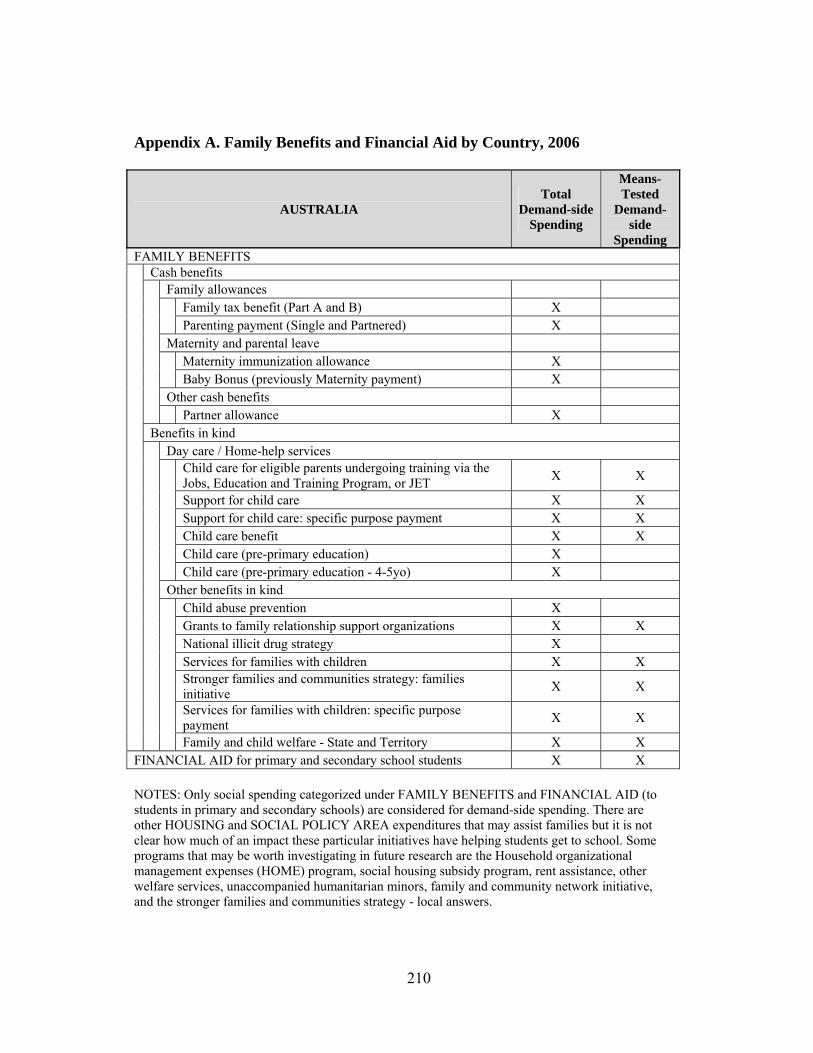
210

Appendix A. Family Benefits and Financial Aid by Country, 2006

AUSTRALIA Total

Demand-side Spending

Means-Tested

Demand-side

Spending FAMILY BENEFITS

Cash benefits

Family allowances

Family tax benefit (Part A and B) X Parenting payment (Single and Partnered) X

Maternity and parental leave

Maternity immunization allowance X Baby Bonus (previously Maternity payment) X

Other cash benefits Partner allowance X

Benefits in kind

Day care / Home-help services

Child care for eligible parents undergoing training via the Jobs, Education and Training Program, or JET

X X

Support for child care X X Support for child care: specific purpose payment X X Child care benefit X X Child care (pre-primary education) X Child care (pre-primary education - 4-5yo) X

Other benefits in kind

Child abuse prevention X Grants to family relationship support organizations X X National illicit drug strategy X Services for families with children X X Stronger families and communities strategy: families initiative

X X

Services for families with children: specific purpose payment

X X

Family and child welfare - State and Territory X X FINANCIAL AID for primary and secondary school students X X

NOTES: Only social spending categorized under FAMILY BENEFITS and FINANCIAL AID (to students in primary and secondary schools) are considered for demand-side spending. There are other HOUSING and SOCIAL POLICY AREA expenditures that may assist families but it is not clear how much of an impact these particular initiatives have helping students get to school. Some programs that may be worth investigating in future research are the Household organizational management expenses (HOME) program, social housing subsidy program, rent assistance, other welfare services, unaccompanied humanitarian minors, family and community network initiative, and the stronger families and communities strategy - local answers.

211

Appendix A, continued

AUSTRIA

Total Demand-

side Spending

Means-Tested Demand-side

Spending

FAMILY BENEFITS


Child benefit (tax system) X Child benefit (Öffenliche Hand) X Child benefit (Sozialleistungen der Länder) X Alimony supplements (Familienlastenausgleichsfonds) X Family support (egalitarian benefits) X Family allowance (Länder) (non means-tested) X

Maternity and parental leave Maternity/parental leave benefit X

Maternity/parental leave benefit (means-tested) X X Aid at child birth X Parental leave (Familien-lastenaus-gleichsfonds) X

Other cash benefits Other benefits in cash (Familienlastenausgleichsfonds) X

Other benefits in cash (Länder) X Other cash lump sum benefits X

Benefits in kind Day care / Home-help services X

Child day care (Kindergarten) X Child day care (Kindergarten) (Sozialleis-tungen der Länder) X Child day care (pre-primary - adjustment for 6yo) X Family accommodation benefits (Sozialleistungen der Länder) X Accommodation benefits (means-tested) X X Home help X Home help (means-tested) X X

Other benefits in kind Other benefits in kind (Sozialleistungen der Länder) X

Family support (Familienlastenausgleichsfonds) X Other benefits in kind (non means-tested) X Other benefits in kind (means-tested) X X

FINANCIAL AID for primary and secondary students X X

NOTES: Only social spending categorized under FAMILY BENEFITS and FINANCIAL AID (to students in primary and secondary schools) are considered for demand-side spending. There are other HOUSING and SOCIAL POLICY AREA expenditures that may assist families but it is not clear how much of an impact these particular initiatives have helping students get to school. Some programs that may be worth investigating in future research are the rent subsidy (Wohnbeihilfen)s, other cash lump sum benefits (Länder means-tested), accommodation (Länder means-tested and non means-tested), and other benefits in kind (Sozialleis-tungen der Gemeinden means-tested).

212


BELGIUM Total Demand-side Spending


Spending

FAMILY BENEFITS Cash benefits

Family allowances National office for employees' family allowances X

Self-employed persons (INASTI) X Employees of public enterprises X National social security office for provincial and local government X Employees of local government enterprises X Employees of hospital welfare centres (CPAS) X Employees of Belgocontrol X Postal services employees (PTT-La Poste) X Civil servants and comparable categories, military and police members X Overseas social security office X Family allowances (means-tested) X X

Maternity and parental leave Parental leave: employees of local government enterprises X

Other parental leave X Maintenance income: employed persons (INAMI & INASTI) X Income maintenance: civil servants and comparable categories, military and police members X Birth grant: National office for employees' family allowances X Birth grant: self-employed persons (INASTI) X Birth grant: employees of public enterprises X Birth grant: National social security office for provincial and local government X Birth grant: Postal services employees (PTT-La Poste) X Birth grant: assistance to welfare centres (CPAS) X X Birth grant: civil servants and comparable categories, military and police members X

213


BELGIUM, continued Total Demand-side

Spending


Spending

Birth grant (not means-tested) X Birth grant (means-tested) X X

Other cash benefits Other cash periodic benefits X


Home-help services X Child day care: all residents X Child care (pre-primary education) X Accommodation: all residents X Home-help: private-sector employees X

Other benefits in kind Other benefits in kind: assistance to welfare centres (CPAS) and others X X Other benefits in kind (not means-tested) X Other benefits in kind: Belgian Railways employees (SNCB) X Other benefits in kind: private-sector employees (pension provision) X

FINANCIAL AID for primary and secondary students X X NOTES: Only social spending categorized under FAMILY BENEFITS and FINANCIAL AID (to students in primary and secondary schools) are considered for demand-side spending. There are other HOUSING and SOCIAL POLICY AREA expenditures that may assist families but it is not clear how much of an impact these particular initiatives have helping students get to school. Some programs that may be worth investigating in future research are: Social housing and Other cash benefits: Income Maintenance, assistance to welfare centres (CPAS).

214


BRAZIL Total Demand-side Spending


Spending

FAMILY BENEFITS Cash Benefits

Bolsa Familia X X Benefits in Kind Social Assistance X X

FINANCIAL AID to students in primary and secondary school X X

NOTES: Only social spending categorized under FAMILY BENEFITS and FINANCIAL AID (to students in primary and secondary schools) are considered for demand-side spending. The OECD's SOCX database did not contain data for family benefits in Brazil because data are not centralized (municipalities bear most of the fiscal responsibility for social programs). Data for the Conditional Cash Transfer program, Bolsa Familia, as well as social assistance spending (the Social Assistance Reference Centres or CRAS and the Comprehensive Family Care Programme or PAIF) were available from Soares 2012, Soares et al. 2010, and Lindert et al. 2007. Other major social assistance programs available in Brazil that are not family-focused include the Continuous Cash Benefit (BPC) which targets the disabled and the elderly (anyone 65 or older) and the General Social Security Regime (RGPS) that employers and employees pay into.

215


CANADA Total Demand-side

Spending Means-Tested



Family allowances Canada Child Tax Benefit X Maternity and parental leave Related family benefits (Parental) (EI) X

Related family benefits (Compassionate Care) (EI) X Québec maternity and parental leave program X


Provincial/territorial regulated childcare allocation X X FINANCIAL AID for primary and secondary students N/A N/A

NOTES: Only social spending categorized under FAMILY BENEFITS and FINANCIAL AID (to students in primary and secondary schools) are considered for demand-side spending. There are other HOUSING and SOCIAL POLICY AREA expenditures that may assist families but it is not clear how much of an impact these particular initiatives have helping students get to school. Some programs that may be worth investigating in future research are housing programs, provincial welfare programs, and net municipal welfare. Canada also does not offer financial aid for primary and secondary students.

216


CHILE Total Demand-side

Spending Means-Tested



Family allowances Family allocations (tax benefits) X

Extraordinary Bonds X Life Insurance X Family subsidies X X Chile Solidario (CCT Program) X X

Maternity and parental leave Maternal Subsidies X


Child day-care: Pre-school education X


NOTES: Only social spending categorized under FAMILY BENEFITS and FINANCIAL AID (to students in primary and secondary schools) are considered for demand-side spending. There are other HOUSING and SOCIAL POLICY AREA expenditures that may assist families but it is not clear how much of an impact these particular initiatives have helping students get to school. Chile has seen a marked decrease in poverty and has increased social spending on housing and other social welfare initiatives but these data were not available for 2006. The data for Chile Solidario comes from three sources: Guardia et al. 2011, Fiszbein and Schady 2009, and the OECD publication “Maintaining Momentum: OECD Perspectives on Policy Challenges in Chile” (OECD 2011d).

217


CZECH REPUBLIC Total



Spending


Family allowances All residents: children's allowance (income based) X X Maternity and parental leave Child-birth grant X

Parental allowance X Income maintenance in the event of childbirth: employed X Income maintenance in the event of childbirth: self employed X Income maintenance in the event of childbirth X

Other cash benefits Social allowance X X

State social benefits Other cash benefits (Employer’s contributions) Other cash benefits (non means-tested) Other cash benefits (means-tested) X X


Child day care (regions/municipalities) X Child care (pre-primary education) X Child day care (pre-primary - adjustment for 6yo) X Accommodation X

FINANCIAL AID to students in primary and secondary school X X NOTES: Only social spending categorized under FAMILY BENEFITS and FINANCIAL AID (to students in primary and secondary schools) are considered for demand-side spending. There are other HOUSING and SOCIAL POLICY AREA expenditures that may assist families but it is not clear how much of an impact these particular initiatives have helping students get to school. Some programs that may be worth investigating in future research are the housing allowance and income maintenance social assistance.

218


DENMARK Total



Spending FAMILY BENEFITS Cash benefits

Family allowances Child family benefit X

Child maintenance benefit paid in advance X X Maternity and parental leave Income maintenance benefit in the event of childbirth X

Parental leave benefits X Benefits in kind Day care / Home-help services

Institutions and family care X Child day care X Child day care (adjustment for 6yo) X Home help for families X

Other benefits in kind Other benefits in kind X


NOTES: Only social spending categorized under FAMILY BENEFITS and FINANCIAL AID (to students in primary and secondary schools) are considered for demand-side spending. There are other HOUSING and SOCIAL POLICY AREA expenditures that may assist families but it is not clear how much of an impact these particular initiatives have helping students get to school. Some programs that may be worth investigating in future research include: Social housing benefits and benefits in kind - social assistance family allowances accommodation.

219


ESTONIA Total




Family allowances Family allowance (non means tested) (Social Insurance

Board) X

Maternity and parental leave Income maintenance (Social Insurance Board) X X

Parental leave (Social Insurance Board) - income based but has a base amount for parents who were unemployed the year preceding the child's birth

X

Birth grant (Social Insurance Board) X Other cash benefits Other cash periodic benefits (non means tested) (State) X

Other cash lump sum benefits (Social Insurance Board) X X Benefits in kind Day care / Home-help services

Accommodation (non means tested) (Ministry of Social Affairs)

X

Child day care (adjustment for 6yo) X Child care (pre-primary education) X

Other benefits in kind Other benefits in kind (non means-tested) - in 2007 this is

split between the Social Insurance Board and the Ministry of Social Affairs. In 2006 these are combined.

X

FINANCIAL AID to students in primary and secondary school X X NOTES: Only social spending categorized under FAMILY BENEFITS and FINANCIAL AID (to students in primary and secondary schools) are considered for demand-side spending. There are other HOUSING and SOCIAL POLICY AREA expenditures that are means-tested and may assist families but it is not clear how much of an impact these particular initiatives have helping students get to school. The means-tested benefits that may be worth investigating in future research include social housing and rent benefits, and income support cash benefits from the Ministry of Social Affairs.

220


FINLAND Total




Family allowances Child allowance X Maternity and parental leave Maternity grant (maternity benefit) X

Parental leave benefit non means-tested (Child home care allowance)

X

Parental leave benefit (Municipal supplements to child day care subsidies)

X X

Other cash benefits Maintenance support (health care and social services) X

Other cash benefits (Sickness insurance) X Benefits in kind Day care / Home-help services

Child day care (Services provided by municipalities) (non means-tested)

X

Child day care (Services provided by municipalities) (means-tested)

X X

Child day care (Municipal supplements to child day care subsidies)

X X

Help at home X Other benefits in kind Institutional care of children and youth X

Other benefits in kind (health care and social services) X Other benefits in kind (The Slot Machine Association) X Parental leave benefit means-tested (Child home care allowance)

X X

Income maintenance (Sickness insurance) X FINANCIAL AID to primary and secondary students X X NOTES: Only social spending categorized under FAMILY BENEFITS and FINANCIAL AID (to students in primary and secondary schools) are considered for demand-side spending. There are other HOUSING and SOCIAL POLICY AREA expenditures that are means-tested and may assist families but it is not clear how much of an impact these particular initiatives have helping students get to school. The benefits that may be worth investigating in future research include housing allowances, income support, and special support provided by the state in the form of benefits in kind or cash benefits.

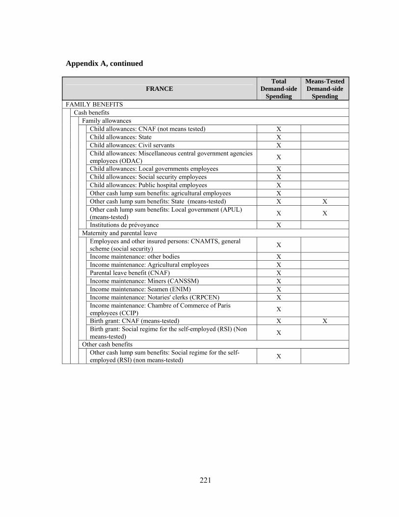
221


FRANCE Total




Family allowances Child allowances: CNAF (not means tested) X

Child allowances: State X Child allowances: Civil servants X Child allowances: Miscellaneous central government agencies employees (ODAC)

X

Child allowances: Local governments employees X Child allowances: Social security employees X Child allowances: Public hospital employees X Other cash lump sum benefits: agricultural employees X Other cash lump sum benefits: State (means-tested) X X Other cash lump sum benefits: Local government (APUL) (means-tested)

X X

Institutions de prévoyance X Maternity and parental leave Employees and other insured persons: CNAMTS, general

scheme (social security) X

Income maintenance: other bodies X Income maintenance: Agricultural employees X Parental leave benefit (CNAF) X Income maintenance: Miners (CANSSM) X Income maintenance: Seamen (ENIM) X Income maintenance: Notaries' clerks (CRPCEN) X Income maintenance: Chambre of Commerce of Paris employees (CCIP)

X

Birth grant: CNAF (means-tested) X X Birth grant: Social regime for the self-employed (RSI) (Non means-tested)

X

Other cash benefits Other cash lump sum benefits: Social regime for the self-

employed (RSI) (non means-tested) X

222


FRANCE, continued Total



Spending

Benefits in kind

Benefits in kind


Child care: CNAF (means tested) X X Child care: CRPEN (means tested) X X Child care: State (means-tested) X X Child care: Local government (APUL) (means-tested) X X Pre-primary education X Child care: Civil servants (means tested) X X Child care: National Family Allowances Fund Caisse (Caisse Nationale des Allocations Familiales (CNAF))

X

Home help: CNAF (means-tested) X X Home help: Caisse nationale militaire de sécurité sociale (CNMSS)

X

Home help: Local government (APUL) X Home help: Notaries' clerks (CRPCEN) X

Other benefits in kind Other benefits in kind: Caisse nationale militaire de sécurité

sociale (CNMSS) (means-tested) X X

Other benefits in kind: Local government employees (CNRACL)

X

Other benefits in kind: ARRCO X Other benefits in kind: State (non means-tested) X Other benefits in kind: Local government (APUL) (non means-tested)

X


NOTES: Only social spending categorized under FAMILY BENEFITS and FINANCIAL AID (to students in primary and secondary schools) are considered for demand-side spending. There may be other HOUSING and SOCIAL POLICY AREA expenditures that may assist families but it is not clear if such initiatives impact helping students get to school.

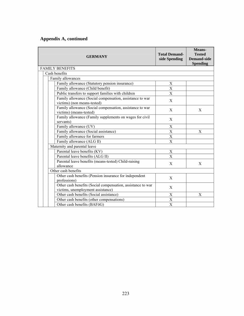
223


GERMANY Total Demand-side Spending

Means-Tested



Family allowances Family allowance (Statutory pension insurance) X

Family allowance (Child benefit) X Public transfers to support families with children X Family allowance (Social compensation, assistance to war victims) (non means-tested)

X

Family allowance (Social compensation, assistance to war victims) (means-tested)

X X

Family allowance (Family supplements on wages for civil servants)

X

Family allowance (UV) X Family allowance (Social assistance) X X Family allowance for farmers X Family allowance (ALG II) X

Maternity and parental leave Parental leave benefits (KV) X

Parental leave benefits (ALG II) X Parental leave benefits (means-tested) Child-raising allowance

X X

Other cash benefits Other cash benefits (Pension insurance for independent

professions) X

Other cash benefits (Social compensation, assistance to war victims, unemployment assistance)

X

Other cash benefits (Social assistance) X X Other cash benefits (other compensations) X Other cash benefits (BAFöG) X

224


GERMANY, continued Total Demand-side Spending

Means-Tested



Child day care (Youth assistance) X Child day care (pre-primary - adjustment for 6yo) X

Other benefits in kind Youth assistance X

Social assistance X X FINANCIAL AID to students in primary and secondary school X X NOTES: Only social spending categorized under FAMILY BENEFITS and FINANCIAL AID (to students in primary and secondary schools) are considered for demand-side spending. There are other HOUSING and SOCIAL POLICY AREA expenditures that are means-tested and may assist families but it is not clear if such initiatives impact helping students get to school. Benefits that may be worth investigating in future research include housing assistance cash benefits, income support social assistance, and other social assistance cash benefits and benefits in kind.

225


HUNGARY

Total Demand-

side Spending

Means-Tested



Family allowances Family or child allowance (non means-tested) X

Family or child allowance (means-tested) X X Birth grant (non means-tested) X

Maternity and parental leave Income maintenance in the event of childbirth (non means-tested) X

Parental leave benefit (non means-tested) X Other cash benefits Other cash periodic benefits (means-tested) X X

Other cash lump sum benefits (means-tested) X X Other cash periodic benefits (GYV-GYJO) X Other cash lump sum benefits (non means-tested) X


Child day care (non means-tested) X Child care (pre-primary education) X Other benefits in kind Accommodation (non means-tested) X Other benefits in kind (non means-tested) X Other benefits in kind (means-tested) X X


NOTES: Only social spending categorized under FAMILY BENEFITS and FINANCIAL AID (to students in primary and secondary schools) are considered for demand-side spending. There are other HOUSING and SOCIAL POLICY AREA expenditures that are means-tested and may assist families but it is not clear how much of an impact these particular initiatives have helping students get to school. Benefits that are means-tested and may be worth investigating in future research include housing assistance (rent benefits and benefits to owner-occupiers), income maintenance/income support, other cash periodic benefits, cash lump sum benefits, and other means-tested benefits in kind.

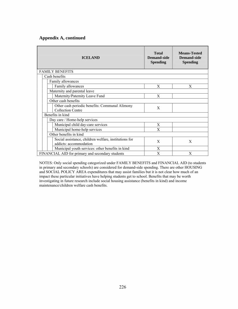
226


ICELAND Total



Spending


Family allowances Family allowances X X Maternity and parental leave Maternity/Paternity Leave Fund X Other cash benefits Other cash periodic benefits: Communal Alimony

Collection Centre X


Municipal child day-care services X Municipal home-help services X

Other benefits in kind Social assistance, children welfare, institutions for

addicts: accommodation X X

Municipal youth services: other benefits in kind X FINANCIAL AID for primary and secondary students X X

NOTES: Only social spending categorized under FAMILY BENEFITS and FINANCIAL AID (to students in primary and secondary schools) are considered for demand-side spending. There are other HOUSING and SOCIAL POLICY AREA expenditures that may assist families but it is not clear how much of an impact these particular initiatives have helping students get to school. Benefits that may be worth investigating in future research include social housing assistance (benefits in kind) and income maintenance/children welfare cash benefits.

227


IRELAND Total




Family allowances All residents: standard child benefit X

Children's allowance for civil servants: teachers, army X Family allowance (non-contributory) X Family allowance (social insurance fund) X All residents: family income supplement X X

Maternity and parental leave Employees: maternity benefits (social security) (3) X

Income maintenance (Health benefits) X Other cash benefits Deserted wives' allowance X

All residents: lone parent's allowance X Cash benefits by Health services X Other cash benefits: employees X X


Child care (pre-primary education) X Accommodation X Home help X

Other benefits in kind Family allowances through national health services X


NOTES: Only social spending categorized under FAMILY BENEFITS and FINANCIAL AID (to students in primary and secondary schools) are considered for demand-side spending. There are other HOUSING and SOCIAL POLICY AREA expenditures that may assist families but it is not clear how much of an impact these particular initiatives have helping students get to school. Benefits that may be worth investigating in future research include social housing assistance (benefits in kind) and income maintenance/children welfare cash benefits.

228


ISRAEL Total




Family allowances Child allowance (NII) X

Study grant (NII) - to help school-age children buy school equipment (means-tested)

X X

Alimony (NII) X Maternity and parental leave Maternity allowance and vacation pay (NII) X Other cash benefits Cash benefits for needy families X X

Birth grant (NII) X Benefits in kind Day care / Home-help services

Local authorities day care programs X Child care programs (NPIs) X Pre-primary educational institutions X

Other benefits in kind Child and family welfare services X X

Rehabilitation programs for youth X X FINANCIAL AID for primary and secondary students X X NOTES: Only social spending categorized under FAMILY BENEFITS and FINANCIAL AID (to students in primary and secondary schools) are considered for demand-side spending. There are other HOUSING and SOCIAL POLICY AREA expenditures that may assist families but it is not clear how much of an impact these particular initiatives have helping students get to school. Benefits that may be worth investigating in future research include housing assistance, cash benefits for the socially excluded and needy, the earned income tax credit, assistance to the socially excluded and new immigrants, food provisions to the needy, philanthropy funds, and subsidized public transportation.

229


ITALY Total Demand-side Spending



Family allowances Family or child allowances (means-tested) X X

Family or child allowances (means-tested): Employees' temporary benefits [managed by INPS]

X X

Family or child allowances (means-tested): Social Security Funds for professional categories

X X

Family or child allowances (means-tested): Occupational Injury Insurance [managed by INAIL]

X X

Maternity and parental leave Income in the event of childbirth (non means-tested) X

Income in the event of childbirth (means-tested) X X Other cash benefits Other cash periodic benefits (means-tested) X X


Child care (pre-primary education) X Child day care X

Other benefits in kind Other benefits in kind for family (non means-tested) X

Other benefits in kind for family (means-tested) X X Accommodation for family


NOTES: Only social spending categorized under FAMILY BENEFITS and FINANCIAL AID (to students in primary and secondary schools) are considered for demand-side spending. There are other HOUSING and SOCIAL POLICY AREA expenditures that may assist families but it is not clear how much of an impact these particular initiatives have helping students get to school. Benefits that may be worth investigating in future research include housing assistance and income maintenance, as well as mandatory private cash benefits such as the means-tested compulsory occupational social insurance that is managed by public sector employers.

230


JAPAN Total




Family allowances Children's allowances X

Rearing allowances for handicapped children X Allowances for children in lone parents' family X

Maternity and parental leave Maternity allowance: Japan Health Insurance Association X

Maternity allowance: society managed health insurance X Maternity allowance: National health insurance X Maternity allowance: seamen's insurance X Maternity allowance: Promotion and Mutual Aid corporation for Private Schools of Japan (Former Mutual aid association of private school personnel)

X

Maternity allowance: National public service mutual aid association

X

Maternity allowance: local public employees' mutual aid association

X

Maternity allowance: unemployment insurance X Other cash benefits Local public employees' mutual aid association X


Children's allowances X Social welfare (subsidies for children's protection) X X Child care (pre-primary education) X

Other benefits in kind Children's allowances (other) X

Social welfare (subsidies for children's protection, other) X X FINANCIAL AID for primary and secondary students X X

NOTES: Only social spending categorized under FAMILY BENEFITS and FINANCIAL AID (to students in primary and secondary schools) are considered for demand-side spending. There are other HOUSING and SOCIAL POLICY AREA expenditures that may assist families but it is not clear how much of an impact these particular initiatives have helping students get to school. Benefits that may be worth investigating in future research include income maintenance cash benefits for public assistance and social welfare.

231


KOREA Total Demand-side Spending



Family allowances Lone parent families X

Patriots and veteran pension, etc. X Maternity and parental leave Prenatal and postnatal leave allowances (Employment

Insurance) X

Maternity leave allowances (Employment Insurance) X Benefits in kind Day care / Home-help services

Day care for child & adolescent X Pre-school education only X Child care (pre-primary education) X Support for day care for family X X

Other benefits in kind Welfare centers X X

Children facilities X Family welfare X X Residential service for women & families X Sub-other X

FINANCIAL AID for primary and secondary students X X NOES: Only social spending categorized under FAMILY BENEFITS and FINANCIAL AID (to students in primary and secondary schools) are considered for demand-side spending. There are other HOUSING and SOCIAL POLICY AREA expenditures that may assist families but it is not clear how much of an impact these particular initiatives have helping students get to school. Benefits that may be worth investigating in future research include food bank social assistance, price reductions for low-income families, and public housing costs for low-income families. Mandatory private benefits-in-kind that may have an impact on students in particular is the transportation and telecommunication fee reduction (for children).

232


MEXICO Total



Spending


Other cash benefits Education, health and feeding national program:

PROGRESA/Oportunidades (SEDESOL, The Ministry of Social Development)

X X

Nutritional Support Program (SEDESOL) X X Benefits in kind Day care / Home-help services

Child day care institutions (ISSSTE, Social and Security Services for State Workers) X X

Child day care institutions (IMSS, Mexican Social Healthcare Institute) X X

Child care (pre-primary education) X Home-help services to children (abandoned or abused children, DIF) X X

Other benefits in kind Food to families program (DIF) X X

Food program school breakfast (DIF) X X Social milk program (SEDESOL) X X Sports promotion (ISSSTE) X X Rural Supply Program (SEDESOL-DICONSA) X X

FINANCIAL AID for primary and secondary students X X NOTES: Only social spending categorized under FAMILY BENEFITS and FINANCIAL AID (to students in primary and secondary schools) are considered for demand-side spending. Nearly all of Mexico's programs target the poor given the rate of poverty in the country. The World Bank estimates that about 43% of the Mexican population lived at or below the poverty line in 2006 (World Bank 2012a). The only benefit not considered means-tested is the pre-primary education child care since it is available to everyone. Yet, since most wealthy families opt to sent their children to private schools, even this benefit is really more of a help to poor families. There are other HOUSING and SOCIAL POLICY AREA expenditures that may also assist poor families but it is not clear how much of an impact these particular initiatives have helping students get to school. Benefits that may be worth investigating in future research include the rural housing program and worthy housing initiative sponsored by the Ministry of Social Development or SEDESOL, as well as the social housing credit provided by the National Trust fund for Popular Housing or FONHAPO.

233


NETHERLANDS

Total Demand-

side Spending


Spending


Family allowances All residents: child allowance X Maternity and parental leave X Other cash benefits Other periodic cash benefits X


All residents: family help and care, home help financed through AWBZ X

Child care (pre-primary education) X Child day care (non means-tested) X

FINANCIAL AID for primary and secondary students X X NOTES: Only social spending categorized under FAMILY BENEFITS and FINANCIAL AID (to students in primary and secondary schools) are considered for demand-side spending. Starting in 2008 a means-tested child allowance cash benefit was introduced. Only 2006 benefits are listed here though the means-tested benefit is included for the 2006-2009 EPI averages. There are other HOUSING and SOCIAL POLICY AREA expenditures that may also help families but it is not clear how much of an impact these particular initiatives have helping students get to school. Benefits that may be worth investigating in future research include social provisions to the poor.

234


NEW ZEALAND Total Demand-side Spending


Spending FAMILY BENEFITS

Cash benefits

Family allowances

Family (Support) Tax Credit X X Child Tax Credit X X Parental Tax Credit X In Work Payment X

Minimum Family Tax Credit X

Maternity and parental leave Maternity and parental leave X Other cash benefits Domestic Purposes Benefit for sole parents X

Benefits in kind


Childcare Assistance X X Out of school care and recreation (OSCAR) X Early Childhood Education Subsidies X X Early Childhood Education Grants X X Child care (pre-primary education: 5 years old) X

Other benefits in kind

Commissioner for children X Education and prevention services X X Family wellbeing services X X Counseling and rehabilitation services X Families Commission X

FINANCIAL AID for primary and secondary students X X NOTES: Only social spending categorized under FAMILY BENEFITS and FINANCIAL AID (to students in primary and secondary schools) are considered for demand-side spending. There are other HOUSING and SOCIAL POLICY AREA expenditures that may also assist families but it is not clear how much of an impact these particular initiatives have helping students get to school. Benefits that may be worth investigating in future research include housing assistance, community housing rental subsidies, strong families benefits in kind, and the youth development partnership fund.

235


NORWAY Total




Family allowances Family allowances for children X Maternity and parental leave Maternity and parental leave benefits X

Income maintenance in the event of childbirth X Birth grant X

Other cash benefits Lone parent cash benefit X


Child day care institutions X Other benefits in kind Accommodation X X

Other benefits in kind X X Home help X

FINANCIAL AID for primary and secondary students X X NOTES: Only social spending categorized under FAMILY BENEFITS and FINANCIAL AID (to students in primary and secondary schools) are considered for demand-side spending. There are other HOUSING and SOCIAL POLICY AREA expenditures that may also assist families but it is not clear how much of an impact these particular initiatives have helping students get to school. Benefits that may be worth investigating in future research include means-tested income support cash benefits, as well as social assistance and means-tested accommodation benefits in kind.

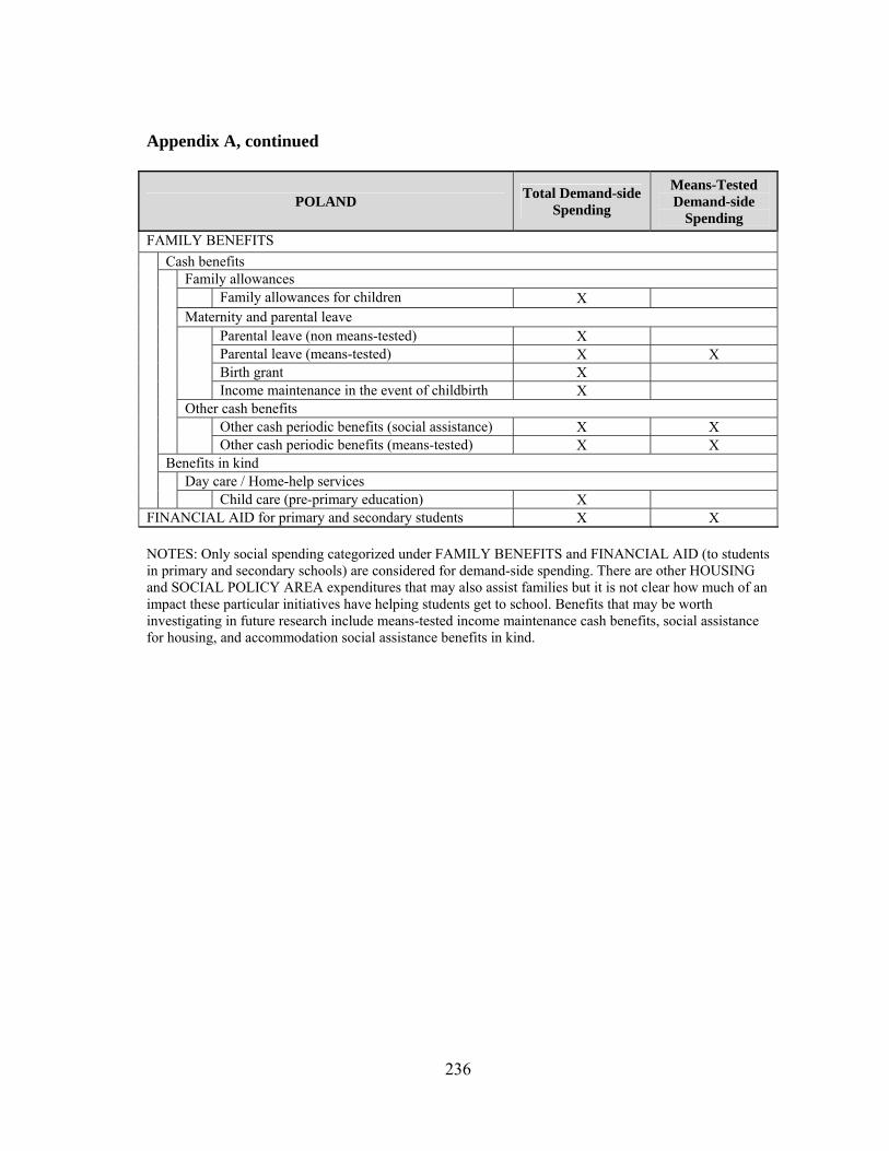
236


POLAND Total Demand-side

Spending


Spending

FAMILY BENEFITS


Family allowances for children X Maternity and parental leave

Parental leave (non means-tested) X Parental leave (means-tested) X X Birth grant X Income maintenance in the event of childbirth X

Other cash benefits Other cash periodic benefits (social assistance) X X

Other cash periodic benefits (means-tested) X X Benefits in kind Day care / Home-help services

Child care (pre-primary education) X FINANCIAL AID for primary and secondary students X X NOTES: Only social spending categorized under FAMILY BENEFITS and FINANCIAL AID (to students in primary and secondary schools) are considered for demand-side spending. There are other HOUSING and SOCIAL POLICY AREA expenditures that may also assist families but it is not clear how much of an impact these particular initiatives have helping students get to school. Benefits that may be worth investigating in future research include means-tested income maintenance cash benefits, social assistance for housing, and accommodation social assistance benefits in kind.

237


PORTUGAL Total


Means-Tested



Family allowances Benefits managed by the central administration X

Benefits managed by the local administration X Child allowance (CGA) X Social Security Subsystem for family protection X X Social Security Subsystem for solidarity (means-tested) X X Social services (public sector) (means-tested) X X General retirement fund (civil servants, pensioners) X

Maternity and parental leave Benefits managed by the central administration X

Social Security Subsystem: income maintenance X Social Security Subsystem for solidarity: income maintenance

X X

Central administration X Other cash benefits Social Security Subsystem for family protection X

Social Security Subsystem for solidarity X Social Security Subsystem for solidarity (means-tested) X X Benefits managed by the central administration: other cash periodic benefits

X

Benefits managed by the local administration: other cash periodic benefits

X

CGA: other cash periodic benefits X Social services (public sector): other cash periodic benefits (non means-tested)

X

Social services (public sector): other cash periodic benefits (means-tested)

X X

General retirement fund (civil servants, pensioners): other cash periodic benefits

X

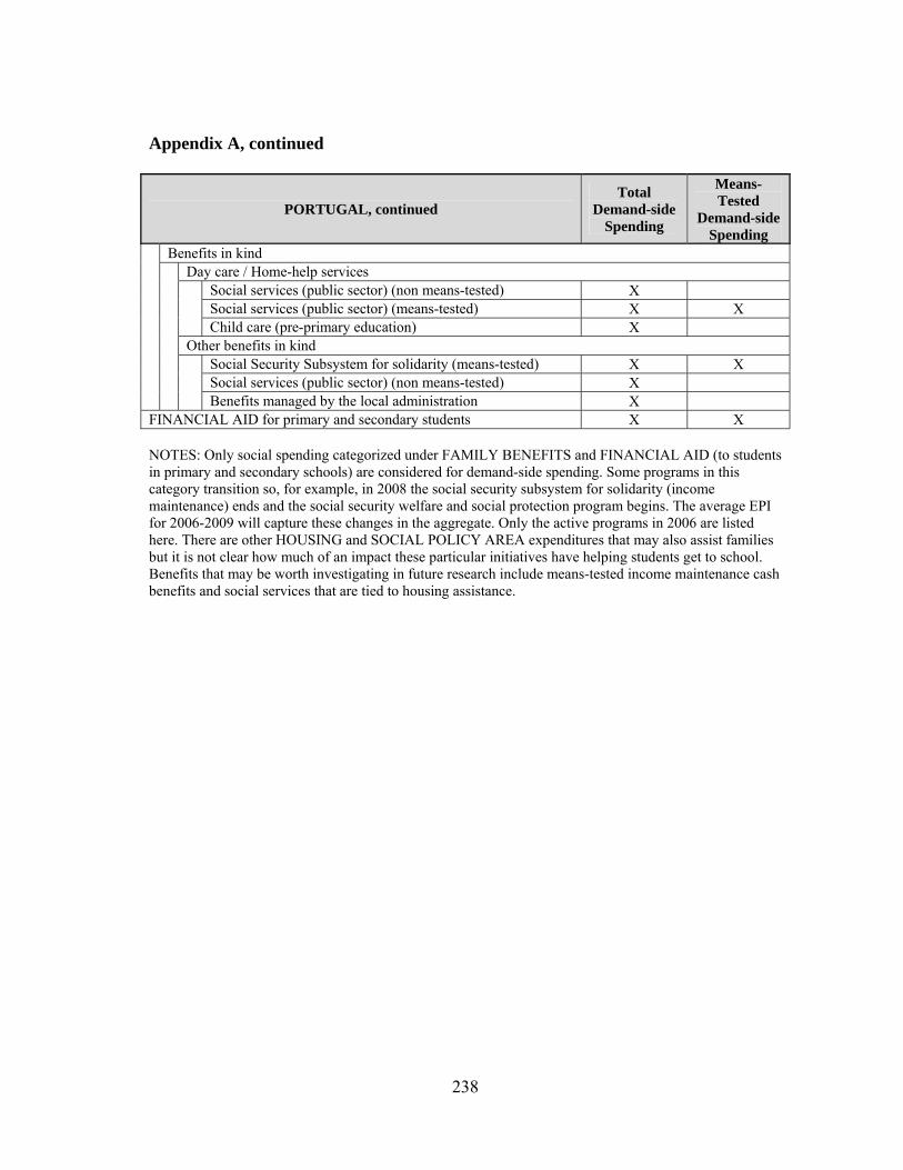
238


PORTUGAL, continued Total


Means-Tested



Social services (public sector) (non means-tested) X Social services (public sector) (means-tested) X X Child care (pre-primary education) X

Other benefits in kind Social Security Subsystem for solidarity (means-tested) X X

Social services (public sector) (non means-tested) X Benefits managed by the local administration X

FINANCIAL AID for primary and secondary students X X NOTES: Only social spending categorized under FAMILY BENEFITS and FINANCIAL AID (to students in primary and secondary schools) are considered for demand-side spending. Some programs in this category transition so, for example, in 2008 the social security subsystem for solidarity (income maintenance) ends and the social security welfare and social protection program begins. The average EPI for 2006-2009 will capture these changes in the aggregate. Only the active programs in 2006 are listed here. There are other HOUSING and SOCIAL POLICY AREA expenditures that may also assist families but it is not clear how much of an impact these particular initiatives have helping students get to school. Benefits that may be worth investigating in future research include means-tested income maintenance cash benefits and social services that are tied to housing assistance.

239


SLOVAK REPUBLIC Total




Family allowances Birth grant (non means-tested) X Family allowances (non means-tested) X Maternity and parental leave Financial assistance in maternity (non means-tested) X Parental leave benefits (non means-tested) X Other cash benefits Other cash periodic benefits X X Other cash sickness lump sum benefits (non means-tested) X


Children's homes (non means-tested) X Child care (pre-primary education) X

FINANCIAL AID for primary and secondary students X X NOTES: Only social spending categorized under FAMILY BENEFITS and FINANCIAL AID (to students in primary and secondary schools) are considered for demand-side spending. Means-tested children allowances were introduced in 2009 along with child day care state social support and other state social support. These additions are accounted for in the average EPI scores but only the benefits paid out in 2006 are listed here. There are other HOUSING and SOCIAL POLICY AREA expenditures that may also assist families but it is not clear how much of an impact these particular initiatives have helping students get to school. Benefits that may be worth investigating in future research include means-tested social help cash benefits intended for income maintenance and accommodation benefits in kind, as well as mandatory private family benefits in kind.

240


SLOVENIA

Total Demand-

side Spending

Means-Tested

Demand-side


Family allowances Other rights from Family Income Act X Maternity and parental leave Maternity leave compensation X

Parental leave: Maternity leave compensation X Parental leave: Other rights from Family Income Act X

Other cash benefits Other cash periodic benefits: Other rights from Family Income Act X

Other cash lump sum benefits: Other rights from Family Income Act X Benefits in kind Day care / Home-help services

Accommodation: Social welfare X X Child day-care: Pre-school education X

Other benefits in kind Other rights from Family Income Act X

FINANCIAL AID for primary and secondary students X X NOTES: Only social spending categorized under FAMILY BENEFITS and FINANCIAL AID (to students in primary and secondary schools) are considered for demand-side spending. In 2007 Slovenia adopted the EURO and in 2009 spending dropped significantly due to the global recession. The family allowance spending data were pulled for this research in April 2012 and confirmation review of the data in February 2013 show changes in these expenditures. The SOCX support team responded to an inquiry and explained that tax credits had been incorporated in the total. The data were updated accordingly. There are other HOUSING and SOCIAL POLICY AREA expenditures that may also assist families but it is not clear how much of an impact these particular initiatives have helping students get to school. Benefits that may be worth investigating in future research include social welfare spending for income maintenance, social assistance, and other benefits in kind.

241


SPAIN Total




Family allowances Family allowance: employees and self-employed (social

security) (non means-tested) X

Family allowance: employees and self-employed (social security) (means-tested)

X X

Family allowance: civil servants, military personnel and local government employees

X

Family allowance: other social protection schemes (non means-tested)

X

Family allowance: companies (non means-tested) X Maternity and parental leave Income maintenance for employees and self-employed

(social security) X

Income maintenance for civil servants, military personnel and local government

X

Income maintenance (companies) X Birth grant: employees and self-employed (social security) X Birth grant: employees and self-employed (social security) (non means-tested)

X

Birth grant: employees and self-employed (social security) (means tested)

X X

Other cash benefits Other cash lump-sum benefits (non means-tested) X

Other periodic benefits for other social protection schemes (means-tested)

X X

242


SPAIN, continued Total



Spending


Day care: other social protection schemes X Day care: companies X Accommodation: other social protection schemes (means-tested)

X X

Accommodation: companies (means-tested) X X Home-help: other social protection schemes (means-tested) X X

Other benefits in kind Other benefits in kind: other social protection schemes (non

means-tested) X

Other benefits in kind: other social protection schemes (means-tested)

X X

Other benefits in kind: other social protection schemes (means-tested)

X X

Other benefits in kind: companies (non means-tested) X FINANCIAL AID for primary and secondary students X X NOTES: Only social spending categorized under FAMILY BENEFITS and FINANCIAL AID (to students in primary and secondary schools) are considered for demand-side spending. There are other HOUSING and SOCIAL POLICY AREA expenditures that may also assist families but it is not clear how much of an impact these particular initiatives have helping students get to school. Benefits that may be worth investigating in future research include housing benefits in kind and cash benefits for income maintenance and support for other social protection schemes, and accommodation for social assistance benefits in kind.

243


SWEDEN

Total Demand-

side Spending


Spending


Family allowances Family or child allowance X Maternity and parental leave Income support during parental leave (operated through

"parental insurance" since 1999) X

Income maintenance (parental insurance) X Adoption allowance X

Other cash benefits Other cash benefits X


Child care X Child day care (adjustment for 6yo) X Child care (pre-primary education) X Accommodation X Child day care (social services bought by local government) X X Accommodation (social services bought by local government) X X Home help X Home help (Privately produced social-services provision) (non means-tested)

X

Other benefits in kind Other benefits in kind X Other benefits in kind (social services bought by local

government) X X

FINANCIAL AID for primary and secondary students X X NOTES: Only social spending categorized under FAMILY BENEFITS and FINANCIAL AID (to students in primary and secondary schools) are considered for demand-side spending. There are other HOUSING and SOCIAL POLICY AREA expenditures that may also assist families but it is not clear how much of an impact these particular initiatives have helping students get to school. Benefits that may be worth investigating in future research include social assistance spending in the areas of income maintenance, accommodation, and other social services.

244


SWITZERLAND Total




Family allowances Family allowances in agricultural sector (not means tested) X

Family allowances in agricultural sector (means tested) X X Family allowances (AF) (cantonal level) X

Maternity and parental leave Maintenance income: salary paid during maternity leave X


Child care: youth protection X X Accommodation: youth protection X X Child care (pre-primary education) X

FINANCIAL AID to students in primary and secondary school X X NOTES: Only social spending categorized under FAMILY and FINANCIAL AID (to students in primary and secondary schools) are considered for demand-side spending. There are other HOUSING and SOCIAL POLICY AREA expenditures that may assist families but it is not clear how much of an impact these particular initiatives have helping students get to school. Some programs that may be worth investigating in future research includes: Social housing benefits, social assistance rent benefits, maintenance income - scholarships and social assistance, other benefits in kind: social assistance.

245


TURKEY Total



Spending


Maternity and parental leave Maternity benefits X

Social Solidarity Fund - SSF - Conditional Cash Transfer X X Benefits in kind Day care / Home-help services

Household services X FINANCIAL AID to students in primary and secondary school X NOTES: Only social spending categorized under FAMILY and FINANCIAL AID (to students in primary and secondary schools) are considered for demand-side spending. Turkey does not provide much social policy expenditure data to the OECD/SOCX database and had included their Conditional Cash Transfer spending (the Social Solidarity Fund or SSF) in FINANCIAL AID. For comparability purposes, this spending was moved to the cash benefits category. There are other POLICY SOCIAL EXPENDITURES (Public cash benefits and public benefits in kind) listed as broad categories and this spending may assist families but it is not clear how much of an impact these initiatives have helping students get to school.

246


UNITED KINGDOM

Total Demand-

side Spending


Spending


Family allowances All residents: child benefit X Maternity and parental leave Employees: statutory maternity pay (SMP) (social security) X

Income maintenance X Other cash benefits Working Tax Credit (cash part, less child care component) X

Child Tax credit (cash part) X Lump sum: income support, family credit and social funds (means-tested) X X

Periodic: income support, family credit and social funds (means-tested) X X


Child care pre primary (3 and 4 years old) X Child care component of FC/WFTC/WTC X X Child care pre primary (adjustment for pre-primary education: 5 years old) X

Family support: local authority personal social services X X Home help: local authority personal social services X X

Other benefits in kind All residents: free school milk and/or meals (non means-tested) X

All residents: free school milk and/or meals (means-tested) X X All residents: Central Government personal social services X X All residents: welfare foods provision X X Accommodation: Local Authority personal social services X X

FINANCIAL AID for primary and secondary students X X NOTES: Only social spending categorized under FAMILY and FINANCIAL AID (to students in primary and secondary schools) are considered for demand-side spending. There are other HOUSING and PUBLIC SOCIAL EXPENDITURES that may also assist families but it is not clear how much of an impact these particular initiatives have helping students get to school. Benefits that may be worth investigating in future research include social housing, benefits in kind, public cash benefits, and public benefits in kind.

247


THE UNITED STATES Total




Family allowances Temporary Assistance for Needy Families (TANF) X X


Child care (pre-primary education) X X Other benefits in kind Child welfare: IV-B programs X X

Child welfare: IV-E (Foster care programs) (Federal) X X Social Service Block Grant (SSBG) X X Child Care Development Block grant (CCDBG) X X Child Support Enforcement (CSE) X Special Supplemental Nutrition Program for Women, Infants and Children (WIC)

X X

Child nutrition and special milk programs X X Commodity donations (CSFP and others) X X

FINANCIAL AID to students in primary and secondary school N/A N/A NOTES: Only social spending categorized under FAMILY and FINANCIAL AID (to students in primary and secondary schools) are considered for demand-side spending. There are other HOUSING and SOCIAL POLICY AREA expenditures that may help families but it is not clear how much of an impact these particular initiatives have helping students get to school. Some programs that may be worth investigating further include: Food stamps, earned income tax credit (refundable part), and the low-income housing energy assistance program.

248

Appendix B. Chapter III Hypotheses and Independent Variables Unpacked

Hypotheses Operationalization

Expected Sign Relative

to the EPI (Dependent Variable)*

Data Source

Hypothesis 3.1: Countries that are considered liberal welfare regimes will allocate more resources to schools (supply-side policies) than to family or student benefits (demand-side policies); conservative regimes will allocate funds a bit more evenly whereas univeralist regimes will devote more resources to demand-side policies.

See Table III-1 for country scores. Each score in the capital welfare typology is between 0 and 12 and is based on a variety of stratification indices. Depending on how the country handles pensions, unemployment, etc., it is given a score that indicates to what degree it falls into each category: liberal, conservative, or social democratic

Liberal (+)

Conservative (+)

Social (-)

The Three Worlds of Welfare

Capitalism, Gøsta Esping-Andersen

(1990) - Table 3.1, 70-1

Hypothesis 3.2: Proportionally Representative (PR) Systems will spend relatively more than majoritarian systems on demand-side policies that are student and family-oriented than on supply-side policies that target schools and teacher wages.

Classification of the electoral system. (1) Majoritarian (2) Combined (mixed) (3) Proportional (PR) _

Quality of Government

database (University of Gothenberg)

Hypothesis 3.3: More democratic countries will invest more in education (supply-side policies) than in family and student benefits (demand-side policies) to assure that citizens are able to participate in the economy as well as the running and monitoring of government.

Each country is scored on its level of political rights and civil liberties. A rating of 1 indicates the highest degree of freedom and 7 the lowest level of freedom. All countries in this dataset are between 1 and 3.

+ Freedom House - Freedom in the World Survey

249

Appendix B, continued

Hypotheses Operationalization

Expected Sign Relative

to the EPI (Dependent Variable)*

Data Source

Hypothesis 3.4: Left-learning governments will spend more on demand-side policies that are student and family-oriented than on supply-side policies that target schools and teacher wages.

Ideology of the largest party in government OR ideology of the executive's party: (1) Right (2) Center (3) Left

_

The World Bank's Database of

Political Institutions

Hypothesis 3.5: When a country has strong unions and a PR (proportionally representative) electoral system, spending on supply-side expenses (schools and wages) would be expected to be higher relative to demand-side spending (expenditures that go directly to students and families).

This is tested with an interaction between the PR measure and the Labor Union Power Index (UP). The UP measures the protection and power of unions on a weighted scale of seven factors that together equal one: (1) Do employees have the right to unionize? (2) Do employees have the right to bargain collectively? (3) Do employees have the legal duty to bargain with unions? (4) Are collective contracts extended to third parties by law? (5) Does the law allow closed shops? (6) Do workers, or unions, or both have a right to appoint members to the Boards of Directors? (7) Are workers’ councils mandated by law?

+**

Quality of Government

database (University of Gothenberg)

* More demand spending means the EPI will be lower (closer to 0) while more supply spending means that the EPI will be higher (closer to 1) **The interaction multiplies two negative numbers together so the coefficient will be positive even though the effect is expected to be negative. This is why the interaction coefficient cannot be directly interpreted and a marginal effect figure is necessary (See Figure 3.5).

250

Appendix C. Elections in 2005 and 2006

Country Legislative Elections Executive Elections

2005 2006 2005 2006

Australia 0 0 0 0 Austria 0 1 0 0 Belgium 0 0 0 0 Brazil 0 1 0 1

Canada 0 1 0 0 Chile 1 0 1 0

Czech Republic 0 1 0 0 Denmark 1 0 0 0 Estonia 0 0 0 1 Finland 0 0 0 1 France 0 0 0 0

Germany 1 0 0 0 Hungary 0 1 1 0 Iceland 0 0 0 0 Ireland 0 0 0 0 Israel 0 1 0 0 Italy 0 1 0 0

Japan 1 0 0 0 S. Korea 0 0 0 0 Mexico 0 0 0 0

Netherlands 0 1 0 1 New Zealand 1 1 0 0

Norway 1 0 0 0 Poland 1 0 1 0

Portugal 1 0 0 0 Slovak Republic 0 1 0 0

Slovenia 0 0 0 0 Spain 0 0 0 0

Sweden 0 1 0 0 Switzerland 0 0 0 0

Turkey 0 0 0 0 UK 1 0 0 0

United States 0 1 0 0

Total 9 12 3 4

251

Appendix D. What’s the difference? Legislative Ideology Versus Executive Ideology

Independent Variables Model 1 Model 2

EPI-A EPI-M EPI-A EPI-M

Executive Ideology -.05 (.03)* -.03 (.03) - - Legislative Ideology - - -.05 (.03)* -.03 (.03)

Electoral System -.24

(.07)** -.04 (.08) -.24 (.07)** -.04 (.08)

Union Power -.94

(.29)** -.04 (.35) -.94 (.29)** -.04 (.35)

Electoral System*Union Power .42 (.13)** .06 (.15) .42 (.13)** .06 (.15) Freedom Index .12 (.07) -.07 (.09) .12 (.07) -.07 (.09) Political Constraint .01 (.27) .06 (.32) .01 (.27) .06 (.32) GDPpc -.00 (.00)* .00 (.00) -.00 (.00) .00 (.00)

Model p-value .03 .71 .03 .71

N=26, Standard errors are in parentheses *p<.10, ** p<.01

252

APPENDIX E. PISA Scores Unpacked

Country School Type

Percent School Type

Percent School Type

(SE)

Reading Mean Score

Reading Mean Score

(SE)

Math Mean Score

Math Mean

Score (SE)

Science Mean Score

Science Mean

Score (SE)

Australia Public 59.72 0.75 497 3.89 499 4.04 511 4.31 Australia Private 40.28 0.75 542 3.01 537 3.05 552 2.67 Australia Other a a a a a a a a Australia All 515 2.30 514 3 527 3 Austria Public 86.76 2.51 465 3.54 493 3.36 491 3.95 Austria Private 12.52 2.4 497 13.68 505 13.11 509 11.9 Austria Other 0.72 0.71 0 0 0 0 0 0 Austria All 470 2.90 496 3 494 3

Belgium Public 30.51 0.65 475 4.08 483 4.22 475 4.44 Belgium Private 69.49 0.65 520 2.93 529 2.71 520 3.18 Belgium Other a a a a a a a a Belgium All 506 2.30 515 2 507 3

Brazil Public 84.91 1.09 398 3.16 373 2.65 393 2.81 Brazil Private 11.86 0.61 516 6.68 485 6.59 505 5.9 Brazil Other 3.23 0.89 381 12.58 355 13.51 379 10.32 Brazil All 412 2.70 386 2 405 2

Canada Public 92.52 0.67 521 1.51 522 1.68 526 1.67 Canada Private 7.48 0.67 566 7.15 582 7.24 567 6.97 Canada Other a a a a a a a a Canada All 524 1.50 527 2 529 2 Chile All 449 3.10 421 3 447 3 Chile Public 40.61 1.61 423 5.17 398 4.66 425 4.45 Chile Private 56.09 2.06 469 3.9 438 4.36 464 3.95 Chile Other 3.3 1.72 452 17.94 417 20.51 439 17.57

Czech Republic Public 95.56 1.2 477 2.99 492 2.95 499 3.21

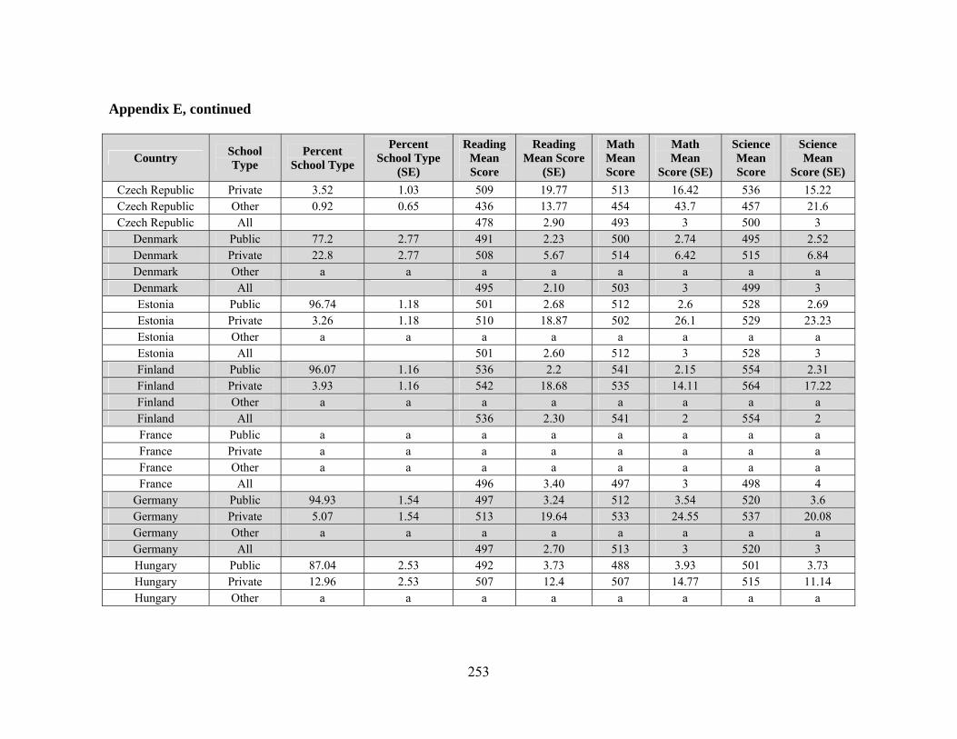
253

Appendix E, continued

Country School Type

Percent School Type

Percent School Type

(SE)

Reading Mean Score

Reading Mean Score

(SE)

Math Mean Score

Math Mean

Score (SE)

Science Mean Score

Science Mean

Score (SE)

Czech Republic Private 3.52 1.03 509 19.77 513 16.42 536 15.22 Czech Republic Other 0.92 0.65 436 13.77 454 43.7 457 21.6 Czech Republic All 478 2.90 493 3 500 3

Denmark Public 77.2 2.77 491 2.23 500 2.74 495 2.52 Denmark Private 22.8 2.77 508 5.67 514 6.42 515 6.84 Denmark Other a a a a a a a a Denmark All 495 2.10 503 3 499 3 Estonia Public 96.74 1.18 501 2.68 512 2.6 528 2.69 Estonia Private 3.26 1.18 510 18.87 502 26.1 529 23.23 Estonia Other a a a a a a a a Estonia All 501 2.60 512 3 528 3 Finland Public 96.07 1.16 536 2.2 541 2.15 554 2.31 Finland Private 3.93 1.16 542 18.68 535 14.11 564 17.22 Finland Other a a a a a a a a Finland All 536 2.30 541 2 554 2 France Public a a a a a a a a France Private a a a a a a a a France Other a a a a a a a a France All 496 3.40 497 3 498 4

Germany Public 94.93 1.54 497 3.24 512 3.54 520 3.6 Germany Private 5.07 1.54 513 19.64 533 24.55 537 20.08 Germany Other a a a a a a a a Germany All 497 2.70 513 3 520 3 Hungary Public 87.04 2.53 492 3.73 488 3.93 501 3.73 Hungary Private 12.96 2.53 507 12.4 507 14.77 515 11.14 Hungary Other a a a a a a a a

254


Country School Type

Percent School Type

Percent School Type

(SE)

Reading Mean Score

Reading Mean Score

(SE)

Math Mean Score

Math Mean

Score (SE)

Science Mean Score

Science Mean

Score (SE)

Hungary All 494 3.20 490 4 503 3 Iceland Public 99.13 0.09 498 1.47 504 1.47 493 1.42 Iceland Private 0.87 0.09 0 0 0 0 0 0 Iceland Other a a a a a a a a Iceland All 500 1.40 507 1 496 1 Ireland Public 38.5 0.39 474 4.93 472 4.34 489 5.65 Ireland Private 61.5 0.39 509 3.69 497 3.07 520 3.89 Ireland Other a a a a a a a a Ireland All 496 3.00 487 3 508 3 Israel All 474 3.60 447 3 455 3 Israel Public 81.61 2.62 470 4.47 443 3.94 451 4.14 Israel Private 17.78 2.56 498 12.97 471 13 478 11.84 Israel Other 0.61 0.56 0 0 0 0 0 0 Italy Public 93.55 0.58 489 1.65 486 2 492 1.9 Italy Private 5.81 0.63 448 8.96 446 7.25 455 8.13 Italy Other 0.64 0.29 385 19.24 406 26.32 401 26.01 Italy All 486 1.60 483 2 489 2 Japan Public 70.7 1.26 522 4 531 3.8 542 3.8 Japan Private 29.3 1.26 514 8.13 525 7.68 533 7.74 Japan Other a a a a a a a a Japan All 520 3.50 529 3 539 3 Korea Public 62.62 4.33 533 5.23 542 6.47 535 5.51 Korea Private 37.38 4.33 549 5.38 554 6.71 544 5.74 Korea Other a a a a a a a a Korea All 539 3.50 546 4 538 3

Mexico Public 88.48 1.14 420 2.09 414 1.86 411 1.82

255


Country School Type

Percent School Type

Percent School Type

(SE)

Reading Mean Score

Reading Mean Score

(SE)

Math Mean Score

Math Mean

Score (SE)

Science Mean Score

Science Mean

Score (SE)

Mexico Private 11.52 1.14 468 4.37 457 5.24 456 4.3 Mexico Other a a a a a a a a Mexico All 425 2.00 419 2 416 2

Netherlands Public 33.96 3.89 515 9.59 531 9.8 526 11.73 Netherlands Private 66.04 3.89 504 8.12 523 7.29 520 7.94 Netherlands Other a a a a a a a a Netherlands All 508 5.10 526 5 522 5

New Zealand Public 94.34 0.43 517 2.31 516 2.36 529 2.57 New Zealand Private 5.66 0.43 586 10.64 580 8.66 588 11.11 New Zealand Other a a a a a a a a New Zealand All 521 2.40 519 2 532 3

Norway Public 98.63 0.43 503 2.57 498 2.42 500 2.61 Norway Private 1.37 0.43 465 26.77 454 23.53 456 20.76 Norway Other a a a a a a a a Norway All 503 2.60 498 2 500 3 Poland Public 97.87 0.1 499 2.66 493 2.86 507 2.46 Poland Private 2.13 0.1 554 11.74 557 11.86 563 10.76 Poland Other a a a a a a a a Poland All 500 2.60 495 3 508 2

Portugal Public 85.53 2.7 485 3.31 482 3.12 489 3.13 Portugal Private 14.47 2.7 516 9.21 514 10.39 516 9.27 Portugal Other a a a a a a a a Portugal All 489 3.10 487 3 493 3

Slovak Republic Public 91.01 2.38 475 3.03 495 3.47 489 3.29 Slovak Republic Private 8.99 2.38 499 14.34 512 15.53 505 12.74 Slovak Republic Other a a a a a a a a

256


Country School Type

Percent School Type

Percent School Type

(SE)

Reading Mean Score

Reading Mean Score

(SE)

Math Mean Score

Math Mean

Score (SE)

Science Mean Score

Science Mean

Score (SE)

Slovak Republic All 477 2.50 497 3 490 3 Slovenia Public 97.34 0.06 481 1.05 499 1.23 509 1.16 Slovenia Private 2.66 0.06 561 6 596 7.25 598 7.27 Slovenia Other a a a a a a a a Slovenia All 483 1.00 501 1 512 1

Spain Public 65.92 0.88 469 2.28 473 2.37 478 2.43 Spain Private 34.08 0.88 505 3.76 504 3.73 509 3.4 Spain Other a a a a a a a a Spain All 481 2.00 483 2 488 2

Sweden Public 89.96 0.82 494 2.84 491 2.88 492 2.71 Sweden Private 10.04 0.82 529 11.08 521 11.43 521 11.47 Sweden Other a a a a a a a a Sweden All 497 2.90 494 3 495 3

Switzerland Public 91.87 2.1 500 2.61 534 3.48 516 2.98 Switzerland Private 6.26 1.57 518 9.63 541 11.67 529 7.94 Switzerland Other 1.86 1.43 443 17.33 492 21.66 480 19.17 Switzerland All 501 2.40 534 3 517 3

Turkey Public 99.21 0.56 464 3.59 444 4.49 453 3.65 Turkey Private 0.79 0.56 546 2.25 571 4.91 545 4.81 Turkey Other a a a a a a a a Turkey All 464 3.50 445 4 454 4

UK Public 93.52 1.09 492 2.54 490 2.74 510 2.81 UK Private 6.31 1.1 553 5.37 546 5.69 583 6.81 UK Other 0.17 0.1 504 11.47 491 4.6 512 3.47 UK All 494 2.30 492 2 514 3

USA Public 91.18 1.37 494 3.35 482 3.55 496 3.41

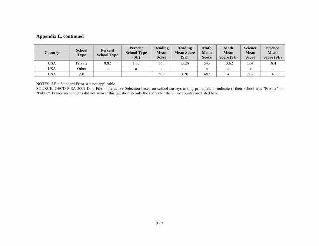
257


Country School Type

Percent School Type

Percent School Type

(SE)

Reading Mean Score

Reading Mean Score

(SE)

Math Mean Score

Math Mean

Score (SE)

Science Mean Score

Science Mean

Score (SE)

USA Private 8.82 1.37 565 15.28 543 13.62 564 18.4 USA Other a a a a a a a a USA All 500 3.70 487 4 502 4

NOTES: SE = Standard Error, a = not applicable SOURCE: OECD PISA 2009 Data File - Interactive Selection based on school surveys asking principals to indicate if their school was "Private" or "Public". France respondents did not answer this question so only the scores for the entire country are listed here.

258

Appendix F. 2010 Monthly Oportunidades payouts (USD)*

Elementary Grade Boys Girls

3 11.49 11.49 4 13.48 13.48 5 17.45 17.45 6 22.99 22.99

Middle School Boys Girls 7 (1st) 33.7 35.67 8 (2nd) 35.67 39.26 9 (3rd) 37.67 43.22

High School Boys Girls 10 (1st) 56.7 65.03 11(2nd) 60.67 69.39 12(3rd) 64.24 73.35

* 1 USD = 12.6 MXP (Mexican Pesos) SOURCE: SEDESOL 2010

259

Appendix G. The Mexican Public School System

School Categories

Targeted Student Ages

Equivalent Grades in the U.S.

Types of Schools

Basic Education

Pre-Primary Education

3 to 5 Pre-K and Kindergarten

N/A

Primary Education

6 to 11 Grades 1 to 6 1) Traditional Schools 2) Technical Schools (vocational in nature) 3) Community schools (target indigenous, and smaller

populations) 4) Distance learning schools

Lower Secondary Education

12 to 14 Grades 7 to 9 1) Traditional schools 2) Technical schools (vocational in nature) 3) Community schools (target indigenous, and smaller

populations) 4) Distance learning schools (called telesecundarias and

rely on television programming to deliver lessons) Upper Secondary Education

Upper Secondary Education

15 to 17 Grades 10 to 12 1) General baccalaureate (general college preparation) 2) Technical baccalaureate (prepare students to work in

agriculture, ocean science and technology, industrial technology, or general science and technology)

3) Professional technical schools or National Colleges of Professional Technical Education (CONALEP)

4) National and state job training centers to prepare students for jobs ranging from tourism to printing systems

Tertiary Education

Senior Technician

18 and older N/A Technical universities (including teacher universities)

Degree-granting 18 and older N/A Grant undergraduate degrees Graduate 18 and older N/A Specialized degrees, masters and doctorate degrees

SOURCES: Hopkins, et al. 2007 and the Mexican Education Ministry Web site (http://www.sems.gob.mx) NOTE: School types in bold are the school types that were surveyed for this chapter

260

Appendix H. Chapter V Hypotheses

Hypothesis 5.1: Middle school students who benefit from Oportunidades are at least as likely as their peers who do not benefit from Oportunidades to go on to high school Hypothesis 5.2: Female middle school students who benefit from Oportunidades are at least as likely as their male counterparts to go on to high school Hypothesis 5.3: Middle school students who benefit from Oportunidades are at least as likely as their peers who do not benefit from Oportunidades to want to attain a higher level of education than their parents

Hypothesis 5.4: High school students who benefit from Oportunidades are at least as likely as their peers who do not benefit from Oportunidades to want to attain a higher level of education than their parents Hypothesis 5.5: Male high school students who benefit from Oportunidades will be at least as likely as their peers who do not benefit from Oportunidades to seek nonagricultural jobs Hypothesis 5.6: Students who go to technical middle schools are more likely to plan to go on to high school than students who go to telesecundaria middle schools

Ap

Q1Q2Q36 Q4eac a. Ib. c. I Q5 a. Smeb. Sc. Scond. Swh Q6use Q7schHigaftYeQ7Q77.b7.b Q8Q9Q9Q9Q9

ppendix I. St

1. Date of Bi2. Sex: Fema3. Mark the 7 8 9 10

4. Have you ch box).

In primary In middle sIn high scho

5. To what e

School has de for adult lifSchool has bSchool has hnfidence to mSchool has t

hich could be

6. If you agreful in a job

7. Middle schhool after grgh school suter graduaties/No … 7.a. If you do7. b. If you db.1. Where db.2. What do

8. Does your9. Does your9.a. If yes, wh9.b. Has the r9. c. If Yes, h

tudent Surv

irth? Day: ale / Male number tha

0

repeated a

school chool ool

extent do yo

done little to fe when I leabeen a wastehelped give mmake decisioaught me thie useful in a

ree or strongb, what skill

hool survey raduation? urvey reads:ion?

o not plan ondo plan for mdo you plan t

you plan to

r family recr family rechich programreceipt of thehow have the

veys

____ Mont

at is closest

year or a se

No, never

ou agree or d

prepare ave school e of time me ons ings job

gly agree ths or knowle

reads: Do y

Do you pla

n more educamore educatio

o go? do after gra

eive funds feive other gms? ese benefits ey made goin

261

th:____ Yea

to your ove

emester of s

r Yes, on

disagree witStrongly D

hat school haedge have yo

you plan to g

an to go on t

ation, what don:

aduation?

from Oportugovernment

made it easing to school

ar: ______

erall grade l

school? (Ma

nce Y

th the followDisagree Di

as taught yoou gained th

go on to hig

to vocationa

do you plan t

unidades? t benefits th

ier for you tol easier?

last year in

ark only one

Yes, two or

wing statemisagree Ag

ou things thhat are mos

gh school or

al school or

to do with y

Yes /No at you know

o go to schoo

school:

e option in

more times

ments: gree Strong

hat could best useful?

vocational

university

your time?

w of? Yes /N

ol? Yes N

gly Agree

e

No

No

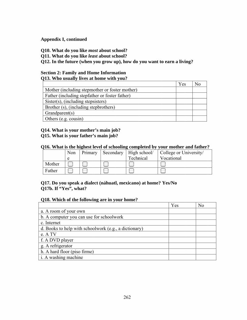
Ap Q1Q1Q1 SecQ1

MFSBGO

Q1Q1 Q1

MF

Q1Q1 Q1 a. Ab. Ac. Id. Be. Af. Ag. Ah. Ai. A

ppendix I, co

10. What do11. What do12. In the fu

ction 2: Fam13. Who usu

Mother (inclFather (incluSister(s), (incBrother (s), (GrandparentOthers (e.g. c

14. What is y15. What is y

16. What is tNe

Mother Father

17. Do you s17b. If “Yes

18. Which of

A room of yoA computer Internet Books to helA TV A DVD playA refrigeratoA hard floorA washing m

ontinued

o you like moo you like leauture (when

mily and Houally lives at

luding stepmuding stepfatcluding step(including st(s) cousin)

your motheyour father

the highest Non

Prima

speak a diale”, what?

f the followi

our own you can use

lp with scho

yer or r (piso firme)

machine

ost about scast about scyou grow u

ome Informt home with

mother or fosther or fostersisters) tepbrothers)

er’s main jor’s main job

level of schoary Second

ect (náhuat

ing are in y

e for schoolw

olwork (e.g.

)

262

chool? chool? up), how do

ation h you?

ter mother)r father)

b? ?

ooling compdary High

Techn

l, mexicano

our home?

work

., a dictionar

you want to

pleted by yoschool/

nical CV

o) at home?

ry)

o earn a livi

Yes

our mother College or UVocational

Yes/No

Yes

ing?

s No

and father?University/

No

?

263

Appendix J. Principal Surveys

Q1. As of May 1, 2012 what was the total school enrollment (number of students)? (Please write a number in each line. Write 0 (zero) if there are none.)

a) Number of boys: __________ b) Number of girls: _____________

Q2. How many of the following teachers are on the staff of your school? Include both full- and part-time teachers. A full-time teacher is employed at least 90% of the time as a teacher for the full school year. All other teachers should be considered part-time. (Please write a number in each space provided. Write 0 (zero) if there is none.) Full-time Part-time Total Teachers Teachers certified by the SEP (Maestros certificados por la Secretaría de Educación Pública)

Teachers with other qualifications (Maestros egresados de una licenciatura en educación normalista, licenciatura universitaria, licenciatura tecnológica, especialización o maestría)

Q3. Is your school’s capacity to provide instruction hindered by any of the following issues? (Please tick one box in each row)

Not at all

Very little

To some extent

A lot

a) A lack of qualified science teachers b) A lack of qualified mathematics teachers c) A lack of qualified English teachers d) A lack of qualified teachers of other subjects Which subjects?

e) A lack of library staff f) A lack of other support personnel g) Shortage or inadequacy of science lab equipment h) Shortage or inadequacy of instructional materials (e.g. textbooks) which materials?

i) Shortage or inadequacy of computers for instruction j) Lack or inadequacy of Internet connectivity k) Shortage or inadequacy of computer software for instruction

l) Shortage or inadequacy of library materials Which materials would be helpful?

m) Shortage or inadequacy of audio-visual resources Q3n. Additional details about what they are lacking:

264

Appendix J, continued Q3.o. What do you see as the top 3 challenges for educating students in your school? In general? (Are they the same?) Q4. Approximately how many computers are available in your school?

a) What are they primarily used for? b) Approximately how many of these computers are connected to the Internet? c) Where are they located in the school? d) How often do students have access to the computers?

Daily Weekly Once a month Q5. Does your school have a library? Sí / No

a) If yes, approximately how many books? _____________________________ b) How long can students keep books out for? c) Do you have any newspaper subscriptions? Sí / No C1. If no, would you want some? Which ones?

C2. If yes, which ones? d) Do you have any magazine subscriptions? Sí / No

D1. If no, would you want some? Which ones? D2. If yes, which ones?

Q6. Regarding your school, who has a considerable responsibility for the following tasks? (Please tick as many boxes as appropriate in each row)

Principals Teachers School Governing board

Regional or local education authority

National education authority

a) Selecting teachers for hire b) Firing teachers c) Establishing teachers’ starting salaries

d) Determining teachers’ salaries increases

e) Formulating the school budget

f) Deciding on budget allocations within the school

g) Establishing student disciplinary policies

h) Establishing student assessment policies

i) Approving students for admission to the school

j) Choosing which textbooks are used

Appendix J, continued

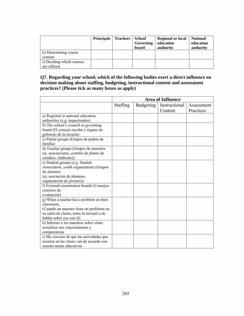
265

Principals Teachers School Governing board

Regional or local education authority

National education authority

k) Determining course content

l) Deciding which courses are offered

Q7. Regarding your school, which of the following bodies exert a direct influence on decision making about staffing, budgeting, instructional content and assessment practices? (Please tick as many boxes as apply)

Area of Influence Staffing Budgeting Instructional

Content Assessment Practices

a) Regional or national education authorities (e.g. inspectorates)

b) The school’s council or governing board (El consejo escolar y órgano de gobierno de la escuela)

c) Parent groups (Grupos de padres de familia)

d) Teacher groups (Grupos de maestros (ej. asociaciones, comités de planes de estudios, sindicato))

e) Student groups (e.g. Student Association, youth organisation) (Grupos de alumnos (ej. asociación de alumnos, organización de jóvenes))

f) External examination boards (Consejos externos de evaluación)

g) When a teacher has a problem en their classroom, (Cuando un maestro tiene un problema en su salón de clases, tomo la iniciativa de hablar sobre eso con él)

h) Informo a los maestros sobre cómo actualizar sus conocimientos y competencias

i) Me cercioro de que las actividades que ocurren en las clases van de acuerdo con nuestra metas educativas

266

Appendix J, continued Q8. About what percentage of students in your school repeated a grade last academic year? (Please write a number in each row. Write 0 (zero) if nobody repeated a grade.) The approximate

percentage of students repeating this grade

Grade not available in this school

a) First grade of middle school (Primer grado de Secundaria)/7th grade

b) Second grade of middle school (Segundo grado de Secundaria)/8th grade

c) Third grade of middle school (Tercer grado de Secundaria)/9th grade

d) First grade of high school (Primer grado de prepa)/10th grade

e) Second grade of high school (Segundo grado de prepa)/11th grade

f) Third grade of high school (Tercer grado de prepa)/12th grade

Q9. About what percentage of your total funding for a typical school year comes from the following sources? (Please write a number in each row. Write 0 (zero) if no funding comes from that source.) % a) Local Government (includes departments) b) Municipal Government c) Regional Government d) State Government e) National Government f) Student fees or school charges paid by parents g) Benefactors, donations, bequests, sponsorships, parent fund raising h) Other

TOTAL 100% Q10. About what percentage of your total funding for a typical school year goes to the following sources? (Please write a number in each row. Write 0 (zero) if no funding comes from that source.) % a) Teachers b) Non-Teacher Personnel (Administrative, teaching assistants, etc) c) Building maintenance/infrastructure d) Curriculum/teaching materials e) Financial aid (meals, fees, etc) f) other (describe) Total 100%

267

Appendix J, continued Q11. May I see a copy of your budget? Yes / No Q12. Approximately what percent of your student population receives Oportunidades monies?

a. Do you think Oportunidades has helped keep students in school? Q13. What percent of your graduating students do you think will go on to …

% High school Vocational school College/university

Q14. For those students that do not go to high school or vocational school, what types of jobs do you think they will have next year? In 5 year’s time?

Q15. How much of an impact do you think school has had on your students in terms of their future? A lot / a little / Not much / None

268

Appendix K. Occupation Rankings

Level Description/Criteria Occupations High School

student Preferences*

1 Manual labor intensive

Worker does not need to be literate

No formal education required

Day laborer Homemaker Launderer Shoe shiner Builder’s assistant

1 (1%)

2 Some manual labor required (though less than for level 1 jobs)

Some literacy and math skills needed

Primary education helpful if not required

Taxi driver Truck/delivery truck driver Painter Farmer Rancher Seamstress Stylist Cook Soldier Security guard Street or small shop vendor

1 (1%)

3 May require some manual labor

Worker needs to be literate

An elementary if not middle school education would be helpful if not required – no certification or degrees are necessary

Auto mechanic Plumber Carpenter Blacksmith Chef Secretary Miner Electrician Librarian Fireman Builder/basic construction

10 (10%)

4 Requires a low level university or vocational degree

Teacher Nurse Police Officer Accountant Administrator Network engineer/computer systems expert

60 (59%)

5 Requires a high level university degree

Lawyer Medical doctor University professor/researcher Architect Engineer

29 (29%)

*Of the 132 high school students who responded to survey questions, 101 (77%) answered this question (Q12). The middle school students who responded to survey questions varied considerably at the individual level. For example, one student wanted to either become a doctor or work in a rodeo. Due to the nature of student responses, only high school student responses could be coded with clarity and these are reported.