Embed Size (px)
Citation preview
Edinburgh Research Explorer
Energy Efficient Resource Allocation for Multiuser RelayNetworks
Citation for published version:Singh, K, Gupta, A & Ratnarajah, T 2016, 'Energy Efficient Resource Allocation for Multiuser RelayNetworks' IEEE Transactions on Wireless Communications. DOI: 10.1109/TWC.2016.2641961
Digital Object Identifier (DOI):10.1109/TWC.2016.2641961
Link:Link to publication record in Edinburgh Research Explorer
Document Version:Peer reviewed version
Published In:IEEE Transactions on Wireless Communications
General rightsCopyright for the publications made accessible via the Edinburgh Research Explorer is retained by the author(s)and / or other copyright owners and it is a condition of accessing these publications that users recognise andabide by the legal requirements associated with these rights.
Take down policyThe University of Edinburgh has made every reasonable effort to ensure that Edinburgh Research Explorercontent complies with UK legislation. If you believe that the public display of this file breaches copyright pleasecontact [email protected] providing details, and we will remove access to the work immediately andinvestigate your claim.
Download date: 29. Aug. 2018
1
Energy Efficient Resource Allocation
for Multiuser Relay NetworksKeshav Singh, Member, IEEE, Ankit Gupta, and Tharmalingam Ratnarajah, Senior Member, IEEE
Abstract—In this paper, a novel resource allocation algorithmis investigated to maximize the energy efficiency (EE) in multiuserdecode-and-forward (DF) relay interference networks. The EEoptimization problem is formulated as the ratio of the spectrumefficiency (SE) over the entire power consumption of the networksubject to total transmit power, subcarrier pairing and allocationconstraints. The formulated problem is a nonconvex fractionalmixed binary integer programming problem, i.e., NP-hard tosolve. Further, we resolve the convexity of the problem by aseries of convex transformations and propose an iterative EEmaximization (EEM) algorithm to jointly determine the optimalsubcarrier pairing at the relay, subcarrier allocation to each userpair and power allocation to all source and the relay nodes.Additionally, we derive an asymptotically optimal solution byusing the dual decomposition method. To gain more insights intothe obtained solutions, we further analyze the resource allocationalgorithm in a two-user case with interference-dominated andnoise-dominated regimes. In addition, a suboptimal algorithmis investigated with reduced complexity at the cost of acceptableperformance degradation. Simulation results are used to evaluatethe performance of the proposed algorithms and demonstrate theimpacts of various network parameters on the attainable EE andSE.
Index Terms—Energy efficiency, resource allocation, multiuser,decode-and-forward, relay networks.
I. INTRODUCTION
The cooperative communication and small cell have
emerged as promising future technologies for improving the
network throughput, enlarging the transmission range of wire-
less networks and enhancing the link reliability [1]. The relay
networks can swiftly increase the spectral efficiency (SE) of
the network. However, the power dissipation, which is not
only due to transceiver but also due to complete radio access
network, increases significantly and are predicted to surge
rapidly and reach to the current level of the total electricity
consumption in the next 20-25 years [2]. To enhance the
energy efficiency (EE) of wireless networks is of paramount
importance in realizing 5G radio access solutions. Conse-
quently, it is urgent to investigate energy-aware architecture
and resource allocation techniques that prolong the network
Manuscript received June 4, 2016; revised September 25, 2016; acceptedDecember 06, 2016. The associate editor coordinating the review of this paperand approving it for publication was Prof. Shi Jin.
This work was supported by the U.K. Engineering and Physical SciencesResearch Council (EPSRC) under Grant EP/L025299/1.
Keshav Singh and Tharmalingam Ratnarajah are with the Institute for Digi-tal Communications, the University of Edinburgh, Kings Building, Edinburgh,UK, EH9 3JL. E-mails: K.Singh; [email protected].
Ankit Gupta is with Aricent Technologies Limited (Holdings), Gurgaon,India. E-mail: [email protected].
The corresponding author of this paper is Keshav Singh.
lifespan or provide significant energy savings under the um-
brella of the green communications [3].
Various relaying protocols have been proposed for coop-
erative networks, among which amplify-and-forward (AF),
decode-and-forward (DF) [1] and compress-and-forward (CF)
[4] are three common ones. In AF protocol, the relay re-
transmits the amplified signal to the destination, whereas
in the DF protocol, the relay first attempts to decode the
received signal and then forwards the re-encoded information
bits to the destination. In CF protocol, the relay compresses
the received signal and sends the compressed signal to the
destination. The AF protocol has an advantage over others
in terms of low implementation complexity. However, the DF
protocol performs better than other two protocols when the
channel quality of forward links, i.e., source-to-relay (SR)
links is good enough. Another advantage of the DF protocol
is that it is possible to use different channel coding schemes
at the source and the relay nodes and the transmission can
be optimized for both links. i.e., SR and relay-to-destination
(RD), separately. Moreover, multiuser interference channel
in a relay-assisted network becomes a major bottleneck for
improving the networks performance due to the increase in
the number of interfering sources. Exploiting multicarrier,
resource management, and beamforming techniques, users
in the network can share the resources and alleviate severe
interference generated from other users. Thus, in this paper,
we investigate resource allocation in multiuser DF relay inter-
ference network for enhancing the energy utilization among
users, and illustrate the impact of various network parameters
on the performance tradeoff between the EE and SE.
In recent years, the energy dissipation at battery-powered
mobile devices has increased rapidly due to the diverse
and ubiquitous wireless services. Unfortunately, we cannot
increase the battery capacity of devices because of the slow
advance of battery technology and size limit. Thus, the opti-
mization of power usage in multiuser relay networks becomes
a critical issue. However, the interference, energy consumption
and throughput can be controlled through optimization of
resource usage. The power dissipation in wireless networks are
generally classified into two main categories: dynamic power
dissipation and static power dissipation. The dynamic power
dissipation denotes the transmit power which is allocated in
response to the instantaneous channel conditions, whereas the
static power dissipation covers site cooling, signal processing
at each node and battery backup [5]. The EE performance
of multiuser multicarrier DF relay networks highly depends
on these two sources [6]. In this paper, we will focus on
maximizing the EE of the DF relay interference network by
2
joint optimization of resource allocation with consideration of
the dynamic and the total static power consumption.
Recently, resource allocation schemes have been studied for
improving the performance of the DF relay networks [7]–[14].
In [7] and [8], the optimal power allocation policies were
investigated for rate maximization of the DF networks under
a sum power constraint, or individual power constraints at
the source and the relay nodes. However, the joint subcarrier
and power allocation was not addressed in [7] and [8]. To
further improve the network performance, the optimization
problem for joint subcarrier and power allocation with a total
network power constraint or with individual power constraints
for the source and the relay nodes were formulated in [9]–
[14]. The works in [9] studied the subcarrier pairing and power
allocation problem for AF and DF schemes under a total power
constraint and provided the optimality of ordered subcarrier
pairing (OSP) without diversity. To overcome the interference,
the authors in [10] jointly optimized power allocation, relay se-
lection and subcarrier assignment. The optimal subcarrier and
power allocation schemes were investigated in [11] for a two-
hop DF orthogonal frequency and code division multiplexing
(OFCDM) based relay network and analyzed the effects of
the channel state information (CSI) under the relay and
direct-link mode, whereas the subcarrier-pairing and power
allocation were optimized to maximize the weighted sum rate
for a point-to-point orthogonal frequency division multiplexing
(OFDM) with DF relay network in [12]. Under a perfect self-
interference cancellation, a joint resource allocation scheme
for orthogonal frequency division multiple access (OFDMA)
assisted multiuser two-way AF relay network was proposed
in [14] for maximizing the total sum rate. In [9]–[14], the
optimization of sum rate, power and subcarrier allocation in
high signal-to-noise ratio (SNR) region was the focal point
for achieving higher system throughput without concerning
the energy dissipation in the networks and balancing the sum
rate of different links. Many recent research works on energy
efficient resource allocation have been reported in [6], [15]–
[19]. The utility-based dynamic resource allocation algorithm
in relay-aided OFDMA system was investigated in [15] for
maximizing the average utility of all users with multiservice,
whereas the issue has not been studied from the viewpoint
of the EE. In [16], an energy efficient resource scheduling
solution for downlink transmission in multiuser OFDMA
networks was proposed under imperfect CSI, while the authors
in [17] extended the work of [16] for multicarrier under perfect
CSI knowledge and studied the joint subcarrier and power
allocation problem under a total power constraint for downlink
multiuser OFDMA system. The resource allocation problem
in [16] and [17] was optimized only in downlink scenario for
maximizing EE without considering the multiuser interference
in the network which could be a restraining factor in the
performance enhancement when the number of mobile users
increases. The only power allocation policies for enhancing
EE of AF networks were considered in [19]. However, the
optimal joint subcarrier and power allocation schemes for DF
relay networks will not be same when we consider the network
EE as objective function. Therefore, there is a need to revisit
the design of existing DF relay interference networks and
investigate the associated resource allocation policies in order
to improve the network EE. To the best of authors knowledge,
no work has been reported yet on EE maximization problem by
jointly considering subcarrier pairing permutation, subcarrier
allocation, and power optimization in multiuser DF relay
interference network, in which the multiuser interference could
be a restraining factor in the performance enhancement when
the number of users increases.
In this paper, we consider a joint resource allocation prob-
lem in multiuser multicarrier DF relay networks, where all
the nodes in the network are equipped with a single antenna
and users communicate with each other through a single half-
duplex DF relay node. The major contributions and ingenious
novelty of our work are summarized as follows. We formulate
EE maximization (EEM) problem in the context of a multiuser
DF relay interference network as a ratio of the total achievable
sum rate over the entire power consumption in the network
subject to a total transmit power constraint, which jointly
addresses both the subcarrier and power allocation. Unlike [9]–
[14], in this paper, the primary goal is to maximize EE. Since,
the original optimization problem is nonconvex fractional
mixed binary integer programming problem, i.e. NP-hard to
solve, we use successive convex approximation (SCA) [20]
and continuous convex relaxations to transform the problem
into tractable convex one. Next, the joint quasi-concavity of
EE problem on joint subcarrier and power allocation matrices
is derived and based on the optimization results, we obtain an
asymptotically optimal solution by using dual decomposition
method. Furthermore, to gain more insights into the optimal
solutions, we consider energy efficient joint resource alloca-
tion for two-user scenario and analyze the optimal resource
allocation algorithms in interference-dominated and noise-
dominated regimes. Besides, we also propose a suboptimal al-
gorithm with abridged complexity but acceptable performance
degradation. The complexity of the proposed algorithms is
further analyzed. The performance of the proposed algorithms
and the impact of various network parameters on the attainable
EE and SE are demonstrated through computer simulations.
The remainder of this paper is organized as follows. In
Section II, we describe the network model of multiuser re-
lay transmission, introduce the power dissipation model, and
formulate the joint resource allocation optimization problem.
Transformation of EE nonconvex optimization problem into
convex is illustrated in Section III. An energy efficient iterative
resource allocation algorithm for achieving the maximum EE
is presented in Section IV. We then analyze the resource
allocation policies for two-user cases under two different
operating regimes in Section V. The suboptimal resource allo-
cation algorithm is investigated in Section VI. The complexity
analysis of the proposed algorithms is presented in Section
VII, followed by the simulation results in Section VIII. Finally,
the conclusions are given in Section IX.
Notations: The following notation conventions are consid-
ered in this paper. Boldface lowercase and uppercase letters
(e.g., a and A) are used to represent a vector and a matrix,
respectively. The notations (·)† and E (·) denote the conjugate
transpose and expectation, respectively.

3
II. SYSTEM MODEL AND PROBLEM FORMULATION
A. System Model
We consider a multiuser DF relay network with Nsc sub-
carriers as illustrated in Fig.1, where N source nodes (Si,
for i = 1, ..., N ) concurrently transmit the signals to their
designated destination nodes (Di, for i = 1, ..., N ) by the
assistance of an intermediate relay node (R). It is assumed
that each node operates with only one antenna that does
not transmit and receive signals simultaneously. The SR and
RD channels on any subcarrier are assumed to be Rayleigh
frequency flat fading. Also assume that there is no direct
link between the source and the destination nodes due to the
path loss and large-scale fading. For simplicity, we assume
that the relay node has a perfect knowledge of CSI of each
link. Further, the relay node operates in a half-duplex mode
using DF scheme with two transmission phases. In the mul-
tiple access (MA) phase, all the source nodes(transmit users)
transmit their signals simultaneously to the relay node, while
the relay retransmits the re-encoded signals to the destination
nodes(receive users) in the broadcast (BC) phase; meanwhile
the source nodes remain inactive.
15
1311
S1
S2
S3
SN
Relay
(R)
D1
D2
D3
DN
145
12
82
6 9 4 10
151
13
106 314
72
BC Phase
MA Phase
N User Pairth
1 User Pairst
1
3
7 8
12
11
4
9
5
1 ... ...... scN 1 ... ...... scN
1 ... ...... scN
Available Subcarriers
Allocated Subcarriers
Fig. 1. A dual-hop mulituser DF relay network.
In the MA phase, the received signal at the relay node on
the m-th subcarrier is given by
y(m)R =
N∑
i=1
√
P(m)S,i h
(m)SiR
x(m)i + n
(m)R , (1)
where h(m)SiR
is the channel coefficient from the i-th source
node to the relay node on the m-th subcarrier, x(m)i denotes
the transmitted signal from the i-th source node on the m-th
subcarrier with unit power, i.e., E
[∣∣∣x
(m)i
∣∣∣
2]
= 1, P(m)S,i repre-
sents the transmit power of the i-th source node on the m-th
subcarrier, and n(m)R denotes the zero-mean complex additive
white Gaussian noise (AWGN) with variance(
σ(m)R
)2
. From
(1), the signal-to-interference plus noise ratio (SINR) at the
relay node for the i-th source node on the m-th subcarrier can
be given as
γ(m)SiR
=P
(m)S,i
∣∣∣h
(m)SiR
∣∣∣
2
N∑
j=1,j 6=i
P(m)S,j
∣∣∣h
(m)SjR
∣∣∣
2
+(
σ(m)R
)2, (2)
By assuming that the SR links are sufficiently good enough
to allow the sophisticated DF relay node for successfully
decoding the received signal, i.e., x(n)i = x
(n)i . Thus, in the
BC phase, the received signal at the i-th destination node on
the n-th subcarrier can be represented as
y(n)D,i = h
(n)RDi
N∑
i=1
√
P(n)R,i x
(n)i + n
(n)Di
;
= h(n)RDi
√
P(n)R,i x
(n)i
︸ ︷︷ ︸
Desired signal
+ h(n)RDi
N∑
j=1,j 6=i
√
P(n)R,j x
(n)j
︸ ︷︷ ︸
Interference
+n(n)Di︸︷︷︸
Noise
, (3)
where x(n)i is the decoded signal, h
(n)RDi
can be defined similar
to h(m)SiR
for RD links, P(n)R,i indicates the transmit power of
the relay node for the i-th source node on the n-th subcarrier,
and n(n)Di
can be describe similar to n(m)R but with variance
(
σ(n)Di
)2
. Using (3), the SINR at the i-th destination node on
the n-th subcarrier can be written as
γ(n)RDi
=P
(n)R,i
∣∣∣h
(n)RDi
∣∣∣
2
N∑
j=1,j 6=i
P(n)R,j
∣∣∣h
(n)RDi
∣∣∣
2
+(
σ(n)Di
)2, (4)
Define ρm,n ∈ 0, 1, ∀m,n, as the subcarrier pairing
indicator variable, where ρm,n = 1 if the m-th subcarrier in the
MA phase is paired with the n-th subcarrier in the BC phase,
and ρm,n = 0 otherwise. Further, Φi,(m,n) ∈ 0, 1, ∀i,m, n,
denotes the subcarrier allocation variable, where Φi,(m,n) = 1if the (m,n)-th subcarrier pair is assigned to the the i-th user
pair while Φi,(m,n) = 0 for the rest of the user pairs.
From (2) and (4), the achievable sum rate for the i-th user
pair can be evaluated as
Ri =
Nsc∑
m=1
Nsc∑
n=1
1
2ρm,nΦi,(m,n) log2
(
1 + min
γ(m)SiR
, γ(n)RDi
)
,
[bits/s/Hz] , (5)
where1
2comes from the fact that transmission consists of two
phases. Furthermore, the total sum rate of the network can be
given as
RTotal =N∑
i=1
Ri
=
N∑
i=1
Nsc∑
m=1
Nsc∑
n=1
1
2ρm,nΦi,(m,n) log2
(
1 + min
γ(m)SiR
, γ(n)RDi
)
,
[bits/s/Hz] , (6)
4
B. Power dissipation model
The power dissipation plays a paramount role in design-
ing of an energy efficient devices. In general, the required
quality-of-service (QoS) can even be obtained by utilizing
significantly less amount of power. In the network, the power
is dissipated in two ways namely: 1) transmit power; and 2)static power. The transmit power depends on the instantaneous
channel gains, whereas the static power includes the circuit and
processing powers utilized for signal detection and processing
performed by various circuitry components presented at the
relay and the destination nodes, and thus it directly depends on
the number of antennas [21] and remains constant for a node,
irrespective of its channel conditions. Therefore, the actual
power dissipation in the network after subcarrier pairing and
allocation can be written as
PTotal =N∑
i=1
Nsc∑
m=1
Nsc∑
n=1
ρm,nΦi,(m,n)
(
P(m)S,i + P
(n)R,i
)
︸ ︷︷ ︸
Dynamic Power
+ PSc + PRc︸ ︷︷ ︸
Static Power,Pc>0
[Watts] , (7)
where(
P(m)S,i + P
(n)R,i
)
denotes the total dynamic power con-
sumed by the source and relay nodes for transmission between
i-th user pair on the m-th and n-th subcarriers, respectively,
whereas PSc and PRc are the circuit and processing powers
together denoting the static power (Pc > 0) of the network. It
is observed that static power in (7) remains constant, whereas
the transmit power differs.
C. Primal Problem Formulation
The main objective of this work is to maximize the EE
of the relay network by jointly optimizing the subcarrier and
power allocation. Using (6) and (7), the EE of the network is
stated as follows.
Definition 1: The EE of the network can be defined as a
ratio of the minimum achievable sum rate to the total power
consumption1:
ηEE
(
P(m)S ,P
(n)R ,ρ,Φ
)
=RTotal
(
P(m)S ,P
(n)R ,ρ,Φ
)
PTotal
(
P(m)S ,P
(n)R ,ρ,Φ
) , (8)
where P(m)S =
[
P(m)S,1 , P
(m)S,2 , ..., P
(m)S,N
]T
and P(n)R =
[
P(n)R,1, P
(n)R,2, ..., P
(n)R,N
]T
denote the source and relay power
vectors for the m-th and n-th subcarriers, respectively, whereas
ρ = ρm,n and Φ = Φi,(m,n) express matrices for the
subcarrier pairing and allocation, respectively. Thus, the primal
1Since the function ηEE
(
P(m)S
, P(n)R
,ρ,Φ)
is nonconcave, the optimalityhere is defined in a locally optimal sense.
optimization problem can be formulated as follows:
(P1) maxP(m)S
,P(n)R
,ρ,Φ
ηEE
(
P(m)S ,P
(n)R ,ρ,Φ
)
s.t. (C.1)
N∑
i=1
Nsc∑
m=1
Nsc∑
n=1
ρm,nΦi,(m,n)
(
P(m)S,i + P
(n)R,i
)
≤Pmax;
(C.2)
Nsc∑
m=1
ρm,n = 1 , ∀ n ;
(C.3)
Nsc∑
n=1
ρm,n = 1 , ∀ m ; (9)
(C.4)
N∑
i=1
Φi,(m,n) = 1 , ∀ (m,n) ;
(C.5) ρm,n ∈ 0, 1, Φi,(m,n) ∈ 0, 1 , ∀ i,m, n ;
(C.6) P(m)S,i ≥ 0, P
(n)R,i ≥ 0 , ∀ i,m, n ,
where Pmax is the total transmit power budget of the network.
The constraint (C.1) limits the total transmit power utilized by
the source and the relay nodes and the constraints (C.2) and
(C.3) ensure that each subcarrier in the MA phase is paired
with one and only one subcarrier in the BC phase; and the
last constraint (C.4) guarantees that (m,n)-th subcarrier pair
is allocated to at least one user pair. According to [22], the
maximum sum rate in multiuser scenario can be achieved for
the case when each subcarrier is occupied by only one user
in each transmission. Therefore, each subcarrier is assigned
to only one user in the designed framework. The proposed
design framework can be easily extended to accommodate the
scenario where each subcarrier in the first hop can be paired
with one or more subcarriers in second hop and vice versa by
modifying the constraints (C.2) and (C.3) in (9) as follows:
(C.2) 1 ≤Nsc∑
m=1
ρm,n ≤ Nsc , ∀ n ;
(C.3) 1 ≤Nsc∑
n=1
ρm,n ≤ Nsc , ∀ m,
The new optimization problem can be solved in a similar way
as the problem (P1). However, the new optimization problem
requires the update of 2Nsc Lagrangian multipliers in the the
master problem, and thus exhibits high computational com-
plexity. Additionally, the Hungarian method cannot be directly
applied for solving the subcarrier pairing matrix ρ. Notice that
there is a tradeoff between performance and computational
complexity. Therefore, we consider the problem (P1) instead
of new optimization problem and investigate the EEM algo-
rithm to find the optimal resource allocation policy. In this
work, the relay node is equipped with only a single antenna,
however, the design framework can also be easily generalized
to the scenario with multiple antennas. In this case, the SR
and RD links become single input multiple output (SIMO) and
multiple input single output (MISO) channels, respectively. By
expertly designing receive and transmit beamforming weights
for the relay node, we can derive the SINR similar to (2) and
(4). In general, an increased number of antennas can offer

5
better interference suppression capability, but it also requires
more static power consumption and skillful subcarrier pairing
and allocation, thus leading to EE performance tradeoff.
III. TRANSFORMATION OF NONCONVEX OPTIMIZATION
PROBLEM
The optimization problem (P1) is nonconvex in nature due
to the fractional form of the objective function in (9) and a
mixed binary integer nonlinear programming problem [23].
There is no standard technique to solve such optimization
problem. Therefore, in order to determine the optimal re-
source allocation policies we need to transform the original
optimization problem (9) into an analytically tractable form
which will be convex in nature. By introducing the parameter
Γ(k)i ≥ 0, k = 1, . . . , Nsc, the optimization problem (P1) can
be rewritten as
(P2)
maxP(m)S
,P(n)R
ρ,Φ,Γ(k)
N∑
i=1
Nsc∑
m=1k=m
Nsc∑
n=1
1
2ρm,nΦi,(m,n) log2
(
1 + Γ(k)i
)
N∑
i=1
Nsc∑
m=1
Nsc∑
n=1ρm,nΦi,(m,n)
(
P(m)S,i + P
(n)R,i
)
+ Pc
s.t. (C.1)− (C.6) ;
(C.7) γ(k)SiR≥ Γ
(k)i , ∀ k ; (10)
(C.8) γ(k)RDi≥ Γ
(k)i , ∀ k ,
where Γ(k) = Γ
(k)i is a auxiliary variable vector. The SINR
in MA and BC phases must be greater than or equal to this
auxiliary variable. Furthermore, by applying the change of
variables P(m)S,i = lnP
(m)S,i , P
(n)R,i = lnP
(n)R,i and Γ
(k)i = lnΓ
(k)i ,
the problem (P2) can be equivalently written as
(P3)
maxP(m)S ,P
(n)R
ρ,Φ,Γ(k)
F(
ρ,Φ,Γ(m)
)
︷ ︸︸ ︷
N∑
i=1
Nsc∑
m=1
Nsc∑
n=1
1
2ρm,nΦi,(m,n) log2
(
1 + eΓ(m)i
)
N∑
i=1
Nsc∑
m=1
Nsc∑
n=1ρm,nΦi,(m,n)
(
eP(m)S,i + eP
(n)R,i
)
+ Pc
s.t. (C.1)
N∑
i=1
Nsc∑
m=1
Nsc∑
n=1
ρm,nΦi,(m,n)
(
eP(m)S,i + eP
(n)R,i
)
≤Pmax;
(C.2)− (C.5) ; (11)
(C.7)
N∑
j=1,j 6=i
eΓ(k)i
−P(k)S,i
+P(k)S,j
∣∣∣h
(k)SjR
∣∣∣
2
∣∣∣h
(k)SiR
∣∣∣
2
+ eΓ(k)i
−P(k)S,i
(
σ(k)R
)2
∣∣∣h
(k)SiR
∣∣∣
2 ≤ 1 , ∀ i, k ;
(C.8)
N∑
j=1,j 6=i
eΓ(k)i
−P(k)R,i
+P(k)R,j
∣∣∣h
(k)RDj
∣∣∣
2
∣∣∣h
(k)RDi
∣∣∣
2
+ eΓ(k)i
−P(k)R,i
(
σ(k)Di
)2
∣∣∣h
(k)RDi
∣∣∣
2 ≤ 1, ∀ i, k ,
Because of the fractional form, the objective function in (11) is
nonconvex. By utilizing the properties of nonlinear fractional
programming [24] which is useful to deal with concave-over-
convex fractional function in an iterative manner, we can
transform the objective function in a subtractive form. To
make the objective function concave-over-convex, we use SCA
method to impose a lower bound on F (ρ,Φ, Γ(m)
) [6], [20];
it yields
F (ρ,Φ, Γ(m)
)
≥N∑
i=1
Nsc∑
m=1
Nsc∑
n=1
1
2ρm,nΦi,(m,n)
(
α(m)i
ln(2)Γ(m)i + β
(m)i
)
;
, FLB
(
ρ,Φ, Γ(m)
,α(m),β(m))
, (12)
where α(m) =[
α(m)1 , α
(m)2 , ..., α
(m)N
]
and β(m) =[
β(m)1 , β
(m)2 , ..., β
(m)N
]
are the coefficients determined in the
following manner [6]
α(m)i =
ς(m)i
1 + ς(m)i
; (13)
β(m)i = log2
(
1 + ς(m)i
)
− α(m)i log2
(
ς(m)i
)
, (14)
for any ς(m)i > 0. Note that the equality in (12)
satisfied when α(m)i = Γ
(m)i
/1 + Γ
(m)i and β
(m)i =
log2
(
1 + Γ(m)i
)
− α(m)i log2
(
Γ(m)i
)
, and the equality holds
only if(
α(m)i , β
(m)i
)
= (1, 0) and Γ(m)i → ∞. After substi-
tuting (12) in (P3), the problem in (11) can be reformulated
as
(P4)
maxP(m)S ,P
(n)R
ρ,Φ,Γ(m)
FLB
(
ρ,Φ, Γ(m)
,α(m),β(m))
N∑
i=1
Nsc∑
m=1
Nsc∑
n=1ρm,nΦi,(m,n)
(
eP(m)S,i + eP
(n)R,i
)
+ Pc
s.t. (C.1)− (C.5) , (C.7)& (C.8) , (15)
Since the objective function in (15) is in a form of concave-
over-convex for fixed subcarrier pairing and allocation, we can
apply nonlinear programming method [24] to transform the
problem into a convex optimization problem as
(P5)max
P(m)S ,P
(n)R ,ρ,Φ,Γ
(m)FLB
(
P(m)
S , P(n)
R ,ρ,Φ, Γ(m)
,α(m),β(m))
s.t. (C.1)− (C.5) , (C.7)& (C.8) , (16)
where FLB
(
P(m)
S , P(n)
R ,ρ,Φ, Γ(m)
,α(m),β(m))
= FLB −
Ψ
(N∑
i=1
Nsc∑
m=1
Nsc∑
n=1ρm,nΦi,(m,n)
(
eP(m)S,i + eP
(n)R,i
)
+ Pc
)
and Ψ
is a non-negative parameter and works as a penalty factor for
the resource utilization. Note that when Ψ → 0, it implies
that the penalty to use the resources is almost zero, and the
resource allocation problem (16) is degenerated to a sum-
rate maximization problem. However, for another extreme case
where Ψ→∞, no resource allocation policy is good enough
to maximize the objective function in (16).
Lemma 1: For fixed subcarrier pairing and allocation
(ρ,Φ), the lower bound in the problem (P5)
6
FLB
(
P(m)
S , P(n)
R ,ρ,Φ, Γ(m)
,α(m),β(m))
is concavified
by the change of variables P(m)S,i = lnP
(m)S,i , P
(n)R,i = lnP
(n)R,i
and Γ(m)i = lnΓ
(m)i , for any given α
(m)i , β
(m)i and Ψ.
Proof: After substituting P(m)S,i = eP
(m)S,i , P
(n)R,i =
eP(n)R,i and Γ(m) = eΓ
(m)
in (P2), the objective function
FLB
(
P(m)
S , P(n)
R ,ρ,Φ, Γ(m)
,α(m),β(m))
in (P5) can be
written as
FLB
(
P(m)
S , P(n)
R ,ρ,Φ, Γ(m)
,α(m),β(m))
=
N∑
i=1
Nsc∑
m=1
Nsc∑
n=1
1
2ρm,nΦi,(m,n)
(
α(m)i
2Γ(m)i + β
(m)i
)
(17)
−Ψ
(N∑
i=1
Nsc∑
m=1
Nsc∑
n=1
ρm,nΦi,(m,n)
(
eP(m)S,i + eP
(n)R,i
)
+ Pc
)
,
Since, α(m)i ≥ 0, β
(m)i ≥ 0 and Ψ ≥ 0, the objective function
(17) forms the summation of the concave terms and linear
terms (i.e. minus-exp functions) for given subcarrier pairing
and allocation (ρ,Φ), hence the objective function FLB is
concavified by nature.
We can solve the problem (P5) in two steps, firstly the
power allocation to each source and relay nodes is decoupled
with the problem of subcarrier pairing and allocation. Next,
the subcarrier allocation to each user pair is decoupled with
the problem of subcarrier pairing. In case of equal subcarrier
allocation and direct pairing, the total number of subcarriers
are equally divided between users and first subcarrier in SRphase is paired to first one in RD phase, respectively. Further,
the subcarrier pairing and allocation matrices are defined as
ρ = INsc and Φ = blkdiag (σ1, ...,σN ), respectively, where
σi = I⌊Nsc/N⌋, ∀ i = 1, ..., N . For the case of N = 2 and
Nsc = 2, we can find γ(m)SiR
, and γ(n)RDi
, m,n = 1, 2, using
(2) and (4), and the maximum achievable sum rate RA can
be computed using (6) for one-to-one mapping and user wise
allocation. While in case of the optimal subcarrier pairing and
allocation, the subcarriers are optimally allocated and paired
using (29) − (31), respectively, and the achievable sum rate
RB is computed.
Now, we have two cases for optimally allocated powers
limited by Pmax, the sum rate RA is calculated for fixed type
of subcarrier pairing, this leads to undesired interference and
noise, thereby leading to degradation of the sum rate RA, while
with the optimal power allocation, the subcarrier allocation
and pairing is also done optimally and thus we can notice that
RB > RA. According to [25], if RB exceeds RA, it is proven
that we can easily treat power allocation, and subcarrier pairing
and allocation as two separate problems, even for large number
of subcarriers. In a similar manner, we can also prove the
decoupling of subcarrier allocation and pairing for optimally
calculated power, wherein the sum rate with improper mapping
of subcarriers in two-hops significantly degrades as compare
to that of the sum rate with optimally allocated subcarrier
pairing and allocation, thereby, using [25], we can prove the
decoupling of subcarrier pairing and allocation.
IV. EE RESOURCE ALLOCATION ALGORITHM
The maximization problem (P1) is transformed into a mixed
binary integer nonlinear programming problem (P5), and thus
an exhaustive search over all variables is required to find the
global optimal solution. Consequently, the computational com-
plexity becomes very high. However, the duality gaps between
the primal problem and the dual problem in a multicarrier
system approaches to zero when the number of subcarriers
goes to infinity [26], [27]. The definition of duality gap and
related theorem are given as follows:
Definition 2 (Duality Gap): The difference in the optimal
solution of the optimization problem (P5), given by OP ⋆,
and its dual optimization problem in (20), given by DP ⋆,
is defined as duality gap, expressed as DG = OP ⋆ −DP ⋆.
Theorem 1: For sufficiently large number of subcarriers
Nsc, the duality gap DG tends to zero, i.e., DG = OP ⋆ −DP ⋆ ≈ 0.
Proof: Please see Appendix A.
Thus, we focus on solving the dual problem [23] instead of
the original problem and propose an iterative EEM algorithm
to find the optimal resource allocation policies that can maxi-
mize its lower bound under fixed coefficients α(m)i and β
(m)i ,
followed by an update of these two coefficients that guarantees
a monotonic increase in the lower bound performance.
A. Dual Problem Formulation
For fixed subcarrier pairing and allocation variables ρm,nand Φi,(m,n), the optimization problem (P5) is a convex
problem with given lower bound coefficients α(m)i and
β(m)i . Thus the Lagrangian function for the relaxed opti-
mization problem (P5) is expressed in (18), as shown on the
top of the next page, where λ, µ(k) =[
µ(k)1 , µ
(k)2 , ..., µ
(k)N
]T
and ν(k) =[
ν(k)1 , ν
(k)2 , ..., ν
(k)N
]T
are Lagrangian multipli-
ers associated with the constraints (C.1), (C.7) and (C.8),respectively. The Lagrangian dual function can therefore be
expressed as
g(
λ,µ(k),ν(k))
, maxP(m)S ,P
(n)R
ρ,Φ,Γ(m)
L(
P(m)
S , P(n)
R ,ρ,Φ, Γ(m)
, λ,µ(k),ν(k))
s.t. (C.2)− (C.5) , (19)
Then the dual optimization problem can be written as
minλ,µ(k),ν(k)≥0
g(
λ,µ(k),ν(k))
=
minλ,µ(k)≥0
ν(k)≥0
maxP(m)S ,P
(n)R
ρ,Φ,Γ(m)
L(
P(m)
S , P(n)
R ,ρ,Φ, Γ(m)
, λ,µ(k),ν(k))
,
s.t. (C.2)− (C.5) , (20)
The dual problem in (20) can be decomposed into a master
problem and a subproblem, and it can be solved in an iterative
manner until the convergence is reached.

7
L(
P(m)
S , P(n)
R ,ρ,Φ, Γ(m)
, λ,µ(k),ν(k))
= FLB
(
P(m)
S , P(n)
R ,ρ,Φ, Γ(m)
,α(m),β(m))
− λ
(N∑
i=1
Nsc∑
m=1
Nsc∑
n=1
ρm,nΦi,(m,n)
(
eP(m)S,i + eP
(n)R,i
)
− Pmax
)
−N∑
i=1
Nsc∑
k=1
µ(k)i
N∑
j=1,j 6=i
eΓ(k)i
−P(k)S,i
+P(k)S,j
∣∣∣h
(k)SjR
∣∣∣
2
∣∣∣h
(k)SiR
∣∣∣
2 + eΓ(k)i
−P(k)S,i
(
σ(k)R
)2
∣∣∣h
(k)SiR
∣∣∣
2 − 1
(18)
−N∑
i=1
Nsc∑
k=1
ν(k)i
N∑
j=1,j 6=i
eΓ(k)i
−P(k)R,i
+P(k)R,j
∣∣∣h
(k)RDj
∣∣∣
2
∣∣∣h
(k)RDi
∣∣∣
2 + eΓ(k)i
−P(k)R,i
(
σ(k)Di
)2
∣∣∣h
(k)RDi
∣∣∣
2 − 1
∣∣∣∣∣∣∣∣∣∣∣∣
Nsc∑
m=1ρm,n = 1 , ∀n;
Nsc∑
n=1ρm,n = 1 , ∀m;
N∑
i=1
Φi,(m,n) = 1 , ∀(m,n),
B. Solution of the Subproblem
From Lemma 1, the objective function in (9) is concave in(
P(m)
S , P(n)
R ,ρ,Φ, Γ(m))
, and thus the optimal solution can
be found by solving the Lagrange dual domain because the
duality gap between (16) and the dual problem is nearly zero
for large number of Nsc, in two steps for fixed Lagrangian
multipliers: 1) by using KKT [23] conditions which are first-
order imperative and sufficient conditions for optimality for
convex optimization problem, we can find the optimal power
allocation for each source and the relay nodes for given
subcarrier pairing ρ and subcarrier allocation Φ; and 2) find
the optimal ρ and Φ for the obtained power allocation in the
first step.
By taking the partial derivative of (18) with respect to
P(m)S,i , P
(n)R,i , Γ
(m)i and equating the results to zero, we get
the update equation for the power allocation and Γ(m)i at
the (t + 1)-th iteration as in (21)-(23), where ϕ =1
2,
=1
2 ln 2and [·]+ = max 0, ·. Since the m-th sub-
carrier is allocated to the i-th source node, the transmit
power allocated on the m-th subcarrier by other transmit
nodes is almost close to zero, and thus under assumption
of eΓ(m)i
(∑N
j=1,j 6=i eP
(m)S,j
∣∣∣h
(m)SjR
∣∣∣
2
+(
σ(m)R
)2)
≈ ∆S and
eΓ(n)i
(∑N
j=1,j 6=i eP
(n)R,j
∣∣∣h
(n)RDj
∣∣∣
2
+(
σ(n)Di
)2)
≈∆R, the opti-
mal power of the i−th source and the relay nodes at the
(t+1)-th iteration can be updated for given subcarrier paring
ρm,n = 1 and allocation Φi,(m,n) = 1 as follows:
P(m)S,i (t+ 1) =
ϕ
ln
µ(m)i ∆S
(Ψ + λ)∣∣∣h
(m)SiR
∣∣∣
2
+
; (24)
P(n)R,i (t+ 1) =
ϕ
ln
ν(n)i ∆R
(Ψ + λ)∣∣∣h
(n)RDi
∣∣∣
2
+
, (25)
The optimal power allocations in (24) and (25) are indeed
customized water-filling solutions and it can be observed that
the water levels are not only determined by the penalty of
allocating power λ, but also on the current penalty of the
power utilization to the EE given by Ψ. As can be seen from
(25), the relay node also follows similar power allocation
policy for the i-th source node’s signal in the second hop.
However, for without subcarrier pairing and allocation, the
power allocation policy needs to consider the interference
channel power generated from other source nodes towards the
i-th source node.
To derive the optimal subcarrier pairing and allocation, we
substitute P(m)⋆
S,i , P(n)⋆
R,i , and Γ(m)⋆
i into the (18), the dual
problem g(λ,µ(k),ν(k)
)becomes
g(
λ,µ(k),ν(k))
= maxρ,Φ
N∑
i=1
Nsc∑
m=1
Nsc∑
n=1
ρm,nΦi,(m,n)Bi,(m,n)
+ C(
P(m)⋆
S , P(n)⋆
R , Γ(m)⋆
, λ,µ(k),ν(k))
s.t. (C.1)− (C.5) , (26)
where Bi,(m,n) and C are defined as
Bi,(m,n) =(
α(m)i Γ
(m)⋆
i + ϕβ(m)i
)
−(Ψ + λ)(
eP(m)⋆
S,i + eP(n)⋆
R,i
)
; (27)
C(
P(m)⋆
S , P(n)⋆
R , Γ(m)⋆
, λ,µ(k),ν(k))
= −ΨPc + λPmax
−N∑
i=1
Nsc∑
k=1
µ(k)i
N∑
j=1,j 6=i
eΓ(k)⋆
i−P
(k)⋆
S,i+P
(k)⋆
S,j
∣∣∣h
(k)SjR
∣∣∣
2
∣∣∣h
(k)SiR
∣∣∣
2
+eΓ(k)⋆
i−P
(k)⋆
S,i
(
σ(k)R
)2
∣∣∣h
(k)SiR
∣∣∣
2 − 1
−N∑
i=1
Nsc∑
k=1
ν(k)i
N∑
j=1,j 6=i
eΓ(k)⋆
i−P
(k)⋆
R,i+P
(k)⋆
R,j
∣∣∣h
(k)RDj
∣∣∣
2
∣∣∣h
(k)RDi
∣∣∣
2
+eΓ(k)⋆
i−P
(k)⋆
R,i
(
σ(k)Di
)2
∣∣∣h
(k)RDi
∣∣∣
2 − 1
, (28)

8
P(m)S,i (t+ 1) =
ϕ
ln
µ(m)i eΓ
(m)i
N∑
j=1,j 6=i
eP(m)S,j
∣∣∣h
(m)SjR
∣∣∣
2
+(
σ(m)R
)2
− ln
(Nsc∑
n=1
ρm,nΦi,(m,n) (Ψ + λ)∣∣∣h
(m)SiR
∣∣∣
2)
+
;
(21)
P(n)R,i (t+ 1) =
ϕ
ln
ν(n)i eΓ
(n)i
N∑
j=1,j 6=i
eP(n)R,j
∣∣∣h
(n)RDj
∣∣∣
2
+(
σ(n)Di
)2
− ln
(Nsc∑
m=1
ρm,nΦi,(m,n) (Ψ + λ)∣∣∣h
(n)RDi
∣∣∣
2)
+
;
(22)
Γ(m)i (t+ 1) =
[
ln
(Nsc∑
n=1
ρm,nΦi,(m,n)α(m)i
)
− ln
(
µ(m)i e−P
(m)S,i
∣∣∣h
(m)SiR
∣∣∣
2
N∑
j 6=i
eP(m)S,j
∣∣∣h
(m)SjR
∣∣∣
2
+ σ(m)R
2
+ν(m)i e−P
(m)R,i
∣∣∣h
(m)RDi
∣∣∣
2
N∑
j 6=i
eP(m)R,j
∣∣∣h
(m)RDj
∣∣∣
2
+ σ(m)Di
2
)]+
, (23)
It can be observed that only Bi,(m,n) depends
on the subcarrier pairing and allocation, whereas
C(
P(m)⋆
S , P(n)⋆
R , Γ(m)⋆
, λ,µ(k),ν(k))
does not depend
on any subcarrier pairing and allocation. Furthermore, the
first term of Bi,(m,n) indicates the sum rate achieved by the
i-th user pair on the (m,n)-th subcarrier pairing, while the
second term works as penalty for power utilization.
For given subcarrier pairing matrix ρ and the optimal power
allocation(
P(m)⋆
S , P(n)⋆
R , Γ(m)⋆
)
for fixed coefficients α(m)i
and β(m)i , the optimal subcarrier allocation can be obtained
by solving the following problem:
g(
λ,µ(k),ν(k))
= maxΦ
N∑
i=1
Nsc∑
m=1
Nsc∑
n=1
ρ⋆m,nΦi,(m,n)Bi,(m,n)
+ C(
P(m)⋆
S , P(n)⋆
R , Γ(m)⋆
, λ,µ(k),ν(k))
s.t. (C.1) & (C.4) , (29)
In order to determine the optimal solution of (29), the i-thuser pair can be selected that maximizes Bi,(m,n) for a given
subcarrier pairing (m,n), i.e.,
Φ⋆i,(m,n) =
1, for i = argmaxi Bi,(m,n) ,
0, otherwise(30)
Lastly, to find the optimal subcarrier pairing ρ⋆, we substi-
tute (30) into (26), which yields
g(
λ,µ(k),ν(k))
= maxρ
N∑
i=1
Nsc∑
m=1
Nsc∑
n=1
ρm,nΦ⋆i,(m,n)Bi⋆,(m,n)
+ C(
P(m)⋆
S , P(n)⋆
R , Γ(m)⋆
, λ,µ(k),ν(k))
s.t. (C.1)− (C.3) , (31)
where Bi⋆,(m,n) = maxi Bi,(m,n) ∀ (m,n). The optimization
problem (31) can be efficiently solved by using the standard
Hungarian method [28] to find the optimal ρ⋆.
C. Master problem Solution: Update of Lagrangian Multipli-
ers
By utilizing the subgradient method, the dual variables λ,
µ(k) and ν(k) can be iteratively updated as in (32)-(34),
where ε1, ε2 and ε3 are positive step sizes. The optimal
resource allocation(
P(m)⋆
S , P(n)⋆
R ,ρ⋆,Φ⋆)
of the problem
(P5) can be found through the iterative procedure of (21)-
(23), (30), (31), and (32)-(34) for given coefficients α(m)i and
β(m)i and the penalty factor Ψ. The lower bound performance
FLB
(
P(m)
S , P(n)
R ,ρ,Φ,α(m),β(m))
depends on the two co-
efficients α(m) and β(m), and thus by carefully choosing the
values of these two coefficients, the lower bound performance
of FLB
(
P(m)
S , P(n)
R ,ρ,Φ,α(m),β(m))
depends on the two
coefficients α(m) and β(m) can be enhanced. Next, we will
provide the theorem regarding the update of α(m) and β(m).
Theorem 2: If the coefficients α(m)i (t) and β
(m)i (t) are
updated as
α(m)i (t+ 1) =
Γ(m)i (t)
1 + Γ(m)i (t)
; (35)
β(m)i (t+ 1) = log2
(
1 + Γ(m)i (t)
)
− α(m)i (t+ 1) log2
(
Γ(m)i (t+ 1)
)
, (36)
for the optimal solution(
P(m)⋆
S (t), P(n)⋆
R (t),ρ⋆(t),Φ⋆(t),
Γ(m)⋆
(t))
of the problem (P5) at the t-th inner iteration, then
the optimal value of FLB
(
P(m)
S , P(n)
R ,ρ,Φ,α(m),β(m))
in
(16) is monotonically increased. Also, after the convergence
of the coefficients α(m)i (t) and β
(m)i (t), the optimal solution
for (P5) behaves as the local maximizer for the problem (P1).
Proof: The proof is relegated in Appendix B.
The penalty factor Ψ which is defined as the ratio of
the achievable sum rate to the total power consumption in
the network works as network EE. For a given Ψ, we first
introduce an iterative EEM algorithm which is summarized
9
λ(t+ 1)=
[
λ(t) + ε1(t)
(N∑
i=1
Nsc∑
m=1
Nsc∑
n=1
ρ⋆m,nΦ⋆i,(m,n)
(
eP(m)⋆
S,i + eP(n)⋆
R,i
)
− Pmax
)]+
; (32)
µ(m)i (t+ 1)=
µ
(m)i (t) + ε2(t)
N∑
j=1,j 6=i
eΓ(m)⋆
i−P
(m)⋆
S,i+P
(m)⋆
S,j
∣∣∣h
(m)SjR
∣∣∣
2
∣∣∣h
(m)SiR
∣∣∣
2 + eΓ(m)⋆
i−P
(m)⋆
S,i
(
σ(m)R
)2
∣∣∣h
(m)SiR
∣∣∣
2 − 1
+
; (33)
ν(n)i (t+ 1)=
ν
(n)i (t) + ε3(t)
N∑
j=1,j 6=i
eΓ(n)⋆
i−P
(n)⋆
R,i+P
(n)⋆
R,j
∣∣∣h
(n)RDj
∣∣∣
2
∣∣∣h
(n)RDi
∣∣∣
2 + eΓ(n)⋆
i−P
(n)⋆
R,i
(
σ(n)Di
)2
∣∣∣h
(n)RDi
∣∣∣
2 − 1
+
, (34)
in Algorithm 1. We initialize the maximum number of outer
iteration Imax1 with the iteration counter l = 0 and the
penalty factor Ψ(l) = 0.001. Then, the maximum number of
inner iteration Imax2 is initialized with the iteration counter
t = 0 and the step sizes ǫk = 0.001, for k ∈ 1, 2, 3.Next, the subcarrier pairing ρ and allocation Φ are initialized
randomly with the entity 0 or 1 such thatNsc∑
m=1ρm,n =
1 , ∀ n ,Nsc∑
n=1ρm,n = 1 , ∀ m,
N∑
i=1
Φi,(m,n) = 1, ∀ (m,n).
The lower bound coefficients are initialized as α(m)i (t) = 1
and β(m)i (t) = 0, respectively. For given coefficients, sub-
carrier pairing ρ and subcarrier allocation Φ, the optimal
power allocation policy(
P(m)
S,i (t), P(n)
R,i(t), Γ(m)
i (t))
can be
updated using (21), (22) and (23), respectively. The sub-
carrier allocation Φ(t) is updated using (30) for obtained(
P(m)
S,i (t), P(n)
R,i(t), Γ(m)
i (t))
and given subcarrier paring ρ,
while we apply (31) to update the subcarrier pairing ρ(t) after
obtaining(
P(m)
S,i (t), P(n)
R,i(t), Γ(m)
i (t))
and Φ(t). We update
the dual variables λ,µ(k) and ν(k) using (32)–(34), respec-
tively. The inner procedure is repeated until convergence or
t ≤ Imax2 . Moreover, in the next step, the network penalty
factor Ψ(l + 1) is updated using (39) for updated optimal
resource allocation and this outer procedure is repeated until
convergence or the iteration counter l ≤ Imax1 . As a result
of the local optimality of the proposed penalty-based Ψresource allocation algorithm, the optimal penalty Ψ⋆ obtained
in this algorithm can only guarantee that the locally optimum
resource allocation in (P1) with respect to Ψ⋆ is a local
maximizer of the EE formula in (8). In fact, the EE formula is
a nonconcave function in terms of P(m)S , P
(n)R , ρ and Φ, and
it is in general very difficult to find the optimal penalty that
can achieve the globally maximum EE.
Sometimes, it is desirable to consider individual node power
(INP) constraints in wireless networks, especially when each
node in the network is operated on a different power budget.
Our proposed design framework can be easily extended to
accommodate this scenario by replacing the constraint (C.1)in (9) with the following transmit power constraints:
Nsc∑
m=1
Nsc∑
n=1
ρm,nΦi,(m,n)P(n)S,i ≤ Pi,max, i = 1, . . . , N ;
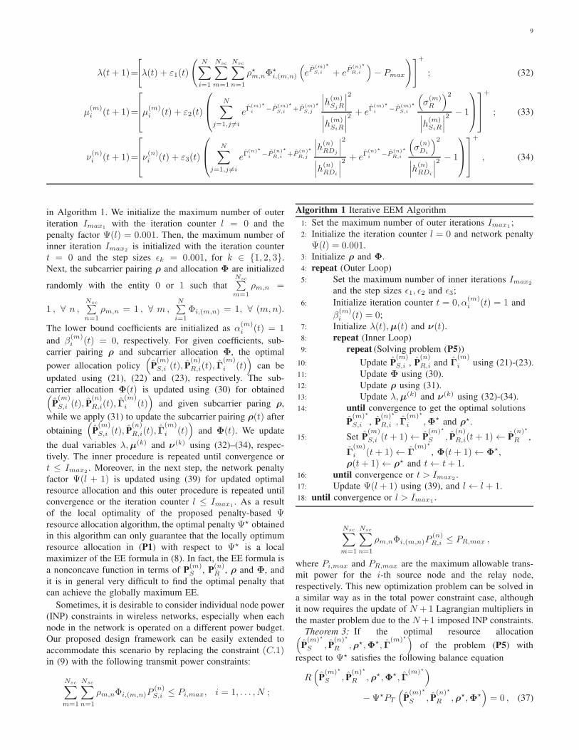
Algorithm 1 Iterative EEM Algorithm
1: Set the maximum number of outer iterations Imax1 ;
2: Initialize the iteration counter l = 0 and network penalty
Ψ(l) = 0.001.
3: Initialize ρ and Φ.
4: repeat (Outer Loop)
5: Set the maximum number of inner iterations Imax2
and the step sizes ǫ1, ǫ2 and ǫ3;
6: Initialize iteration counter t = 0, α(m)i (t) = 1 and
β(m)i (t) = 0;
7: Initialize λ(t),µ(t) and ν(t).8: repeat (Inner Loop)
9: repeat (Solving problem (P5))
10: Update P(m)
S,i , P(n)
R,i and Γ(m)
i using (21)-(23).
11: Update Φ using (30).
12: Update ρ using (31).
13: Update λ,µ(k) and ν(k) using (32)-(34).
14: until convergence to get the optimal solutions
P(m)⋆
S,i , P(n)⋆
R,i , Γ(m)⋆
i ,Φ⋆ and ρ⋆.
15: Set P(m)
S,i (t+ 1)← P(m)⋆
S , P(n)
R,i(t+ 1)← P(n)⋆
R ,
Γ(m)
i (t+ 1)← Γ(m)⋆
, Φ(t+ 1)← Φ⋆,
ρ(t+ 1)← ρ⋆ and t← t+ 1.
16: until convergence or t > Imax2 .
17: Update Ψ(l+ 1) using (39), and l ← l + 1.
18: until convergence or l > Imax1 .
Nsc∑
m=1
Nsc∑
n=1
ρm,nΦi,(m,n)P(n)R,i ≤ PR,max ,
where Pi,max and PR,max are the maximum allowable trans-
mit power for the i-th source node and the relay node,
respectively. This new optimization problem can be solved in
a similar way as in the total power constraint case, although
it now requires the update of N +1 Lagrangian multipliers in
the master problem due to the N+1 imposed INP constraints.
Theorem 3: If the optimal resource allocation(
P(m)⋆
S , P(n)⋆
R ,ρ⋆,Φ⋆, Γ(m)⋆
)
of the problem (P5) with
respect to Ψ⋆ satisfies the following balance equation
R(
P(m)⋆
S , P(n)⋆
R ,ρ⋆,Φ⋆, Γ(m)⋆
)
−Ψ⋆PT
(
P(m)⋆
S , P(n)⋆
R ,ρ⋆,Φ⋆)
= 0 , (37)

10
then Ψ⋆ will be the optimal penalty for the resources allo-
cated2.
Proof: The proof of Theorem 3 is similar to the proof in
[6, Appendix D].
D. Update procedure for penalty factor Ψ
The penalty factor Ψ is defined as
Ψ =FLB
(
ρ,Φ, Γ(m)
,α(m),β(m))
N∑
i=1
Nsc∑
m=1
Nsc∑
n=1ρm,nΦi,(m,n)
(
eP(m)S,i + eP
(n)R,i
)
+ Pc
, (38)
It is now important to find out what will be the optimal
penalty for resource allocation and also how can we update
it. To tackle these two problems, we furthermore propose the
following two theorems, respectively.
Theorem 4: If the penalty factor is updated for the (l+1)-th iteration for the local maximizer of the problem (P3) i.e.,(
P(m)⋆
S (l), P(n)⋆
R (l),ρ⋆(l),Φ⋆(l), Γ(m)⋆
(l))
, for the penalty
Ψ(l) in the l-th iteration as
Ψ(l + 1) =R(
P(m)⋆
S (l), P(n)⋆
R (l),ρ⋆(l),Φ⋆(l), Γ(m)⋆
(l))
PT
(
P(m)⋆
S (l), P(n)⋆
R (l),ρ⋆(l),Φ⋆(l)) ,
(39)
then the penalty Ψ(l) is monotonically increased with l.
Proof: The proof of Theorem 4 is similar to the proof in
[6, Appendix E].
Theorem 5: The optimal penalty factor can be obtained at
the convergence point i.e. Ψ⋆ = liml→∞
Ψ(l) satisfies the balance
equation.
Proof: The proof of Theorem 5 is similar to the proof in
[6, Appendix F].
V. ANALYSIS OF OPTIMAL RESOURCE ALLOCATION
POLICIES FOR TWO-USER CASES
To get more insight into the obtained optimal solutions in
the previous section, we consider the two-user cases in the
following two regimes:
1) Interference-Dominated (ID) Regime: We assume that
the network operates at very high SNR, consequently equiv-
alent noise power at the relay and the destination nodes
is diminutive as compared to the interference powers i.e.,
P(m)S,1
∣∣∣h
(m)S2R
∣∣∣
2
≫(
σ(m)R
)2
, P(m)S,2
∣∣∣h
(m)S2R
∣∣∣
2
≫(
σ(m)R
)2
and
P(n)R,1
∣∣∣h
(n)RD1
∣∣∣
2
≫(
σ(n)D2
)2
, P(n)R,2
∣∣∣h
(n)RD2
∣∣∣
2
≫(
σ(n)D1
)2
, respec-
tively.
Case 1: When P(m)S,1
∣∣∣h
(m)S2R
∣∣∣
2
≫(
σ(m)R
)2
, P(m)S,2
∣∣∣h
(m)S2R
∣∣∣
2
≫
2Since the original optimization problem is nonconvex, thus the optimalsolution obtained for (P5) works as a local maximizer here.
(
σ(m)R
)2
, the optimal power for both users are given as
eP(m)2
S,1 = µ(m)1 eΓ
(m)1 +P
(m)S,2
∣∣∣h
(m)S2R
∣∣∣
2
∣∣∣h
(m)S1R
∣∣∣
2
×
(Ψ + λ) ρ⋆m,nΦ
⋆2,(m,n) + µ
(m)2 eΓ
(m)2 −P
(m)S,2
∣∣∣h
(m)S1R
∣∣∣
2
∣∣∣h
(m)S2R
∣∣∣
2
−1
;
(40)
eP(m)2
S,2 = µ(m)2 eΓ
(m)2 +P
(m)S,1
∣∣∣h
(m)S1R
∣∣∣
2
∣∣∣h
(m)S2R
∣∣∣
2
×
(Ψ + λ) ρ⋆m,nΦ
⋆2,(m,n) + µ
(m)1 eΓ
(m)1 −P
(m)S,1
∣∣∣h
(m)S2R
∣∣∣
2
∣∣∣h
(m)S1R
∣∣∣
2
−1
,
(41)
In practice, the transmit power should be different from zero
for all nodes. Since the m-th subcarrier is allocated to the first
source node, the power allocated on the m-th subcarrier by
the second source node is almost close to zero. Thus, it can
be observed in (40) and (41) that the source node allocates
less transmit power on the m-th subcarrier if it has better
subcarrier gain among all allocated subcarriers to it in order
to improve the EE, whereas in case of without subcarrier
pairing and power allocation, the power allocation policy for
the first(second) source node is affected by the second(first)
source channel gain.
Case 2: For P(n)R,1
∣∣∣h
(n)RD1
∣∣∣
2
≫(
σ(n)D2
)2
, P(n)R,2
∣∣∣h
(n)RD2
∣∣∣
2
≫(
σ(n)D1
)2
, we can get the optimal power for both users similar
to (40) and (41) as follows:
eP(m)2
S,1 =
µ(m)1
eΓ
(m)1 +P
(m)S,2
∣∣∣h
(m)S2R
∣∣∣
2
∣∣∣h
(m)S1R
∣∣∣
2 + eΓ(m)1
(
σ(m)R
)2
∣∣∣h
(m)S1R
∣∣∣
2
(Ψ + λ) ρ⋆m,nΦ⋆1,(m,n) + µ
(m)2
e
Γ(m)2 −P
(m)S,2
∣∣∣h
(m)S1R
∣∣∣
2
∣∣∣h
(m)S2R
∣∣∣
2
; (42)
eP(n)2
S,2 =
µ(n)2
eΓ
(m)2 +P
(m)S,1
∣∣∣h
(m)S1R
∣∣∣
2
∣∣∣h
(m)S2R
∣∣∣
2 + eΓ(m)2
(
σ(m)R
)2
∣∣∣h
(m)S2R
∣∣∣
2
(Ψ + λ) ρ⋆m,nΦ⋆2,(m,n) + µ
(m)1
e
Γ(m)1 −P
(m)S,1
∣∣∣h
(m)S2R
∣∣∣
2
∣∣∣h
(m)S1R
∣∣∣
2
, (43)
2) Noise-Dominated (ND) Regime: When the network op-
erates under a very low SNR, then the disturbances produced
by the noise at the relay and the destination nodes become
11
significantly high as compared to the interference generated
at the respective nodes.
• Relay-Noise Dominated (RND) Regime: In this regime,
the relay noise is very high as compared to the interference
produced at the relay node i.e., P(m)S,1
∣∣∣h
(m)S1R
∣∣∣
2
≪(
σ(m)R
)2
and P(m)S,2
∣∣∣h
(m)S2R
∣∣∣
2
≪(
σ(m)R
)2
, respectively. The ratio of the
optimal power of first user to the second user is given as
eP(m)⋆
2
S,1
eP(m)⋆
2
S,2
=µ(m)1 eΓ
(m)1 Φ⋆
2,(m,n)
µ(m)2 eΓ
(m)2 Φ∗
1,(m,n)
∣∣∣h
(m)S2R
∣∣∣
2
∣∣∣h
(m)S1R
∣∣∣
2 , (44)
This result reveals a channel-reversal power allocation policy,
in which a user with a lower SR channel gain is allocated
higher transmit power.
• Destination-Noise Dominated (DND) Regime: The desti-
nation noise is very high in this regime as compared to the
interference i.e., P(n)R,2
∣∣∣h
(n)RD2
∣∣∣
2
≪(
σ(n)D1
)2
and P(n)R,1
∣∣∣h
(n)RD1
∣∣∣
2
≪(
σ(n)D2
)2
, respectively. The optimal power for both users can
be obtained similar to (42) and (43).
VI. SUBOPTIMAL EE RESOURCE ALLOCATION
ALGORITHM
For a large number of Nsc or N , the computational com-
plexity of the proposed EEM algorithm in Section IV becomes
very high. Thus, we propose a low-complexity suboptimal
EE algorithm whose performance is close to that of the
EEM algorithm. The suboptimal EE algorithm is sketched as
follows:
A. Step 1: Optimal Subcarrier Allocation for Fixed Power
Allocation
First, we equally distribute the available transmit powers
over all the subcarriers among the source and the relay nodes:
P(m)S,1 = P
(m)S,2 = . . . = P
(m)S,N =
Pmax
2NNsc, ∀m ; (45)
P(n)R,1 = P
(n)R,2 = . . . = P
(n)R,N =
Pmax
2NNsc, ∀n , (46)
Using (2) and (4), we find SINR for each user pair and then
take minimum SINR in order to balance the EE of the SR and
RD links as
Ξi,(m,n) = minγ(m)SRi
, γ(n)RDi ; (47)
Next we update the subcarrier allocation matrix as follows:
Φi,(m,n) =
1, for i = argmaxi Ξi,(m,n) ;
0, otherwise(48)
B. Step 2: Optimal Subcarrier Pairing for Given Subcarrier
Allocation
In the second step, we arrange the SR subcarriers in a
descending order according to their channel gains, and the RDsubcarriers are also ordered in the same way. Then, we match
the corresponding subcarriers with each other in sequence.
If the m-th subcarrier of the SR link is paired with the n-
th subcarrier of the RD link, we set ρm,n = 1; otherwise
ρm,n = 0.
C. Step 3: Optimal Power Allocation for Given Subcarrier
Pairing and Allocation
In the last step, for given subcarrier allocation and pairing
matrices Φ and ρ, we allocate the power to each source and
the relay nodes using (24) and (25).
VII. COMPLEXITY ANALYSIS
In this section, we perform an exhaustive complexity anal-
ysis to get a better insight into the complexity reduced by the
EEM and suboptimal EEM algorithms.
• EEM Algorithm: First the complexity of the EEM
algorithm is analyzed as follows. To find the optimal power
allocation of (P5) for N user pairs with Nsc subcarriers in
each hop, we need to solve NN2sc subproblems. The optimal
power allocation solution(
P(m)⋆
S,i , P(n)⋆R,i
)
can be found using
the exhaustive search (ES) approach which searches over
P(m)S,i and P
(n)R,i under assumption that each takes discrete
values [29]. Therefore, K denotes the number of power
levels that can be taken by each of P(m)S,i and P
(n)R,i. Each
subcarrier pairing ρm,n is allocated to a particular user pair
and each maximization in (30) has a complexity of O (N),hence the total complexity for subcarrier allocation becomes
O(NN2
sc
). Furthermore, the Hungarian method is used to
determine optimal subcarrier pairing in (31) with a complexity
of O(N3
sc
). The complexity of updating a dual variable is
O ((2N)) (for example, = 2 if the ellipsoid method is
used [26]). Therefore, the total complexity for updating dual
variables is O (3(2N)). Let us suppose if the dual objective
function g (λ,µ,ν) and the penalty factor Ψ converge in
Z and L iterations, respectively, the total complexity for
EEM algorithm is O(3(2N)N2
scZL(N(K3 + 2
)+Nsc
)),
whereas with equal subcarrier power allocation (ESPA),
the total complexity of EEM algorithm becomes
O(5(2N)N2
scZL(N(K3 + 4
)+Nsc
)).
• Without subcarrier allocation and pairing (WSAP): In
this algorithm only power is allocated optimally without
considering the subcarrier allocation and pairing, respectively.
Thus we update the power and the dual variables with com-
plexity of O(NN2
scZ(K3 + 1
))and O (3(2N)), respec-
tively. Thus the total complexity for this algorithm becomes
O(3(2N)NLN2
sc
(K3 + 1
)).
• Suboptimal Algorithm: The implementation of the subcar-
rier allocation in step 1 as stated in (48) requires a complexity
of O (2NNsc), whereas the subcarrier pairing in step 2
has a complexity of O (2Nsc). Further, the power allocation
in the last step adds a complexity of O(Nsc
(K3 + 1
))
and the total complexity for updating dual variables is
O (3(2N)). If the dual objective function g (λ,µ,ν) and
the penalty factor Ψ converge in Z and L iterations, respec-
tively, then the the suboptimal algorithm has a complexity of
O(3(2N)NscZL
(2N +K3 + 3
)).
• Exhaustive search (ES): As a benchmark, we compare
the complexity of the proposed algorithms with the exhaus-
tive search (ES) algorithm, which gives the optimal solution
after searching over all variables. However, the complexity
of ES increases very quickly as the size of the problem
increases. Therefore, ES search is typically used when the
12
TABLE ICOMPLEXITY ANALYSIS FOR DIFFERENT ALGORITHMS
Complexity Comparison
Algorithm Complexity
EEM O(
3(2N)N2scZL
(
N(
K3 + 2)
+Nsc
))
Suboptimal EEM O(
3(2N)NscZL(
2N +K3 + 3))
ESPA O(
5(2N)N2scZL
(
N(
K3 + 4)
+Nsc
))
WSAP O(
3(2N)NLN2sc
(
K3 + 1))
ES O(
3(2N)ZLNNsc!(
K3 + 1))
problem size is limited. The complexity of ES can be given
by O(3(2N)ZLNNsc!
(K3 + 1
)). The complexity of the
proposed algorithms and ES is summarized in Table I.
VIII. SIMULATION RESULTS
In this section, we evaluate the performance of the proposed
energy efficient resource allocation algorithms through com-
puter simulations. The path loss model stated by 131.1+42.8×log10(d) dB (d: distance in km) is adopted in our simulations
[30]. Moreover, the log-normal shadowing ∼ lnN (0, 8dB)and independently and identically distributed (i.i.d.) Rayleigh
fading effects ∼ CN (0, 1) for all links in the considered
framework are taken into consideration, respectively. It is
assumed that the circuit and processing power dissipation
per antenna at each node is 14 dBm, respectively [6]. The
subcarrier spacing and thermal noise density are given by 12kHz and −174 dBm/Hz, respectively. The maximum number
of inner and outer iterations Imax1 and Imax2 for proposed
algorithms are set as 10, and the convergence tolerance value
is 10−5. The constant step sizes ǫ1, ǫ2, and ǫ3 are used in
Algorithm with value 0.01. The penalty factor Ψ that shows a
tradeoff between the EE and the SE is Ψ = 0.001. We define
a distance ratio as rd = dSR/(dSR + dRD), where dSR and
dRD are used to present the distance from all source nodes
to the relay node and from the relay node to all destination
nodes, respectively. The ES algorithm which gives the optimal
solution of the considered problem, the proposed EEM algo-
rithm without (w/o) subcarrier pairing and allocation (SPA)
and the spectral efficiency maximization (SEM) algorithm are
also implemented for performance comparison.
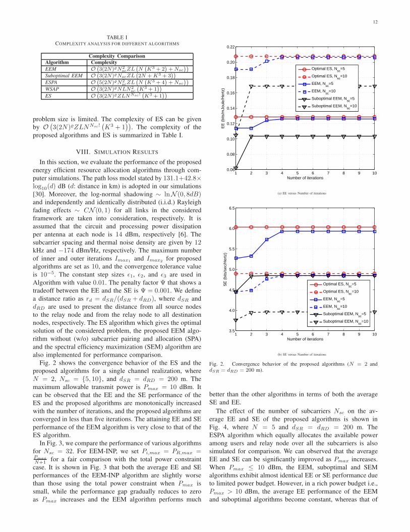
Fig. 2 shows the convergence behavior of the ES and the
proposed algorithms for a single channel realization, where
N = 2, Nsc = 5, 10, and dSR = dRD = 200 m. The
maximum allowable transmit power is Pmax = 10 dBm. It
can be observed that the EE and the SE performance of the
ES and the proposed algorithms are monotonically increased
with the number of iterations, and the proposed algorithms are
converged in less than five iterations. The attaining EE and SE
performance of the EEM algorithm is very close to that of the
ES algorithm.
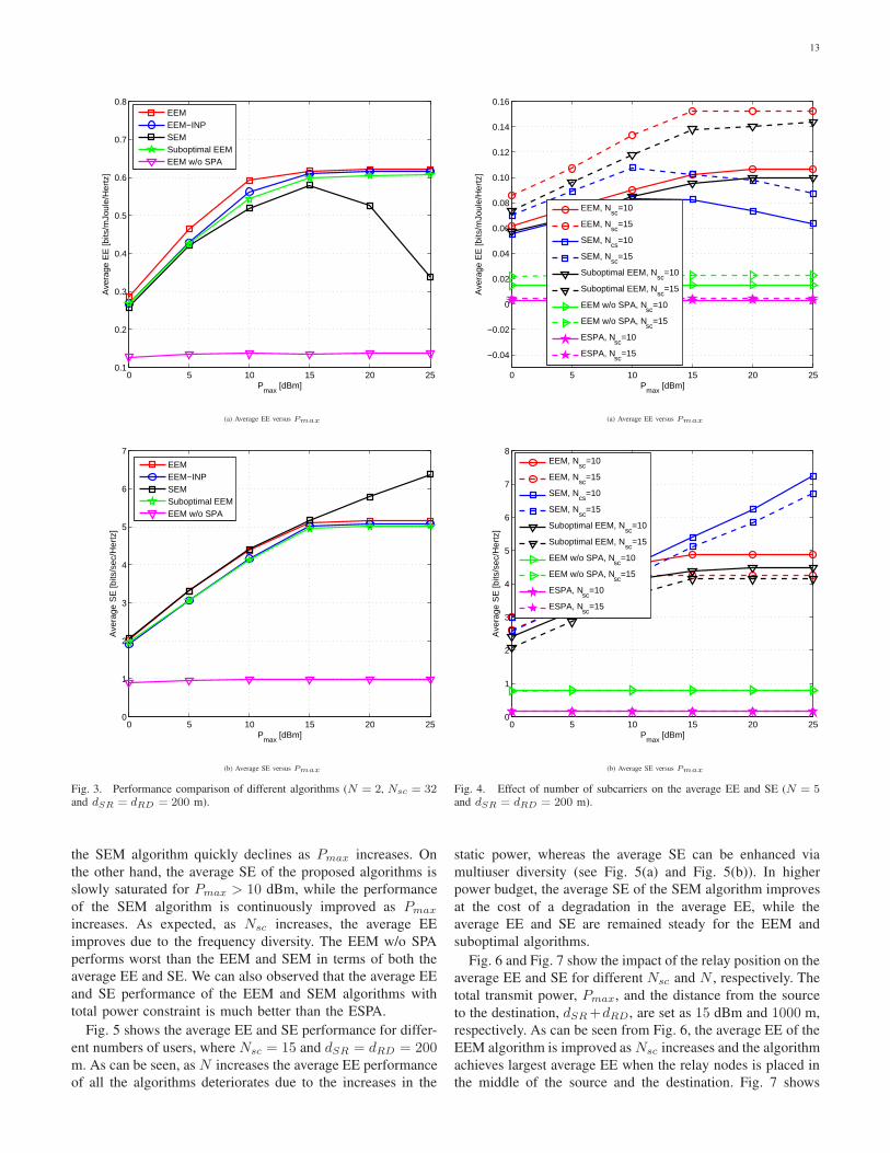
In Fig. 3, we compare the performance of various algorithms
for Nsc = 32. For EEM-INP, we set Pi,max = PR,max =Pmax
N+1 for a fair comparison with the total power constraint
case. It is shown in Fig. 3 that both the average EE and SE
performances of the EEM-INP algorithm are slightly worse
than those using the total power constraint when Pmax is
small, while the performance gap gradually reduces to zero
as Pmax increases and the EEM algorithm performs much
1 2 3 4 5 6 7 8 9 100.06
0.08
0.10
0.12
0.14
0.16
0.18
0.20
0.22
Number of iterations
EE
(bi
ts/m
Joul
e/H
ertz
)
Optimal ES, Nsc
=5
Optimal ES, Nsc
=10
EEM, Nsc
=5
EEM, Nsc
=10
Suboptimal EEM, Nsc
=5
Suboptimal EEM, Nsc
=10
(a) EE versus Number of iterations
1 2 3 4 5 6 7 8 9 103.5
4.0
4.5
5.0
5.5
6.0
6.5
Number of iterations
SE
(bi
ts/s
ec/H
ertz
)
Optimal ES, Nsc
=5
Optimal ES, Nsc
=10
EEM, Nsc
=5
EEM, Nsc
=10
Suboptimal EEM, Nsc
=5
Suboptimal EEM, Nsc
=10
(b) SE versus Number of iterations
Fig. 2. Convergence behavior of the proposed algorithms (N = 2 anddSR = dRD = 200 m).
better than the other algorithms in terms of both the average
SE and EE.
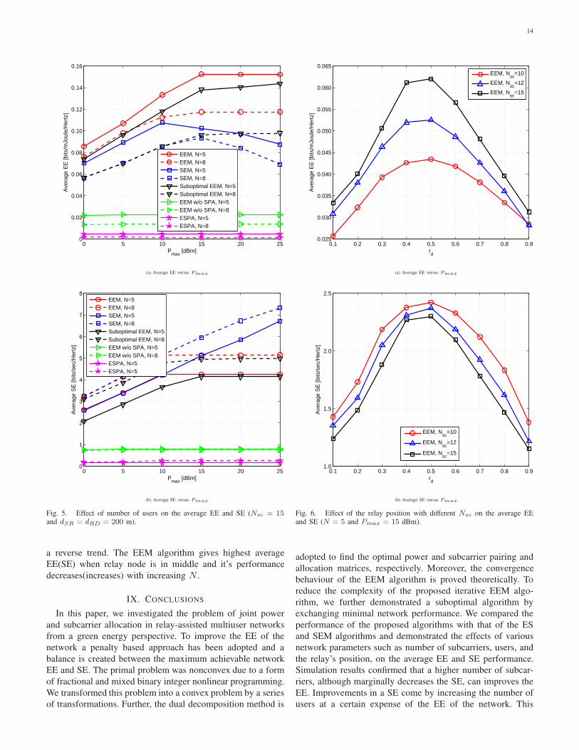
The effect of the number of subcarriers Nsc on the av-
erage EE and SE of the proposed algorithms is shown in
Fig. 4, where N = 5 and dSR = dRD = 200 m. The
ESPA algorithm which equally allocates the available power
among users and relay node over all the subcarriers is also
simulated for comparison. We can observed that the average
EE and SE can be significantly improved as Pmax increases.
When Pmax ≤ 10 dBm, the EEM, suboptimal and SEM
algorithms exhibit almost identical EE or SE performance due
to limited power budget. However, in a rich power budget i.e.,
Pmax > 10 dBm, the average EE performance of the EEM
and suboptimal algorithms become constant, whereas that of
13
0 5 10 15 20 250.1
0.2
0.3
0.4
0.5
0.6
0.7
0.8
Pmax
[dBm]
Ave
rage
EE
[bits
/mJo
ule/
Her
tz]
EEMEEM−INPSEMSuboptimal EEMEEM w/o SPA
(a) Average EE versus Pmax
0 5 10 15 20 250
1
2
3
4
5
6
7
Pmax
[dBm]
Ave
rage
SE
[bits
/sec
/Her
tz]
EEMEEM−INPSEMSuboptimal EEMEEM w/o SPA
(b) Average SE versus Pmax
Fig. 3. Performance comparison of different algorithms (N = 2, Nsc = 32and dSR = dRD = 200 m).
the SEM algorithm quickly declines as Pmax increases. On
the other hand, the average SE of the proposed algorithms is
slowly saturated for Pmax > 10 dBm, while the performance
of the SEM algorithm is continuously improved as Pmax
increases. As expected, as Nsc increases, the average EE
improves due to the frequency diversity. The EEM w/o SPA
performs worst than the EEM and SEM in terms of both the
average EE and SE. We can also observed that the average EE
and SE performance of the EEM and SEM algorithms with
total power constraint is much better than the ESPA.
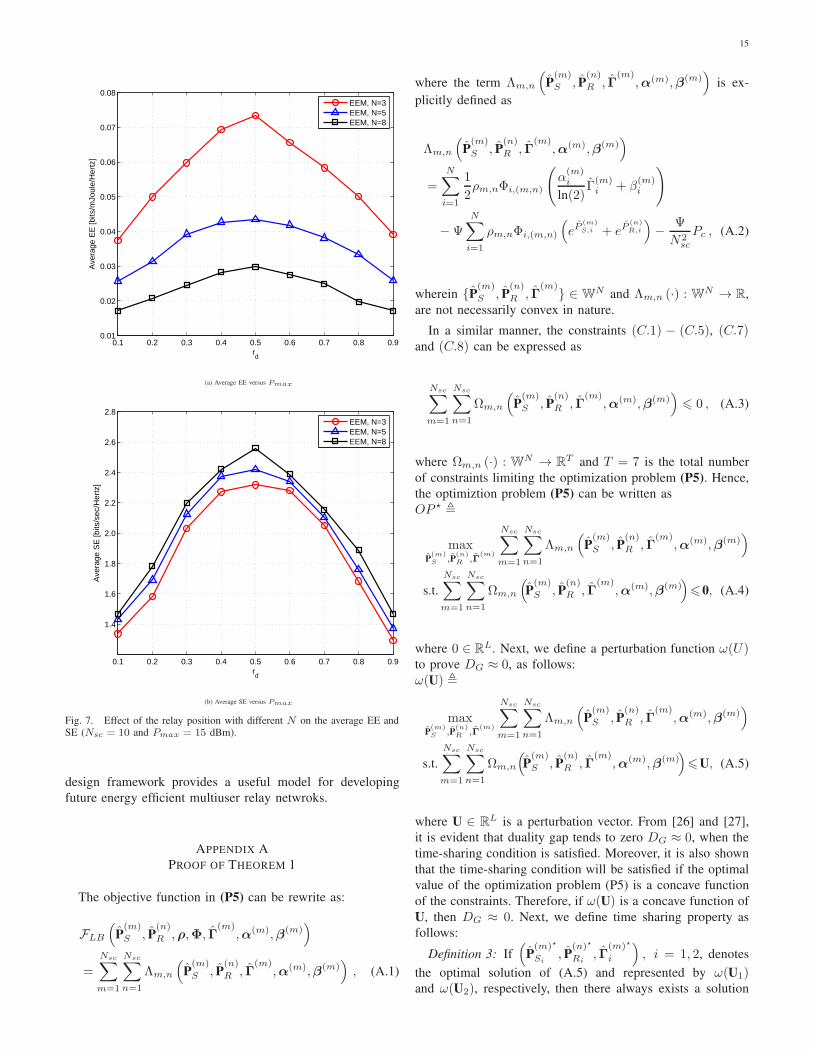
Fig. 5 shows the average EE and SE performance for differ-
ent numbers of users, where Nsc = 15 and dSR = dRD = 200m. As can be seen, as N increases the average EE performance
of all the algorithms deteriorates due to the increases in the
0 5 10 15 20 25
−0.04
−0.02
0
0.02
0.04
0.06
0.08
0.10
0.12
0.14
0.16
Pmax
[dBm]
Ave
rage
EE
[bits
/mJo
ule/
Her
tz]
EEM, Nsc
=10
EEM, Nsc
=15
SEM, Ncs
=10
SEM, Nsc
=15
Suboptimal EEM, Nsc
=10
Suboptimal EEM, Nsc
=15
EEM w/o SPA, Nsc
=10
EEM w/o SPA, Nsc
=15
ESPA, Nsc
=10
ESPA, Nsc
=15
(a) Average EE versus Pmax
0 5 10 15 20 250
1
2
3
4
5
6
7
8
Pmax
[dBm]
Ave
rage
SE
[bits
/sec
/Her
tz]
EEM, N
sc=10
EEM, Nsc
=15
SEM, Ncs
=10
SEM, Nsc
=15
Suboptimal EEM, Nsc
=10
Suboptimal EEM, Nsc
=15
EEM w/o SPA, Nsc
=10
EEM w/o SPA, Nsc
=15
ESPA, Nsc
=10
ESPA, Nsc
=15
(b) Average SE versus Pmax
Fig. 4. Effect of number of subcarriers on the average EE and SE (N = 5and dSR = dRD = 200 m).
static power, whereas the average SE can be enhanced via
multiuser diversity (see Fig. 5(a) and Fig. 5(b)). In higher
power budget, the average SE of the SEM algorithm improves
at the cost of a degradation in the average EE, while the
average EE and SE are remained steady for the EEM and
suboptimal algorithms.
Fig. 6 and Fig. 7 show the impact of the relay position on the
average EE and SE for different Nsc and N , respectively. The
total transmit power, Pmax, and the distance from the source
to the destination, dSR+dRD, are set as 15 dBm and 1000 m,
respectively. As can be seen from Fig. 6, the average EE of the
EEM algorithm is improved as Nsc increases and the algorithm
achieves largest average EE when the relay nodes is placed in
the middle of the source and the destination. Fig. 7 shows
14
0 5 10 15 20 250
0.02
0.04
0.06
0.08
0.10
0.12
0.14
0.16
Pmax
[dBm]
Ave
rage
EE
[bits
/mJo
ule/
Her
tz]
EEM, N=5EEM, N=8SEM, N=5SEM, N=8Suboptimal EEM, N=5Suboptimal EEM, N=8EEM w/o SPA, N=5EEM w/o SPA, N=8ESPA, N=5ESPA, N=8
(a) Average EE versus Pmax
0 5 10 15 20 250
1
2
3
4
5
6
7
8
Pmax
[dBm]
Ave
rage
SE
[bits
/sec
/Her
tz]
EEM, N=5EEM, N=8SEM, N=5SEM, N=8Suboptimal EEM, N=5Suboptimal EEM, N=8EEM w/o SPA, N=5EEM w/o SPA, N=8ESPA, N=5ESPA, N=5
(b) Average SE versus Pmax
Fig. 5. Effect of number of users on the average EE and SE (Nsc = 15and dSR = dRD = 200 m).
a reverse trend. The EEM algorithm gives highest average
EE(SE) when relay node is in middle and it’s performance
decreases(increases) with increasing N .
IX. CONCLUSIONS
In this paper, we investigated the problem of joint power
and subcarrier allocation in relay-assisted multiuser networks
from a green energy perspective. To improve the EE of the
network a penalty based approach has been adopted and a
balance is created between the maximum achievable network
EE and SE. The primal problem was nonconvex due to a form
of fractional and mixed binary integer nonlinear programming.
We transformed this problem into a convex problem by a series
of transformations. Further, the dual decomposition method is
0.1 0.2 0.3 0.4 0.5 0.6 0.7 0.8 0.90.025
0.030
0.035
0.040
0.045
0.050
0.055
0.060
0.065
rd
Ave
rage
EE
[bits
/mJo
ule/
Her
tz]
EEM, N
sc=10
EEM, Nsc
=12
EEM, Nsc
=15
(a) Average EE versus Pmax
0.1 0.2 0.3 0.4 0.5 0.6 0.7 0.8 0.91.0
1.5
2.0
2.5
rd
Ave
rage
SE
[bits
/sec
/Her
tz]
EEM, Nsc
=10
EEM, Nsc
=12
EEM, Nsc
=15
(b) Average SE versus Pmax
Fig. 6. Effect of the relay position with different Nsc on the average EEand SE (N = 5 and Pmax = 15 dBm).
adopted to find the optimal power and subcarrier pairing and
allocation matrices, respectively. Moreover, the convergence
behaviour of the EEM algorithm is proved theoretically. To
reduce the complexity of the proposed iterative EEM algo-
rithm, we further demonstrated a suboptimal algorithm by
exchanging minimal network performance. We compared the
performance of the proposed algorithms with that of the ES
and SEM algorithms and demonstrated the effects of various
network parameters such as number of subcarriers, users, and
the relay’s position, on the average EE and SE performance.
Simulation results confirmed that a higher number of subcar-
riers, although marginally decreases the SE, can improves the
EE. Improvements in a SE come by increasing the number of
users at a certain expense of the EE of the network. This
15
0.1 0.2 0.3 0.4 0.5 0.6 0.7 0.8 0.90.01
0.02
0.03
0.04
0.05
0.06
0.07
0.08
rd
Ave
rage
EE
[bits
/mJo
ule/
Her
tz]
EEM, N=3EEM, N=5EEM, N=8
(a) Average EE versus Pmax
0.1 0.2 0.3 0.4 0.5 0.6 0.7 0.8 0.9
1.4
1.6
1.8
2.0
2.2
2.4
2.6
2.8
rd
Ave
rage
SE
[bits
/sec
/Her
tz]
EEM, N=3EEM, N=5EEM, N=8
(b) Average SE versus Pmax
Fig. 7. Effect of the relay position with different N on the average EE andSE (Nsc = 10 and Pmax = 15 dBm).
design framework provides a useful model for developing
future energy efficient multiuser relay netwroks.
APPENDIX A
PROOF OF THEOREM 1
The objective function in (P5) can be rewrite as:
FLB
(
P(m)
S , P(n)
R ,ρ,Φ, Γ(m)
,α(m),β(m))
=
Nsc∑
m=1
Nsc∑
n=1
Λm,n
(
P(m)
S , P(n)
R , Γ(m)
,α(m),β(m))
, (A.1)
where the term Λm,n
(
P(m)
S , P(n)
R , Γ(m)
,α(m),β(m))
is ex-
plicitly defined as
Λm,n
(
P(m)
S , P(n)
R , Γ(m)
,α(m),β(m))
=
N∑
i=1
1
2ρm,nΦi,(m,n)
(
α(m)i
ln(2)Γ(m)i + β
(m)i
)
−Ψ
N∑
i=1
ρm,nΦi,(m,n)
(
eP(m)S,i + eP
(n)R,i
)
−Ψ
N2sc
Pc , (A.2)
wherein P(m)
S , P(n)
R , Γ(m) ∈ W
N and Λm,n (·) : WN → R,
are not necessarily convex in nature.
In a similar manner, the constraints (C.1) − (C.5), (C.7)and (C.8) can be expressed as
Nsc∑
m=1
Nsc∑
n=1
Ωm,n
(
P(m)
S , P(n)
R , Γ(m)
,α(m),β(m))
6 0 , (A.3)
where Ωm,n (·) : WN → RT and T = 7 is the total number
of constraints limiting the optimization problem (P5). Hence,
the optimiztion problem (P5) can be written as
OP ⋆ ,
maxP(m)S ,P
(n)R ,Γ
(m)
Nsc∑
m=1
Nsc∑
n=1
Λm,n
(
P(m)
S , P(n)
R , Γ(m)
,α(m),β(m))
s.t.
Nsc∑
m=1
Nsc∑
n=1
Ωm,n
(
P(m)
S , P(n)
R , Γ(m)
,α(m),β(m))
60, (A.4)
where 0 ∈ RL. Next, we define a perturbation function ω(U)
to prove DG ≈ 0, as follows:
ω(U) ,
maxP(m)S ,P
(n)R ,Γ
(m)
Nsc∑
m=1
Nsc∑
n=1
Λm,n
(
P(m)
S , P(n)
R , Γ(m)
,α(m),β(m))
s.t.
Nsc∑
m=1
Nsc∑
n=1
Ωm,n
(
P(m)
S , P(n)
R , Γ(m)
,α(m),β(m))
6U, (A.5)
where U ∈ RL is a perturbation vector. From [26] and [27],
it is evident that duality gap tends to zero DG ≈ 0, when the
time-sharing condition is satisfied. Moreover, it is also shown
that the time-sharing condition will be satisfied if the optimal
value of the optimization problem (P5) is a concave function
of the constraints. Therefore, if ω(U) is a concave function of
U, then DG ≈ 0. Next, we define time sharing property as
follows:
Definition 3: If(
P(m)⋆
Si, P
(n)⋆
Ri, Γ
(m)⋆
i
)
, i = 1, 2, denotes
the optimal solution of (A.5) and represented by ω(U1)and ω(U2), respectively, then there always exists a solution
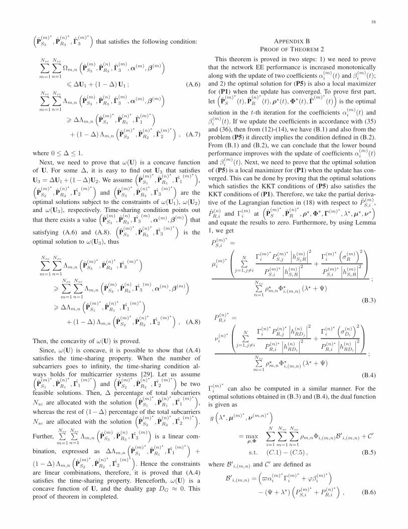
16
(
P(m)⋆
S3, P
(n)⋆
R3, Γ
(m)⋆
3
)
that satisfies the following condition:
Nsc∑
m=1
Nsc∑
n=1
Ωm,n
(
P(m)
S3, P
(n)
R3, Γ
(m)
3 ,α(m),β(m))
6 ∆U1 + (1−∆)U1 ; (A.6)
Nsc∑
m=1
Nsc∑
n=1
Λm,n
(
P(m)
S3, P
(n)
R3, Γ
(m)
3 ,α(m),β(m))
> ∆Λm,n
(
P(m)⋆
S1, P
(n)⋆
R1, Γ
(m)⋆
1
)
+ (1−∆)Λm,n
(
P(m)⋆
S2, P
(n)⋆
R2, Γ
(m)⋆
2
)
, (A.7)
where 0 ≤ ∆ ≤ 1.
Next, we need to prove that ω(U) is a concave function
of U. For some ∆, it is easy to find out U3 that satisfies
U3 = ∆U1+(1−∆)U2. We assume(
P(m)⋆
S1, P
(n)⋆
R1, Γ1
(m)⋆)
,(
P(m)⋆
S2, P
(n)⋆
R2, Γ2
(m)⋆)
and(
P(m)⋆
S3, P
(n)⋆
R3, Γ3
(m)⋆)
are the
optimal solutions subject to the constraints of ω(U1), ω(U2)and ω(U3), respectively. Time-sharing condition points out
that there exists a value(
P(m)
S3, P
(n)
R3, Γ3
(m),α(m),β(m)
)
that
satisfying (A.6) and (A.8).(
P(m)⋆
S3, P
(n)⋆
R3, Γ3
(m)⋆)
is the
optimal solution to ω(U3), thus
Nsc∑
m=1
Nsc∑
n=1
Λm,n
(
P(m)⋆
S3, P
(n)⋆
R3, Γ3
(m)⋆)
>
Nsc∑
m=1
Nsc∑
n=1
Λm,n
(
P(m)
S3, P
(n)
R3, Γ3
(m),α(m),β(m)
)
> ∆Λm,n
(
P(m)⋆
S1, P
(n)⋆
R1, Γ1
(m)⋆)
+ (1−∆)Λm,n
(
P(m)⋆
S2, P
(n)⋆
R2, Γ2
(m)⋆)
, (A.8)
Then, the concavity of ω(U) is proved.
Since, ω(U) is concave, it is possible to show that (A.4)
satisfies the time-sharing property. When the number of
subcarriers goes to infinity, the time-sharing condition al-
ways holds for multicarrier systems [29]. Let us assume(
P(m)⋆
S1, P
(n)⋆
R1, Γ1
(m)⋆)
and(
P(m)⋆
S2, P
(n)⋆
R2, Γ2
(m)⋆)
be two
feasible solutions. Then, ∆ percentage of total subcarriers
Nsc are allocated with the solution(
P(m)⋆
S1, P
(n)⋆
R1, Γ1
(m)⋆)
,
whereas the rest of (1−∆) percentage of the total subcarriers
Nsc are allocated with the solution(
P(m)⋆
S2, P
(n)⋆
R2, Γ2
(m)⋆)
.
Further,Nsc∑
m=1
Nsc∑
n=1Λm,n
(
P(m)
S3, P
(n)
R3, Γ3
(m))
is a linear com-
bination, expressed as ∆Λm,n
(
P(m)⋆
S1, P
(n)⋆
R1, Γ1
(m)⋆)
+
(1−∆)Λm,n
(
P(m)⋆
S2, P
(n)⋆
R2, Γ2
(m)⋆)
. Hence the constraints
are linear combinations, therefore, it is proved that (A.4)
satisfies the time-sharing property. Henceforth, ω(U) is a
concave function of U, and the duality gap DG ≈ 0. This
proof of theorem in completed.
APPENDIX B
PROOF OF THEOREM 2
This theorem is proved in two steps: 1) we need to prove
that the network EE performance is increased monotonically
along with the update of two coefficients α(m)i (t) and β
(m)i (t);
and 2) the optimal solution for (P5) is also a local maximizer
for (P1) when the update has converged. To prove first part,
let(
P(m)⋆
S (t), P(n)⋆
R (t),ρ⋆(t),Φ⋆(t), Γ(m)⋆
(t))
is the optimal
solution in the t-th iteration for the coefficients α(m)i (t) and
β(m)i (t). If we update the coefficients in accordance with (35)
and (36), then from (12)-(14), we have (B.1) and also from the
problem (P5) it directly implies the condition defined in (B.2).
From (B.1) and (B.2), we can conclude that the lower bound
performance improves with the update of coefficients α(m)i (t)
and β(m)i (t). Next, we need to prove that the optimal solution
of (P5) is a local maximizer for (P1) when the update has con-
verged. This can be done by proving that the optimal solutions
which satisfies the KKT conditions of (P5) also satisfies the
KKT conditions of (P1). Therefore, we take the partial deriva-
tive of the Lagrangian function in (18) with respect to P(m)S,i ,
P(n)R,i and Γ
(m)i at
(
P(m)⋆
S , P(n)⋆
R ,ρ⋆,Φ⋆,Γ(m)⋆ , λ⋆,µ⋆,ν⋆)
and equate the results to zero. Furthermore, by using Lemma
1, we get
P(m)⋆
S,i =
µ(m)⋆
i
N∑
j=1,j 6=i
Γ(m)⋆
i P(m)⋆
S,j
∣∣∣h
(m)SjR
∣∣∣
2
P(m)⋆
S,i
∣∣∣h
(m)SiR
∣∣∣
2 +Γ(m)⋆
i
(
σ(m)R
)2
P(m)⋆
S,i
∣∣∣h
(m)SiR
∣∣∣
2
Nsc∑
n=1ρ⋆m,nΦ
⋆i,(m,n) (λ
⋆ +Ψ)
;
(B.3)
P(n)⋆
R,i =
ν(n)⋆
i
N∑
j=1,j 6=i
Γ(n)⋆
i P(n)⋆
R,j
∣∣∣h
(n)RDj
∣∣∣
2
P(n)⋆
R,i
∣∣∣h
(n)RDi
∣∣∣
2 +Γ(n)⋆
i
(
σ(n)Di
)2
P(n)⋆
R,i
∣∣∣h
(n)RDi
∣∣∣
2
Nsc∑
m=1ρ⋆m,nΦ
⋆i,(m,n) (λ
⋆ +Ψ)
;
(B.4)
Γ(m)⋆
i can also be computed in a similar manner. For the
optimal solutions obtained in (B.3) and (B.4), the dual function
is given as
g(
λ⋆,µ(m)⋆ ,ν(m,n)⋆)
= maxρ,Φ
N∑
i=1
Nsc∑
m=1
Nsc∑
n=1
ρm,nΦi,(m,n)B′i,(m,n) + C
′
s.t. (C.1) − (C.5) , (B.5)
where B′i,(m,n) and C′ are defined as
B′i,(m,n) =
(
α(m)⋆
i Γ(m)⋆
i + ϕβ(m)⋆
i
)
− (Ψ + λ⋆)(
P(m)⋆
S,i + P(n)⋆
R,i
)
, (B.6)
17
FLB
(
P(m)⋆
S (t), P(n)⋆
R (t),ρ⋆(t),Φ⋆(t),Γ(m)⋆(t),α(m)(t),β(m)(t))
≤ F(
P(m)⋆
S (t), P(n)⋆
R (t),ρ⋆(t),Φ⋆(t),Γ(m)⋆(t))
= FLB
(
P(m)⋆
S (t), P(n)⋆
R (t),ρ⋆(t),Φ⋆(t),Γ(m)⋆(t), α(m)i (t+ 1), β
(m)i (t+ 1)
)
; (B.1)
FLB
(
P(m)⋆
S (t), P(n)⋆
R (t),ρ⋆(t),Φ⋆(t),Γ(m)⋆(t), α(m)i (t+ 1), β
(m)i (t+ 1)
)
(B.2)
≤ FLB
(
P(m)⋆
S (t+ 1), P(n)⋆
R (t+ 1),ρ⋆(t+ 1),Φ⋆(t+ 1),Γ(m)⋆(t+ 1), α(m)i (t+ 1), β
(m)i (t+ 1)
)
,
C′ = −ΨPc + λ⋆Pmax
−N∑
i=1
Nsc∑
k=1
µ(k)⋆
i
N∑
j=1,j 6=i
(
Γ(k)⋆
i + P(k)⋆
S,j
) ∣∣∣h
(k)SjR
∣∣∣
2
P(k)⋆
S,i
∣∣∣h
(k)SiR
∣∣∣
2
+Γ(k)⋆
i
(
σ(k)R
)2
P(k)⋆
S,i
∣∣∣h
(k)SiR
∣∣∣
2 + 1
−N∑
i=1
Nsc∑
k=1
ν(k)⋆
i
N∑
j=1,j 6=i
(
Γ(k)⋆
i + P(k)⋆
R,j
) ∣∣∣h
(k)RDj
∣∣∣
2
P(k)⋆
R,i
∣∣∣h
(k)RDi
∣∣∣
2
+Γ(k)⋆
i
(
σ(k)Di
)2
P(k)⋆
R,i
∣∣∣h
(k)RDi
∣∣∣
2 + 1
, (B.7)
Similar to (29) the optimal subcarrier allocation is determined
for a given subcarrier pairing as
Φ⋆i,(m,n) =
1, for i = argmaxi B′i,(m,n) ,
0, otherwise(B.8)
and the optimal subcarrier pairing matrix for obtained power
and subcarrier allocation can be found similar to (31) where
B′ is defined as
B′ =
B′i⋆,(1,1) · · · B′
i⋆,(1,K)
.... . .
...
B′i⋆,(K,1) · · · B′
i⋆,(K,K)
(B.9)
Moreover, the optimal solution of (P1) can be derived from the
KKT conditions that the partial derivatives of the Lagrangian
function of the problem (P1) with respect to P(m)S,i and P
(n)R,i
are identical to (B.3) and (B.4), respectively. This is also true
for the subcarrier pairing and allocation matrix. Hence, the
theorem is proved.
REFERENCES
[1] J. N. Laneman, D. N. C. Tse, and G. W. Wornell, “Cooperative diversity inwireless networks: efficient protocols and outage behavior,” IEEE Trans.
Inf. Theory, vol. 50, no. 1, pp. 3062-3080, Dec. 2004.
[2] Y. Chen, S. Zhang, S. Xu, and G. Li, “Fundamental trade-offs on greenwireless networks,” IEEE Commun. Mag., vol. 49, no. 6, pp. 30-37, Jun.2011.
[3] C. Han, T. Harrold, S. Armour, I. Krikidis, S. Videv, P. Grant, H. Haas,J. Thompson, I. Ku, C.-X. Wang, T.A. Le, M. Nakhai, J. Zhang, andL. Hanzo, “Green radio: Radio techniques to enable energy-efficientnetworks,” IEEE Commun. Mag., vol. 49, no. 6, pp. 46-54, Jun. 2011.
[4] D. Gunduz, A. Yener, A. Goldsmith, and H. V. Poor, “The multiway relaychannel,” IEEE Trans. Inf. Theory, vol. 59, no. 1, pp. 51-63, Jan. 2013.
[5] O. Arnold, F. Richter, G. Fettweis, and O. Blume, “Power consumptionmodeling of different base station types in heterogeneous cellular net-works,” in IEEE Proc. FNMS’10, pp. 1-8, Jun. 2010.
[6] K. Singh and M.-L. Ku, “Toward green power allocation in relay-assistedmultiuser networks: a pricing-based approach,” IEEE Trans. Wireless
Commun., vol. 14, no. 5, pp. 2470- 2486, May 2015.
[7] L. Vandendorpe, R. Duran, J. Louveaux, and A. Zaidi, “ Power allocationfor OFDM transmission with DF relaying,” in Proc. IEEE ICC’08, pp.3795-3800, May 2008.
[8] L. Vandendorpe, J. Louveaux, O. Oguz and A. Zaidi, “Rate-optimizedpower allocation for DF-relayed OFDM transmission under sum andindividual power constraints,” EURASIP J. Wireless Commun. and Netw.,,pp. 1-11, Jun. 2009.
[9] W. Y. Li, W. Wang, J. Kong, and M. Peng, “Subcarrier pairing for amplify-and-forward and decode-and-forward OFDM relay links,” IEEE Commun.
Lett., vol. 13, no. 4, pp. 209-211, Apr. 2009.
[10] W. Dang, M. Tao, H. Mu, and J. Huang, “Subcarrier-based resourceallocation for cooperative multi-relay OFDM systems,” IEEE Trans.
Wireless Commun., vol. 9, no. 5, pp. 1640-1649, May 2010.
[11] S. Senthuran, A. Anpalagan, and O. Das, “Cooperative subcarrier andpower allocation for a two-hop decode-and-forward OFCDM based relaynetwork,” IEEE Trans. Wireless Commun., vol. 8, no. 9, pp. 4797-4805,Sep. 2009.
[12] C.-N. Hsu, H.-J. Su, and P.H. Lin “Joint subcarrier pairing and powerallocation for OFDM transmission with decode-and-forward relaying,”IEEE Trans. Singal Process., vol. 59, no. 1, pp. 399-414, Jan. 2011.
[13] X. Zhang, X. Shen, and L.-L. Xie, “Joint subcarrier and power allocationfor cooperative communications in LTE-advanced networks,” IEEE Trans.
Wireless Commun., vol. 13, no. 2, pp. 658-668, Feb. 2014.
[14] G. A. S. Sindhu, F. G. Gao, W. Chen, and A. Nallanathan, “A jointresource allocation scheme for multiuser two-way relay networks,” IEEE
Trans. Commun., vol. 59, no. 11, pp. 2970-2975, Nov. 2011.
[15] W. Li, J. Lei, T. Wang, C. Xiong, and J. Wei, “Dynamic optimization forresource allocation in relay-aided OFDMA systems under multiservice,”IEEE Trans. Veh. Technol., vol. 65, no. 3, pp. 1303-1313, Mar. 2016.
[16] C. C. Zarakovitis, Q. Ni, and J. Spiliotis, “Energy efficient green wirelesscommunication systems with imperfect CSI and data outage,” IEEE J. Sel.
Areas Commun., vol. pp, no.99, Aug. 2016.
[17] C. C. Zarakovitis and Q. Ni, “Maximizing energy efficiency in multiusermulticarrier broadband wireless systems: convex relaxation and globaloptimization techniques,” IEEE Trans. Veh. Technol., vol. 65, no. 7, pp.5275-5286, Jul. 2016.
[18] C. Xiong, G. Y. Li, S. Zhang, Y. Chen, and S. Xu, “Energy-efficient re-source allocation in OFDMA networks,” in Proc. IEEE GLOBECOM’11,pp. 1-5, Dec. 2011.
[19] K. Singh, M.-L. Ku, and J.-C. Lin, “Power control for achieving energy-efficient multiuser two-way balancing relay networks,” in Proc. IEEE
ICASSP’14, pp. 2749-2753, May 2014.
[20] J. Papandriopoulos and J. S. Evans, “SCALE: a low-complexity dis-tributed protocol for spectrum balancing in multiuser DSL networks,”IEEE Trans. Inf. Theory, vol. 55, no. 8, pp. 3711-3724, Aug. 2009.

18
[21] P. Monti, S. Tombaz, L. Wosinska, and J. Zander, “Mobile backhaulin heterogeneous network deployments: Technology options and powerconsumption, in Proc. IEEE ICTON’12, pp. 1-7, Jul. 2012.
[22] J. Jang and K. B. Lee, “Transmit power adaptation for multiuser OFDMsystems,” IEEE J. Sel. Areas Commun., vol. 21, no. 2, pp. 171-178, Feb2003.
[23] S. Boyd and L. Vandenberghe, “Convex optimization,” Cambridge, U.K.:Cambridge Univ. Press, 2004.
[24] W. Dinkelbach, “On nonlinear fractional programming,” Management
Science, vol. 13, no. 7, pp. 492-498, Mar. 1967.[25] Y. Li, W. Wang, J. Kong, W. Hong, X. Zhang and M. Peng, “Power
allocation and subcarrier pairing in OFDM-based relaying networks,” inProc. IEEE ICC’08, pp. 2602-2606, May 2008.
[26] W. Yu and R. Lui, “Dual methods for nonconvex spectrum optimizationof multicarrier systems,” IEEE Trans. Commun., vol. 54, no. 7, pp. 1310-1322, Jul. 2006.
[27] K. Seong, M. Mohseni, and J. M. Cioffi, “Optimal resource allocationfor OFDMA downlink systems,” in Proc. IEEE ISIT’06, pp. 1394-1398,Jul. 2006.
[28] H. W. Kuhn, “The Hungarian method for the assignment problem,” in 50
Years of Integer Programming 1958-2008., Springer Berlin Heidelberg,pp. 29-47, 2010.
[29] Y. U. Jang, E. R. Jeong, and Y. H. Lee, “A two-step approach to powerallocation for OFDM signals over two-way amplify-and-forward relay,”IEEE Trans. Signal Process., vol. 58, no. 4, pp. 2426-2430, Apr. 2010.
[30] 3GPP, TR 36.819 (V9.0.0), “Further advancement for E-UTRA physicallayer aspects (Release 9),” Mar. 2010.
Keshav Singh (S’12, M’16) received the degreeof Master of Technology (with first-class hon-ors) in Computer Science from Devi Ahilya Vish-wavidyalaya, Indore, India, in 2006, the M.Sc. inInformation & Telecommunications Technologiesfrom Athens Information Technology, Greece, in2009, and the Ph.D. degree in Communication En-gineering from National Central University, Taiwan,in 2015. Since 2016, he has been with Institutefor Digital Communications, School of Engineering,University of Edinburgh, where he is currently a
Postdoctoral Research Associate. He is a memeber of IEEE. He also hasserved as a Technical Program Committee Member for numerous IEEEconferences. His current research interests are in the areas of green com-munications, resource allocation, full-duplex radio, cooperative and energyharvesting networks, multiple-input multiple-output (MIMO) systems, andoptimization of radio access.
Ankit Gupta received the Bachelor of Technology(B.Tech) degree in Electronics and CommunicationEngineering from Guru Gobind Singh IndraprasthaUniversity, Delhi, India, in 2014. He is currentlywith Aricent Technologies Limited (Holdings), Gu-rugram, India. His current research interests in-clude 5G, cooperative communications, multiple-input multiple-output (MIMO) networks and opti-mization methods in signal processing and commu-nications.
Tharmalingam Ratnarajah (A’96-M’05-SM’05) iscurrently with the Institute for Digital Communica-tions, University of Edinburgh, Edinburgh, UK, asa Professor in Digital Communications and SignalProcessing and the Head of Institute for DigitalCommunications. His research interests include sig-nal processing and information theoretic aspects of5G and beyond wireless networks, full-duplex radio,mmWave communications, random matrices theory,interference alignment, statistical and array signalprocessing and quantum information theory. He has
published over 300 publications in these areas and holds four U.S. patents.He is currently the coordinator of the FP7 project ADEL (3.7Me) in thearea of licensed shared access for 5G wireless networks. Previously, hewas the coordinator of the FP7 project HARP (3.2Me) in the area ofhighly distributed MIMO and FP7 Future and Emerging Technologies projectsHIATUS (2.7Me) in the area of interference alignment and CROWN (2.3Me)in the area of cognitive radio networks. Dr Ratnarajah is a Fellow of HigherEducation Academy (FHEA), U.K., and an associate editor of the IEEETransactions on Signal Processing.


![National Institute of Technology, Hamirpur2018/08/15 · National Institute of Technology Hamirpur [I-I-PI] Chairman Member Member Member Member Member Member Member 201 1/ 65 Dr.R.L.Sharma,](https://img.pdfslide.us/doc/110x75/5f297161e38dfc50516f3156/national-institute-of-technology-20180815-national-institute-of-technology.jpg)