Embed Size (px)
Citation preview

Vol. 04 / Issue. 02 / 2015
Accelerate Innovation with CFD & Thermal CharacterizationEDGE
mentor.com/mechanical
General Electric Winner of Inaugural Don Miller Award Page 21
Bertrandt Group Lighting the Way Page 16
Thales Corporate EngineeringElectronics Thermal Design Page 13
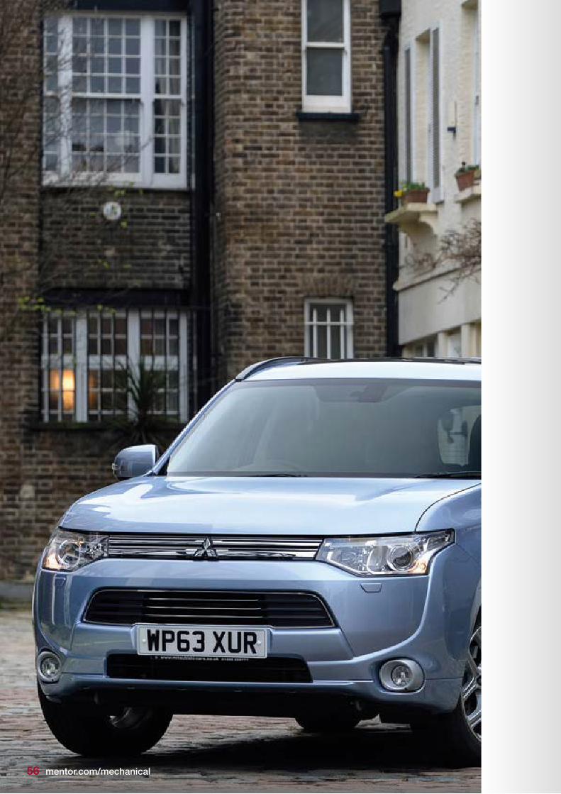
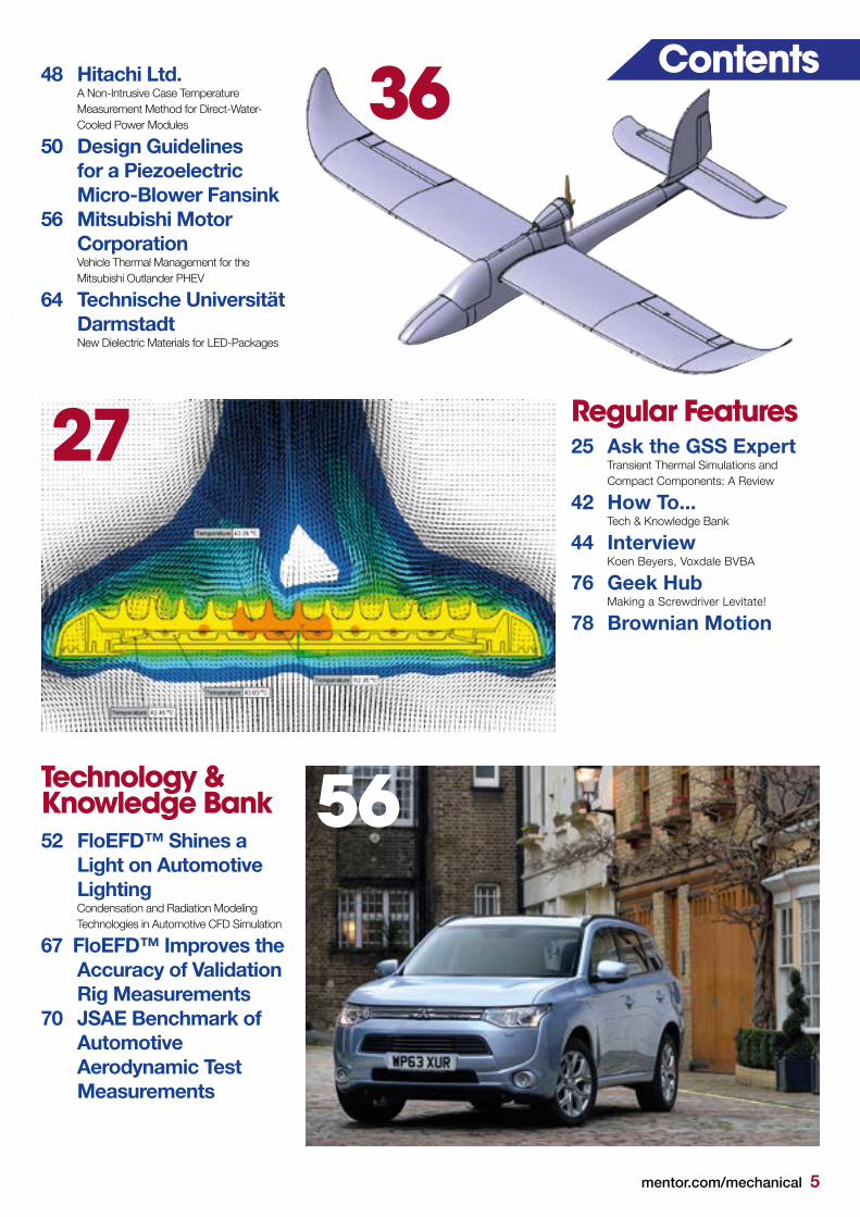
Mitsubishi Vehicle Thermal Management Studies Page 56

2 mentor.com/mechanical
It’s Easy…
1. Like our ‘Mechanical Analysis Division’ Facebook page2. Upload an image of your work, with a short description by the 14th Dec 2015 and you could win lunch on us and be featured in Engineering Edge.

mentor.com/mechanical 3
PerspectiveVol. 04, Issue. 02
Greetings readers! It is with great pleasure that I take the time here to acknowledge my colleague, Prof. Márta Rencz, who recently won the prestigious ASME Allan Kraus Thermal Management Award “…for eminent achievement in thermal management of electronic systems”. This recognizes her work in the field of thermal characterization of electronics (page 9). Márta is an inspiration to many of us in the Mechanical Analysis Division. While we are talking MicReD, it’s worth acknowledging the work of researchers at the Korean Institute of Science and Technology who have published a report in the prestigious Nature Magazine in August entitled
“Three-Dimensional Porous Copper-Graphene Heterostructures with Durability and High Heat Dissipation Performance” (page 11). They have created a brand new graphene-based material with dramatically enhanced thermal properties for the electronics industry employing our T3Ster® hardware to demonstrate its thermal performance for LED cooling.
The inaugural Don Miller Award for Excellence in Thermo-Fluid System Simulation has been won by Andrea Tradii and Stefano Rossin of GE Oil & Gas (page 21), with their 1D multi-physics presentation entitled "Experimental Validation of Steam Turbine Control Oil Actuation Systems Transient Behavior". This is a practical and pragmatic application of engineering simulation tools to a real-world problem. Our new product releases, Flowmaster® V7.9.4 and FloTHERM® V11.0 are rounded up on pages 7 and 6 respectively. The wealth of customer stories in this edition of Engineering Edge, have a real automotive and ground transportation flavor. Bertrandt Group in Germany have produced a great article on how they use FloEFD™ for automotive headlight design (page 16); while my colleague Chris Watson has a fascinating article on how FloEFD 15.0 models automotive lights for both of the two most challenging scenarios of condensation and icing conditions (page 52). And Robert Bosch highlights the use of FloEFD in component simulation (page 33). From Asia Pacific, Mitsubishi Motors Corporation, Japan, describe some great electric vehicle thermal management system simulation studies with Flowmaster (page 56), while Hitachi Ltd. (page 48) have used the MicReD T3ster® for non-intrusive thermal studies of liquid cooled IGBTs for electric vehicles. The report on the automotive external aerodynamics blind benchmark run by JSAE (page 70) in Japan demonstrates how good FloEFD is out-of-the-box relative to traditional CFD codes. And our friends at Voxdale in Belgium use FloEFD for a student open-wheel sports car competition. (page 45)
Check out NIAR’s work on UAV aerodynamics using FloEFD (pages 36). ECS in Silicon Valley continue to use FloTHERM XT and T3Ster to teardown tablet computers (page 30) whereas Vestel Streetlight Terminal designs streetlights in Turkey using FloEFD (pages 27). Two University stories from TU Darmstadt (page 64) in Germany and IWATE University (page 50) in Japan - both using FloTHERM for cutting edge projects.
As always, I like to see the imagination of our engineers being applied to our tools. Mike Gruetzmacher, our new FloEFD Technical Marketing Engineer, has had some fun simulating the levitation of screwdrivers and ping-pong balls in FloEFD (page 76). John Wilson’s How to Guide (page 42) covers heatsink optimization with FloTHERM and Command Center. Richard Merrett and Steve Streater use our unique 1D-3D CFD capabilities with FloEFD and Flowmaster to verify experimental test rig measurement locations (page 67). And last, but not least, Koen Beyers from Voxdale, a long-time “power user” of FloEFD offers his thoughts on future trends of CAD-embedded CFD in our regular industry thought-leader Interview on page 44. Finally, I urge you all to submit your entries for the Don Miller Award for Excellence in Thermo-Fluid System Simulation. For more information visit our website: http://bit.ly/1SLhZUX
Mentor Graphics CorporationPury Hill Business Park,
The Maltings,Towcester, NN12 7TB,
United KingdomTel: +44 (0)1327 306000
email: [email protected]
Editor:Keith Hanna
Managing Editor:Natasha Antunes
Copy Editor:Jane Wade
Contributors: Byron Blackmore, Mike Croegeart, Mike
Gruetzmacher, Keith Hanna, Andrey Ivanov, Boris Marovic, Richard Merrett, John Murray, John Parry,
Sarah Pyle, Akbar Sahrapour, Svetlana Shtilkind, Steve Streater, Chris Watson, John Wilson
With special thanks to:Bertrandt Group,
Electronic Cooling Solutions Inc., EnginSoft Nordic,
Flow Design Bureau AS, General Electric Nuovo Pignone S.p.A,
General Electric Oil & Gas,Hitachi Ltd.,
Mitsubishi Motors Corporation,National Institute for Aviation Research,
National University Corporation Iwate University, Technische Universität Darmstadt,
Thales Corporate Engineering, United Automotive Electronics, Systems Co. Ltd.,
Vestel Electronic - LED Lighting, and Voxdale BVBA
©2015 Mentor Graphics Corporation, all rights reserved. This document contains
information that is proprietary to Mentor Graphics Corporation and may be duplicated
in whole or in part by the original recipient for internal business purposes only, provided that this entire notice appears in all copies. In
accepting this document, the recipient agrees to make every reasonable effort to prevent
unauthorized use of this information. All trademarks mentioned in this publication are
the trademarks of their respective owners.
Vol. 04 / Issue. 02 / 2015
Accelerate Innovation with CFD & Thermal CharacterizationEDGE
mentor.com/mechanical
General Electric Winner of Inaugural Don Miller Award Page 21
Bertrandt Group Lighting the Way Page 16
Thales Corporate EngineeringElectronics Thermal Design Page 13
Mitsubishi Vehicle Thermal Management Studies Page 56
Roland Feldhinkel, General ManagerMechanical Analysis Division, Mentor Graphics
It’s Easy…
1. Like our ‘Mechanical Analysis Division’ Facebook page2. Upload an image of your work, with a short description by the 14th Dec 2015 and you could win lunch on us and be featured in Engineering Edge.
4 mentor.com/mechanical
News6 New Release: FloTHERM® V11.07 New Release: Flowmaster® V7.9.48 Mentor Graphics’ New Technology Partner 9 Awards10 2015 Don Miller Award for Excellence11 High Thermal Performance Copper-Graphene Heterostructures
16
21
Engineering Edge13 Thales Corporate Engineering A Step Further in Thermal Modeling of Electronic Components
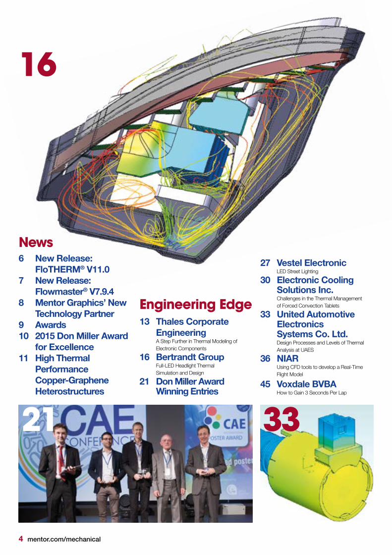
16 Bertrandt Group Full-LED Headlight Thermal Simulation and Design
21 Don Miller Award Winning Entries
27 Vestel Electronic LED Street Lighting
30 Electronic Cooling Solutions Inc. Challenges in the Thermal Management of Forced Convection Tablets
33 United Automotive Electronics Systems Co. Ltd. Design Processes and Levels of Thermal Analysis at UAES
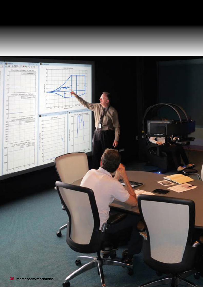
36 NIAR Using CFD tools to develop a Real-Time Flight Model
45 Voxdale BVBA How to Gain 3 Seconds Per Lap
33
mentor.com/mechanical 5
Contents
Technology & Knowledge Bank52 FloEFD™ Shines a Light on Automotive Lighting Condensation and Radiation Modeling Technologies in Automotive CFD Simulation
67 FloEFD™ Improves the Accuracy of Validation Rig Measurements70 JSAE Benchmark of Automotive Aerodynamic Test Measurements
Regular Features25 Ask the GSS Expert Transient Thermal Simulations and Compact Components: A Review
42 How To... Tech & Knowledge Bank
44 Interview Koen Beyers, Voxdale BVBA
76 Geek Hub Making a Screwdriver Levitate!
78 Brownian Motion
36
27
56
48 Hitachi Ltd. A Non-Intrusive Case Temperature Measurement Method for Direct-Water- Cooled Power Modules
50 Design Guidelines for a Piezoelectric Micro-Blower Fansink56 Mitsubishi Motor Corporation Vehicle Thermal Management for the Mitsubishi Outlander PHEV
64 Technische Universität Darmstadt New Dielectric Materials for LED-Packages

6 mentor.com/mechanical
Figure 3. Localized grid spaces defined for a heatsink and a component
New Release: FloTHERM® V11.0
he release of FloTHERM V11.0 in July 2015 brought both functional and productivity gains to the user community. As always, features
were developed based on direct customer feedback and aimed at streamlining workflows and increasing productivity to allow a broader range of applications to be handled more efficiently than ever.
FloTHERM V11.0 introduces a new capability to solve for electrical potential, current density, and the resultant 3D Joule heating distribution concurrently with temperature. The user applies electrical boundary conditions (voltages, currents, and electrical resistivities) and the FloTHERM solver does the rest. Users can now consider additional applications, including power distribution on PCB nets and bus bar design. Figure 1 shows typical results from a power distribution net model, displaying current flow vectors and the temperature distribution throughout the net.
Within the release, the FloMCAD Bridge module was completely reimplemented as part of the ongoing user interface update program. The new window includes 64-bit support, a model node tree, and a responsive graphics area enabling fully featured MCAD assemblies to be handled with ease.
The FloMCAD Bridge voxelization feature (which converts any MCAD part into a cuboid arrangement) has been re-engineered to be bigger, faster, and smarter.
• Bigger: The limit on maximum voxelization resolution has been removed. Models can be created with whatever granularity is needed.
• Faster: A re-engineered approach to voxelization in V11.0 is 20x faster than the previous version
• Smarter: A voxelization mesh display allows full control over the voxelization process, and a novel approach in which all MCAD parts are voxelized on the same mesh guarantees that coincident MCAD faces will be air-tight when converted into FloTHERM objects.
The grid system in FloTHERM has always been a core strength of the software, and
it’s even better in FloTHERM V11.0. The basics remain unchanged. Users will still work with the robust, instantaneous, object based gridding system, always viewing the grid as the model is constructed. New in this release, is the ability to overlap localized grid spaces. This removes a historical restriction and further streamlines the gridding workflow. Users can define object grid settings as usual, and simply ‘Localize’ the object grid as needed, further boosting productivity with the tool.
Automation technology also jumps forward in FloTHERM V11.0. FloSCRIPT support has been extended to fully support the new FloMCAD Bridge module enabling MCAD design import, simplification, and translation to be reduced to a single click. Further, FloSCRIPT playback can be initiated from a command line or external software. Spreadsheet macros are easily developed to drive FloTHERM externally, with full model build, solving, and tabular results extraction
supported. Massive productivity gains can be realized with this new technology, and Mentor Graphics Global Support and Services have the expertise to develop customized automation solutions for you.
T
Figure 1. Results from a PDN analysis in FloTHERM V11.0
Figure 2. Original MCAD geometry, Voxelization Mesh Display in FloMCAD Bridge and the FloTHERM model that results.
mentor.com/mechanical 7
New Release:Flowmaster® V7.9.4
ith the release of Flowmaster V7.9.4, announced in July 2015, Mentor Graphics continues the product line’s
30 plus year history of product development and advancement. Flowmaster V7.9.4 is a combination of significant functionality and user experience enhancements that will be of value to all Flowmaster users. As always, a significant number of the developments are based on suggestions originating from customer input. In addition to the software developments, Flowmaster has continued to add several additional validation and verification reports, available on SupportNet to anyone who has an active SupportNet account.
This release of Flowmaster features significant enhancements to some of its unique analysis capabilities including Multi-arm Tank, Auto-vaporization, and reservoir results reporting. Additionally, Flowmaster can now perform hydrodynamic force calculations and export those results to leading pipe stress softwares. User experience is V7.9.4 has seen a particular focus on usability. To this end a number of individual improvements have been included which, taken together, significantly improve the user experience. Details of Flowmaster product enhancements:
Multi-Arm Tank The multi-arm tank component has undergone a significant revision at V7.9.4. The energy balance of the model has been revised with two distinct heat transfer models being implemented: polytropic and full heat transfer. These changes improve the heat balance of the system and thereby improve convergence and the stability of the model.
Auto-Vaporization The implementation of this important feature was reviewed to ensure that it was being applied both consistently and in a manner that wouldn’t compromise the stability of user systems.
• The artificial clipping of static pressure should it drop below zero was removed, although users will be warned if this does occur.
• The calculation of nodal static pressure – which will be compared with vapor
W pressure – will now be based upon the maximum dynamic pressure connected to the node. This approach is consistently applied should a cavity form.
• Auto-vaporization has been applied to the transition components, for which vapor pressure is now an optional data input.
• Turning on auto-vaporisation at nodes connected to pressure specifying components creates a stability issue. It will no longer be possible to do this in V7.9.4.
New Result Features In order to complement a broader body of work on the reservoir components, it is now possible to integrate volumetric flow rate from the tabular data result report. The pressure at tank bottom is also reported for; two and three armed reservoirs, the closed system sump blowdown, and expansion tanks.
NIST REFPROP AccessThe NIST REFPROP fluid property database underpins Flowmaster’s compressible and two phase solvers. At V7.9.4 more information is now available regarding the accuracy of curves and surfaces generated in Flowmaster by the user. Should a generated fluid fall outside the tolerances specified, the user will be warned at the point of saving the fluid and advice given on how to improve the situation will be displayed.
Hydrodynamic Force Calculation and ExportIt is now possible to calculate the hydrodynamic force generated by a fluid transient event and export the resulting force time history to both SST CAEPIPE and Integraph® CAESAR II®. The hydrodynamic force result feature is available for the following components when run as part of an incompressible transient, priming, or restart simulation:
• All cylindrical elastic pipes;
• Check and relief valve;
• Control Valves; and
• Transitions.
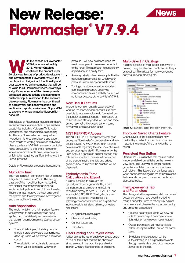
Filter Catalog and Project Views A filter box at the top of each view allows users to find all items that contain the character string entered in the box. It is possible to interact with any found entities at this point.
Multi-Select in Catalogs It is now possible to multi-select items within a catalog using the standard control or shift keys as required. This allows for more convenient copying, moving, deleting etc.
Improved Saved Charts FeatureCharts saved to the project tree are now marked by a distinct icon and modifications made to the format of the charts can be re-saved.
Persistent Run Button Users at V7.9.4 will notice that the run button is now available from all tabs on the network view pane. The user will no longer need to go to the simulation data tab in order to run a simulation. This feature is of particular value when considered alongside the re-usable chart feature and changes to the experiments tab discussed below.
The Experiments Tab and ParametersThe changes to the experiments tab and input/output parameters have been included to make it easier for users to modify key system parameters and observe the impact as quickly and smoothly as possible.
• Creating parameters: users will now be able to create output parameters via a right-click on any relevant result feature.
• Output parameters will now be visible below input parameters, but on the same pane.
• By default, the latest result will be auto-selected, but it is possible to cycle through results via a drop down network at the top of the tab.
Figure 1. Flowmaster catalog filtering in project view
News

8 mentor.com/mechanical
• The corresponding input parameter(s) will also be displayed.
• Transient time histories are now available from the experiments tab in the same manner found on the current data tab.
• The evaluated results from expression parameters are also displayed and can be distinguished from standard input parameters by the background color.
• Output parameter results are also now available from non-experiments simulations.
BookmarksA new “Bookmark” feature has been added to the charts window in Flowmaster. Bookmarks allow charts to be updated automatically on completion of a successful solution. It is possible to set references which persist in the plot, in order to allow users to compare the effects of a given modification with a benchmark or reference. It is possible to have more than one result feature per bookmark plot, and many bookmark plots concurrently in order to allow as a detailed picture of a network as is required to be created.
Bookmarks can be launched from the ‘Bookmarks’ button on any eligible chart
window. All the result features displayed on the chart at the time of opening the bookmarks dialog will appear in the left hand column of the resulting dialog. The column on the right will display all the eligible results. Note that ‘eligible’ in this context is with respect to the current chart: if transient results are shown, only transient results are eligible, the converse being true if the plot is showing steady state features versus (for example) pipe length. A reference result may be selected if the user wishes to make a comparison against a chosen baseline. Once activated, the bookmarked plot will update for all subsequent successful runs. The user may have many bookmark plots open concurrently.
Mentor Graphics’ New Technology Partner
ATADVANCE is a leading developer of software for engineering process integration, predictive modeling, intellectual
data analysis and multidisciplinary optimization.
This partnership grew from a successful joint implementation experience of DATADVANCE and the Mentor Graphics software tool, FloEFD™, to solve complex engineering problems of both companies’ clients. Joining the partner program, which provides access to a comprehensive suite of capabilities, followed an extensive review of FloEFD™ integration capabilities and pSeven – DATADVANCE’s flagship product.
The seamless integration between FloEFD and pSeven will allow users to perform complex parametric and trade-off studies, as well as
D solve multidisciplinary design optimization and uncertainty quantification problems using state-of-the-art data analysis and optimization algorithms. These capabilities significantly improve user experience of design team members in any industry, reducing design lead time while improving product efficiency, safety, and reliability, especially at the early design stages.
“Our synergies with our new technology partner DATADVANCE, will provide a fully integrated solution to ease the development of advanced products using our technologies. Our mutual development bases in Moscow permits optimal interaction, allowing us to serve our mutual customers with an optimum solution for productivity, faster time-to-market, and profitability,” stated Roland Feldhinkel, General Manager, Mentor Graphics Mechanical Analysis Division. More information: www.datadvance.net
Figure 2. Improved Variable Parameters viewing and Run Button Persistence
Figure 3. Bookmarks for Flowmaster plot window

mentor.com/mechanical 9
2015 Allan Kraus Award
Wally Rhines wins 2015 Phil Kaufman Award
FloEFD™ helps Novosanis Design Award Winning Colli-Pee™
he Allan Kraus Thermal Management Medal, established in 2009, recognizes individuals who have demonstrated outstanding
achievements in thermal management of electronic systems and their commitment to the field of thermal science and engineering.
This year the award goes to Professor Márta Rencz, Deputy Head of Department of Electron Devices, Budapest University of Technology & Economics.
he Electronic Design Automation Consortium and the IEEE Council on Electronic Design Automation, this month announced the winner
of the prestigious Phil Kaufman award. This year the accolade was awarded to Mentor Graphics Chairman and CEO, Dr. Walden (Wally) C Rhines, who was honored for his Leadership Role in Growing the EDA and IC Design Industries.
Dr. Rhines is considered a leading voice of the EDA industry to the larger high tech community, having presented hundreds of major keynote speeches
olli-Pee, the first void urine collection device, developed by Novosanis has received the IWT Innovation Award
in the Major Social Relevance category, awarded by The Agency for Innovation by Science and Technology.
Novosanis designs and develops medical devices for a variety of applications, ranging from injection
T
T
C
She received recognition for her work on the methodology of structure functions, based in situ and ex situ characterization of thermal interface materials and thermal characterization of semiconductor device packages. The work has become an industry standard for the measurement of junction-t o-case thermal resistance. Márta's work on structure function based test methods has led to the development of successful industrial products.
Marta Rencz is an electrical engineer with interests in the interdisciplinary aspects of electronics. She started to investigate the thermal issues in microelectronics over 20 years ago. She was co-founder and CEO of
and articles related to the semiconductor, electronic design and EDA industries.He has always maintained a neutral stance, focusing on issues that benefit the entire industry. He has also chaired the EDA Consortium for five two-year terms, growing the organization into an effective forum to address industry-wide issues.
Dr. Rhines served as a member of the Board of the Semiconductor Research Corporation (SRC). “As an SRC Board member, Dr. Rhines acted as the key communications link between the EDA industry and EDA users in the semiconductor and embedded systems industry,” says Dr. Georges G. E. Gielen, professor at Katholieke Universiteit Leuven. “He also provided motivational insights for students, professors and researchers into how
MicReD Ltd., acquired by Mentor Graphics in 2008. Under her guidance this company developed T3ster®, the first thermal transient tester, whose evaluation methodology is based on the structure function technology. This methodology has become the industry standard, and is now used by the electronics industry for the thermal qualification of packages.
Marta Rencz’s latest invention was the combination of thermal transient testing with structure function analysis and reliability testing based on active power cycling which allows continuous, non-destructive monitoring of the degradation process of power semiconductor devices.
EDA is impacting and changing the world.”
“Dr. Rhines has taken the high ground when speaking for the EDA industry and maintained a separation between industry positions and the specific needs of Mentor Graphics,” notes Keith Barnes, member of the Mentor Graphics Board of Directors and former chairman and CEO of Verigy, Ltd. “I knew Phil Kaufman well, and I am sure he would be proud to see Wally receive this award in his name.”
The award honors an individual who has had demonstrable IMPACT on electronic design through contributions in the field of Electronic Design Automation (EDA), by Business Impact, Industry Direction and Promotion Impact, Technology and Engineering Impact or Educational and Mentoring Impact.
appliances to in vitro diagnostic accessories. Chief Technical Officer of Novosanis and Voxdale CER, Koen Beyers said, “Colli-Pee is a very user friendly device that can be used by both men and women. It has a smart architecture that allows capturing only the first 20ml of the urine current. Through the use of non-invasive sampling, more people could be reached for STI testing which will allow initiation of treatment earlier. This IWT Innovation Award acknowledges our efforts in improving health care for both
patients and health care workers.”More information: Novosanis: www.novosanis.com/devices/colli-pee
News
10 mentor.com/mechanical
2015 Don Miller Award for Excellence Announced
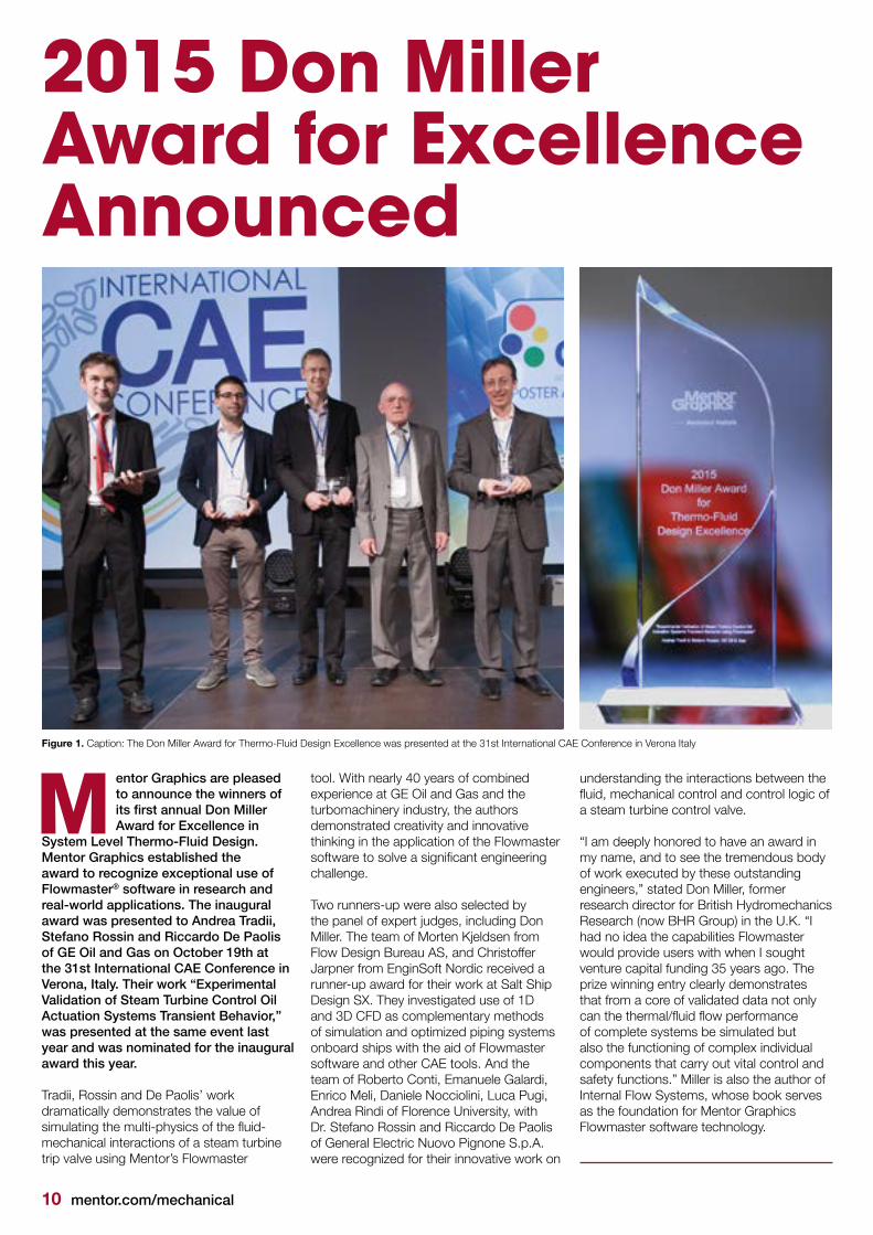
entor Graphics are pleased to announce the winners of its first annual Don Miller Award for Excellence in
System Level Thermo-Fluid Design. Mentor Graphics established the award to recognize exceptional use of Flowmaster® software in research and real-world applications. The inaugural award was presented to Andrea Tradii, Stefano Rossin and Riccardo De Paolis of GE Oil and Gas on October 19th at the 31st International CAE Conference in Verona, Italy. Their work “Experimental Validation of Steam Turbine Control Oil Actuation Systems Transient Behavior,” was presented at the same event last year and was nominated for the inaugural award this year.
Tradii, Rossin and De Paolis’ work dramatically demonstrates the value of simulating the multi-physics of the fluid-mechanical interactions of a steam turbine trip valve using Mentor’s Flowmaster
tool. With nearly 40 years of combined experience at GE Oil and Gas and the turbomachinery industry, the authors demonstrated creativity and innovative thinking in the application of the Flowmaster software to solve a significant engineering challenge.
Two runners-up were also selected by the panel of expert judges, including Don Miller. The team of Morten Kjeldsen from Flow Design Bureau AS, and Christoffer Jarpner from EnginSoft Nordic received a runner-up award for their work at Salt Ship Design SX. They investigated use of 1D and 3D CFD as complementary methods of simulation and optimized piping systems onboard ships with the aid of Flowmaster software and other CAE tools. And the team of Roberto Conti, Emanuele Galardi, Enrico Meli, Daniele Nocciolini, Luca Pugi, Andrea Rindi of Florence University, with Dr. Stefano Rossin and Riccardo De Paolis of General Electric Nuovo Pignone S.p.A. were recognized for their innovative work on
understanding the interactions between the fluid, mechanical control and control logic of a steam turbine control valve. “I am deeply honored to have an award in my name, and to see the tremendous body of work executed by these outstanding engineers,” stated Don Miller, former research director for British Hydromechanics Research (now BHR Group) in the U.K. “I had no idea the capabilities Flowmaster would provide users with when I sought venture capital funding 35 years ago. The prize winning entry clearly demonstrates that from a core of validated data not only can the thermal/fluid flow performance of complete systems be simulated but also the functioning of complex individual components that carry out vital control and safety functions.” Miller is also the author of Internal Flow Systems, whose book serves as the foundation for Mentor Graphics Flowmaster software technology.
MFigure 1. Caption: The Don Miller Award for Thermo-Fluid Design Excellence was presented at the 31st International CAE Conference in Verona Italy

mentor.com/mechanical 11
High Thermal Performance Copper - Graphene Heterostructures
istorically, porous materials have been of interest for a wide range of applications in thermal management,
for example, in heat exchangers and thermal barriers. Rapid progress in electronic and optoelectronic technology necessitates ever more efficient spreading and dissipation of the heat generated in these devices, calling for the development of new thermal management materials.
Effective thermal management is a crucial requirement for better performance and functionality of electronic and optoelectronic devices. The heat flux generated during operation is strongly linked to the device’s efficiency, lifetime, and failure. Effective removal of the heat generated is important, requiring heat transfer from the device to the ambient. Although only a small amount of power is required to operate a single LED, large heat fluxes exist in LED chips driven at high forward currents due to their small geometric size, operation at elevated ambient temperatures and Joule heating in both the contacts and the p-n junction. In microprocessors, overheating of the components results in performance degradation and failure of a system. For high-performance devices and future integration of multiple microprocessor functions, much more efficient dissipation of the generated heat fluxes will be needed.
Porous structures are very attractive for thermal management purposes both for heat transfer or insulation depending on the material, in a diverse range of applications. The large surface areas
H
of the pores offer the possibility for substantial increases in heat transfer to another medium, such as a gas or liquid. Therefore, the geometries and surfaces of the porous structures with opened or closed pores are important factors that determine their thermal properties. From a material perspective, nanostructured carbon materials, including nanodiamonds, nanotubes and graphene,
are promising candidates for thermal management because of their superior thermal conductivities.
Graphene, and graphene composites in particular, have advantages in process compatibility with electronic devices. The extraordinary thermal properties of graphene are unfortunately restricted by its high anisotropy, which results in
Figure 1. (a) Schematic of synthesis of the porous heterostructure using microparticles; (b, c) SEM images of copper micro particles and porous structure; (c, inset) typical structure, 0.5 x 1 x 2 cm
News
12 mentor.com/mechanical
a cross-plane thermal conductivity that is two orders smaller than the in-plane value. To overcome this limitation, 3D porous graphene or graphene-based heterostructures have been suggested as ideal materials for thermal transport as well as for electrodes in energy devices.
Researchers from Korea Institute of Science and Technology (KIST); Chonnam National University, Korea University of Science and Technology (UST); and the Korea Photonics Technology Institute combined forces to develop a strategy for the synthesis of a 3D microporous graphene-copper heterostructure using chemical vapor deposition (CVD) and sintering of copper microparticles. These porous structures with graphene networks offered better heat conduction and their large surface areas increased the dissipation of the heat outside the structure. Full details can be found in the original article in Nature [1].
Thermal properties of the porous structures The thermal diffusivity, κ, of each of the porous structures was measured using the laser-flash method as a function of specimen temperature over the range from 298 K to 1173 K. Typical thermal conductivities of the samples were found to be around 210 Wm-1K-1 for the temperature range of interest for electronics cooling, with the k values of the porous copper and porous graphene/
copper heterostructures calculated to be 209 Wm−1K−1 and 214 Wm−1K−1, respectively at room temperature. These are smaller than bulk or thin film copper (at 300–400 Wm−1K−1) due to the pores in the structures. The gas (or vacuum) with low thermal conductivity filling the void space reduces the effective heat-carrying cross-section area.
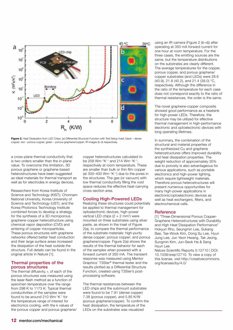
Cooling High-Powered LEDsRealizing these structures could potentially be applied to thermal management for optoelectronic devices, high-power vertical LED chips (2 × 2 mm2) were mounted on three substrates using silver paste, as shown in the inset of Figure 2(a), to compare the thermal performance of the substrate materials: high-purity dense copper; porous copper; and porous graphene/copper. Figure 2(a) shows the results of the thermal behavior for each of the samples when powered with a forward current of 350 mA. The transient response was measured using Mentor Graphics’ T3Ster® thermal tester and the results plotted as a Differential Structure Function, created using T3Ster’s post-processing software.
The thermal resistances between the LED chips and the submount substrates were found to be 7.91 (dense copper) 7.38 (porous copper), and 5.85 K/W (porous graphene/copper). To confirm the heat dissipation, the temperature of the LEDs on the substrates was visualized
using an IR camera (Figure 2 (b–d)) after operating at 350 mA forward current for one hour at room temperature. For the three cases, the emitting sources are the same, but the temperature distributions on the substrates are clearly different. The average temperatures for the copper, porous copper, and porous graphene/copper substrates (and LEDs) were 28.6 (40.9), 21.8 (40.2), and 21.4 (39.0) °C, respectively. Although the difference in the ratio of the temperature for each case does not correspond exactly to the ratio of thermal resistances, the order is the same.
The novel graphene-copper composite showed good performance as a heatsink for high-power LEDs. Therefore, the structure may be utilized for effective thermal management in high-performance electronic and optoelectronic devices with long operating lifetimes.
In summary, the combination of the structural and material properties of the synthesized Cu and graphene heterostructures offers improved durability and heat dissipation properties. The weight reduction of approximately 35% due to porosity is also advantageous for various applications, such as portable electronics and high-power lighting, which require lightweight materials. Therefore porous heterostructures will present numerous opportunities for many high-power applications in electronic/optoelectronic devices as well as heat exchangers, filters, and electrochemical cells.
Reference[1] “Three-Dimensional Porous Copper-Graphene Heterostructures with Durability and High Heat Dissipation Performance”Hokyun Rho, Seungmin Lee, Sukang Bae, Tae-Wook Kim, Dong Su Lee, Hyun Jung Lee, Jun Yeon Hwang, Tak Jeong, Sungmin Kim, Jun-Seok Ha & Sang Hyun Lee Nature Scientific Reports 5:12710 | DOI: 10.1038/srep12710. To view a copy of this license, visit http://creativecommons.org/licenses/by/4.0/
Figure 2. Heat Dissipation from LED Chips; (a) Differential Structure Function with Test Setup Inset; black – dense copper; red – porous copper; green – porous graphene/copper; IR images (b-d) respectively.

mentor.com/mechanical 13
he goal of electronics thermal design is to accurately predict component junction temperatures to ensure that
they are within specification. Easier said than done. Before CFD was used, designers used simple metrics, such as junction-to-case thermal resistance, as a ‘thermal model’ of the component in calculations by hand, with very wide safety margins to ensure the design was thermally viable. CFD allowed designers to predict the flow of cooling air, and include 3D thermal simulations of the board and components, increasing the need for more accurate component-level modeling.
Various methods were devised in the 1990s. Junction-to-case and junction-to-board thermal metrics were combined to form a 2-resistor model, and the DELPHI Consortium developed multi-resistor models that accounted for multiple heat flow paths in the package, increasing the predictive accuracy further. The most accurate thermal models, which also account for transient effects and are able to handle multi-die packages, are detailed 3D conduction models. The increasing use of miniaturized high-powered devices and High Density Interconnection boards intensifies the coupling effect with neighboring thermally-sensitive components, increasing the need to predict the temperatures of all components accurately.
The Thales Corporate Engineering Thermal Team is responsible for the introduction of new technologies inside the Thales Group and is consequently
T
Electronics Thermal Design with Thales and FloTHERM® XT
at the leading edge of thermal research. This is aimed at achieving more accurate simulation results in the shortest possible time to meet the industrial requirements of the divisions they support, including Defense, Aerospace & Space and Security. As a DELPHI consortium partner, the team has continued its own research on the use of reduced order models, created from detailed models, to provide Thales’ divisions with the resources they need through Thales’ Thermal Analysis Workbench (WATT).
Until now, this effort has been hampered by the inability to incorporate all thermally-relevant details into the detailed model due to the large number of microscopic elements that are present within an electronic component. More than ever, a fine representation of all the details of a small package is today mandatory to avoid an overestimation of the semiconductor temperature.
A Step Further in Thermal Modeling of Electronic ComponentsBy Eric Monier-Vinard, Thermal Domain Manager, Thales Corporate Engineering
Figure 1. Thales’ Thermal Analysis Workbench (WATT)
Figure 2. The realistic modeling of a QFN 16 package reduces the temperature prediction by 20%
Aerospace

14 mentor.com/mechanical
There has always been a conservative design margin applied at the component level due to the fact that it has either taken too long or simply been impractical to take into account all the geometries inside a component package. For example, the detailed copper traces, copper vias on the substrate as well as the bond wires between the die and the substrate were rarely modeled explicitly, but are known to contribute to the heat spreading. Until now these very small elements were
either roughly represented by single parts with averaged thermal properties or simply ignored. Their replacement by single aggregated parts introduces some inaccuracies in the results, while ignoring them leads to a higher calculated temperature and consequently higher margins during the design process.
With FloTHERM™ XT, the Core Thermal Team has been able to take a major step forward, producing, in just a few hours,
results for System-in-Package devices or conventional BGA or LGA packages including all geometric elements inside the package.
For instance, the Thales Core Thermal Team has been able to import the complete geometry of a FpBGA 208 package with all its internal details as well as its supported board test vehicle, then set the general boundary conditions in just a few hours.
The meshing strategy of FloTHERM XT, which is based on the local size of the different parts of the model, requires very few user inputs and allows for the creation of an appropriate and easily solvable 1.9-million-cell mesh in less than three hours of computation on a 12-core Intel Xeon processor. The powerful solver needed less than 4.5 hours to reach full convergence on the same processor using 10 Gb of memory. This short computational time has allowed quick comparisons on the influence of the 25µm (1mil) bond wires on the package’s thermal performance both in natural convection and in forced convection at different velocities.
The numerical results are very close to the measurements already conducted on this component, and are within 1% for the natural convection case, as shown in Table 1.
Increased simulation accuracy is the only way to break the conservative design margins used in the past.
Respecting these former margins would cost a lot more today than in the past due to the increased power density, so it is essential that cooling systems are
Figure 3. Component on JEDEC 2s2p test board in FloTHERM XT, showing internal detail including bond wires
Table 1. Thermal performance comparison
Figure 4. Detail of heat spreading throughout complex copper traces and vias (inset: X-ray showing bond wires)
Velocity Model TEXP TCFD %E θjaEXP θjaCFD
V = 1 m/s Model without bond wires 146.2°C 149.4°C 2.1% 39.1°C/W 40.2°C/W
V = 1 m/s Model with bond wires 146.2°C 146.9°C <1% 39.1°C/W 39.3°C/W
V = 2 m/s Model without bond wires 93.0°C 95.0°C 2.8% 23.9°C/W 24.6°C/W
V = 2 m/s Model with bond wires 93.0°C 92.6°C 0.6% 23.9°C/W 23.8°C/W

mentor.com/mechanical 15
made as efficient as possible, and for that simulation accuracy at all packaging levels is needed.
Further, a fine representation of FpBGA 208 internal structure permits to better understand the thermal constraints encountered by the PCB interconnect balls, especially at corner locations. Figure 3 highlights a temperature gradient of 48°C for the set of interconnect balls.
If the modeling of the internal structure of the electronic component is crucial to
Figure 5. FloTHERM XT is poised to take a major role in Thales’ overall Thermal Design Workflow
“The thermal design of electronic component is under increasing control. With FloTHERM XT we can import the complete geometry of a FpBGA 208 package with all its internal details, test board, setup the boundary conditions and solve it in just a few hours. This will allow Thales to better integrate cooling systems, and comprehend previously misunderstood multiphysics issues.”Eric Monier-Vinard, Thermal Domain Manager, Thales Corporate Engineering
accurately predict the temperature of its chip(s), the layer layout and copper trace design of the electronic board is now essential to efficiently optimize the way the heat is spread throughout its structure. Even there FloTHERM XT can simulate the small and thin elements that make up its composite structure.
This new approach, afforded by FloTHERM XT, means that the conservative design margins of the past can be reviewed, paving the way to accurately predict the thermal behavior
of systems at all packaging levels, and particularly at the component level where the highest temperature gradients are located. This will allow Thales to better integrate cooling systems, even in cases where it was impossible with the old conservative margins. And sometimes it helps to comprehend previously misunderstood multiphysics issues.
Aerospace

Automotive
Lighting the Way
he style of a car is very much characterized by its lighting system. The final product is created by the collaboration
between three areas of competence: Design, Thermal Management and Photometry in the pre-development phase. To show their expertize, Bertrandt engineers developed their own full-LED headlamp and exhibited it at the IAA 2013 in Frankfurt, Germany. The thermal analysis of the IAA exhibit was carried out using the thermal simulation software FloEFD™ from Mentor Graphics. General ConsiderationsThe creation of light inherently generates heat [1] [2]. The most common light sources nowadays are incandescent lamps and LEDs. Incandescent lamps are thermal radiators (black bodies) which emit a tiny fraction of energy in the visible spectrum. LEDs are semiconductors which release photons through the recombination process. Just as there are differences in the light creation processes, there are also different demands regarding the thermal management of the light sources. Incandescent bulbs need a minimum temperature for the filament to produce light. LEDs are "cold" emitters and require efficient cooling of the optically active junction layer to meet the requirements of service life and the emission spectrum. Compared to halogen bulbs, light-emitting diodes have a higher optical efficiency, lower heat generation and a longer service life. In addition, they provide designers with more creative freedom due to their smaller dimensions, directed light emission and greater freedom within the constraints of lighting legislation [3]. Given these advantages, the tendency towards using LEDs in the automotive industry is steadily growing. As a consequence, the demands on the LED lights are also higher. They are expected to offer higher performance
T
By Kibriye Sercan, Michael Hage, Mario Dotzek and Eugen Tatartschuk, Bertrandt Group, Cologne , Germany
Development of the Bertrandt Full-LEDHeadlight Thermal Simulation and Design
mentor.com/mechanical 17
18 mentor.com/mechanical
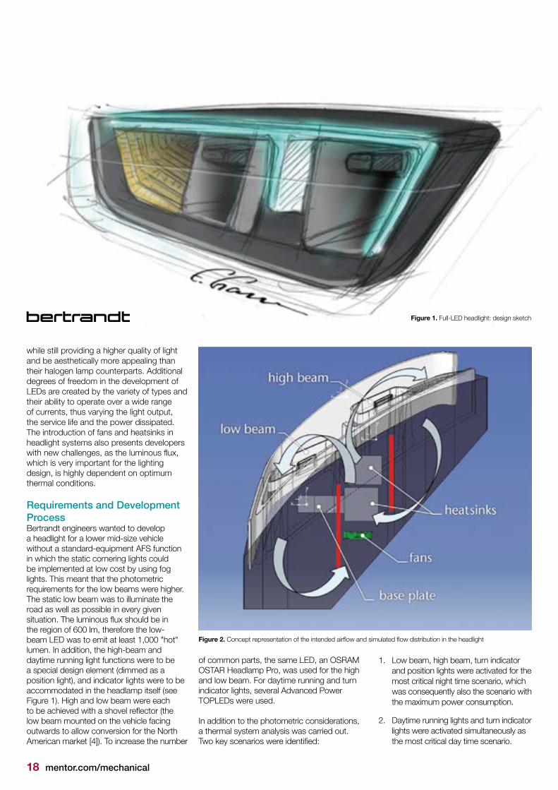
Figure 2. Concept representation of the intended airflow and simulated flow distribution in the headlight
while still providing a higher quality of light and be aesthetically more appealing than their halogen lamp counterparts. Additional degrees of freedom in the development of LEDs are created by the variety of types and their ability to operate over a wide range of currents, thus varying the light output, the service life and the power dissipated. The introduction of fans and heatsinks in headlight systems also presents developers with new challenges, as the luminous flux, which is very important for the lighting design, is highly dependent on optimum thermal conditions.
Requirements and Development ProcessBertrandt engineers wanted to develop a headlight for a lower mid-size vehicle without a standard-equipment AFS function in which the static cornering lights could be implemented at low cost by using fog lights. This meant that the photometric requirements for the low beams were higher. The static low beam was to illuminate the road as well as possible in every given situation. The luminous flux should be in the region of 600 lm, therefore the low-beam LED was to emit at least 1,000 "hot" lumen. In addition, the high-beam and daytime running light functions were to be a special design element (dimmed as a position light), and indicator lights were to be accommodated in the headlamp itself (see Figure 1). High and low beam were each to be achieved with a shovel reflector (the low beam mounted on the vehicle facing outwards to allow conversion for the North American market [4]). To increase the number
of common parts, the same LED, an OSRAM OSTAR Headlamp Pro, was used for the high and low beam. For daytime running and turn indicator lights, several Advanced Power TOPLEDs were used.
In addition to the photometric considerations, a thermal system analysis was carried out. Two key scenarios were identified:
1. Low beam, high beam, turn indicator and position lights were activated for the most critical night time scenario, which was consequently also the scenario with the maximum power consumption.
2. Daytime running lights and turn indicator lights were activated simultaneously as the most critical day time scenario.
Figure 1. Full-LED headlight: design sketch

mentor.com/mechanical 19
Figure 3. First airflow simulation without a cover frame. The circulations develop as planned. Part of the warm air slips through the cooling channel at the position where the base plate of the LED leaves a gap
Figure 4. Thermal simulation with fully designed heatsinks and cover frame. Through several iterations and changes of the airflow guide, it was possible to design the airflow to be similar to the original plan. The base plates of the LEDs are wide enough to conduct the necessary amount of heat.
In these two scenarios as a continuous condition, the junction temperatures of the LEDs should not exceed the maximum permissible values. A further aim was to direct the warm air from the main lighting functions (low and high beam) to the front of the cover frame, both to defog the lens and to cool the air in the lamp.
The development was carried out in the following steps:
3. Concept phase:
• LED pre-selection
• Heatsink positioning
• Number of fans and possible positions
4. Dimensioning/layout:
• Heatsink size and shape
• Size of base plates
5. Adaptation of LED type
6. Design of the heatsink ribs and adaptation:
• Size
• Shape
• Airflow direction
7. Air routing and cover frame8. Fan selection
Through this process, which was partly iterative and partly connected with other disciplines such as lighting design, the developers succeeded in achieving the photometric objectives and the design of an efficient cooling system to attain the desired LED lifetime.
Cooling ConceptTo meet the photometric requirements of the low beam, a powerful four-chip LED was chosen during the design phase. Based on the thermal resistance of the LED and estimates for the heatsinks, checks were run on whether the required luminous flux under the junction temperature of T = 150°C could be achieved. A particular challenge for cooling the low-beam LED is its position at the top of the headlight. With these design specifications, the low beam is deemed thermally more critical than the other functions. As a result of limited space in the upper housing portion, the LED was not placed directly on the heatsink, but had to be connected to the heatsink via a base
plate. This resulted in additional thermal resistance, which was confirmed both by simulations and by analytical assessments. The decision was then made to move to the five-chip LED LE UW U1A5 01, which has a thermal resistance of 1.5K/W [5], because it could be operated with a lower current and achieve the same luminous flux. Since the natural convection was hampered by the heatsink shape and position, a fan was
Automotive
20 mentor.com/mechanical
utilized. This allowed good circulation of the air in the headlight, and a reduction in the size of the heatsinks (Figure 2).
The heatsink of the high beam was placed in front of the low beam heatsink, between the reflectors for the main lighting functions. Directly behind it, there is a fan that blows air through the two heatsinks in the vehicle's direction of travel. As a result, an air channel is created between the reflectors (Figure 3) which contributes to efficient cooling and air circulation. With the aid of Mentor Graphics’ FloEFD™ 3D simulation software, the flow distribution was determined and the bezel geometry defined accordingly. The warm air was blown out of the heatsinks through an opening in the bezel below the centre section of the daytime running lights and against the cold lens, where the air cools down and simultaneously defogs the front lens. In two cycles, the cold air flows back behind the bezel and into the fan. The resulting cooling circuits are shown in Figure 2 (red lines indicate the air guide). It should be noted that two circuits are easier to control than one circulating around the entire headlight.
Using a parametric model of the heatsink and the FloEFD parametric study feature with post-processing [6], the heatsink fins were designed for the main lighting functions in order to ensure the most efficient cooling for a given airflow. The model was then completed for the signal light LED functions as well as
their heatsinks. Based on the aerodynamic resistance of the system, an axial fan was chosen to work in conjunction with this system at its optimum operating point.
ResultsOnce the system was fully represented as a CAD model with the housing, lens, cover, air duct, fan, and heatsink, it was possible to run a simulation with precise LED parameters, a characteristic fan curve and boundary conditions in the two aforementioned scenarios. From these simulations, the operating current was calculated, which allowed an LED to operate below the critical temperature in typical conditions. All lighting functions were achieved at an ambient temperature of around 50°C at the lens and at 90°C on the housing in accordance with ECE regulations and performance requirements. This was also demonstrated with in-house measurements in continuous operation of the headlight [7].
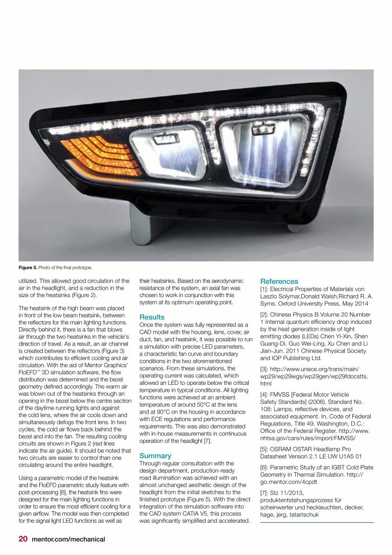
SummaryThrough regular consultation with the design department, production-ready road illumination was achieved with an almost unchanged aesthetic design of the headlight from the initial sketches to the finished prototype (Figure 5). With the direct integration of the simulation software into the CAD system CATIA V5, this process was significantly simplified and accelerated.
References[1]: Electrical Properties of Materials von Laszlo Solymar,Donald Walsh,Richard R. A. Syms. Oxford University Press, May 2014
[2]: Chinese Physics B Volume 20 Number 1 Internal quantum efficiency drop induced by the heat generation inside of light emitting diodes (LEDs) Chen Yi-Xin, Shen Guang-Di, Guo Wei-Ling, Xu Chen and Li Jian-Jun. 2011 Chinese Physical Society and IOP Publishing Ltd.
[3]: http://www.unece.org/trans/main/wp29/wp29wgs/wp29gen/wp29fdocstts.html
[4]: FMVSS [Federal Motor Vehicle Safety Standards] (2006). Standard No. 108: Lamps, reflective devices, and associated equipment. In, Code of Federal Regulations, Title 49. Washington, D.C.: Office of the Federal Register. http://www.nhtsa.gov/cars/rules/import/FMVSS/
[5]: OSRAM OSTAR Headlamp Pro Datasheet Version 2.1 LE UW U1A5 01
[6]: Parametric Study of an IGBT Cold Plate Geometry in Thermal Simulation. http://go.mentor.com/4cpdt
[7]: Stz 11/2013, produktentstehungsprozess für scheinwerfer und heckleuchten, decker, hage, jerg, tatartschuk
Figure 5. Photo of the final prototype.

mentor.com/mechanical 21
Experimental Validation of Steam Turbine Control Oil Actuation Systems Transient Behavior[1]
his work presented at the 30th International CAE Conference in Verona, Italy demonstrates dramatically the value of
simulating the multi-physics of the fluid-mechanical interactions of a steam turbine trip valve. The steam trip valves are used as a safety device to prevent a steam turbine from overspinning. Also called overspeed valves, they shut down the flow of steam to the turbine on overspeed if it reaches 10% above the maximum operational speed. These valves use a high spring force, opposed by control oil pressure during normal operation, to close the hydraulically controlled valve rapidly on loss of control oil pressure. This creates a close coupling between the steam flow path and the hydraulic control fluid path via the mechanical interaction of the valve. The authors were able to successfully model this interaction by taking advantage of the Flowmaster mechanical component library. The model had to properly demonstrate the three stages of operation which include:
• Opening stage: loading of the spring;
• Opening stage: valve opening; and
• Closing stage. The model was validated against test data and the team were able to successfully simulate the pressure fluctuations behind the damper plate of the valve and show the decoupling between the damper plate and the piston glass at the end of the opening phase of the valve trip.
Once the valve control was validated it was able to convert to a composite component and then added to a master model that simulated an entire test bench oil systemThis complete piping model was based on
the real components and was validated through a series of tests which showed good correlation. By running through a number of scenarios by the team were able to optimize the control oil system by adjusting several parameters including pipe diameters, orifice sizes, pipe lengths, and external temperature.
From their physical tests and numerous simulations runs the authors were able to successfully model both the hydrodynamic
and mechanical interactions simultaneously in Flowmaster. This provided them with fast consistent simulations in different configurations and run virtual hazardous operational scenarios. It also gives them the opportunity to provide fast solutions for customer problems and eliminates the need for tuning of the system during installation.
Riccardo De Paolis graduated in Mechanical Engineering from University “RomaTre” in fall 2013, carrying out turbomachinery and electric machines path. For his first work experience, he joined a
TAndrea Tradii; Stefano Rossin; and Riccardo De Paolis, GE Oil and Gas
2015 Don Miller Award for Excellence in System Level Thermo-Fluid Design
Figure 1. Steam path components
Process

22 mentor.com/mechanical
six month internship with GE Oil & Gas, increasing software modeling of various Gas Turbines Auxiliary Systems. At the end of the internship, he succeeded in GE Oil & Gas Edison Engineering Development Program selection, being part of this leadership program from wave 2014. The first rotational assignment he carried out was still related to Gas Turbine Auxiliary Systems, giving contribution in one-dimensional fluid dynamics and Finite Elements Modeling, as well as completing requisition activities.
Stefano Rossin currently holds the position of Chief Engineer for Turbomachinery Auxiliary System and Industrial Plant in GE Oil&Gas based in Florence. He graduated from the University of Pisa with a M.S. Degree in Aeronautical Engineering and he began his career in 1989 working in several fields from Chemical Research to Aerospace.
He joined GE O&G in 2005 and since then he has always managed the design of rotating machineries auxiliary systems, improving connections with universities in several engineering areas and successfully introducing fundamental guidelines for blast assessment of turbo-compressor train, in off-shore and Floating Liquefied Natural Gas applications.
He is the author of three patents and 15 international papers, some of them developed in cooperation with important Oil&Gas customers such as Shell and Exxon Mobil. In June 2013 Stefano received the Edison Pioneer Award, such honor is presented to select individuals from across GE every year and it recognizes mid-career technologists who demonstrate technical excellence and customer impact.
Andrea Tradii is Senior Engineer for Turbomachinery Auxiliary System and Industrial Plant in GE Oil&Gas based in Florence. He graduated at the University of Rome and joined GE O&G in 1991. Since then he managed the design of Mechanical Auxiliary Systems for Turbo-compressor trains and Motor-compressor trains. He began his career as a Mechanical Design Engineer and, after four years of experience as Resident Engineer in Mexico, he became Mechanical Team Leader for Turbomachinery Auxiliary System. In 2012 he was appointed Product Innovation and Standard Update Leader.
Reference: [1] Presented as part of the International CAE Conference proceedings, Oct. 2014
Figure 2. Mechanical components of hydraulic actuator
Figure 3. Hydraulic model characterization
Figure 4. Control oil actuation systems validation

mentor.com/mechanical 23
System Control logic enhancements through Fluid-Mechanical valve dynamic transfer functions[1]
heir paper describes the innovative work completed by the authors to better understand the interactions between the fluid, mechanical
control, and control logic of a steam turbine control valve. In situations such as this, mechanical limitations, manufacturing tolerances, and approximation errors in the control logic can cause a system to react in unexpected ways and that then needs to be fine-tuned to operate properly. In a worst case scenario, error propagation in transient situations can cause system response drift which cannot be recovered from. This can produce unknown and possibly damaging consequences. The authors attempted to reproduce such a scenario through simulation in order to understand the root causes of the response drift, and to then develop control logic that could prevent the loss of control.
A steam turbine control valve is used to control and manage the amount of steam allowed to enter the steam turbine and thereby produce a consistent power output. For this system, pressurized oil is used to actuate the heavy control valves. The oil needs to be metered precisely in order for the system to maintain the desired power output. This control is managed by a Control Pressure Converter (CPC) which operates in a similar way to a PID controller. The control valve also consists of a series of levers and a spring to manage the position of the valve.
All of these components and their interactions with the fluid system must be taken into consideration when simulating the system. The authors did this by constructing a fluid mechanical multi-physics model in Flowmaster utilizing the mechanical component library. The library includes springs, levers, cylinders
and control ports that can be linked together to construct a control valve from its individual components. The control logic was added to the model via the Flowmaster controller template and scripting. The Flowmaster model was run in a transient simulation and the obtained results were compared against controlled experimental test data. It can be seen that the simulation results showed good correlation with the experimental data. The goal was to create a transfer function that could be used in a Simulink® model, so the control logic could be fine-tuned to prevent the loss of control. The intrinsic transient behavior of this particular system made it
impossible. To bypass this limitation, a Simulink model of the control valve was created and the Flowmaster results were used to validate that Simulink model. From there the control logic could then be modified to achieve the desired valve operation. Future work will be to integrate the Flowmaster and the Simulink models so changes made in the control logic model can be seen immediately in the multi-physics model in Flowmaster.
Reference:[1] First published in Newsletter EnginSoft Year 11 No. 2
TBy R. Conti, E. Galardi, E. Meli, D. Nocciolini, L. Pugi, A. Rindi of Florence University and Dr. S. Rossin, R. De Paolis General Electric Nuovo Pignone S. p. A.
2015 Don Miller Award Runner Up
Figure 1. Steam control valve and main components
Figure 2. Steam control valve Flowmaster network Figure 3. Figure 8, control system computational model vs. experimental behavior
Power Generation
24 mentor.com/mechanical
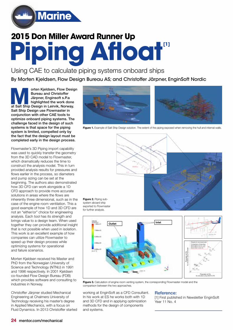
orten Kjeldsen, Flow Design Bureau and Christoffer Järpner, Enginsoft s.P.a highlighted the work done
at Salt Ship Design in Leirvik, Norway. Salt Ship Design use Flowmaster in conjunction with other CAE tools to optimize onboard piping systems. The challenge faced in the design of such systems is that space for the piping system is limited, compelled only by the fact that the design layout must be completed early in the design process.
Flowmaster’s 3D Piping import capability was used to quickly transfer the geometry from the 3D CAD model to Flowmaster, which dramatically reduces the time to construct the analysis model. This in turn provided analysis results for pressures and flows earlier in the process, so diameters and pump sizing can be set at the beginning. The authors also demonstrated how 3D CFD can work alongside a 1D CFD approach to provide more accurate solutions in areas where the flows are inherently three dimensional, such as in the case of the engine room ventilation. This a good example of how 1D and 3D CFD are not an “either/or” choice for engineering analysis. Each tool has its strength and brings value to a design team. When used together they can provide additional insight that is not possible when used in isolation. This work is an excellent example of how companies can utilize Flowmaster to speed up their design process while optimizing systems for operational and failure scenarios. Morten Kjeldsen received his Master and PhD from the Norwegian University of Science and Technology (NTNU) in 1991 and 1996 respectively. In 2001 Kjeldsen co-founded Flow Design Bureau (FDB) which provides software and consulting to industries in Norway.
Christoffer Järpner studied Mechanical Engineering at Chalmers University of Technology receiving his master’s degree in Applied Mechanics, with a focus on Fluid Dynamics. In 2013 Christoffer started
Piping Afloat[1]
M
2015 Don Miller Award Runner Up
Using CAE to calculate piping systems onboard ships
Results for non-tuned exitsComparison of branches:Branch A(Exit 5,12 & 15): -2.9%Branch B(Exit 6,10 & 14): 9.6%Branch C(Exit 7,8 & 9): 0%
InletOutlet Branch B(Exit 10, 14 & 6)
Branch C(Exit 7, 8 & 9)
Branch A(Exit 12, 15 & 5)
By Morten Kjeldsen, Flow Design Bureau AS; and Christoffer Järpner, EnginSoft Nordic
Marine
Figure 2. Piping sub-system aboard ship exported to Flowmaster for further analysis.
Figure 3. Calculation of engine room venting system, the corresponding Flowmaster model and thecomparison between the two approaches.
Figure 1. Example of Salt Ship Design solution. The extent of the piping exposed when removing the hull and internal walls.
working at EnginSoft as a CFD Consultant. In his work at ES he works both with 1D and 3D CFD and in applying optimization methods for the design of components and systems.
Reference:[1] First published in Newsletter EnginSoft Year 11 No. 4

mentor.com/mechanical 25
btaining an accurate prediction of junction and case temperature for IC packages has always been
an important part of thermal simulations of electronics. In the past decade or so the industry has seen important improvements in terms of creating Compact Thermal Models (CTMs) for components. FloTHERM® PACK uses the standards defined and published by JEDEC to create both 2-R and Delphi compact models.
Fortunately, more and more manufacturers of IC packages are creating Delphi models of their packages. This makes it possible for the end users to predict the junction and case temperature of the package in the system level simulation and to obtain boundary condition independent results. Knowing the fact that package manufacturers (with very few exceptions) are very reluctant to reveal the information about the internal structure of their packages, makes these Delphi models very desirable and valuable for end users.
In considering 2-R and Delphi models for components, it is important to mention that 2-R CTMs are defined and meant to be comparative metrics rather than predicting junction and case temperature for a package at different environmental conditions. Delphi models are preferred CTMs and have clear advantages over 2-R models as they provide boundary condition independent results.
For a detailed discussion on different CTMs for IC packages, their differences, pros and
O
Transient Thermal Simulations and Compact Components: A Review
Ask The GSS Expert
cons, please refer to Robin Bornoff's blog series:
http://go.mentor.com/RobinBornoffBlog
It is the common experience that a 2-R model will have an error in the range of 20%-30% (depending on the package style and environment conditions). A Delphi model, on the other hand, has under 10% error. The computational expense of a Delphi model over 2-R model is very small so, we recommend using Delphi models when available.
It goes without saying that a detailed model of an IC package, when available, will be the most accurate one. FloTHERM PACK will create detailed models of many package families (apart from 2-R and Delphi compact models). It is recommended to use a detailed model for packages that are thermally critical. The drawback is that it is computationally more expensive to model the packages in detail.
The above is a quick summary of available options when it comes to modeling IC packages in steady state situations.
In thermal simulation of electronics however, there are many situations where we are interested in transient behavior of IC packages. To this end, similar to steady state situations, a detailed model of an IC package is the obvious answer. When the package is modeled in detail, with geometry and material defined for all objects inside the package, the CFD simulation will provide the temperature (of the die for example) as a function of time.
The key here is to make sure that specific heat and density are correctly defined for all materials in the package. These material properties become irrelevant in steady state simulations as they appear with time-dependent terms in the equations. So, it is important to make sure these values are correct in transient simulations for different parts inside the package (and for the materials in the rest of the system). Specific heat has the dimensions of J/kg K and in essence is a measure of how quickly or how slowly a material heats up when subjected to a certain amount of heat.
How about using CTMs in transient situations? The answer is that 2-R and Delphi models are not capable of predicting transient behavior of the package. They are basically resistor networks. 2-R is a two resistor network and Delphi model is a boundary condition independent multi-resistor network (in a Delphi CTM, depending on the package style, there will be a different number of resistors defining the package). In order to predict the transient junction temperature for instance, the CTM should include the capacitance as well.
At present time, JEDEC definition of 2-R and Delphi compact models determines thermal resistance values in steady state and does not include thermal capacitances. Therefore FloTHERM PACK does not create such capacitance values.
FloTHERM PACK however, offers the option to create the Delphi compact model in the form of a Network Assembly. Network Assembly is essentially the same
What are some methods for thermal modeling of an IC package in steady state and transient conditions?By Akbar Sahrapour, Senior Thermal Consultant Engineer, Mentor Graphics
26 mentor.com/mechanical
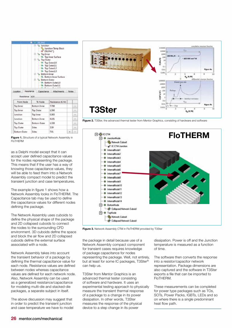
Figure 1. Structure of a typical Network Assembly in FloTHERM
the package in detail because use of a Network Assembly compact component for transient cases requires knowledge of package capacitance for nodes representing the package. Well, not entirely, but at least for some IC packages, T3Ster® can help us.
T3Ster from Mentor Graphics is an advanced thermal tester consisting of software and hardware. It uses an experimental testing approach to physically measure the transient thermal response of a package to a change in its power dissipation. In other words, T3Ster measures the response of the physical device to a step change in its power
dissipation. Power is off and the Junction temperature is measured as a function of time.
The software then converts the response into a resistor/capacitor network representation. Package dimensions are also captured and the software in T3Ster exports a file that can be imported to FloTHERM.
These measurements can be completed for power type packages such as TOs, SOTs, Power Packs, IGBTs, LEDs and so on where there is a single predominant heat flow path.
FloTHERM
T3Ster
as a Delphi model except that it can accept user defined capacitance values for the nodes representing the package. This means that if the user has a way of knowing those capacitance values, they will be able to feed them into a Network Assembly compact model to predict the transient junction and case temperatures.
The example in figure 1 shows how a Network Assembly looks in FloTHERM. The Capacitance tab may be used to define the capacitance values for different nodes defining the package.
The Network Assembly uses cuboids to define the physical shape of the package and 2D collapsed cuboids to connect the nodes to the surrounding CFD environment. 3D cuboids define the space and block the air flow and 2D collapsed cuboids define the external surface associated with a node.
Network Assembly takes into account the transient behavior of a package by defining the thermal capacitance value for each node. Resistance values are defined between nodes whereas capacitance values are defined for each network node.Also, Network Assembly can be used as a generalized resistance/capacitance for modeling multi-die and stacked-die packages, a separate subject in itself.
The above discussion may suggest that in order to predict the transient junction and case temperature we have to model
Figure 2. T3Ster, the advanced thermal tester from Mentor Graphics, consisting of hardware and software
Figure 3. Network Assembly CTM in FloTHERM provided by T3Ster

mentor.com/mechanical 27
ith LED lighting technologies, the mechanical design of the luminaire is the most
important aspect in meeting industry demands for cost and performance.
The shape of the body, type, and number of the fins on the external casing, and the selection of the casing and other materials are the main mechanical parameters affecting the cooling of the luminaire. All these parameters also affect the weight and cost of the luminaire, so mechanical optimization is critical to optimizing the product cost.
All LED manufacturers try to design smaller and more thermally effective luminaires through the use of CFD. For Vestel’s Ephesus street light luminaire, FloEFD™ was used to optimize both the thermal design and to check the drag force on the luminaire when pole mounted, to ensure compliance with national standards for wind loading.
LEDs are unique amongst light sources in that they are designed to operate at low temperatures through the efficient conduction of heat away from the LED. LEDs generate little or no IR or UV, but convert only 15%-25% of the power into visible light; the remainder is converted to heat that must be conducted from the LED die to the underlying circuit board and heatsinks, housings, or luminaire frame elements in order to limit the junction temperature during operation, otherwise the light output falls [1]. In addition to reduced lumen output, excess heat directly shortens LED lifetime, and the lifetime of any control circuitry within the luminaire.
The challenge facing lighting companies is to design a luminaire that has the maximum thermal performance while minimizing the costs related to the materials used and
LED Lighting
Cost Optimization of LED Street LightingLED Lighting Technologies from Vestel EngineeringBy Emre Serdar & İsmail Güngör, Sr. Mechanical Design Engineers, Vestel Electronic – LED Lighting
W
the mechanical design. As these are the largest overall contribution to the cost of the luminaire, there is a strong drive to minimize the mechanical cost through optimization of the thermal design.
The design goals for a luminaire should be based either on an existing fixture’s performance or on the application’s lighting requirements. So, the design steps start with researching existing product designs as benchmarks, used to develop a target
Figure 1. Relative Luminous Flux vs. Junction Temperature of White Cree XT-E (350 mA forward current)
Figure 2. Design Steps
28 mentor.com/mechanical
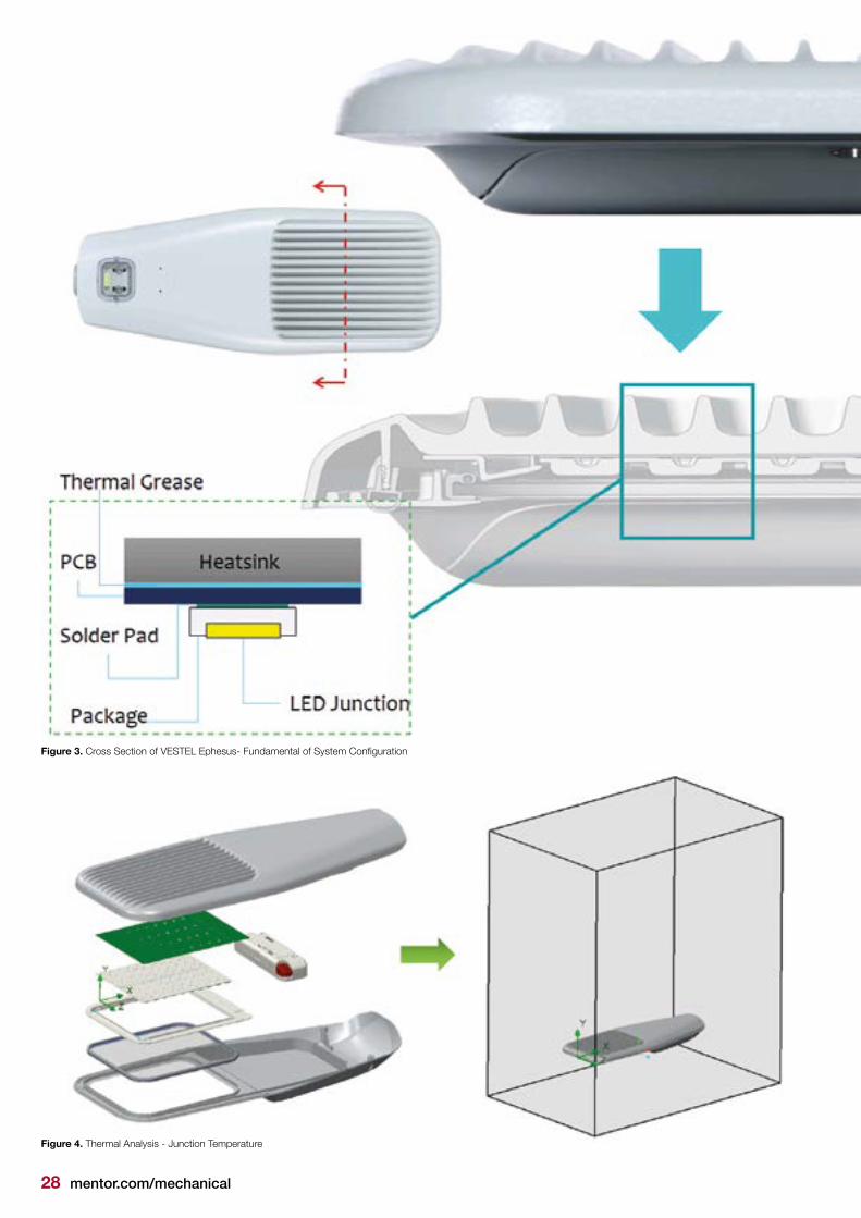
Figure 3. Cross Section of VESTEL Ephesus- Fundamental of System Configuration
Figure 4. Thermal Analysis - Junction Temperature
mentor.com/mechanical 29
specification for the product. The designer should specify any other goals that will influence the design, such as special optical and hardware requirements, like the selection of LED chips, drive current, etc. directly impacts thermal performance, and hence the mechanical design.
After the defining goals, in accordance with the optical and hardware requirements, choosing the type and number of LEDs and the drive current for the LED chips, the designer should start the mechanical design. Once an acceptable mechanical design is achieved this can be used for a first thermal analysis, and subsequent optimization study.
System ConfigurationTo design an effective cooling solution as part of the luminaire design, designers and analysts need to fully understand those aspects of the design that affect thermal performance, and the principle of thermal resistance. Three things affect the junction temperature of an LED chip: drive current, thermal path, and ambient temperature. In general, the higher the drive current, the greater the heat generated at the die. Heat must be moved away from the die in order to maintain expected light output, color, and lifetime
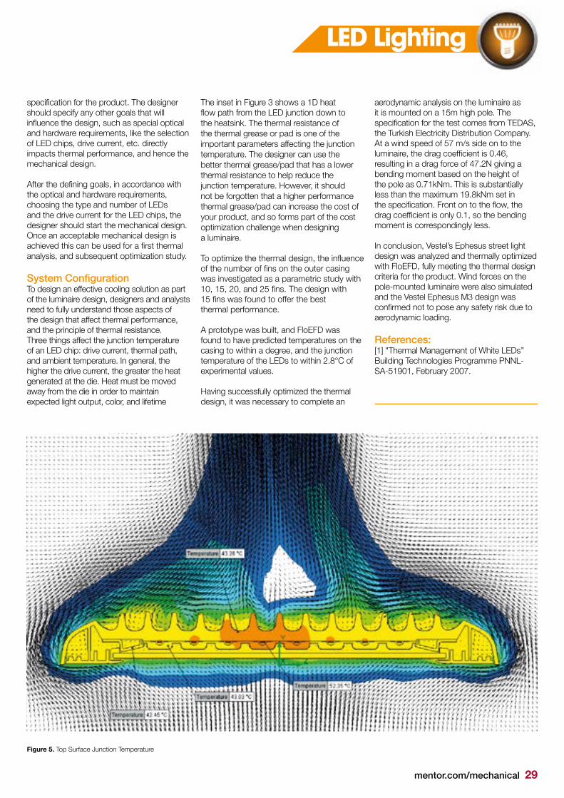
The inset in Figure 3 shows a 1D heat flow path from the LED junction down to the heatsink. The thermal resistance of the thermal grease or pad is one of the important parameters affecting the junction temperature. The designer can use the better thermal grease/pad that has a lower thermal resistance to help reduce the junction temperature. However, it should not be forgotten that a higher performance thermal grease/pad can increase the cost of your product, and so forms part of the cost optimization challenge when designing a luminaire.
To optimize the thermal design, the influence of the number of fins on the outer casing was investigated as a parametric study with 10, 15, 20, and 25 fins. The design with 15 fins was found to offer the best thermal performance.
A prototype was built, and FloEFD was found to have predicted temperatures on the casing to within a degree, and the junction temperature of the LEDs to within 2.8°C of experimental values.
Having successfully optimized the thermal design, it was necessary to complete an
aerodynamic analysis on the luminaire as it is mounted on a 15m high pole. The specification for the test comes from TEDAS, the Turkish Electricity Distribution Company. At a wind speed of 57 m/s side on to the luminaire, the drag coefficient is 0.46, resulting in a drag force of 47.2N giving a bending moment based on the height of the pole as 0.71kNm. This is substantially less than the maximum 19.8kNm set in the specification. Front on to the flow, the drag coefficient is only 0.1, so the bending moment is correspondingly less.
In conclusion, Vestel’s Ephesus street light design was analyzed and thermally optimized with FloEFD, fully meeting the thermal design criteria for the product. Wind forces on the pole-mounted luminaire were also simulated and the Vestel Ephesus M3 design was confirmed not to pose any safety risk due to aerodynamic loading.
References:[1] "Thermal Management of White LEDs’’ Building Technologies Programme PNNL-SA-51901, February 2007.
Figure 5. Top Surface Junction Temperature
LED Lighting

Tablet TeardownBy Arun Raghupathy & Bharath NagendranElectronic Cooling Solutions Inc.
Challenges in the Thermal Management of Forced Convection Tablets
30 mentor.com/mechanical

mentor.com/mechanical 31
ne of the big changes in computing is the move towards handheld computing, a progression from using
laptops and notebooks. Initially the focus was on browsing the web, online shopping, reading e-books etc. Latterly, with ever-increasing internet speeds and reduced access-costs, more often these devices have been used for streaming videos and graphics intensive games.
Though laptops are still widely prevailing, particularly for running CPU and graphics intensive programs, tablets are increasingly used complementarily as a handy digital-assistant.
Getting laptop-like computing performance in a tablet form factor is not an easy task. The ultra-thin form factor of tablets and the densely packed electronics makes forced-air-cooling particularly difficult, yet emerging as inevitable due to performance demands.
Microsoft’s Surface Pro, which made its US debut in February 2013, could be converted between a laptop and a tablet (sometimes referred to as a ‘laplet’). Despite much praise, Wikipedia notes it received some mixed reviews related to short battery life, bulkiness, excessive heat and fan noise under high load [1]. Yet it was the first product to take mobile computing into a tablet format, running 64-bit Windows 8 Pro, and marketed as "the tablet that can replace your laptop".
With expertise and interest in thermal design, Electronic Cooling Solutions Inc. (ECS) have been investigating tablet thermal design to understand first-hand, the challenges faced by vendors [2]. Hence ECS has undertaken
O
a highly-comprehensive study of the Surface Pro’s thermal design including acoustics, airflow and thermal performance.
The study started with an architectural-level thermal analysis to determine the maximum theoretical power dissipation limits for the given form factor, shown in Figure 1, which assumes perfect heat spreading efficiency. As tablets are hand-held devices with touch-sensitive displays, the surface temperature of the tablet is more critical compared to laptops. Guidelines for ergonomic touch temperatures are provided by Berhe [3] for handheld devices with plastic and aluminum surfaces. The form-factor of the device and estimated power dissipation are to be carefully decided at the initial design phase of the product. All of the available surface area of a tablet needs to be utilised to maximise the heat dissipation. The emissivity of the outer surface
Figure 1. Tablet Power vs. Surface Temperature for 240 x 180 x 10 mm
Figure 2. Processor and heat pipe assembly on Surface Pro main board
is critical for radiative heat loss, which in natural convection tablets can be up to half of the total heat transfer to the ambient. The rear outer cover of the tablet is cast magnesium and electroplated, while the front outer cover is made of plastic.
The tablet was experimentally characterized for airflow and thermal performance. Airflow measurements were completed using an airflow measurement chamber by controlling the blowers at various speeds. Thermal performance was characterized by instrumenting the device with thermocouples internally and externally, and using infrared thermography. Great care was taken to ensure that dismantling and reassembling the device for internal instrumentation did not significantly alter its thermal performance by checking thermocouple and infrared measurements of case temperature before disassembly and after reassembly. The thermocouples pass through a small hole in the case which is sealed to prevent the ingress of air.
Thermal measurements were then made with the tablet fully charged and the input power measured while running the Prime95 Torture Test to exercise the CPU. Blowers are located on either side of the main printed circuit board and used to cool heat pipes that are connected to the CPU and GPU, as shown in Figure 2. The blowers have customized angled louvers that match with angled fins in the heat exchangers, which direct the exhaust airflow at about 45 degrees to the plane of the tablet to improve airflow efficiency and reduce aero-acoustic noise. By deflecting the exhaust airflow, entrainment of the exhaust air at inlet vents close to the fan is also minimized.
The tablet in normal operation regulates internal temperature by using a pulsed width modulation circuit to control the blower speed. To measure the overall airflow through
Electronics
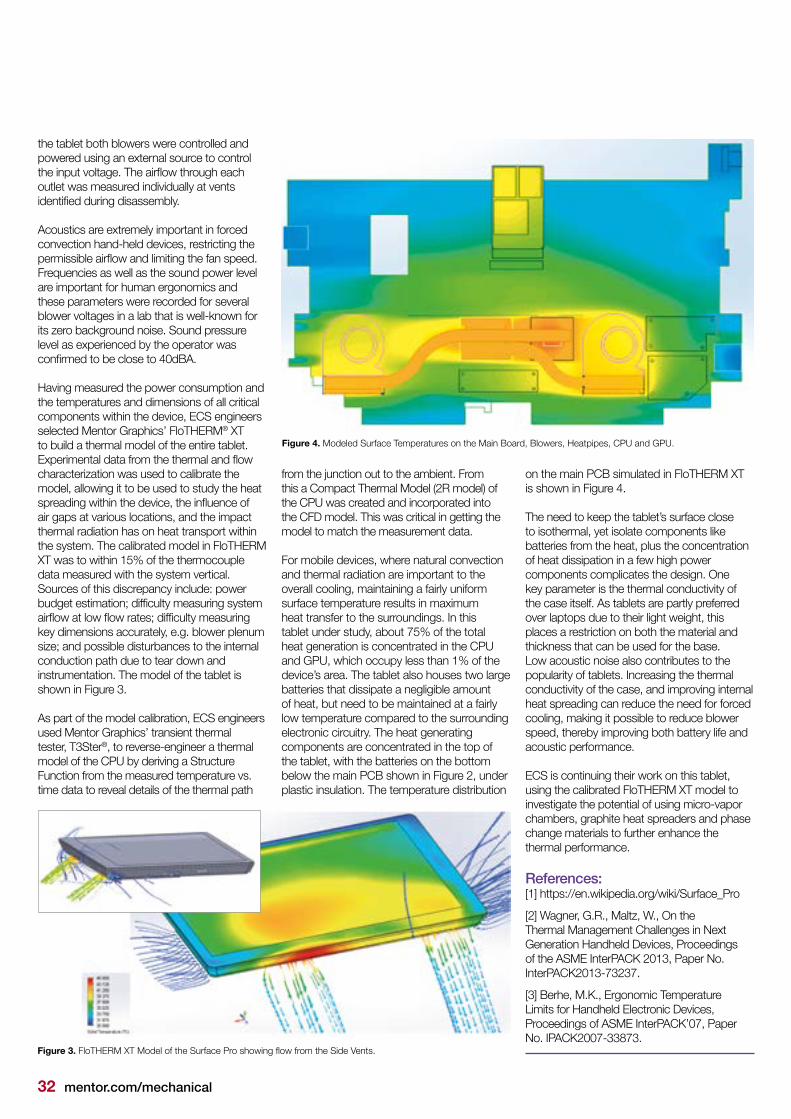
32 mentor.com/mechanical
the tablet both blowers were controlled and powered using an external source to control the input voltage. The airflow through each outlet was measured individually at vents identified during disassembly.
Acoustics are extremely important in forced convection hand-held devices, restricting the permissible airflow and limiting the fan speed. Frequencies as well as the sound power level are important for human ergonomics and these parameters were recorded for several blower voltages in a lab that is well-known for its zero background noise. Sound pressure level as experienced by the operator was confirmed to be close to 40dBA.
Having measured the power consumption and the temperatures and dimensions of all critical components within the device, ECS engineers selected Mentor Graphics’ FloTHERM® XT to build a thermal model of the entire tablet. Experimental data from the thermal and flow characterization was used to calibrate the model, allowing it to be used to study the heat spreading within the device, the influence of air gaps at various locations, and the impact thermal radiation has on heat transport within the system. The calibrated model in FloTHERM XT was to within 15% of the thermocouple data measured with the system vertical. Sources of this discrepancy include: power budget estimation; difficulty measuring system airflow at low flow rates; difficulty measuring key dimensions accurately, e.g. blower plenum size; and possible disturbances to the internal conduction path due to tear down and instrumentation. The model of the tablet is shown in Figure 3.
As part of the model calibration, ECS engineers used Mentor Graphics’ transient thermal tester, T3Ster®, to reverse-engineer a thermal model of the CPU by deriving a Structure Function from the measured temperature vs. time data to reveal details of the thermal path
from the junction out to the ambient. From this a Compact Thermal Model (2R model) of the CPU was created and incorporated into the CFD model. This was critical in getting the model to match the measurement data.
For mobile devices, where natural convection and thermal radiation are important to the overall cooling, maintaining a fairly uniform surface temperature results in maximum heat transfer to the surroundings. In this tablet under study, about 75% of the total heat generation is concentrated in the CPU and GPU, which occupy less than 1% of the device’s area. The tablet also houses two large batteries that dissipate a negligible amount of heat, but need to be maintained at a fairly low temperature compared to the surrounding electronic circuitry. The heat generating components are concentrated in the top of the tablet, with the batteries on the bottom below the main PCB shown in Figure 2, under plastic insulation. The temperature distribution
on the main PCB simulated in FloTHERM XT is shown in Figure 4.
The need to keep the tablet’s surface close to isothermal, yet isolate components like batteries from the heat, plus the concentration of heat dissipation in a few high power components complicates the design. One key parameter is the thermal conductivity of the case itself. As tablets are partly preferred over laptops due to their light weight, this places a restriction on both the material and thickness that can be used for the base. Low acoustic noise also contributes to the popularity of tablets. Increasing the thermal conductivity of the case, and improving internal heat spreading can reduce the need for forced cooling, making it possible to reduce blower speed, thereby improving both battery life and acoustic performance.
ECS is continuing their work on this tablet, using the calibrated FloTHERM XT model to investigate the potential of using micro-vapor chambers, graphite heat spreaders and phase change materials to further enhance the thermal performance.
References:[1] https://en.wikipedia.org/wiki/Surface_Pro
[2] Wagner, G.R., Maltz, W., On the Thermal Management Challenges in Next Generation Handheld Devices, Proceedings of the ASME InterPACK 2013, Paper No. InterPACK2013-73237.
[3] Berhe, M.K., Ergonomic Temperature Limits for Handheld Electronic Devices, Proceedings of ASME InterPACK’07, Paper No. IPACK2007-33873.
Figure 4. Modeled Surface Temperatures on the Main Board, Blowers, Heatpipes, CPU and GPU.
Figure 3. FloTHERM XT Model of the Surface Pro showing flow from the Side Vents.

mentor.com/mechanical 33
Design Processes and Levels of Thermal AnalysisDesign Processes and Levels of Thermal Analysis at United Automotive Electronics Systems Co. Ltd. (UAES)By Boris Marovic, Product Market Manager, Mentor Graphics
At UAES, a Robert Bosch company, the thermal simulation of products takes an increasing role in the
product development process. In a joint venture with Chinese Engine Management Systems Corporation Ltd (CNEMS), the product line includes a large range of automotive powertrain components such as Engine/Electronic Control Units (ECUs), Sensors, Ignition Coils, Inverters and Throttle Valves. The increasing demand in thermal management requires a recognition of the product development process and the introduction of an increased number of simulation steps, in order to ensure product functionality, performance, and reliability.
At UAES’ Technical Product Development Center, the CAE Manager Bao Chenyu, and his team ensures the thermal performance of their products is within the limitation of the components and customers' specifications. The application of FloEFD™ and FloTHERM® increases the breadth of the simulation capabilities from early in the design stage, to the start of production (SOP). Both tools are used either separately or in combination, depending on the level of thermal analysis.
Starting at Level 1, UAES uses FloTHERM for any calculation of temperature increase in the chip design. Followed by Level 2, where both FloEFD and FloTHERM are applied depending on the depth of design
A
stage, and need for an electronic cooling specific functionality. The calculation of chip configurations and improvements in cooling measures at level 2 can be very detailed and requires the consideration of the copper traces, vias and the correct thermal modeling of the chips.
In Level 3, assemblies can often get more complex and require the inclusion of their housings and the environment
they work in. Here the thermal analysis applications include ECUs, PEUs (Power Electronic Units), batteries and many more components.
Levels 4 and 5 are executed in system modeling tools.
Back at level 3, and looking more closely at the application in an ignition coil and PEU, we can see that the detail of the simulation
Figure 1. Levels of Thermal Analysis and Application Area
Automotive
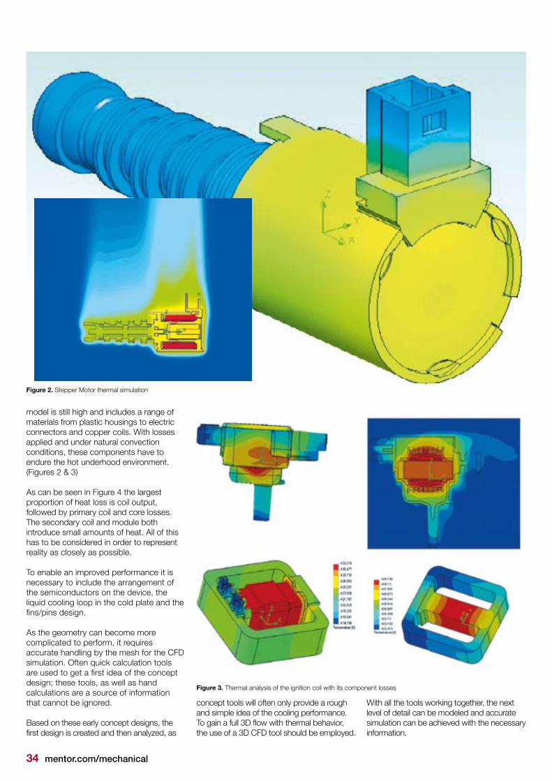
34 mentor.com/mechanical
model is still high and includes a range of materials from plastic housings to electric connectors and copper coils. With losses applied and under natural convection conditions, these components have to endure the hot underhood environment. (Figures 2 & 3)
As can be seen in Figure 4 the largest proportion of heat loss is coil output, followed by primary coil and core losses. The secondary coil and module both introduce small amounts of heat. All of this has to be considered in order to represent reality as closely as possible.
To enable an improved performance it is necessary to include the arrangement of the semiconductors on the device, the liquid cooling loop in the cold plate and the fins/pins design.
As the geometry can become more complicated to perform, it requires accurate handling by the mesh for the CFD simulation. Often quick calculation tools are used to get a first idea of the concept design; these tools, as well as hand calculations are a source of information that cannot be ignored.
Based on these early concept designs, the first design is created and then analyzed, as
Figure 2. Stepper Motor thermal simulation
Figure 3. Thermal analysis of the ignition coil with its component losses
concept tools will often only provide a rough and simple idea of the cooling performance. To gain a full 3D flow with thermal behavior, the use of a 3D CFD tool should be employed.
With all the tools working together, the next level of detail can be modeled and accurate simulation can be achieved with the necessary information.
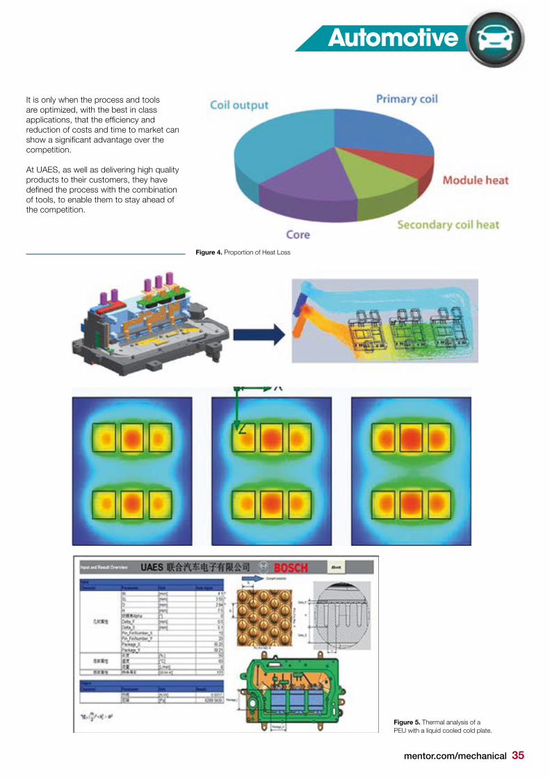
mentor.com/mechanical 35
It is only when the process and tools are optimized, with the best in class applications, that the efficiency and reduction of costs and time to market can show a significant advantage over the competition.
At UAES, as well as delivering high quality products to their customers, they have defined the process with the combination of tools, to enable them to stay ahead of the competition.
Figure 5. Thermal analysis of a PEU with a liquid cooled cold plate.
Figure 4. Proportion of Heat Loss
Automotive
Figure 3. Thermal analysis of the ignition coil with its component losses
mentor.com/mechanical 37
he traditional development of aircraft of any type usually goes through a long design process until the first full-scale
prototype is built to test flight behavior. Such an approach is extremely costly considering the capital investment required for large passenger liners. Considering the challenges faced by the recent development of the Airbus A380 and Boeing 787 Dreamliner, manufacturers and component suppliers are understandably under increased pressure to deliver right, on time, every time.
There is therefore a need to streamline the development process and improve the prediction accuracy in flight behaviors in real-time flight simulators. Dr. Olivares and his team at the National Institute for Aviation Research (NIAR) of the Wichita State University set out to develop a method to increase the prediction accuracy of flight behaviors with the real-time flight simulator, MIURA. Conventional aerodynamic calculations used by the simulator were not accurate enough, especially predicting stall and other effects such as propeller performance or the wing-fuselage interference. The NIAR team conducted several simulations with Mentor Graphics’ FloEFD™ Simulation Software on their test model, a push propeller UAV (Figure 1), in order to get more accurate data to feed into the simulator for a better prediction of flight characteristics as well as to validate the FloEFD results with wind tunnel measurements.
T
Aerospace
Up, Up and Away!Using CFD tools to develop a Real-Time Flight Model
By Gerardo Olivares Ph.D.; A. Barragan; J. M. Gomez; and H. Solano, National Institute for Aviation Research
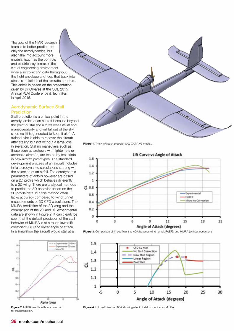
38 mentor.com/mechanical
The goal of the NIAR research team is to better predict, not only the aerodynamics, but also take into account more models, (such as the controls and electrical systems), in the virtual engineering environment while also collecting data throughout the flight envelope and feed that back into stress simulations of the aircrafts structure. This article is based on the presentation given by Dr Olivares at the COE 2015 Annual PLM Conference & TechniFair in April 2015.
Aerodynamic Surface Stall PredictionStall prediction is a critical point in the aerodynamics of an aircraft because beyond the point of stall the aircraft loses its lift and maneuverability and will fall out of the sky since no lift is generated to keep it aloft. A trained pilot is able to recover the aircraft after stalling but not without a large loss in elevation. Stalling maneuvers such as those seen at airshows with fighter jets or acrobatic aircrafts, are tested by test pilots in new aircraft prototypes. The standard development process of an aircraft includes initial aerodynamic calculations starting with the selection of an airfoil. The aerodynamic parameters of airfoils however are based on a 2D profile which behaves differently to a 3D wing. There are analytical methods to predict the 3D behavior based on the 2D profile data, but this method often lacks accuracy compared to wind tunnel measurements or 3D CFD calculations. The MIURA prediction of the 3D wing and the comparison of the 2D and 3D experimental data are shown in Figure 2. It can clearly be seen that the default prediction of the stall behavior of MIURA is at a much lower lift coefficient (CL) and lower angle of attack.In a simulation the aircraft would stall at a
Figure 2. MIURA results without correction for stall prediction.
Figure 1. The NIAR push propeller UAV CATIA V5 model..
Figure 3. Comparison of lift coefficient vs AOA between wind tunnel, FloEFD and MIURA (without correction)
Figure 4. Lift coefficient vs. AOA showing effect of stall correction for MIURA

mentor.com/mechanical 39
much smaller angle and lower lift compared to the reality. The NIAR team built a 3D wing as an extrusion of the 2D airfoil SD7062 and measured its aerodynamic performance in the closed loop Beech Wind Tunnel at the Wichita State University (WSU). They then conducted a FloEFD simulation at a range of angles of attack (AOA).
The results from the experiment, FloEFD and MIURA (without correction) are shown in Figure 3 and shows that FloEFD has the same lift curve slope and stall pattern as the wind tunnel data. MIURA on the other hand captures the initial slope but over - predicts the stall at 17° AOA.
The vital parts of the lift curve that MIURA must correct are after the linear section so as not to over-predict the lift and drop too strongly after the maximum lift. In order to do that, MIURA enables the user to input the CLmax and an additional point after that, and consequently calculates the post-stall again on its own (Figure 4).
This method leads to a drastically improved stall behavior (Figure 5). The corrected MIURA calculation fits the stall behavior of the experimental data much better than the uncorrected calculation.
Propeller PerformanceSince the polars used in airfoils also apply for the propeller blades, the same problem affects the propeller performance and can be seen in the thrust and power coefficient vs. advance ratio of the propeller diagrams shown in Figure 6.
This is especially true in the crucial take-off and climb phase where the curves differ drastically and would result in extremely different flight behavior by the simulator.
Aerospace
Figure 5. Lift coefficient vs. AOA showing the corrected MIURA results compared to the experiments
Figure 6. Thrust and power coefficient prediction of MIURA compared to experimental data
Figure 7. Thrust and power coefficient (CT and CP respectively) comparison between wind tunnel, FloEFD and MIURA (not corrected)
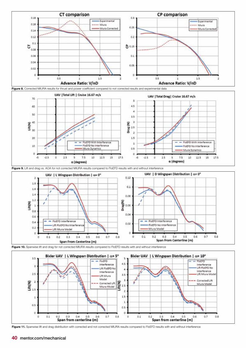
40 mentor.com/mechanical
Figure 8. Corrected MIURA results for thrust and power coefficient compared to not corrected results and experimental data
Figure 9. Lift and drag vs. AOA for not corrected MIURA results compared to FloEFD results with and without interference
Figure 11. Spanwise lift and drag distribution with corrected and not corrected MIURA results compared to FloEFD results with and without interference
Figure 10. Spanwise lift and drag for not corrected MIURA results compared to FloEFD results with and without interference
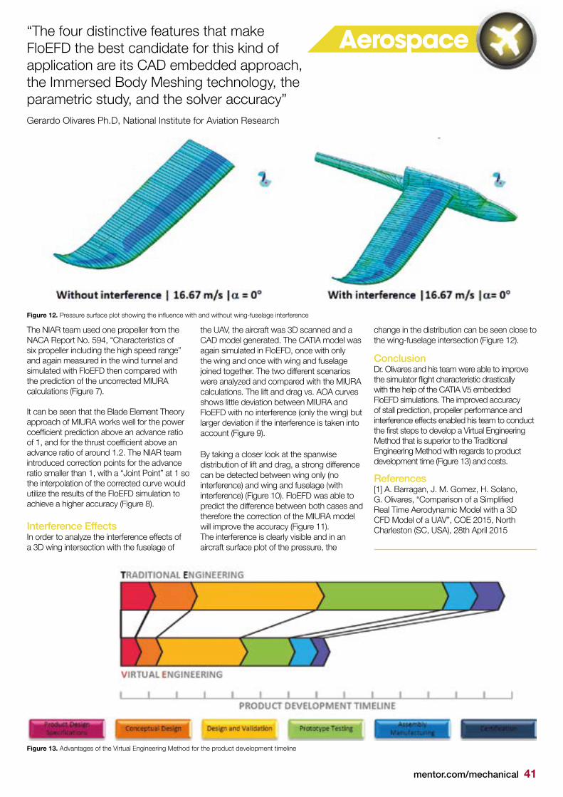
mentor.com/mechanical 41
Aerospace
The NIAR team used one propeller from the NACA Report No. 594, “Characteristics of six propeller including the high speed range” and again measured in the wind tunnel and simulated with FloEFD then compared with the prediction of the uncorrected MIURA calculations (Figure 7).
It can be seen that the Blade Element Theory approach of MIURA works well for the power coefficient prediction above an advance ratio of 1, and for the thrust coefficient above an advance ratio of around 1.2. The NIAR team introduced correction points for the advance ratio smaller than 1, with a “Joint Point” at 1 so the interpolation of the corrected curve would utilize the results of the FloEFD simulation to achieve a higher accuracy (Figure 8).
Interference EffectsIn order to analyze the interference effects of a 3D wing intersection with the fuselage of
the UAV, the aircraft was 3D scanned and a CAD model generated. The CATIA model was again simulated in FloEFD, once with only the wing and once with wing and fuselage joined together. The two different scenarios were analyzed and compared with the MIURA calculations. The lift and drag vs. AOA curves shows little deviation between MIURA and FloEFD with no interference (only the wing) but larger deviation if the interference is taken into account (Figure 9).
By taking a closer look at the spanwise distribution of lift and drag, a strong difference can be detected between wing only (no interference) and wing and fuselage (with interference) (Figure 10). FloEFD was able to predict the difference between both cases and therefore the correction of the MIURA model will improve the accuracy (Figure 11).The interference is clearly visible and in an aircraft surface plot of the pressure, the
change in the distribution can be seen close to the wing-fuselage intersection (Figure 12).
ConclusionDr. Olivares and his team were able to improve the simulator flight characteristic drastically with the help of the CATIA V5 embedded FloEFD simulations. The improved accuracy of stall prediction, propeller performance and interference effects enabled his team to conduct the first steps to develop a Virtual Engineering Method that is superior to the Traditional Engineering Method with regards to product development time (Figure 13) and costs.
References[1] A. Barragan, J. M. Gomez, H. Solano, G. Olivares, “Comparison of a Simplified Real Time Aerodynamic Model with a 3D CFD Model of a UAV”, COE 2015, North Charleston (SC, USA), 28th April 2015
Figure 12. Pressure surface plot showing the influence with and without wing-fuselage interference
Figure 13. Advantages of the Virtual Engineering Method for the product development timeline
“The four distinctive features that make FloEFD the best candidate for this kind of application are its CAD embedded approach, the Immersed Body Meshing technology, the parametric study, and the solver accuracy”Gerardo Olivares Ph.D, National Institute for Aviation Research
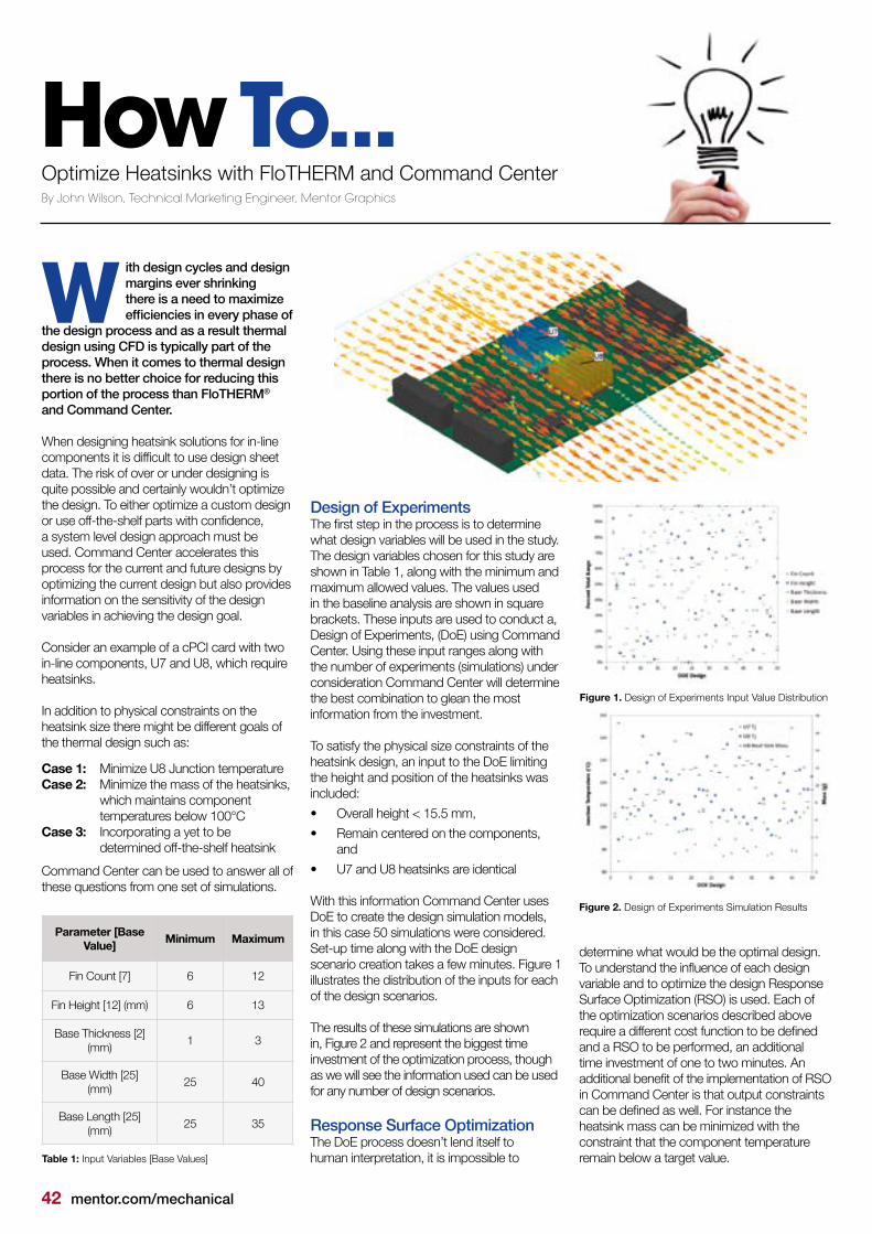
42 mentor.com/mechanical
How To...Optimize Heatsinks with FloTHERM and Command CenterBy John Wilson, Technical Marketing Engineer, Mentor Graphics
ith design cycles and design margins ever shrinking there is a need to maximize efficiencies in every phase of
the design process and as a result thermal design using CFD is typically part of the process. When it comes to thermal design there is no better choice for reducing this portion of the process than FloTHERM® and Command Center.
When designing heatsink solutions for in-line components it is difficult to use design sheet data. The risk of over or under designing is quite possible and certainly wouldn’t optimize the design. To either optimize a custom design or use off-the-shelf parts with confidence, a system level design approach must be used. Command Center accelerates this process for the current and future designs by optimizing the current design but also provides information on the sensitivity of the design variables in achieving the design goal.
Consider an example of a cPCI card with two in-line components, U7 and U8, which require heatsinks. In addition to physical constraints on the heatsink size there might be different goals of the thermal design such as:
Case 1: Minimize U8 Junction temperature Case 2: Minimize the mass of the heatsinks,
which maintains component temperatures below 100°C
Case 3: Incorporating a yet to be determined off-the-shelf heatsink
Command Center can be used to answer all of these questions from one set of simulations.
W
Design of ExperimentsThe first step in the process is to determine what design variables will be used in the study. The design variables chosen for this study are shown in Table 1, along with the minimum and maximum allowed values. The values used in the baseline analysis are shown in square brackets. These inputs are used to conduct a, Design of Experiments, (DoE) using Command Center. Using these input ranges along with the number of experiments (simulations) under consideration Command Center will determine the best combination to glean the most information from the investment. To satisfy the physical size constraints of the heatsink design, an input to the DoE limiting the height and position of the heatsinks was included:
• Overall height < 15.5 mm,
• Remain centered on the components, and
• U7 and U8 heatsinks are identical With this information Command Center uses DoE to create the design simulation models, in this case 50 simulations were considered. Set-up time along with the DoE design scenario creation takes a few minutes. Figure 1 illustrates the distribution of the inputs for each of the design scenarios. The results of these simulations are shown in, Figure 2 and represent the biggest time investment of the optimization process, though as we will see the information used can be used for any number of design scenarios.
Response Surface Optimization The DoE process doesn’t lend itself to human interpretation, it is impossible to
determine what would be the optimal design. To understand the influence of each design variable and to optimize the design Response Surface Optimization (RSO) is used. Each of the optimization scenarios described above require a different cost function to be defined and a RSO to be performed, an additional time investment of one to two minutes. An additional benefit of the implementation of RSO in Command Center is that output constraints can be defined as well. For instance the heatsink mass can be minimized with the constraint that the component temperature remain below a target value.
Figure 1. Design of Experiments Input Value Distribution
Figure 2. Design of Experiments Simulation Results
Parameter [Base Value]
Minimum Maximum
Fin Count [7] 6 12
Fin Height [12] (mm) 6 13
Base Thickness [2] (mm)
1 3
Base Width [25] (mm)
25 40
Base Length [25] (mm)
25 35
Table 1: Input Variables [Base Values]
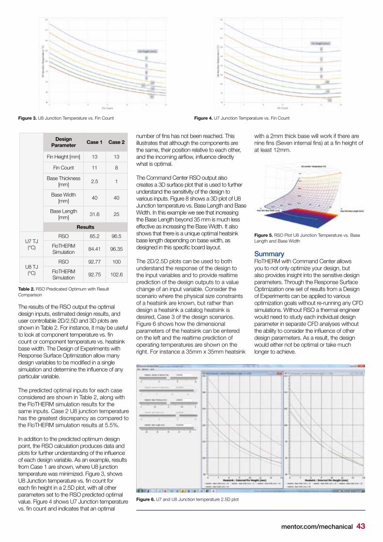
mentor.com/mechanical 43
with a 2mm thick base will work if there are nine fins (Seven internal fins) at a fin height of at least 12mm.
The results of the RSO output the optimal design inputs, estimated design results, and user controllable 2D/2.5D and 3D plots are shown in Table 2. For instance, it may be useful to look at component temperature vs. fin count or component temperature vs. heatsink base width. The Design of Experiments with Response Surface Optimization allow many design variables to be modified in a single simulation and determine the influence of any particular variable.
The predicted optimal inputs for each case considered are shown in Table 2, along with the FloTHERM simulation results for the same inputs. Case 2 U8 junction temperature has the greatest discrepancy as compared to the FloTHERM simulation results at 5.5%.
In addition to the predicted optimum design point, the RSO calculation produces data and plots for further understanding of the influence of each design variable. As an example, results from Case 1 are shown, where U8 junction temperature was minimized. Figure 3, shows U8 Junction temperature vs. fin count for each fin height in a 2.5D plot, with all other parameters set to the RSO predicted optimal value. Figure 4 shows U7 Junction temperature vs. fin count and indicates that an optimal
number of fins has not been reached. This illustrates that although the components are the same, their position relative to each other, and the incoming airflow, influence directly what is optimal.
The Command Center RSO output also creates a 3D surface plot that is used to further understand the sensitivity of the design to various inputs. Figure 8 shows a 3D plot of U8 Junction temperature vs. Base Length and Base Width. In this example we see that increasing the Base Length beyond 35 mm is much less effective as increasing the Base Width. It also shows that there is a unique optimal heatsink base length depending on base width, as designed in this specific board layout.
The 2D/2.5D plots can be used to both understand the response of the design to the input variables and to provide realtime prediction of the design outputs to a value change of an input variable. Consider the scenario where the physical size constraints of a heatsink are known, but rather than design a heatsink a catalog heatsink is desired, Case 3 of the design scenarios. Figure 6 shows how the dimensional parameters of the heatsink can be entered on the left and the realtime prediction of operating temperatures are shown on the right. For instance a 35mm x 35mm heatsink
Design Parameter
Case 1 Case 2
Fin Height [mm] 13 13
Fin Count 11 8
Base Thickness [mm]
2.5 1
Base Width [mm]
40 40
Base Length [mm]
31.6 25
Results
U7 TJ (°C)
RSO 85.2 96.5
FloTHERM Simulation
84.41 96.35
U8 TJ (°C)
RSO 92.77 100
FloTHERM Simulation
92.75 102.6
Table 2. RSO Predicated Optimum with Result Comparison
Figure 5. RSO Plot U8 Junction Temperature vs. Base Length and Base Width
Figure 6. U7 and U8 Junction temperature 2.5D plot
Figure 3. U8 Junction Temperature vs. Fin Count Figure 4. U7 Junction Temperature vs. Fin Count
SummaryFloTHERM with Command Center allows you to not only optimize your design, but also provides insight into the sensitive design parameters. Through the Response Surface Optimization one set of results from a Design of Experiments can be applied to various optimization goals without re-running any CFD simulations. Without RSO a thermal engineer would need to study each individual design parameter in separate CFD analyses without the ability to consider the influence of other design pararmeters. As a result, the design would either not be optimal or take much longer to achieve.
44 mentor.com/mechanical
Interview
Koen Beyers has a Bachelors and Masters’ degrees in Product Development from Loughborough University, UK and Hogeschool Antwerpen respectively and 17 years of experience in product design and simulation. He is the founder of Voxdale located in Wijnegem, Belgium and is a co-founder and CTO of Novosanis. Prior to founding Voxdale, Koen worked as a Senior Mechanical Engineer at Barco Projection Systems. He has won numerous awards for his designs and is recognized as an innovator in industry.
Q: Tell us about Voxdale and what your company does?A: Voxdale is a design engineering agency, we sell services to customers who lack general R&D or want to start new innovation project but do not have the right resources to do so. We have a really diverse client base. Voxdale was established in 2005 and from the very beginning of the company we utilized simulation tools. We believe that early feasibility studies of concepts through simulation can prove or disprove ideas quickly, and counteract arguments that things won’t work or can’t be done. This approach allows us to take what sometimes seems like crazy ideas but to do a quick check to see if they work with simulation. You can do this within two to three days with simulation rather than two to three months of experimentation.
Q: What would you say are Voxdale’s core strengths?A: We are design engineering experts, which makes us different from pure simulation companies. While we get simulation work only, we will also provide sets of design recommendations for improvements as we are, in our minds, designers. We explain that our goal is the final solution with proof of what can be done to optimize the design or show how it is wrong.
In our hearts we are designers and this is my philosophy behind the company.
in the software and ten years ago I was convinced that we would be doing everything with simulation by now. Although simulation tools are better and faster, I kind of believe the opposite. We are now also using the other tools that make developments more fun. Tools for 3D printing allow for quick mock-ups, enable us to search for the correlation between what we predict with simulation and what we can prove with the wind tunnels. So we have moved to the opposite of everything digital, as I thought ten years ago. At first I thought this was because the customers believed that this would be too risky, but now it is just a very flexible way of working and using all the tools available. So it is a mixture between the two technologies, which I see as staying the same for the next 20 years.
Q: How have those changes impacted your business?A: Testing facilities – much more than we thought. We thought we would be investing only in software and fast computers, but actually we are spending more on testing capabilities. But simulation is still a key tool that we use. Without the simulation aspect, my business would not be as it is now.
Q: What industry sectors do you see that could benefit the most from simulation?A: The sector toughest to get into and the one that could benefit the most is the processing industry. These are heavy industries who cannot stop production lines and experiment with the processes even though a 3% change in performance can mean millions of dollars in savings.
Q: Where do you see CFD going in your business in the future? A: I have been working with FloEFD for ten years. It was the first simulation tool I bought. My fear from day one was it’s a nice tool but it's embedded and saw software providers giving embedded tools for free to all CAD users. I thought this would kill that part of my business, but it hasn’t. It must be the combination of our expertise in simulation and our tools to prove and correlate that the simulation is correct. I believe it will always be a big part of our business. It is one of our core competencies. We must take care as we grow with the tool. It is a bit dangerous to be too high-end, but not too mainstream which does not fit our business model. I guess then the complexity of projects and systems will increase. It must be a self-balancing system. Things get smaller, higher performing, and smarter. This high-end push will allow us to continue our approach. CFD will always be at the core of our simulation capabilites.
Q: Who do you work with?A: We work with a lot of small companies. I am always surprised by how much innovation and R&D there is occurring in Flanders (Belgium). These companies have small R&D teams and cannot justify buying simulation licenses themselves. 50 - 60% of our work is with these small companies who want R&D assistance or want thermal optimization or material selection. We have to work quickly to provide solutions usually within weeks not months.
Geographically, there are not a lot of big companies in Belgium, but we do also work for some big companies who like our expertise and philosophy. Typically we only have a small piece of the R&D work. Usually one specific thing that they don’t want to focus on themselves, for example, the simulation part.
Q: How do you choose which types of projects you want to get involved with?A: We work with companies that are too small to have their own R&D teams or large companies that have a philosophy of outsourcing work that is not in their core competencies.
It's hard to say no to work, but if we feel there is no match with our capabilities we will say as we don’t want to go through the pain but it is hard, we like to stretch ourselves.
Q: Which project, that, Voxdale has been involved with, are you most proud of?A: There are some quite spectacular projects that I am proud of like the Bernico F2 boat that broke the world speed record or the Indy Car project with Conquest Racing. Another project I am proud of is the QARMAN satellite where we worked with Von Karman Institute to optimize the architecture of the QARMAN Cube satellite.
Q: Voxdale uses simulation as part of their frontloaded design process. Can you talk about your philosophy around upfront simulation?A: We use simulation as a first step in the design process when we have a new design project. When we collate all specifications, we like to be very broad in our brainstorming. We start with a simple model rather than a complex model that has a lot of detail. At this point we can take a lot of design risks trying to learn something from it. It might not work the first time but as long as you learn from it you are making progress. So we rely heavily on simulation early on in these projects.
Q: In the time that you have been involved in simulation, what are the biggest changes that you have seen?A: The obvious changes are technological, a lot more computation power and functionality
Koen Beyers, Voxdale BVBA
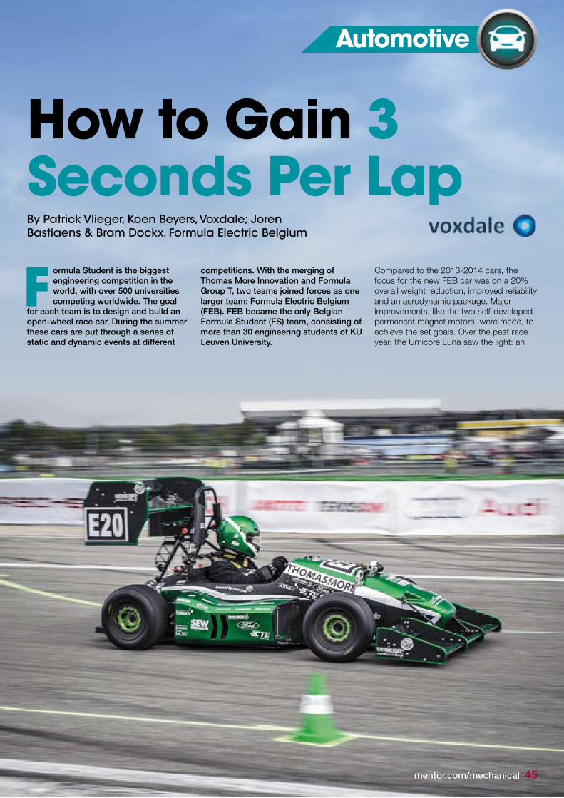
Automotive
How to Gain 3 Seconds Per LapBy Patrick Vlieger, Koen Beyers, Voxdale; Joren Bastiaens & Bram Dockx, Formula Electric Belgium
ormula Student is the biggest engineering competition in the world, with over 500 universities competing worldwide. The goal
for each team is to design and build an open-wheel race car. During the summer these cars are put through a series of static and dynamic events at different
competitions. With the merging of Thomas More Innovation and Formula Group T, two teams joined forces as one larger team: Formula Electric Belgium (FEB). FEB became the only Belgian Formula Student (FS) team, consisting of more than 30 engineering students of KU Leuven University.
Compared to the 2013-2014 cars, the focus for the new FEB car was on a 20% overall weight reduction, improved reliability and an aerodynamic package. Major improvements, like the two self-developed permanent magnet motors, were made, to achieve the set goals. Over the past race year, the Umicore Luna saw the light: an
F
mentor.com/mechanical 45

46 mentor.com/mechanical
electric FS race car, with a weight of 208 kg and an acceleration to 100 km/h in just 2.7 seconds!
The Umicore Luna was also set out to be the first Belgian FS car to feature a fully developed aerodynamic package, consisting of a front wing, diffuser, and rear wing. The package was to be added to the Umicore Luna to generate a higher amount of downforce with the aim of achieving higher cornering speeds on the track. The research on this topic was completed in the context of a Master’s Thesis to obtain a degree in Industrial Engineering in Electromechanics. During the design of this aero package, the students were supported by Belgian design, engineering and research company, Voxdale bvba.
Voxdale specialize in automotive, medical and industrial sectors, as well as space
Thomas More Innova.on Formula Group T Formula Electric Belgium
Car Name UTM-‐2 June Umicore Luna
Year 2014 2014 2015
Weight [kg] 290 240 208
Accelera.on 0-‐100 km/h [sec]
< 4 3.0 2.7
LiG coefficient \ 0.098 -‐1.200
Drag coefficient \ 0.456 0.545
Body Steel tubular spaceframe with flax fiber body
Carbon-‐fiber-‐reinforced polymer (CFRP) monocoque
Carbon-‐fiber-‐reinforced polymer (CFRP) monocoque
and aerospace industries. In its design and engineering process, Voxdale uses FloEFD™ for the optimization of designs. Most recently it has been used in drag reduction of trucks and Indycar race cars, as well as for structural analyses and thermal management projects.
Together with Voxdale the students came up with a plan of action, with weekly progress meetings.
The design of the aero package for the race car started out with the search for an airfoil for the front and rear wing, suitable for the needs of the Formula Student competition. Since the average speed of a Formula Student car is relatively low, an ideal high lift and low Reynolds airfoil was chosen. As a result of the gain in downforce and overall efficiency of the wing, a two-stage wing was chosen.
The angle of attack, gap and overhang of both wing stages were simulated in 2D. A manual mesh dependency test was performed successfully for the 2D wing and showed a steady result around 1.25 million cells. Using the Automatic Refinement option in FloEFD, the number of cells dropped to 250,000, resulting in an enormous reduction of calculation time, while still obtaining correct results.
The parameter for this optimization was to obtain the highest possible square lift coefficient, while minimizing the drag coefficient (max CL²/CD). Over 100 simulations were performed to obtain the best value.
The angle of the diffuser was simulated in the same way: different angles were simulated in 2D, while numerous diffuser lengths were observed in 3D. The pitch of
Figure 1. Model history of Formula Student cars
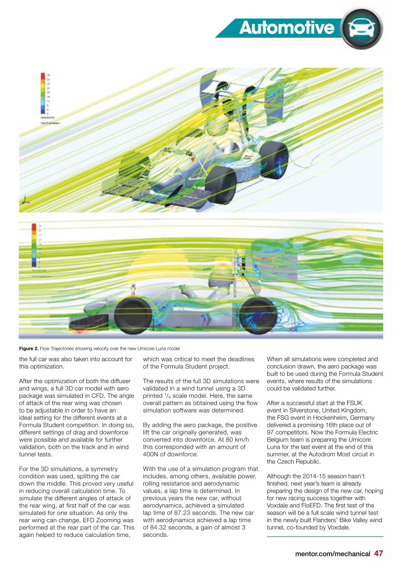
mentor.com/mechanical 47
the full car was also taken into account for this optimization.
After the optimization of both the diffuser and wings, a full 3D car model with aero package was simulated in CFD. The angle of attack of the rear wing was chosen to be adjustable in order to have an ideal setting for the different events at a Formula Student competition. In doing so, different settings of drag and downforce were possible and available for further validation, both on the track and in wind tunnel tests.
For the 3D simulations, a symmetry condition was used, splitting the car down the middle. This proved very useful in reducing overall calculation time. To simulate the different angles of attack of the rear wing, at first half of the car was simulated for one situation. As only the rear wing can change, EFD Zooming was performed at the rear part of the car. This again helped to reduce calculation time,
which was critical to meet the deadlines of the Formula Student project.
The results of the full 3D simulations were validated in a wind tunnel using a 3D printed 1/8 scale model. Here, the same overall pattern as obtained using the flow simulation software was determined.
By adding the aero package, the positive lift the car originally generated, was converted into downforce. At 80 km/h this corresponded with an amount of 400N of downforce.
With the use of a simulation program that includes, among others, available power, rolling resistance and aerodynamic values, a lap time is determined. In previous years the new car, without aerodynamics, achieved a simulated lap time of 87.23 seconds. The new car with aerodynamics achieved a lap time of 84.32 seconds, a gain of almost 3 seconds.
When all simulations were completed and conclusion drawn, the aero package was built to be used during the Formula Student events, where results of the simulations could be validated further.
After a successful start at the FSUK event in Silverstone, United Kingdom, the FSG event in Hockenheim, Germany delivered a promising 16th place out of 97 competitors. Now the Formula Electric Belgium team is preparing the Umicore Luna for the last event at the end of this summer, at the Autodrom Most circuit in the Czech Republic.
Although the 2014-15 season hasn’t finished, next year’s team is already preparing the design of the new car, hoping for new racing success together with Voxdale and FloEFD. The first test of the season will be a full scale wind tunnel test in the newly built Flanders’ Bike Valley wind tunnel, co-founded by Voxdale.
Automotive
Figure 2. Flow Trajectories showing velocity over the new Umicore Luna model
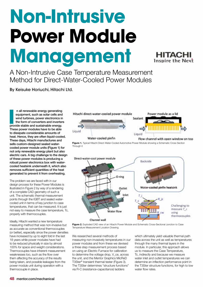
48 mentor.com/mechanical
By Keisuke Horiuchi, Hitachi Ltd.
n all renewable energy generating equipment, such as solar cells and wind turbines, power electronics in the form of converters and inverters
provide stable and sustainable energy. These power modules have to be able to dissipate considerable amounts of heat. Hence, they are often liquid-cooled. These days, Hitachi manufactures and sells custom-designed sealed water-cooled power module units (Figure 1) for not only renewable energy plant but also electric cars. A big challenge to the design of these power modules is producing a robust power electronics box with water-cooled heatsink underneath it, which also removes sufficient quantities of the heat generated to prevent it from overheating.
The problem we are faced with in our design process for these Power Modules is illustrated in Figure 2 by way of a rendering of a complete CAD geometry of such a unit. The schematic thermal measurement points through the IGBT and sealed water-cooled unit in terms of key junction to case temperatures, that can be measured. It is just not easy to measure the case temperature, Tc, properly with thermocouples.
Ideally, Hitachi wanted a new temperature measuring method that was non-invasive but as accurate as conventional thermocouples (or better), especially since the power densities have increased by up to eight fold in the last 18 years while power modules have had to be reduced physically in size by almost 100% for space and weight considerations. Thermocouples have inherent measurement weaknesses too, such as the flow over them affecting the accuracy of the results being taken, and possible leakages from the power module unit during operation with a thermocouple in place.
I
We researched several methods of measuring non-invasively temperatures in our power modules and from these we devised a three step measurement process based on using an Electric Furnace for calibration to determine the voltage drop, V_ce, across the unit, and the Mentor Graphics MicReD T3Ster® transient thermal tester (Figure 3). The T3Ster determines “structure functions” via R-C (resistance-capacitance) ladders
which ultimately yield valuable thermal path data across the unit as well as temperatures through the many thermal layers in the module. In particular, this approach allows us to measure the Case Temperature, Tc, indirectly and because we measure water inlet and outlet temperatures we can determine an inflection performance point in the T3Ster structure functions, for high to low water flow rates.
Figure 1. Typical Hitachi Direct-Water-Cooled Automotive Power Module showing a Schematic Cross Section Through it
Figure 2. Exploded CAD view of an Hitachi Power Module and Schematic Cross-Sectional Junction to Case Temperature Measurement Location Drawing.
Non-Intrusive Power Module ManagementA Non-Intrusive Case Temperature Measurement Method for Direct-Water-Cooled Power Modules
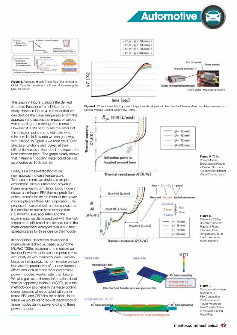
mentor.com/mechanical 49
The graph in Figure 5 shows the derived Structure Functions from T3Ster for the study shown in Figure 4. It is clear that we can deduce the Case Temperature from this approach and assess the impact of various water cooling rates through the module. However, it is still hard to see the details of the inflection point and to estimate what minimum liquid flow rate we can get away with. Hence, in Figure 6 we took the T3Ster structure functions and looked at their differential values in finer detail to pinpoint the best inflection point. The graph clearly shows that 7 litres/min. cooling water could be just as effective as 10 litres/min.
Finally, as a cross-verification of our new approach to case temperature, Tc, measurement, we devised a simple experiment using our tried-and-proven in-house engineering simulation tools. Figure 7 shows an in-house FEA thermal prediction of heat transfer inside the metal of the power module plate for three IGBTs operating. The proposed measurement method shows that it is possible to obtain case temperature (Tc) non-intrusive, accurately and the experimental results agreed well with the FEA temperature differential predictions, inside the metal component averaged over a 45° heat spreading area for three dies on the module. In conclusion, Hitachi has developed a non-invasive technique, based around the MicReD T3Ster equipment, to measure our Inverter Power Module case temperatures as accurately as with thermocouples. Crucially, because the approach is non-invasive we can increase the productivity of our development efforts and look at many more customized power modules, weeks faster than before. We also gain extra thermal information about what is happening inside our IGBTs, plus the methodology also helps in the water-cooling design process when coupled with our in-house FEA and CFD simulation tools. In the future we would like to look at diagnostics of failure modes during power cycling of these power modules.
Figure 3. Proposed Hitachi Three Step Test Method to Obtain Case Temperatures in a Power Module using the MicReD T3Ster
Figure 4. T3Ster-based Test Equipment Layout we developed with the Resultant Temperature Drop Measurements for Several Module Cooling Water Flow Rates
Figure 5. T3Ster Power Module Experimental Results – Derived Structure Functions for different Water-Cooling rates
Figure 6. Differential T3Ster Structure Function Replot of Figure 5 to Yield Case Temperature, Tc, in the Experimental Measurements
Figure 7. Comparison between Numerical 3D FEA Conduction Predictions and T3Ster Measured Heat Transfer Rates in the IGBT Cooled Metal Plate
Automotive
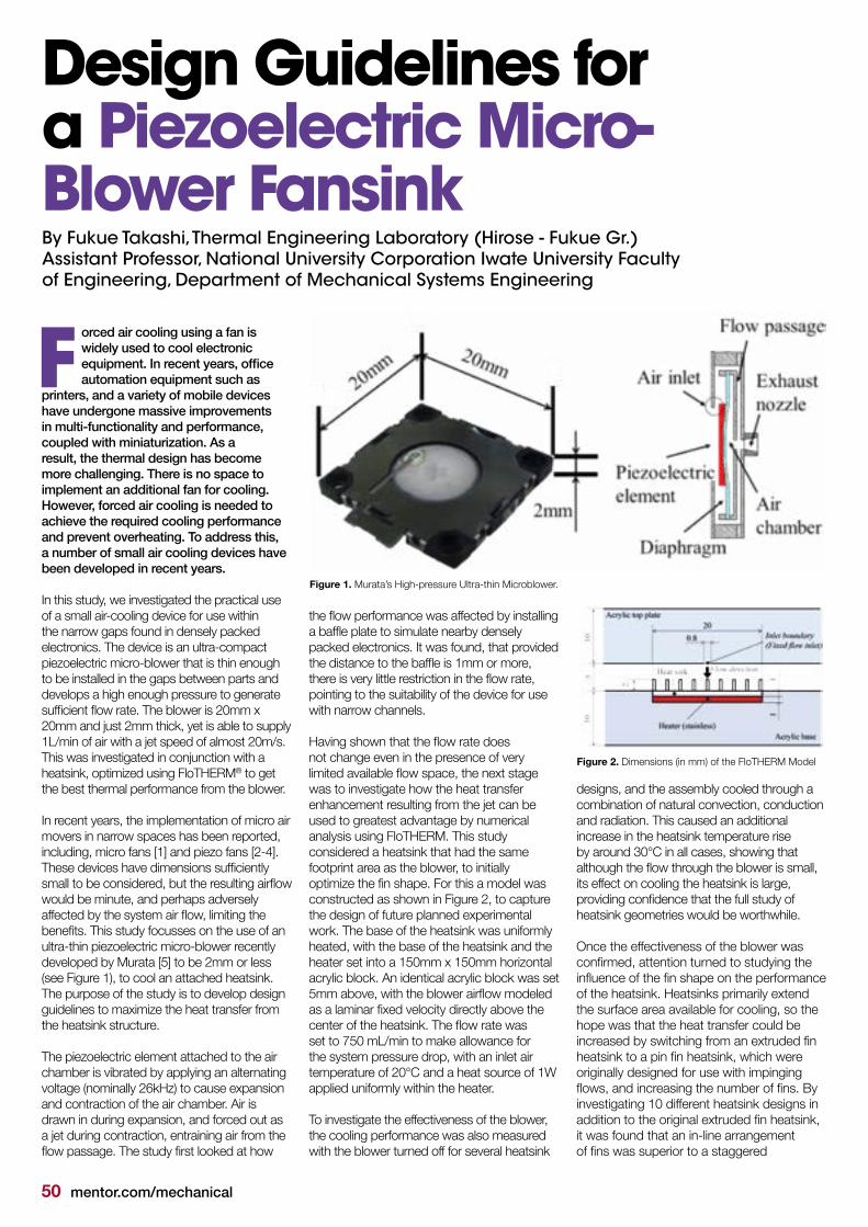
50 mentor.com/mechanical
Figure 1. Murata’s High-pressure Ultra-thin Microblower.
Figure 2. Dimensions (in mm) of the FloTHERM Model
orced air cooling using a fan is widely used to cool electronic equipment. In recent years, office automation equipment such as
printers, and a variety of mobile devices have undergone massive improvements in multi-functionality and performance, coupled with miniaturization. As a result, the thermal design has become more challenging. There is no space to implement an additional fan for cooling. However, forced air cooling is needed to achieve the required cooling performance and prevent overheating. To address this, a number of small air cooling devices have been developed in recent years.
In this study, we investigated the practical use of a small air-cooling device for use within the narrow gaps found in densely packed electronics. The device is an ultra-compact piezoelectric micro-blower that is thin enough to be installed in the gaps between parts and develops a high enough pressure to generate sufficient flow rate. The blower is 20mm x 20mm and just 2mm thick, yet is able to supply 1L/min of air with a jet speed of almost 20m/s. This was investigated in conjunction with a heatsink, optimized using FloTHERM® to get the best thermal performance from the blower.
In recent years, the implementation of micro air movers in narrow spaces has been reported, including, micro fans [1] and piezo fans [2-4]. These devices have dimensions sufficiently small to be considered, but the resulting airflow would be minute, and perhaps adversely affected by the system air flow, limiting the benefits. This study focusses on the use of an ultra-thin piezoelectric micro-blower recently developed by Murata [5] to be 2mm or less (see Figure 1), to cool an attached heatsink. The purpose of the study is to develop design guidelines to maximize the heat transfer from the heatsink structure.
The piezoelectric element attached to the air chamber is vibrated by applying an alternating voltage (nominally 26kHz) to cause expansion and contraction of the air chamber. Air is drawn in during expansion, and forced out as a jet during contraction, entraining air from the flow passage. The study first looked at how
F
Design Guidelines for a Piezoelectric Micro-Blower FansinkBy Fukue Takashi, Thermal Engineering Laboratory (Hirose - Fukue Gr.) Assistant Professor, National University Corporation Iwate University Faculty of Engineering, Department of Mechanical Systems Engineering
the flow performance was affected by installing a baffle plate to simulate nearby densely packed electronics. It was found, that provided the distance to the baffle is 1mm or more, there is very little restriction in the flow rate, pointing to the suitability of the device for use with narrow channels.
Having shown that the flow rate does not change even in the presence of very limited available flow space, the next stage was to investigate how the heat transfer enhancement resulting from the jet can be used to greatest advantage by numerical analysis using FloTHERM. This study considered a heatsink that had the same footprint area as the blower, to initially optimize the fin shape. For this a model was constructed as shown in Figure 2, to capture the design of future planned experimental work. The base of the heatsink was uniformly heated, with the base of the heatsink and the heater set into a 150mm x 150mm horizontal acrylic block. An identical acrylic block was set 5mm above, with the blower airflow modeled as a laminar fixed velocity directly above the center of the heatsink. The flow rate was set to 750 mL/min to make allowance for the system pressure drop, with an inlet air temperature of 20°C and a heat source of 1W applied uniformly within the heater.
To investigate the effectiveness of the blower, the cooling performance was also measured with the blower turned off for several heatsink
designs, and the assembly cooled through a combination of natural convection, conduction and radiation. This caused an additional increase in the heatsink temperature rise by around 30°C in all cases, showing that although the flow through the blower is small, its effect on cooling the heatsink is large, providing confidence that the full study of heatsink geometries would be worthwhile.
Once the effectiveness of the blower was confirmed, attention turned to studying the influence of the fin shape on the performance of the heatsink. Heatsinks primarily extend the surface area available for cooling, so the hope was that the heat transfer could be increased by switching from an extruded fin heatsink to a pin fin heatsink, which were originally designed for use with impinging flows, and increasing the number of fins. By investigating 10 different heatsink designs in addition to the original extruded fin heatsink, it was found that an in-line arrangement of fins was superior to a staggered
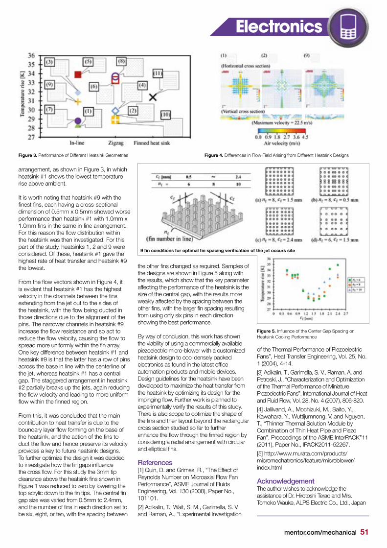
mentor.com/mechanical 51
arrangement, as shown in Figure 3, in which heatsink #1 shows the lowest temperature rise above ambient.
It is worth noting that heatsink #9 with the finest fins, each having a cross-sectional dimension of 0.5mm x 0.5mm showed worse performance than heatsink #1 with 1.0mm x 1.0mm fins in the same in-line arrangement. For this reason the flow distribution within the heatsink was then investigated. For this part of the study, heatsinks 1, 2 and 9 were considered. Of these, heatsink #1 gave the highest rate of heat transfer and heatsink #9 the lowest.
From the flow vectors shown in Figure 4, it is evident that heatsink #1 has the highest velocity in the channels between the fins extending from the jet out to the sides of the heatsink, with the flow being ducted in those directions due to the alignment of the pins. The narrower channels in heatsink #9 increase the flow resistance and so act to reduce the flow velocity, causing the flow to spread more uniformly within the fin array. One key difference between heatsink #1 and heatsink #9 is that the latter has a row of pins across the base in line with the centerline of the jet, whereas heatsink #1 has a central gap. The staggered arrangement in heatsink #2 partially breaks up the jets, again reducing the flow velocity and leading to more uniform flow within the finned region.
From this, it was concluded that the main contribution to heat transfer is due to the boundary layer flow forming on the base of the heatsink, and the action of the fins to duct the flow and hence preserve its velocity provides a key to future heatsink designs. To further optimize the design it was decided to investigate how the fin gaps influence the cross flow. For this study the 3mm tip clearance above the heatsink fins shown in Figure 1 was reduced to zero by lowering the top acrylic down to the fin tips. The central fin gap size was varied from 0.5mm to 2.4mm, and the number of fins in each direction set to be six, eight, or ten, with the spacing between
the other fins changed as required. Samples of the designs are shown in Figure 5 along with the results, which show that the key parameter affecting the performance of the heatsink is the size of the central gap, with the results more weakly affected by the spacing between the other fins, with the larger fin spacing resulting from using only six pins in each direction showing the best performance.
By way of conclusion, this work has shown the viability of using a commercially available piezoelectric micro-blower with a customized heatsink design to cool densely packed electronics as found in the latest office automation products and mobile devices. Design guidelines for the heatsink have been developed to maximize the heat transfer from the heatsink by optimizing its design for the impinging flow. Further work is planned to experimentally verify the results of this study. There is also scope to optimize the shape of the fins and their layout beyond the rectangular cross section studied so far to further enhance the flow through the finned region by considering a radial arrangement with circular and elliptical fins.
References[1] Quin, D. and Grimes, R., “The Effect of Reynolds Number on Microaxial Flow Fan Performance”, ASME Journal of Fluids Engineering, Vol. 130 (2008), Paper No., 101101.
[2] Acikalin, T., Wait, S. M., Garimella, S. V. and Raman, A., “Experimental Investigation
of the Thermal Performance of Piezoelectric Fans”, Heat Transfer Engineering, Vol. 25, No. 1 (2004), 4-14.
[3] Acikalin, T., Garimella, S. V., Raman, A. and Petroski, J., “Characterization and Optimization of the Thermal Performance of Miniature Piezoelectric Fans”, International Journal of Heat and Fluid Flow, Vol. 28, No. 4 (2007), 806-820.
[4] Jalilvand, A., Mochizuki, M., Saito, Y., Kawahara, Y., Wuttijumnong, V. and Nguyen, T., “Thinner Thermal Solution Module by Combination of Thin Heat Pipe and Piezo Fan”, Proceedings of the ASME InterPACK’’11 (2011), Paper No., IPACK2011-52267.
[5] http://www.murata.com/products/micromechatronics/feature/microblower/index.html
AcknowledgementThe author wishes to acknowledge the assistance of Dr. Hirotoshi Terao and Mrs. Tomoko Wauke, ALPS Electric Co., Ltd., Japan
9 fin conditions for optimal fin spacing verification of the jet occurs site
Figure 5. Influence of the Center Gap Spacing on Heatsink Cooling Performance
Figure 4. Differences in Flow Field Arising from Different Heatsink DesignsFigure 3. Performance of Different Heatsink Geometries
Electronics

52 mentor.com/mechanical
FloEFD™ Shines a Light on Automotive LightingBy Chris Watson, Andrey Ivanov, and Svetlana Shtilkind, Mentor Graphics
entor Graphics was approached several years ago by a leading automotive lighting
supplier to help them find a better way of numerically simulating their headlights. Like most automotive suppliers and OEMs they already had existing commercial CFD tools which they had been attempting to use in their engineering process. However, the time and effort involved in conducting these analyses needed to be reduced. The biggest bottlenecks in the process were related to handling the complex geometries inherent in headlights and in turn creating a computational
M
Condensation and Radiation Modeling Technologies in Automotive CFD Simulation
mesh of those geometries that could be effectively analyzed. Of course the source of the geometry for one of these headlights is a CAD model, and an assembly defining one of these models can be comprised of scores of parts, including many sweeping, stylized components that are used in modern lights. The intersections of all of these parts can create complex geometrical conditions that are often quite challenging to mesh with traditional approaches.
FloEFD, Mentor Graphics’ general purpose CFD software, has several key strengths that aggressively address the difficult, time
consuming aspects of preparing a headlight model for analysis that make it attractive. The first benefit is that the users can work directly on the native CAD model in their CAD tool. This eliminates the step of transferring a neutral file format model to the analysis tool, followed by the typical need to clean up any translation errors due to this process. Next, the benefit of the immersed boundary style of meshing used by FloEFD also impacts the geometry preparation. Because of this mesher the laborious step of simplifying and de-featuring the model can be greatly reduced. Geometric conditions that give other meshers difficulties, like interfering parts, small gaps and sharply pointed objects are handled by the FloEFD mesher
Figure 1. CAD model to final mesh
CAD Model = Analysis model simulation inputs applied directly to CAD modle
Rapid meshing of complex geometry, fluid+solids (including handling interfering parts)

mentor.com/mechanical 53
Automotive
Figure 2. Assembly and relevant parts
Figure 3. Film thickness development at different points in time

54 mentor.com/mechanical
and solver. The net effect is a tool that can efficiently and quickly overcome the most user-intensive, time consuming hurdle of conducting these types of analyses.
So the automotive lighting supplier began adopting FloEFD to tackle these problems. Since the main bottleneck in their process had been addressed by FloEFD, as can be human nature after a relatively brief “honeymoon” period, these strengths became accepted as the “new norm” and the attention shifted to adding advanced functionality to address the demands of a complete headlight analysis. The Mentor Graphics FloEFD development team worked closely with the customer to understand their requirements, and in each of the successive releases of FloEFD enhancements were added to help make it a complete, expert tool to tackle automotive lighting applications. Many of these enhancements focused on advanced radiation capabilities, like spectral dependencies for radiative properties, like absorptivity and emissivity (implemented in a sophisticated ray-based approach), reflectivity options like diffuse, spectral, and Gaussian reflection, and improved handling of focusing and refraction for cases in which optical effects are important as well as thermal effects in semi-transparent solids. A module to FloEFD was introduced that included these enhancements as well providing the ability to create LED compact models, in which thermal and optical data from Mentor Graphics’ T3ster ® and TeraLED® devices could be used to create a more accurate representation of an LED in a CFD model. The LED compact model is unique in that the user simply assigns the forward current to the device (rather than the typical input of heat generation rate, which may not be clearly defined) and the output from the analysis will include the junction temperature of the LED, its resulting heat power, and the luminous flux.
Another capability added to FloEFD to address an area of concern for headlight designers is the ability to simulate condensation. As newer headlight designs have incorporated lighting sources that generate less heat (in particular LEDs), condensation on the lenses of headlights can become a bigger issue. FloEFD’s water film evolution capability is able to model condensation, evaporation, and phase change (allowing for icing predictions), and display this information in a variety of quantitative and qualitative means.
Headlight ExampleThe following example highlights FloEFD’s capabilities in simulating headlights, with a particular focus on surface condensation modeling. Figure 2 displays the model and the relevant parts that were included in the simulation.
The full conjugate heat transfer problem is modeled, including convection, conduction, and radiation. Appropriate material and radiative properties are assigned to each of the parts, including the lenses being modeled as semi-transparent to radiation with a specular dependency. The air space within the headlamp assembly is modeled. Transient heat transfer boundary conditions on the external faces of the assembly are used in this example, although the external air domain could have been included as part of the analysis as well. The pressure and temperature of the air within the assembly are initialized to 101325 Pa and 25°C respectively, the initial external temperature is set to -10°C, and the relative humidity is set to 95%. The inside surface of the front lens is set as “wettable” and is the region of interest to determine whether condensation occurs. The simulation scenario being modeled is:
1. A vehicle stopped in a cold humid environment: condensation starts;
2. After 750 seconds the LEDs are switched on; and
3. After 20 minutes (1200 seconds) the engine and lights are switched on: melting starts.
As the simulation begins the solid components start to cool due to the cold external temperature. Since the air within the headlamp is initialized with a high relative humidity, condensation begins to form on the inside surface of the front lens. Figure 3 shows the progression of the film thickness of the condensation at different points in time. At 1200 seconds the halogen bulbs, as well as the engine, are turned on. This starts to add heat to the system, and it is seen from these images that the film begins to be cleared, especially in the region in front of the high beam reflector.
Figure 4. Development of film mass and temperature over time
Figure 5. Transient history of film phase
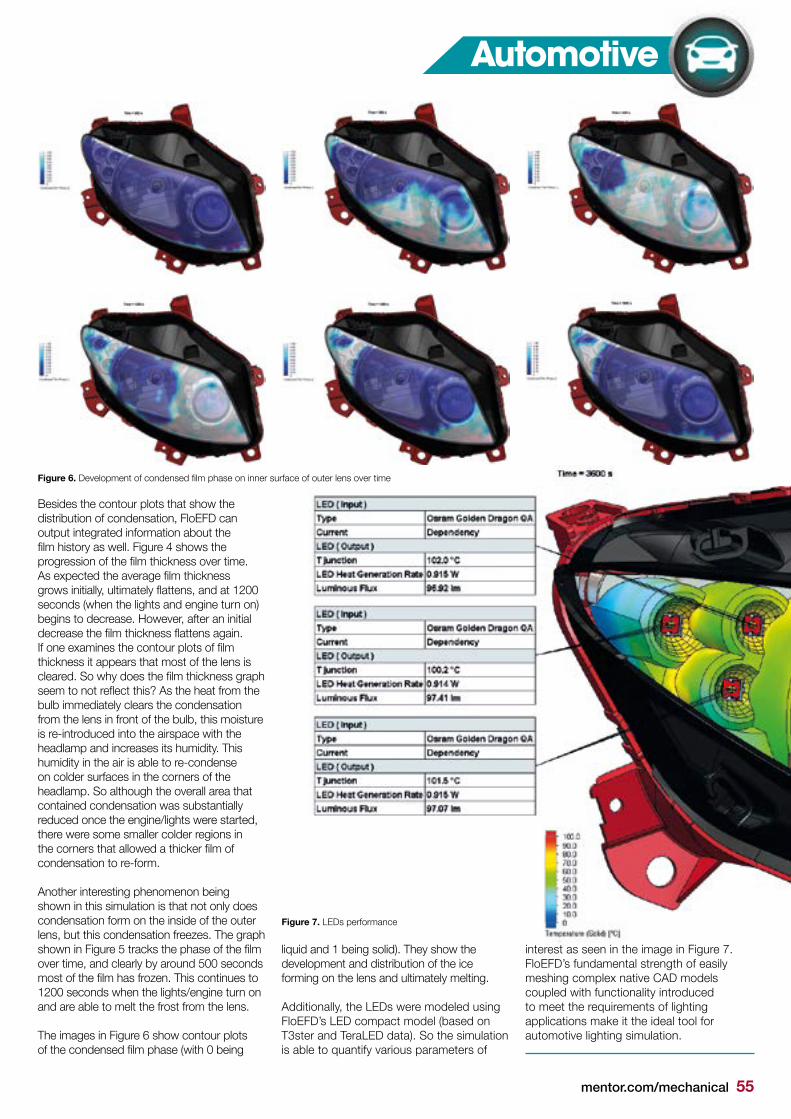
mentor.com/mechanical 55
Besides the contour plots that show the distribution of condensation, FloEFD can output integrated information about the film history as well. Figure 4 shows the progression of the film thickness over time. As expected the average film thickness grows initially, ultimately flattens, and at 1200 seconds (when the lights and engine turn on) begins to decrease. However, after an initial decrease the film thickness flattens again. If one examines the contour plots of film thickness it appears that most of the lens is cleared. So why does the film thickness graph seem to not reflect this? As the heat from the bulb immediately clears the condensation from the lens in front of the bulb, this moisture is re-introduced into the airspace with the headlamp and increases its humidity. This humidity in the air is able to re-condense on colder surfaces in the corners of the headlamp. So although the overall area that contained condensation was substantially reduced once the engine/lights were started, there were some smaller colder regions in the corners that allowed a thicker film of condensation to re-form.
Another interesting phenomenon being shown in this simulation is that not only does condensation form on the inside of the outer lens, but this condensation freezes. The graph shown in Figure 5 tracks the phase of the film over time, and clearly by around 500 seconds most of the film has frozen. This continues to 1200 seconds when the lights/engine turn on and are able to melt the frost from the lens.
The images in Figure 6 show contour plots of the condensed film phase (with 0 being
Automotive
liquid and 1 being solid). They show the development and distribution of the ice forming on the lens and ultimately melting.
Additionally, the LEDs were modeled using FloEFD’s LED compact model (based on T3ster and TeraLED data). So the simulation is able to quantify various parameters of
interest as seen in the image in Figure 7.FloEFD’s fundamental strength of easily meshing complex native CAD models coupled with functionality introduced to meet the requirements of lighting applications make it the ideal tool for automotive lighting simulation.
Figure 6. Development of condensed film phase on inner surface of outer lens over time
Figure 7. LEDs performance

Vehicle Thermal Management for
the Mitsubishi Outlander PHEVBy Atsushi Itoh, Thermal & Fluid Dynamics Engineering Development,
Vehicle Function Testing Dept., Development Engineering Office, Research & Development Center, Mitsubishi Motors Corporation, Aichi, Japan
itsubishi Motors Corporation, in Japan, today manufactures and supplies one of the most
successful and popular Plug-in Hybrid Electric Vehicles (PHEV) in the world, the Outlander Sports Utility Vehicle (SUV). Many years of R&D and cutting-edge innovation have gone into Mitsubishi’s full range of ECO vehicles and the Outlander has been a technology pioneer in its field.
To ensure the Outlander has an extended range over differing climates, and to balance the many thermal challenges in its complex design, is a major task. The Thermal & Fluids Technology Department at Mitsubishi own this task and use a wide range of Computer-Aided Engineering (CAE) tools including 3D Computational Fluid Dynamics (CFD) and 1D thermo-fluid system simulation. 1D CFD design is led by Mentor Graphics’ Flowmaster systems simulation software and is used to define all internal thermal ventilation systems for optimal performance in the Outlander.
M
Automotive
mentor.com/mechanical 57
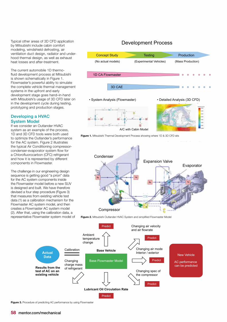
58 mentor.com/mechanical
Calibration
Base Flowmaster Model
Base Vehicle
Lubricant Oil Circulation Rate
Predict
Predict
Predict
Predict
Predict
New Vehicle
AC performance can be predicted
Changing air velocityand air flowrate
Changing air modeInterior / exterior
Changing spec of the compressor
Changing charge massof refrigerant
Ambient temperature change
ActualData
Results from thetest of AC on anexisting vehicle
Typical other areas of 3D CFD application by Mitsubishi include cabin comfort modeling, windshield defrosting, air ventilation duct design, radiator and under-hood thermal design, as well as exhaust heat losses and after-treatment.
The current automobile 1D thermo-fluid development process at Mitsubishi is shown schematically in Figure 1. Flowmaster’s powerful ability to simulate the complete vehicle thermal management systems in the upfront and early development stage goes hand–in-hand with Mitsubishi’s usage of 3D CFD later on in the development cycle during testing, prototyping and production stages.
Developing a HVAC System ModelIf we consider an Outlander HVAC system as an example of the process, 1D and 3D CFD tools were both used to optimize the Outlander’s performance for the AC system. Figure 2 illustrates the typical Air Conditioning compressor-condenser-evaporator system flow for a Chlorofluorocarbon (CFC) refrigerant and how it is represented by different components in Flowmaster.
The challenge in our engineering design sequence is getting good “a priori” data for the AC system components inside the Flowmaster model before a new SUV is designed and built. We have therefore devised a four step procedure (Figure 3) that measures from existing vehicle test data (1) as a calibration mechanism for the Flowmaster AC system model, and then creates a Flowmaster AC system model (2). After that, using the calibration data, a representative Flowmaster system model of
Figure 1. Mitsubishi Thermal Development Process showing where 1D & 3D CFD sits
Figure 2. Mitsubishi Outlander HVAC System and simplified Flowmaster Model
Figure 3. Procedure of predicting AC performance by using Flowmaster
Development Process
Concept Study Testing Production
(No actual models) (Experimental Vehicles) (Mass Production)
1D CA Flowmaster
3D CAE
A/C with Cabin Model
• System Analysis (Flowmaster) • Detailed Analysis (3D CFD)
Condenser
Compressor
Expansion ValveEvaporator

mentor.com/mechanical 59
BoundaryCondition
Compressor
Evaporator Evaporator
ExpansionValve
ExpansionValve
Rear Cooler Unit
HVACPiping
Condenser
BoundaryCondition
Figure 5. Details of Flowmaster Heat Exchanger Calibration – Step 3
Evaporator (Heat Exchanger) Flowmaster 1D Model
Refrigerant Outlet
Refrigerant Inlet
Air
Modeling Refrigerant Inlet
Air
Refrigerant Outlet
Does not match with the actualmeasurement due to phase changephenomena needing to be captured
Correction factor (k’) of the items below aredecided to match the actual measurement.
Adjustment
Heat Exchanger- Heat transfer coefficient of air side- Pressure loss of air side- Heat transfer coefficient of refrigerant side- Pressure loss of refrigerant side
the new car design is made (3). This in turn starts to change operating parameters (4) in the Flowmaster simulation to look at a range of operating ambient temperatures and assorted component operating variables as well as CFC refrigerant flow rates.
• Step 1: Measuring test data from base vehicle
• Step 2: Creating a Flowmaster AC system model
• Step 3: Calibrating with test data
• Step 4: Predicting an AC performance at a range of operating conditions
During Step 1, we utilize stand-alone AC performance data such as the compressor efficiency, heat exchange rates in the condenser and the evaporator, and any pressure drop data we may have. This step is based on an AC unit from a similar range of car using actual data such as, refrigerant temperature at the heat exchanger inlet and outlet, plus pressure measurements etc.
For Step 2, we created a Flowmaster AC system model. Figure 4 illustrates Flowmaster AC system model that represents the dual AC systems consisting of HVAC and rear cooler unit.
In Step 3, Figure 5 illustrates how we used actual measurements data to put correction factors into the Flowmaster heat exchanger models that pulled the predictions closer to reality.
In Step 4 (Figure 6), we changed specifications inside Flowmaster by
Figure 4. Details of Flowmaster Refrigerant Cycle Model (dual AC) - Step 2
Figure 6. Method of Obtaining Heat Exchanger Correction Factors for Flowmaster Model (example of changing condenser’s characteristics based on performance curve) – Step 4
Automotive

60 mentor.com/mechanical
Aver
age
Tem
pera
ture
of C
abin
[deg
C]
Time [min]
0 50 100 150 200
Test
Calculation
Model: OutlanderCondition: High temperature and high humidity
adjusting the correction coefficient, ‘k’, of the condenser based on actual operating characteristics in the SUV. The net effect, as shown in Figure 7, is that we could extrapolate with confidence into new SUV driving conditions our Flowmaster 1D thermo-fluid refrigeration system model based on the previous simulations and test data we already had. We can also incorporate the Car Cabin model component inside Flowmaster (Figure 8) in our study in order to be even closer to “real world” cabin thermal driving conditions in our systems model. Our simulation results for this approach on the Outlander PHEV are shown (Figure 9) for a particular drive cycle involving high temperature and high humidity atmospheric conditions. They show a very good synergy with subsequent test measurements, giving us confidence in our approach.
Using the Calibrated SUV Flowmaster Model for AC Compressor Load StudiesOnce we had our calibrated SUV 1D thermo-fluid AC system simulation model inside Flowmaster we can start to ask some very interesting questions. For the situation in Figure 10 where we wanted to look at a larger condenser we could run through Flowmaster a set of “what if…” variants (Table 1) and look at car speeds ranging from idling to high speed and see their potential impact on the vehicle. We can even look at a brand new vehicle (Figure 11) for the given drive cycle. This approach gives us a very powerful upfront design capability available to use for our design process.
Figure 9. Flowmaster HVAC and Car Cabin Model Predictions for a Typical Car Drive Cycle
Figure 8. Flowmaster HVAC Model with the Cabin Model Included
Pipe HVAC system
Condenser
Boundarycondition
Boundarycondition
Duct
Car Cabin
Expansion valve
EvaporatorCompressor
Heat balancemodel Car Cabin Transmission
Convection
Thermalconduction
Reflection
Figure 7. Thermal Prediction Results for a Range of SUV Driving Conditions Versus Actual Data using this Calibrated Flowmaster Approach – Steps 1 to 4 (Extrapolation to New Conditions)
Evaporator exit airtemperature (°C)
Predict
Base Model Range of Driving conditions
ActualData
Results after testingan existing A/C
Adjust FlowmasterBase Model
Changing ambienttemperature
Steps 2 and 3
Steps 4
Steps 15°C
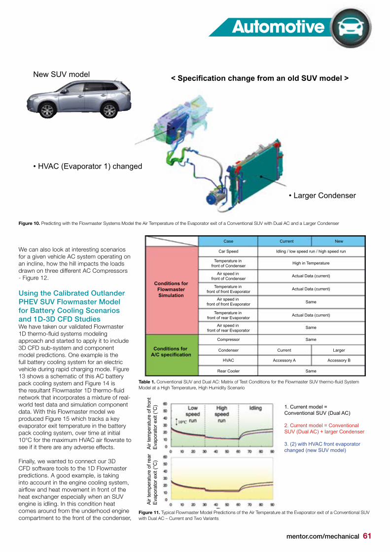
mentor.com/mechanical 61
New SUV model
• HVAC (Evaporator 1) changed
• Larger Condenser
< Specification change from an old SUV model >
Table 1. Conventional SUV and Dual AC: Matrix of Test Conditions for the Flowmaster SUV thermo-fluid System Model at a High Temperature, High Humidity Scenario
Figure 11. Typical Flowmaster Model Predictions of the Air Temperature at the Evaporator exit of a Conventional SUV with Dual AC – Current and Two Variants
Automotive
Conditions forFlowmasterSimulation
Conditions for A/C specification
Case Current
Car Speed
Compressor
Condenser
HVAC
Rear Cooler
Idling / low speed run / high speed run
High in Temperature
Actual Data (current)
Actual Data (current)
Temperature in front of Condenser
Air speed in front of Condenser
Temperature in front of front Evaporator
Air speed in front of front Evaporator
Temperature in front of rear Evaporator
Air speed in front of rear Evaporator
Actual Data (current)
Same
Same
Same
Same
New
Current Larger
Accessory A Accessory B
Air t
empe
ratu
re o
f fro
ntEv
apor
ator
exi
t (°C
)Ai
r tem
pera
ture
of r
ear
Evap
orat
or e
xit (
°C)
Time
1. Current model =Conventional SUV (Dual AC)
2. Current model = ConventionalSUV (Dual AC) + larger Condenser
3. (2) with HVAC front evaporatorchanged (new SUV model)
Figure 10. Predicting with the Flowmaster Systems Model the Air Temperature of the Evaporator exit of a Conventional SUV with Dual AC and a Larger Condenser
We can also look at interesting scenarios for a given vehicle AC system operating on an incline, how the hill impacts the loads drawn on three different AC Compressors - Figure 12.
Using the Calibrated Outlander PHEV SUV Flowmaster Model for Battery Cooling Scenarios and 1D-3D CFD StudiesWe have taken our validated Flowmaster 1D thermo-fluid systems modeling approach and started to apply it to include 3D CFD sub-system and component model predictions. One example is the full battery cooling system for an electric vehicle during rapid charging mode. Figure 13 shows a schematic of this AC battery pack cooling system and Figure 14 is the resultant Flowmaster 1D thermo-fluid network that incorporates a mixture of real-world test data and simulation component data. With this Flowmaster model we produced Figure 15 which tracks a key evaporator exit temperature in the battery pack cooling system, over time at initial 10°C for the maximum HVAC air flowrate to see if it there are any adverse effects.
Finally, we wanted to connect our 3D CFD software tools to the 1D Flowmaster predictions. A good example, is taking into account in the engine cooling system, airflow and heat movement in front of the heat exchanger especially when an SUV engine is idling. In this condition heat comes around from the underhood engine compartment to the front of the condenser,

62 mentor.com/mechanical
Electriccompressor
Blower
Battery cooling system image
Electromagnetic valve
HVAC
Expansion valve Driving battery cooling evaporator
Battery pack
EA ra
diat
or
A/C
Con
dens
er
Engi
ne R
adia
tor
Oil
Cool
er
Radi
ator
Fan
Condenser
HVAC
Compressor
Duct
Car Cabin
Battery Pack
BatteryEvaporator
Figure 14. Flowmaster Battery Cooling System Model of a Mitsubishi Outlander PHEV Figure 15. Predicted Flowmaster Mitsubishi Outlander PHEV Evaporator Temperature during Rapid Charging
Air
tem
pera
ture
beh
ind
evap
orat
or [°
c]
0 500 1000 1500 2000 2500
Time [s]
Figure 12. Flowmaster 1D AC System Model Predictions for Compressor Load Performances of an SUV going up an Incline for three possible Compressor Types
Figure 13. Schematic Battery Cooling System of a Mitsubishi Outlander PHEV
Engine power 10PS(low revolution up an incline)
Hill-climbingresistance
Base Car New Car
Compressor load(max refrigerated airconditioning)
(Note: 1PS = 0.986 HP)
2~3PS • Air conditioning component carry-over• Shifting to dual air conditioning
Compressor 1
Compressor 2
Compressor 3
LoadLarge Smaller
TemperatureHigh Low
0 500 1000 1500 2000 2500
Com
pres
sor L
oad
P [k
w]
Engine Speed Ne (rpm)0 1000 1500 2000 2500
Air
Tem
pera
ture
of
Eva
pora
tor e
xit
[deg
C]
Compressor Speed Nc [rpm]

mentor.com/mechanical 63
1D CFD 3D CFD
The temperature infront of condenserwhen idling isobtained via 3D CFDanalysis
When running When idling
Before AfterCase
Car speed Idling (Compressor 1000rpm)
Use result of 3D CFD analysis
Use result of 3D CFD analysis
Same
Same
Same
Same
Base Modified
Temperature in front of condenser
Air speed in front of condenser
Temperature in front of evaporator
Air speed in front of evaporator
Compressor
Condenser
HVAC
Conditions forFlowmasterSimulation
Conditions forspecification
Before
(DesignModifications)
After
(DesignModifications)
3D CFD
After
Before
Surrounded by heatNo = Heat recirculation Yes = idling
0.5 MPa
Surrounded by heatNo = Heat recirculation Yes = idling
DesignIteration:
#1 #2 #3 #4
Hea
t exc
hang
e ra
te o
f con
dens
erA
ir te
mpe
ratu
re o
f eva
pora
tor e
xit
Dis
char
ge p
ress
ure
of c
ompr
esso
r
0.5kW
1°C
Before
After
Before
After
leading to a rise in temperature (Figure 16). We found we could calculate ambient air temperatures in front of the condenser by doing a series of 1D and 3D CFD calculations alternately until an equilibrium value was obtained. This allowed us to take into account the fan at the back of the condenser and the recirculating air in the engine from the 3D CFD within the 1D CFD systems simulations, and yielding a more accurate prediction than either would give separately. We could also produce a set of loosely coupled simulations for a wide range of compressor conditions as shown in Table 2 for a given high temperature, high humidity driving scenario. With the combined 1D-3D CFD approach we were able to look at a new design modification inside the engine compartment within the 3D CFD model and see its desired impact in the 1D model for idling and non-idling driving conditions. Figure 17 which shows that we have had a beneficial impact after the design modification.
To summarize, we have outlined how we pre-consider air-conditioning systems for Mitsubishi vehicles using Flowmaster’s simple AC model for calculating cooling performance to support our vehicle developments over short timescales and in a flexible way. Currently, our 1D and 3D co-operative analysis approach is leading our accuracy improvements. We use it to evaluate equipment parts and it is ideal to have the performance of each single, required AC part, simulated to satisfy the targeted cooling system performance level. For this reason, Mitsubishi is looking into using this calculation method with design space optimization tools going forward.
Figure 16. 1D– 3D CFD Simulation of SUV Heat Exchanger Performance Scenarios when Running Freely and in Idling Mode
Table 2. 1D-3D CFD simulation Matrix of Test Conditions for the Flowmaster System Model of an Idling/Free Running SUV at a High Temperature, High Humidity Scenario
Figure 17. 1D– 3D CFD Simulation of SUV Heat Exchanger Performance Predictions when Running Freely and in Idling Mode for a Base Case and a Design Modification
Automotive

64 mentor.com/mechanical
Reading Between the Thermal LinesBy Hui Zhang, M.Sc., Dipl.-Phys. Max Wagner, and Prof. Dr.-Ing. habil. Tran Quoc Khanh, Laboratory of Lighting Technology, Technische Universität Darmstadt
New Dielectric Materials for LED-Packages
ne of the main aims in electronic packaging is a good heat transport away from the device, downwards
through the package into the board. The LED chip is connected electrically at its top and bottom. That is why there is a need to separate the electric circuit from the metal board. This is achieved by an insulator layer, which is neither electrically nor thermally very conductive. In this study the thermal behavior of new dielectric materials in LED packages are investigated. Furthermore the influence of geometric parameters of the electrical layout has been tested by measurements and simulations.
Figure 1 shows the structure of a high power LED based on a chip-on-board-package. The chip (also called die) not only produces light, but also a certain amount of heat, which should be as low as possible. The majority of the heat from the die will be transferred to the outside by why of conduction. Since the thermal conductivity of molding compounds (e.g. epoxy or silicone) is much smaller than that of the die attach (e.g. silver conductive adhesive), most of the heat will conduct downwards. Parameters such as the thermal conductivity and the geometrical structure of the interface materials have high influences on the heat flow. So a change would lead to different measurement results with the thermal impedance test system T3ster.
Figure 2 shows the structure function of an LED package after the evaluation of the measurement. The structure function presents all the thermal information of the tested LED-package, including
O
thermal resistance in K/W and thermal capacity in Ws/K. In fact every layer of the thermal capacity represents one kind of a material in the LED-package. The thermal resistances of different materials are of great interests to us, because the electrical components need to be cooled.
Of course a lower thermal resistance means a better performance.
Electrical LayoutConsidering the electrical connection between the chip and external electrodes, the electric layout plays a very important
Figure 1. Structure of a high power LED-package
Figure 2. Structure function of an LED-Package

mentor.com/mechanical 65
Electronics
role in an LED package. In view of the electric conductivity and cost, copper is the first choice to the manufacturers. That is why different geometrical structures of the electric layout were built and analyzed in a thermal perspective. Beside the size of the surface, the thickness of the layout has been changed in values of 35, 70 and 105 µm. Copper has a high thermal conductivity of λ=385 W/mK. For a copper layout with a surface area of 5 mm x 5 mm and a thickness of 35 µm, the thermal resistance is
This value is so small that a triplication of the thickness to 105 µm leads to only 0.01 K/W. So, why the concern over thickness? The answer lies in the effect of heat spreading, which is not represented by the formula above, but rather detected in measurement results. Figure 3 shows the approach of the effect by using a refraction model [1].
The die’s heat flow reaches the copper layer and will be spread in this material. Compared to optics the refraction at the boundary surface is dependent on the refraction index, which is the conductivity in the thermal picture. The chip’s junction to a high conductive material means a high refraction angle α, so that a high spreading effect should appear. By increasing the copper layout’s thickness, the surface A, which is flown through by the heat, gets larger. Now, we can calculate the next thermal resistance with the simple formula again. The experimental results and transient thermal simulation with FloTHERM are shown in the following figures 4 and 5.
Both results confirm that the total thermal resistance with a thicker copper layout is lower. That is because heat flows into the dielectric with a higher surface area (Figure 3). So the dielectric itself has a
smaller thermal resistance. Since a thicker thickness means more material, a higher thermal capacity should be observed. Since very thin layers mean a long simulation time, the thicknesses of glue and dielectric differ to the test devices. The trend of lower thermal resistance and higher capacity by enlarging the
copper layout’s thickness appears in measurement and simulation data.
New Dielectric MaterialsAll used dielectric are based on polymer and/or ceramic materials. The techniques to connect the dielectric layer with the board’s substrate and electrical layout
Figure 3. Heat spreading at different thicknesses of electrical layout
Figure 4. Structure functions (measurement data)
Figure 5. Simulation data (variation of the thickness)

66 mentor.com/mechanical
differ. A standard method, is laminating the electrical layout on a ceramic filled polymer by an epoxy adhesive. Since the thermal conductivity of polymer is lower than that of ceramic, a new approach is to use a ceramic layer that consists of nano-crystalline aluminum oxide crystals (Al2O3) [2]. The electrical layout is laminated on this pure ceramic layer, or even contacted directly by a metallization process. Samples with the same LED package, but different dielectrics are tested with the thermal impedance measurement. A direct comparison of Nanotherm LC and a ceramic paste (Figure 6) as well as Nanotherm DM and a ceramic filled polymer has been made. Figures 8 and 9 show the results of the measurement’s structure functions.
Thermal resistances of dielectric and substrate build the main part of the total thermal resistance in the investigated LED-package. The use of a laminated nano-ceramic instead of a ceramic paste reduces the thermal resistance from 40 to 10 K/W (Figure 8). One reason for this is the small thickness of the ceramic layer (10 µm). The direct comparison of pure nano-ceramic with a laminated ceramic filled polymer of a standard PCB also shows a reduction of the dielectric’s thermal resistance of about 33%.The conductivity is higher and the thickness of the direct metallized material is smaller, so the consequence must be a reduction in the total thermal resistance.
ConclusionNot every transient behavior can be covered by a simple one-dimensional calculation. Heat spreading effects in
Figure 6. Comparison of Nanotherm LC (Laminated Circuit) and ceramic paste [3]
Figure 9. Structure functions of Nanotherm DM
Figure 7. Comparison of Nanotherm DM (Direct metallization) and ceramic filled polymer [3]
Figure 8. Structure functions of Nanotherm LC and a ceramic paste as dielectric material
the electrical layout directly affect the measurement curves and must be considered by other models. The change of the PCB’s dielectric has the biggest effect on the total thermal resistance. Beside a standard ceramic filled polymer, new dielectric materials are tested. A direct comparison of laminated and direct metallized Nanotherm, and the aging behavior and reliability of both materials are interesting aspects that should be studied in the future.
References:[1] David P. Kennedy. “Heat conduction in a homogeneous solid circular cylinder of isotropic media”. Product Development Laboratory, Data Systems Div., International Business Machines Corp, Poughkeepsie, NY, 1959.
[2] http://www.camnano.com
[3] Data sheet from Excelitas Technologies and Cambridge Nanotherm.

mentor.com/mechanical 67
Power Generation
familiar dilemma for any instrumentation engineer… you need to measure a system fluid property accurately but
the very presence of instrumentation in the system affects the property that you are trying measure. This is nowhere better illustrated than in the case of pressure measurement in small bore pipework, where nothing less than a rigorous approach to instrumentation design will have a significant impact on measurement accuracy.
An ongoing collaborative Mechanical Analysis Division research program, aimed at providing validation data for the Flowmaster 1D thermo-fluid simulation tool recently faced exactly this challenge. The rig comprised a number of component types normally associated with a vapor cycle system, all linked together by extensive copper pipework of 22mm outside diameter (c. 7/8”) and of a nominal bore of 20mm. The test plan required that pressure (P) and temperature (T) were measured before and after every major component, so that a precise profile of pressure drop and temperature change throughout the system could be constructed. This meant the design and manufacture of 14 pairs of P&T tappings to facilitate the connection of remotely mounted pressure transducers and the insertion of 1.5mm diameter Type K thermocouple probes. From the outset it was recognized that in order to achieve minimum flow disturbance the tapping assemblies should be sited in straight lengths of pipework, i.e. away from bends and junctions, and with the thermocouple positioned downstream of the pressure tapping. The resulting solution was designed for ease of manufacture and employed two standard reduced-branch tees,
FloEFD™ Improves the Accuracy of Validation Rig Measurements
A
Figure 2. End view of ‘reduced branch’ copper Tee
Figure 1. Initial concept for pressure and temperature measurement tappings
By Steve Streater, Senior Product Manager;and Richard Merrett, Engineering Intern, Mechanical Analysis Division, Mentor Graphics
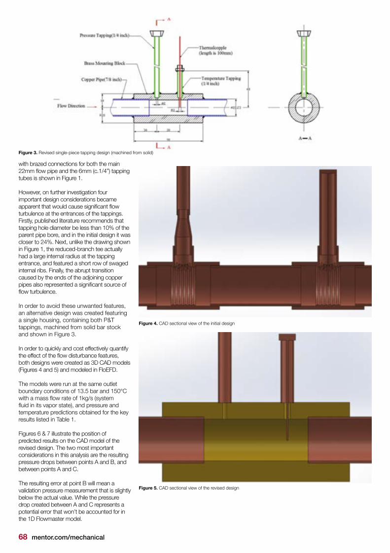
68 mentor.com/mechanical
with brazed connections for both the main 22mm flow pipe and the 6mm (c.1/4”) tapping tubes is shown in Figure 1.
However, on further investigation four important design considerations became apparent that would cause significant flow turbulence at the entrances of the tappings. Firstly, published literature recommends that tapping hole diameter be less than 10% of the parent pipe bore, and in the initial design it was closer to 24%. Next, unlike the drawing shown in Figure 1, the reduced-branch tee actually had a large internal radius at the tapping entrance, and featured a short row of swaged internal ribs. Finally, the abrupt transition caused by the ends of the adjoining copper pipes also represented a significant source of flow turbulence.
In order to avoid these unwanted features, an alternative design was created featuring a single housing, containing both P&T tappings, machined from solid bar stock and shown in Figure 3. In order to quickly and cost effectively quantify the effect of the flow disturbance features, both designs were created as 3D CAD models (Figures 4 and 5) and modeled in FloEFD. The models were run at the same outlet boundary conditions of 13.5 bar and 150°C with a mass flow rate of 1kg/s (system fluid in its vapor state), and pressure and temperature predictions obtained for the key results listed in Table 1.
Figures 6 & 7 illustrate the position of predicted results on the CAD model of the revised design. The two most important considerations in this analysis are the resulting pressure drops between points A and B, and between points A and C.
The resulting error at point B will mean a validation pressure measurement that is slightly below the actual value. While the pressure drop created between A and C represents a potential error that won’t be accounted for in the 1D Flowmaster model.
Figure 4. CAD sectional view of the initial design
Figure 3. Revised single-piece tapping design (machined from solid)
Figure 5. CAD sectional view of the revised design
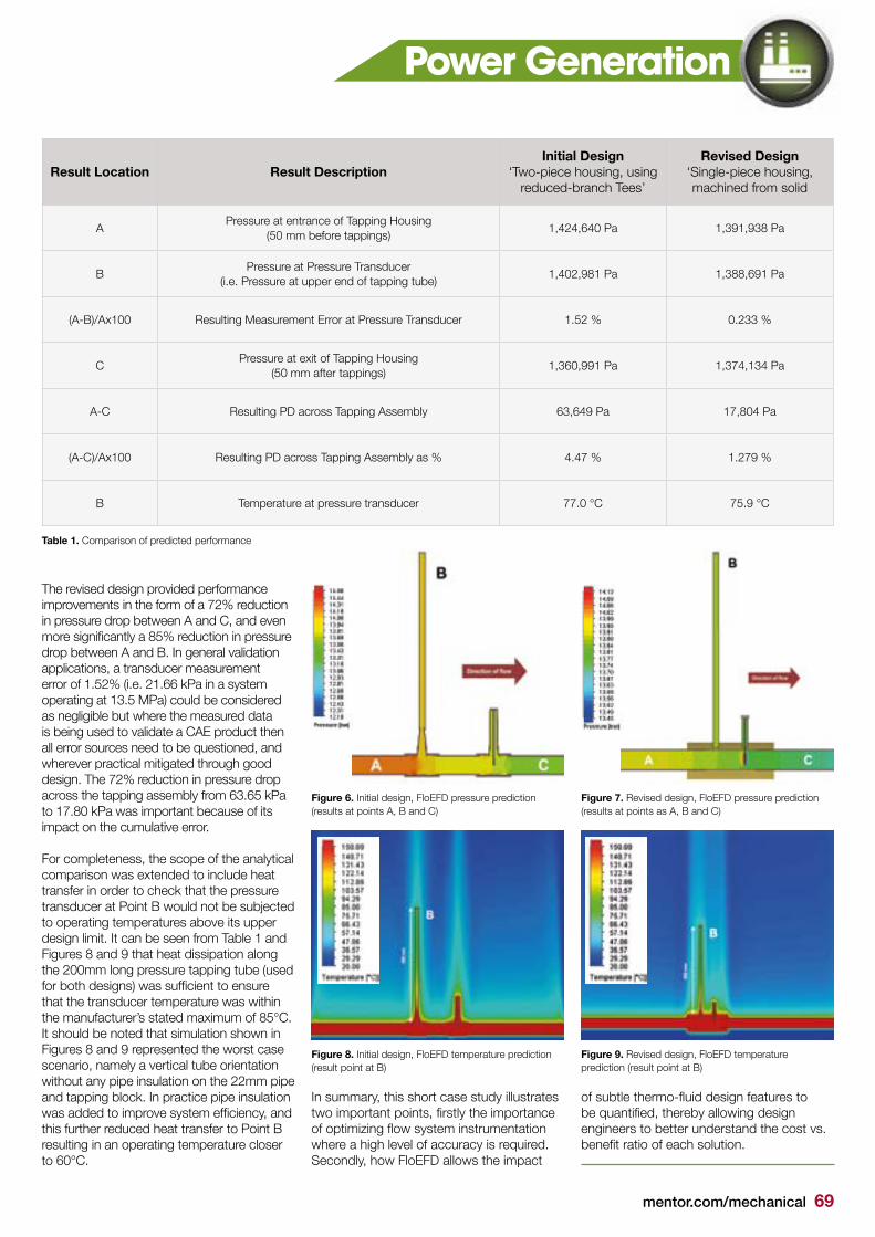
mentor.com/mechanical 69
Power Generation
The revised design provided performance improvements in the form of a 72% reduction in pressure drop between A and C, and even more significantly a 85% reduction in pressure drop between A and B. In general validation applications, a transducer measurement error of 1.52% (i.e. 21.66 kPa in a system operating at 13.5 MPa) could be considered as negligible but where the measured data is being used to validate a CAE product then all error sources need to be questioned, and wherever practical mitigated through good design. The 72% reduction in pressure drop across the tapping assembly from 63.65 kPa to 17.80 kPa was important because of its impact on the cumulative error.
For completeness, the scope of the analytical comparison was extended to include heat transfer in order to check that the pressure transducer at Point B would not be subjected to operating temperatures above its upper design limit. It can be seen from Table 1 and Figures 8 and 9 that heat dissipation along the 200mm long pressure tapping tube (used for both designs) was sufficient to ensure that the transducer temperature was within the manufacturer’s stated maximum of 85°C. It should be noted that simulation shown in Figures 8 and 9 represented the worst case scenario, namely a vertical tube orientation without any pipe insulation on the 22mm pipe and tapping block. In practice pipe insulation was added to improve system efficiency, and this further reduced heat transfer to Point B resulting in an operating temperature closer to 60°C.
Result Location Result DescriptionInitial Design
‘Two-piece housing, using reduced-branch Tees’
Revised Design‘Single-piece housing, machined from solid
APressure at entrance of Tapping Housing
(50 mm before tappings)1,424,640 Pa 1,391,938 Pa
BPressure at Pressure Transducer
(i.e. Pressure at upper end of tapping tube)1,402,981 Pa 1,388,691 Pa
(A-B)/Ax100 Resulting Measurement Error at Pressure Transducer 1.52 % 0.233 %
CPressure at exit of Tapping Housing
(50 mm after tappings)1,360,991 Pa 1,374,134 Pa
A-C Resulting PD across Tapping Assembly 63,649 Pa 17,804 Pa
(A-C)/Ax100 Resulting PD across Tapping Assembly as % 4.47 % 1.279 %
B Temperature at pressure transducer 77.0 °C 75.9 °C
Table 1. Comparison of predicted performance
In summary, this short case study illustrates two important points, firstly the importance of optimizing flow system instrumentation where a high level of accuracy is required. Secondly, how FloEFD allows the impact
of subtle thermo-fluid design features to be quantified, thereby allowing design engineers to better understand the cost vs. benefit ratio of each solution.
Figure 7. Revised design, FloEFD pressure prediction (results at points as A, B and C)
Figure 9. Revised design, FloEFD temperature prediction (result point at B)
Figure 6. Initial design, FloEFD pressure prediction (results at points A, B and C)
Figure 8. Initial design, FloEFD temperature prediction (result point at B)

JSAE Benchmark of Automotive
Aerodynamic Test Measurements
By Boris Marovic, Automotive Industry Manager, Mentor Graphics
he Society of Automotive Engineers of Japan (JSAE) recently conducted a blind benchmark for commercial
Computational Fluid Dynamics (CFD) software to demonstrate their accuracy against test validation data on a new car shape [1]. Participants simulated a ¼-scale wind tunnel car model. The aerodynamic test model consisted of the “Ahmed” vehicle body (see Figure 1) with a full vehicle length of 1,100mm without the “additional part” at the end of the vehicle (Case 1) and at a length of 1,250mm with the additional part attached (Case 2). The height of the vehicle was 355 mm, the width 320mm, and the underfloor vertical gap was 15mm.
Each CFD software package had to analyze the airflow around the model and compare their prediction accuracies to experimental data without knowing the data beforehand. In particular, JSAE wanted to verify how accurate each CFD tool was at predicting boundary-layer separation, pressure distribution, and body forces on the model. It was up to the participants in the benchmark to choose the best meshes and turbulence models in their CFD codes to offer their best prediction.
T
Ahmed-Type Car Body Versus CFD Software Predictions
Automotive
mentor.com/mechanical 71

72 mentor.com/mechanical
Figure 1. The JSAE Aerodynamic Test Ahmed Vehicle Body with and without the additional part at the end of the vehicle
Figure 2. The model of the test chamber for the wind-tunnel experiment
Figure 3. Pressure coefficient measurement point distribution on the JSAE car body
Figure 4. Wake measurements at y/W = 0.0 for the JSAE car body: a) the case without the additional part and b) the case with the additional part
The commercial CFD participants were provided with data that included support pole shape, test section shape, and vehicle model shape plus the specification of the wind tunnel test section (Figure 2). The participants were provided with reference tunnel data as well as the specified conditions for the test. Simulations were all to be at a velocity of 25.0 m/s; the fluid properties were given as a density of 1.17 kg/m³ and a kinematic viscosity of 1.56 x 10⁻⁵ m²/s, which resulted in a Reynolds number for the test of 1.76 x 10⁶.
All CFD simulation software had to provide results for drag, lift, and pitching-moment coefficients as well as pressure coefficient at various sections of the vehicle body. Sections vertically to the car were compared to measurements at the center plane (y/W = 0.0), 12.5% off center (y/W = 0.125), and 25% off center (y/W = 0.25), where W is the width of the body. The underfloor section was only analyzed at the vertical center plane as it was not disturbed by the wind-tunnel fixture as the top side was. The section horizontal to the car was compared at 25% (z/H = 0.25) of the car height as shown in Figure 3 where 'H' is the height of the body.
The airflow wake predictions behind the car model were analyzed at the vertical lines of x = 1,000mm (line 1), x = 1,050mm (line 2), x = 1,100mm (line 3) and x = 1,200mm (line 4) – see Figure 4 - and compared to experimental measurements in the Blind Benchmark.
Seven organizations (Table 1) provided submissions to the JSAE blind benchmark (encompassing most of the main commercial CFD codes available in the market today) and they all had three months to submit their simulation results and technical information on their CFD computation approaches, physical models, and resolution scales. KKE Inc., a Mentor

mentor.com/mechanical 73
Calculation Time (h)
SoftwareComputer
CharacteristicsCores Steady State Transient
Time Step (s)
AcuSolveHP ProliantDL360p
Gen8, Xeon E5-2660 (2.2 GHz)
16No Flat Panel: 4.2 With Flat Panel:
5.9- -
ANSYSFluent R14.5
Dell PowerEdge R720 (2.9 GHz) 32 4 60 2.0 x 10⁻⁴
FloEFD HP Z600, Intel Xeon X5670 (2.93 GHz) 6 17 - -
iconCFD Intel® Xeon® Processor E5645 (2.4 GHz) 72 - No Flat Panel: 254
With Flat Panel: 267 5.0 x 10⁻⁵
PAM-FLOW HP BL460c, Intel Xeon E5-2680 (2.7 GHz) 16 40 155 5.352 x 10⁻⁵
SCRYU/Tetra (DES)
Intel Xeon E5-2690 (2.9 GHz)
48
- 33 1.0 x 10⁻⁴
SCRYU/Tetra (SAS) - 34 1.0 x 10⁻⁴
STAR-CCM+ v7.06 (IDDES)
Dell Power Edge, Intel® Xeon® CPU X5675
(3.07 GHz)120 - ~200 1.0 x 10⁻⁴
STAR-CCM+ v7.06v (SST k-ω) 12 17.5 - -
Table 2. For the participating CFD Codes in the JSAE blind automotive aerodynamic benchmark, computational resource and time required for the calculations
Graphics reseller in Japan, submitted simulation results using the CAD-embedded CFD software, FloEFD™.
Table 1 shows that the cell count was 4 to 11 times lower for FloEFD than the other CFD tools for the cases considered, it uses partial cells that can contain several sub-control volumes and a special boundary layer treatment that does not need a fine cell resolution of the boundary layer as other tools do. Also, it is worth noting that a large number of CFD calculations shown in Table 1 were conducted in transient mode, which usually results in very high CPU time for the calculation even with a high number of cores due to the large number of cells employed. More information on each code’s CFD simulation set-up can be found in the original JSAE benchmark paper [1].
ResultsFor the FloEFD simulations, KKE Inc. used the Cartesian mesh approach with solution adaptive refinement (Figure 5) on an octree basis and local meshes around the body [2-3]. Each cell level refinement was easily set-up in FloEFD and the rest of the mesh generation adaptation process was automated. The adaptive refinement can also be limited to a certain region of the domain by a maximum level being applied to the cell count so that the code does not explode the mesh size and thus helping to prevent very high CPU times. Table 2 shows the computational effort used by the seven software tools used in the blind benchmark.
Compared to the other tools, FloEFD required less resources and less calculation time to come up with good overall results, and it shows quite good agreement with the wind-tunnel experimental measurements too (Figures 6-8).
Figures 6 - 8 show the simulation prediction results for all of the CFD codes employed in the benchmark plus the error margin of the test experiment data for drag, lift, and pitching moments. The blue dashed lines show the upper and lower error margin for Case 1, without the additional part, and the red dashed lines show the margin for Case 2, with the additional part. In Figure 6, the drag coefficient (CD) of AcuSolve (Inflow 2), FloEFD, and STAR-CCM+ (IDDES) were all within the margin of error for Case 1 followed by SCRYU/Tetra (DES) with a lower value and then iconCFD again with a little lower CD. For Case 2, none of
Participants SoftwareCompressible/ Incompressible
Steady State/ Transient
Turbulence Model
JSOL Corporation AcuSolve Incompressible Incompressible Steady state Spalart Allmaras
ANSYS Japan K.K. ANSYSFluent R14.5 Incompressible Transient Scale Adaptive Simulation (SAS)
Kozo Keikaku Engineering Inc. FloEFD Compressible Steady state Modified k-Σ
Icon Technology & Process Consulting Ltd. iconCFD Incompressible Transient Spalart Allmaras
ESI Group PAM-FLOW Incompressible Transient SGS
Software Cradle SCRYU/Tetra Incompressible Transient SST-DES, SST-SAS
CD-adapco STAR-CCM+ v7.06 Compressible, Incompressible
Transient, Steady state
IDDES (SST), SST k-ω
Software Mesh Type
Number of Cell Layers in the Boundary
Layer
Number of Cells
Without Rear Flat Panel (Case 1)
Number of Cells
With Rear Flat Panel (Case 2)
Mesher Used
AcuSolve Tetrahedral mesh 7 24,755,000 25,795,000 AcuConsole1.8b
ANSYSFluent R14.5
Unstructured grid 17 16,000,000 16,700,000ANSYSMeshing R14, TGridR14
FloEFDCartesian mesh based on octree
technology- 3,520,000 FloEFD
iconCFDHexahedral
dominant mesh7 37,640,000 38,300,000 foamProMesh
PAM-FLOW Tetrahedral mesh 6 38,260,000 PAMGEN3D
SCRYU/Tetra (DES, SAS)
Tetrahedral mesh with prisms
10 27,000,000 SCRYU/Tetra
STAR-CCM+ v7.06 (IDDES,
SST k-ω)
Hexahedral dominant mesh
20 16,690,000 16,835,000 STAR-CCM+ v7.06
Table 1. Participant Companies and CFD Codes in the JSAE blind automotive aerodynamic benchmark
Automotive

74 mentor.com/mechanical
the codes were exactly within the error margin but iconCFD made it the closest, followed by STAR-CCM+ (IDDES) and then AcuSolve (Inflow 2).
In Figure 7, the same dashed lines show the error margins also for Case 1 and 2 but here the graph shows the lift coefficient (CL). For Case 1 only, FloEFD was exactly within the margin. Slightly out of margin were STAR-CCM+ (SST k-ω), SCRYU/Tetra (SAS), and AcuSolve (Inflow 1) all at the same level, followed by AcuSolve (Inflow 2) with a larger CL. For Case 2, the test margin was very narrow and none of the codes were exactly within it. STAR-CCM+ (SST k-ω) was the closest, followed by ANSYS Fluent and then AcuSolve (Inflow 1), but with larger discrepancies.
The pitching moment coefficient predictions are shown in Figure 8 where they have the same margin color notation as before. In this graph, the error margin for Case 1 is very narrow and none of the CFD codes made it exactly within the margin. The closest were STAR-CCM+ (IDDES), followed by PAM-FLOW, and then SCRYU/Tetra (SAS) and STAR-CCM+ (SST k-ω) who were equally distant but on the lower margin compared to PAM-FLOW. Case 2 has a larger margin, and only FloEFD made it inside the margin, followed by ANSYS Fluent slightly outside the lower margin line and then with a slightly lower value SCRYU/Tetra (SAS) and AcuSolve (Inflow 2), with the same distance but on opposite sides of the margin.
It can therefore be concluded from the results of the JSAE benchmark that FloEFD was very accurate for both drag and lift in Case 1 and had the best pitching moment prediction in Case 2. STAR-CCM+ also comes out very well from the exercise if an expert user chooses the right turbulence model for the particular case
Figure 5. Computational mesh used by FloEFD for the JSAE benchmark model
Figure 6. Drag coefficients for all CFD codes for Cases 1 and 2 with the experimental Test Data error margins in blue dashed lines (Case 1) and red dashed lines (Case 2)
Figure 7. Lift coefficients for all CFD codes for Cases 1 and 2 with the experimental Test Data error margins.
Figure 8. Pitching-moment coefficients for all CFD codes for Cases 1 and 2 with the experimental Test Data error margins.
Figure 9. Comparative CFD results versus experimental measurements for the pressure coefficient at the top surface of the JSAE model at y/W= 0.125 for x/L > 0.5

mentor.com/mechanical 75
Figure 11. Comparative CFD results versus experimental measurements for the pressure coefficient at the top surface of the JSAE model at y/W = 0.25 for x/L > 0.5
Figure 12. Comparative CFD results versus experimental measurements for the pressure coefficient at the top surface of the JSAE model at y/W = 0.0
Figure 13. Centerline velocity distribution test results versus CFD code predictions for JSAE Cases 1 and 2
being simulated. When looking at pressure coefficients measured on the car body surface (see Figure 3 for locations), Figures 9 through 12 show comparatively how well AcuSolve (Inflow 2), STAR-CCM+ v7.06 (SST k-ω), FloEFD, and ANSYS Fluent R14.5 matched the experimental data for the two cases being considered.
Finally, Figure 13 illustrates the experimental test results from particle imaging velocimetry (PIV) measurements as a contour plot post-processed to compare with most of the CFD simulation software predictions. FloEFD and STAR-CCM+ (SST k-ω) can be seen to most closely match the wind-tunnel experimental results the best.
ConclusionsAlthough the meshing and solver technology of FloEFD is a non-traditional CFD approach, this JSAE blind benchmark has proven that FloEFD is as accurate as, or better than, other traditional commercial CFD software in a difficult automotive external aerodynamic study. FloEFD ranks well alongside STAR-CCM+, whilst using fewer cells, a single sophisticated turbulence model, and lower CPU times to achieve the same level of results. In addition, it was worth pointing out that with FloEFD’s out-of-the-box software, it also takes less time to set-up and optimally mesh the automotive body model, in addition to activating the single transitional k-Σ turbulence model compared to the many turbulence models some of the other codes employed, that required expert interventions.
References[1] Nakashima, Takuji; Sasuga, Nobuhiro; Ito, Yuichi; Ikeda, Masami; Ueda, Iichiro; Kato, Yoshihiro; Kitayama, Masashi; Kito, Kozo; Koori, Itsuhei; Koyama, Ryutaro; Shimada, Yoshihiro; Hanaoka, Yuji; Higaki, Tatsuhiko; Fukuda, Kota; Yamamura, Jun; Li, Ye (2013). Benchmark of Aerodynamics CFD of Simplified Road Vehicle Model: JSAE. Paper Number: 20134343. Pages 8 – 28, http://bookpark.ne.jp/jsae/pdf_e.asp
[2] Advanced Immersed Boundary Cartesian Meshing Technology in FloEFD: Mentor Graphics, http://go.mentor.com/2gogl
[3] Enhanced Turbulence Modelling in FloEFD™: Mentor Graphics, http://go.mentor.com/2glzd
Figure 10. Comparative CFD results versus experimental measurements for the pressure coefficient at the top surface of the JSAE model at y/W = 0.125
Automotive

76 mentor.com/mechanical
Geek Hub
sn’t the internet a wonderful thing!? You can find pretty much anything from anywhere at any time these days. For example you can watch renowned astrophysicist Walter Lewin’s MIT
video lectures on physics [1]. One video I found recently, that piqued my interest was Ben Krasnow’s YouTube video “The Physics of Floating Screwdrivers” [2]. The video shows a screwdriver floating in the air flow generated by pressurized air using a conventional industrial air gun. There are numerous examples on the internet, like floating tennis balls or eggs. As an enthusiastic engineer, I’m always diving into the technical details, and what better way to feed my addiction than using CFD to understand what’s going on by simulating the effects of pressurized air that would make a screwdriver float in space.
First though, as “seeing is believing”, here’s a picture of me in a workshop making a screwdriver float (Figure 1).
When trying to understand any problem it pays to start simple. The screwdriver has a complex shape and floats at an angle to the impinging airflow, which also needs to be at an angle.
A more simple example is a ping-pong ball floating in the airflow from a hairdryer. What I really like about this is that anyone can do this at home. The ping-pong ball can be directly above the vertical jet from the hairdryer, and floats stably in the center of the air jet. With the hairdryer on full, the ball is approximately 23 – 25cm away from the hairdryer outlet opening (Figure 2). It is pulled into the center of the jet and held stable even if you don’t put it exactly in the center, or if you angle the hairdryer (Figure 3).
Figure 4 shows the forces acting on the ball. The ball floats when these are in balance. Note how the ball disturbs the jet with slower flow in its wake.
If the ball is moved away from the center of the jet the faster moving air in the core passes more easily over the ball. So the speed of the flow over ball reduces furthest away from the centerline, and increases closest to the
I
centerline. Just as the faster moving air over the top of an aircraft wing creates lift due to Bernoulli’s Principle, the ball is pulled back into the center of the airstream (Figure 5). To better understand the forces acting on the ball I ran FloEFD simulations for three outlet velocities at several different distances between the ball and the hairdryer outlet (Figure 6).
The ping-pong ball weighs about 3g, so the gravitational force acting on the ball is about 0.03 N.
Figure 7 shows the force on the ball crosses the line representing the gravitational force at distance of around 24cm for the 15 m/s air velocity graph, so we can conclude that the flow rate from the hairdryer is around this figure. If we consider the graph we can see that at small distances the force acting on the ball is high, so that it is pushed upwards. The region up to around 220mm is where the ball is
expected to move upwards. At around 200mm the force increases to just over 0.04N, before dropping rapidly and then slowly rising again. At about 450 mm the curve again shows a corresponding force but at this distance the ball does not appear to float. The distance from the outlet is increased, so the core flow has a lower velocity. Hence, the lateral force generated by Bernoulli’s effect, as described above, is too weak to keep the ball floating.
It’s interesting to note that the force on the ball does not reduce smoothly with distance. The reason for that is the drag coefficient over the sphere also does not vary smoothly with Reynolds number as shown in Figure 8. For a sphere in a uniform flow with a low level of free-stream turbulence – a somewhat different situation to the hairdryer example. However, based on 15m/s and a diameter for the ping-pong ball of 40mm, the Reynolds number is of the order of 4 x 10⁴, which roughly coincides with the dip shown in Figure 8 for a rough sphere. The hair dryer creates additional
Figure 1. Floating screwdriver test in workshop
Figure 2. Floating ping-pong ball in hairdryer air jet
Figure 3. Forces acting on the ball and velocity distribution
Our team are passionate about all things CFD and love sharing their findings. In this issue, Technical Marketing Engineer, Mike Gruetzmacher, makes a screwdriver levitate!
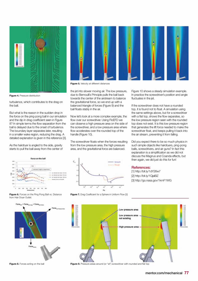
mentor.com/mechanical 77
turbulence, which contributes to the drag on the ball.
But what is the reason in the sudden drop in the force on the ping-pong ball in our simulation and the dip in drag coefficient seen in Figure 8? In simple terms the flow separation from the ball is delayed due to the onset of turbulence. The boundary layer separates later, resulting in a smaller wake region, reducing the drag. A detailed explanation is given in the reference [3].
As the hairdryer is angled to the side, gravity starts to pull the ball away from the center of
the jet into slower moving air. The low pressure, due to Bernoulli’s Principle pulls the ball back towards the center of the airstream to balance the gravitational force, so we end up with a balanced triangle of forces (Figure 9) and the ball floats stably in the air.
Now let’s look at a more complex example, the flow over our screwdriver. Using FloEFD we can observe a high pressure area on the side of the screwdriver, and a low pressure area where flow accelerates over the rounded top of the handle (Figure 10). The screwdriver floats when the forces resulting from the low pressure area, the high pressure area, and the gravitational force are balanced.
Figure 10 shows a steady simulation example. In practice the screwdriver’s position and angle fluctuates in the jet.
If the screwdriver does not have a rounded top, it is found not to float. A simulation using the same settings above, but for a screwdriver with a flat top, shows the flow separates, so the low pressure region seen with the rounded top does not exist. It is this low pressure region that generates the lift force needed to make the screwdriver float, and keeps pulling it back into the air stream, preventing it from falling.
Did you expect there to be so much physics in such simple objects like hairdryers, ping-pong balls, screwdrivers, and air guns? In fact this explanation is a simplification as we did not discuss the Magnus and Coanda effects, but then again, we did just do this for fun!
References:[1] http://bit.ly/1dY26w7
[2] http://bit.ly/1QjalBZ
[3] http://go.nasa.gov/1kmF1WG
Figure 4. Pressure distribution
Figure 5. Velocity at different distances
Figure 8. Forces acting on the ball Figure 9. Pressure areas around (or “at”) screwdriver with rounded and flat top
Figure 6. Forces on the Ping Pong Ball vs. Distance from Hair Dryer Outlet.
Figure 7. Drag Coefficient for a Sphere in Uniform Flow [3]

78 mentor.com/mechanical
Brownian Motion...The random musings of a Fluid Dynamicist
’ve just put down an interesting article which I’ll sum up for you in one easy sentence: you don’t need as much sleep as you think you do. Turns
out that this 8 hours per night thing is nonsense likely made up by a sleep aid manufacturer. For all our angst about the internet and blue-light devices keeping us up at night, the fact is that our distant ancestors were just as awake after sun down fixing spears and worrying about their end of quarter mammoth target.
The unholy alliance between marketing and ‘woo’ science is a widely covered topic but constant vigilance is nonetheless required! I’ve just had a long (in every sense of the word) taxi journey during which my driver tried to convince me of the benefits of a certain type of alternative medicine. I ventured that perhaps the reason it was alternative medicine, and not just medicine, was because there was no evidence that it worked. Not so, he claimed, I only had to look at the videos on YouTube. He had me there.
I’ve fallen victim to such logic failures myself, ironically when I was sleep deprived: it turns out that the reason my first child wasn’t sleeping wasn’t because I had money burning a hole in my wallet, it was because he was
I
Brownian Motion or Pedesis (from Greek: πήδησις Pɛɖeːsɪs 'leaping') is the presumably random moving of particles suspended in a fluid (a liquid or a gas) resulting from their bombardment by the fast-moving atoms or molecules in the gas or liquid. The term 'Brownian Motion' can also refer to the mathematical model used to describe such random movements, which is often called a particle theory.
a baby. That wasn’t covered in the article by the way; beyond a certain limit of tiredness credulity increases dramatically.
Anyway, the point is that constant vigilance is required my friends. 99% it’s just a matter
of not spending more money than you need to, but the fatter end of this nonsense wedge could be the stuff government policy is made of. And that’s a thought that should keep you awake at night. Turbulent Eddy
This article wouldn't have happened in my day!

mentor.com/mechanical 79
• 30 Day Instant Free Access to Full Software
• No License Set-up Required
• Each VLab contains Full Support Material
• 4 Hour Sessions*
• Save Work between Sessions
*These sessions can be extended
FloEFD™ for PTC CreoTest-drive 20 Powerful CFD Models including LED Thermal Characterization, CPU Cooling, Hydraulic Loss Determination, and more
go.mentor.com/floefd-vl
Flowmaster® Build & Analyze a Rising Main Network in Flowmaster
go.mentor.com/flowmaster-vl
Virtual Labswww.mentor.com/mechanical
REGISTER NOW for your instant 30 Day
Free Trialwww.mentor.com/mechanical
LED Analysis with FloEFD for PTC Creo Analyze LED Components & Determine Thermal Characteristics
go.mentor.com/floefd-led-vl
FloTHERM® XT CAD-centric thermal CFD from conceptual design to manufacture
go.mentor.com/flothermxt-vlab
NEW