EDFI 6450 Using Assessment & Research to Improve Practice

Page 1

EDFI 6450 Using Assessment & Research to Improve

Practice Course Packet

Dr. Rachel Vannatta Reinhart

Table of Contents

Week 1—Introduction to Standardized Testing .................................2 Week 2—Criterion-Referenced Test Scores .......................................6

Validity and Reliability ..................................................................7 Week 3—Descriptive Statistics (Video #2).......................................10 Week 4—Probability & z Scores (Video #3) ......................................17 Week 5— Norm-Referenced Test Scores (Video #4).................... 22 Week 6—Group & Student Level Decision Making (Video #5)...... 28

Online Assessment Resources.................................................. 35 Week 7—Value-Added Analysis ............................................................ 40 Week 9—Introduction to Inferential Statistics (Video #7)........ 46

Distribution of Sample Means.................................................. 50 Week 10—Hypothesis Testing (Video #8)......................................... 54

t Test of Single Sample..............................................................61 Week 11—t Test of Independent Samples (Video #9) ................... 66 t Test of Related Samples........................................................ 67 Week 12—AVOVA (Video #10)............................................................. 72 Week 13—Correlation & Regression (Video #11).............................. 77 Unit Normal (z-score) Table.................................................................. 85

Page 2

Week 1: Standardized Testing Introduction to Standardized Tests (ISTS 1) • A standardized test is one that is administered, scored, and interpreted in identical fashion for all examinees. • Standardized tests allow educators to gain a sense of the average level of performance for a well-defined group

of students. • Classroom teachers have no control over these types of tests, but must understand their nature and

interpretation. • Achievement tests measure academic skills. • Aptitude tests measure potential or future achievement. • Diagnostic tests are specialized achievement test to identify areas of strengths and weaknesses • Nationally known standardized tests include:

• California Achievement Test (CAT) • Comprehensive Test of Basic Skills (CTBS) • Iowa Test of Basic Skills (ITBS)

• Many states also use state-mandated tests, authorized by state legislatures or boards of education; used as high school grad requirements.

• Two types of standardized tests are norm-referenced (no predetermined passing score; performance is based on comparisons to others) and criterion-referenced (performance is compared to preestablished criteria).

• Today, test publishers are incorporating both norm-referenced and criterion-referenced scores so that a student’s achievement may be compared to the norm as well as the content standards/criteria.

A little More on Aptitude vs. Achievement

These two types of standardized tests are often used as if they were interchangeable, but they are very, very different.

Achievement Tests—Designed to measure mastery - what the student has learned in the past and what the student can perform in the present (e.g., Ohio Achievement Tests, ITBS, FCAT).

o Achievement tests measure what a student can do right now, today. o Asks about content area (e.g. math, reading) in order to understand a student’s content area skills. o The OATs are Achievement Tests which are linked to the state standards. Their objective is to

measure how much content a student has mastered in various content areas (math, reading, writing, social studies, science).

Aptitude Tests—Designed to measure how much promise a student has for the future. Specifically, predicting the future statistically (Scholastic Aptitude Test—SAT, ACT, PSAT).

o All of these tests are used to “predict” something in the future about the people who take the test—NOT to indicate current achievement.

o Asks about content area (e.g. math, reading) only because that content is universally known and only if people who answer the items correctly generally have more of the predicted trait.

o Aptitude tests try to predict something based on the answers. For example, if we are trying to predict who will make a good engineer we might test content areas such as logic, problem solving, math, and science. But we probably will not social studies because scoring high in this area would not likely predict well who would make a good engineer.

o SAT (Scholastic Aptitude Test) measures Math, Reading, Writing, Critical Reading skills. What do you suppose the SAT is trying to predict?

The SAT’s sole purpose is to predict the likelihood that a student will complete a 4-year degree.

The higher a person scores on the SAT the more likely they are to complete a 4-year college degree.

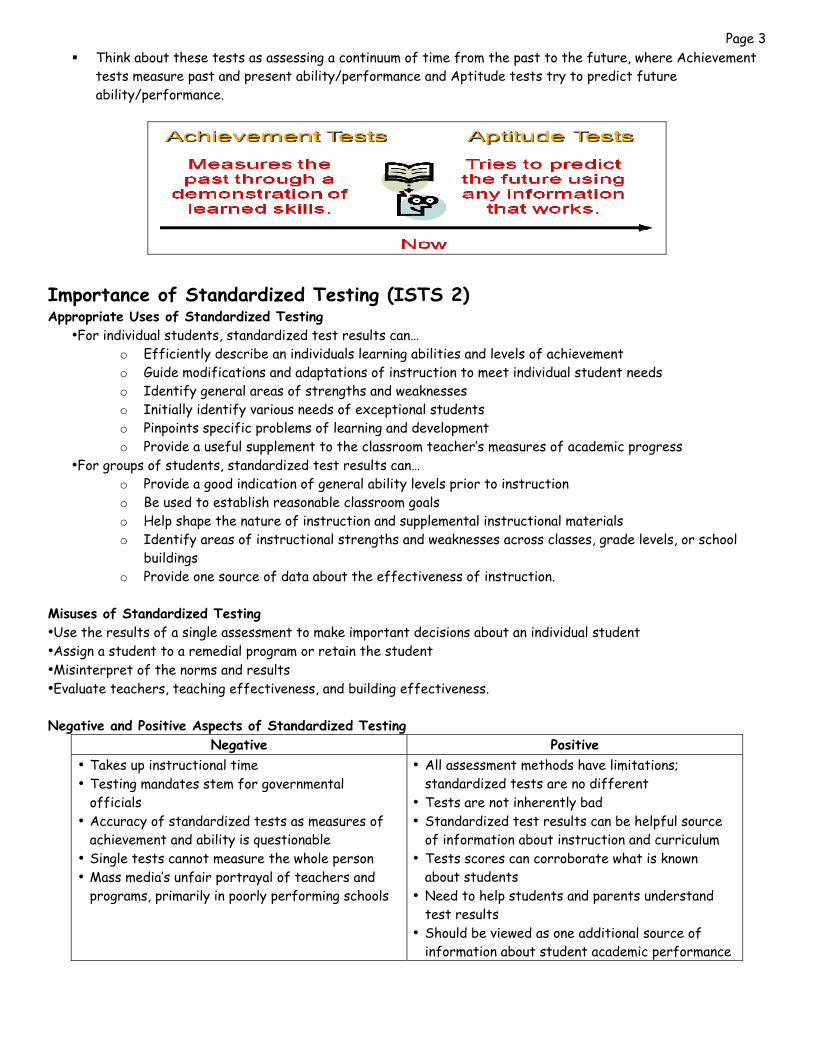
Page 3 Think about these tests as assessing a continuum of time from the past to the future, where Achievement

tests measure past and present ability/performance and Aptitude tests try to predict future ability/performance.

Importance of Standardized Testing (ISTS 2) Appropriate Uses of Standardized Testing

•For individual students, standardized test results can… o Efficiently describe an individuals learning abilities and levels of achievement o Guide modifications and adaptations of instruction to meet individual student needs o Identify general areas of strengths and weaknesses o Initially identify various needs of exceptional students o Pinpoints specific problems of learning and development o Provide a useful supplement to the classroom teacher’s measures of academic progress

•For groups of students, standardized test results can… o Provide a good indication of general ability levels prior to instruction o Be used to establish reasonable classroom goals o Help shape the nature of instruction and supplemental instructional materials o Identify areas of instructional strengths and weaknesses across classes, grade levels, or school

buildings o Provide one source of data about the effectiveness of instruction.

Misuses of Standardized Testing •Use the results of a single assessment to make important decisions about an individual student •Assign a student to a remedial program or retain the student •Misinterpret of the norms and results •Evaluate teachers, teaching effectiveness, and building effectiveness. Negative and Positive Aspects of Standardized Testing

Negative Positive • Takes up instructional time • Testing mandates stem for governmental

officials • Accuracy of standardized tests as measures of

achievement and ability is questionable • Single tests cannot measure the whole person • Mass media’s unfair portrayal of teachers and

programs, primarily in poorly performing schools

• All assessment methods have limitations; standardized tests are no different

• Tests are not inherently bad • Standardized test results can be helpful source

of information about instruction and curriculum • Tests scores can corroborate what is known

about students • Need to help students and parents understand

test results • Should be viewed as one additional source of

information about student academic performance

Page 4

Standardized Test Administration and Preparation (ISTS 3) Recommendations for Test Administration • Motivate students—explain purpose of test and how results will be used; be positive. • Follow directions STRICTLY—don’t paraphrase; only answer student questions regarding test directions and

procedures; don’t give hints toward answers. • Keep time accurately. • Record significant events—unusual student behavior or event that could influence test scores. • Collect test materials promptly. Testwiseness Skills Students should be taught or given the opportunity to practice the following:

• Listening/reading test directions and practice marking answer sheets • Listening/reading test items • Establishing pace that will permit test completion • Skipping difficult items and returning to the later • Making informed guesses for items that appear too difficult • Eliminating possible options (for multiple choice) • Checking to make sure that the answer number matches the item number • Checking answers and answer markings if time permits

Common Test Preparation Practices • Curriculum and test content—teaching the content that is addressed in the assessment—it is NOT teaching to

the test! • Assessment and item formats—provide student practice with item formats that they will encounter on the

assessment. • Test-taking strategies or Testwiseness Skills • Timing of test preparation—don’t cram; spread out preparation activities throughout the school year. • Student motivation—encourage students to perform their best.

Page 5 Student Test Preparation Do’s and Don’ts

Page 6

Week 2: Criterion-Referenced Tests, Validity & Reliability Criterion-Referenced Tests (ISTS 5)

• Permit teachers to draw inferences about what students can do relative to large domain regarding specific content.

• Scores represent the degree of accuracy with which a student has master specific content—is not dependent on the performance of others.

• Answer the following questions: • What does this student know? • What can this student do? What content and skills has the student mastered?

• Types of Criterion-Referenced Test Items • Selected-response items (multiple choice, true/false)

• Only one response is correct • Constructed-response items

• Requires student to recall information and create a response • Uses open-ended or performance-type items • Scoring is more subjective, but applies a list of criteria (rubric) to guide the scoring process

• Types of Criterion-Referenced Scores

• Raw scores, usually in the form of number or percentage of items answered correctly. • Other, less common results include speed of performance, quality of performance, and precision of

performance. • Cut Scores—to place a student in a Performance Category that is based upon some predetermined

standard of performance. For example, pass/fail; not proficient/proficient/ advanced; novice/basic/ proficient/ advanced.

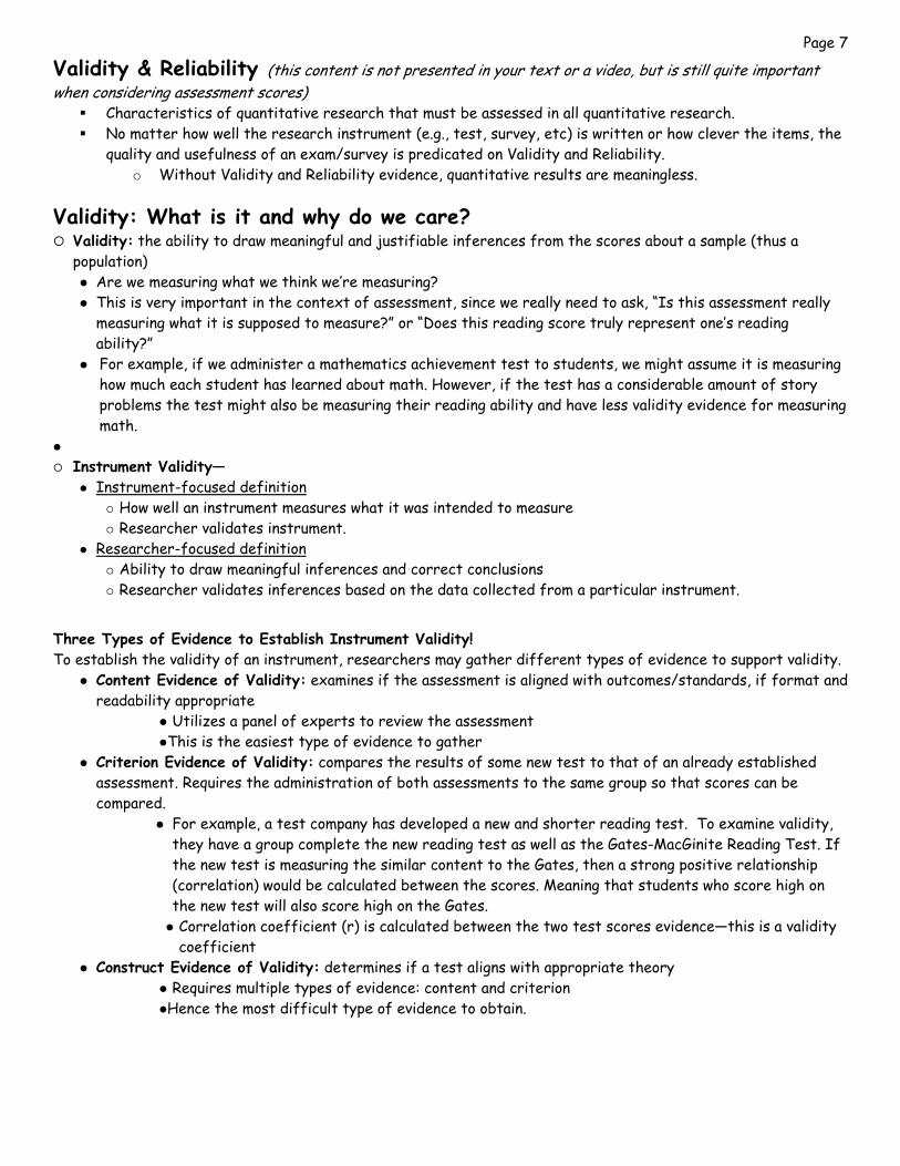
• Process of determining cut scores is standard setting. A Comparison of Criterion versus Norm-Referenced Tests

Criterion-Referenced Norm Referenced What does the student know? What content has the student mastered? How well did Johnny do on the Math test?

How does this student compare to other students who took this test? How well did Johnny do compared to Jill?

Student’s score is NOT compared to or dependent on other students’ scores. All students could get a passing score.

Student’s score IS compared to and dependent on other students’ (norm group) scores. 50% students above/below midpoint.

Have a predetermined “cut” score. OAT “cut” score for proficient is 400.

No predetermined pass/fail score. Performance rank depends on norm group.

Able to identify specific content the student needs help with. Student needs help with synonyms & antonyms.

Able to compare achievement across different subjects. Student is stronger in reading than math.

Page 7

Validity & Reliability (this content is not presented in your text or a video, but is still quite important when considering assessment scores)

Characteristics of quantitative research that must be assessed in all quantitative research. No matter how well the research instrument (e.g., test, survey, etc) is written or how clever the items, the

quality and usefulness of an exam/survey is predicated on Validity and Reliability. o Without Validity and Reliability evidence, quantitative results are meaningless.

Validity: What is it and why do we care? Validity: the ability to draw meaningful and justifiable inferences from the scores about a sample (thus a population)

Are we measuring what we think we’re measuring? This is very important in the context of assessment, since we really need to ask, “Is this assessment really measuring what it is supposed to measure?” or “Does this reading score truly represent one’s reading ability?”

For example, if we administer a mathematics achievement test to students, we might assume it is measuring how much each student has learned about math. However, if the test has a considerable amount of story problems the test might also be measuring their reading ability and have less validity evidence for measuring math.

Instrument Validity—

Instrument-focused definition How well an instrument measures what it was intended to measure Researcher validates instrument.

Researcher-focused definition Ability to draw meaningful inferences and correct conclusions Researcher validates inferences based on the data collected from a particular instrument.

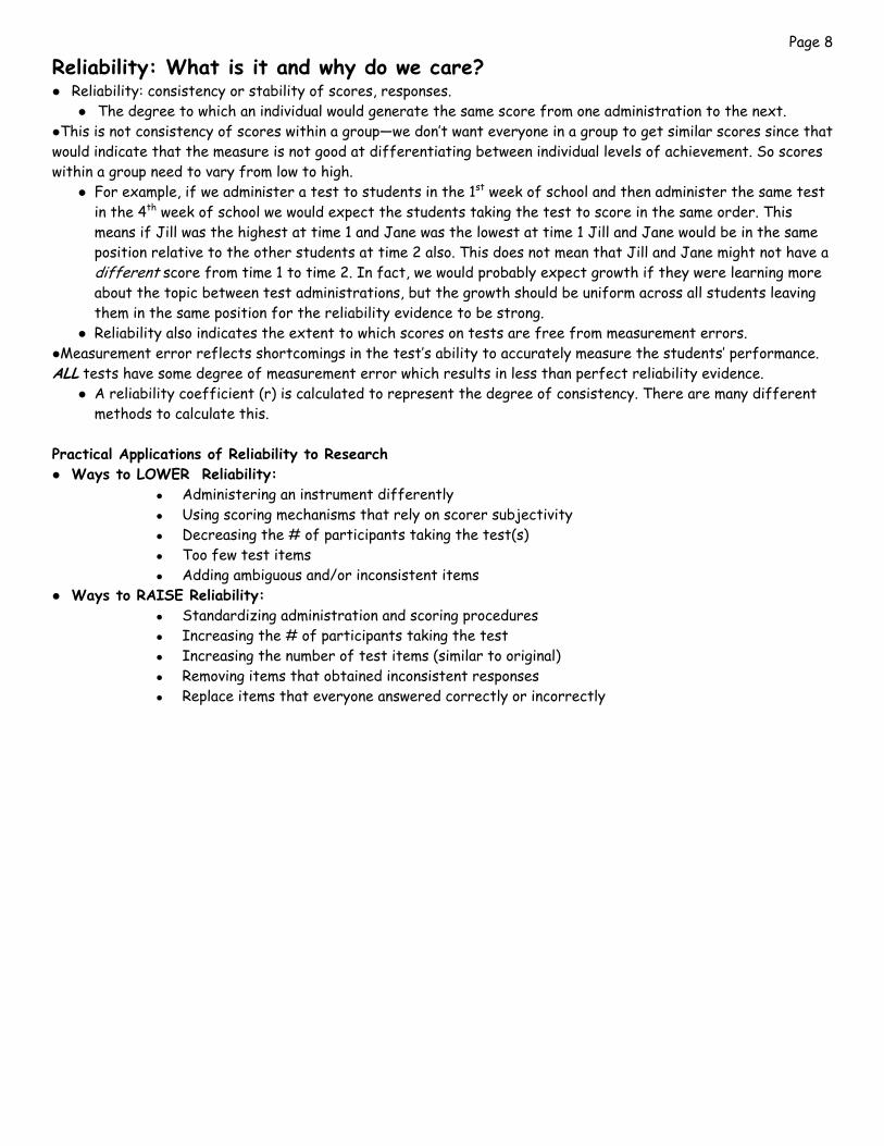
Three Types of Evidence to Establish Instrument Validity! To establish the validity of an instrument, researchers may gather different types of evidence to support validity.

Content Evidence of Validity: examines if the assessment is aligned with outcomes/standards, if format and readability appropriate

Utilizes a panel of experts to review the assessment This is the easiest type of evidence to gather

Criterion Evidence of Validity: compares the results of some new test to that of an already established assessment. Requires the administration of both assessments to the same group so that scores can be compared.

For example, a test company has developed a new and shorter reading test. To examine validity, they have a group complete the new reading test as well as the Gates-MacGinite Reading Test. If the new test is measuring the similar content to the Gates, then a strong positive relationship (correlation) would be calculated between the scores. Meaning that students who score high on the new test will also score high on the Gates. Correlation coefficient (r) is calculated between the two test scores evidence—this is a validity coefficient

Construct Evidence of Validity: determines if a test aligns with appropriate theory Requires multiple types of evidence: content and criterion Hence the most difficult type of evidence to obtain.

Page 8

Reliability: What is it and why do we care? Reliability: consistency or stability of scores, responses.

The degree to which an individual would generate the same score from one administration to the next. This is not consistency of scores within a group—we don’t want everyone in a group to get similar scores since that

would indicate that the measure is not good at differentiating between individual levels of achievement. So scores within a group need to vary from low to high.

For example, if we administer a test to students in the 1st week of school and then administer the same test in the 4th week of school we would expect the students taking the test to score in the same order. This means if Jill was the highest at time 1 and Jane was the lowest at time 1 Jill and Jane would be in the same position relative to the other students at time 2 also. This does not mean that Jill and Jane might not have a different score from time 1 to time 2. In fact, we would probably expect growth if they were learning more about the topic between test administrations, but the growth should be uniform across all students leaving them in the same position for the reliability evidence to be strong.

Reliability also indicates the extent to which scores on tests are free from measurement errors. Measurement error reflects shortcomings in the test’s ability to accurately measure the students’ performance.

ALL tests have some degree of measurement error which results in less than perfect reliability evidence. A reliability coefficient (r) is calculated to represent the degree of consistency. There are many different methods to calculate this.

Practical Applications of Reliability to Research

Ways to LOWER Reliability: Administering an instrument differently Using scoring mechanisms that rely on scorer subjectivity Decreasing the # of participants taking the test(s) Too few test items Adding ambiguous and/or inconsistent items

Ways to RAISE Reliability: Standardizing administration and scoring procedures Increasing the # of participants taking the test Increasing the number of test items (similar to original) Removing items that obtained inconsistent responses Replace items that everyone answered correctly or incorrectly

Page 9 Relationship between Validity and Reliability

Reliability and validity are related!!! See targets below: Let’s assume that hitting the target is validity, and having our arrows cluster

together is reliability (consistency)

Reliable Valid

Reliable Invalid

Unreliable Invalid

The arrows have “consistently” hit the

“target”. Therefore, we are consistently measuring the information we were hoping

to measure!

The arrows are “consistent in hitting the same location, but

they have NOT “hit the target.” Therefore, we are consistently measuring the

WRONG information.

The arrows are all over the place so they are not

consistent. They have not hit the target. Therefore,

we are inconsistently measuring the WRONG

information. This is a super BAD test!

Conclusion?

In order to have validity, you MUST have reliability! However, reliability doesn’t ensure validity!

Page 10

Week 3 Video #2: Descriptive Statistics

Video #2a: Introduction to Descriptive Statistics and

Measures of Central Tendencies Descriptive Statistics •Summarize, organize and simplify data to “describe the sample”

•Measures of Central Tendencies •Measures of Variability •Frequencies •Tables •Graphs and plots

• Measures of central tendency and variability create the basis for the normal distribution, which is the foundation of standardized testing!

Statistical Notation f = frequency Σ = sum of X = individual score N = number in population n = number in sample M or X = mean for sample μ = mean for population s or SD = standard deviation for sample σ = standard deviation for Measure of Central Tendency

• describes a group of individuals with a single measurement that is most representative of all individuals • Types: mean, median, and mode

• Mean—arithmetic average

• used for interval/ratio (quantitative) data • computed by adding all the scores and dividing by the number of scores (N = # in population, n = # in

sample) • Population mean = μ = ΣX Sample mean = X or M = ΣX

N n • Sample mean in publications is often represented by M

• Median—the midpoint; the score that divides the distribution exactly in half; 50% are above and below the median

• used for ordinal data or when: there is a skewed distribution, some scores are undetermined, or there is an open-ended distribution

• Calculating the median when N is an odd number • make sure scores are in order; find the middle score

• Calculating the median when N is an even number • make sure scores are in order; find the two middle scores; add the two scores & divide by 2

Page 11 • Mode—the most frequent score

• used especially for nominal data • represented by the highest point in the frequency distribution

Central Tendency and the Shape of Distributions • Normal distribution—mean, median, and mode are equal and smack-dab in the middle of a bell-curve distribution

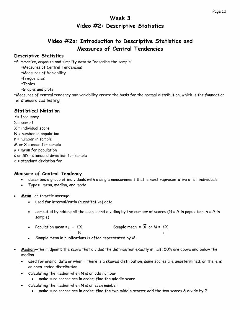
• Skewed Distributions • not symmetrical • mean, median, mode are different • extreme scores on one end of the distribution • Mean is most affected by extreme scores, so it will be furthest out in the tail

Negatively Skewed—extreme scores are on the low end of the distribution

Mean Median Mode Positively Skewed—extreme scores are on the high end of the distribution

Mode Median Mean

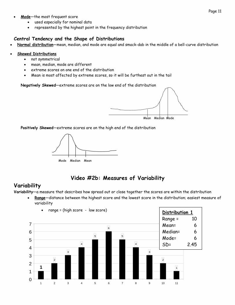
Video #2b: Measures of Variability Variability Variability—a measure that describes how spread out or close together the scores are within the distribution

• Range—distance between the highest score and the lowest score in the distribution; easiest measure of variability

• range = (high score - low score)

1

2

3

4

5

6

5

4

3

2

1

0

1

2

3

4

5

6

7

1 2 3 4 5 6 7 8 9 10 11

Distribution 1 Range = 10 Mean= 6 Median= 6 Mode= 6 SD= 2.45

Page 12

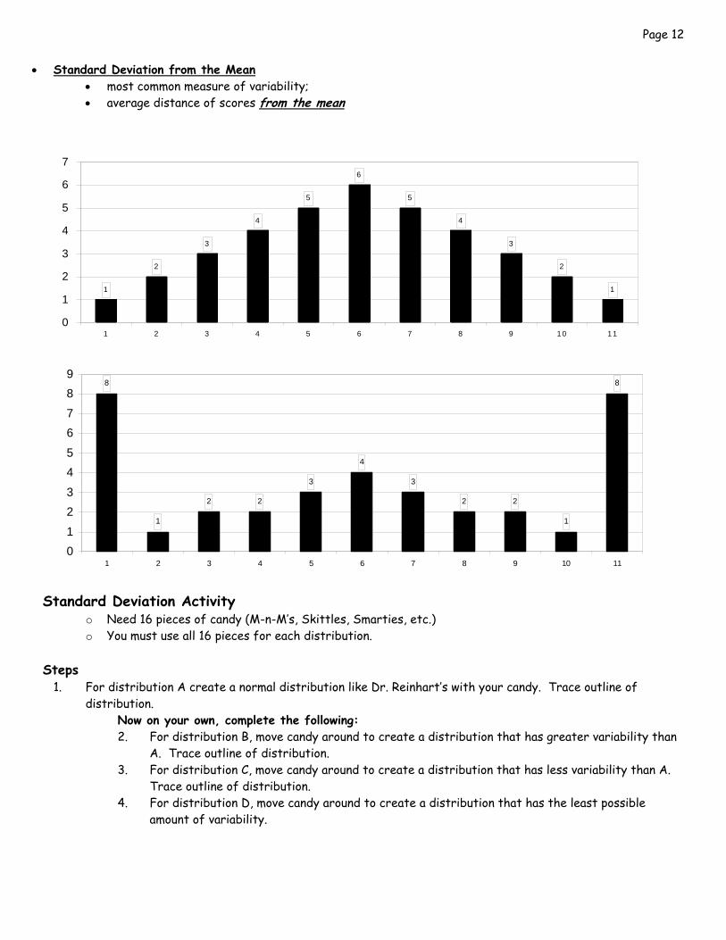
• Standard Deviation from the Mean • most common measure of variability; • average distance of scores from the mean

Distribution #2 Standard Deviation Activity

o Need 16 pieces of candy (M-n-M’s, Skittles, Smarties, etc.) o You must use all 16 pieces for each distribution.

Steps

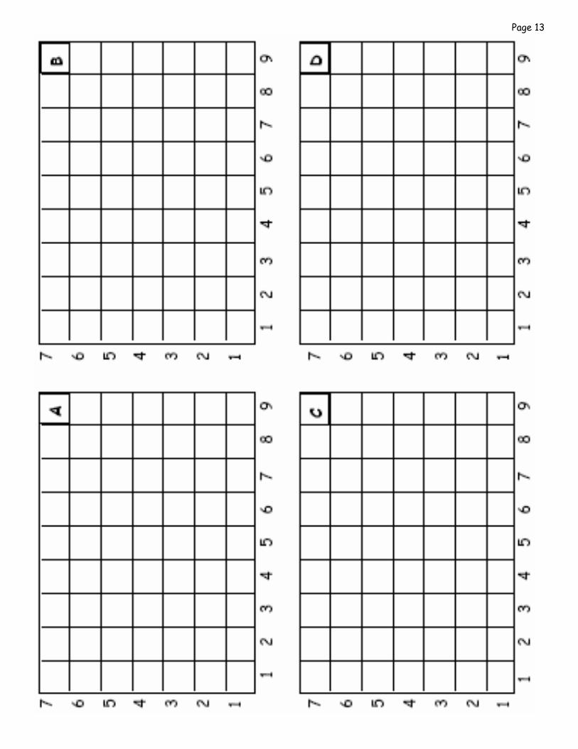
1. For distribution A create a normal distribution like Dr. Reinhart’s with your candy. Trace outline of distribution.

Now on your own, complete the following: 2. For distribution B, move candy around to create a distribution that has greater variability than

A. Trace outline of distribution. 3. For distribution C, move candy around to create a distribution that has less variability than A.

Trace outline of distribution. 4. For distribution D, move candy around to create a distribution that has the least possible

amount of variability.

8

1

2 2

3

4

3

2 2

1

8

01

23

45

67

89

1 2 3 4 5 6 7 8 9 10 11

1

2

3

4

5

6

5

4

3

2

1

0

1

2

3

4

5

6

7

1 2 3 4 5 6 7 8 9 1 0 1 1

Page 13

Page 14 Variability Key Concepts • Variability shows how spread out scores are in the distribution.

• Range only takes into account the two extreme scores (highest and lowest) • Standard deviation compares all scores to the mean

• When scores are close to the mean, then variability is less. • When scores are far from the mean (outliers, extreme ends of the distribution), then variability is more.

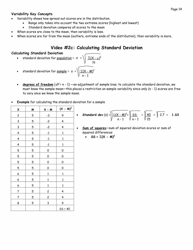
Video #2c: Calculating Standard Deviation

Calculating Standard Deviation • standard deviation for population = σ = Σ(X - μ)2

N

• standard deviation for sample = s = Σ(X - M)2 n - 1

• degrees of freedom (df = n - 1) —an adjustment of sample bias; to calculate the standard deviation, we must know the sample mean—this places a restriction on sample variability since only (n - 1) scores are free to vary once we know the sample mean.

• Example for calculating the standard deviation for a sample

• Standard dev (s) = Σ(X - M)2= SS = 40 = 2.7 = 1.63 n - 1 n – 1 15 • Sum of squares—sum of squared deviation scores or sum of

squared differences • SS = Σ(X - M)2

X M X - M (X - M)2

2 5 -3 9

3 5 -2 4

3 5 -2 4

4 5 -1 1

4 5 -1 1

4 5 -1 1

5 5 0 0

5 5 0 0

5 5 0 0

5 5 0 0

6 5 1 1

6 5 1 1

6 5 1 1

7 5 2 4

7 5 2 4

8 5 3 9

SS = 40

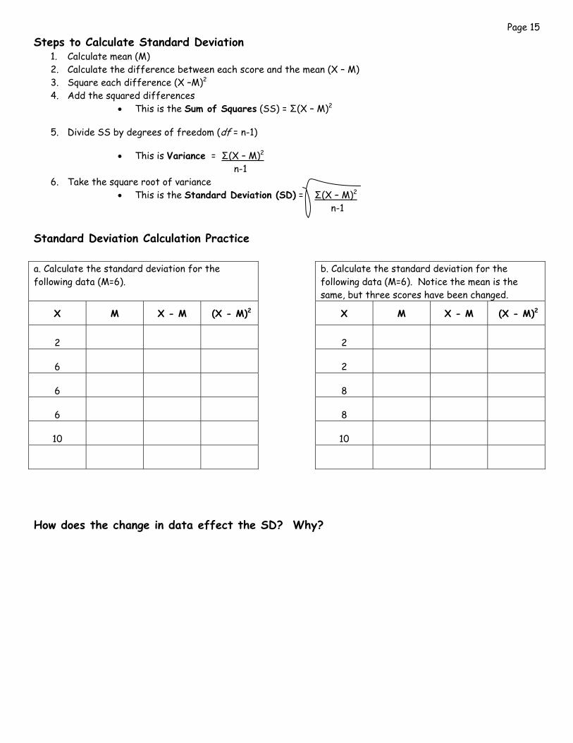
Page 15 Steps to Calculate Standard Deviation

1. Calculate mean (M) 2. Calculate the difference between each score and the mean (X – M) 3. Square each difference (X –M)2 4. Add the squared differences

• This is the Sum of Squares (SS) = Σ(X – M)2

5. Divide SS by degrees of freedom (df = n-1)

• This is Variance = Σ(X – M)2 n-1

6. Take the square root of variance • This is the Standard Deviation (SD) = Σ(X – M)2 n-1

Standard Deviation Calculation Practice a. Calculate the standard deviation for the following data (M=6). b. Calculate the standard deviation for the

following data (M=6). Notice the mean is the same, but three scores have been changed.

X M X - M (X - M)2 X M X - M (X - M)2

2 2 6 2 6 8 6 8 10 10

How does the change in data effect the SD? Why?

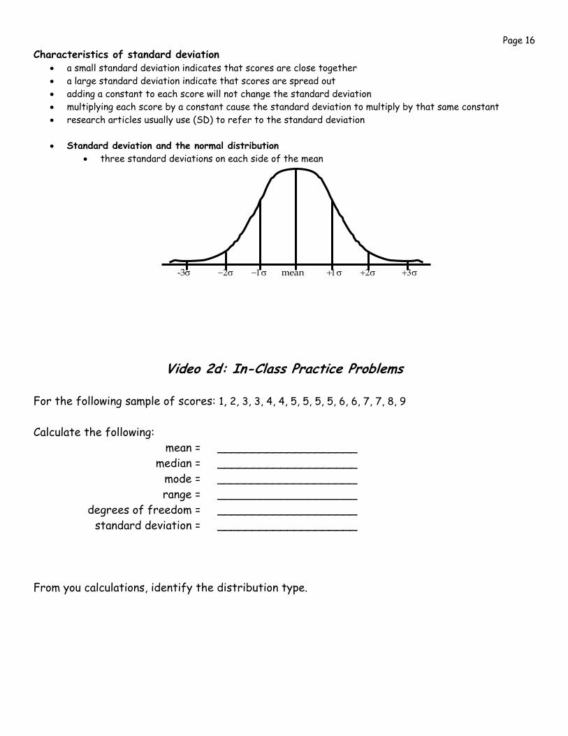
Page 16 Characteristics of standard deviation

• a small standard deviation indicates that scores are close together • a large standard deviation indicate that scores are spread out • adding a constant to each score will not change the standard deviation • multiplying each score by a constant cause the standard deviation to multiply by that same constant • research articles usually use (SD) to refer to the standard deviation • Standard deviation and the normal distribution

• three standard deviations on each side of the mean -3σ −2σ −1σ mean +1σ +2σ +3σ

Video 2d: In-Class Practice Problems

For the following sample of scores: 1, 2, 3, 3, 4, 4, 5, 5, 5, 5, 6, 6, 7, 7, 8, 9 Calculate the following: mean = ____________________ median = ____________________ mode = ____________________ range = ____________________ degrees of freedom = ____________________ standard deviation = ____________________

From you calculations, identify the distribution type.

Page 17

Week 4

Video #3: Probability and z-scores

Video #3a: Probability Probability is used to:

• determine the types of sample we are likely to obtain from a population • make conclusions about the population from the sample • Probability—fraction, proportion or percent of selecting a specific outcome out of the total number of

possible selections

• probability of A = number of A’s total number of possible outcomes

• probability of selecting a heart out of deck of cards • p (heart) = 13 = 1 = .25 25%

52 4

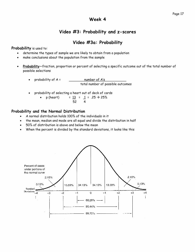
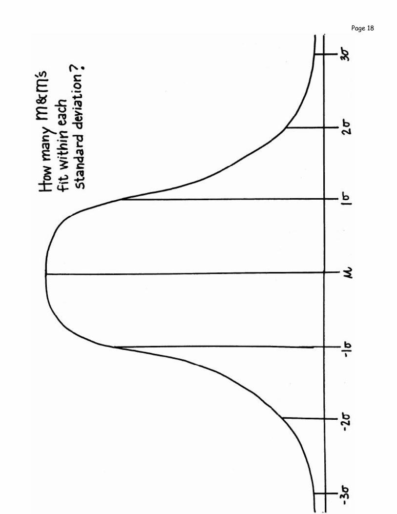
Probability and the Normal Distribution • A normal distribution holds 100% of the individuals in it • the mean, median and mode are all equal and divide the distribution in half • 50% of distribution is above and below the mean • When the percent is divided by the standard deviations, it looks like this

Page 18

Page 19

Video #3b: z Scores

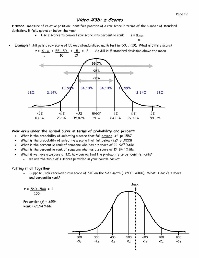
z score—measure of relative position; identifies position of a raw score in terms of the number of standard deviations it falls above or below the mean

• Use z scores to convert raw score into percentile rank z = X - μ σ

• Example: Jill gets a raw score of 55 on a standardized math test (μ=50, σ=10). What is Jill’s z score?

z = X - μ = 55 - 50 = 5 = .5 So Jill is .5 standard deviation above the mean. σ 10 10

99.7%

95%

68% 13.59% 34.13% 34.13% 13.59% .13% 2.14% 2.14% .13%

-3z -2z -3z mean 1z 2z 3z 0.13% 2.28% 15.87% 50% 84.13% 97.72% 99.87%

View area under the normal curve in terms of probability and percent: • What is the probability of selecting a score that fall beyond 1z? p=.1587 • What is the probability of selecting a score that fall below -2z? p=.0228 • What is the percentile rank of someone who has a z score of 2? 98th %tile • What is the percentile rank of someone who has a z score of 1? 84th %tile • What if we have a z-score of 1.2, how can we find the probability or percentile rank?

• we use the table of z scores provided in your course packet

Putting it all together • Suppose Jack receives a raw score of 540 on the SAT-math (μ=500, σ=100). What is Jack’s z score

and percentile rank?

Jack z = 540 - 500 = .4 100 Proportion (p) = .6554 Rank = 65.54 %tile

200 300 400 500 600 700 800 -3z -2z -1z 0z +1z +2z +3z

Page 20

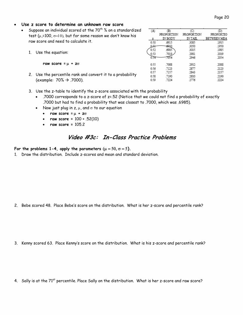
• Use z score to determine an unknown raw score • Suppose an individual scored at the 70th % on a standardized

test (μ,=100, σ=10), but for some reason we don’t know his raw score and need to calculate it.

1. Use the equation:

raw score = μ + zσ

2. Use the percentile rank and convert it to a probability

(example: 70% .7000).

3. Use the z-table to identify the z-score associated with the probability • .7000 corresponds to a z-score of z=.52 (Notice that we could not find a probability of exactly

.7000 but had to find a probability that was closest to .7000, which was .6985). • Now just plug in z, μ, and σ to our equation

• raw score = μ + zσ • raw score = 100 + .52(10) • raw score = 105.2

Video #3c: In-Class Practice Problems

For the problems 1-4, apply the parameters (μ = 50, σ = 5). 1. Draw the distribution. Include z-scores and mean and standard deviation. 2. Bebe scored 48. Place Bebe’s score on the distribution. What is her z-score and percentile rank?

3. Kenny scored 63. Place Kenny’s score on the distribution. What is his z-score and percentile rank?

4. Sally is at the 71st percentile. Place Sally on the distribution. What is her z-score and raw score?

Page 21

Additional Practice Problems

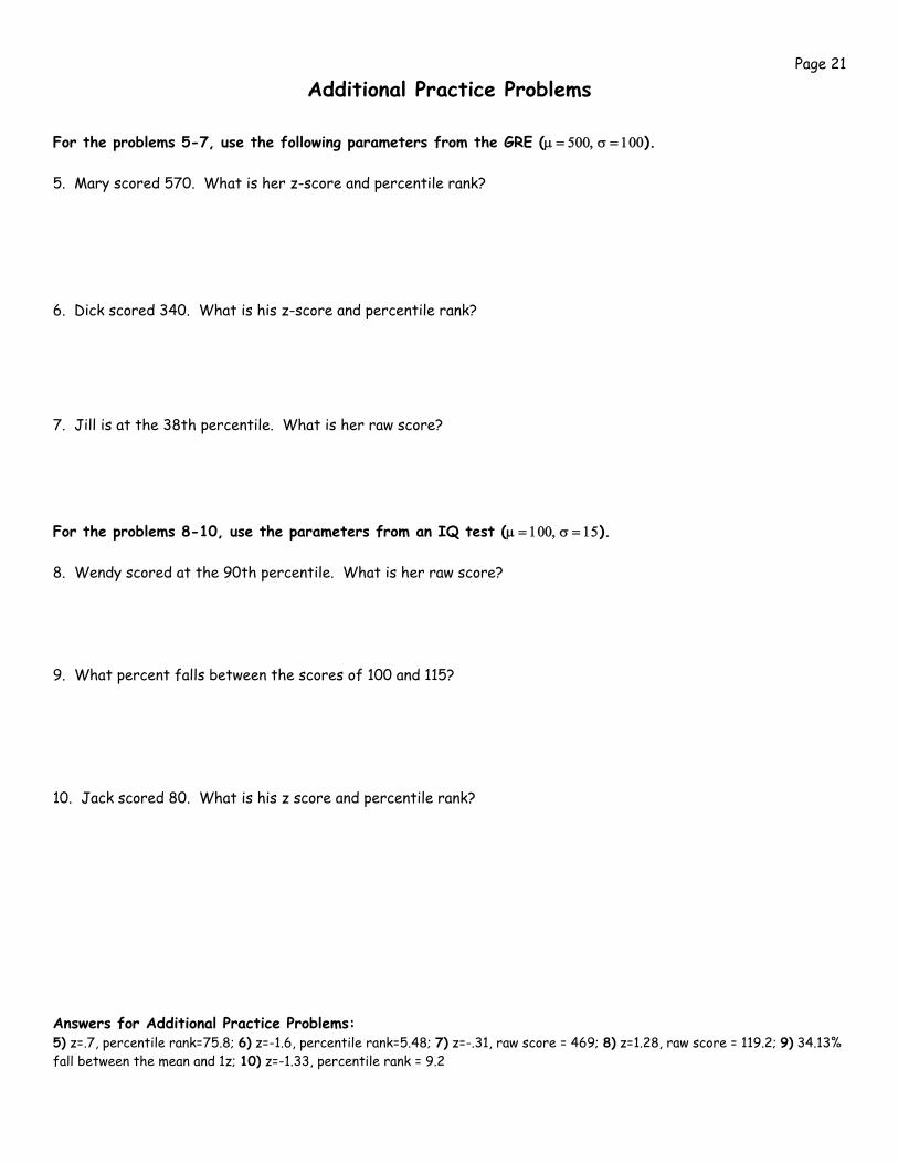
For the problems 5-7, use the following parameters from the GRE (μ = 500, σ = 100). 5. Mary scored 570. What is her z-score and percentile rank?

6. Dick scored 340. What is his z-score and percentile rank?

7. Jill is at the 38th percentile. What is her raw score?

For the problems 8-10, use the parameters from an IQ test (μ = 100, σ = 15). 8. Wendy scored at the 90th percentile. What is her raw score? 9. What percent falls between the scores of 100 and 115? 10. Jack scored 80. What is his z score and percentile rank? Answers for Additional Practice Problems: 5) z=.7, percentile rank=75.8; 6) z=-1.6, percentile rank=5.48; 7) z=-.31, raw score = 469; 8) z=1.28, raw score = 119.2; 9) 34.13% fall between the mean and 1z; 10) z=-1.33, percentile rank = 9.2

Page 22

Week 5

Video #4: Norm-Referenced Tests

Video #4a: Norm-Referenced Test Scores Norm-Referenced Tests

• Permit comparisons to well-defined norm group (intended to represent current level of achievement for a specific group of students at a specific grade level).

• Answer the following questions: • What is the relative standing of this student across this broad domain of content? • How does the student compare to other similar students?

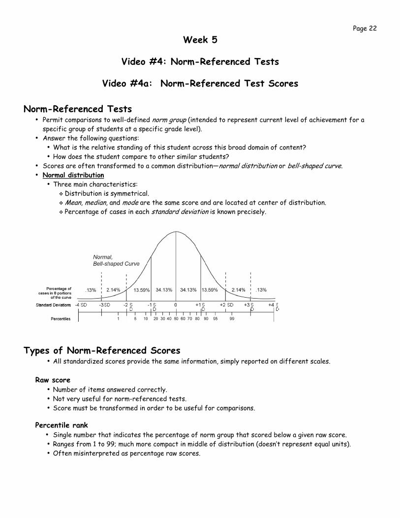
• Scores are often transformed to a common distribution—normal distribution or bell-shaped curve. • Normal distribution

• Three main characteristics: Distribution is symmetrical. Mean, median, and mode are the same score and are located at center of distribution. Percentage of cases in each standard deviation is known precisely.

Types of Norm-Referenced Scores

• All standardized scores provide the same information, simply reported on different scales.

Raw score • Number of items answered correctly. • Not very useful for norm-referenced tests. • Score must be transformed in order to be useful for comparisons.

Percentile rank

• Single number that indicates the percentage of norm group that scored below a given raw score. • Ranges from 1 to 99; much more compact in middle of distribution (doesn’t represent equal units). • Often misinterpreted as percentage raw scores.

Page 23

Linear Standard Scores

• Score that results from transformation to fit normal distribution. • Overcomes previous limitation of unequal units. • Allows for comparison of performance across two different measures. • Reports performance on various scales to determine how many standard deviations the score is away from

the mean.

z-score More than 99% of scores fall in the range of –3.00 to +3.00. Sign indicates whether above or below mean; number indicates how many standard deviations away from mean.

Half the students will be above; half will be below. Problems with interpreting negative scores.

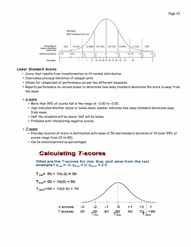
T-score

Provides location of score in distribution with mean of 50 and standard deviation of 10 (over 99% of scores range from 20 to 80).

Can be misinterpreted as percentages.

Page 24 Normalized Standard Score

SAT/GRE score Provides location of score in distribution with mean of 500 and standard deviation of 100 (over 99% of scores range from 200 to 800).

Deviation IQ score

Provides location of score in distribution with mean of 100 and standard deviation of 15 or 16. Primarily used with measures of mental ability.

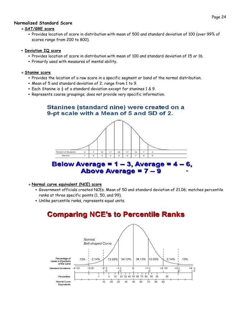
Stanine score

Provides the location of a raw score in a specific segment or band of the normal distribution. Mean of 5 and standard deviation of 2; range from 1 to 9. Each Stanine is ½ of a standard deviation except for stanines 1 & 9. Represents coarse groupings; does not provide very specific information.

Normal curve equivalent (NCE) score Government officials created NCEs. Mean of 50 and standard deviation of 21.06; matches percentile ranks at three specific points (1, 50, and 99).

Unlike percentile ranks, represents equal units.

Page 25 Developmental and Growth Scales • Grade-equivalent score: The grade in the norm group for which a certain raw score was the median

performance. • Consists of two numerical components: The first number indicates grade level and the second indicates

the month during that school year (ranges from 0 to 9); for example, grade-equivalent score of 4.2. • Often misinterpreted as standard to be achieved. • Although scores represent months, they do not represent equal units. o Example: Sally is in the 9th grade and receives a 7.8 GE on a standardized test.

o Sally’s score is a 7.8. The 7 tells us the grade level and the .8 tells us the month (0=September & 9=June). It is assumed a typical student will gain one unit of knowledge per month.

o Tests that provide Grade Level Equivalents scores give their test to multiple grade levels. Therefore, Sally scores the same on the 9th grade assessment as an average 7th grader would in their 8th month of school (May).

o This does not mean that Sally needs to be learning 7th grade material. We do not know how Sally would perform on a 7th grade test which tests 7th grade content. All we can say is that Sally likely needs remediation and is performing worse than her peers.

• Age-equivalent score: Based upon average test performance of students at various age levels.

• Consists of two numerical components: The first number indicates age in years, and the second indicates the month (ranges from 0 to 11);

• Does not represent equal units.

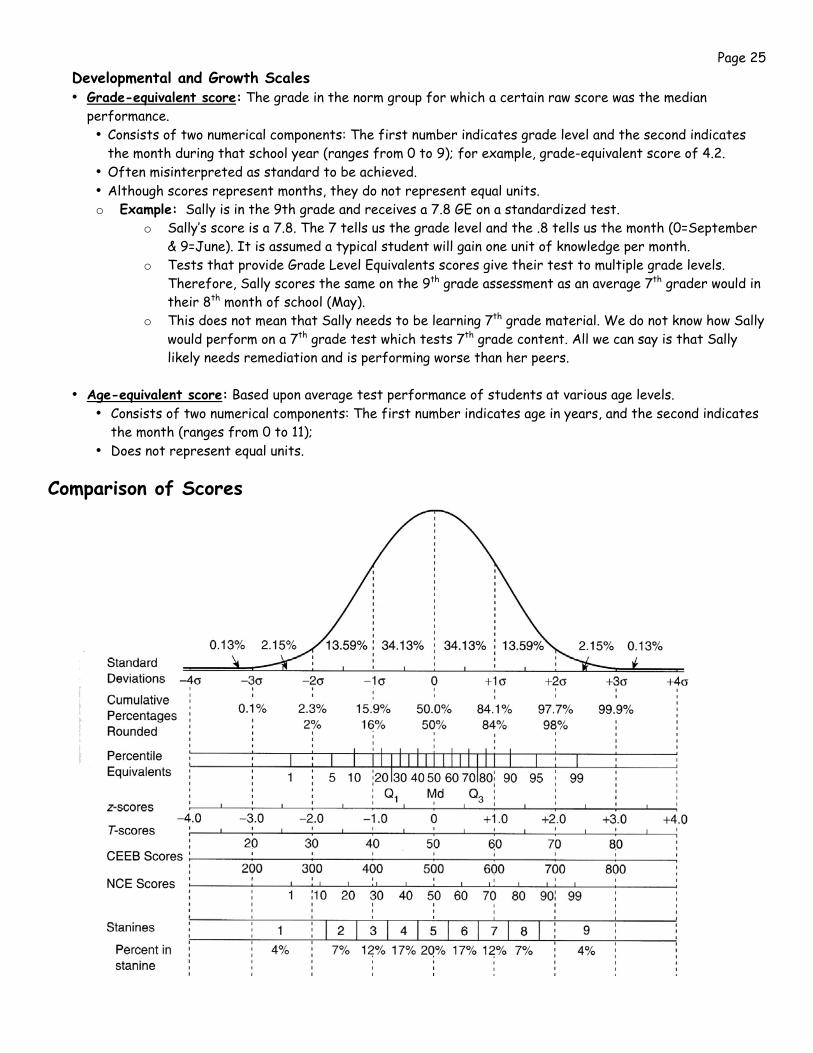
Comparison of Scores

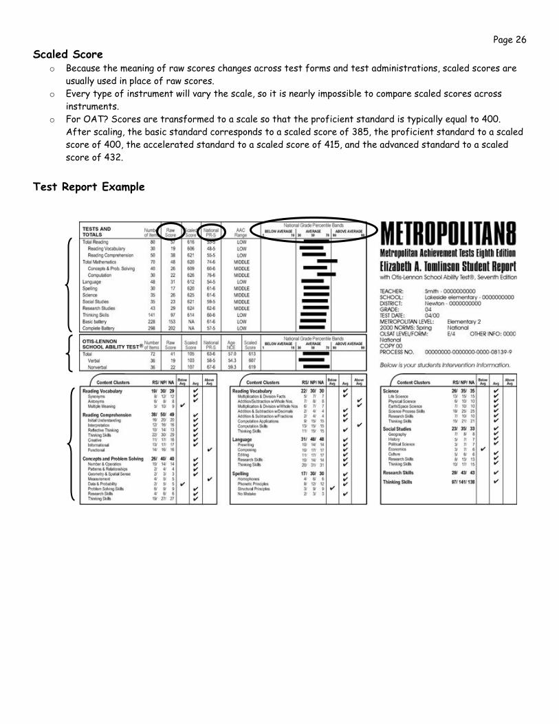
Page 26 Scaled Score

o Because the meaning of raw scores changes across test forms and test administrations, scaled scores are usually used in place of raw scores.

o Every type of instrument will vary the scale, so it is nearly impossible to compare scaled scores across instruments.

o For OAT? Scores are transformed to a scale so that the proficient standard is typically equal to 400. After scaling, the basic standard corresponds to a scaled score of 385, the proficient standard to a scaled score of 400, the accelerated standard to a scaled score of 415, and the advanced standard to a scaled score of 432.

Test Report Example

Page 27

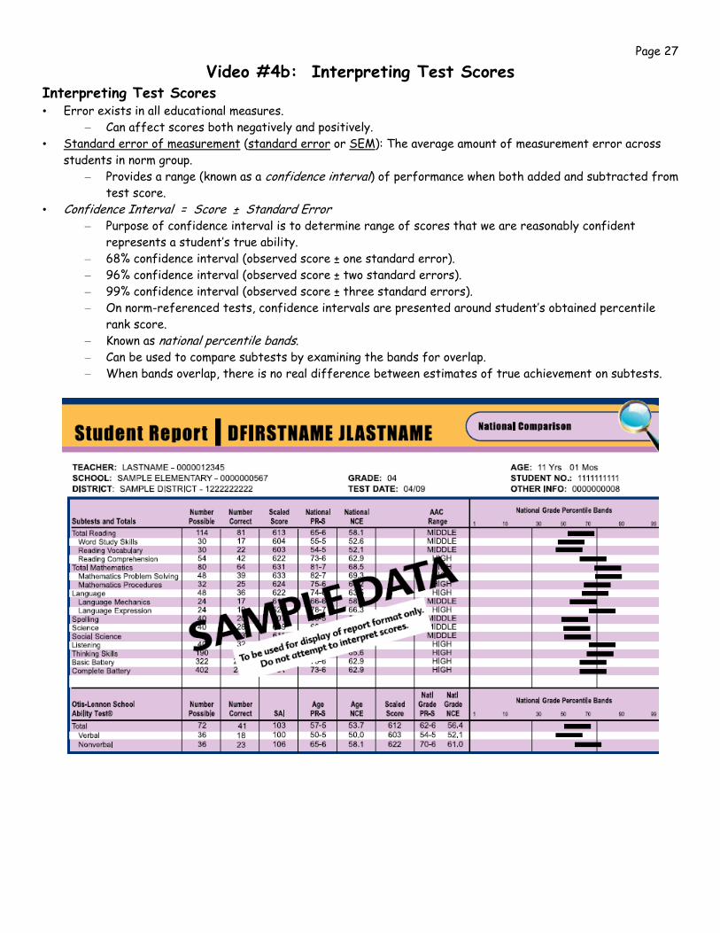
Video #4b: Interpreting Test Scores Interpreting Test Scores • Error exists in all educational measures.

– Can affect scores both negatively and positively. • Standard error of measurement (standard error or SEM): The average amount of measurement error across

students in norm group. – Provides a range (known as a confidence interval) of performance when both added and subtracted from

test score. • Confidence Interval = Score ± Standard Error

– Purpose of confidence interval is to determine range of scores that we are reasonably confident represents a student’s true ability.

– 68% confidence interval (observed score ± one standard error). – 96% confidence interval (observed score ± two standard errors). – 99% confidence interval (observed score ± three standard errors). – On norm-referenced tests, confidence intervals are presented around student’s obtained percentile

rank score. – Known as national percentile bands. – Can be used to compare subtests by examining the bands for overlap. – When bands overlap, there is no real difference between estimates of true achievement on subtests.

Page 28

Week 6

Video #5: Group and Student Level Decision Making (ISTS 7-8)

Video #5a: Group Level Decision Making

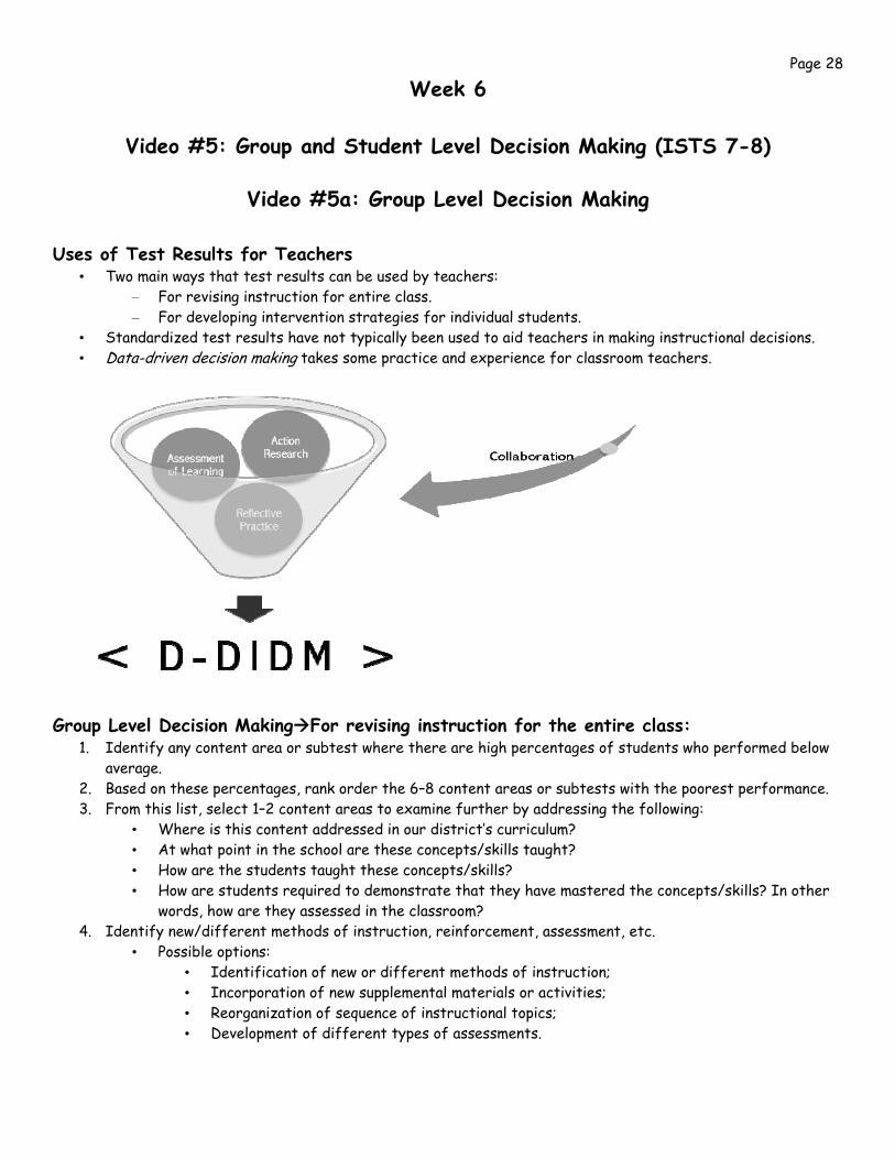
Uses of Test Results for Teachers • Two main ways that test results can be used by teachers:

– For revising instruction for entire class. – For developing intervention strategies for individual students.

• Standardized test results have not typically been used to aid teachers in making instructional decisions. • Data-driven decision making takes some practice and experience for classroom teachers.

Group Level Decision Making For revising instruction for the entire class:

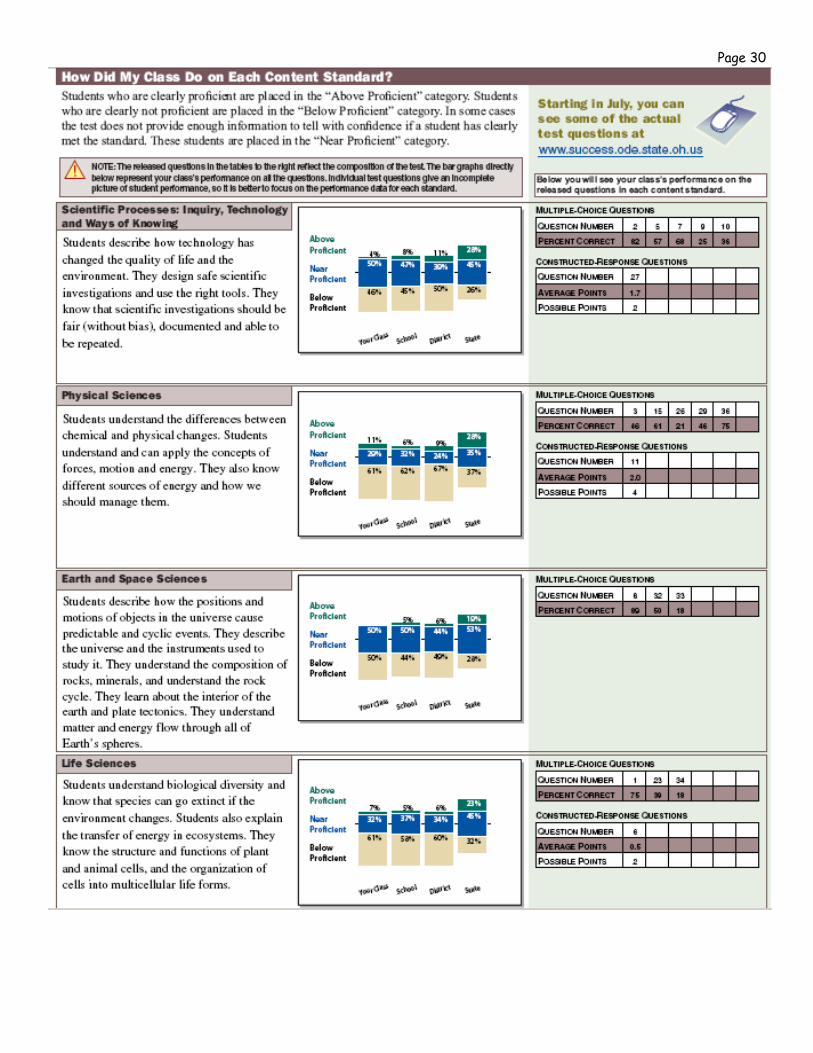
1. Identify any content area or subtest where there are high percentages of students who performed below average.

2. Based on these percentages, rank order the 6–8 content areas or subtests with the poorest performance. 3. From this list, select 1–2 content areas to examine further by addressing the following:

• Where is this content addressed in our district’s curriculum? • At what point in the school are these concepts/skills taught? • How are the students taught these concepts/skills? • How are students required to demonstrate that they have mastered the concepts/skills? In other

words, how are they assessed in the classroom? 4. Identify new/different methods of instruction, reinforcement, assessment, etc.

• Possible options: • Identification of new or different methods of instruction; • Incorporation of new supplemental materials or activities; • Reorganization of sequence of instructional topics; • Development of different types of assessments.

Page 29 Group Level Example

Your District

Your Name

Page 30

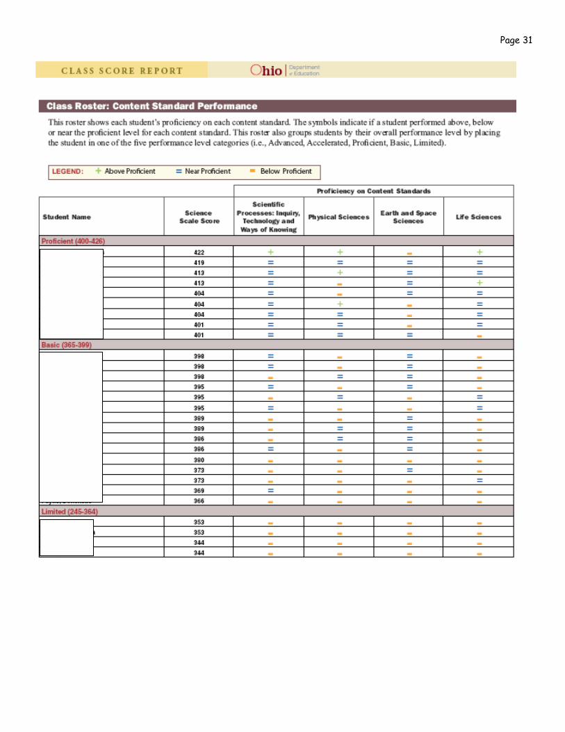
Page 31

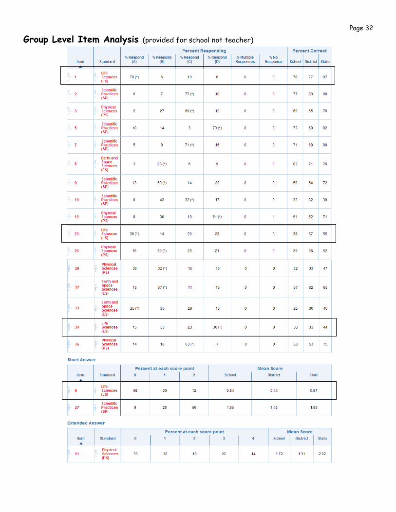
Page 32

Group Level Item Analysis (provided for school not teacher)

Page 33

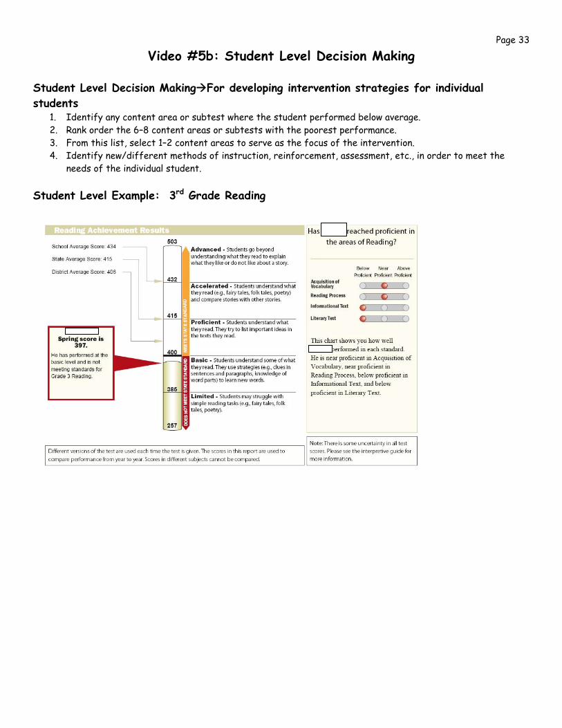
Video #5b: Student Level Decision Making Student Level Decision Making For developing intervention strategies for individual students

1. Identify any content area or subtest where the student performed below average. 2. Rank order the 6–8 content areas or subtests with the poorest performance. 3. From this list, select 1–2 content areas to serve as the focus of the intervention. 4. Identify new/different methods of instruction, reinforcement, assessment, etc., in order to meet the

needs of the individual student.

Student Level Example: 3rd Grade Reading

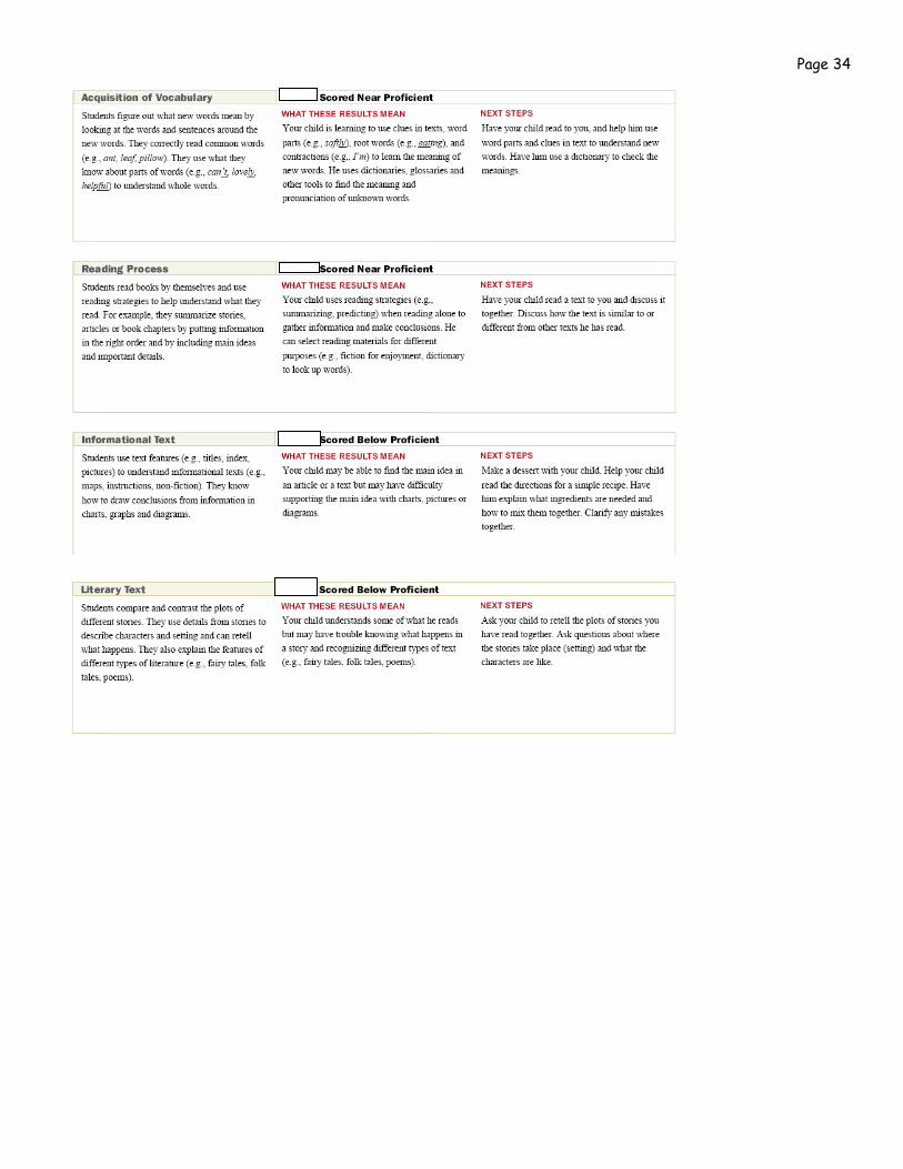
Page 34

Page 35

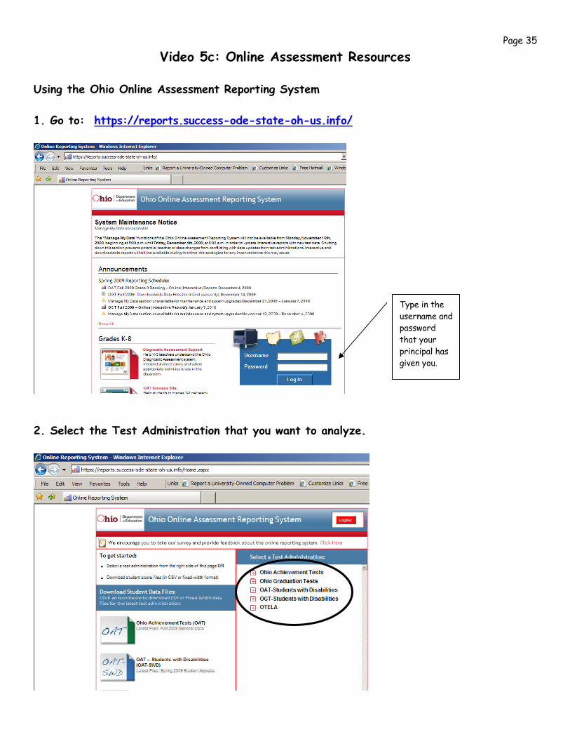
Video 5c: Online Assessment Resources

Using the Ohio Online Assessment Reporting System 1. Go to: https://reports.success-ode-state-oh-us.info/

2. Select the Test Administration that you want to analyze.

Type in the username and password that your principal has given you.

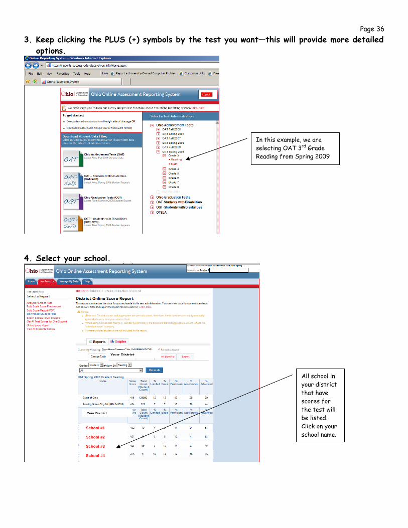
Page 36 3. Keep clicking the PLUS (+) symbols by the test you want—this will provide more detailed

options.

4. Select your school.

In this example, we are selecting OAT 3rd Grade Reading from Spring 2009

Your District

School #1 School #2 School #3 School #4

Your District

All school in your district that have scores for the test will be listed. Click on your school name.

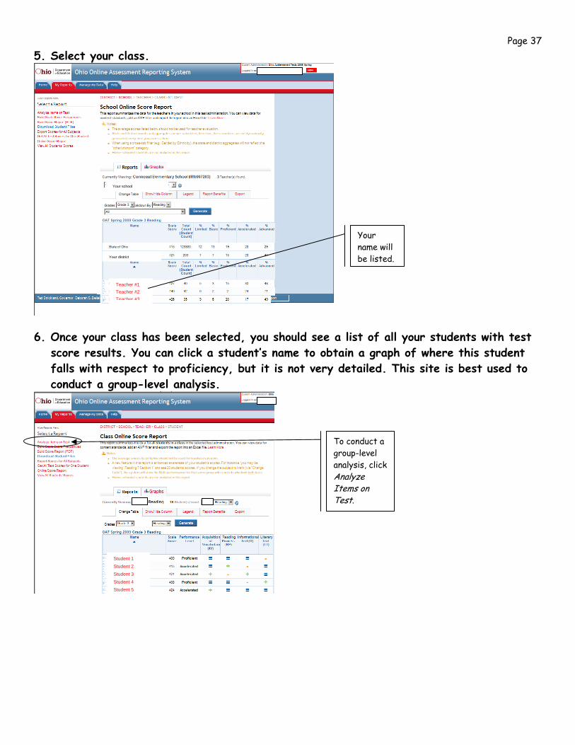
Page 37 5. Select your class.

6. Once your class has been selected, you should see a list of all your students with test

score results. You can click a student’s name to obtain a graph of where this student falls with respect to proficiency, but it is not very detailed. This site is best used to conduct a group-level analysis.

Your school

Your district

Teacher #1 Teacher #2 Teacher #3

Your name will be listed.

Student 1 Student 2 Student 3 Student 4 Student 5

To conduct a group-level analysis, click Analyze Items on Test.

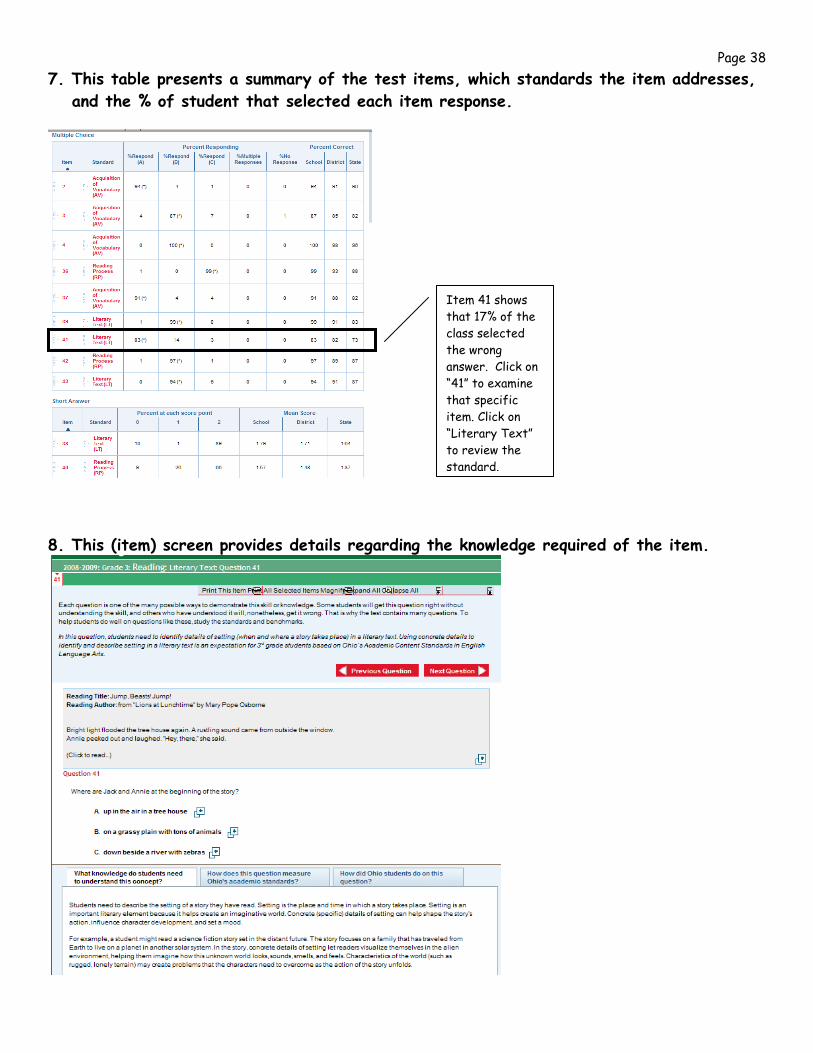
Page 38 7. This table presents a summary of the test items, which standards the item addresses,

and the % of student that selected each item response.

8. This (item) screen provides details regarding the knowledge required of the item.

Item 41 shows that 17% of the class selected the wrong answer. Click on “41” to examine that specific item. Click on “Literary Text” to review the standard.

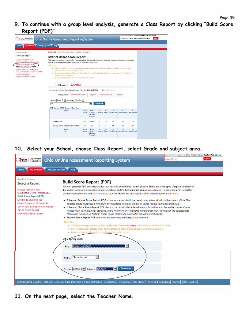
Page 39 9. To continue with a group level analysis, generate a Class Report by clicking “Build Score

Report (PDF)”

10. Select your School, choose Class Report, select Grade and subject area.

11. On the next page, select the Teacher Name.

Page 40

Week 7

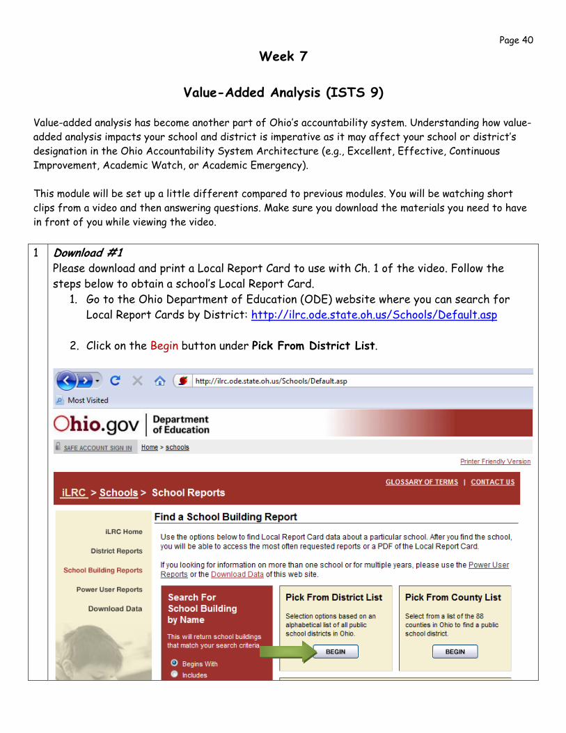
Value-Added Analysis (ISTS 9) Value-added analysis has become another part of Ohio’s accountability system. Understanding how value-added analysis impacts your school and district is imperative as it may affect your school or district’s designation in the Ohio Accountability System Architecture (e.g., Excellent, Effective, Continuous Improvement, Academic Watch, or Academic Emergency). This module will be set up a little different compared to previous modules. You will be watching short clips from a video and then answering questions. Make sure you download the materials you need to have in front of you while viewing the video. 1 Download #1

Please download and print a Local Report Card to use with Ch. 1 of the video. Follow the steps below to obtain a school’s Local Report Card.

1. Go to the Ohio Department of Education (ODE) website where you can search for Local Report Cards by District: http://ilrc.ode.state.oh.us/Schools/Default.asp

2. Click on the Begin button under Pick From District List.

Page 41

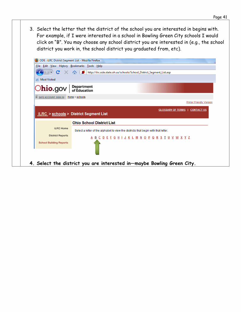
3. Select the letter that the district of the school you are interested in begins with. For example, if I were interested in a school in Bowling Green City schools I would click on “B”. You may choose any school district you are interested in (e.g., the school district you work in, the school district you graduated from, etc).

4. Select the district you are interested in—maybe Bowling Green City.

Page 42

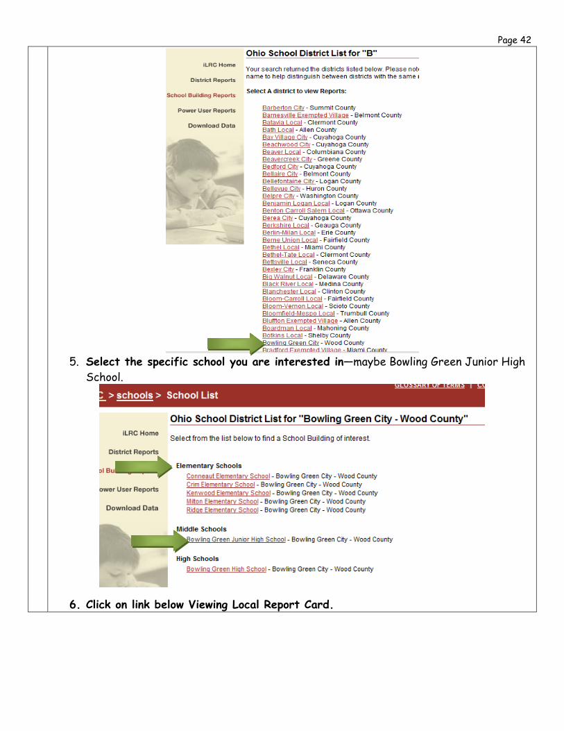
5. Select the specific school you are interested in—maybe Bowling Green Junior High

School.

6. Click on link below Viewing Local Report Card.

Page 43

7. Print the Local Report Card which will look similar to this:

2 Download #2

1. Go to: http://portal.battelleforkids.org/Ohio/Value_Added_and_Accountability/Accountability_toolkit.html?sflang=en

2. Click on Ohio Accountability System Architecture Chart and print chart for use with Ch. 3 of video.

Page 44

Page 45

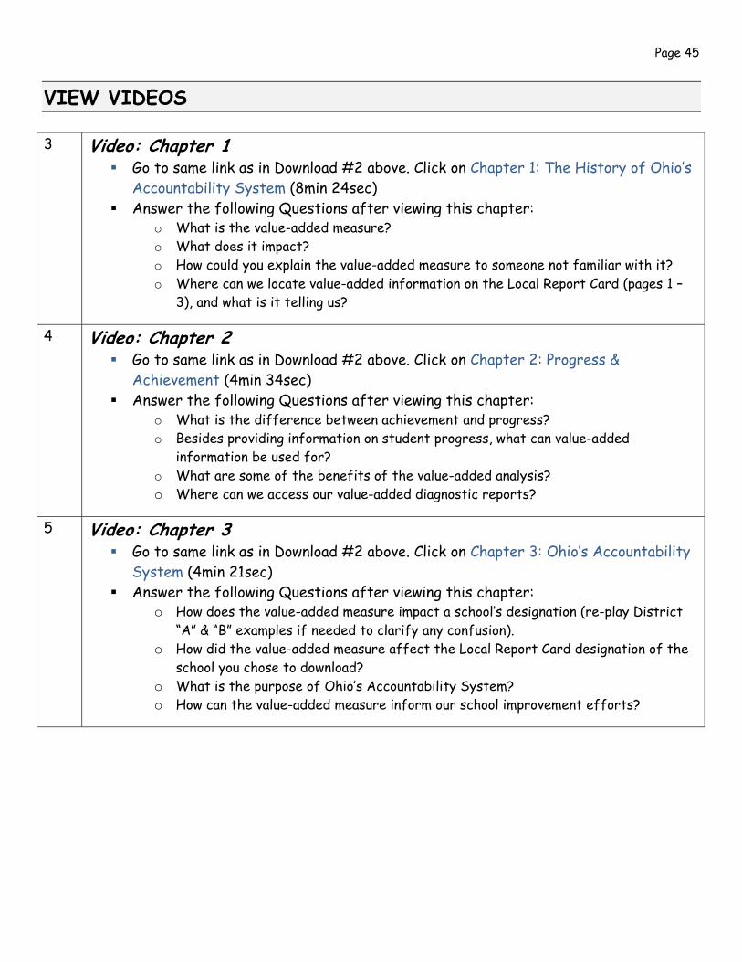
VIEW VIDEOS 3 Video: Chapter 1

Go to same link as in Download #2 above. Click on Chapter 1: The History of Ohio’s Accountability System (8min 24sec)

Answer the following Questions after viewing this chapter: o What is the value-added measure? o What does it impact? o How could you explain the value-added measure to someone not familiar with it? o Where can we locate value-added information on the Local Report Card (pages 1 –

3), and what is it telling us?

4 Video: Chapter 2 Go to same link as in Download #2 above. Click on Chapter 2: Progress &

Achievement (4min 34sec) Answer the following Questions after viewing this chapter:

o What is the difference between achievement and progress? o Besides providing information on student progress, what can value-added

information be used for? o What are some of the benefits of the value-added analysis? o Where can we access our value-added diagnostic reports?

5 Video: Chapter 3 Go to same link as in Download #2 above. Click on Chapter 3: Ohio’s Accountability

System (4min 21sec) Answer the following Questions after viewing this chapter:

o How does the value-added measure impact a school’s designation (re-play District “A” & “B” examples if needed to clarify any confusion).

o How did the value-added measure affect the Local Report Card designation of the school you chose to download?

o What is the purpose of Ohio’s Accountability System? o How can the value-added measure inform our school improvement efforts?

Page 46

Week 9

Video #7: Introduction to Inferential Statistics

Video #7a: The Basics of Inferential Statistics Population—the entire group of individuals that the researcher WISHES to study.

Sample—a set of individuals selected from population, intended to represent the population

Parameter—value that describes the population

Statistic—value that describes the sample Two major types of statistical methods • descriptive stats—summarize, organize and simplify data (e.g., mean, standard deviation, tables, graphs,

distributions) • data • raw score

• inferential stats—techniques that allow us to study samples and make generalizations about the population from which they were selected (e.g., t test, ANOVA, correlation)

• sampling error—amount of error between the sample statistic and the population parameter (degree to which the sample differs from the population)

• random sampling—used to minimize error between sample and population Inferential statistics also allow us to study relationships between/among variables that the sample holds. • variable—characteristic/condition that differs among individuals (gender, height, test scores, IQ)

• construct—hypothetical concepts/theory to organize observations • operational definition—defines a construct in terms of how it is measured

Types of Variables • categorical variable (discrete)—consists of separate categories (e.g., gender, religion, classification of

personality) • quantitative variable (continuous)—can be divided into an infinite number of fractional parts (e.g., height, time,

age) • independent variable—usually a treatment that has been manipulated (control group versus experimental

group), usually categorical • dependent variable—usually the effect, usually quantitative • confounding variable—an uncontrolled variable that creates a difference between the control and experimental

groups Variables determine type of relationship being studied

• mutual • causal

• Groups must be compared to examine cause and effect groups are created by a categorical variable

Page 47

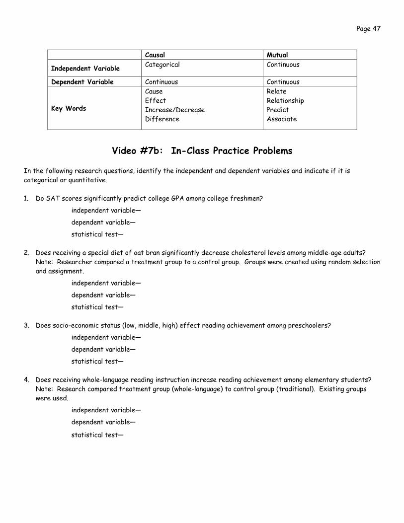
Video #7b: In-Class Practice Problems

In the following research questions, identify the independent and dependent variables and indicate if it is categorical or quantitative. 1. Do SAT scores significantly predict college GPA among college freshmen?

independent variable—

dependent variable—

statistical test— 2. Does receiving a special diet of oat bran significantly decrease cholesterol levels among middle-age adults?

Note: Researcher compared a treatment group to a control group. Groups were created using random selection and assignment.



statistical test— 3. Does socio-economic status (low, middle, high) effect reading achievement among preschoolers?



statistical test— 4. Does receiving whole-language reading instruction increase reading achievement among elementary students?

Note: Research compared treatment group (whole-language) to control group (traditional). Existing groups were used.



statistical test—

Causal Mutual

Independent Variable Categorical Continuous

Dependent Variable Continuous Continuous

Key Words

Cause Effect Increase/Decrease Difference

Relate Relationship Predict Associate

Page 48

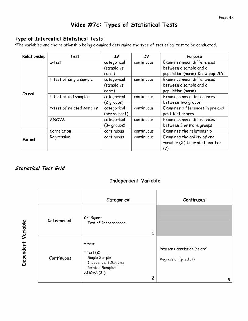
Video #7c: Types of Statistical Tests Type of Inferential Statistical Tests •The variables and the relationship being examined determine the type of statistical test to be conducted.

Relationship Test IV DV Purpose z-test categorical

(sample vs norm)

continuous Examines mean differences between a sample and a population (norm). Know pop. SD.

t-test of single sample categorical (sample vs norm)

continuous Examines mean differences between a sample and a population (norm)

t-test of ind samples categorical (2 groups)

continuous Examines mean differences between two groups

t-test of related samples categorical (pre vs post)

continuous Examines differences in pre and post test scores

Causal

ANOVA categorical (3+ groups)

continuous Examines mean differences between 3 or more groups

Correlation continuous continuous Examines the relationship

Mutual Regression continuous continuous Examines the ability of one variable (X) to predict another (Y)

Statistical Test Grid

Independent Variable

Categorical

Continuous

Categorical

Chi Square Test of Independence

1

Continuous

z test

t test (2) Single Sample Independent Samples Related Samples ANOVA (3+)

2

Pearson Correlation (relate) Regression (predict)

3

Dep

ende

nt V

ariable

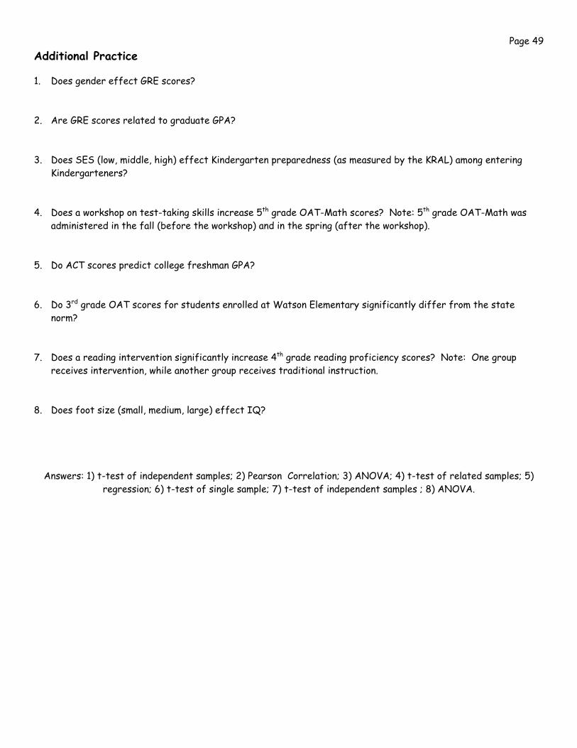
Page 49 Additional Practice 1. Does gender effect GRE scores? 2. Are GRE scores related to graduate GPA? 3. Does SES (low, middle, high) effect Kindergarten preparedness (as measured by the KRAL) among entering

Kindergarteners? 4. Does a workshop on test-taking skills increase 5th grade OAT-Math scores? Note: 5th grade OAT-Math was

administered in the fall (before the workshop) and in the spring (after the workshop). 5. Do ACT scores predict college freshman GPA? 6. Do 3rd grade OAT scores for students enrolled at Watson Elementary significantly differ from the state

norm? 7. Does a reading intervention significantly increase 4th grade reading proficiency scores? Note: One group

receives intervention, while another group receives traditional instruction. 8. Does foot size (small, medium, large) effect IQ?

Answers: 1) t-test of independent samples; 2) Pearson Correlation; 3) ANOVA; 4) t-test of related samples; 5) regression; 6) t-test of single sample; 7) t-test of independent samples ; 8) ANOVA.

Page 50

Video #7d: Distribution of Sample Means

Studying Samples With statistics, we are usually trying to make conclusions/inferences about the population from the studied sample.

• Consequently, we want to compare the sample to the population of similar samples. But in doing so, two issues arise:

• How do we know is a sample is representative of the population when every sample is different?

• How can we transform a population distribution of individuals to a population distribution of sample means?

• Every sample is different from the population, this is known as sampling error, or the

discrepancy/error between the sample and the population. • Random sampling is used to minimize sampling error, which can occur randomly

If we were to take a population distribution of individuals. . .

• randomly group individuals into similar sized samples • then calculated the means of these samples and placed them into a frequency distribution • a normal curve would form—this distribution is known as the distribution of sample means. • any distribution that is of sample statistics and NOT individual scores is referred to as a

sampling distribution. Characteristics of the distribution of sample means • will approach a normal distribution as sample size increases (a sample size greater than 30 is

considered normal) • the mean of the distribution of sample means is equal to the population mean of individuals and is also

known as the expected value of M. • standard deviation of this new distribution is called the standard error of M. • standard error (σx)—measures the standard distance between the sample mean (M) and the

population mean (μ); indicates how good an estimate M will be for μ.

• standard error (σx) = σ n

• as sample size increases, the standard error will decrease-----> which means that the samples are more representative of the population

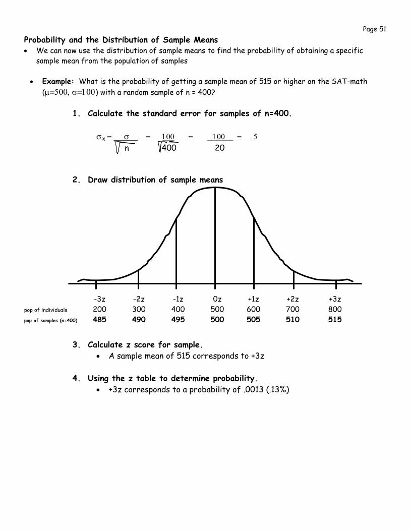
Page 51 Probability and the Distribution of Sample Means • We can now use the distribution of sample means to find the probability of obtaining a specific

sample mean from the population of samples

• Example: What is the probability of getting a sample mean of 515 or higher on the SAT-math (μ=500, σ=100) with a random sample of n = 400?

1. Calculate the standard error for samples of n=400.

σx = σ = 100 = 100 = 5 n 400 20

2. Draw distribution of sample means

-3z -2z -1z 0z +1z +2z +3z pop of individuals 200 300 400 500 600 700 800 pop of samples (n=400) 485 490 495 500 505 510 515

3. Calculate z score for sample. • A sample mean of 515 corresponds to +3z

4. Using the z table to determine probability.

• +3z corresponds to a probability of .0013 (.13%)

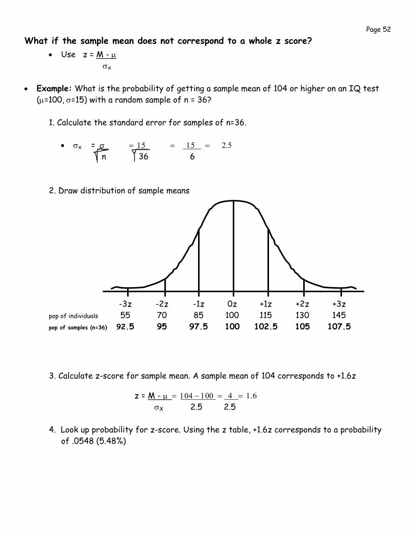
Page 52 What if the sample mean does not correspond to a whole z score?

• Use z = M - μ σx

• Example: What is the probability of getting a sample mean of 104 or higher on an IQ test (μ=100, σ=15) with a random sample of n = 36?

1. Calculate the standard error for samples of n=36.

• σx = σ = 15 = 15 = 2.5 n 36 6

2. Draw distribution of sample means

-3z -2z -1z 0z +1z +2z +3z pop of individuals 55 70 85 100 115 130 145 pop of samples (n=36) 92.5 95 97.5 100 102.5 105 107.5

3. Calculate z-score for sample mean. A sample mean of 104 corresponds to +1.6z

z = M - μ = 104 − 100 = 4 = 1.6 σX 2.5 2.5

4. Look up probability for z-score. Using the z table, +1.6z corresponds to a probability

of .0548 (5.48%)

Page 53

Video #7e: In-Class Practice Problems

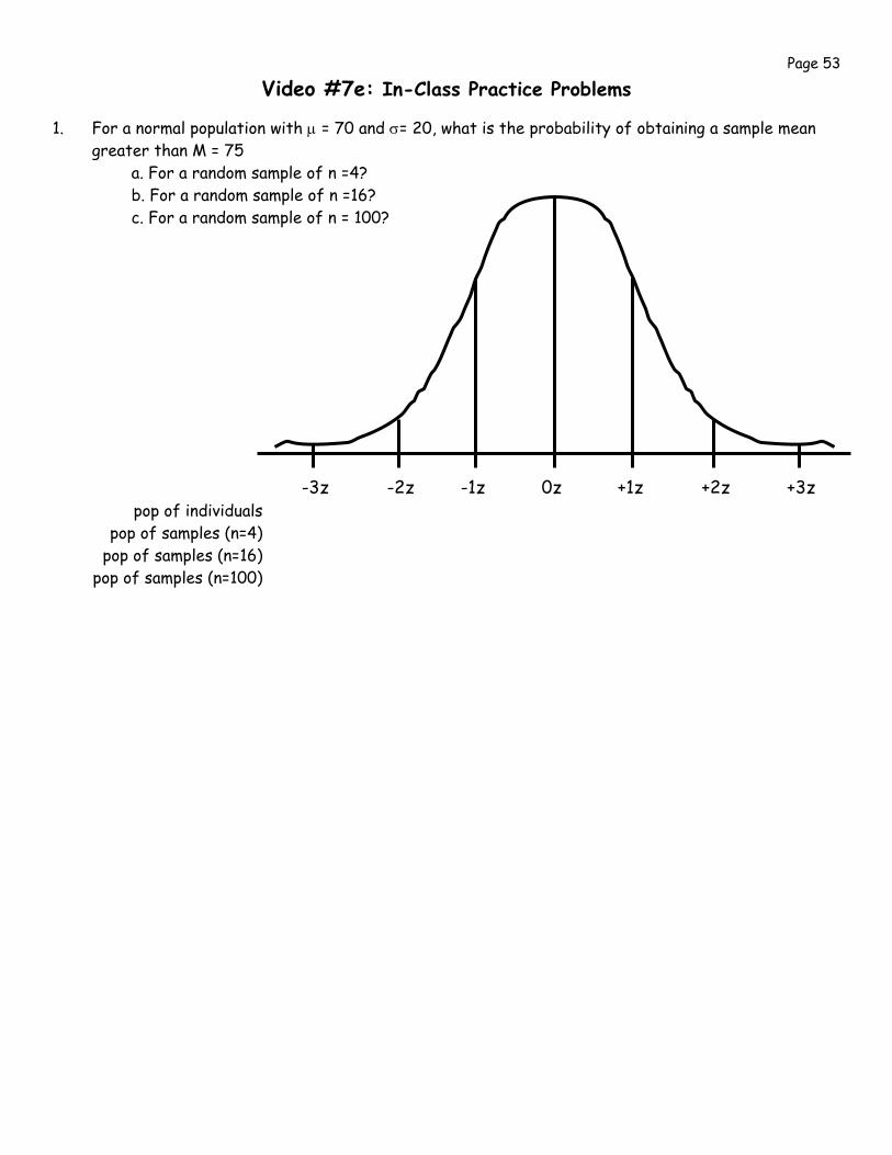
1. For a normal population with μ = 70 and σ= 20, what is the probability of obtaining a sample mean greater than M = 75

a. For a random sample of n =4? b. For a random sample of n =16? c. For a random sample of n = 100?

-3z -2z -1z 0z +1z +2z +3z pop of individuals pop of samples (n=4) pop of samples (n=16) pop of samples (n=100)

Page 54

Week 10

Video #8: Hypothesis Testing

Video #8a: Process of Hypothesis Testing Hypothesis Testing—using sample data to evaluate a hypothesis (prediction) about the population so conclusions/inferences can be made about the population from the sample

• We are testing a hypothesis to determine if the treatment has caused a significant change in the population

• the majority of sample means are in the middle of the distribution; so for a sample to be significantly different, it should be with the extreme means in the tails of the distribution, where the probability is very low

Steps in Hypothesis Testing

1. State the Hypotheses 2. Establish significance criteria 3. Collect and analyze data 4. Evaluate null hypothesis 5. Draw conclusion Step 1—Stating the Hypothesis

• hypotheses should be stated in terms of the population • like a research question, your hypothesis should include three parts: variables, relationship, and sample • two hypotheses must be developed—an alternative and a null

• alternative hypothesis—the actual prediction about the change or relationship that may occur in the population

• null hypothesis—statement that the treatment has no effect on the population

• hypotheses can also be directional or non-directional • non-directional—just a prediction of a change/effect

• Key words: effect, impact, difference, cause

• directional—a prediction of increase or decrease • Key words: increase, decrease, higher, lower, positive, negative

• Example: Suppose that local school district implemented an experimental program for science education.

After one year, 50 children in the special program obtained a mean score of M=63 on a national science achievement test (μ=60, σ=12). Did the program have an impact on the participants’ science achievement?

• alternative—The experimental science program will significantly effect science achievement scores

among program participants.

• null— The experimental science program will NOT significantly effect science achievement scores among program participants.

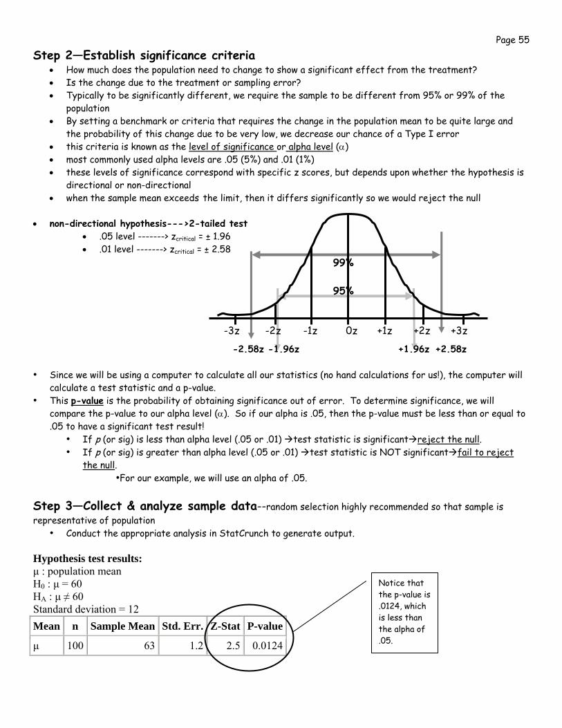
Page 55 Step 2—Establish significance criteria

• How much does the population need to change to show a significant effect from the treatment? • Is the change due to the treatment or sampling error? • Typically to be significantly different, we require the sample to be different from 95% or 99% of the

population • By setting a benchmark or criteria that requires the change in the population mean to be quite large and

the probability of this change due to be very low, we decrease our chance of a Type I error • this criteria is known as the level of significance or alpha level (α) • most commonly used alpha levels are .05 (5%) and .01 (1%) • these levels of significance correspond with specific z scores, but depends upon whether the hypothesis is

directional or non-directional • when the sample mean exceeds the limit, then it differs significantly so we would reject the null

• non-directional hypothesis--->2-tailed test • .05 level -------> zcritical = ± 1.96 • .01 level -------> zcritical = ± 2.58

99%

95%

-3z -2z -1z 0z +1z +2z +3z

-2.58z -1.96z +1.96z +2.58z

• Since we will be using a computer to calculate all our statistics (no hand calculations for us!), the computer will calculate a test statistic and a p-value.

• This p-value is the probability of obtaining significance out of error. To determine significance, we will compare the p-value to our alpha level (α). So if our alpha is .05, then the p-value must be less than or equal to .05 to have a significant test result!

• If p (or sig) is less than alpha level (.05 or .01) test statistic is significant reject the null. • If p (or sig) is greater than alpha level (.05 or .01) test statistic is NOT significant fail to reject

the null. •For our example, we will use an alpha of .05.

Step 3—Collect & analyze sample data--random selection highly recommended so that sample is representative of population

• Conduct the appropriate analysis in StatCrunch to generate output. Hypothesis test results: μ : population mean H0 : μ = 60 HA : μ ≠ 60 Standard deviation = 12

Mean n Sample Mean Std. Err. Z-Stat P-value

μ 100 63 1.2 2.5 0.0124

Notice that the p-value is .0124, which is less than the alpha of .05.

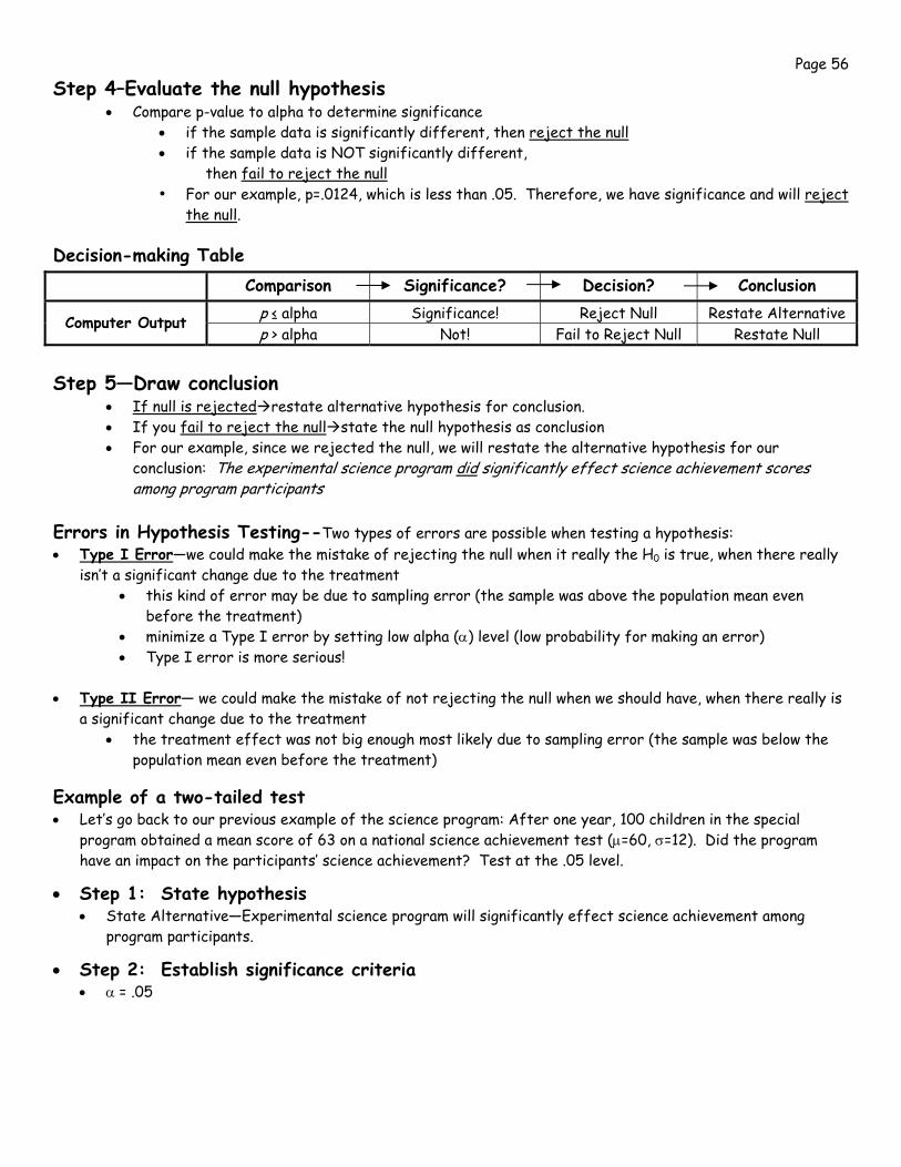
Page 56 Step 4–Evaluate the null hypothesis

• Compare p-value to alpha to determine significance • if the sample data is significantly different, then reject the null • if the sample data is NOT significantly different,

then fail to reject the null • For our example, p=.0124, which is less than .05. Therefore, we have significance and will reject

the null.

Decision-making Table Comparison Significance? Decision? Conclusion

p ≤ alpha Significance! Reject Null Restate Alternative Computer Output p > alpha Not! Fail to Reject Null Restate Null

Step 5—Draw conclusion

• If null is rejected restate alternative hypothesis for conclusion. • If you fail to reject the null state the null hypothesis as conclusion • For our example, since we rejected the null, we will restate the alternative hypothesis for our

conclusion: The experimental science program did significantly effect science achievement scores among program participants

Errors in Hypothesis Testing--Two types of errors are possible when testing a hypothesis: • Type I Error—we could make the mistake of rejecting the null when it really the H0 is true, when there really

isn’t a significant change due to the treatment • this kind of error may be due to sampling error (the sample was above the population mean even

before the treatment) • minimize a Type I error by setting low alpha (α) level (low probability for making an error) • Type I error is more serious!

• Type II Error— we could make the mistake of not rejecting the null when we should have, when there really is

a significant change due to the treatment • the treatment effect was not big enough most likely due to sampling error (the sample was below the

population mean even before the treatment)

Example of a two-tailed test • Let’s go back to our previous example of the science program: After one year, 100 children in the special

program obtained a mean score of 63 on a national science achievement test (μ=60, σ=12). Did the program have an impact on the participants’ science achievement? Test at the .05 level.

• Step 1: State hypothesis • State Alternative—Experimental science program will significantly effect science achievement among

program participants.

• Step 2: Establish significance criteria • α = .05

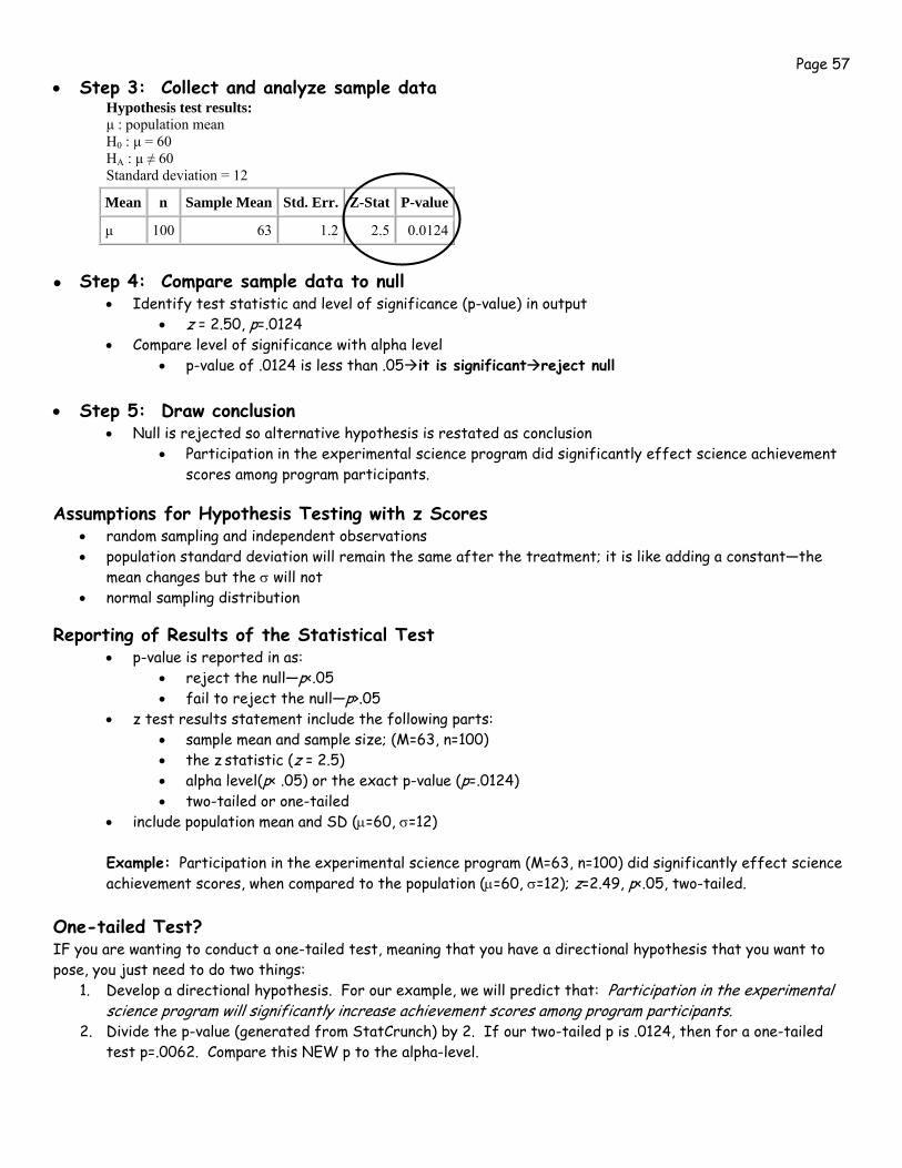
Page 57 • Step 3: Collect and analyze sample data

Hypothesis test results: μ : population mean H0 : μ = 60 HA : μ ≠ 60 Standard deviation = 12

Step 4: Compare sample data to null • Identify test statistic and level of significance (p-value) in output

• z = 2.50, p=.0124 • Compare level of significance with alpha level

• p-value of .0124 is less than .05 it is significant reject null • Step 5: Draw conclusion

• Null is rejected so alternative hypothesis is restated as conclusion • Participation in the experimental science program did significantly effect science achievement

scores among program participants.

Assumptions for Hypothesis Testing with z Scores • random sampling and independent observations • population standard deviation will remain the same after the treatment; it is like adding a constant—the

mean changes but the σ will not • normal sampling distribution

Reporting of Results of the Statistical Test • p-value is reported in as:

• reject the null—p<.05 • fail to reject the null—p>.05

• z test results statement include the following parts: • sample mean and sample size; (M=63, n=100) • the z statistic (z = 2.5) • alpha level(p< .05) or the exact p-value (p=.0124) • two-tailed or one-tailed

• include population mean and SD (μ=60, σ=12)

Example: Participation in the experimental science program (M=63, n=100) did significantly effect science achievement scores, when compared to the population (μ=60, σ=12); z=2.49, p<.05, two-tailed.

One-tailed Test? IF you are wanting to conduct a one-tailed test, meaning that you have a directional hypothesis that you want to pose, you just need to do two things:

1. Develop a directional hypothesis. For our example, we will predict that: Participation in the experimental science program will significantly increase achievement scores among program participants.

2. Divide the p-value (generated from StatCrunch) by 2. If our two-tailed p is .0124, then for a one-tailed test p=.0062. Compare this NEW p to the alpha-level.


μ 100 63 1.2 2.5 0.0124

Page 58

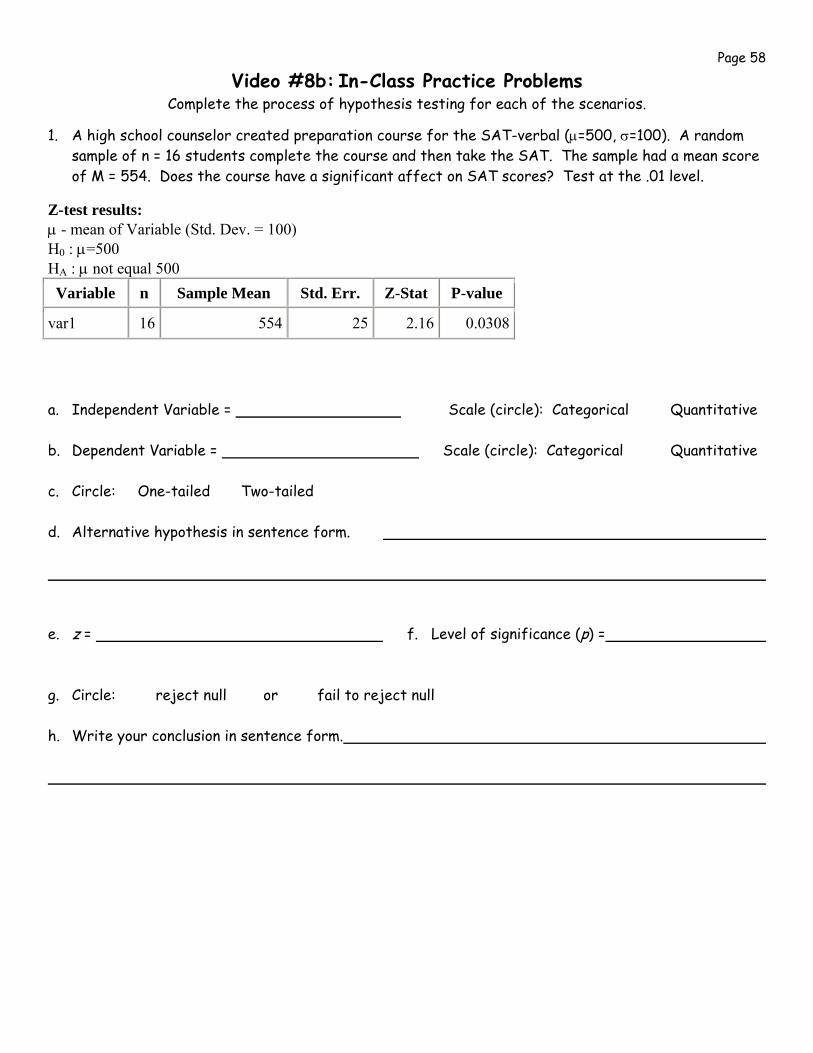
Video #8b: In-Class Practice Problems Complete the process of hypothesis testing for each of the scenarios.

1. A high school counselor created preparation course for the SAT-verbal (μ=500, σ=100). A random sample of n = 16 students complete the course and then take the SAT. The sample had a mean score of M = 554. Does the course have a significant affect on SAT scores? Test at the .01 level.

Z-test results: μ - mean of Variable (Std. Dev. = 100) H0 : μ=500 HA : μ not equal 500

a. Independent Variable = Scale (circle): Categorical Quantitative b. Dependent Variable = Scale (circle): Categorical Quantitative c. Circle: One-tailed Two-tailed d. Alternative hypothesis in sentence form. e. z = f. Level of significance (p) = g. Circle: reject null or fail to reject null h. Write your conclusion in sentence form.

Variable n Sample Mean Std. Err. Z-Stat P-value

var1 16 554 25 2.16 0.0308

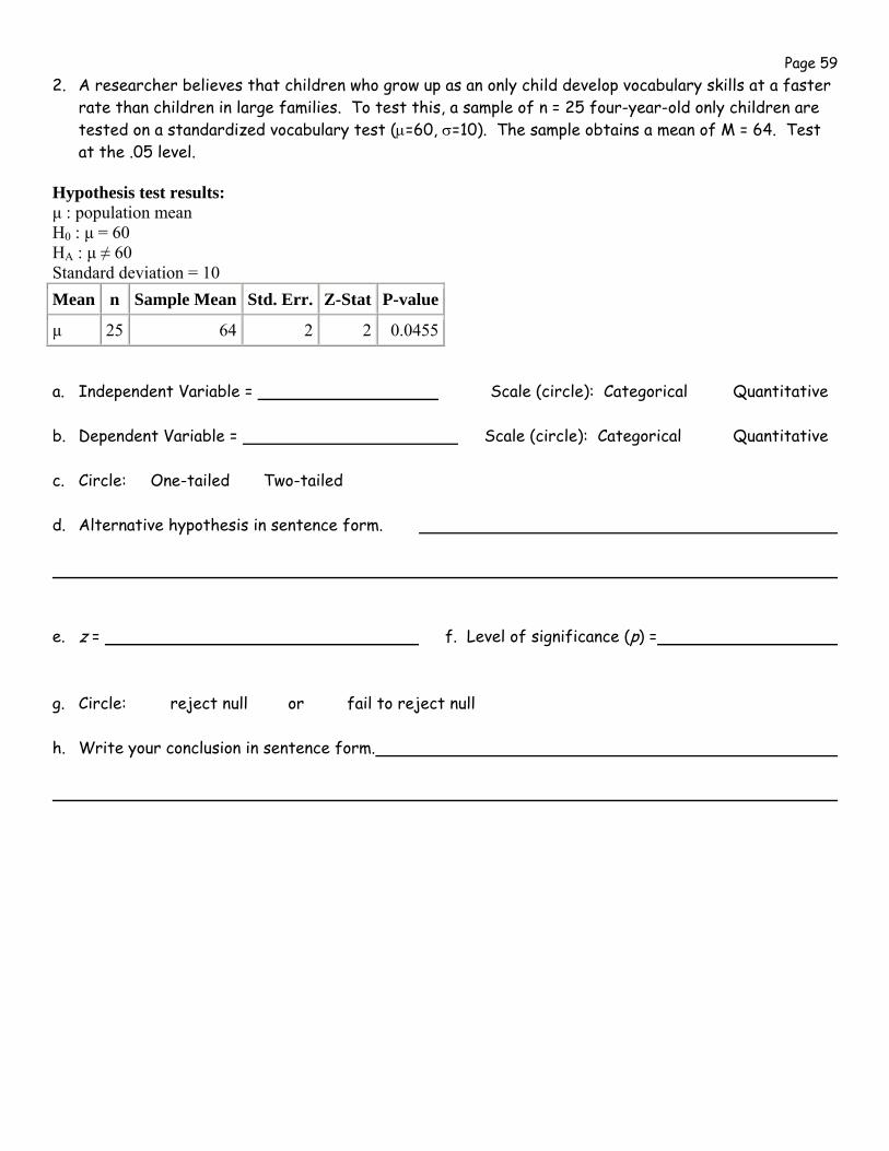
Page 59 2. A researcher believes that children who grow up as an only child develop vocabulary skills at a faster

rate than children in large families. To test this, a sample of n = 25 four-year-old only children are tested on a standardized vocabulary test (μ=60, σ=10). The sample obtains a mean of M = 64. Test at the .05 level.

Hypothesis test results: μ : population mean H0 : μ = 60 HA : μ ≠ 60 Standard deviation = 10

a. Independent Variable = Scale (circle): Categorical Quantitative b. Dependent Variable = Scale (circle): Categorical Quantitative c. Circle: One-tailed Two-tailed d. Alternative hypothesis in sentence form. e. z = f. Level of significance (p) = g. Circle: reject null or fail to reject null h. Write your conclusion in sentence form.


μ 25 64 2 2 0.0455

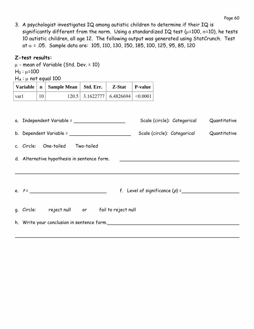
Page 60 3. A psychologist investigates IQ among autistic children to determine if their IQ is

significantly different from the norm. Using a standardized IQ test (μ=100, σ=10), he tests 10 autistic children, all age 12. The following output was generated using StatCrunch. Test at α = .05. Sample data are: 105, 110, 130, 150, 185, 100, 125, 95, 85, 120

Z-test results: μ - mean of Variable (Std. Dev. = 10) H0 : μ=100 HA : μ not equal 100

a. Independent Variable = Scale (circle): Categorical Quantitative b. Dependent Variable = Scale (circle): Categorical Quantitative c. Circle: One-tailed Two-tailed d. Alternative hypothesis in sentence form. e. t = f. Level of significance (p) = g. Circle: reject null or fail to reject null h. Write your conclusion in sentence form.

Variable n Sample Mean Std. Err. Z-Stat P-value

var1 10 120.5 3.1622777 6.4826694 <0.0001

Page 61

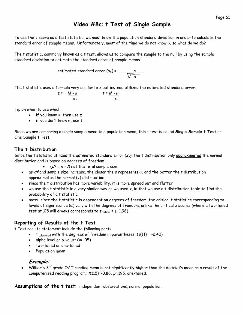
Video #8c: t Test of Single Sample To use the z score as a test statistic, we must know the population standard deviation in order to calculate the standard error of sample means. Unfortunately, most of the time we do not know σ, so what do we do? The t statistic, commonly known as a t test, allows us to compare the sample to the null by using the sample standard deviation to estimate the standard error of sample means. estimated standard error (sX) = s n The t statistic uses a formula very similar to z but instead utilizes the estimated standard error.

z = M - μ t = M - μ σX sX Tip on when to use which:

• if you know σ, then use z • if you don’t know σ, use t

Since we are comparing a single sample mean to a population mean, this t test is called Single Sample t Test or One Sample t Test. The t Distribution Since the t statistic utilizes the estimated standard error (sX), the t distribution only approximates the normal distribution and is based on degrees of freedom

• (df = n - 1) not the total sample size. • as df and sample size increase, the closer the s represents σ, and the better the t distribution

approximates the normal (z) distribution • since the t distribution has more variability, it is more spread out and flatter • we use the t statistic in a very similar way as we used z, in that we use a t distribution table to find the

probability of a t statistic • note: since the t statistic is dependent on degrees of freedom, the critical t statistics corresponding to

levels of significance (α) vary with the degrees of freedom, unlike the critical z scores (where a two-tailed test at .05 will always corresponds to zcritical = ± 1.96)

Reporting of Results of the t Test t Test results statement include the following parts:

• t calculated with the degrees of freedom in parentheses; (t(11) = -2.40) • alpha level or p-value; (p< .05) • two-tailed or one-tailed • Population mean

Example: • William’s 3rd grade OAT reading mean is not significantly higher than the district’s mean as a result of the

computerized reading program; t(115)=-0.86, p=.195, one-tailed.

Assumptions of the t test: independent observations, normal population

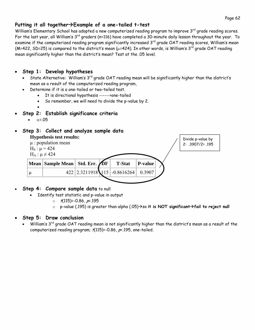
Page 62 Putting it all together Example of a one-tailed t-test William’s Elementary School has adopted a new computerized reading program to improve 3rd grade reading scores. For the last year, all William’s 3rd graders (n=116) have completed a 30-minute daily lesson throughout the year. To examine if the computerized reading program significantly increased 3rd grade OAT reading scores, William’s mean (M=422, SD=25) is compared to the district’s mean (μ=424). In other words, is William’s 3rd grade OAT reading mean significantly higher than the district’s mean? Test at the .05 level.

• Step 1: Develop hypotheses • State Alternative: William’s 3rd grade OAT reading mean will be significantly higher than the district’s

mean as a result of the computerized reading program, • Determine if it is a one-tailed or two-tailed test.

• It is directional hypothesis ------>one-tailed • So remember, we will need to divide the p-value by 2. •

• Step 2: Establish significance criteria • α=.05

• Step 3: Collect and analyze sample data Hypothesis test results: μ : population mean H0 : μ = 424 HA : μ ≠ 424

• Step 4: Compare sample data to null

• Identify test statistic and p-value in output o t(115)=-0.86, p=.195 o p-value (.195) is greater than alpha (.05) so it is NOT significant fail to reject null

• Step 5: Draw conclusion • William’s 3rd grade OAT reading mean is not significantly higher than the district’s mean as a result of the

computerized reading program; t(115)=-0.86, p=.195, one-tailed.

Mean Sample Mean Std. Err. DF T-Stat P-value

μ 422 2.3211918 115 -0.8616264 0.3907

Divide p-value by 2: .3907/2= .195

Page 63

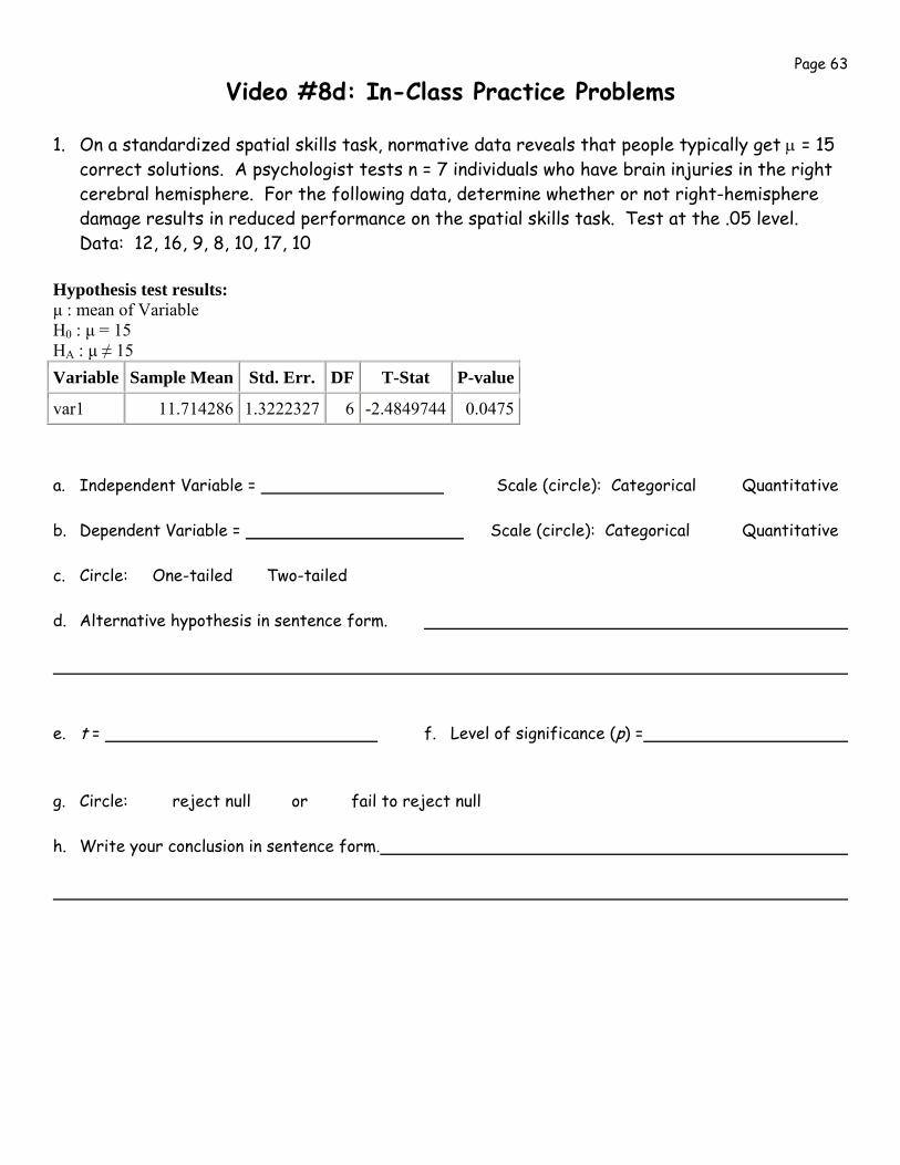
Video #8d: In-Class Practice Problems 1. On a standardized spatial skills task, normative data reveals that people typically get μ = 15

correct solutions. A psychologist tests n = 7 individuals who have brain injuries in the right cerebral hemisphere. For the following data, determine whether or not right-hemisphere damage results in reduced performance on the spatial skills task. Test at the .05 level. Data: 12, 16, 9, 8, 10, 17, 10

Hypothesis test results: μ : mean of Variable H0 : μ = 15 HA : μ ≠ 15


Variable Sample Mean Std. Err. DF T-Stat P-value

var1 11.714286 1.3222327 6 -2.4849744 0.0475

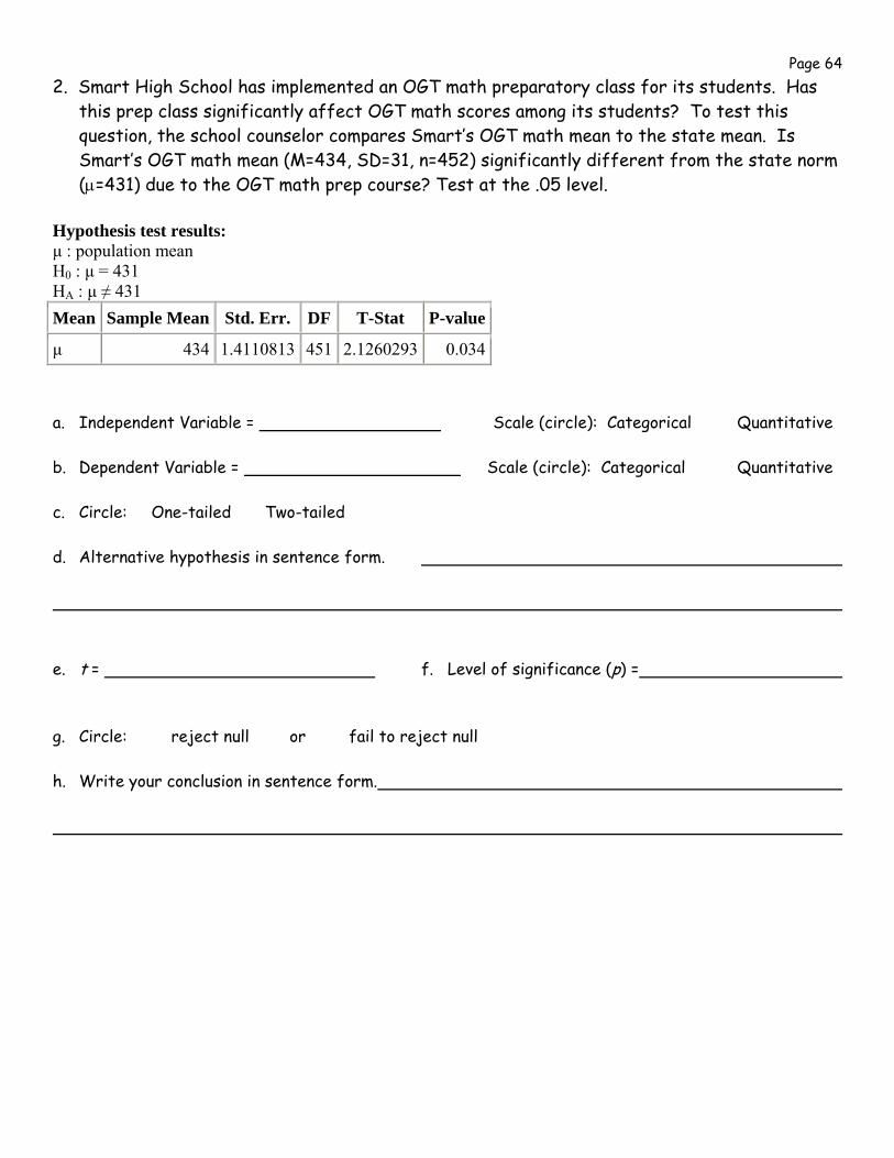
Page 64 2. Smart High School has implemented an OGT math preparatory class for its students. Has

this prep class significantly affect OGT math scores among its students? To test this question, the school counselor compares Smart’s OGT math mean to the state mean. Is Smart’s OGT math mean (M=434, SD=31, n=452) significantly different from the state norm (μ=431) due to the OGT math prep course? Test at the .05 level.

Hypothesis test results: μ : population mean H0 : μ = 431 HA : μ ≠ 431



μ 434 1.4110813 451 2.1260293 0.034

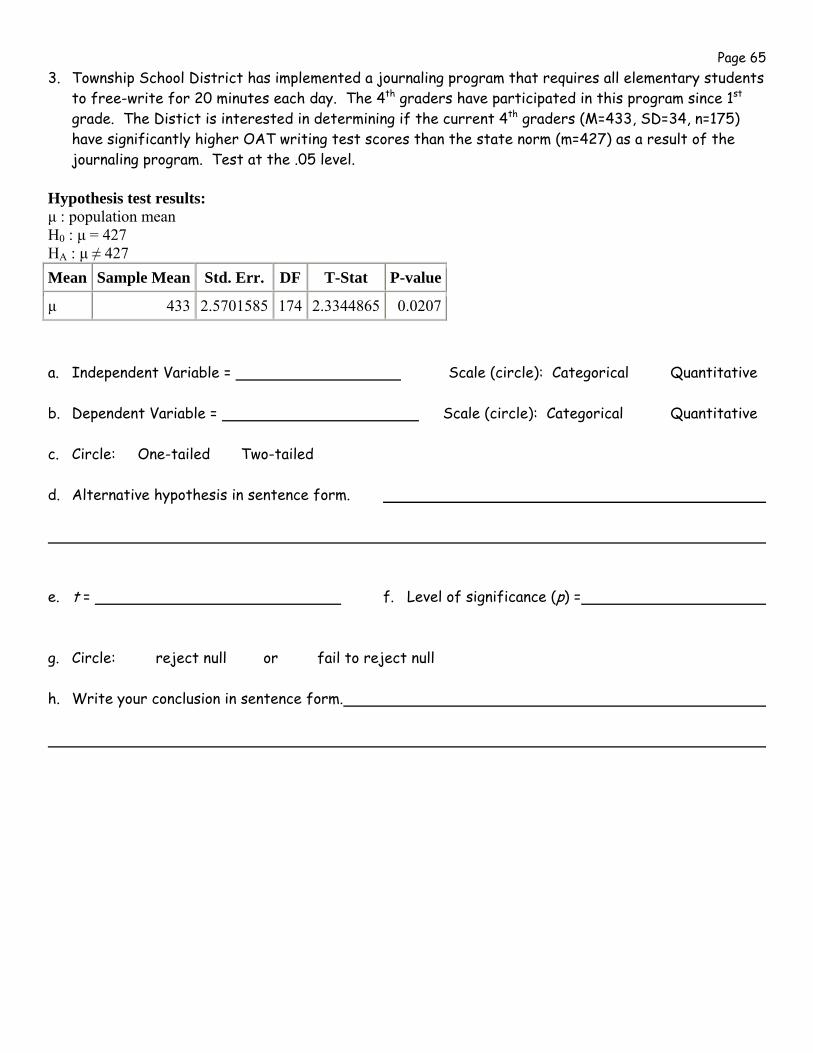
Page 65 3. Township School District has implemented a journaling program that requires all elementary students

to free-write for 20 minutes each day. The 4th graders have participated in this program since 1st grade. The Distict is interested in determining if the current 4th graders (M=433, SD=34, n=175) have significantly higher OAT writing test scores than the state norm (m=427) as a result of the journaling program. Test at the .05 level.

Hypothesis test results: μ : population mean H0 : μ = 427 HA : μ ≠ 427



μ 433 2.5701585 174 2.3344865 0.0207

Page 66

Week 11

Video #9: t Tests of Independent Samples & Related Samples

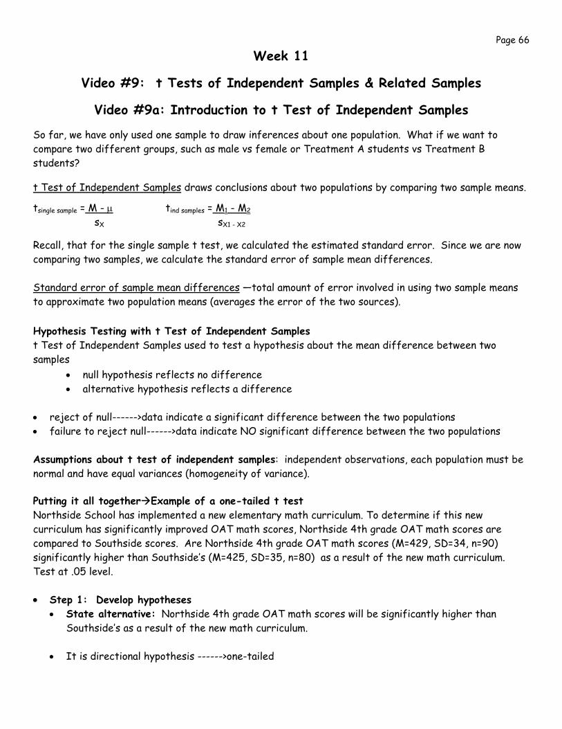
Video #9a: Introduction to t Test of Independent Samples

So far, we have only used one sample to draw inferences about one population. What if we want to compare two different groups, such as male vs female or Treatment A students vs Treatment B students?

t Test of Independent Samples draws conclusions about two populations by comparing two sample means.

tsingle sample = M - μ tind samples = M1 - M2 sX sX1 - X2

Recall, that for the single sample t test, we calculated the estimated standard error. Since we are now comparing two samples, we calculate the standard error of sample mean differences. Standard error of sample mean differences —total amount of error involved in using two sample means to approximate two population means (averages the error of the two sources). Hypothesis Testing with t Test of Independent Samples t Test of Independent Samples used to test a hypothesis about the mean difference between two samples

• null hypothesis reflects no difference • alternative hypothesis reflects a difference

• reject of null------>data indicate a significant difference between the two populations • failure to reject null------>data indicate NO significant difference between the two populations Assumptions about t test of independent samples: independent observations, each population must be normal and have equal variances (homogeneity of variance).

Putting it all together Example of a one-tailed t test Northside School has implemented a new elementary math curriculum. To determine if this new curriculum has significantly improved OAT math scores, Northside 4th grade OAT math scores are compared to Southside scores. Are Northside 4th grade OAT math scores (M=429, SD=34, n=90) significantly higher than Southside’s (M=425, SD=35, n=80) as a result of the new math curriculum. Test at .05 level. • Step 1: Develop hypotheses

• State alternative: Northside 4th grade OAT math scores will be significantly higher than Southside’s as a result of the new math curriculum.

• It is directional hypothesis ------>one-tailed

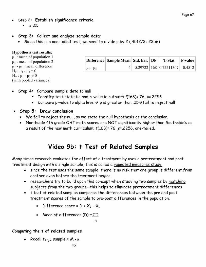
Page 67 • Step 2: Establish significance criteria

• α=.05

• Step 3: Collect and analyze sample data; • Since this is a one-tailed test, we need to divide p by 2 (.4512/2=.2256)

Hypothesis test results: μ1 : mean of population 1 μ2 : mean of population 2 μ1 - μ2 : mean difference H0 : μ1 - μ2 = 0 HA : μ1 - μ2 ≠ 0 (with pooled variances) • Step 4: Compare sample data to null

Identify test statistic and p-value in output t(168)=.76, p=.2256 • Compare p-value to alpha level p is greater than .05 fail to reject null

• Step 5: Draw conclusion • We fail to reject the null, so we state the null hypothesis as the conclusion. • Northside 4th grade OAT math scores are NOT significantly higher than Southside’s as

a result of the new math curriculum; t(168)=.76, p=.2256, one-tailed.

Video 9b: t Test of Related Samples Many times research evaluates the effect of a treatment by uses a pretreatment and post treatment design with a single sample, this is called a repeated measures study.

• since the test uses the same sample, there is no risk that one group is different from another even before the treatment begins.

• researchers try to build upon this concept when studying two samples by matching subjects from the two groups--this helps to eliminate pretreatment differences

• t test of related samples compares the differences between the pre and post treatment scores of the sample to pre-post differences in the population.

• Difference score = D = X2 - X1

• Mean of differences (D) = ΣD n Computing the t of related samples

• Recall tsingle sample = M - μ sX

Difference Sample Mean Std. Err. DF T-Stat P-value

μ1 - μ2 4 5.29722 168 0.75511307 0.4512

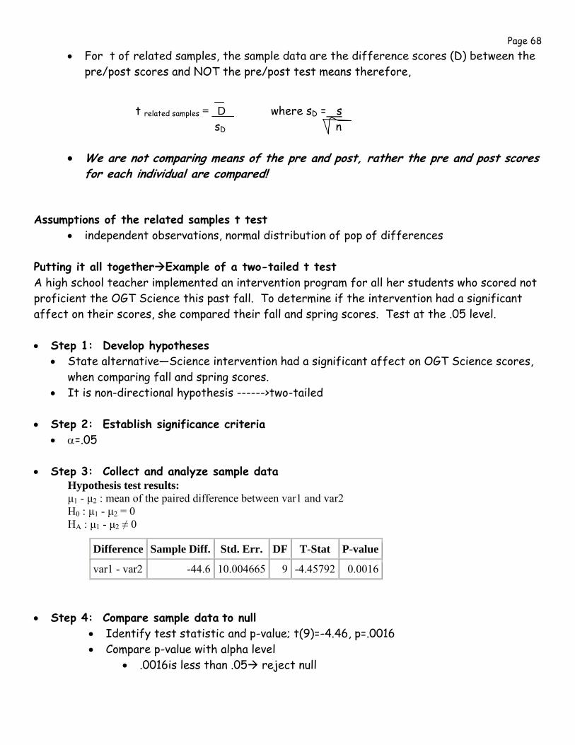
Page 68 • For t of related samples, the sample data are the difference scores (D) between the

pre/post scores and NOT the pre/post test means therefore,

t related samples = D where sD = s sD n

• We are not comparing means of the pre and post, rather the pre and post scores for each individual are compared!

Assumptions of the related samples t test

• independent observations, normal distribution of pop of differences Putting it all together Example of a two-tailed t test A high school teacher implemented an intervention program for all her students who scored not proficient the OGT Science this past fall. To determine if the intervention had a significant affect on their scores, she compared their fall and spring scores. Test at the .05 level. • Step 1: Develop hypotheses

• State alternative—Science intervention had a significant affect on OGT Science scores, when comparing fall and spring scores.

• It is non-directional hypothesis ------>two-tailed • Step 2: Establish significance criteria

• α=.05

• Step 3: Collect and analyze sample data Hypothesis test results: μ1 - μ2 : mean of the paired difference between var1 and var2 H0 : μ1 - μ2 = 0 HA : μ1 - μ2 ≠ 0

• Step 4: Compare sample data to null

• Identify test statistic and p-value; t(9)=-4.46, p=.0016 • Compare p-value with alpha level

• .0016is less than .05 reject null

Difference Sample Diff. Std. Err. DF T-Stat P-value

var1 - var2 -44.6 10.004665 9 -4.45792 0.0016

Page 69

• Step 5: Draw conclusion • Since we reject the null, we restate the alternative hypothesis as our conclusion:

• Science intervention had a significant affect on OGT Science scores, when comparing fall and spring scores; t(9)=-4.46, p=.0016, two-tailed.

Video#9c: In-Class Practice Problems

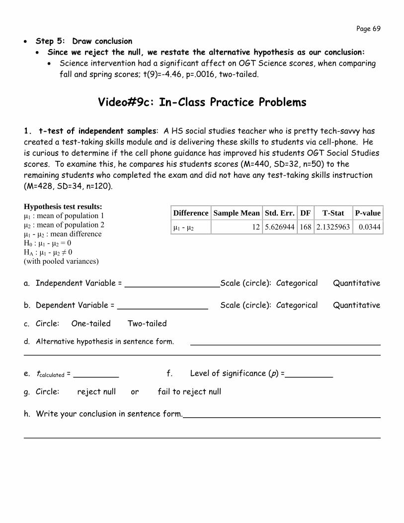
1. t-test of independent samples: A HS social studies teacher who is pretty tech-savvy has created a test-taking skills module and is delivering these skills to students via cell-phone. He is curious to determine if the cell phone guidance has improved his students OGT Social Studies scores. To examine this, he compares his students scores (M=440, SD=32, n=50) to the remaining students who completed the exam and did not have any test-taking skills instruction (M=428, SD=34, n=120). Hypothesis test results: μ1 : mean of population 1 μ2 : mean of population 2 μ1 - μ2 : mean difference H0 : μ1 - μ2 = 0 HA : μ1 - μ2 ≠ 0 (with pooled variances) a. Independent Variable = Scale (circle): Categorical Quantitative b. Dependent Variable = Scale (circle): Categorical Quantitative

c. Circle: One-tailed Two-tailed

d. Alternative hypothesis in sentence form. e. tcalculated = f. Level of significance (p) =

g. Circle: reject null or fail to reject null h. Write your conclusion in sentence form.


μ1 - μ2 12 5.626944 168 2.1325963 0.0344

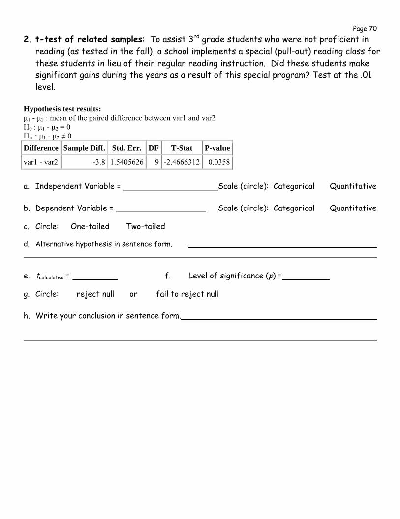
Page 70 2. t-test of related samples: To assist 3rd grade students who were not proficient in

reading (as tested in the fall), a school implements a special (pull-out) reading class for these students in lieu of their regular reading instruction. Did these students make significant gains during the years as a result of this special program? Test at the .01 level.

Hypothesis test results: μ1 - μ2 : mean of the paired difference between var1 and var2 H0 : μ1 - μ2 = 0 HA : μ1 - μ2 ≠ 0

a. Independent Variable = Scale (circle): Categorical Quantitative b. Dependent Variable = Scale (circle): Categorical Quantitative




Difference Sample Diff. Std. Err. DF T-Stat P-value

var1 - var2 -3.8 1.5405626 9 -2.4666312 0.0358

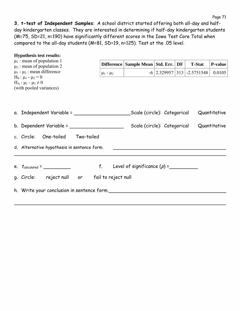
Page 71 3. t-test of Independent Samples: A school district started offering both all-day and half-day kindergarten classes. They are interested in determining if half-day kindergarten students (M=75, SD=21, n=190) have significantly different scores in the Iowa Test Core Total when compared to the all-day students (M=81, SD=19, n=125). Test at the .05 level. Hypothesis test results: μ1 : mean of population 1 μ2 : mean of population 2 μ1 - μ2 : mean difference H0 : μ1 - μ2 = 0 HA : μ1 - μ2 ≠ 0 (with pooled variances) a. Independent Variable = Scale (circle): Categorical Quantitative b. Dependent Variable = Scale (circle): Categorical Quantitative





μ1 - μ2 -6 2.329957 313 -2.5751548 0.0105

Page 72

Week 12

Video #10: Analysis of Variance

Video #10a: Introduction to Analysis of Variance Analysis of Variance (ANOVA) is a hypothesis testing procedure that evaluates mean differences between two or more treatments or groups; t test can only compare two groups. Single Factor Design—studies the effect that one factor (independent variable) has on the dependent variable. Note that although there is only one factor, this factor has more than two categories so that we are comparing two or more groups/treatments. Hypothesis Testing for ANOVA

• Null hypothesis states that there is no difference among the groups or treatments • Alternative hypothesis states that at least one mean is different from the others

ANOVA Test Statistic ANOVA creates a test statistic called an F-ratio that is similar to t statistic

• Recall that t = obtained difference between sample means = tsingle = X - μ difference expected by chance (error) sX

• F is similar to t, but since there are more than two means to compare, variance will be used to represent the differences between all the means being compared.

F = variance (differences ) between sample means variance (differences ) expected by chance (error)

• Like t, a large F value indicates the treatment effect (mean differences) that is unlikely due to chance.

• when the treatment had no effect so that the means are the same (H0 is true), the F-ratio will be close to 1.00

Distribution of F-ratios • Like t, F is also distributed • But the F distribution is not normal; it is positively skewed, the degree of which depends

upon the degrees of freedom from the two variances. • large df -------> nearly all F-ratios are clustered around 1.00 • small df -------> the F-ratios are more spread out

• Since the F distribution is positively skewed, we are only looking in one tail for the difference. As a result we don’t need to indicate if the test is one or two tailed.

• Recall: we expect F near 1.00 if the null is true and expect a large F if the null is rejected • therefore, significant F-ratios will be in the tail of the F distribution

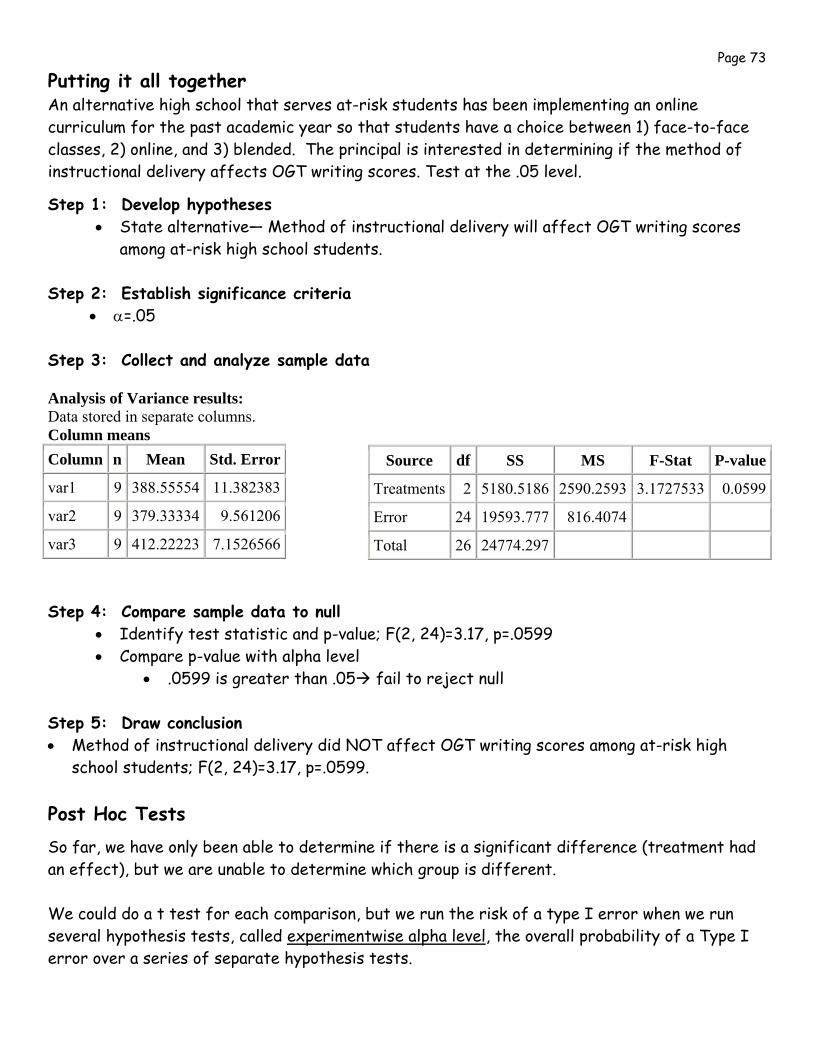
Page 73

Putting it all together An alternative high school that serves at-risk students has been implementing an online curriculum for the past academic year so that students have a choice between 1) face-to-face classes, 2) online, and 3) blended. The principal is interested in determining if the method of instructional delivery affects OGT writing scores. Test at the .05 level.

Step 1: Develop hypotheses • State alternative— Method of instructional delivery will affect OGT writing scores

among at-risk high school students. Step 2: Establish significance criteria

• α=.05

Step 3: Collect and analyze sample data Analysis of Variance results: Data stored in separate columns. Column means

Step 4: Compare sample data to null • Identify test statistic and p-value; F(2, 24)=3.17, p=.0599 • Compare p-value with alpha level

• .0599 is greater than .05 fail to reject null

Step 5: Draw conclusion • Method of instructional delivery did NOT affect OGT writing scores among at-risk high

school students; F(2, 24)=3.17, p=.0599. Post Hoc Tests

So far, we have only been able to determine if there is a significant difference (treatment had an effect), but we are unable to determine which group is different. We could do a t test for each comparison, but we run the risk of a type I error when we run several hypothesis tests, called experimentwise alpha level, the overall probability of a Type I error over a series of separate hypothesis tests.

Column n Mean Std. Error

var1 9 388.55554 11.382383

var2 9 379.33334 9.561206

var3 9 412.22223 7.1526566

Source df SS MS F-Stat P-value

Treatments 2 5180.5186 2590.2593 3.1727533 0.0599

Error 24 19593.777 816.4074

Total 26 24774.297

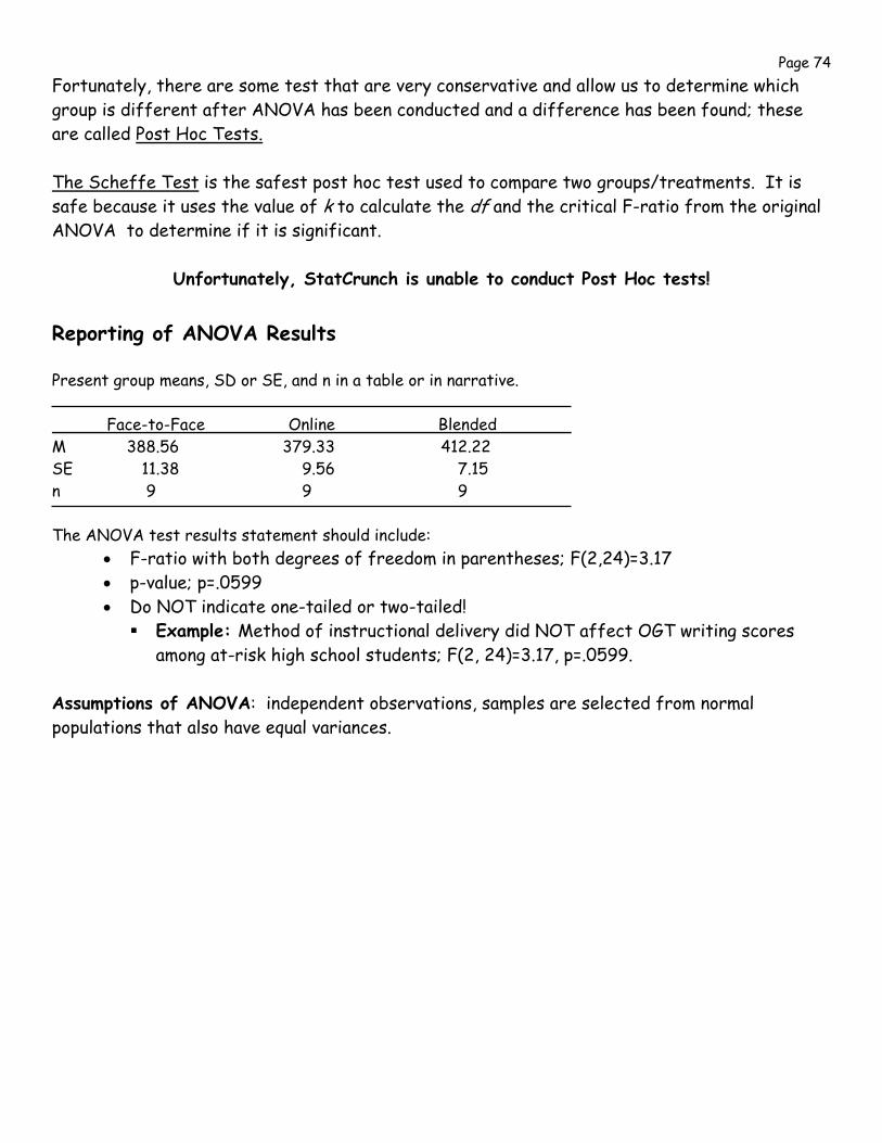
Page 74 Fortunately, there are some test that are very conservative and allow us to determine which group is different after ANOVA has been conducted and a difference has been found; these are called Post Hoc Tests. The Scheffe Test is the safest post hoc test used to compare two groups/treatments. It is safe because it uses the value of k to calculate the df and the critical F-ratio from the original ANOVA to determine if it is significant.

Unfortunately, StatCrunch is unable to conduct Post Hoc tests! Reporting of ANOVA Results Present group means, SD or SE, and n in a table or in narrative. Face-to-Face Online Blended M 388.56 379.33 412.22 SE 11.38 9.56 7.15 n 9 9 9 The ANOVA test results statement should include:

• F-ratio with both degrees of freedom in parentheses; F(2,24)=3.17 • p-value; p=.0599 • Do NOT indicate one-tailed or two-tailed!

Example: Method of instructional delivery did NOT affect OGT writing scores among at-risk high school students; F(2, 24)=3.17, p=.0599.

Assumptions of ANOVA: independent observations, samples are selected from normal populations that also have equal variances.

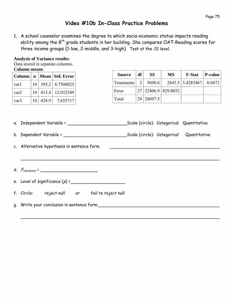
Page 75

Video #10b In-Class Practice Problems 1. A school counselor examines the degree to which socio-economic status impacts reading

ability among the 8th grade students in her building. She compares OAT-Reading scores for three income groups (1-low, 2-middle, and 3-high). Test at the .01 level.

Analysis of Variance results: Data stored in separate columns. Column means

a. Independent Variable = Scale (circle): Categorical Quantitative b. Dependent Variable = Scale (circle): Categorical Quantitative c. Alternative hypothesis in sentence form. d. Fcalculated = e. Level of significance (p) = f. Circle: reject null or fail to reject null g. Write your conclusion in sentence form.


var1 10 395.2 6.7508025

var2 10 413.4 12.032549

var3 10 428.9 7.655717


Treatments 2 5690.6 2845.3 3.4285467 0.0471

Error 27 22406.9 829.8852

Total 29 28097.5

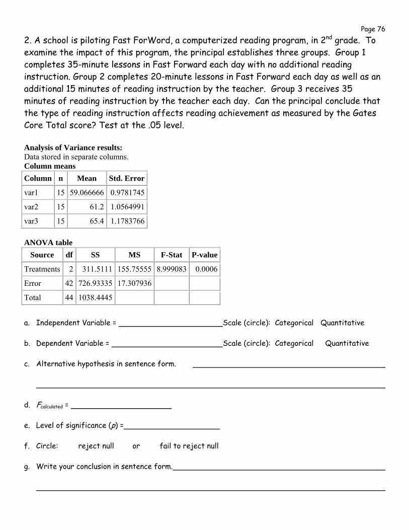
Page 76 2. A school is piloting Fast ForWord, a computerized reading program, in 2nd grade. To examine the impact of this program, the principal establishes three groups. Group 1 completes 35-minute lessons in Fast Forward each day with no additional reading instruction. Group 2 completes 20-minute lessons in Fast Forward each day as well as an additional 15 minutes of reading instruction by the teacher. Group 3 receives 35 minutes of reading instruction by the teacher each day. Can the principal conclude that the type of reading instruction affects reading achievement as measured by the Gates Core Total score? Test at the .05 level. Analysis of Variance results: Data stored in separate columns. Column means

ANOVA table

a. Independent Variable = Scale (circle): Categorical Quantitative b. Dependent Variable = Scale (circle): Categorical Quantitative c. Alternative hypothesis in sentence form. d. Fcalculated = e. Level of significance (p) = f. Circle: reject null or fail to reject null g. Write your conclusion in sentence form.


var1 15 59.066666 0.9781745

var2 15 61.2 1.0564991

var3 15 65.4 1.1783766


Treatments 2 311.5111 155.75555 8.999083 0.0006

Error 42 726.93335 17.307936

Total 44 1038.4445

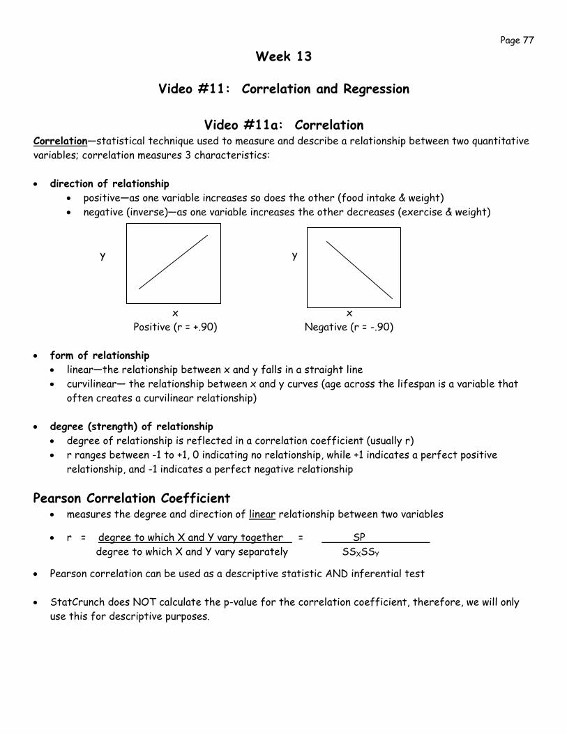
Page 77

Week 13

Video #11: Correlation and Regression

Video #11a: Correlation Correlation—statistical technique used to measure and describe a relationship between two quantitative variables; correlation measures 3 characteristics: • direction of relationship

• positive—as one variable increases so does the other (food intake & weight) • negative (inverse)—as one variable increases the other decreases (exercise & weight)

y y

x x Positive (r = +.90) Negative (r = -.90)

• form of relationship • linear—the relationship between x and y falls in a straight line • curvilinear— the relationship between x and y curves (age across the lifespan is a variable that

often creates a curvilinear relationship)

• degree (strength) of relationship • degree of relationship is reflected in a correlation coefficient (usually r) • r ranges between -1 to +1, 0 indicating no relationship, while +1 indicates a perfect positive

relationship, and -1 indicates a perfect negative relationship Pearson Correlation Coefficient

• measures the degree and direction of linear relationship between two variables

• r = degree to which X and Y vary together = SP degree to which X and Y vary separately SSXSSY

• Pearson correlation can be used as a descriptive statistic AND inferential test • StatCrunch does NOT calculate the p-value for the correlation coefficient, therefore, we will only

use this for descriptive purposes.

Page 78

Interpreting Correlation Coefficient • does NOT measure cause and effect • when data have a limited range of scores, the value of the correlation can be exaggerated • interpreting strength of coefficient (practical significance):

• r > .8 is very strong • r = .6 - .79 is strong • r = .4 - .59 is fair • r < .39 is weak

Coefficient of Determination • r2 Describes how accurately one variable predicts the other, square r. • For example, if r=.60, then r2 = .36, which can be interpreted as 36% of the variability in Y

scores can be predicted from the relationship with X. • Measures the proportion of variability in one variable that can be determined from the

relationship with the other variable.

Video #11b: Regression

Regression Regression—statistical technique for finding the best-fitting straight line for a set of data; used when wanting to determine the ability of one variable to predict another variable (e.g., using SAT score to predict freshman college GPA) Regression line—line that represents the linear relationship; represented by a linear equation

• Y = a + bX, where a = Y-intercept and b=slope • Equation is used to calculate predicted values

Hypothesis Testing for Regression

• Null hypothesis states that the IV does not significantly predict the DV • Alternative hypothesis states that the IV does not significantly predict the DV

ANOVA test • Measures the significance of the model (IV) to predict the DV. • Interpret the F-ratio and p-value to determine significance.

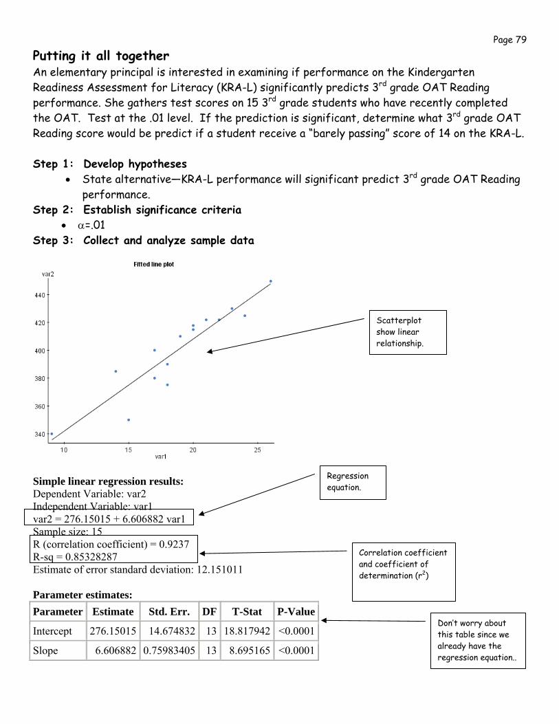
Page 79

Putting it all together An elementary principal is interested in examining if performance on the Kindergarten Readiness Assessment for Literacy (KRA-L) significantly predicts 3rd grade OAT Reading performance. She gathers test scores on 15 3rd grade students who have recently completed the OAT. Test at the .01 level. If the prediction is significant, determine what 3rd grade OAT Reading score would be predict if a student receive a “barely passing” score of 14 on the KRA-L. Step 1: Develop hypotheses

• State alternative—KRA-L performance will significant predict 3rd grade OAT Reading performance.

Step 2: Establish significance criteria • α=.01

Step 3: Collect and analyze sample data

Simple linear regression results: Dependent Variable: var2 Independent Variable: var1 var2 = 276.15015 + 6.606882 var1 Sample size: 15 R (correlation coefficient) = 0.9237 R-sq = 0.85328287 Estimate of error standard deviation: 12.151011 Parameter estimates:

Parameter Estimate Std. Err. DF T-Stat P-Value

Intercept 276.15015 14.674832 13 18.817942 <0.0001

Slope 6.606882 0.75983405 13 8.695165 <0.0001

Scatterplot show linear relationship.

Regression equation.

Correlation coefficient and coefficient of determination (r2)

Don’t worry about this table since we already have the regression equation..

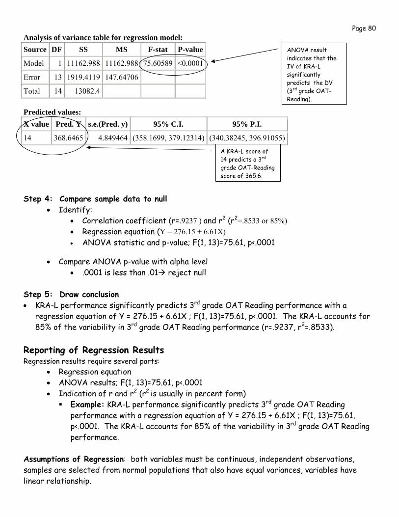
Page 80 Analysis of variance table for regression model:

Predicted values:

Step 4: Compare sample data to null

• Identify: • Correlation coefficient (r=.9237 ) and r2 (r2=.8533 or 85%) • Regression equation (Y = 276.15 + 6.61X) • ANOVA statistic and p-value; F(1, 13)=75.61, p<.0001

• Compare ANOVA p-value with alpha level

• .0001 is less than .01 reject null

Step 5: Draw conclusion • KRA-L performance significantly predicts 3rd grade OAT Reading performance with a

regression equation of Y = 276.15 + 6.61X ; F(1, 13)=75.61, p<.0001. The KRA-L accounts for 85% of the variability in 3rd grade OAT Reading performance (r=.9237, r2=.8533).

Reporting of Regression Results Regression results require several parts:

• Regression equation • ANOVA results; F(1, 13)=75.61, p<.0001 • Indication of r and r2 (r2 is usually in percent form)

Example: KRA-L performance significantly predicts 3rd grade OAT Reading performance with a regression equation of Y = 276.15 + 6.61X ; F(1, 13)=75.61, p<.0001. The KRA-L accounts for 85% of the variability in 3rd grade OAT Reading performance.

Assumptions of Regression: both variables must be continuous, independent observations, samples are selected from normal populations that also have equal variances, variables have linear relationship.

Source DF SS MS F-stat P-value

Model 1 11162.988 11162.988 75.60589 <0.0001

Error 13 1919.4119 147.64706

Total 14 13082.4

X value Pred. Y s.e.(Pred. y) 95% C.I. 95% P.I.

14 368.6465 4.849464 (358.1699, 379.12314) (340.38245, 396.91055)

ANOVA result indicates that the IV of KRA-L significantly predicts the DV (3rd grade OAT-Reading).

A KRA-L score of 14 predicts a 3rd grade OAT-Reading score of 365.6.

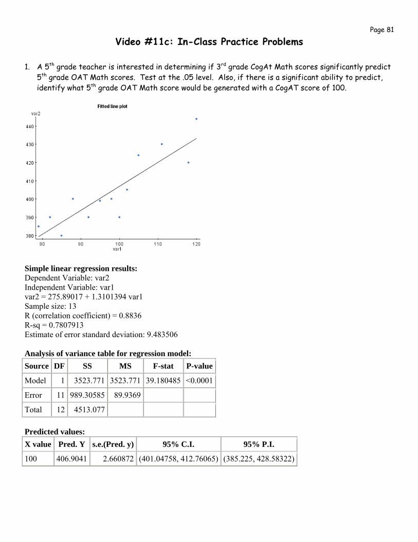
Page 81

Video #11c: In-Class Practice Problems

1. A 5th grade teacher is interested in determining if 3rd grade CogAt Math scores significantly predict 5th grade OAT Math scores. Test at the .05 level. Also, if there is a significant ability to predict, identify what 5th grade OAT Math score would be generated with a CogAT score of 100.

Simple linear regression results: Dependent Variable: var2 Independent Variable: var1 var2 = 275.89017 + 1.3101394 var1 Sample size: 13 R (correlation coefficient) = 0.8836 R-sq = 0.7807913 Estimate of error standard deviation: 9.483506 Analysis of variance table for regression model:

Predicted values:


Model 1 3523.771 3523.771 39.180485 <0.0001

Error 11 989.30585 89.9369

Total 12 4513.077


100 406.9041 2.660872 (401.04758, 412.76065) (385.225, 428.58322)

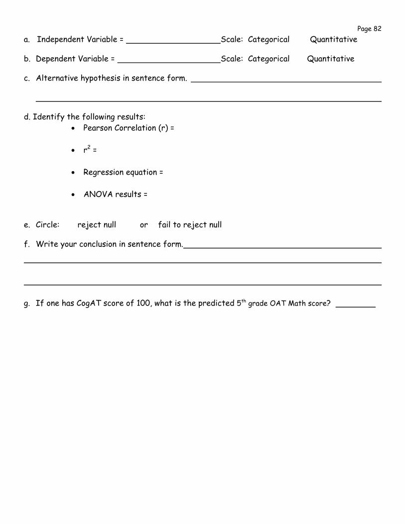
Page 82 a. Independent Variable = Scale: Categorical Quantitative b. Dependent Variable = Scale: Categorical Quantitative c. Alternative hypothesis in sentence form. d. Identify the following results:

• Pearson Correlation (r) =

• r2 =

• Regression equation =

• ANOVA results =

e. Circle: reject null or fail to reject null f. Write your conclusion in sentence form.

g. If one has CogAT score of 100, what is the predicted 5th grade OAT Math score?

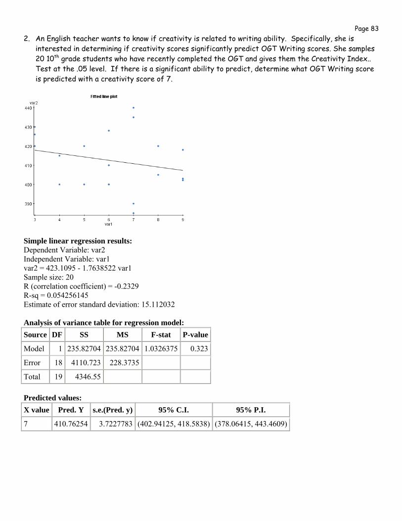
Page 83 2. An English teacher wants to know if creativity is related to writing ability. Specifically, she is

interested in determining if creativity scores significantly predict OGT Writing scores. She samples 20 10th grade students who have recently completed the OGT and gives them the Creativity Index.. Test at the .05 level. If there is a significant ability to predict, determine what OGT Writing score is predicted with a creativity score of 7.

Simple linear regression results: Dependent Variable: var2 Independent Variable: var1 var2 = 423.1095 - 1.7638522 var1 Sample size: 20 R (correlation coefficient) = -0.2329 R-sq = 0.054256145 Estimate of error standard deviation: 15.112032 Analysis of variance table for regression model:

Predicted values:


Model 1 235.82704 235.82704 1.0326375 0.323

Error 18 4110.723 228.3735

Total 19 4346.55


7 410.76254 3.7227783 (402.94125, 418.5838) (378.06415, 443.4609)

Page 84 a. Independent Variable = Scale: Categorical Quantitative b. Dependent Variable = Scale: Categorical Quantitative c. Alternative hypothesis in sentence form. d. Identify the following results:

• Pearson Correlation (r) =

• r2 =

• Regression equation =

• ANOVA results =

e. Circle: reject null or fail to reject null f. Write your conclusion in sentence form.

g. If one has creativity score of 7, what is the predicted OGT writing score?

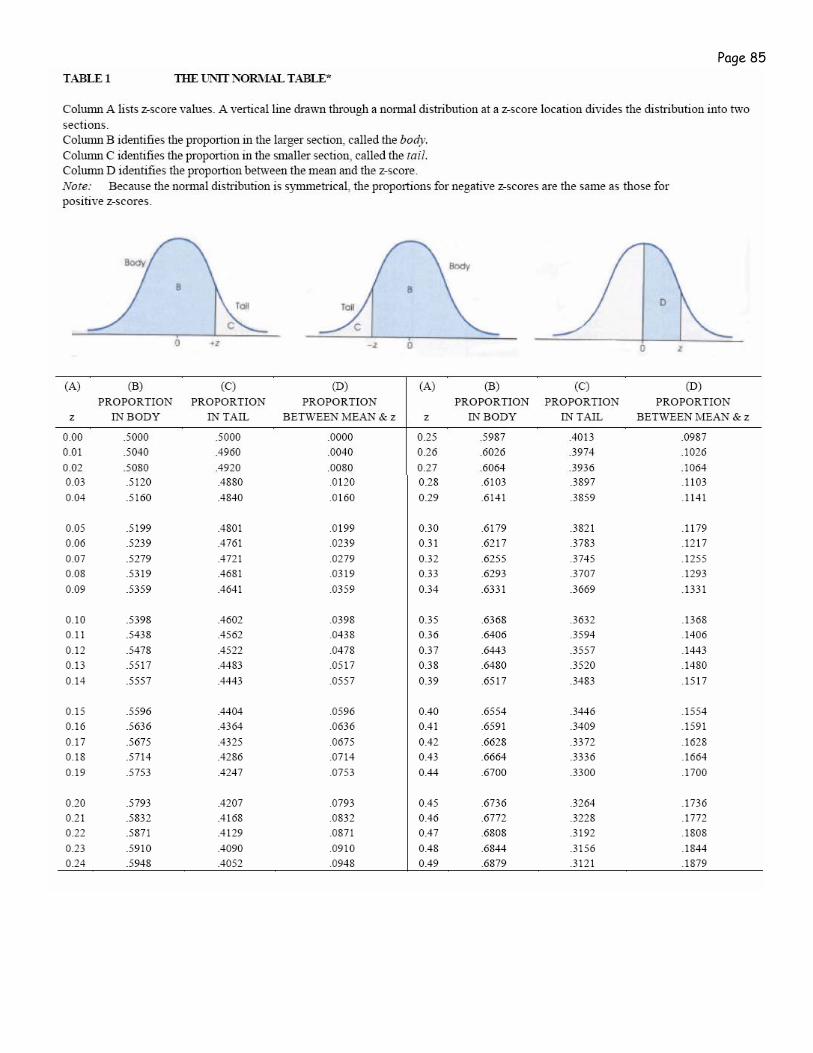
Page 85

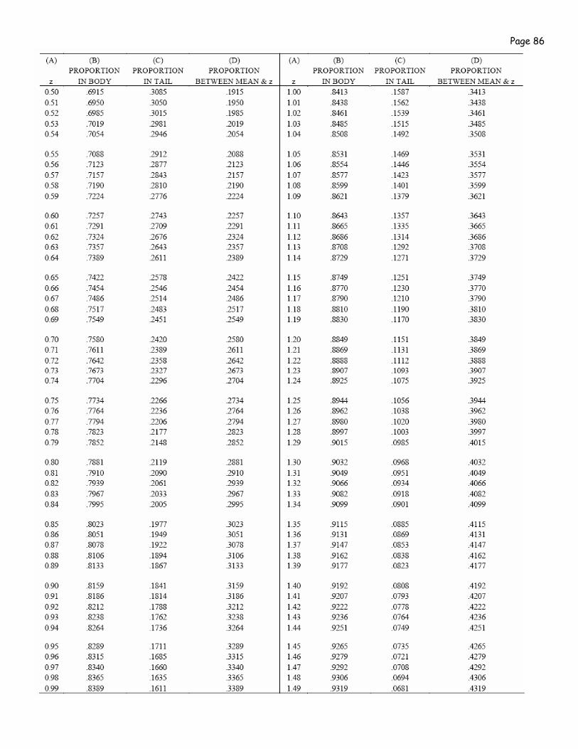
Page 86

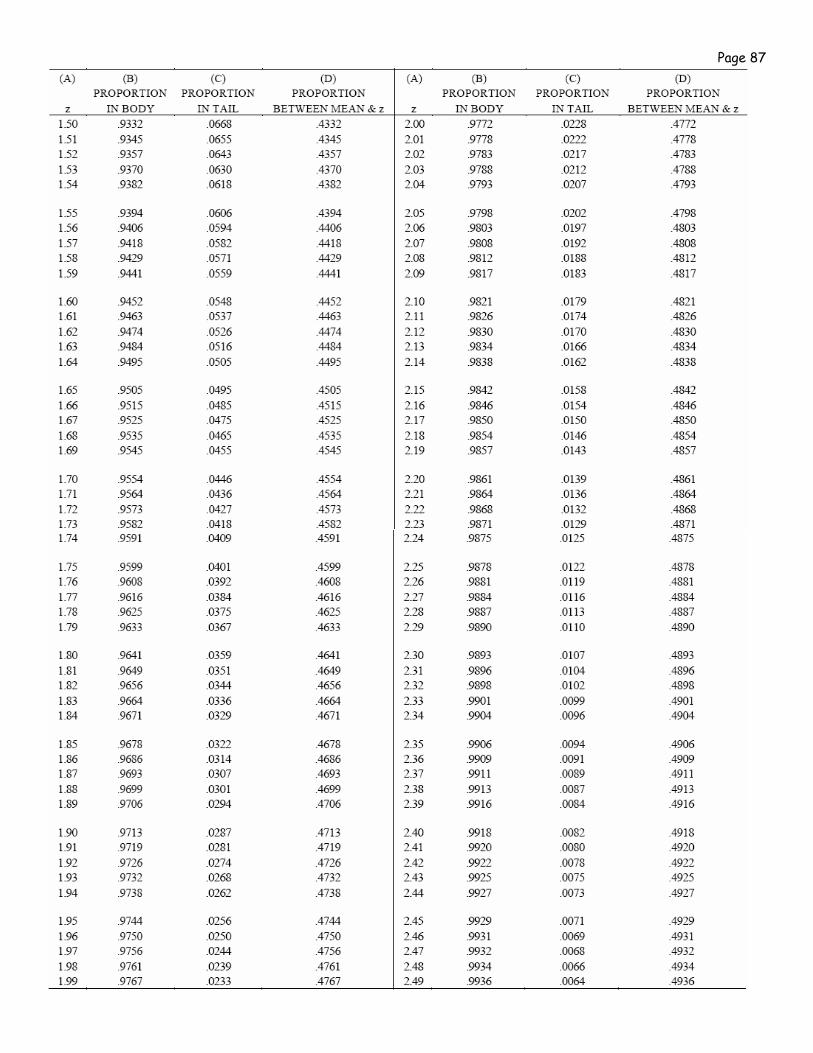
Page 87

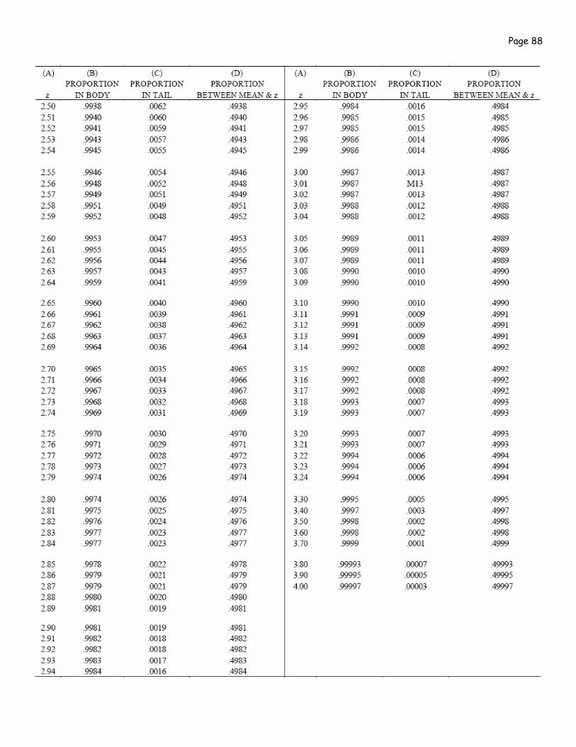
Page 88

Documents

EDFI 6450 Using Assessment & Research to Improve Practice