Embed Size (px)
DESCRIPTION
Stereo camera calibration for industrial robot
Citation preview
ROBOT
CALIBRATION Determination of Robot Motion Accuracy Using Artificial
Perception Devices
ECSE 475-DESIGN PROJECT II – Final Report Intakhab Alam - 260271961
Radu Sturzu - 260330228
Tabassum Mizan – 260345222
(under the supervision of Professor Frank P. Ferrie)
ECSE
475
16/4/2013
Design Project 2-Final Report
2
Abstract
The Gantry automated robot is an industrial robot permitting motions with six degrees of freedom which
can find applications in many fields. As some tasks re very accuracy dependant, it is required to verify the
accuracy of the motions performed by the robot before making use of the robot on the field.
The purpose of this project is to determine the accuracy of the motions performed by a Gantry automated
robot across the X Y and Z axes. An off the shelf video capture device will be used to track LED lights
mounted on the robot’s arm as the robot moves through space. The motion patterns are written using
RAPLII as a programming language. A simple MATLAB interface that can operate the robot will be also
validated, improved and rendered more user-friendly to the common user.
Through familiarisation with the robot, its physical functioning and the programming behind it, as well
through research on various artificial imaging techniques and devices, protocols have been developed for
measuring the accuracy for single motions across the X, Y or Z axes al low movement speeds and for
validating the MATLAB interface. During the second part of the project, these protocols will be fine-
tuned, the MATLAB interface will be improved and protocols will be developed for determining the
accuracy of the robot for compound motions at various speeds.

Design Project 2-Final Report
3
Acknowledgements
We would like to acknowledge Professor Frank. P. Ferrie and the Department of Electrical and Computer
Engineering and the Centre for Intelligent Machines (CIM) for giving us the opportunity to work on this
project. We would also like to extend our appreciation to Professor Roni Khazaka for guiding us
throughout the project.
Design Project 2-Final Report
4
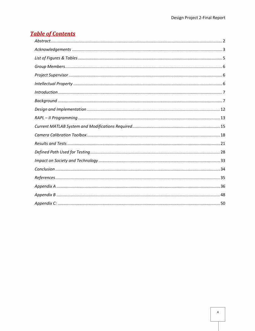
Table of Contents Abstract ............................................................................................................................................... 2
Acknowledgements ............................................................................................................................. 3
List of Figures & Tables ........................................................................................................................ 5
Group Members................................................................................................................................... 6
Project Supervisor ................................................................................................................................ 6
Intellectual Property ............................................................................................................................ 6
Introduction ......................................................................................................................................... 7
Background ......................................................................................................................................... 7
Design and Implementation ............................................................................................................... 12
RAPL – II Programming ...................................................................................................................... 13
Current MATLAB System and Modifications Required......................................................................... 15
Camera Calibration Toolbox ............................................................................................................... 18
Results and Tests ............................................................................................................................... 21
Defined Path Used for Testing ............................................................................................................ 28
Impact on Society and Technology ..................................................................................................... 33
Conclusion ......................................................................................................................................... 34
References ......................................................................................................................................... 35
Appendix A ........................................................................................................................................ 36
Appendix B ........................................................................................................................................ 48
Appendix C: ....................................................................................................................................... 50
Design Project 2-Final Report
5
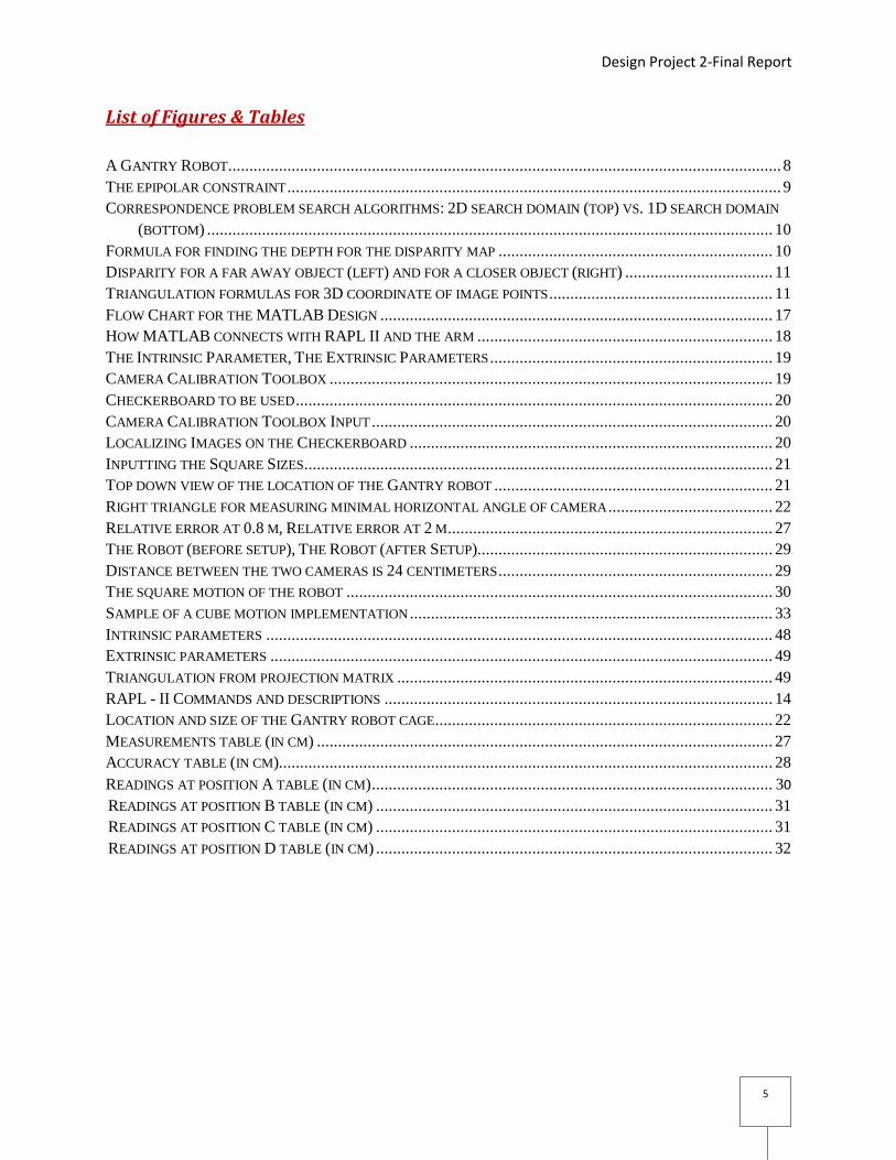
List of Figures & Tables
A GANTRY ROBOT ................................................................................................................................... 8
THE EPIPOLAR CONSTRAINT ..................................................................................................................... 9
CORRESPONDENCE PROBLEM SEARCH ALGORITHMS: 2D SEARCH DOMAIN (TOP) VS. 1D SEARCH DOMAIN
(BOTTOM) ...................................................................................................................................... 10
FORMULA FOR FINDING THE DEPTH FOR THE DISPARITY MAP ................................................................. 10
DISPARITY FOR A FAR AWAY OBJECT (LEFT) AND FOR A CLOSER OBJECT (RIGHT) ................................... 11
TRIANGULATION FORMULAS FOR 3D COORDINATE OF IMAGE POINTS ..................................................... 11
FLOW CHART FOR THE MATLAB DESIGN ............................................................................................. 17
HOW MATLAB CONNECTS WITH RAPL II AND THE ARM ...................................................................... 18
THE INTRINSIC PARAMETER, THE EXTRINSIC PARAMETERS ................................................................... 19
CAMERA CALIBRATION TOOLBOX ......................................................................................................... 19
CHECKERBOARD TO BE USED ................................................................................................................. 20
CAMERA CALIBRATION TOOLBOX INPUT ............................................................................................... 20
LOCALIZING IMAGES ON THE CHECKERBOARD ...................................................................................... 20
INPUTTING THE SQUARE SIZES ............................................................................................................... 21
TOP DOWN VIEW OF THE LOCATION OF THE GANTRY ROBOT .................................................................. 21
RIGHT TRIANGLE FOR MEASURING MINIMAL HORIZONTAL ANGLE OF CAMERA ....................................... 22
RELATIVE ERROR AT 0.8 M, RELATIVE ERROR AT 2 M ............................................................................. 27
THE ROBOT (BEFORE SETUP), THE ROBOT (AFTER SETUP)...................................................................... 29
DISTANCE BETWEEN THE TWO CAMERAS IS 24 CENTIMETERS ................................................................. 29
THE SQUARE MOTION OF THE ROBOT ..................................................................................................... 30
SAMPLE OF A CUBE MOTION IMPLEMENTATION ...................................................................................... 33
INTRINSIC PARAMETERS ........................................................................................................................ 48
EXTRINSIC PARAMETERS ....................................................................................................................... 49
TRIANGULATION FROM PROJECTION MATRIX ......................................................................................... 49
RAPL - II COMMANDS AND DESCRIPTIONS ............................................................................................ 14
LOCATION AND SIZE OF THE GANTRY ROBOT CAGE ................................................................................ 22
MEASUREMENTS TABLE (IN CM) ............................................................................................................ 27
ACCURACY TABLE (IN CM)..................................................................................................................... 28
READINGS AT POSITION A TABLE (IN CM) ............................................................................................... 30
READINGS AT POSITION B TABLE (IN CM) .............................................................................................. 31
READINGS AT POSITION C TABLE (IN CM) .............................................................................................. 31
READINGS AT POSITION D TABLE (IN CM) .............................................................................................. 32
Design Project 2-Final Report
6
Group Members
Name: Intakhab Alam Zeeshan
Student ID: 260271961
Course: Fall 2012 - ECSE-475-001 - Design Project II
Education: 4th year Bachelor of Electrical Engineering Student
Email: [email protected]
Name: Radu Sturzu
Student ID: 260330228
Course: Fall 2012 - ECSE-475-001 - Design Project II
Education: 4th year Bachelor of Electrical Engineering Student, Minor in Software Engineering
Email: [email protected]
Name: Tabassum Mizan
Student ID: 260345222
Course: Fall 2012 - ECSE-475-001 - Design Project II
Education: 4th year Bachelor of Electrical Engineering
Student Email: [email protected]
Project Supervisor
Supervisor: Professor Frank. P. Ferrie
Office: McConnell Engineering Building, Room 441
Department: Electrical and Computer Engineering and the Centre for Intelligent Machines (CIM)
Email: [email protected]
Tel: (514)398-6042
Intellectual Property
The intellectual scope for the software and hardware material, as well as all the employed knowledge
base, and any code employed or developed within this project has been decided by Professor Frank. P.
Ferrie. No attempt to divulge any of the previously listed outside of the team, for commercial or non-
commercial purposes, is to be made without the personal consent of the professor. However, the
documentation files on MATLAB, OpenCV or Python are freely available to the public.
Design Project 2-Final Report
7
Introduction
The project consists of finding the amount of error that a state-of-the-art industrial robotic arm produces
during operation. It will be programmed to perform specific movements and gestures around a given
space. If the movements do not take place precisely as desired, the amount of error that arises will be
measured and recorded. Using the data and the error generated, an “error mapping” will be created. The
robotic arm is operated by a series of motors that provide six degrees of freedom, with the inputs and
outputs being connected to a controller. Here the error is defined as the distance in X, Y, Z between the
actual location of the arm and the location computed by the software. The initial commands, as well as the
movement of the arm, are controlled through MATLAB.
Built with industrial use in mind, this project would be useful for a number of applications requiring
automated robotic arms, ranging from manipulation of hazardous substances to providing welding
tutorials to employees. As an outcome, it is expected that the error will be fully understood, allowing for
the necessary software and hardware calibrations to be performed, thus ensuring a flawless operation of
the equipment.
At this time, the project consists of two parts. The initial part translates to getting to gaining knowledge
about the environment and the commands that operate the robot, determining a preliminary protocol for
measuring the accuracy of the robot motions, which will be used by an existing Matlab interface. The
second part consists primarily of implementing the accuracy measurement protocol and testing it with a
series of robot movements, as implementing those changes inside the existing Matlab interface, as well
as rendering that interface as user friendly as possible. The required material comprises robotic arm itself,
with the necessary peripherals, measuring tools, documentation for both the Gantry robot and Matlab, as
well a lab featuring a computer containing MATLAB.
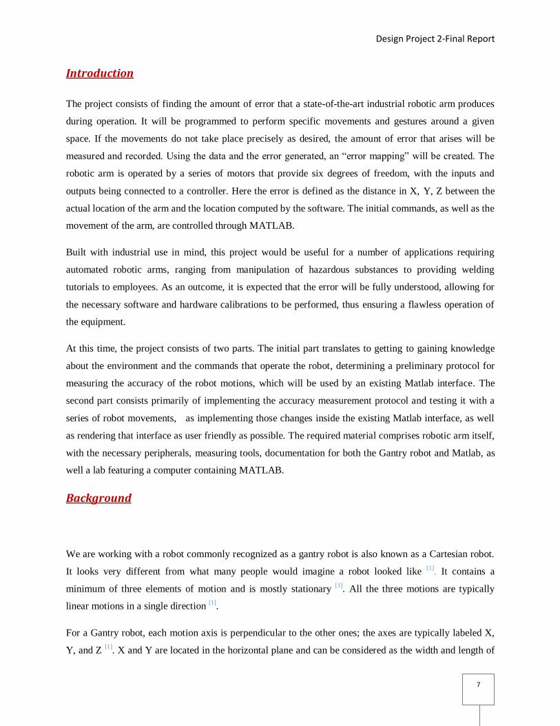
Background
We are working with a robot commonly recognized as a gantry robot is also known as a Cartesian robot.
It looks very different from what many people would imagine a robot looked like [1]
. It contains a
minimum of three elements of motion and is mostly stationary [1]
. All the three motions are typically
linear motions in a single direction [1]
.
For a Gantry robot, each motion axis is perpendicular to the other ones; the axes are typically labeled X,
Y, and Z [1]
. X and Y are located in the horizontal plane and can be considered as the width and length of
Design Project 2-Final Report
8
a box and Z is vertical, similar to the height of the box [1]
. The interior of this box is the working envelope
of the gantry robot and can perform various kinematics and operations on an item within the envelope [1]
.
First of all, measuring the accuracy of motion of the gantry robot requires a system for measuring the
position of the robot. Secondly, it also requires instructions that can move the gantry robot, as well as a
user interface that will control the gantry robot. The Gantry installation and operation manual offers the
basic necessary knowledge in understanding how the robot works, how it interfaces with the user as well
as the outside world. It also offers information on safety measures, as well as how to use the teaching
pendant, which is a remote control, designed to interface with the robot through a serial port.
All the programming instructions to be used with the robot are fully documented in the RAPLII
Programming Manual. Most of the reading time by the team members was spent studying this section.
The Process Control Programming KIT deals with advanced functions for the Gantry controller, which is
not a requirement at the moment. Time will also be spent in future attempting to implement more
complicated commands, such as controlling the robot to perform more advanced motions, involving more
complex paths, as well as motions involving the Yaw, Pitch and Roll axes.
Figure 1: A Gantry Robot
Design Project 2-Final Report
9
A stereo camera system offers the possibility of measuring the position of a moving object in three
dimensions. It requires solving the correspondence problem, namely correctly determining which part of
the image recorded by one camera corresponds to which part of the image recorded by the other camera
[7].
Every stereo camera system requires these four steps before successfully mapping a two dimensional
camera image onto three dimensions [7]
, namely calibration, rectification, stereo correspondence and lastly
triangulation.
Calibration is the process of finding the intrinsic and the extrinsic parameters of the camera. Intrinsic
parameters include the focal length, image center, and the parameters of the lens distortion. The extrinsic
parameters consist of finding the correct relative positions between the left and the right cameras.
Rectification involves using the results from the calibration step for removing lens distortion, as well as
using those results for aligning the two cameras: this latter step allows us to use the epipolar constraint in
order to solve the correspondence problem with a significantly lower computational cost.
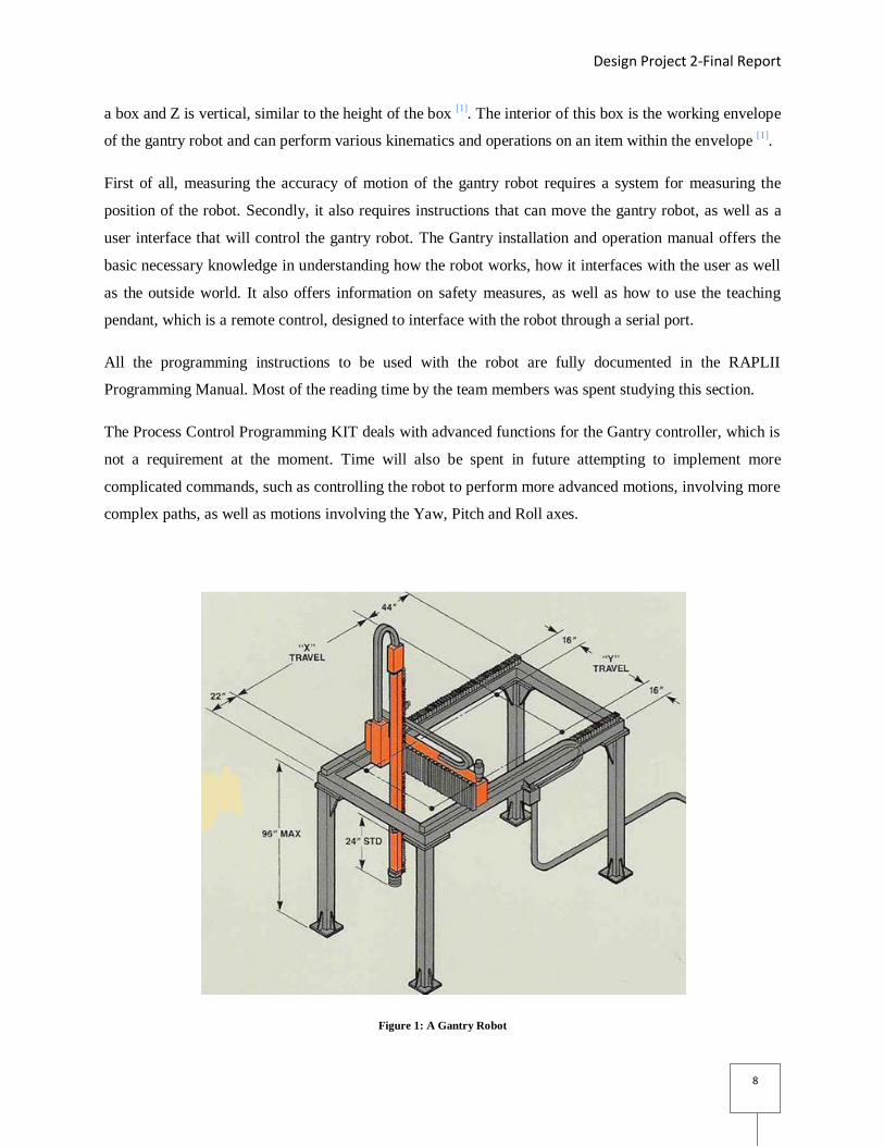
The epipolar constraint [7]
tells us that the correspondence for a point belonging to the red line of sight of
the image recorded by the left camera lies on the green light of sight of the image recorded by the right
camera, as seen in Figure 2.
Figure 2: The epipolar constraint
Design Project 2-Final Report
10
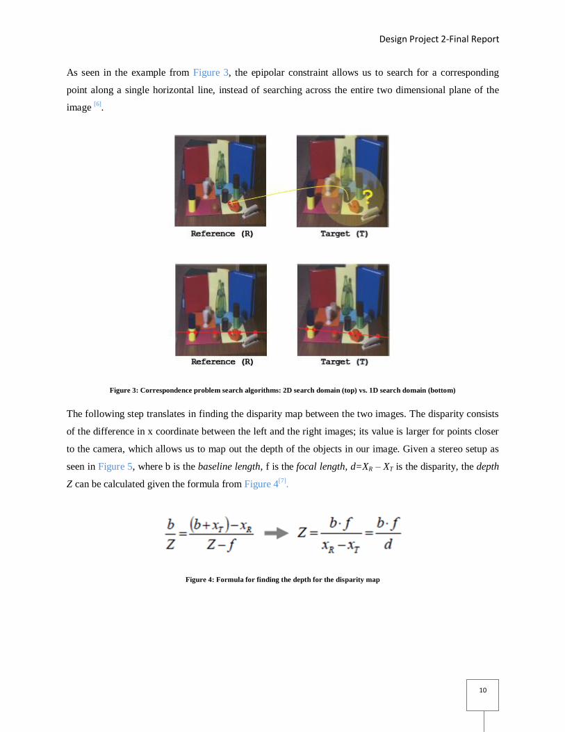
As seen in the example from Figure 3, the epipolar constraint allows us to search for a corresponding
point along a single horizontal line, instead of searching across the entire two dimensional plane of the
image [6]
.
Figure 3: Correspondence problem search algorithms: 2D search domain (top) vs. 1D search domain (bottom)
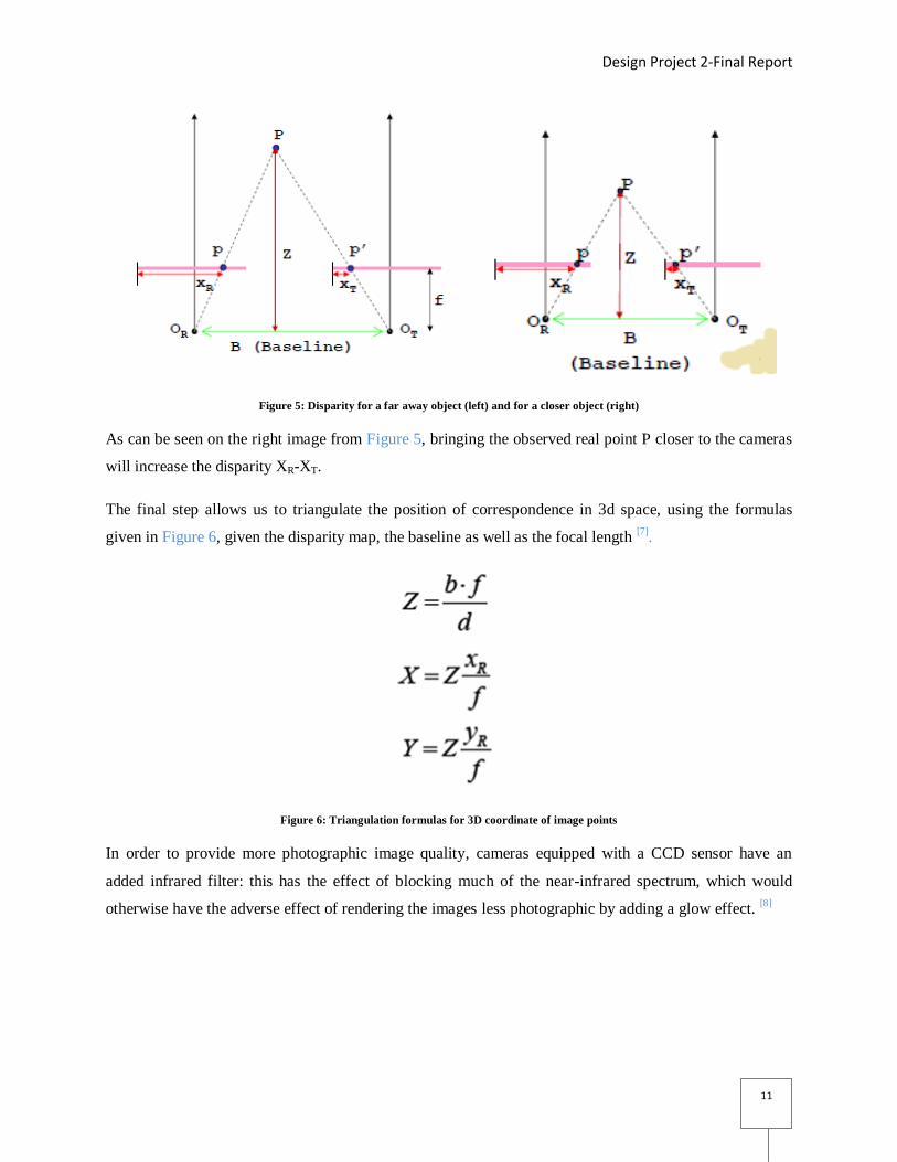
The following step translates in finding the disparity map between the two images. The disparity consists
of the difference in x coordinate between the left and the right images; its value is larger for points closer
to the camera, which allows us to map out the depth of the objects in our image. Given a stereo setup as
seen in Figure 5, where b is the baseline length, f is the focal length, d=XR – XT is the disparity, the depth
Z can be calculated given the formula from Figure 4[7]
.
Figure 4: Formula for finding the depth for the disparity map
Design Project 2-Final Report
11
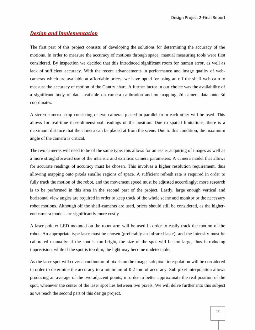
Figure 5: Disparity for a far away object (left) and for a closer object (right)
As can be seen on the right image from Figure 5, bringing the observed real point P closer to the cameras
will increase the disparity XR-XT.
The final step allows us to triangulate the position of correspondence in 3d space, using the formulas
given in Figure 6, given the disparity map, the baseline as well as the focal length [7]
.
Figure 6: Triangulation formulas for 3D coordinate of image points
In order to provide more photographic image quality, cameras equipped with a CCD sensor have an
added infrared filter: this has the effect of blocking much of the near-infrared spectrum, which would
otherwise have the adverse effect of rendering the images less photographic by adding a glow effect. [8]
Design Project 2-Final Report
12
Design and Implementation
The first part of this project consists of developing the solutions for determining the accuracy of the
motions. In order to measure the accuracy of motions through space, manual measuring tools were first
considered. By inspection we decided that this introduced significant room for human error, as well as
lack of sufficient accuracy. With the recent advancements in performance and image quality of web-
cameras which are available at affordable prices, we have opted for using an off the shelf web cam to
measure the accuracy of motion of the Gantry chart. A further factor in our choice was the availability of
a significant body of data available on camera calibration and on mapping 2d camera data onto 3d
coordinates.
A stereo camera setup consisting of two cameras placed in parallel from each other will be used. This
allows for real-time three-dimensional readings of the position. Due to spatial limitations, there is a
maximum distance that the camera can be placed at from the scene. Due to this condition, the maximum
angle of the camera is critical.
The two cameras will need to be of the same type; this allows for an easier acquiring of images as well as
a more straightforward use of the intrinsic and extrinsic camera parameters. A camera model that allows
for accurate readings of accuracy must be chosen. This involves a higher resolution requirement, thus
allowing mapping onto pixels smaller regions of space. A sufficient refresh rate is required in order to
fully track the motion of the robot, and the movement speed must be adjusted accordingly; more research
is to be performed in this area in the second part of the project. Lastly, large enough vertical and
horizontal view angles are required in order to keep track of the whole scene and monitor or the necessary
robot motions. Although off the shelf-cameras are used, prices should still be considered, as the higher-
end camera models are significantly more costly.
A laser pointer LED mounted on the robot arm will be used in order to easily track the motion of the
robot. An appropriate type laser must be chosen (preferably an infrared laser), and the intensity must be
calibrated manually: if the spot is too bright, the size of the spot will be too large, thus introducing
imprecision, while if the spot is too dim, the light may become undetectable.
As the laser spot will cover a continuum of pixels on the image, sub pixel interpolation will be considered
in order to determine the accuracy to a minimum of 0.2 mm of accuracy. Sub pixel interpolation allows
producing an average of the two adjacent points, in order to better approximate the real position of the
spot, whenever the center of the laser spot lies between two pixels. We will delve further into this subject
as we reach the second part of this design project.
Design Project 2-Final Report
13
In order to implement the stereo visions algorithm, the Camera Calibration Toolbox for Matlab, as well as
Open Source Camera Vision applications is being considered. [9]
A black and white check board will be
used for the calibration step.
RAPL – II Programming
RAPL – II, also known as Robotic Automation Programming Language, is a CRS proprietary language. It
is designed for robot systems application due to its ease of automation. The programming format is line
structured much like the BASIC structure. It is very user friendly due to English like commands.
RAPL II has many interesting features, such as, efficient coding structure for most effective use of
memory, alternate command identifiers and lastly advanced mathematical expressions. For experienced
programmer, this RAPL II programme is similar with basic programming, such as C.
Although it has numerous advantages, RAPL – II has a few key shortcomings. It only allows execution of
one main function and does not allow any subroutines. Case statements are also not available to use thus
greatly limiting efficient control flow. This greatly reduces the programming capability in RAPL – II.
RAPL – II provides parameters that define the robot coordinate system, i.e. x, y and z axes. It provides
commands using which the robot can be easily calibrated and localized. There are two modes of
operation:
a) Manual Mode: Using a teaching pendant (controller) provided with the robot, the robot can be
moved in the x, y and z directions by pressing buttons.
b) Line editor: Our project requires automatic control and movement of the robot. The line editor
allows us to easily send automatic commands and will be used primarily in the project.
RAPL – II provides multiple commands to control the robot. Although there are numerous commands
available to us, the most important ones are described in Table 1.
RAPL – II has defined different workspace environments:
a) Joint – Coordinate Systems: The A255 robot system uses this coordinate system. This series
consists of 5 different revolute joints. The zero positions for the respective joints are located at
the midpoints.
Design Project 2-Final Report
14
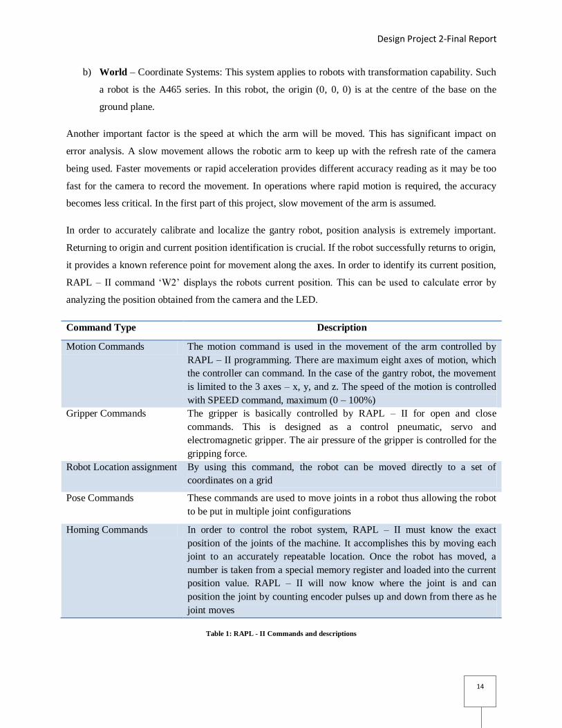
b) World – Coordinate Systems: This system applies to robots with transformation capability. Such
a robot is the A465 series. In this robot, the origin (0, 0, 0) is at the centre of the base on the
ground plane.
Another important factor is the speed at which the arm will be moved. This has significant impact on
error analysis. A slow movement allows the robotic arm to keep up with the refresh rate of the camera
being used. Faster movements or rapid acceleration provides different accuracy reading as it may be too
fast for the camera to record the movement. In operations where rapid motion is required, the accuracy
becomes less critical. In the first part of this project, slow movement of the arm is assumed.
In order to accurately calibrate and localize the gantry robot, position analysis is extremely important.
Returning to origin and current position identification is crucial. If the robot successfully returns to origin,
it provides a known reference point for movement along the axes. In order to identify its current position,
RAPL – II command ‘W2’ displays the robots current position. This can be used to calculate error by
analyzing the position obtained from the camera and the LED.
Command Type Description
Motion Commands The motion command is used in the movement of the arm controlled by
RAPL – II programming. There are maximum eight axes of motion, which
the controller can command. In the case of the gantry robot, the movement
is limited to the 3 axes – x, y, and z. The speed of the motion is controlled
with SPEED command, maximum (0 – 100%)
Gripper Commands The gripper is basically controlled by RAPL – II for open and close
commands. This is designed as a control pneumatic, servo and
electromagnetic gripper. The air pressure of the gripper is controlled for the
gripping force.
Robot Location assignment By using this command, the robot can be moved directly to a set of
coordinates on a grid
Pose Commands These commands are used to move joints in a robot thus allowing the robot
to be put in multiple joint configurations
Homing Commands In order to control the robot system, RAPL – II must know the exact
position of the joints of the machine. It accomplishes this by moving each
joint to an accurately repeatable location. Once the robot has moved, a
number is taken from a special memory register and loaded into the current
position value. RAPL – II will now know where the joint is and can
position the joint by counting encoder pulses up and down from there as he
joint moves
Table 1: RAPL - II Commands and descriptions
Design Project 2-Final Report
15
Current MATLAB System and Modifications Required
MATLAB is relatively easy to learn and is optimized to be relatively quick when performing matrix
operations and in some cases may behave like a calculator or as a programming language. It is an
interpreted language so errors are easier to fix. Hence, all the measurements from the external sensors will
be feed in into the MATLAB script to produce results. It does have a few limitations hence it will be
combined with RAPL II program and command lines to make the process more efficient and user-
friendly.
The MATLAB session currently present in the lab is capable to calibrate the gantry robot. It can take an
(Nx6) matrix as an input and can send the command through RAPL II programming, which activates the
kinematics of the robot as per the commands. It also allows us to change the speed parameters as well as
based on the position of the robot, can provide us a 3-dimensional picture of its location.
Operating the machine introduced us to the different limitations and abnormal behaviors the robot arm is
subjected to. The abnormal behavior comes from the fact that testing was not done to the fullest due to
availability of resources. Initially, all work was done using the terminal interface of the robot. Later on it
was moved to the MATLAB interface since it provided us more information in real time and also aids on
obtaining the position of the robot in the virtual XYZ axis. This led us to a bug that was present in the
program that was already loaded and was used to connect the robot arm with the computer itself. The
MATLAB program currently designed is a high level program and an extensive training is required
before a user can work hands-on with the automated arm. A simplified and more user-friendly MATLAB
session needs to be designed using the current one as the backbone to make sure when this industrial
robot is out in the field its basic functions can easily be mastered within a few hours so that work can
resume without any disruptions.
In midst of all the actions it can currently perform, the current system does not allow us to verify if the
robot has indeed made to its final position as per its commands or not. It does not provide us any
assurance of the accuracy and how off it was in terms of errors when reaching its designated position.
And since, everything is based on soft code it is not robust at all.
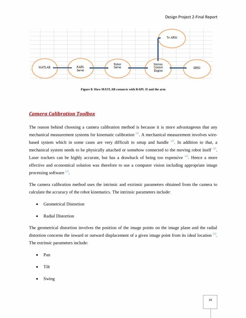
Figure 8 shows how MATLAB and RAPL II relate to each other.
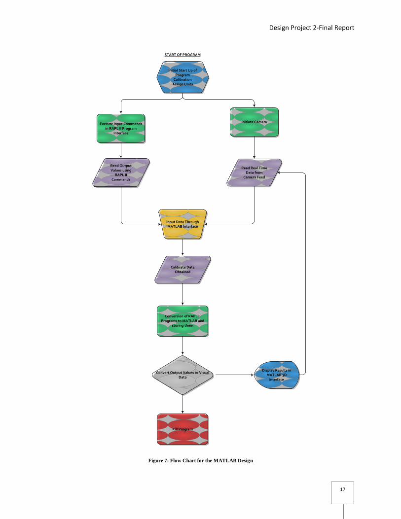
The flow chart in Figure 7 is the first foot print of what we will be aiming to design for the MATLAB
simulation. This starting point will be used as the reference point for all calculations hereafter.
Design Project 2-Final Report
16
In order to improve the performance of the current MATLAB program, the following design was
proposed as shown in Figure 4. It adds a camera calibration method on the current program. Initially
when the robot will be started, the arm will be homed and calibrated to a starting point. It localizes the
robot to an origin (0, 0, 0) from any position it previously resided on within the working envelope. Once
calibrated it assigns metric units to the robot, so that it runs on the same units as the program intends it to.
Once all this has been performed the system than connects itself to the MATLAB program, disabling the
manual controller.
Our program once executed will activate two processes at the same time. It will initiate the link with the
robot through the RAPL II program as well as initiate the camera being placed. The camera will be
feeding in data continuously, as the robot simultaneously moves through the working envelope. These
data will then be used to calculate the actual position of the robot in the envelope and also to find the
errors and accuracy associated with each movement.
The previous MATLAB program will be used as the backbone of the current design; hence it will retain
all other previous capabilities, such as displaying the results on a 3-dimensional grid.
Design Project 2-Final Report
17
Calibrate Data Obtained
Input Data Through MATLAB Interface
Initial Start Up of Program
CalibrationAssign Units
Conversion of RAPL II Programs to MATLAB and
storing them
Convert Output Values to Visual Data
Display Results in MATLAB 3D
interface
START OF PROGRAM
Read Real Time Data from
Camera Feed
Initiate Camera
Kill Program
Execute Input Commands in RAPL II Program
Interface
Read Output Values using
RAPL II Commands
Figure 7: Flow Chart for the MATLAB Design
Design Project 2-Final Report
18
Figure 8: How MATLAB connects with RAPL II and the arm
Camera Calibration Toolbox
The reason behind choosing a camera calibration method is because it is more advantageous that any
mechanical measurement systems for kinematic calibration [2]
. A mechanical measurement involves wire-
based system which in some cases are very difficult to setup and handle [2]
. In addition to that, a
mechanical system needs to be physically attached or somehow connected to the moving robot itself [2]
.
Laser trackers can be highly accurate, but has a drawback of being too expensive [2]
. Hence a more
effective and economical solution was therefore to use a computer vision including appropriate image
processing software [2]
.
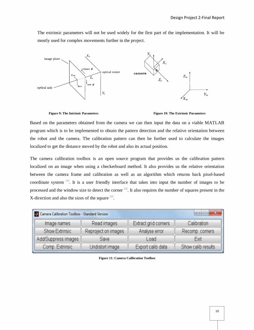
The camera calibration method uses the intrinsic and extrinsic parameters obtained from the camera to
calculate the accuracy of the robot kinematics. The intrinsic parameters include:
Geometrical Distortion
Radial Distortion
The geometrical distortion involves the position of the image points on the image plane and the radial
distortion concerns the inward or outward displacement of a given image point from its ideal location [3]
.
The extrinsic parameters include:
Pan
Tilt
Swing
Design Project 2-Final Report
19
The extrinsic parameters will not be used widely for the first part of the implementation. It will be
mostly used for complex movements further in the project.
Figure 9: The Intrinsic Parameters Figure 10: The Extrinsic Parameters
Based on the parameters obtained from the camera we can then input the data on a viable MATLAB
program which is to be implemented to obtain the pattern detection and the relative orientation between
the robot and the camera. The calibration pattern can then be further used to calculate the images
localized to get the distance moved by the robot and also its actual position.
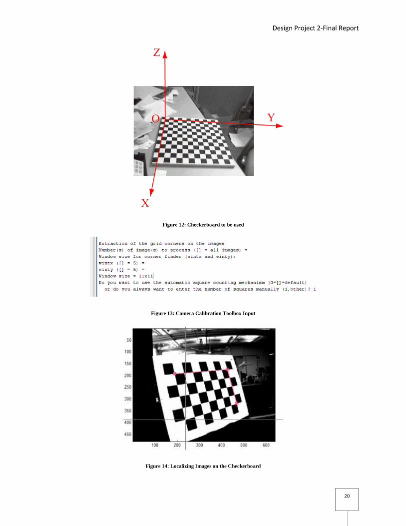
The camera calibration toolbox is an open source program that provides us the calibration pattern
localized on an image when using a checkerboard method. It also provides us the relative orientation
between the camera frame and calibration as well as an algorithm which returns back pixel-based
coordinate system [4]
. It is a user friendly interface that takes into input the number of images to be
processed and the window size to detect the corner [4]
. It also requires the number of squares present in the
X-direction and also the sizes of the square [4]
.
Figure 11: Camera Calibration Toolbox
Design Project 2-Final Report
20
Figure 12: Checkerboard to be used
Figure 13: Camera Calibration Toolbox Input
Figure 14: Localizing Images on the Checkerboard
Design Project 2-Final Report
21
Figure 15: Inputting the Square Sizes
Results and Tests
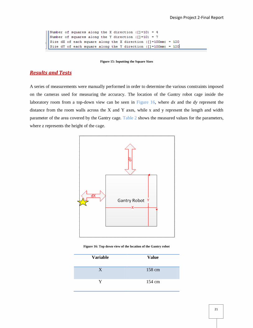
A series of measurements were manually performed in order to determine the various constraints imposed
on the cameras used for measuring the accuracy. The location of the Gantry robot cage inside the
laboratory room from a top-down view can be seen in Figure 16, where dx and the dy represent the
distance from the room walls across the X and Y axes, while x and y represent the length and width
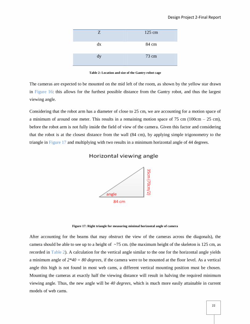
parameter of the area covered by the Gantry cage. Table 2 shows the measured values for the parameters,
where z represents the height of the cage.
Figure 16: Top down view of the location of the Gantry robot
Variable Value
X 158 cm
Y 154 cm
Design Project 2-Final Report
22
Z 125 cm
dx 84 cm
dy 73 cm
Table 2: Location and size of the Gantry robot cage
The cameras are expected to be mounted on the mid left of the room, as shown by the yellow star drawn
in Figure 16: this allows for the furthest possible distance from the Gantry robot, and thus the largest
viewing angle.
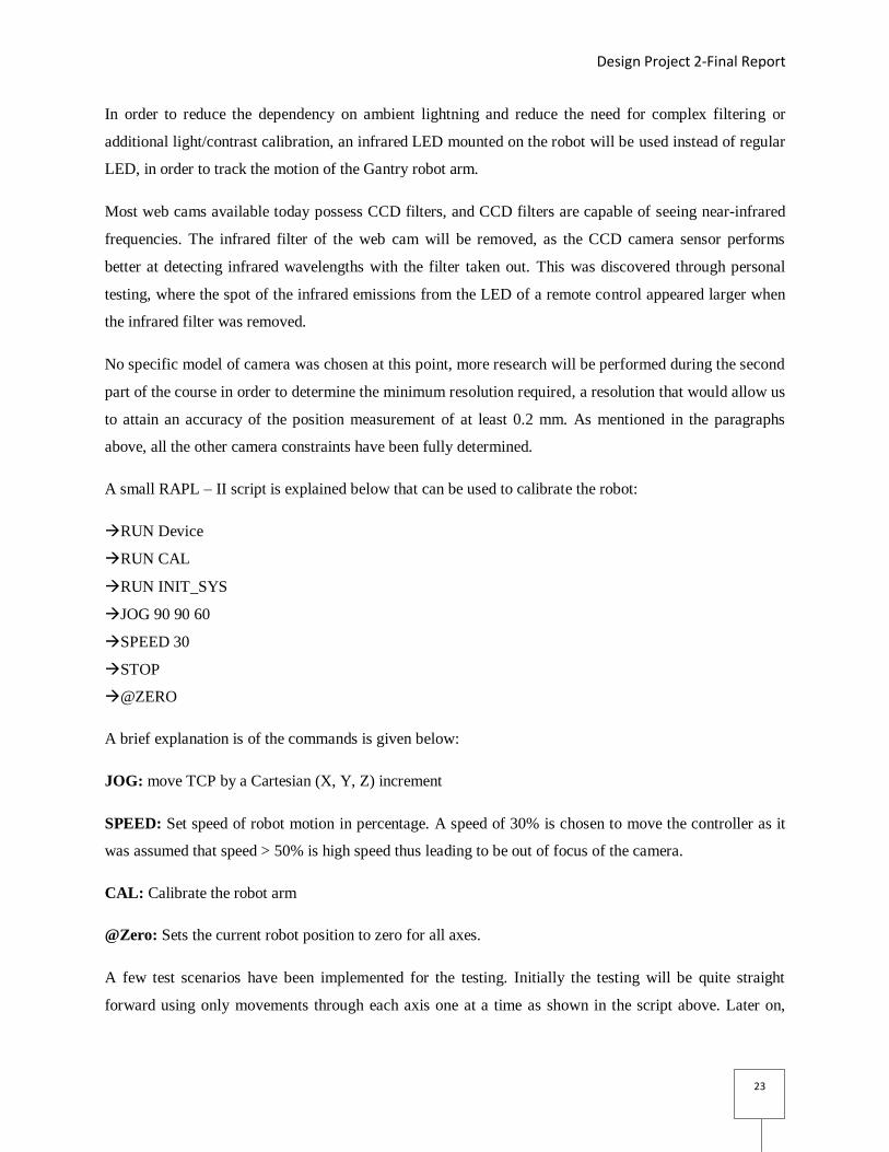
Considering that the robot arm has a diameter of close to 25 cm, we are accounting for a motion space of
a minimum of around one meter. This results in a remaining motion space of 75 cm (100cm – 25 cm),
before the robot arm is not fully inside the field of view of the camera. Given this factor and considering
that the robot is at the closest distance from the wall (84 cm), by applying simple trigonometry to the
triangle in Figure 17 and multiplying with two results in a minimum horizontal angle of 44 degrees.
Figure 17: Right triangle for measuring minimal horizontal angle of camera
After accounting for the beams that may obstruct the view of the cameras across the diagonals), the
camera should be able to see up to a height of ~75 cm. (the maximum height of the skeleton is 125 cm, as
recorded in Table 2). A calculation for the vertical angle similar to the one for the horizontal angle yields
a minimum angle of 2*40 = 80 degrees, if the camera were to be mounted at the floor level. As a vertical
angle this high is not found in most web cams, a different vertical mounting position must be chosen.
Mounting the cameras at exactly half the viewing distance will result in halving the required minimum
viewing angle. Thus, the new angle will be 40 degrees, which is much more easily attainable in current
models of web cams.
Design Project 2-Final Report
23
In order to reduce the dependency on ambient lightning and reduce the need for complex filtering or
additional light/contrast calibration, an infrared LED mounted on the robot will be used instead of regular
LED, in order to track the motion of the Gantry robot arm.
Most web cams available today possess CCD filters, and CCD filters are capable of seeing near-infrared
frequencies. The infrared filter of the web cam will be removed, as the CCD camera sensor performs
better at detecting infrared wavelengths with the filter taken out. This was discovered through personal
testing, where the spot of the infrared emissions from the LED of a remote control appeared larger when
the infrared filter was removed.
No specific model of camera was chosen at this point, more research will be performed during the second
part of the course in order to determine the minimum resolution required, a resolution that would allow us
to attain an accuracy of the position measurement of at least 0.2 mm. As mentioned in the paragraphs
above, all the other camera constraints have been fully determined.
A small RAPL – II script is explained below that can be used to calibrate the robot:
RUN Device
RUN CAL
RUN INIT_SYS
JOG 90 90 60
SPEED 30
STOP
@ZERO
A brief explanation is of the commands is given below:
JOG: move TCP by a Cartesian (X, Y, Z) increment
SPEED: Set speed of robot motion in percentage. A speed of 30% is chosen to move the controller as it
was assumed that speed > 50% is high speed thus leading to be out of focus of the camera.
CAL: Calibrate the robot arm
@Zero: Sets the current robot position to zero for all axes.
A few test scenarios have been implemented for the testing. Initially the testing will be quite straight
forward using only movements through each axis one at a time as shown in the script above. Later on,
Design Project 2-Final Report
24
more complex movements will be implemented after the robustness for our script has been identified.
Example of such a complex movement, could be a ``spline`` motion.
Even though the camera calibration toolbox algorithm does not give us exactly the errors and the accuracy
but it does give us the raw data and the TCP points of the localizations. Further implementation is
required to make sure that results are obtained in scaling metric units and also make sure users obtain the
best results in the simplest form.
This type of motion keeps the Tool Centre Point (TCP) moving in a straight line. As the geometry of the
tool or gripper which the robot carries can vary, RAPL – II provides programmers to define the tool tip
via TOOL coordinate programming.
As the second part of the project began, the old robot was unfortunately out of order, so the team is
waiting for new robot to be installed. During this period of time, we have received two C270 Logitech
cameras from our supervisor. We have experimented with acquiring images using the two cameras for
calibration and the Image Acquisition Toolbox from Matlab that make this possible. The cameras
function properly up to the maximum specified resolution of 1280x720. There was one problem where
attempting to use both USB cameras simultaneously due to both cameras attempting to access the same
USB controller. Upon changing the permissions of the ports accessed by the web-cams, the issue was
resolved with the help of Professor Ferrie. We have tried to use the GUI commands of the Matlab Image
Acquisition Toolbox for our image captures, but since it did not allow us to have two camera feeds active
at the same time, a script was instead; this script would acquire stereo images at pre-set time intervals
using manual triggering mode; this allows each of the cameras to perform the initialization process only
once at the beginning instead of before each image capture; as such, each subsequent image capture takes
less than 100 ms, versus around 1 second in automatic triggering mode. Using this, the image capturing
process is smoother and there is a significantly smaller delay between the capture of the left and right
images.
As we moved further in our design, we began investigating various camera calibration tools. We have
also installed the Camera Calibration Toolbox on Matlab, another option was OpenCV, which is C/C++
based. Initially we had found that the GUI of the Camera Calibration Toolbox had most of the features we
required, so at that point we did not need to use any code or any commands. We have experimented with
example images from camera calibration toolbox and we found the calibration process lengthy.
Design Project 2-Final Report
25
The new gantry robot was assembled at the start of the week. But it also had issues with the cables
connecting the arm to the main core. As a result, the whole robot malfunctioned. New cables were
ordered by Professor Ferrie in an attempt to fix one of the two gantry robots currently residing in the lab.
As no part of the gantry robot was at that point functional, Professor Ferrie has advised the team to look
into the other aspects of the project in more detail, such as the stereo calibration of the two cameras being
used. He has suggested and introduced us to one of his PhD students, Andrew Phan who has extensive
experience in the respective field. The team will be working and collaborating side-by-side with some his
work, in order to assemble an ideal stereo calibration system that will allow general gantry robots to
calibrate itself within its XYZ space at any light conditions.
So far the team has been using the Camera Calibration Toolbox as the pivotal software. But as per
Andrew Phan’s advice, the team will be using Open CV as well as Python to implement a more efficient
and better calibration system.
As time was short at this point in the semester, the team is implementing a new calculation method which
is different from what was planned initially. Specifically, a chessboard was used to track the position of
the Gantry robot hand, instead of using a laser pointer; since code already exists to detect the image points
of the chessboard corners, this simplifies the task of the team.
First, the cameras were mounted in parallel, at a certain distance (called baseline) from each other. A
series of images of the chessboard were acquired at various angles for a more accurate calibration. Our
script acquired the corners on these chessboard images as the image points, and generated a set of
corresponding 3d object points. Using these, the intrinsic parameters of each camera, such as the camera
matrix and the distortion coefficients were found. Afterwards, the stereo calibration was performed,
which calculated the translation and rotation vector that mapped the right camera image onto the left
camera image for the given baseline. Using rectification, the projection matrix was generated, which
allows for easy triangulation. Once this process was performed once for the given camera setup, the robot
hand.
A chessboard of the same size was then mounted on the robot; after each translational motion of the
robot, new projection points were acquired. With these points as well as the projection matrices initially
calculated, the world coordinates of the chessboard corners located on the robot hand are triangulated.
There was much trial and error, as there are two existing libraries for Python, some functions required
being available in only one of these two. Unfortunately, each uses different matrix representations; The
initial Python cv module employs matrices as type Mat, while the newer cv2 module uses matrices
Design Project 2-Final Report
26
belonging to a separate widely used module for numerical computations called NumPy (shorthand for
Numerical Python). As such, the team was required to carefully convert between the two matrix formats,
to carefully use either single or double precision floating point matrices as each function required, and to
reshape the size of some of the used matrices to fit the format of the required input/output of each
function. Furthermore, the documentation was spread out over multiple sources and thus inconsistent at
times, which slowed down our progress. Help was provided by Andrew Phan, as well as camera vision
enthusiasts found on various message boards. For a look at the formulas used by OpenCV, see Appendix
A. For examples from our code, see Appendix B.
Late in the project we decided to move our code onto the Ubuntu Linux platform. Unfortunately, after a
very lengthy installation process, as well as multiple issues of incompatibility issues with the camera
capture code from Python, we decided to revert back to our Windows based version of our code. Due to
this fact, we were not able to incorporate the results from our triangulation script inside the Gantry Robot
Matlab Interface found on the laboratory computer.
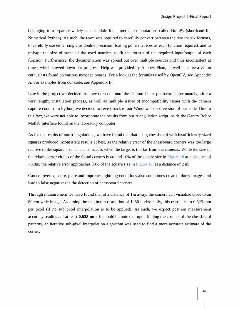
As for the results of our triangulations, we have found that that using chessboard with insufficiently sized
squares produced inconsistent results at best, as the relative error of the chessboard corners was too large
relative to the square size. This also occurs when the target is too far from the cameras. While the size of
the relative error circles of the found corners is around 10% of the square size in Figure 18 at a distance of
~0.8m, the relative error approaches 30% of the square size in Figure 19, at a distance of 2 m.
Camera overexposure, glare and improper lightning conditions also sometimes created blurry images and
lead to false negatives in the detection of chessboard corners.
Through measurement we have found that at a distance of 1m away, the camera can visualize close to an
80 cm wide image. Assuming the maximum resolution of 1280 horizontally, this translates to 0.625 mm
per pixel (if no sub pixel interpolation is to be applied). As such, we expect position measurement
accuracy readings of at least 0.625 mm. It should be note that upon finding the corners of the chessboard
patterns, an iterative sub-pixel interpolation algorithm was used to find a more accurate estimate of the
corner.
Design Project 2-Final Report
27
Figure 18: Relative error at 0.8 m Figure 19: Relative error at 2 m
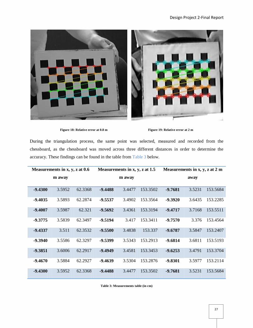
During the triangulation process, the same point was selected, measured and recorded from the
chessboard, as the chessboard was moved across three different distances in order to determine the
accuracy. These findings can be found in the table from Table 3 below.
Measurements in x, y, z at 0.6
m away
Measurements in x, y, z at 1.5
m away
Measurements in x, y, z at 2 m
away
-9.4300 3.5952 62.3368 -9.4488 3.4477 153.3502 -9.7681 3.5231 153.5684
-9.4035 3.5893 62.2874 -9.5537 3.4902 153.3564 -9.3920 3.6435 153.2285
-9.4007 3.5987 62.321 -9.5692 3.4361 153.3194 -9.4717 3.7168 153.5511
-9.3775 3.5839 62.3497 -9.5194 3.417 153.3411 -9.7570 3.376 153.4564
-9.4337 3.511 62.3532 -9.5500 3.4838 153.337 -9.6787 3.5847 153.2407
-9.3940 3.5586 62.3297 -9.5399 3.5343 153.2913 -9.6814 3.6811 153.5193
-9.3851 3.6006 62.2917 -9.4949 3.4581 153.3453 -9.6253 3.4791 153.3704
-9.4670 3.5884 62.2927 -9.4639 3.5304 153.2876 -9.8301 3.5977 153.2114
-9.4300 3.5952 62.3368 -9.4488 3.4477 153.3502 -9.7681 3.5231 153.5684
Table 3: Measurements table (in cm)
Design Project 2-Final Report
28
From these values, the error (in millimetres) from the average was calculated for the x, y and z axis at all
three distances. The results can be seen in the table from Table 4 upon inspection, it is to be noted that the
accuracy is around 0.25 mm at 0.6 m, increases to around 0.33 at 1.5 m away. Unfortunately, the error
increases to over 1 mm at 2 m away.
Error At 0.6 m away At 1.5 m away At 2 m
away
X axis 0.0241 0.0362 0.1157
Y axis 0.027559 0.0349 0.0968
Z axis 0.0192 0.0318 0.1305
Table 4: Accuracy table (in cm)
Defined Path Used for Testing
All the testing prior to this point was done with the robot being moved on one axis at a time. At this point,
when the calculation and triangulation was sufficiently robust, a defined path was implemented for the
robot, so to test our method on real life motions.
Initially, a square path was implemented, with the help of RAPL-II program. The points were predefined
so that the robot can recall them from the memory when the program is run.
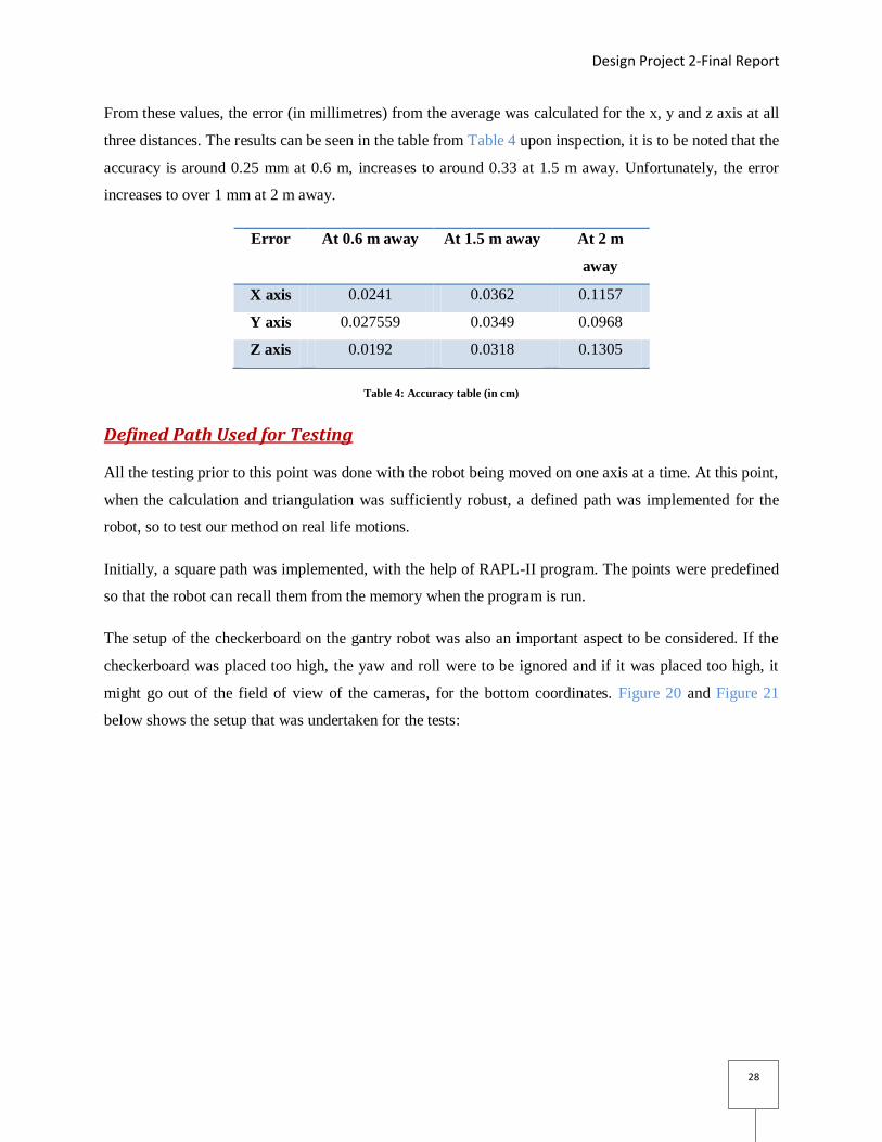
The setup of the checkerboard on the gantry robot was also an important aspect to be considered. If the
checkerboard was placed too high, the yaw and roll were to be ignored and if it was placed too high, it
might go out of the field of view of the cameras, for the bottom coordinates. Figure 20 and Figure 21
below shows the setup that was undertaken for the tests:
Design Project 2-Final Report
29
Figure 20: The Robot (before setup) Figure 21: The Robot (after Setup)
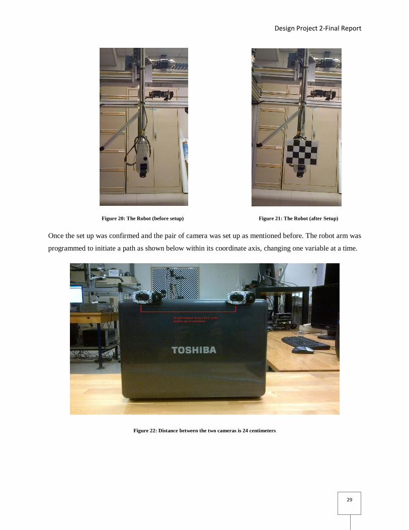
Once the set up was confirmed and the pair of camera was set up as mentioned before. The robot arm was
programmed to initiate a path as shown below within its coordinate axis, changing one variable at a time.
Figure 22: Distance between the two cameras is 24 centimeters
Design Project 2-Final Report
30
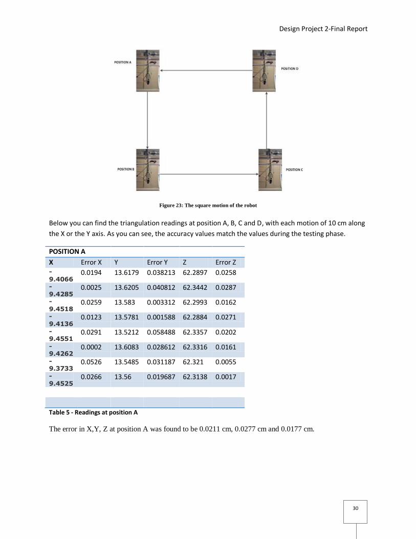
Figure 23: The square motion of the robot
Below you can find the triangulation readings at position A, B, C and D, with each motion of 10 cm along
the X or the Y axis. As you can see, the accuracy values match the values during the testing phase.
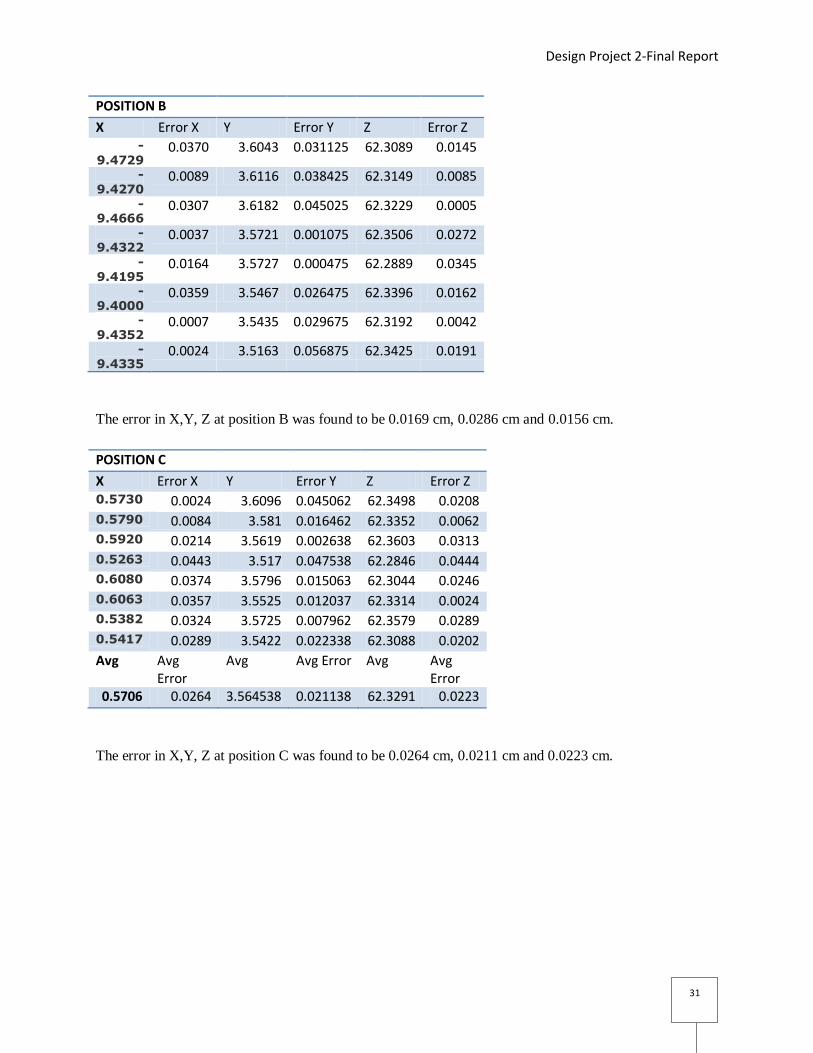
POSITION A
X Error X Y Error Y Z Error Z -9.4066
0.0194 13.6179 0.038213 62.2897 0.0258
-9.4285
0.0025 13.6205 0.040812 62.3442 0.0287
-9.4518
0.0259 13.583 0.003312 62.2993 0.0162
-9.4136
0.0123 13.5781 0.001588 62.2884 0.0271
-9.4551
0.0291 13.5212 0.058488 62.3357 0.0202
-9.4262
0.0002 13.6083 0.028612 62.3316 0.0161
-9.3733
0.0526 13.5485 0.031187 62.321 0.0055
-9.4525
0.0266 13.56 0.019687 62.3138 0.0017
Table 5 - Readings at position A
The error in X,Y, Z at position A was found to be 0.0211 cm, 0.0277 cm and 0.0177 cm.
Design Project 2-Final Report
31
POSITION B
X Error X Y Error Y Z Error Z -
9.4729 0.0370 3.6043 0.031125 62.3089 0.0145
-9.4270
0.0089 3.6116 0.038425 62.3149 0.0085
-9.4666
0.0307 3.6182 0.045025 62.3229 0.0005
-9.4322
0.0037 3.5721 0.001075 62.3506 0.0272
-9.4195
0.0164 3.5727 0.000475 62.2889 0.0345
-9.4000
0.0359 3.5467 0.026475 62.3396 0.0162
-9.4352
0.0007 3.5435 0.029675 62.3192 0.0042
-9.4335
0.0024 3.5163 0.056875 62.3425 0.0191
The error in X,Y, Z at position B was found to be 0.0169 cm, 0.0286 cm and 0.0156 cm.
POSITION C
X Error X Y Error Y Z Error Z 0.5730 0.0024 3.6096 0.045062 62.3498 0.0208 0.5790 0.0084 3.581 0.016462 62.3352 0.0062 0.5920 0.0214 3.5619 0.002638 62.3603 0.0313 0.5263 0.0443 3.517 0.047538 62.2846 0.0444 0.6080 0.0374 3.5796 0.015063 62.3044 0.0246 0.6063 0.0357 3.5525 0.012037 62.3314 0.0024 0.5382 0.0324 3.5725 0.007962 62.3579 0.0289 0.5417 0.0289 3.5422 0.022338 62.3088 0.0202
Avg Avg Error
Avg Avg Error Avg Avg Error
0.5706 0.0264 3.564538 0.021138 62.3291 0.0223
The error in X,Y, Z at position C was found to be 0.0264 cm, 0.0211 cm and 0.0223 cm.
Design Project 2-Final Report
32
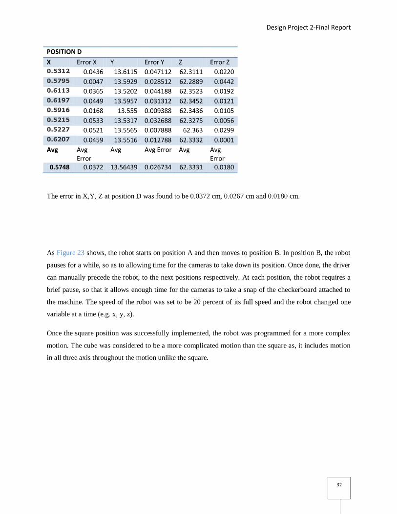
POSITION D
X Error X Y Error Y Z Error Z 0.5312 0.0436 13.6115 0.047112 62.3111 0.0220 0.5795 0.0047 13.5929 0.028512 62.2889 0.0442 0.6113 0.0365 13.5202 0.044188 62.3523 0.0192 0.6197 0.0449 13.5957 0.031312 62.3452 0.0121 0.5916 0.0168 13.555 0.009388 62.3436 0.0105 0.5215 0.0533 13.5317 0.032688 62.3275 0.0056 0.5227 0.0521 13.5565 0.007888 62.363 0.0299 0.6207 0.0459 13.5516 0.012788 62.3332 0.0001
Avg Avg Error
Avg Avg Error Avg Avg Error
0.5748 0.0372 13.56439 0.026734 62.3331 0.0180
The error in X,Y, Z at position D was found to be 0.0372 cm, 0.0267 cm and 0.0180 cm.
As Figure 23 shows, the robot starts on position A and then moves to position B. In position B, the robot
pauses for a while, so as to allowing time for the cameras to take down its position. Once done, the driver
can manually precede the robot, to the next positions respectively. At each position, the robot requires a
brief pause, so that it allows enough time for the cameras to take a snap of the checkerboard attached to
the machine. The speed of the robot was set to be 20 percent of its full speed and the robot changed one
variable at a time (e.g. x, y, z).
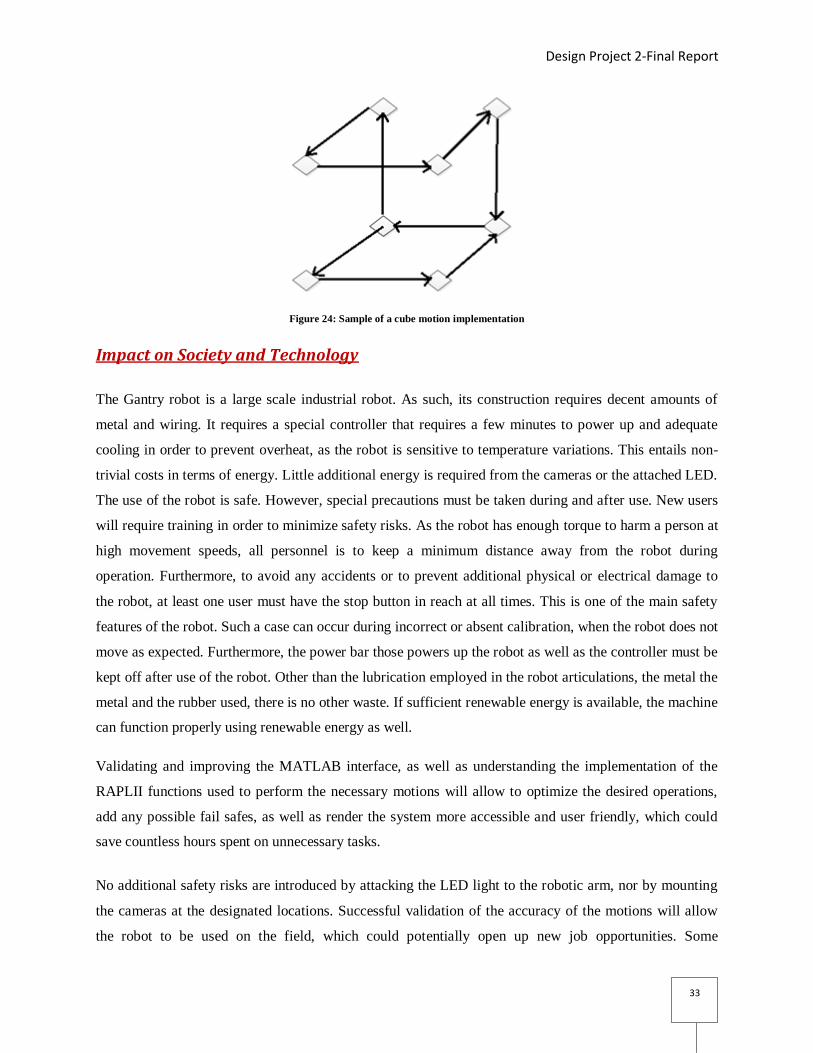
Once the square position was successfully implemented, the robot was programmed for a more complex
motion. The cube was considered to be a more complicated motion than the square as, it includes motion
in all three axis throughout the motion unlike the square.
Design Project 2-Final Report
33
Figure 24: Sample of a cube motion implementation
Impact on Society and Technology
The Gantry robot is a large scale industrial robot. As such, its construction requires decent amounts of
metal and wiring. It requires a special controller that requires a few minutes to power up and adequate
cooling in order to prevent overheat, as the robot is sensitive to temperature variations. This entails non-
trivial costs in terms of energy. Little additional energy is required from the cameras or the attached LED.
The use of the robot is safe. However, special precautions must be taken during and after use. New users
will require training in order to minimize safety risks. As the robot has enough torque to harm a person at
high movement speeds, all personnel is to keep a minimum distance away from the robot during
operation. Furthermore, to avoid any accidents or to prevent additional physical or electrical damage to
the robot, at least one user must have the stop button in reach at all times. This is one of the main safety
features of the robot. Such a case can occur during incorrect or absent calibration, when the robot does not
move as expected. Furthermore, the power bar those powers up the robot as well as the controller must be
kept off after use of the robot. Other than the lubrication employed in the robot articulations, the metal the
metal and the rubber used, there is no other waste. If sufficient renewable energy is available, the machine
can function properly using renewable energy as well.
Validating and improving the MATLAB interface, as well as understanding the implementation of the
RAPLII functions used to perform the necessary motions will allow to optimize the desired operations,
add any possible fail safes, as well as render the system more accessible and user friendly, which could
save countless hours spent on unnecessary tasks.
No additional safety risks are introduced by attacking the LED light to the robotic arm, nor by mounting
the cameras at the designated locations. Successful validation of the accuracy of the motions will allow
the robot to be used on the field, which could potentially open up new job opportunities. Some
Design Project 2-Final Report
34
applications include 3d data acquisition, assembly of various industrial parts using complex motions,
spray painting, manipulation of dangerous substances, among other, depending of the required accuracy
of the task.
Conclusion
Through research and practical experience on the task at hand, the team has learned about using the
Gantry robot and its specific programming language, about artificial perception techniques and devices. A
partial protocol capable of measuring the accuracy of simple spatial movements of the robot was
developed; this protocol includes the commands outputted in order to move the robot during
measurements, and the measuring tools and algorithms.
During the second part of the project, this protocol was be fine-tuned, tested and improved as required,
and more research was performed as new issues arose. Elaborate accuracy measurement software tools
were developed to perform image capture and find the triangulated world positions. These tools allowed
us to determine the accuracy of the position in world coordinates. The team was able to implement a
calibration code that was able to provide consistent results and also detect the gantry robot`s path and
coordinates within its boundaries after it moves. There is inconsistent behaviour near the edges of the
camera field of view. (results were found consistent for motions no longer than 10 cm). The team was not
able to fix it even though a plan was devised with the help of Professor Ferrie to fix this particular
problem, which can be found in Appendix 4.
If time would permit, we would mount a laser pointer instead of a chessboard pattern on the robot arm,
potentially allowing for more accurate position readings. Using the chessboard, another option would be
to also perform position readings across more complex, circular paths, and we would include code that
would calculate the pose of the robot arm as well as the position. Lastly, we would integrate our code
with the existing Matlab interface and have the code calculate the difference between the triangulated
position and the position taken as input before the motion is performed, as well as further enhance the
Matlab interface, as was initially planned.
Design Project 2-Final Report
35
References
1. http://www.wisegeek.com/what-are-gantry-robots.htm- Accessed on November 27, 2012
2. Dressler, Isolde. "Modeling and Control of Stiff Robots for Flexible Manufacturing.".
Department of Automatic Control Lund University, n.d. Web. 3 Dec 2012.
<http://www.control.lth.se/documents/2012/dressler2012phd.pdf>.
3. Smook, 0 .E.F.. "Camera Position Calibration Using the Image of Known Object Edges." . M.Sc.
Thesis, Measurement and Control Section ER, Department of Electrical Engineering, Eindhoven
University of Technology, 22 1994. Web. 3 Dec 2012.
<http://hanquier.m.free.fr/Worcester/references/Others papers/calibration/Camera Position
Calibration.pdf>.
4. http://www.vision.caltech.edu/bouguetj/calib_doc/htmls/parameters.html- Accessed on
November 27, 2012
5. http://www.umiacs.umd.edu/~ramani/cmsc828d/lecture9.pdf - Accessed on November 25, 2012
6. http://blog.martinperis.com/2011/08/stereo-vision-why-camera-calibration-is.html- Accessed on
November 25, 2012
7. http://www.vision.deis.unibo.it/smatt/Seminars/StereoVision.pdf - Accessed on November 25
8. http://www.wrotniak.net/photo/infrared/#DIFF- Accessed on December 4, 2012
9. http://www.vision.caltech.edu/bouguetj/calib_doc/ - Accessed on November 28, 2012
10. http://www.vision.caltech.edu/bouguetj/calib_doc/htmls/example5.html - Accessed on November
28, 2012
11. Emanuele Trucco and Alessandro Verri (1998). Introductory Techniques for 3-D Computer Vision.
Prentice Hall. ISBN 0-13-261108-2.
12. H. Christopher Longuet-Higgins (September 1981). "A computer algorithm for reconstructing a
scene from two projections". Nature 293 (5828): 133–135. doi:10.1038/293133a0.
Design Project 2-Final Report
36
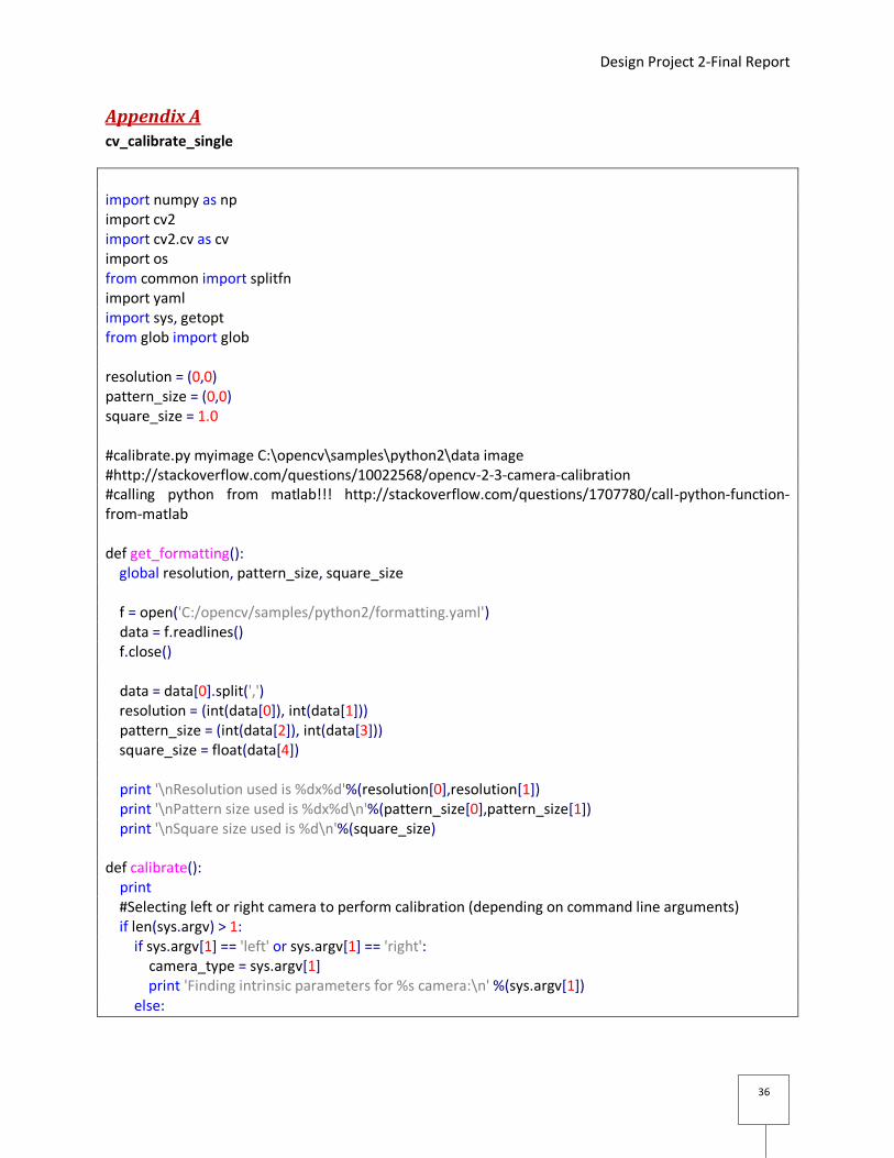
Appendix A cv_calibrate_single
import numpy as np import cv2 import cv2.cv as cv import os from common import splitfn import yaml import sys, getopt from glob import glob resolution = (0,0) pattern_size = (0,0) square_size = 1.0 #calibrate.py myimage C:\opencv\samples\python2\data image #http://stackoverflow.com/questions/10022568/opencv-2-3-camera-calibration #calling python from matlab!!! http://stackoverflow.com/questions/1707780/call-python-function-from-matlab def get_formatting(): global resolution, pattern_size, square_size f = open('C:/opencv/samples/python2/formatting.yaml') data = f.readlines() f.close() data = data[0].split(',') resolution = (int(data[0]), int(data[1])) pattern_size = (int(data[2]), int(data[3])) square_size = float(data[4]) print '\nResolution used is %dx%d'%(resolution[0],resolution[1]) print '\nPattern size used is %dx%d\n'%(pattern_size[0],pattern_size[1]) print '\nSquare size used is %d\n'%(square_size) def calibrate(): print #Selecting left or right camera to perform calibration (depending on command line arguments) if len(sys.argv) > 1: if sys.argv[1] == 'left' or sys.argv[1] == 'right': camera_type = sys.argv[1] print 'Finding intrinsic parameters for %s camera:\n' %(sys.argv[1]) else:
Design Project 2-Final Report
37
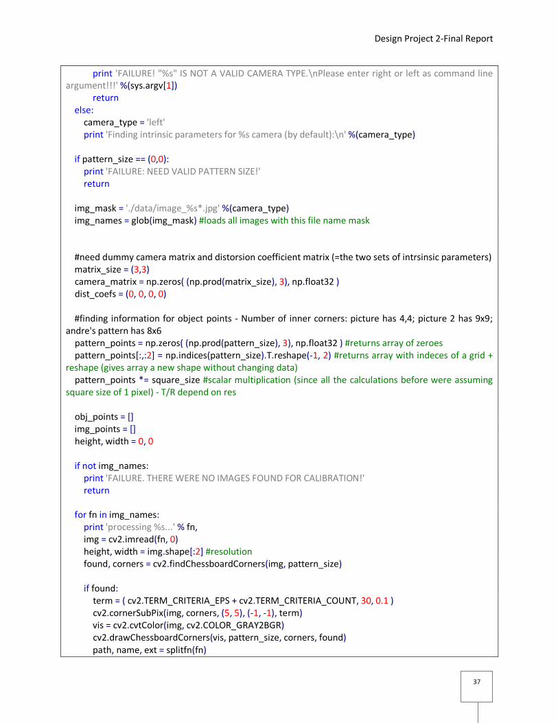
print 'FAILURE! "%s" IS NOT A VALID CAMERA TYPE.\nPlease enter right or left as command line argument!!!' %(sys.argv[1]) return else: camera_type = 'left' print 'Finding intrinsic parameters for %s camera (by default):\n' %(camera_type) if pattern_size == (0,0): print 'FAILURE: NEED VALID PATTERN SIZE!' return img_mask = './data/image_%s*.jpg' %(camera_type) img_names = glob(img_mask) #loads all images with this file name mask #need dummy camera matrix and distorsion coefficient matrix (=the two sets of intrsinsic parameters) matrix_size = (3,3) camera_matrix = np.zeros( (np.prod(matrix_size), 3), np.float32 ) dist_coefs = (0, 0, 0, 0) #finding information for object points - Number of inner corners: picture has 4,4; picture 2 has 9x9; andre's pattern has 8x6 pattern_points = np.zeros( (np.prod(pattern_size), 3), np.float32 ) #returns array of zeroes pattern_points[:,:2] = np.indices(pattern_size).T.reshape(-1, 2) #returns array with indeces of a grid + reshape (gives array a new shape without changing data) pattern_points *= square_size #scalar multiplication (since all the calculations before were assuming square size of 1 pixel) - T/R depend on res obj_points = [] img_points = [] height, width = 0, 0 if not img_names: print 'FAILURE. THERE WERE NO IMAGES FOUND FOR CALIBRATION!' return for fn in img_names: print 'processing %s...' % fn, img = cv2.imread(fn, 0) height, width = img.shape[:2] #resolution found, corners = cv2.findChessboardCorners(img, pattern_size) if found: term = ( cv2.TERM_CRITERIA_EPS + cv2.TERM_CRITERIA_COUNT, 30, 0.1 ) cv2.cornerSubPix(img, corners, (5, 5), (-1, -1), term) vis = cv2.cvtColor(img, cv2.COLOR_GRAY2BGR) cv2.drawChessboardCorners(vis, pattern_size, corners, found) path, name, ext = splitfn(fn)
Design Project 2-Final Report
38
cv2.imwrite('./debug/%s_chess.jpg'%(name), vis) if not found: print 'chessboard not found' continue img_points.append(corners.reshape(-1, 2)) obj_points.append(pattern_points) print 'ok' #calculate camera matrix and dist coeff rms, camera_matrix, dist_coefs, rvecs, tvecs = cv2.calibrateCamera(obj_points, img_points, (width, height), camera_matrix, dist_coefs) print "\nRMS:", rms #final reprojection error print "camera matrix:\n", camera_matrix #you need only 00, 02, 11, 12 print "distortion coefficients:\n ", dist_coefs.ravel() #ravel flattens matrix cv2.destroyAllWindows() #calculate and display some important parameters fovx, fovy, focalLength, principalPoint, aspectRatio = cv2.calibrationMatrixValues(camera_matrix, resolution, 1, 1) print "\nField of view over X:", fovx print "Field of view over Y:", fovy print "Focal length", focalLength print "Principal point:", principalPoint print "Aspect ratio:", aspectRatio, "\n" #writing intrinsic parameters to yaml file (basically text file) #first 4 values are fx, cx, fy, cy; next 5 values are the distorsion coefficients cv.Save('C:/opencv/samples/python2/intrinsic_camera_%s.yaml'%(camera_type), cv.fromarray(camera_matrix)) cv.Save('C:/opencv/samples/python2/intrinsic_distorsion_%s.yaml'%(camera_type), cv.fromarray(dist_coefs)) return def main(): get_formatting() calibrate() return if __name__ == "__main__": main()
Design Project 2-Final Report
39
cv_calibrate_stereo
import numpy as np import cv2 import cv2.cv as cv import os from common import splitfn import yaml import sys, getopt from glob import glob import csv resolution = (0,0) pattern_size = (0,0) square_size = 1.0 def get_formatting(): global resolution, pattern_size, square_size f = open('C:/opencv/samples/python2/formatting.yaml') data = f.readlines() f.close() data = data[0].split(',') resolution = (int(data[0]), int(data[1])) pattern_size = (int(data[2]), int(data[3])) square_size = float(data[4]) print '\nResolution used is %dx%d'%(resolution[0],resolution[1]) print '\nPattern size used is %dx%d\n'%(pattern_size[0],pattern_size[1]) print '\nSquare size used is %f\n'%(square_size) def get_intrinsic(camera_type): #loading intrinsic parameters from file #first 4 values are fx, cx, fy, cy - next 5 values are the distorsion coefficients if camera_type == 'left' or camera_type == 'right': print 'Acquiring intrinsic parameters for %s camera from file.' %(camera_type) else: print 'FAILURE: Camera type cannot be %s' %(camera_type) return try: camera_matrix = np.asarray(cv.Load('C:/opencv/samples/python2/intrinsic_camera_%s.yaml'%(camera_type), cv.CreateMemStorage()))
Design Project 2-Final Report
40
dist_coefs = np.asarray(cv.Load('C:/opencv/samples/python2/intrinsic_distorsion_%s.yaml'%(camera_type), cv.CreateMemStorage())) return camera_matrix, dist_coefs except IOError: print "EXCEPTION: File was not found or could not be read." return def find_chessboard(camera_type, img_points, obj_points): if camera_type == 'left' or camera_type == 'right': print 'Acquiring image points and object points for the %s camera.' %(camera_type) else: print 'FAILURE: Camera type cannot be %s' %(camera_type) return #print pattern_size if pattern_size == (0,0): print 'FAILURE: NEED VALID PATTERN SIZE!' return img_mask = './data/image_%s*.jpg' %(camera_type) img_names = glob(img_mask) #loads all images with this file name mask #2.7 #1.0 #need dummy camera matrix and distorsion coefficient matrix (=the two sets of intrsinsic parameters) matrix_size = (3,3) camera_matrix = np.zeros( (np.prod(matrix_size), 3), np.float32 ) dist_coefs = (0, 0, 0, 0) #finding information for object points - Number of inner corners: picture has 4,4; picture 2 has 9x9; andre's pattern has 8x6 pattern_points = np.zeros( (np.prod(pattern_size), 3), np.float32 ) #returns array of zeroes pattern_points[:,:2] = np.indices(pattern_size).T.reshape(-1, 2) #returns array with indeces of a grid + reshape (gives array a new shape without changing data) pattern_points *= square_size #scalar multiplication (since all the calculations before were assuming square size of 1 pixel) - T/R depend on res height, width = 0, 0 if not img_names: print 'FAILURE. THERE WERE NO IMAGES FOUND FOR CALIBRATION!' return for fn in img_names: #print 'processing %s...' % fn, img = cv2.imread(fn, 0) height, width = img.shape[:2] #resolution
Design Project 2-Final Report
41
found, corners = cv2.findChessboardCorners(img, pattern_size) if found: term = ( cv2.TERM_CRITERIA_EPS + cv2.TERM_CRITERIA_COUNT, 30, 0.1 ) cv2.cornerSubPix(img, corners, (5, 5), (-1, -1), term) if not found: print 'chessboard not found' continue img_points.append(corners.reshape(-1, 2)) obj_points.append(pattern_points) #print 'ok' return def calibrate_stereo(): #if this doesn't work, use CreateMat(rows, cols, type) -> mat to recreate matrix !!! type is F for float #http://opencv.willowgarage.com/documentation/python/calib3d_camera_calibration_and_3d_reconstruction.html print img_points_left = [] img_points_right = [] obj_points_left = [] obj_points_right = [] #same as left #reading intrinsic parameters from file camera_matrix_left, dist_coefs_left = get_intrinsic('left') camera_matrix_right, dist_coefs_right = get_intrinsic('right') print camera_matrix_left, '\n\n', camera_matrix_right, '\n\n', dist_coefs_left, '\n\n', dist_coefs_right, '\n\n' #obtaining object points and image points find_chessboard('left', img_points_left, obj_points_left) find_chessboard('right', img_points_right, obj_points_right) #stereo calibration (finding translation and rotation vector of right camera onto the left one rms, cm1, dc1, cm2, dc2, rotation, translation, E, fundM = cv2.stereoCalibrate(obj_points_left, img_points_left, img_points_right, resolution, \ camera_matrix_left, dist_coefs_left, camera_matrix_right, dist_coefs_right, flags = 1) print print 'Translation matrix of right camera onto left camera is:\n', translation print 'Rotation matrix of right camera onto left camera is:\n', rotation
Design Project 2-Final Report
42
#saving translation and rotation vector to file cv.Save('C:/opencv/samples/python2/extrinsic_translation.yaml', cv.fromarray(translation)) cv.Save('C:/opencv/samples/python2/extrinsic_rotation.yaml', cv.fromarray(rotation)) R1 = cv.CreateMat(3, 3, cv.CV_64FC1) #must be double!!!! R2 = cv.CreateMat(3, 3, cv.CV_64FC1) P1 = cv.CreateMat(3, 4, cv.CV_64FC1) P2 = cv.CreateMat(3, 4, cv.CV_64FC1) Q = cv.CreateMat(4, 4, cv.CV_64FC1) print '\nPerforming the stereo rectification' cv.StereoRectify(cv.fromarray(camera_matrix_left), cv.fromarray(camera_matrix_right), cv.fromarray(dist_coefs_left), cv.fromarray(dist_coefs_right), \ resolution, cv.fromarray(rotation), cv.fromarray(translation), R1, R2, P1, P2, Q, alpha=-1, newImageSize=(0, 0)) P1 = np.asarray(P1) P2 = np.asarray(P2) print print '\nProjection matrix for left image:\n', P1 print 'Projection matrix for right image:\n', P2 #USE THIS IF YOU DECIDE TO CREATE SEPARATE TRIANGULATION THAT YOU LOOP THROUGH - saving projection matrices to file cv.Save('C:/opencv/samples/python2/proj_matrix_left.yaml', cv.fromarray(P1)) cv.Save('C:/opencv/samples/python2/proj_matrix_right.yaml', cv.fromarray(P2)) cv.Save('C:/opencv/samples/python2/fund_matrix.yaml', cv.fromarray(fundM)) def main(): get_formatting() #gets resolution and pattern size from file print resolution print pattern_size calibrate_stereo() return if __name__ == "__main__": main()
cv_calibrate_stereo import numpy as np
Design Project 2-Final Report
43
import cv2 import cv2.cv as cv import os from common import splitfn import yaml import sys, getopt from glob import glob import csv import winsound #http://tech.groups.yahoo.com/group/OpenCV/message/81443 #https://code.ros.org/trac/opencv/ticket/1319 #http://stackoverflow.com/questions/1707780/call-python-function-from-matlab resolution = (0,0) pattern_size = (0,0) square_size = 1.0 def get_formatting(): global resolution, pattern_size, square_size f = open('C:/opencv/samples/python2/formatting.yaml') data = f.readlines() f.close() data = data[0].split(',') resolution = (int(data[0]), int(data[1])) pattern_size = (int(data[2]), int(data[3])) square_size = float(data[4]) print data[4] print float(data[4]) print square_size print '\nResolution used is %dx%d'%(resolution[0],resolution[1]) print '\nPattern size used is %dx%d\n'%(pattern_size[0],pattern_size[1]) print '\nSquare size used is %f\n'%(square_size) def get_intrinsic(camera_type): #loading intrinsic parameters from file #first 4 values are fx, cx, fy, cy - next 5 values are the distorsion coefficients if camera_type == 'left' or camera_type == 'right': print 'Acquiring intrinsic parameters for %s camera from file.' %(camera_type) else: print 'FAILURE: Camera type cannot be %s' %(camera_type) return
Design Project 2-Final Report
44
try: camera_matrix = np.asarray(cv.Load('C:/opencv/samples/python2/intrinsic_camera_%s.yaml'%(camera_type), cv.CreateMemStorage())) dist_coefs = np.asarray(cv.Load('C:/opencv/samples/python2/intrinsic_distorsion_%s.yaml'%(camera_type), cv.CreateMemStorage())) return camera_matrix, dist_coefs except IOError: print "EXCEPTION: File was not found or could not be read." return def take_projection_point_picture(camera_type): index = 0 if camera_type == 'left': camera = cv.CaptureFromCAM(0) #left cam ---FIND CORRECT VALUES elif camera_type == 'right': camera = cv.CaptureFromCAM(1) #right cam else: print 'FAILURE: Invalid camera type!' return cv.SetCaptureProperty(camera, cv.CV_CAP_PROP_FRAME_WIDTH, resolution[0]) cv.SetCaptureProperty(camera, cv.CV_CAP_PROP_FRAME_HEIGHT, resolution[1]) print '\nAcquiring images at %sx%s resolution!\n' %(resolution[0], resolution[1]) print 'WHEN YOU HEAR THE BEEP, MUST STAND STILL\n' image = cv.QueryFrame(camera) cv.SaveImage(".\data\proj_point_image_%s.jpg"%(camera_type), image) print '\nSaved %s projection point image into the .\data folder!'%(camera_type) def find_proj_points(camera_type, img_points): if camera_type == 'left' or camera_type == 'right': print '\nAcquiring projection points for the %s camera.' %(camera_type) else: print 'FAILURE: Camera type cannot be %s' %(camera_type) return #reading saved projection point image from file img_mask = './data/proj_point_image_%s*.jpg' %(camera_type) img_names = glob(img_mask) #loads all images with this file name mask
Design Project 2-Final Report
45
#need dummy camera matrix and distorsion coefficient matrix (=the two sets of intrsinsic parameters) matrix_size = (3,3) camera_matrix = np.zeros( (np.prod(matrix_size), 3), np.float32 ) dist_coefs = (0, 0, 0, 0) #finding information for object points - Number of inner corners: picture has 4,4; picture 2 has 9x9; andre's pattern has 8x6 height, width = 0, 0 if not img_names: print 'FAILURE. THERE WERE NO IMAGES FOUND FOR CALIBRATION!' sys.exit() #finding projection points (=chessboard points) from image fn = img_names[0] #print 'processing %s...' % fn, img = cv2.imread(fn, 0) height, width = img.shape[:2] #resolution found, corners = cv2.findChessboardCorners(img, pattern_size) img_index = 0 #drawing chessboard points to image and saving image if found: term = ( cv2.TERM_CRITERIA_EPS + cv2.TERM_CRITERIA_COUNT, 30, 0.1 ) cv2.cornerSubPix(img, corners, (5, 5), (-1, -1), term) img_mask = './debug/proj_point_%s_chess*.jpg'%(camera_type) img_names = glob(img_mask) #loads all images with this file name mask img_index = len(img_names) vis = cv2.cvtColor(img, cv2.COLOR_GRAY2BGR) cv2.drawChessboardCorners(vis, pattern_size, corners, found) #path, name, ext = splitfn(fn) cv2.imwrite('./debug/proj_point_%s_chess_%d.jpg'%(camera_type, img_index), vis) if not found: print 'Chessboard not found. One of the camera might have its view blocked.' sys.exit() img_points.append(corners.reshape(-1, 2)) return img_points def triangulate_all_points(proj_matrix_1, proj_matrix_2, fundM): proj_points_left = [] proj_points_right = [] print '\a', '\a', '\a' # 3 beeping noises STAND STILL
Design Project 2-Final Report
46
#taking pictures for projection points take_projection_point_picture('left') take_projection_point_picture('right') #acquiring projection points find_proj_points('left', proj_points_left) find_proj_points('right', proj_points_right) proj_points_left = np.asarray(proj_points_left) #take only 1 or many projection points??? proj_points_right = np.asarray(proj_points_right) #refines coordinates of corresponding points print '\nFirst point of left camera projection points BEFORE correct_matches:\n', proj_points_left[0][0], '\n' proj_points_left, proj_points_right= cv2.correctMatches(fundM, proj_points_left, proj_points_right) print 'First point of left camera projection points AFTER correct_matches:\n', proj_points_left[0][0], '\n' #triangulates 3d position points4D = cv2.triangulatePoints(proj_matrix_1, proj_matrix_2, proj_points_left, proj_points_right) #do proj points need to be homogenous ??? ''' #using convertToNonHom() points4D = points4D.reshape(np.prod(pattern_size), 4) points4D = cv2.convertPointsFromHomogeneous(points4D) points4D = np.asarray(points4D) first_point = ( float(points4D[0][0][0]), float(points4D[0][0][1]), float(points4D[0][0][2]) ) ''' #turning matrix into non-homogenous (euclidean) points4D /= points4D[3] first_point = (points4D[0][0], points4D[1][0], points4D[2][0]) print '\nNew point is:',first_point, '\n' #saving point to csv with open("output.csv", "ab") as f: fileWriter = csv.writer(f, delimiter=',',quotechar='|', quoting=csv.QUOTE_MINIMAL) fileWriter.writerow(first_point) return first_point def main(): '''Function that triangulates 3d world coordinate of the first point of a chessboard from intrinsic and extrinsic parameters, saves the point to a csv file, and performs the difference between the old point and the new point '''
Design Project 2-Final Report
47
#read current resolution, pattern size and square size get_formatting() #gets resolution and pattern size from file #load projection and fundamental matrices from file (needed for triangulation) P1 = np.asarray(cv.Load('C:/opencv/samples/python2/proj_matrix_left.yaml', cv.CreateMemStorage())) P2 = np.asarray(cv.Load('C:/opencv/samples/python2/proj_matrix_right.yaml', cv.CreateMemStorage())) fundM = np.asarray(cv.Load('C:/opencv/samples/python2/fund_matrix.yaml', cv.CreateMemStorage())) #clear the .csv file if there is 'cl' command line argument argc = len(sys.argv) if argc == 2: if sys.argv[1] == 'cl': f = open('output.csv', "w") f.truncate() f.close() print '\nCLEARED output.csv FILE\n' new_point, old_point = (0, 0, 0), (0, 0, 0) difference = (0, 0, 0) length = 0 #triangulate new_point = triangulate_all_points(P1, P2, fundM) file = os.getcwd() file = os.path.join(file, "output.csv") #getting # of rows of .csv file with open(file, 'rb') as csvfile: spamreader = csv.reader(csvfile, delimiter=',', quotechar='|') index = 0 for row in spamreader: length = length + 1 #Read first point from csv file and perform difference between new point and previous point with open(file, 'rb') as csvfile: spamreader = csv.reader(csvfile, delimiter=',', quotechar='|') index = 0
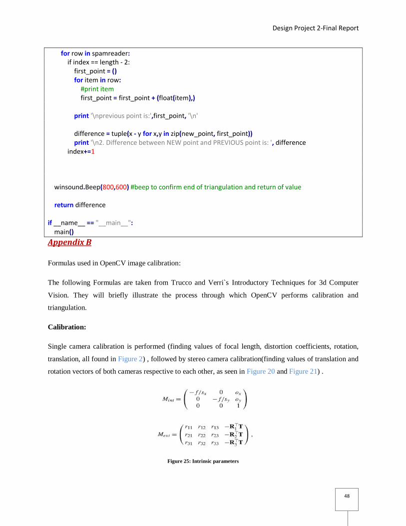
Design Project 2-Final Report
48
for row in spamreader: if index == length - 2: first_point = () for item in row: #print item first_point = first_point + (float(item),) print '\nprevious point is:',first_point, '\n' difference = tuple(x - y for x,y in zip(new_point, first_point)) print '\n2. Difference between NEW point and PREVIOUS point is: ', difference index+=1 winsound.Beep(800,600) #beep to confirm end of triangulation and return of value return difference if __name__ == "__main__": main()
Appendix B
Formulas used in OpenCV image calibration:
The following Formulas are taken from Trucco and Verri`s Introductory Techniques for 3d Computer
Vision. They will briefly illustrate the process through which OpenCV performs calibration and
triangulation.
Calibration:
Single camera calibration is performed (finding values of focal length, distortion coefficients, rotation,
translation, all found in Figure 2) , followed by stereo camera calibration(finding values of translation and
rotation vectors of both cameras respective to each other, as seen in Figure 20 and Figure 21) .
Figure 25: Intrinsic parameters
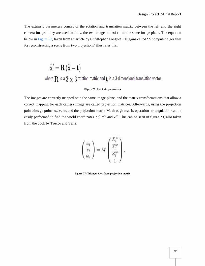
Design Project 2-Final Report
49
The extrinsic parameters consist of the rotation and translation matrix between the left and the right
camera images: they are used to allow the two images to exist into the same image plane. The equation
below in Figure 22, taken from an article by Christopher Longuet – Higgins called ‘A computer algorithm
for reconstructing a scene from two projections’ illustrates this.
Figure 26: Extrinsic parameters
The images are correctly mapped onto the same image plane, and the matrix transformations that allow a
correct mapping for each camera image are called projection matrices. Afterwards, using the projection
points/image points ui, vi, wi and the projection matrix M, through matrix operations triangulation can be
easily performed to find the world coordinates Xw, Y
w and Z
w. This can be seen in figure 23, also taken
from the book by Trucco and Verri.
Figure 27: Triangulation from projection matrix
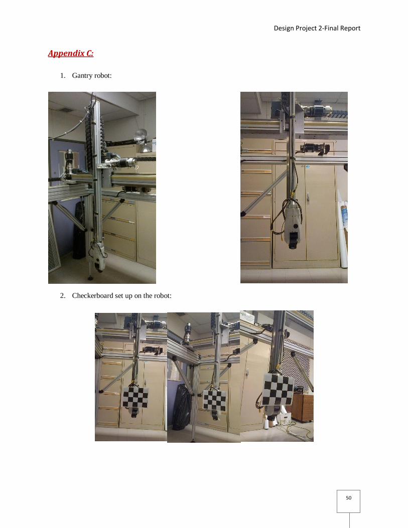
Design Project 2-Final Report
50
Appendix C:
1. Gantry robot:
2. Checkerboard set up on the robot:
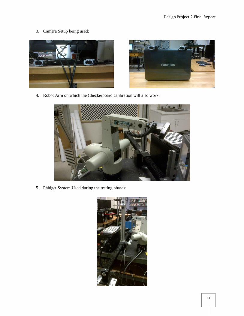
Design Project 2-Final Report
51
3. Camera Setup being used:
4. Robot Arm on which the Checkerboard calibration will also work:
5. Phidget System Used during the testing phases:
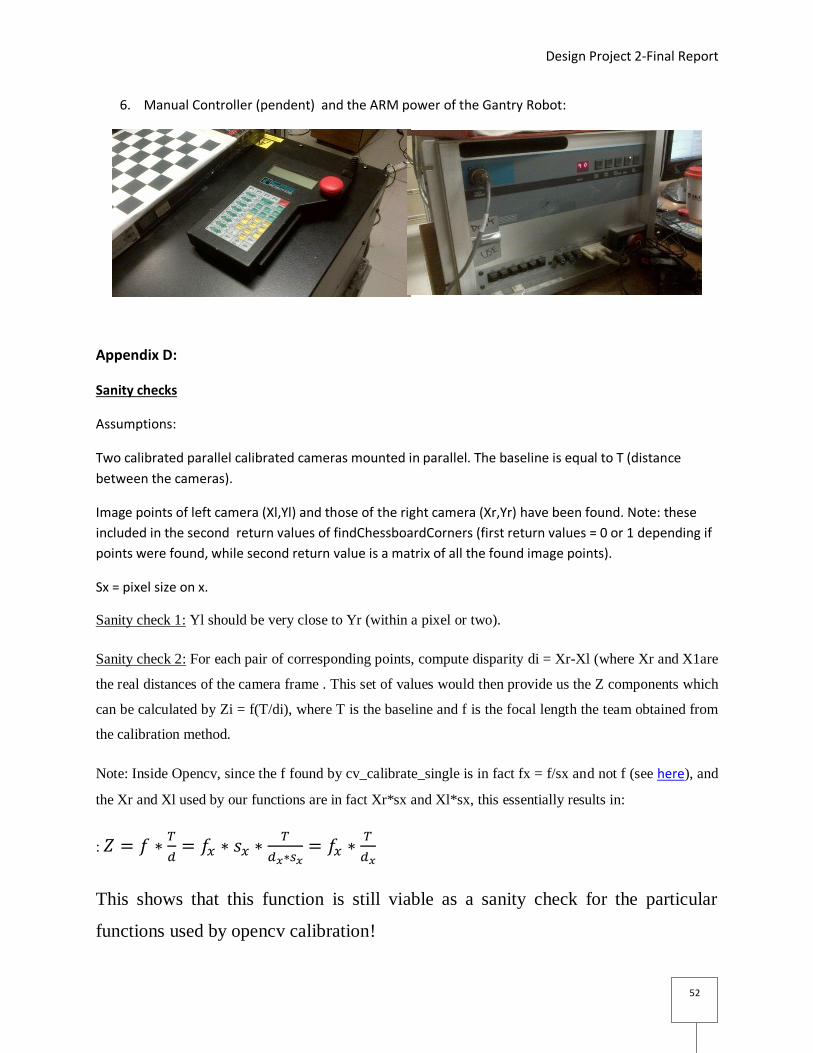
Design Project 2-Final Report
52
6. Manual Controller (pendent) and the ARM power of the Gantry Robot:
Appendix D:
Sanity checks
Assumptions:
Two calibrated parallel calibrated cameras mounted in parallel. The baseline is equal to T (distance
between the cameras).
Image points of left camera (Xl,Yl) and those of the right camera (Xr,Yr) have been found. Note: these
included in the second return values of findChessboardCorners (first return values = 0 or 1 depending if
points were found, while second return value is a matrix of all the found image points).
Sx = pixel size on x.
Sanity check 1: Yl should be very close to Yr (within a pixel or two).
Sanity check 2: For each pair of corresponding points, compute disparity di = Xr-Xl (where Xr and X1are
the real distances of the camera frame . This set of values would then provide us the Z components which
can be calculated by Zi = f(T/di), where T is the baseline and f is the focal length the team obtained from
the calibration method.
Note: Inside Opencv, since the f found by cv_calibrate_single is in fact fx = f/sx and not f (see here), and
the Xr and Xl used by our functions are in fact Xr*sx and Xl*sx, this essentially results in:
:
This shows that this function is still viable as a sanity check for the particular
functions used by opencv calibration!