1

ECS231

Uniprocessor Optimization of Matrix Multiplications and BLAS

For an extended discussion, see Berkeley CS267 Lecture on ``Single Processor

Machines: Memory Hierarchies and Processor Features’’ by J. Demmel

2

Outline

1. Memory Hierarchies

2. Cache and its importance in performance

3. Optimizing matrix multiply for caches

4. BLAS

5. Optimization in practice

6. Supplement: Strassen’s algorithm

3

Memory Hierarchy

• Most programs have a high degree of locality in their accesses

• spatial locality: accessing things nearby previous accesses

• temporal locality: reusing an item that was previously accessed

• Memory hierarchy tries to exploit locality

• By taking advantage of the principle of locality:

• present the user with as much memory as is available in the cheapest technology

• Provide access at the speed offered by the fastest technology

4

Memory Hierarchy

Control

Datapath

Secondary

Storage

(Disk)

Processor

Reg

isters

Main

Memory

(DRAM)

Second

Level

Cache

(SRAM)

On

-Ch

ip

Ca

che

1s 10,000,000s

(10s ms)

Speed (ns): 10s 100s

100s Gs Size (bytes): Ks Ms

Tertiary

Storage

(Disk/Tape)

10,000,000,000s

(10s sec)

Ts

5

Levels of the Memory Hierarchy

CPU Registers 100s Bytes <10s ns

Cache K Bytes 10-100 ns 1-0.1 cents/bit

Main Memory M Bytes 200ns- 500ns $.0001-.00001 cents /bit

Disk G Bytes, 10 ms (10,000,000 ns) 10 - 10 cents/bit

-5 -6

Capacity Access Time Cost

Tape infinite sec-min 10 -8

Registers

Cache

Memory

Disk / Distributed Memory

Tape / Clusters

Instr. Operands

Blocks

Pages

Files

Staging Xfer Unit

prog./compiler 1-8 bytes

cache cntl 8-128 bytes

OS 512-4K bytes

user/operator Mbytes

Upper Level

Lower Level

faster

Larger

6

Idealized Uniprocessor Model

• Processor names bytes, words, etc. in its address space

• These represent integers, floats, pointers, arrays, etc.

• Exist in the program stack, static region, or heap

• Operations include

• Read and write (given an address/pointer)

• Arithmetic and other logical operations

• Order specified by program

• Read returns the most recently written data

• Compiler and architecture translate high level expressions into “obvious” lower level instructions

• Hardware executes instructions in order specified by compiler

• Cost

• Each operations has roughly the same cost (read, write, add, multiply, etc.)

7

Uniprocessors in the Real World

• Real processors have • registers and caches

• small amounts of fast memory

• store values of recently used or nearby data

• different memory ops can have very different costs

• parallelism

• multiple “functional units” that can run in parallel

• different orders, instruction mixes have different costs

• pipelining

• a form of parallelism, like an assembly line in a factory

• Why is this your problem? In theory, compilers understand all of this and can

optimize your program; in practice they don’t.

8

Processor-DRAM Gap (latency)

µProc

60%/yr.

DRAM

7%/yr. 1

10

100

1000

1980

1981

1983

1984

1985

1986

1987

1988

1989

1990

1991

1992

1993

1994

1995

1996

1997

1998

1999

2000

DRAM

CPU 1982

Processor-Memory

Performance Gap:

(grows 50% / year)

Perf

orm

an

ce

Time

“Moore’s Law”

• Memory hierarchies are getting deeper

• Processors get faster more quickly than memory

9

Matrix-multiply, optimized several ways

Speed of n-by-n matrix multiply on Sun Ultra-1/170, peak = 330 MFlops

10

Cache and Its Importance in Performance

• Motivation:

• Time to run code = clock cycles running code

+ clock cycles waiting for memory

• For many years, CPU’s have sped up an average of 50% per year over memory chip speed ups.

• Hence, memory access is computing the bottleneck. The computational cost of an algorithm can already exceed arithmetic cost by orders of magnitude, and the gap is growing.

• Ref: Graham, Snior and Patterson, ``Getting up to speed: the future of supercomputing’’, National Academies Press, 2005.

11

Cache Benefits

• Data cache was designed with two key concepts in mind

• Spatial Locality

• When an element is referenced its neighbors will be referenced too

• Cache lines are fetched together

• Work on consecutive data elements in the same cache line

• Temporal Locality

• When an element is referenced, it might be referenced again soon

• Arrange code so that data in cache is reused often

12

Lessons

• Actual performance of a simple program can be a

complicated function of the architecture

• Slight changes in the architecture or program change the

performance significantly

• To write fast programs, need to consider architecture

• We would like simple models to help us design efficient

algorithms

• Is this possible?

• We will illustrate with a common technique for improving

cache performance, called blocking or tiling

• Basic idea: used divide-and-conquer to define a problem that

fits in register/L1-cache/L2-cache

13

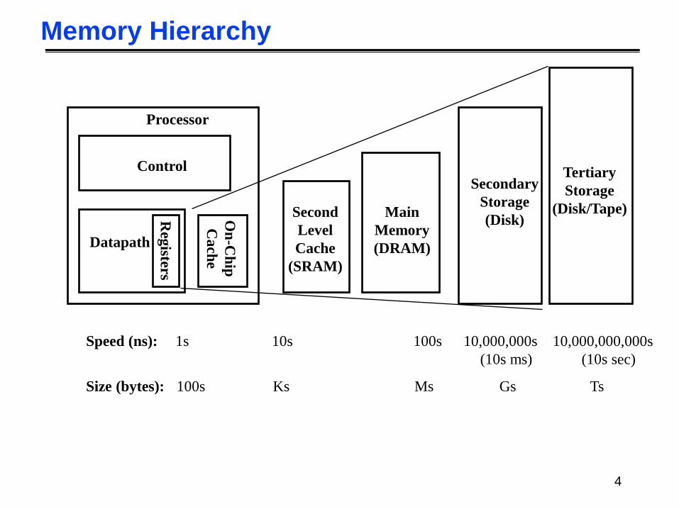
Note on Matrix Storage

• A matrix is a 2-D array of elements, but memory addresses are “1-D”

• Conventions for matrix layout

• by column, or “column major” (Fortran default)

• by row, or “row major” (C default)

0

1

2

3

4

5

6

7

8

9

10

11

12

13

14

15

16

17

18

19

0

4

8

12

16

1

5

9

13

17

2

6

10

14

18

3

7

11

15

19

Column major Row major

14

• Assume just 2 levels in the hierarchy, fast and slow

• All data initially in slow memory

• m = number of memory elements (words) moved between fast and slow memory

• tm = time per slow memory operation

• f = number of arithmetic operations

• tf = time per arithmetic operation << tm

• q = f / m average number of flops per slow element access

• Minimum possible time = f* tf when all data in fast memory

• Total time

• Larger q means Total time closer to minimum f * tf

Using a Simple Model of Memory to Optimize

Key to

algorithm

efficiency

f * tf + m * tm = f * tf * (1 + tm/tf * 1/q) Key to

machine

efficiency

15

Warm up: Matrix-vector multiplication

{implements y = y + A*x}

for i = 1:n

for j = 1:n

y(i) = y(i) + A(i,j)*x(j)

= + *

y(i) y(i)

A(i,:)

x(:)

16

Warm up: Matrix-vector multiplication

{read x(1:n) into fast memory}

{read y(1:n) into fast memory}

for i = 1:n

{read row i of A into fast memory}

for j = 1:n

y(i) = y(i) + A(i,j)*x(j)

{write y(1:n) back to slow memory}

• m = number of slow memory refs = 3n + n2

• f = number of arithmetic operations = 2n2

• q = f / m ~= 2

• Matrix-vector multiplication limited by slow memory speed

17

“Naïve” Matrix Multiply

{implements C = C + A*B}

for i = 1 to n

for j = 1 to n

for k = 1 to n

C(i,j) = C(i,j) + A(i,k) * B(k,j)

= + *

C(i,j) C(i,j) A(i,:)

B(:,j)

18

“Naïve” Matrix Multiply

{implements C = C + A*B}

for i = 1 to n

{read row i of A into fast memory}

for j = 1 to n

{read C(i,j) into fast memory}

{read column j of B into fast memory}

for k = 1 to n

C(i,j) = C(i,j) + A(i,k) * B(k,j)

{write C(i,j) back to slow memory}

= + *

C(i,j) A(i,:)

B(:,j)

C(i,j)

19

“Naïve” Matrix Multiply

Number of slow memory references on unblocked matrix multiply

m = n3 read each column of B n times

+ n2 read each row of A once

+ 2n2 read and write each element of C once

= n3 + 3n2

Therefore

q = f / m = 2n3 / (n3 + 3n2) ~= 2 for large n,

No improvement over matrix-vector multiply!

= + *

C(i,j) C(i,j) A(i,:)

B(:,j)

20

Blocked (Tiled) Matrix Multiply

Consider A,B,C to be N by N matrices of b by b subblocks where b=n / N is called the block size

for i = 1 to N

for j = 1 to N

{read block C(i,j) into fast memory}

for k = 1 to N

{read block A(i,k) into fast memory}

{read block B(k,j) into fast memory}

C(i,j) = C(i,j) + A(i,k) * B(k,j) {do a matrix multiply on blocks}

{write block C(i,j) back to slow memory}

= + *

C(i,j) C(i,j) A(i,k)

B(k,j)

21

Blocked (Tiled) Matrix Multiply

Recall:

m is amount memory traffic between slow and fast memory

matrix has nxn elements, and NxN blocks, each of size bxb

f is number of floating point operations, f = 2n3

q = f / m: measure of algorithm efficiency in the memory system

The amount of memory traffic is

m = N*n2 read each block of B N3 times (N3 * n/N * n/N)

+ N*n2 read each block of A N3 times

+ 2n2 read and write each block of C once

= (2N + 2) * n2

Therefore

q = f / m = 2n3 / ((2N + 2) * n2) ~= n / N = b for large n

Hence we can improve performance by increasing the blocksize b.

22

Limits to Optimizing Matrix Multiply

The blocked algorithm has ratio q ~= b

• The large the block size, the more efficient our algorithm will be

• Limit: All three blocks from A,B,C must fit in fast memory (cache),

so we cannot make these blocks arbitrarily large:

3b2 <= M, so q ~= b <= sqrt(M/3)

There is a lower bound result:

Theorem (Hong & Kung, 1981): Any reorganization of this algorithm

(that uses only algebraic associativity) is limited to q = O(sqrt(M))

23

Fast linear algebra kernels: BLAS

• Simple linear algebra kernels such as matrix-matrix multiply

• More complicated algorithms can be built from these basic kernels.

• The interfaces of these kernels have been standardized as the Basic Linear Algebra Subroutines (BLAS).

• Early agreement on standard interface (~1980)

• Led to portable libraries for vector and shared memory parallel machines.

• On distributed memory, there is a less-standard interface called the PBLAS

24

BLAS: advantages

• Clarity: code is shorter and easier to read,

• Modularity: gives programmer larger building blocks,

• Performance: manufacturers will provide tuned machine-specific BLAS,

• Program portability: machine dependencies are confined to the BLAS

25

Basic Linear Algebra Subroutines

• History

• BLAS1 (1970s):

• vector operations: dot product, saxpy (y=a*x+y), etc

• m=2*n, f=2*n, q ~1 or less

• BLAS2 (mid 1980s)

• matrix-vector operations: matrix vector multiply, etc

• m=n^2, f=2*n^2, q~2, less overhead

• somewhat faster than BLAS1

• BLAS3 (late 1980s)

• matrix-matrix operations: matrix matrix multiply, etc

• m >= 4n^2, f=O(n^3), so q can possibly be as large as n, so BLAS3 is potentially much faster than BLAS2

• Good algorithms used BLAS3 when possible (e.g., LAPACK)

• See www.netlib.org/blas, www.netlib.org/lapack

26

Level 1, 2 and 3 BLAS

• Level 1 BLAS Vector-Vector operations

• Level 2 BLAS Matrix-Vector operations

• Level 3 BLAS Matrix-Matrix operations

+ *

*

+ *

27

Level 1 BLAS

• Operate on vectors or pairs of vectors • perform O(n) operations;

• return either a vector or a scalar.

• saxpy • y(i) = a * x(i) + y(i), for i=1 to n.

• s stands for single precision, daxpy is for double precision, caxpy for complex, and zaxpy for double complex,

• sscal y = a * x, for scalar a and vectors x, y

• sdot computes s = S n

i=1 x(i)*y(i)

28

Level 2 BLAS

• Operate on a matrix and a vector; • return a matrix or a vector;

• O(n2) operations

• sgemv: matrix-vector multiply • y = y + A*x

• where A is m-by-n, x is n-by-1 and y is m-by-1.

• sger: rank-one update • A = A + y*xT, i.e., A(i,j) = A(i,j)+y(i)*x(j)

• where A is m-by-n, y is m-by-1, x is n-by-1,

• strsv: triangular solve

• solves y=T*x for x, where T is triangular

29

Level 3 BLAS

• Operate on pairs or triples of matrices • returning a matrix;

• complexity is O(n3).

• sgemm: Matrix-matrix multiplication • C = C +A*B,

• where C is m-by-n, A is m-by-k, and B is k-by-n

• strsm: multiple triangular solve • solves Y = T*X for X,

• where T is a triangular matrix, and X is a rectangular matrix.

30

Why Higher Level BLAS?

• Can only do arithmetic on data at the top of the hierarchy

• Higher level BLAS lets us do this

BLAS Memory Refs

Flops Flops/Memory Refs

Level 1 y=y+ax

3n 2n 2/3

Level 2 y=y+Ax

n2 2n2 2

Level 3 C=C+AB

4n2 2n3 n/2

Registers

L 1

Cache

L 2

Cache

Local

Memory

Remote

Memory

Secondary

Memory

31

BLAS for Performance

Intel Pentium 4 w/SSE2 1.7 GHz

0

500

1000

1500

2000

10 100 200 300 400 500

Order of vector/Matrices

Mfl

op

/s

Level 3 BLAS

Level 2 BLAS

Level 1 BLAS

32

BLAS for Performance

• Development of blocked algorithms important for performance

IBM RS/6000-590 (66 MHz, 264 Mflop/s Peak)

0

50

100

150

200

250

10 100 200 300 400 500

Order of vector/Matrices

Mfl

op

/s

Level 3 BLAS

Level 2 BLAS

Level 1 BLAS

33

Locality in Other Algorithms

• The performance of any algorithm is limited by q

• In matrix multiply, we increase q by changing computation order

• increased temporal locality

• For other algorithms and data structures, even hand-transformations are still an open problem

• sparse matrices (reordering, blocking)

• trees (B-Trees are for the disk level of the hierarchy)

• linked lists (some work done here)

34

Tiling (Blocking) Alone Might Not Be Enough

• Naïve and a “naïvely tiled” code

35

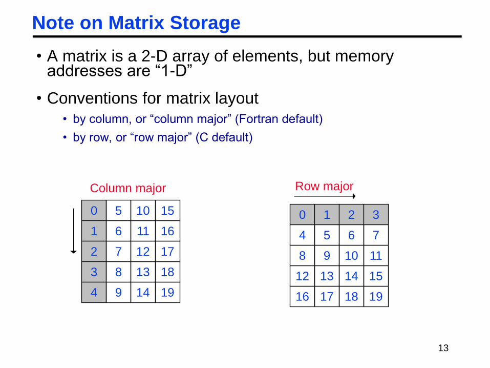
Optimizing in Practice

• Tiling for registers

• loop unrolling, use of named “register” variables

• Tiling for multiple levels of cache

• Exploiting fine-grained parallelism in processor

• superscalar; pipelining

• Complicated compiler interactions

• Automatic optimization an active research area • BeBOP: www.cs.berkeley.edu/~richie/bebop

• PHiPAC: www.icsi.berkeley.edu/~bilmes/phipac

in particular tr-98-035.ps.gz

• ATLAS: www.netlib.org/atlas

• GotoBLAS

36

PHiPAC: Portable High Performance ANSI C

Speed of n-by-n matrix multiply on Sun Ultra-1/170, peak = 330 MFlops

37

ATLAS (DGEMM n = 500)

• ATLAS is faster than all other portable BLAS implementations and it is comparable with machine-specific libraries provided by the vendor. (Incorporated in MATLAB)

0.0

100.0

200.0

300.0

400.0

500.0

600.0

700.0

800.0

900.0

AM

D Ath

lon-

600

DEC

ev5

6-53

3

DEC

ev6

-500

HP90

00/7

35/1

35

IBM

PPC

604-

112

IBM

Pow

er2-

160

IBM

Pow

er3-

200

Pentiu

m P

ro-2

00

Pentiu

m II

-266

Pentiu

m II

I-550

SGI R

1000

0ip28

-200

SGI R

1200

0ip30

-270

Sun U

ltraS

parc2

-200

Architectures

MF

LO

PS

Vendor BLAS

ATLAS BLAS

F77 BLAS

Source: Jack Dongarra

38

Summary

• Performance programming on uniprocessors requires

• understanding of fine-grained parallelism in processor

• produce good instruction mix

• understanding of memory system

• levels, costs, sizes

• improve locality

• Blocking (tiling) is a basic approach

• Techniques apply generally, but the details (e.g., block size) are architecture dependent

• Similar techniques are possible on other data structures and algorithms

39

Supplement: Strassen’s aglorithm

Conventional Block Matrix Multiply

2 by 2 block matrix multiply:

C A B A B

C A B A B

C A B A B

C A B A B

11 11 11 12 21

12 11 12 12 22

21 21 11 22 21

22 21 12 22 22

2221

1211

2221

1211

2221

1211

BB

BB

AA

AA

CC

CC

where

Strassen’s algorithm

P A A B B

P A A B

P A B B

P A B B

P A A B

P A A B B

P A A B B

1 11 22 11 22

2 21 22 11

3 11 12 22

4 22 21 11

5 11 12 22

6 21 11 11 12

7 12 22 21 22

( )( )

( )

( )

( )

( )

( )( )

( )( )

C P P P P

C P P

C P P

C P P P P

11 1 4 5 7

12 3 5

21 2 5

22 1 3 2 6

Strassen does it with 7 multiplies (but many more adds)

One matrix multiply is replaced by 14 matrix additions

Strassen’s algorithm • The count of arithmetic operations is:

• Current world’s record is O(n^2.376…)

• In reality the use of Strassen’s algorithm is limited by

• Additional memory required for storing the P matrices.

• More memory accesses are needed.

Mult Add Complexity

Regular 8 4 2n3+O(n2)

Strassen 7 18 4.7n 2.8 + O(n2)