Embed Size (px)
Citation preview

ECOSYSTEM SERVICES, HUMAN WELL-BEING, AND POLICIES IN COUPLED HUMAN AND NATURAL SYSTEMS
By
Wu Yang
A DISSERTATION
Submitted to Michigan State University
In partial fulfillment of the requirements for the degree of
Fisheries and Wildlife – Doctor of Philosophy
2013

ABSTRACT
ECOSYSTEM SERVICES, HUMAN WELL-BEING, AND POLICIES IN COUPLED HUMAN AND NATURAL SYSTEMS
By
Wu Yang
Over the past decades, human activities have led to unprecedented biodiversity losses and
socioeconomic costs. Unless effective changes in policies, institutions, and practices are made,
the deterioration is predicted to be even graver in the future. The fundamental challenge to
reverse the situation for achieving both environmental and socioeconomic sustainability lies in
improving the understanding and management of human-nature interactions.
To address such challenge, this dissertation focuses on improving the understanding of
linkages between ecosystem services (ES) and human well-being (HWB), and examining
complex policy effects on both ES and HWB. Specific objectives are to: (1) develop an
integrated approach to understand the linkages between ES and HWB; (2) understand the effects
and underlying mechanisms of indirect and direct drivers, including group size, on collective
action and ES management outcomes; (3) test the interaction effects of different policies on
HWB; (4) understand the effects of payments for ecosystem services (PES) programs on both ES
and HWB; and (5) examine the effects of the post-disaster reconstruction policy on both ES and
HWB.
To achieve my objectives, I chose Wolong Nature Reserve and the adjacent Sanjiang
Township in Sichuan Province, southwestern China as my study areas. Combining long-term
data from household surveys, field plots, and remotely sensed images as well as extensive local
knowledge, I used various methods (e.g., ordinary least-squared regression, Tobit models,

instrumental variable analysis, confirmatory factor analysis, structural equation models, and
spatial autoregressive models) to test hypotheses and answer research questions.
Major findings from this dissertation include: (1) the construction of quantitative
indicators for ES and HWB as well as integrated models is a viable approach in forwarding the
understanding of linkages between ES and HWB. Such integrated approach also generated some
important findings. For example, those who are more vulnerable to disasters are disadvantaged
households with lower access to multiple forms of capital, more property damages, or larger
revenue reductions. Diversifying human dependence on ES helps to alleviate disaster impacts on
HWB; (2) group size has nonlinear effects on both collective action and resource outcomes, with
groups of intermediate size contributing the most effort and leading to the best outcomes; (3)
there are synergistic and antagonistic effects among conservation and/or development policies,
which can even lead to unanticipated consequences; (4) the Natural Forest Conservation Program
(NFCP) had an overall positive effect on ES, and mixed effects on local livelihood. To enhance
the performance of PES programs, it is important to adapt to local conditions and integrate
mechanisms in policy design and implementation; (5) the effects of post-disaster reconstruction
efforts can differ from one scale to another. Therefore, capacity building and recovery require
integrated planning and implementation targeting each form of capital at multiple scales.
Advances in methodology and scientific knowledge from this dissertation may also be
applied to study and manage other coupled human and natural systems (CHANS). Hopefully the
accumulated knowledge from a set of literature will lead to coherent theories (e.g., human-nature
feedbacks theory, vulnerability/resilience theory of CHANS) to guide the management of
human-nature interactions.

iv
It is easy to make an argument but much more difficult to make a difference.
To those who strive to make a difference
for both nature and people.

v
ACKNOWLEDGEMENTS
Without the help and support of many people, this dissertation would not have been
completed successfully and rapidly. I would like to first thank those local people at Wolong
Nature Reserve and Sanjiang Township for their participation in our surveys across years, and
willingness to share with me their local knowledge and life experiences.
I am grateful for the support and guidance from all my committee members. I thank Dr.
Jianguo (Jack) Liu, my major advisor, for his continuous support and encouragement to
implement my ideas. I also thank him for his high expectation and for always encouraging me to
aim higher and achieve greater. I thank Dr. Thomas Dietz for his technical guidance and
insightful suggestions. I also appreciate him for sparing precious time and efforts to provide me
with constructive, meticulous, and rigorous comments and edits on our collaborative chapters. I
thank Dr. Andrés Viña for his endless advice and passion in discussing with me in all aspects as
a friend. I also thank him for his pursuit of excellence in our collaborative chapters. I thank Dr.
Daniel Boyd Kramer for his insightful suggestions in designing the human well-being instrument.
I also thank him for his timely response and constructive comments on our collaborative chapters.
I would also like to thank the logistic help and support from Wolong Administrative
Bureau and the Research Center for Eco-Environmental Sciences at Chinese Academy of
Sciences. Special acknowledgements go to Hemin Zhang, Zhiyun Ouyang, Weihua Xu, Yi Xiao,
Yan Yan, Xiaogang Shi, Meng Ming, Dong Chen, Senlong Jin, Jian Yang, Biyou Yang, Bihong
Yang, Lun Wang, Bo Wang, Maoming Wang, Jifu Wang, Datian He, Jianping Liu, Mingchong
Liu, Weihong Tan, Changyou Yang, Liang Zhang, Kaiqiang Zhang, Zhijun Zhang and Sha Zhou.
I would also thank Lin Wang for inputting part of the data.

vi
I also appreciate the inspiring discussion and emotional support from many current and
previous members in Center for Systems Integration and Sustainability, especially Neil Carter,
Xiaodong Chen, Ken Frank, Guangming He, Vanessa Hull, Shuxin Li, Yu Li, Junyan Luo,
William McConnell, Sue Nichols, William Taylor, Mao-Ning Tuanmu, and Jindong Zhang.
I would also like to thank my family and friends. I thank all my family members for their
unconditional support, apprehension, and love. I would also thank one of my best friends Qing
Zhang who shares with me both positive and negative emotions, always stands by me, trusts me,
encourages me, and feels proud of me. Any achievement that I made from the completion of this
dissertation is also theirs.
Finally, I gratefully acknowledge financial supports from the National Science
Foundation, and National Aeronautics and Space Administration of United States, and the
Environmental Science and Policy Program, College of Agriculture and Natural Resources, and
Graduate Office at Michigan State University.

vii
TABLE OF CONTENTS
LIST OF TABLES .......................................................................................................................... x
LIST OF FIGURES ..................................................................................................................... xiii
CHAPTER 1 INTRODUCTION .......................................................................................................................... 1
1.1 Background ............................................................................................................................2 1.2 Research objectives ................................................................................................................6
CHAPTER 2 GOING BEYOND THE MILLENNIUM ECOSYSTEM ASSESSMENT: AN INDEX SYSTEM OF HUMAN DEPENDENCE ON ECOSYSTEM SERVICES ..................................................... 9
Abstract .................................................................................................................................10 2.1 Introduction ..........................................................................................................................11 2.2 Methods for developing an index system of human dependence on ecosystem services ....15
2.2.1 Conceptualization of the index system ......................................................................... 15 2.2.2 Methods for constructing the index system .................................................................. 17
2.3 Empirical demonstration of constructing the index system .................................................19 2.3.1 Description of the demonstration area .......................................................................... 19 2.3.2 Data and methods ......................................................................................................... 21 2.3.3 Results of the index system .......................................................................................... 24 2.3.4 Advantages and applications of the index system ........................................................ 25
2.4 Discussion and conclusions ..................................................................................................27
CHAPTER 3 GOING BEYOND THE MILLENNIUM ECOSYSTEM ASSESSMENT: AN INDEX SYSTEM OF HUMAN WELL-BEING ........................................................................................................ 36
Abstract..................................................................................................................................37 3.1 Introduction ..........................................................................................................................38 3.2 Methods ................................................................................................................................42
3.2.1 Ethics statement ............................................................................................................ 42 3.2.2 Development of the human well-being index (HWBI) system .................................... 42 3.2.3 Description of the demonstration sites ......................................................................... 44 3.2.4 Household surveys ........................................................................................................ 46
3.3 Results ..................................................................................................................................47 3.3.1 Internal consistency of the HWBI system .................................................................... 47 3.3.2 CFA results of the HWBI system ................................................................................. 47 3.3.3 Impacts of the earthquake on HWBI ............................................................................ 48
3.4 Discussion ............................................................................................................................49 3.5 Conclusions and implications ..............................................................................................51

viii
CHAPTER 4 AN INTEGRATED APPROACH TO UNDERSTAND THE LINKAGES BETWEEN ECOSYSTEM SERVICES AND HUMAN WELL-BEING ....................................................... 58
Abstract..................................................................................................................................59 4.1 Introduction ..........................................................................................................................60 4.2 Materials and Methods .........................................................................................................64 4.3 Results ..................................................................................................................................66
4.3.1 Simultaneous impacts of the earthquake on IDES and HWBI. .................................... 66 4.3.2 Effects of IDES on change of HWBI. .......................................................................... 67 4.3.3 Effects of other indirect and direct drivers on change of HWBI. ................................. 68
4.4 Discussion ............................................................................................................................69
CHAPTER 5 NONLINEAR EFFECTS OF GROUP SIZE ON COLLECTIVE ACTION AND RESOURCE OUTCOMES................................................................................................................................. 77
Abstract..................................................................................................................................78 5.1 Introduction ..........................................................................................................................79 5.2 Materials and Methods .........................................................................................................83 5.3 Results ..................................................................................................................................85 5.4 Discussion ............................................................................................................................88
CHAPTER 6 INTERACTION EFFECTS OF CONSERVATION AND DEVELOPMENT POLICIES ON RURAL HOUSEHOLD INCOME AND INCOME STRUCTURE ............................................ 97
Abstract..................................................................................................................................98 6.1 Introduction ..........................................................................................................................99 6.2 Methods ..............................................................................................................................101
6.2.2 Data collection and analyses....................................................................................... 104 6.2.3 Econometric Models ................................................................................................... 105
6.3 Results ................................................................................................................................106 6.4 Discussion ..........................................................................................................................108
CHAPTER 7 PERFORMANCE AND PROSPECTS OF PAYMENTS FOR ECOSYSTEM SERVICES PROGRAMS: EVIDENCE FROM CHINA .............................................................................. 120
Abstract...............................................................................................................................121 7.1. Introduction .......................................................................................................................122 7.2. Materials and methods ......................................................................................................124
7.2.1. Study area .................................................................................................................. 124 7.2.2. Forest cover dynamics ............................................................................................... 127 7.2.3. Focus group, individual and household interviews ................................................... 128 7.2.4. Local adaptation and implementation of the NFCP .................................................. 129 7.2.5. Baseline for environmental benefits .......................................................................... 131
7.3. Results ...............................................................................................................................133 7.3.1. Environmental effects of the NFCP implementation ................................................ 133 7.3.2. Socioeconomic effects of NFCP implementation ..................................................... 135
7.4. Discussion .........................................................................................................................136

ix
7.4.1. Lessons learned through NFCP implementation ....................................................... 138 7.4.2. Challenges and Opportunities .................................................................................... 141
7.5. Conclusions .......................................................................................................................145
CHAPTER 8 DYNAMICS OF HOUSEHOLD CAPITAL IN PROTECTED AREAS DURING POST-DISASTER RECONSTRUCTION ............................................................................................ 154
Abstract................................................................................................................................155 8.1 Introduction ........................................................................................................................156 8.2 Materials and methods .......................................................................................................159
8.2.1 Study area ................................................................................................................... 159 8.2.2 Data collection and analyses....................................................................................... 160
8.3 Results ................................................................................................................................161 8.4 Discussion ..........................................................................................................................163
8.4.1 Causes and effects for observed changes in household capital .................................. 164 8.4.2 Policy recommendations............................................................................................. 166
8.5 Conclusion ..........................................................................................................................169
CHAPTER 9 CONCLUSIONS........................................................................................................................ 181
APPENDICES ............................................................................................................................ 186 APPENDIX A SUPPORTING INFORMATION FOR CHAPTER 2 ...................................187 APPENDIX B SUPPORTING INFORMATION FOR CHAPTER 3 ....................................189 APPENDIX C SUPPORTING INFORMATION FOR CHAPTER 4 ....................................194 APPENDIX D SUPPORTING INFORMATION FOR CHAPTER 5 ...................................198 APPENDIX E SUPPORTING INFORMATION FOR CHAPTER 6 ....................................239
REFERENCES ........................................................................................................................... 247
x
LIST OF TABLES
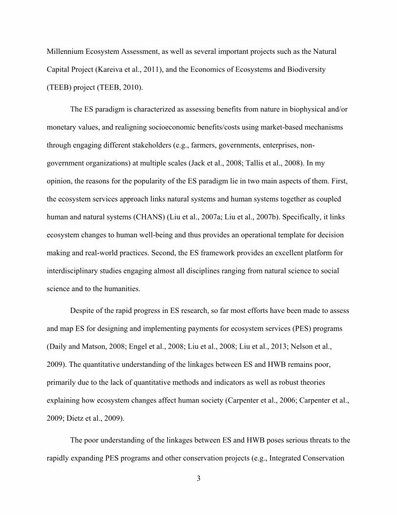
Table 2.1. Net benefits, overall IDES and sub-indices in 1998 and 2007. ................................... 32
Table 2.2. Comparison of overall IDES and agricultural income share for their associations with gross household income. ............................................................................................................... 33
Table 2.3. Regression of sources of variation on overall IDES. ................................................... 34
Table 3.1. Summary of model fit information for the confirmatory factor analysis. ................... 53
Table 3.2. Descriptive statistics of sub-indices and overall HWBI both inside and outside the reserve before and after the earthquake. ....................................................................................... 54
Table 3.3. Impacts of the earthquake on sub-indices and overall HWBI inside and outside the reserve. .......................................................................................................................................... 55
Table 4.1. Factors associated with the change of HWBI before and after the earthquake. .......... 72
Table 4.2. Example hypotheses and questions for future research on human-nature interactions........................................................................................................................................................ 73
Table 5.1. Coefficients of the Tobit model for the nonlinear effect of group size on collective action. ............................................................................................................................................ 91
Table 5.2. Coefficients of the spatial autoregressive error model for the nonlinear effect of group size on resource outcomes. ........................................................................................................... 92
Table 5.3. Path analysis of the two opposing forces through which group size affects collective action. ............................................................................................................................................ 93
Table 6.1. General information of the four conservation and development policies in Wolong Nature Reserve. ........................................................................................................................... 111
Table 6.2. Effects of conservation and development policies on changes in total household income. ........................................................................................................................................ 113
Table 6.3. Effects of conservation and development policies on changes in agricultural income percentage. .................................................................................................................................. 115
Table 7.1. General information about the PES programs in Wolong Nature Reserve. .............. 147
Table 7.2. Paired t-test for indicators of energy use before and after the NFCP implementation...................................................................................................................................................... 148
Table 8.1. The definition and selected indicators of four forms of capital. ................................ 171

xi
Table 8.2. Descriptive statistics of cropland per household inside and outside the Reserve. ..... 172
Table S2.1. Detailed classification of household net income and avoided costs by type of related ecosystem services.......................................................................................................................186
Table S3.1. The index system for assessing human well-being based on the Millennium Ecosystem Assessment conceptual framework...........................................................................188
Table S3.2. Standardized coefficients of the confirmatory factor analysis for Human Well-Being Index (HWBI)..............................................................................................................................191
Table S4.1. Descriptive statistics of variables used in the model................................................193
Table S4.2. Impacts of the earthquake on net benefits from socioeconomic activities and ecosystem services.......................................................................................................................194
Table S4.3. Associations between HWBI and affluence before and after the earthquake..........195
Table S4.4. Supplementary regressions for factors associated with the change of HWBI before and after the earthquake...............................................................................................................196
Table S5.1. Descriptive statistics of variables for 156 randomly sampled monitoring households....................................................................................................................................224
Table S5.2. Correlation between group size and other biophysical, demographic, and socioeconomic variables..............................................................................................................224
Table S5.3. Descriptive statistics of variables for 151 household-monitored parcels.................225
Table S5.4. Descriptive statistics of characteristics of 113 randomly sampled monitoring households and their assigned groups..........................................................................................225
Table S5.5. Path analysis of the two opposing forces through which group size affects collective action............................................................................................................................................226
Table S5.6. Characteristics of households with strong and weak social ties to local leaders......227
Table S5.7. Logit estimation of factors associated with social ties to local leaders....................228
Table S5.8. Tobit models for hypothesized instrumental variables.............................................229
Table S5.9. Coefficients of the Tobit model for the nonlinear effect of group size on collective action............................................................................................................................................230
Table S5.10. First-stage regression results of the two-step Tobit model.....................................231
Table S5.11. Second-stage regression results of the two-step Tobit model................................232

xii
Table S5.12. Variance inflation factors for variables used in the Tobit model examining the nonlinear group-size effect (Table 5.1 or Table S5.9).................................................................232
Table S5.13. Different combinations of Tobit models for the nonlinear effect of group size on collective action...........................................................................................................................233
Table S5.14. Coefficients of the spatial autoregressive error model for the linear effect of group size...............................................................................................................................................234
Table S5.15. Coefficients of the multiple linear regression for the nonlinear effect of group size...............................................................................................................................................235
Table S5.16. Coefficients of the spatial autoregressive error model for the nonlinear effect of group size on resource outcomes.................................................................................................236
Table S5.17. Variance inflation factors (VIFs) for variables used in the spatial simultaneous autoregressive error model (Table 5.1 or Table S5.16)...............................................................237
Table S6.1. Descriptive statistics of variables used in modeling the effects of conservation and development policies on changes in total household income and income structure...................240
Table S6.2. Complementary results of the effects of conservation and development policies on changes in total household income..............................................................................................242
Table S6.3. Complementary results of the effects of conservation and development policies on changes in the percentage of agricultural income.......................................................................244

xiii
LIST OF FIGURES
Figure 2.1. Wolong Nature Reserve in Sichuan Province, southwestern China. For interpretation of the references to color in this and all other figures, the reader is referred to the electronic version of this dissertation. ........................................................................................................... 35
Figure 3.1. Wolong Nature Reserve and adjacent Sanjiang Township in Wenchuan County, Sichuan Province, southwestern China. ........................................................................................ 56
Figure 3.2. Path diagram of the confirmatory factor analysis model for HWBI. ......................... 57
Figure 4.1. Wolong Nature Reserve in Wenchuan County, Sichuan Province, southwestern China........................................................................................................................................................ 74
Figure 4.2. Impacts of the earthquake on human dependence on ecosystem services. ................ 75
Figure 4.3. Impacts of the earthquake on human well-being. ....................................................... 76
Figure 5.1. Hypothetical effects of free riding, within-group enforcement, and group size on collective action and resource outcomes. ...................................................................................... 94
Figure 5.2. Map of the location, main road, forest cover in 2007, and household monitoring parcels of Wolong Nature Reserve in Sichuan Province, China. ................................................. 95
Figure 5.3. The nonlinear group-size effects on collective action and forest outcomes. .............. 96
Figure 6.1. Hypothetical outcomes of interaction effects among different policies. .................. 117
Figure 6.2. Wolong Nature Reserve in Sichuan Province, southwestern China. ........................ 119
Figure 7.1. Map of the Wolong Nature Reserve. ........................................................................ 149
Figure 7.2. Natural Forest Conservation Program (NFCP) implementation in the Wolong Nature Reserve (WNR). .......................................................................................................................... 150
Figure 7.3. Forest cover area before and after the Natural Forest Conservation Program (NFCP) implementation in 2001. ............................................................................................................. 151
Figure 7.4. Perceptions of local households toward the Natural Forest Conservation Program (NFCP). ....................................................................................................................................... 152
Figure 8.1. Map of Wolong Nature Reserve and the adjacent Sanjiang Township. ................... 173
Figure 8.2. Box plots of household expenditures on food (a), education (b), and medical care (c) before and after the earthquake at Wolong Nature Reserve. ...................................................... 174

xiv
Figure 8.3. Dynamics of the house type inside (a) and outside the Reserve (b) from 1970s to 2010s. .......................................................................................................................................... 176
Figure 8.4. Dynamics of the total constructed area per household (a) and loans per household for post-disaster housing repair or reconstruction (b). ..................................................................... 177
Figure 8.5. Total amount of social support and social support per lender before and after the earthquake both inside and outside the Reserve. ........................................................................ 178
Figure 8.6. Proportions of external and internal sources of social support for households before and after the earthquake both inside and outside the Reserve. ................................................... 179
Figure 8.7. Dynamics of the gross household income inside and outside the Reserve from 1970s to 2010s. ...................................................................................................................................... 180

1
CHAPTER 1
INTRODUCTION

2
1.1 Background
Over the past decades, the Earth’s ecosystems have experienced unprecedented
degradation due to human activities, which has resulted in a substantial and largely irreversible
loss of biodiversity (MA, 2005). The dramatic changes to ecosystems have substantially
contributed to human well-being (HWB) and economic development at the costs of degradation
of many ecosystem services (ES), increased risks of nonlinear changes, and the exacerbation of
poverty of some groups of people (Carpenter et al., 2006; MA, 2005). It is predicted that the
deteriorating of ecosystems could become a grave problem during the first half of this century
(MA, 2005). Unless effective changes in policies, institutions, and practices can be made, this
degradation would be a barrier to achieve sustainability identified by the United Nations
Millennium Development Goals (MA, 2005). The fundamental challenge for achieving both
environmental and socioeconomic sustainability lies in improving the understanding and
management of human-nature interactions (Carpenter et al., 2009; Liu et al., 2007a; Ostrom,
2009).
ES science has recently become a popular paradigm toward improving the understanding
and management of human-nature interactions. Studies related to this field date back to at least
the early 1980s (Fisher et al., 2009). But the paradigm began to form in late 1990s with the
publication of the influential book “Nature’s Services” (Daily, 1997) and the valuation of
world’s ES and natural capital (Costanza et al., 1997), as well as the implementation of the
payments for ES program in Costa Rica (Sanchez-Azofeifa et al., 2007). Publications using the
term “ecosystem services”, “environmental services” or “ecological services” are soaring
exponentially after the monumental Millennium Ecosystem Assessment (Fisher et al., 2009; MA,
2005). The significance of this field has gained increasing acceptance and application since the
3
Millennium Ecosystem Assessment, as well as several important projects such as the Natural
Capital Project (Kareiva et al., 2011), and the Economics of Ecosystems and Biodiversity
(TEEB) project (TEEB, 2010).
The ES paradigm is characterized as assessing benefits from nature in biophysical and/or
monetary values, and realigning socioeconomic benefits/costs using market-based mechanisms
through engaging different stakeholders (e.g., farmers, governments, enterprises, non-
government organizations) at multiple scales (Jack et al., 2008; Tallis et al., 2008). In my
opinion, the reasons for the popularity of the ES paradigm lie in two main aspects of them. First,
the ecosystem services approach links natural systems and human systems together as coupled
human and natural systems (CHANS) (Liu et al., 2007a; Liu et al., 2007b). Specifically, it links
ecosystem changes to human well-being and thus provides an operational template for decision
making and real-world practices. Second, the ES framework provides an excellent platform for
interdisciplinary studies engaging almost all disciplines ranging from natural science to social
science and to the humanities.
Despite of the rapid progress in ES research, so far most efforts have been made to assess
and map ES for designing and implementing payments for ecosystem services (PES) programs
(Daily and Matson, 2008; Engel et al., 2008; Liu et al., 2008; Liu et al., 2013; Nelson et al.,
2009). The quantitative understanding of the linkages between ES and HWB remains poor,
primarily due to the lack of quantitative methods and indicators as well as robust theories
explaining how ecosystem changes affect human society (Carpenter et al., 2006; Carpenter et al.,
2009; Dietz et al., 2009).
The poor understanding of the linkages between ES and HWB poses serious threats to the
rapidly expanding PES programs and other conservation projects (e.g., Integrated Conservation
4
and Development Projects [ICDPs]). For instance, two thirds of ICDPs implemented between
1993 and 2007 by the World Bank had failed to achieve their conservation and development dual
goals, largely due to the neglect of linkages between ES and HWB across scales (Tallis et al.,
2008). The landmark work by Ostrom and others also pointed out that the pervasive failures of
conservation policies were primarily due to ignorance of the complex linkages between ES and
HWB (Ostrom, 1990, 2005, 2007; Ostrom, 2009; Ostrom et al., 2007). The PES programs are
with no exception to such risk. First, economic values are only a subset of intrinsic values of
ecosystem and an economically driven focus on the values of ecosystems for human needs may
be detrimental to long-term survival of nonhuman components of ecosystems (Redford and
Adams, 2009). Second, ES substantially but not exclusively contribute to HWB. There are many
other factors (e.g., life experience, personality, culture, legal frameworks in which one lives)
affect the subjective feelings of humans (Diener and Ryan, 2009; Diener et al., 1999). Third,
payments to protect one service may adversely affect the provision of other services. For
example, payments for natural forest conservation may promote carbon sequestration, reduce soil
erosion and encourage wildlife proliferation, but may also increase agricultural losses to wildlife
disturbance (Liu et al., 2013). Fourthly, there is a distinction between protection of ES and
biodiversity because there are ecosystems (e.g., agricultural systems) provide important services
but are not priority biodiversity hotspots. Finally, the distribution of benefits provided by ES is
often unequal across different population groups. In comparison to the affluent, poor people may
be more dependent on the provision of ES but they usually have less control of them (Carpenter
et al., 2006; Redford and Adams, 2009). Therefore, the effectiveness of PES programs and other
conservation policies will largely depend on improving the understanding and management of
the linkages between ES and HWB.

5
While numerous conservation and development policies have been designed and
implemented to protect ES and improve HWB, relatively few studies (Arriagada et al., 2009;
Gross-Camp et al., 2012; Scullion et al., 2011) have simultaneously evaluated both the
environmental and socioeconomic outcomes. Perhaps one reason is because of the lack of
understanding and consideration of human-nature interactions discussed above. Another reason
perhaps is because of the lack of systematic collection of both environmental and socioeconomic
data before the policy implementation. Finally, it is difficult to identify a counterfactual without-
policy baseline scenario if the policy has already been implemented. Moreover, there is also a
lack of systematic and quantitative studies on underlying mechanisms of how different drivers
lead to corresponding environmental and socioeconomic outcomes. For instance, it is often
assumed that conditional cooperators (i.e., members who will contribute more for guarding
public good under the condition that others also contribute more) and costly monitoring have
positive effects to management outcomes of common-pool resources. However, until recently
this proposition and the underlying mechanisms have not been confirmed with systematically
collected data in real-world practice (Rustagi et al., 2010). The effects and underlying
mechanisms of some other factors, such as social networks and group size (i.e., the number of
group members), on collective action and common-pool resource outcomes remain elusive
(Ostrom, 2005; Tucker, 2010).
In addition, interactions among different policies are mostly ignored in previous research
(Liu et al., 2008; Liu et al., 2013). There are several good reasons to consider these interactions.
First, there are usually concurrent conservation and development policies across space and the
evaluation of each policy may be biased if there are significant interaction effects among
multiple policies (Liu and Yang, 2012; Ward and Pulido-Velazquez, 2008). Second, it will be

6
difficult to achieve different goals of multiple policies simultaneously without considering their
interactions. The above discussion on the trade-offs among different ES for PES programs is
evidence of this in reality. Third, for policies with dual goals (e.g., ICDPs) both for ES and
HWB, the linkages between ES and HWB mean that there could also be interactions among
different policy implementation strategies that separately emphasize ES or HWB. Finally,
interactions among multiple policies may generate unanticipated consequences through feedback
loops across scales. For instance, while an efficient irrigation program reduced water use on
individual farms, it increased evapotranspiration (i.e., loss of water associated with plant use),
reduced groundwater replenishment, and redistributed water supply at a water basin scale, which
actually increased overall water use at the water basin scale and beyond (Ward and Pulido-
Velazquez, 2008). A PES program that provided incentives encourage the expansion of the
efficient irrigation program also cannot reduce overall water use alone. The solution is to
combine the two policies with institutional innovations that account water use at multiple scales
aiming to reduce overall water use (Ward and Pulido-Velazquez, 2008).
1.2 Research objectives
To fill knowledge gaps discussed above, the overall goal of my dissertation is to improve
the understanding and management of human-nature interactions. Specific research objectives
include:
(1) Developing an integrated approach to understand the linkages between ecosystem services
and human well-being (Chapters 2, 3 and 4);

7
(2) Understanding the effects and underlying mechanisms of indirect and direct drivers,
especially group size (i.e., the number of group members), on collective action and ecosystem
service management outcomes (Chapter 5);
(3) Testing the interaction effects of different policies on human well-being (Chapter 6);
(4) Understanding the effects of payments for ecosystem services programs on both ecosystem
services and human well-being (Chapter 7);
(5) Examining the effects of the post-disaster reconstruction policy on both ecosystem services
and human well-being (Chapter 8).
To achieve these objectives, I chose Wolong Nature Reserve (WNR; N 30˚45' – 31˚25', E
102˚52' – 103˚24') for Giant Pandas (Ailuropoda melanoleuca) as my focus study area. Per the
needs of specific research questions in some chapters (Chapter 3 and 8), I also chose the adjacent
Sanjiang Township (SJT) as a comparison site. There are three main reasons for such selection.
The first reason is that there are long-term existing data from household surveys and field plots
dating back to 1998. There are also remotely sensed images (e.g., Landsat TM and EM) tracing
back to 1960s. The rich datasets and accumulated local knowledge lay a good foundation for
systematic experimental design and rigorous statistical analyses supporting reasonable causal
inference. The second reason is that both WNR and SJT are of high ecological importance. They
both belong to the Sichuan Giant Panda Sanctuaries of the United Nations Educational, Scientific
and Cultural Organization (UNESCO) World Heritage System. The Sanctuary was established in
2006 to protect the giant panda habitat (Li et al., 2013). It also has been classified as one of the
world’s top 25 Biodiversity Hotspots (Myers et al., 2000) and one of the Global 200 Eco-regions
identified by the World Wide Fund for Nature (WWF) (WWF, 2007). Third, both sites have

8
local residents whose ancestors settled the area hundreds of years ago. Local residents interact
with nature and depend on many ES (e.g., cultivation of maize, potatoes, yaks, pigs, cattle, and
collection of fuelwood, mushrooms, and traditional Chinese medicines) long before the
establishment of the Sanctuary. Since the late 1990s, several national and local conservation and
development policies (e.g., Natural Forest Conservation Program, Grain-to-Green Program, and
Tourism Development Plan) have been implemented in this area. On May 12, 2008, the
devastating Wenchuan Earthquake (Ms 8.0 or Mw 7.9) also hit both sites, with the epicenter
immediately near the two sites. In response to tremendous socioeconomic and environmental
impacts caused by the earthquake, a national reconstruction plan (i.e., Post-earthquake
Reconstruction Plan) has also been implemented. All these conservation and development
policies may lead to dramatic impacts on both local ES and HWB, which again provide excellent
opportunities to address my objectives.
Because all the main chapters (i.e., Chapter 2 to 8) have been published in or have been
prepared for peer-reviewed journals, more detailed background information of the study areas
including details on different conservation and development policies are provided in each of the
main chapters.

9
CHAPTER 2
GOING BEYOND THE MILLENNIUM ECOSYSTEM ASSESSMENT: AN INDEX
SYSTEM OF HUMAN DEPENDENCE ON ECOSYSTEM SERVICES
In collaboration with
Thomas Dietz, Wei Liu, Junyan Luo, Jianguo Liu
10
Abstract
The Millennium Ecosystem Assessment (MA) estimated that two thirds of ecosystem
services on the earth have degraded or are in decline due to the unprecedented scale of human
activities during recent decades. These changes will have tremendous consequences for human
well-being, and offer both risks and opportunities for a wide range of stakeholders. Yet these
risks and opportunities have not been well managed due in part to the lack of quantitative
understanding of human dependence on ecosystem services. Here, we propose an index of
dependence on ecosystem services (IDES) system to quantify human dependence on ecosystem
services. We demonstrate the construction of the IDES system using household survey data. We
show that the overall index and sub-indices can reflect the general pattern of households’
dependences on ecosystem services, and their variations across time, space, and different forms
of capital (i.e., natural, human, financial, manufactured, and social capitals). We support the
proposition that the poor are more dependent on ecosystem services and further generalize this
proposition by arguing that those disadvantaged groups who possess low levels of any form of
capital except for natural capital are more dependent on ecosystem services than those with
greater control of capital. The higher value of the overall IDES or sub-index represents the
higher dependence on the corresponding ecosystem services, and thus the higher vulnerability to
the degradation or decline of corresponding ecosystem services. The IDES system improves our
understanding of human dependence on ecosystem services. It also provides insights into
strategies for alleviating poverty, for targeting priority groups of conservation programs, and for
managing risks and opportunities due to changes of ecosystem services at multiple scales.

11
2.1 Introduction
The Millennium Ecosystem Assessment (MA) was designed to assess the consequences
of ecosystem change and provide scientific information that could aid in sustainably managing
ecosystems for human well-being (MA, 2005). Although the intended audience was decision-
makers, MA also provided a conceptual framework for studying interactions among four key
components (i.e., indirect drivers, direct drivers, ecosystem services, and human well-being) of
coupled human and natural systems (CHANS) (Liu et al., 2007a), and identified future research
needs (Carpenter et al., 2006).
Of the interactions between the four components in the MA framework, the linkage
between ecosystem services and human well-being is perhaps least understood. The relationship
between human well-being and the social factors that influence it has been extensively studied
(Abdallah et al., 2008; Campbell, 1976; Diener, 2000; Diener et al., 1999; Grant et al., 2009).
Through efforts like land change science and structural human ecology, the relationships
between changes of ecosystems services and factors that influence them have also begun to be
documented from local to regional and global scale (Rosa et al., 2010; Turner et al., 2008). It has
been recognized that humans substantially depend on ecosystem services, which range from
basic provisions of food, fresh water and fuel, through regulation of water and air quality, to
cultural services like ecotourism (Daily, 1997; MA, 2005). The MA also established that during
recent decades, two thirds of these services have degraded or are in decline due to the
unprecedented scale of human activities (MA, 2005). But what are the consequences of such
dramatic degradation to short-term and long-term human well-being? The risks of ecosystem
degradation and their consequences for human well-being, including nonlinear or abrupt changes,

12
are poorly quantified. On the one hand, there is a lack of a robust theory that links ecological
diversity to ecosystem dynamics and ecosystem services (Carpenter et al., 2006). On the other
hand, the scientific community lacks understanding of how and to what extent humans depend
on ecosystem services. For instance, it has been widely recognized that the poor are most
dependent on ecosystem services and most vulnerable to the degradation of ecosystem services
(MA, 2005); however, it is generally not known how such dependence differs across time, space
and various population groups (e.g., across income levels). To better understand, monitor and
manage such dependences, a quantitative approach is urgently needed.
From our perspective, there are at least four reasons to quantify human dependence on
ecosystem services. First, the relationship between ecosystem services and poverty seems
obvious but the dependence of the poor on ecosystem services is rarely quantified, which leads to
a pervasive tendency to overlook it in statistics, poverty assessments and natural resource
management decisions (Shackleton et al., 2008). A quantitative measurement of such
dependence and its integration into decision making could reverse inappropriate strategies that
could otherwise lead to further marginalization of the poor and increased pressure on ecosystem
services.
Second, benefits provided by ecosystem services are often unequally distributed across
different population groups and there may be trade-offs among groups. With better
understanding of the distribution of benefits from ecosystem services (e.g., fuelwood, clean
water, non-timber forest products, and tourism) across different population groups, conservation
and development programs may be better designed to guide the flow of benefits from ecosystem
services to target priority population groups. The Wolong Nature Reserve of China provides a
compelling example. Most benefits obtained from ecotourism flow to the outside tourism
13
development companies rather than local households (He et al., 2008; Liu et al., 2012), a
common phenomenon in many other areas (Kiss, 2004). Government policies should encourage
household relocation closer to tourism facilities and provide more support to local households
(e.g., provide training to improve human capital and offer favorable loan opportunities) to
enhance their capacity for participating in tourism businesses (He et al., 2008; Liu et al., 2012).
In doing so, more benefits from tourism would flow to local households and substantially reduce
their pressure on provisioning services by which local ecosystems provide fuelwood, bamboo
shoots, and traditional Chinese medicine.
Third, a better understanding of such dependence would draw attention to currently
unmanaged risks and unrealized opportunities that come with ecosystem change. For example,
agricultural supply chains can be tightly dependent on ecosystem services and thus are
vulnerable to dramatic ecosystem degradation. Unprecedented human activities would likely lead
to more frequent extreme climate events and natural disasters (e.g., storms, floods, droughts, and
landslides), cause tremendous destruction to ecosystems and their services, and threaten the
livelihoods of those people who are highly dependent on corresponding ecosystem services (MA,
2005; Rosa et al., 2010). Yet few managers or policy analysts understand this dependence and
related unintended consequences, and even fewer manage the potential risks and opportunities
(Grigg, 2008; Liu and Yang, 2012).
Fourthly, a quantitative measurement of such dependence would improve the
understanding of human-nature interactions. One of the major advances and challenges of the
CHANS approach for studying human-nature interactions is to construct coupled models by
integrating sub-models of both human and natural subsystems (McConnell et al., 2011). The key
of such integration requires good understanding of the interactions between human and natural

14
subsystems. Currently, there are few coupled models integrating drivers, ecosystem services, and
human well-being to systematically understand human-nature interactions (Carpenter et al., 2006;
Carpenter et al., 2009; Yang et al., 2013a). The quantification of human dependence on
ecosystem services could potentially serve as a proxy to facilitate such integration and
understanding.
The objectives of this study were to (1) propose the conceptual basis of an index of
dependence on ecosystem services (IDES) system to measure the degree of human dependence
on ecosystem services; (2) demonstrate the construction of the IDES system with empirical data;
and (3) illustrate advantages and applications of the proposed IDES system. Specifically, we first
provided the conceptual basis of an IDES system, including an overall index and sub-indices for
different categories of ecosystem services based on the widely accepted MA framework. We
then delineated the process of estimating the indices at Wolong Nature Reserve. We examined
temporal changes of the overall IDES and shifts in of the structure of the IDES system (i.e.,
changes of sub-indices). We compared the overall index with an alternative indicator (i.e., the
commonly used agricultural income share) to illustrate the advantages of our proposed index
system. Moreover, we assessed the dependence of the poor on ecosystem services. In particular,
we analyzed how households’ dependences on ecosystem services differ across different degrees
of access to capitals (i.e., natural, human, financial, manufactured, and social capitals). We also
evaluated the spatial heterogeneity of the overall IDES.

15
2.2 Methods for developing an index system of human dependence on ecosystem services
2.2.1 Conceptualization of the index system
The term ecosystem services is defined and used in a variety of ways (Boyd and Banzhaf,
2007; Costanza et al., 1997; Daily, 1997; Farber et al., 2002; MA, 2005; Wallace, 2008; Wallace,
2007). Here we aligned with the definitions of the MA as the benefits that people obtain directly
or indirectly from ecosystems, including both natural systems or highly managed systems (MA,
2005). In particular, we included agricultural products as part of ecosystem services. We
acknowledge that some literatures might exclude products from highly managed systems (e.g.,
agro-ecosystems and constructed wetlands) and restrict ecosystem services to goods and services
provided by natural systems only. But since the logic of our analysis is driven by the MA, we felt
it appropriate to adhere to the definition by the MA. Our proposed index system of dependence
on ecosystem services includes an overall index and three sub-indices. The overall index of
human dependence on ecosystem services is defined as the ratio of net benefits obtained from
ecosystems to the absolute value of total net benefits that derived from ecosystems and other
socioeconomic activities (e.g., migrant work, and small business unrelated to ecosystem services,
see Table S2.1). In addition to the overall index, a sub-index can be calculated for each category
of ecosystem services under the MA framework (i.e., provisioning, regulating services, and
cultural services) (MA, 2005). Because supporting services are the bases for other three types of
services, following the common practice in ecosystem service assessment, they are not included
in IDES to avoid double accounting. As shown by the definition, the higher value of the overall
index or sub-index represents the higher dependence on the corresponding ecosystem services,
and thus the higher vulnerability to the degradation or decline of corresponding ecosystem
services. The equations for calculating three sub-indices and the overall IDES are given as below.

16
||/3
1 i iii SNBENBENBIDES (2.1)
31i iIDESIDES (2.2)
where i is the category of ecosystem services (i.e., provisioning, regulating, and cultural services);
IDESi is the sub-index for category i; ENBi is the total net benefit obtained from category i
ecosystem services; SNB is the total net benefit obtained from socioeconomic activities; IDES is
the overall index.
There are four reasons for using net benefits instead of gross benefits. First, ecosystems
generate both services and dis-services to humans. Dis-services may include pests and diseases
causing reduction in agricultural production and other unintended negative health consequences
for organisms including humans (Zhang et al., 2007). Second, the generation and delivery of
ecosystem services may entail costs (e.g., costs of seeds, fertilizers, and pesticides for
agricultural products). Using the gross benefits could potentially mislead decision making
(Naidoo and Ricketts, 2006). One might opt for a program that has the largest increase in gross
benefits when another program has a larger yield of net benefits, thereby choosing an inefficient
program. Third, using net benefits allows the inclusion of trade-offs between different ecosystem
services (Nelson et al., 2009). Such trade-offs would not be correctly represented if gross
benefits are used without considering the costs of delivering those services. Finally, using net
benefits facilitates cross-context comparisons. Few previous ecosystem service assessments have
evaluated net benefits (Birch et al., 2010; Chang et al., 2011; Yang et al., 2008). Many previous
studies have evaluated only the gross benefits so results from different studies are not

17
comparable because ecosystem dis-services and costs of generating ecosystem services can be
substantial and vary considerably across contexts.
Both the sub-indices and overall index can be negative. This is because net benefits are
not necessarily positive. Total net benefits from each category and all categories of ecosystem
services summed can be negative. The ecological and economic meaning of an index with
negative value is that the gross benefit obtained from ecosystem services is lower than the sum of
costs for generating the corresponding ecosystem services and costs of ecosystem dis-services.
For example, the gross benefits of producing agricultural products may be lower than the total
costs of seeds, fertilizers, and pesticides.
2.2.2 Methods for constructing the index system
The index system is constructed to assess net benefits of a unit of analysis (e.g.,
household). The procedures for this approach are in some ways similar to that of many Cost-
Benefit Analyses (CBA) (Boardman et al., 2006; Hanley et al., 2001) and Ecosystem Service
Assessments (ESA) (Chang et al., 2011; MA, 2005; Nelson et al., 2009; Yang et al., 2008) where
data from a variety of sources are aggregated into an integrated assessment and where the unit of
analysis for which the calculation is done must be specified. For CBA and ESA this is often a
region or nation, while here we will work at the household level.
Where markets for the gross benefits and costs exist, assessments are relatively
straightforward and simple. It is easy to apply market-based valuation methods such as the
market price method, the appraisal method, and the avoided cost method (Barbier, 2011; Chee,
2004; Scott et al., 1998; Yang et al., 2008). Otherwise, when market data are not available,
18
nonmarket valuation methods such as the contingent valuation method, the travel cost method,
the stated preference method, and the hedonic price method can be used (Barbier, 2011; Bateman
et al., 2011; Scott et al., 1998; Yang et al., 2008).There are also cross-cutting methods, such as
the benefit transfer method and unit-day value method, which combine both market-based and
nonmarket methods (Ready and Navrud, 2006; Shrestha et al., 2007; Wilson and Hoehn, 2006).
Recently, integrated approaches such as the Integrated Valuation for Ecosystem Services and
Tradeoffs (InVEST) have focused on assessing ecological production and then applying
economic valuation methods (Kareiva et al., 2011; Nelson et al., 2009). A variety of reviews and
guidelines have discussed these economic valuation methods in detail (e.g., (Barbier, 2011;
Boardman et al., 2006; Hanley et al., 2001; Richard et al., 2001)). A summary and critique of the
use of these methods was presented by Bateman (Bateman et al., 2011) and thus we do not
discuss the use of these economic valuation methods in detail here. We provided an example of
how different types of data could be collected through various economic valuation methods to
assess the net benefits for constructing the IDES system. The following empirical study will
demonstrate the integration of different data sources and valuation methods in detail.
Consider a rural household living in a forest area as an example. Costs and benefits from
agricultural products and other socioeconomic activities are parts of the household’s income and
expenditures and could be captured in a survey with relative ease, using best practices for
economic surveys. But when benefits or avoided costs that do not involve market transaction
(e.g., non-timber forest products such as fruits, herbal medicine, and fuelwood), they are not
shown in the household’s income and expenditures as conventionally defined and thus are not
captured by conventional economic survey methods. If there are established payments for
ecosystem services (PES) programs, then the obtained benefits (e.g., payments) and associated

19
costs (e.g., labor costs for monitoring forests) have market values. If such PES programs are not
in place, an ESA can be conducted by adding corresponding survey questions, for example by
using contingent valuation method (see case studies in (Hanley et al., 1998; Yang et al., 2008)).
An ESA can also be conducted using integrated tools such as InVEST for the entire study area
(see case studies in (Kareiva et al., 2011; Nelson et al., 2009)) and then disaggregating to the
household level (e.g., divided by total number of households in the entire study area or calculated
by defining a buffer zone of accessibility to certain ecosystem services based on each
household’s location, see an example of fuelwood collection in (He et al., 2009)).
2.3 Empirical demonstration of constructing the index system
2.3.1 Description of the demonstration area
Here we provide an example to demonstrate the index system at Wolong Nature Reserve
(N 30˚45’ - 31˚25’, E 102˚52’ - 103˚24’, Fig. 2.1) in China. We choose Wolong Nature Reserve
as our study area for three reasons. First, situated in the transition from Sichuan Basin to the
Qinghai-Tibet Plateau, it is within one of the top 25 global biodiversity hotspots endowed with
enormous ecosystem services (Liu et al., 2003a; Myers et al., 2000). Second, it is one of the
earliest nature reserves established in China (Liu et al., 2001). Like many other protected areas,
there are human residents living inside who depend on many types of ecosystem services. Third,
our research team has been conducting studies in this area over the past 18 years and has
accumulated extensive datasets and local knowledge that give us a well-grounded basis for
testing the IDES concept, methods and applications.

20
The primary purpose of Wolong Nature Reserve is to protect giant pandas (Ailuropoda
melanoleuca) as well as regional forest ecosystems and rare plant and animal species (Wolong
Nature Reserve, 2005). When it was established in 1963, its initial size was ~20,000 ha but was
expanded to its current size of ~200,000 ha in 1975 (Wolong Nature Reserve, 2005). It is home
to ~10% of the total wild giant panda population (Wolong Nature Reserve, 2005). Currently,
there are ~4,900 local human residents, distributed in ~1,200 households in two townships (i.e.,
Wolong and Gengda Townships) within the Reserve (Fig. 2.1). The majority of local residents
are farmers involved in subsistence activities such as cultivating maize and vegetables, raising
livestock (e.g., pigs, cattle, yaks, and horses), collecting traditional Chinese medicine, keeping
bees, and collecting fuelwood for cooking and heating (Table S2.1).
In response to the massive droughts in 1997 and floods in 1998, the Chinese government
started to implement a series of ecosystem service policies (Liu et al., 2008; Liu et al., 2013),
including two of the world’s largest payments for ecosystem services (PES) programs: the
Natural Forest Conservation Program (NFCP) and the Grain-to-Green Program (GTGP) (Liu et
al., 2008). These PES programs aim mainly to improve regulating services such as soil erosion
control, water conservation, carbon sequestration, and air purification. From 2000, Wolong
Nature Reserve started to implement GTGP, NFCP, as well as a local PES program called the
Grain-to-Bamboo Program (GTBP) (Wolong Nature Reserve, 2005; Yang et al., 2013e). NFCP
aims to conserve and restore natural forests through logging bans, afforestation, and monitoring,
using PES approach to motivate conservation behavior (Liu et al., 2008; Yang et al., 2013e).
GTGP and GTBP aim to convert cropland on steep slopes to forest/grassland, and bamboo forest
by providing farmers with subsidies, respectively (Liu et al., 2008; Wolong Nature Reserve,
2005; Yang et al., 2013e).

21
2.3.2 Data and methods
The household survey data used here were collected with the permission from the
Wolong Administration Bureau of Wolong Nature Reserve. A verbal consent process from
interviewees was used due to the low level of education of our interviewees. The verbal consent
script was read to the selected interviewees before conducting the survey. Only when they agreed
to participate in our survey, we then continued to ask questions in the designed survey
instruments. Or else, we did not collect any information but switched to the next selected
interviewee. The Institutional Review Board of Michigan State University
(http://www.humanresearch.msu.edu/) approved the verbal consent process, verbal consent script,
and survey instruments.
For this study we used household survey data to estimate the obtained net benefits from
ecosystem services (or equivalently gross benefits and costs) for households. This allows us to
construct the IDES estimates for households. Our surveys were conducted in the summer of 1999
and the end of 2007 to obtain data covering activities in 1998 and 2007. We tracked the same
randomly sampled 180 households so the data constitutes a panel. Usually the household heads
or their spouses were chosen as interviewees because our past experience indicates that they are
the decision makers and are most familiar with household affairs (An et al., 2001). To facilitate
cross-context comparisons, we used the categories for household income and expenditure data
that are consistent with those of the National Bureau of Statistics of China (National Bureau of
Statistics of China, 2011) and thus with standard economic survey methods. We used the MA
classification for ecosystem services to generate sub-indices. It is important to note that it is
impractical, if not impossible, to assess all the ecosystem services in a study area. This analysis

22
only attempts to include as many major ecosystem services as possible using the best available
data in our study area.
As the term implies direct ecosystem benefits are those that are used directly in
generating human well-being. For example, agricultural products are provisioning services that
provide direct benefits from agricultural ecosystems. Other services contribute indirectly to
human well-being. Sometimes indirect benefits are only one step removed from direct benefits
(i.e., first-order indirect benefits) and sometimes they are more distantly linked (i.e., secondary
or more distant indirect benefits). For example, local households do not directly partake in the
ecotourism activities but they one-step indirectly benefit from the cultural services of ecotourism
through providing transportation, food and accommodation services to eco-tourists. But
ecotourism may also enhance the development of infrastructure (e.g., road construction), create
more job opportunities, and thus provide indirect benefits several steps removed from the
cultural services. Generally, the challenge in identifying benefits for CBA is to separate the
genuine indirect effects from those that are double accounting (De Rus, 2010). Usually, if there
is not a strong rationale, only direct benefits and costs are included to avoid double accounting
(Boardman et al., 2006). However, in our study area, first-order indirect benefits capture an
important part of benefits from ecosystem services and the inclusion of them do not cause
double-accounting (Table S2.1). As a first approximation, here we included direct benefits and
first-order indirect benefits in our calculations because these captured the majority benefits in our
study area (Table S2.1). We adapted the MA classification for types of related ecosystem
services (Table S2.1) to make it appropriate for our study area. For some specific services, the
classification may differ from what would be appropriate in other areas. But this does not affect

23
the comparisons using the overall index and sub-indices of IDES, which are based on the
generalizable MA framework.
Some households obtained negative net benefits in agricultural operating income when
the total gross agricultural income was lower than total agricultural expenditure, due to pests,
diseases, natural disasters (e.g., storms and landslides), and/or low prices of agricultural products.
Most income from ecosystem services comes from provisioning services, but some households
also have income from ecotourism, which we categorized as benefits related to cultural services,
and income from PES programs, which we categorized as benefits related to regulating services
(Table S2.1).
The benefits that households obtained from ecosystems include not only the benefits
reflected in their income, but also the avoided costs not reflected in their expenditures. Two
major items of avoided costs were assessed here. One is the reduced electricity fees through a
subsidized electricity price. Because the conservation of forests also dramatically conserves
watersheds in our study area, local households were given a reduction of electricity price of 0.07
yuan per kilowatt-hour in both 1998 and 2007 (yuan: Chinese Currency, 1 USD = 7.52 yuan as
of 2007). Thus, the avoided electricity fees could be calculated by multiplying their consumed
electricity amount and the reduced price. Another item of avoided cost is from fuelwood
collection for energy use. Households would need to pay for alternative energy sources (e.g.,
electricity, coal) if they do not collect fuelwood. Because households need to spend labor
collecting fuelwood, in the past when one household did not have enough laborers in the
fuelwood collection season, one might exchange laborers or hire laborers from other households.
Thus, the monetary value of collected fuelwood can be estimated as the market value of the labor
spent on collecting it. In our household survey, we measured the collected amount of fuelwood

24
and total labor spent in collecting it. We then calculated the shadow price of fuelwood
(approximately 0.10 yuan per kilogram in 1998 and 0.20 yuan per kilogram in 2007). Data for
each household on each of these sources of net income and avoided costs were then used to
construct the index system.
2.3.3 Results of the index system
Table 2.1 showed the results of net benefits from different sources and the overall IDES
and corresponding sub-indices in both 1998 and 2007. Our results showed a dramatic increase of
net benefits from all categories of ecosystem services and socioeconomic activities. From 1998
to 2007, the total net benefit from ecosystem services has increased from an average of
approximately 1,723 yuan to 12,972 yuan (both values were in present values for 1998).
Meanwhile, from 1998 to 2007, the total net benefit from socioeconomic activities also has
dramatically increased from an average of approximately 2,456 yuan to 12,350 yuan.
Table 2.1 also showed that the overall index of households’ dependences on ecosystem
services has increased from approximately 0.42 in 1998 to 0.61 in 2007. The average overall
IDESs were 0.45 in 1998 and 0.61 in 2007, indicating that approximately 45% and 61% of total
net benefits to households came from ecosystem services in 1998 and 2007, respectively.
Approximately 54% and 63% households had an overall IDES larger than 0.50, and 9% and 16%
households had an overall IDES of 1.00 in 1998 and 2007, respectively. Overall these results
suggested that most households in our study area were highly dependent on ecosystem services
and some were essentially completely dependent on them.

25
The percent of households obtained positive net benefits from provisioning services were
89% and 85% in 1998 and 2007, respectively. Almost all households benefited from regulating
services in both 1998 and 2007. Perhaps most interesting, almost all households in 2007 acquired
positive net benefits from regulating services through the PES programs (i.e., NFCP, GTGP, and
GTBP). These programs were the major reason for the dramatic increase of net benefits from
regulating services. However, almost no household in 1998 and only 11% households obtained
positive net benefits from cultural services such as ecotourism.
2.3.4 Advantages and applications of the index system
Our IDES is better than the agricultural income share in reflecting households’
dependences on ecosystem services. Agricultural income share, or the ratio of agricultural
income to total income, is a commonly used indicator that can approximately reflect a rural
household’s dependence on ecosystem services. Although the proposition that the poor are more
dependent on ecosystem services is rarely examined quantitatively, it is a widely accepted notion
(Carpenter et al., 2006; Shackleton et al., 2008). Here, we compared the overall IDES with
agricultural income share by examining their relation to overall household income. Our results
suggested that the overall IDES were negatively associated with household income in both 1998
and 2007 (Table 2.2).That is, higher income households make less use of ecosystem services.
These results confirmed the common view that low incomes households are more dependent on
ecosystem services. However, the association of household income with agricultural income
share was significant only in 1998 but not in 2007 (Table 2.2). These results indicated that our
overall IDES was better than the agricultural income share as a measure of rural households’

26
dependences on ecosystem services. In our study area, income had become decoupled from
income share from agriculture but not from use of ecosystem services by our second survey.
Comparing the results of the index system in 1998 and 2007 (Table 2.1), the reasons that
IDES is a better measure than agricultural income share are easy to see. In 1998, most of the
household income was from agriculture, which was classified as benefits related to provisioning
services (Table S2.1). The overall IDES was almost equivalent to the sub-index for provisioning
services (Table 2.1) and thus was similar to agricultural income share in reflecting a household’s
dependence on ecosystem services in 1998. In 2007, household income sources became more
diverse and included many non-agricultural items (Table S2.1). Therefore, unlike the overall
IDES, agricultural income share no longer accurately reflected households’ dependences on
ecosystem services.
These results demonstrate some of the uses of the index system. We further illustrated its
applications by examining how the benefits of ecosystem services were unequally available to
households. Because ecosystem services flow from natural capital, households who possess
substantial access to natural capital should obtain more benefits from ecosystems and thus would
be more dependent on ecosystem services than those with less access to natural capital. The
positive associations between indices of dependence on ecosystem services and the area of
cropland supported this argument (Table 2.3). Although poverty is often defined in terms of low
access to financial capital, households in financial poverty often have limited access to human,
manufactured, and social capital. Thus, the proposition that the poor depend more on ecosystem
services may be generalized from poverty in financial capital to poverty in human, manufactured,
and social capital. Table 2.3 supported such negative associations between indices of high

27
dependence on ecosystem services and a number of measures of low access to different forms of
capital.
It should be noted that the relationship between dependence on ecosystem services and
lack of access to forms of capital can change rather rapidly. In 1998, the local economy at
Wolong Nature Reserve was relatively closed and mainly relied on agriculture. Since 2000, the
NFCP, GTGP, GTBP, and tourism development have led to more non-farm income. The local
economy became more open. For example, thousands of tourists visit Wolong Nature Reserve
every year to view giant pandas. As a result, local farmers began to grow vegetables selling to
outside markets, and some young farmers enrolled their cropland in GTGP and GTBP and
migrated to urban areas for work. These were the reasons why some indicators of capital such as
the distance to the main road, area of cropland, social ties were not as important in 1998 as they
were in 2007 (Table 2.3). Furthermore, most households in 1998 lived in low quality wooden or
stone sheds, while in 2007, with more money available, some of them lived in high quality
concrete houses. Households actively strategize how to substitute one form of capital for another
in order to achieve access to needed resources and enhance well-being (Chen et al., 2012a).
2.4 Discussion and conclusions
This proposed index system is a step forward in quantifying human dependence on
ecosystem services. As mentioned above, it is impractical, if not impossible, to capture all
ecosystem services in any study. However, we have implemented the index system with existing
household survey data and were able to capture major ecosystem services in our initial estimates.
Our results suggest that such an approximation is a viable approach that reveals useful

28
information on human dependence on ecosystem services. The overall index and its sub-indices
can reveal the general pattern of households’ dependences on ecosystem services, and the
variations across time, space, and different levels of access to multiple forms of capital.
Given the fact that different individuals, households and communities rely on different
ecosystem services, in practice it is likely that the measurement of benefits, costs and IDES will
depend on relatively detailed data that is collected with an understanding of the local context. To
facilitate comparisons across time, space and different institutional levels, it is necessary that
different studies use a common platform such as the generally accepted MA framework for
classification. While it will usually not be possible to capture all benefits and costs associated
with ecosystems services, care should be taken to accurately estimate the most important benefits
and costs in the local context in order to construct overall IDES estimates. To avoid
misinterpretation in some circumstances (e.g., the effect of Integrated Conservation and
Development Projects on changes in households’ dependence on ecosystem services), such
comparisons should not only focus on the overall IDES index but also consider the sub-indices
as well as the structure of dependence on ecosystem services (i.e., the distribution of three sub-
indices).
It should be noted that IDES measures the relative importance of ecosystem services,
with comparison to other socioeconomic activities, in providing benefits directly and indirectly
to humans. If one wants to compare the absolute values of benefits from ecosystem services
across different areas, one should use the net benefits obtained from ecosystem services, which
are also provided through construction of the IDES system.
29
It should also be noted that there is a substantial difference between being dependent on
ecosystem services and being dependent on PES. The PES program compensates some of the
forgone benefits that local households enjoyed before the implementation of conservation
policies. But the PES program does not necessarily compensate all the forgone benefits. For
example, in our study area, the main purpose of payments from NFCP is to protect natural forests.
As a result payments from NFCP mostly compensate the forgone provisioning (e.g., timber
harvest) services whereby regulating services (e.g., soil erosion control, carbon sequestration,
and water conservation) are increased. Cultural services (e.g., recreation and ecotourism) are not
included. In our study, we therefore included benefits from ecotourism which are not captured in
the PES from the NFCP.
Using the overall IDES, we confirmed the proposition that the poor are more dependent
on ecosystem services, and thus are more vulnerable to degradation or decline of the
corresponding ecosystem services. More importantly, we generalized this proposition to those
disadvantaged groups who possess less access to multiple forms of capital (i.e., human, financial,
manufactured, and social capital) and found they too were more dependent on ecosystem
services than the affluent.
Although we demonstrated the construction of the IDES system and its applications
based only on data from the Wolong Nature Reserve, the conceptual basis of IDES and
methodology we used were designed to be generalizable. While we examined households, the
unit of analysis could range from individuals to communities, regions, and nations. Our analysis
here is a proof of the concept of IDES. Further elaborations are warranted and could potentially
improve the estimates of human dependence on ecosystem services.

30
We believe the IDES index system presented here has some major advantages to advance
the understandings of linkages between ecosystem services and human well-being and support
decision-making. First, this paper empirically demonstrated how the index system could better
reflect human dependence on ecosystem services than the other commonly used indicator (i.e.,
agricultural income share) at the household level. Second, the index system provides both a
composite index and sub-indices. This allows the quantitative analysis of the structure of human
dependence on ecosystem services and the quantitative examination of the interwoven linkages
between different types of ecosystem services and different components of human well-being.
Future studies could combine IDES with indicators of indirect drivers, direct drivers, and human
well-being to construct integrated models based on the MA framework to better understand
complex interactions among human and natural components (e.g., to assess how human
dependence on ecosystem services may affect human well-being). The improved understanding
may help to develop theories on the complexity of CHANS and inform decision making in a
rapidly changing global environment. Third, the improved understanding of linkages between
ecosystem services and human well-being, if integrated into decision-making, may avoid some
inappropriate strategies that aggravate the marginalization of disadvantaged groups. This in turn
could reduce the pressure these groups place on ecosystems to obtain services critical to them.
However, a distinction should be made: dependence on ecosystem services is not equivalent to
pressure on ecosystems because there are often sustainable ways to extract ecosystem services.
Acquisitions of regulating and cultural services (e.g., air purification and ecotourism) are often
non-consumptive, while many uses of provisioning services (e.g., timber, fuelwood) are often
consumptive and may or may not be sustainable. The reduction of pressure or impacts on
ecosystem services can be realized through reduction of overall dependence on ecosystem

31
services or through a shift of the structure of dependence to different types of ecosystem services
such as a shift from high dependence on provisioning services to high dependence on regulating
and cultural services. It can also be achieved by extracting provisioning services in ways that do
not harm the ecosystem. Fourthly, improved understanding may also enhance the effectiveness
and long-term viability of conservation and development programs by targeting priority
population groups such as those with limited access to capital and high dependence on
provisioning services. Finally, such understanding could draw stakeholders’ attention to the
unmanaged risks and unrealized opportunities associated with ecosystem service changes.
Climate change and other global changes are causing rapid shifts in ecosystem structure and
function and may threaten continued flow of services to those most dependent upon them.
Taking our study area as an example, conservation and development efforts such as NFCP,
GTGP, GTBP, and tourism development have already reduced many households’ dependences
on provisioning services; however, the very uneven distribution of benefits from ecosystem
services may create potential risks and impede the future success of such policies.

32
Table 2.1. Net benefits, overall IDES and sub-indices in 1998 and 2007.
Net benefits/Indices
1998 2007 Mean (S.D.) Range
(Minimum:
Maximum) *
Mean (S.D.) Range (Minimum : Maximum)
Net socioeconomic benefit (yuan)
2456.38 (3315.50)
(0 : 16,600) 12,350.10 (21,027.75)
(0 : 186,046)
Net benefit from provisioning services (yuan)
2308.77 (2506.89)
(– 2671 : 13,676)
8544.97 (14,063.43)
(– 2620 : 107,003)
Net benefit from regulating services (yuan)
77.60 (92.88) (0 : 544) 2900.64 (2003.59)
(0 : 10,448)
Net benefit from cultural services (yuan)
3.33 (44.72) (0 : 600) 1526.10 (13,476.34)
(0 : 177,626)
Total net benefit from ecosystem services (yuan)
2389.71 (2527.22)
(– 2620 : 14,182)
12971.70 (19,043.19)
(– 27 : 181,801)
Sub-index for provisioning services
0.4131 (0.8627)
(– 7.0351 : 0.9973)
0.3754 (0.3131)
(– 0.1750 : 1)
Sub-index for regulating services
0.0340 (0.0714)
(0 : 0.7518) 0.2112 (0.2026)
(0 : 1)
Sub-index for cultural services
0.0003 (0.0038)
(0 : 0.0513) 0.0257 (0.1143)
(0 : 0.8568)
Overall IDES 0.4473 (0.8237)
(– 6.9019 : 1) 0.6123 (0.3055)
(– 0.0015 : 1)
Notes: Monetary values for net benefits in 2007 were discounted into present values of 1998 for
comparison. * Negative value of an index means that the gross benefit from ecosystem services
is lower than the sum of costs from ecosystem dis-services and costs of generating the corresponding ecosystem services.

33
Table 2.2. Comparison of overall IDES and agricultural income share for their associations with gross household income. Household income in 1998 Household income in 2007
Agricultural income share – 0.355*** – 0.012
Overall IDES – 0.194**
– 0.405***
Notes: Numbers are Spearman’s rhos. Total samples are the same 180 randomly sampled
households across years. *p < 0.05;
**p < 0.01;
***p < 0.001.

34
Table 2.3. Regression of sources of variation on overall IDES. Variable IDES 1998 IDES 2007
Natural capital Area of cropland (Mu, 1 Mu = 1/15 ha)
0.020 (0.014) 0.042***
(0.007)
Human capital Household size – 0.077 (0.049) – 0.037* (0.016)
Number of laborers – 0.070 (0.056) – 0.080***
(0.018)
Average education of adults (year) – 0.032
† (0.017) – 0.032
*** (0.009)
Average age of adults (year) 0.011* (0.005) 0.008
*** (0.002)
Financial capital Household income (yuan, log)
0.071 (0.075) – 0.152***
(0.025)
Per capital income (yuan, log)
0.143 (0.095) – 0.126***
(0.028)
Manufactured capital
Type of house (0 for low quality non-concrete sheds and 1 for high quality concrete house)
– 0.022 (0.139) – 0.189***
(0.048)
Distance to the main road (meter, log)
– 0.029 (0.027) 0.042***
(0.010)
Social capital Social ties to local township and reserve level officials (0: low; 1: high).
0.065 (0.129) – 0.188** (0.065)
Spatial heterogeneity
Township (0: Gengda; 1: Wolong)
0.098 (0.133) – 0.101* (0.047)
Notes: Numbers outside and inside parentheses are coefficients and robust standard errors of bivariate regressions, respectively. Dependent variables are overall IDES in 1998 and 2007,
respectively. Total samples are the same 180 randomly sampled households across years. †p<
0.01; *p < 0.05;
**p < 0.01;
***p < 0.001.

35
Figure 2.1. Wolong Nature Reserve in Sichuan Province, southwestern China. For interpretation of the references to color in this and all other figures, the reader is referred to the electronic version of this dissertation.

36
CHAPTER 3
GOING BEYOND THE MILLENNIUM ECOSYSTEM ASSESSMENT: AN INDEX
SYSTEM OF HUMAN WELL-BEING
In collaboration with
Thomas Dietz, Daniel Boyd Kramer, Xiaodong Chen, Jianguo Liu

37
Abstract
Understanding the linkages between ecosystem services (ES) and human well-being
(HWB) is crucial to sustain the flow of ES for HWB. The Millennium Ecosystem Assessment
(MA) provided a state-of-the-art synthesis of such knowledge. However, due to the complexity
of the linkages between ES and HWB, there are still many knowledge gaps, and in particular a
lack of quantitative indicators and integrated models based on the MA framework. To fill some
of these research needs, we developed a quantitative index system to measure HWB, and
assessed the impacts of an external driver— the 2008 Wenchuan Earthquake— on HWB. Our
results suggest that our proposed index system of HWB is well-designed, valid and could be
useful for better understanding the linkages between ES and HWB. The earthquake significantly
affected households’ well-being in our demonstration sites. Such impacts differed across space
and across the five dimensions of the sub-index (i.e., the basic material for good life, security,
health, good social relations, and freedom of choice and action). Since the conceptual framework
is based on the generalizable MA framework, our methods should also be applicable to other
study areas.

38
3.1 Introduction
Understanding the linkages between ecosystem services (ES) and human well-being
(HWB) is crucial to sustain the flow of ES for HWB (MA, 2005). The Millennium Ecosystem
Assessment (MA) was intended to provide a state-of-the-art synthesis of such knowledge. ES are
defined as the benefits human directly and indirectly obtained from ecosystems (Daily, 1997;
MA, 2005). The MA suggested that ecosystems provide services that are of importance for
improvements of HWB at multiple scales. These services range from provisioning services such
as clean water, food, and forest products, through regulating services such as flood control, soil
retention, and air purification, to cultural services such as ecotourism, aesthetic appreciation, and
a sense of place (MA, 2005). However, during the past five decades, such improvements of
HWB were achieved at escalating costs due to the decline or degradation of more than 60% of
ES across the globe. This decline or degradation in ES may increase the risks of nonlinear or
abrupt changes, and may lead to further marginalization of some groups of people (MA, 2005).
Although the MA is a monumental work, the linkages between ES and HWB are
complex and remain poorly understood (Butler and Oluoch-Kosura, 2006; Carpenter et al., 2006;
Carpenter et al., 2009). There are four major challenges in developing better understanding of
such linkages. First, HWB itself is an evolving and complex concept (Butler and Oluoch-Kosura,
2006). It is difficult to provide a universally acceptable definition of HWB. In the MA, HWB has
five constituents: the basic material for a good life, security, health, good social relations, and
freedom of choice and action (MA, 2005). Second, ES substantially, but not exclusively,
contribute to HWB. We interpret MA’s definition of HWB as the satisfaction of human needs
(Maslow, 1943) to achieve a state of being well (i.e., healthy, happy, and prosperous), both
physically and mentally. While ES substantially satisfy many human needs (MA, 2005), there

39
are many other influences on well-being, such as personal factors (e.g., personality, self-
expectations), demographic factors (e.g., age, and gender), institutional factors (e.g., legal
frameworks in which one lives), life experience (e.g., traumatic or disruptive events), and other
contextual factors that may affect the subjective feelings of humans (Diener, 2009; Diener et al.,
1999). These factors may be affected by ES indirectly rather than directly. For example, threat of
violent conflicts may lead to a lack of a sense of security and armed conflicts may be the result
of degradation of food supply or other natural resources. Third, the concept of ES is also an
evolving concept that changes as we develop new understandings of nature. For example, human
society began to appreciate the carbon sequestration capacity of ecosystems only after
recognizing that the increasing carbon emission since the Industrial Revolution is leading to
problematic global warming (Rosa et al., 2010). Meanwhile, it has been widely recognized that
the “win-win” solutions are rare and often there are trade-offs among different ES that each
contributes to HWB (McShane and Wells, 2004; Tallis et al., 2008). Finally, the linkages
between ES and HWB are bidirectional and dynamic across space and time (Carpenter et al.,
2009). Even the most simplified version of MA conceptual framework has demonstrated
feedback loops among the four components (i.e., indirect drivers, direct drivers, ES, and HWB)
(MA, 2005).
So far there have been relatively few studies quantitatively integrating the four
components of the MA conceptual framework to study the linkages between ES and HWB (MA,
2005; Nelson et al., 2009; Pereira et al., 2005). Existing quantitative indicators and models of
ES were designed under other conceptual frameworks for particular sectors (e.g., land use and
land cover change, water supply) or to address the intersections between sectors (e.g.,
biodiversity and land use and land cover change) (Carpenter et al., 2009). Before the MA,

40
measures of HWB mostly focused on the economic, social-psychological, and health dimensions
and did not acknowledge ES as driving forces of HWB (MA, 2005; Summers et al., 2012). These
indices include the World Health Organization’s Quality of Life measure (WHOQOL), the
Genuine Progress Index (GPI), the Happy Planet Index (HPI), the Human Development Index
(HDI), the Life Satisfaction Index, and other different indices of Quality of Life (QoL) (Camfield
and Skevington, 2008; Diener, 1994, 2000; Diener and Ryan, 2009; Kahneman and Krueger,
2006). Since the MA, it is becoming widely accepted that HWB cannot be separately considered
from ES (Abdallah et al., 2008; Summers et al., 2012; Vemuri and Costanza, 2006). Furthermore,
many quantitative studies of HWB do not cover all five components of HWB in the MA
framework, and thus are inappropriate for the integration of the ES and HWB components.
Although qualitative measures of ES and HWB are useful for some studies at the local level
(Pereira et al., 2005), they are inadequate to overcome the major challenges discussed above.
Rather we require indicators suitable for quantitative analyses (e.g., system modeling and
simulation, and detailed statistical analysis of causes and effects). Therefore, developing
quantitative indicators and models matching the MA framework is a top priority if we are to
understand the linkages between ES and HWB (Carpenter et al., 2006; Carpenter et al., 2009).
In recent years, a substantial amount of effort has been made to quantify various ES at
multiple scales and assess the trade-offs and synergies that occur in both natural ecosystems and
constructed/artificial ecosystems (Chang et al., 2011; Kareiva et al., 2011; Nelson et al., 2009;
Power, 2010; Raudsepp-Hearne et al., 2010; Swallow et al., 2009; TEEB, 2010; Yang et al.,
2008). The Natural Capital Project (Kareiva et al., 2011; Nelson et al., 2009) and the Economics
of Ecosystems and Biodiversity (TEEB) project (TEEB, 2010) are examples of such efforts that
have substantially advanced our understanding of these issues. A few recent studies (Abdallah et

41
al., 2008; Dietz et al., 2009, 2012; Jordan et al., 2010; Summers et al., 2012; Vemuri and
Costanza, 2006) have discussed in detail how ES contribute to HWB and provided some new
insights to improve the understanding of the linkages between ES and HWB. For example,
Vemuri and Costanza (2006) and Abdallah et al. (2008) examined how different forms of capital,
including natural capital, might explain the life satisfaction at the country level (Abdallah et al.,
2008; Vemuri and Costanza, 2006). Jordan et al. (2010) provided a conceptual framework to
construct a composite index of HWB, including basic human needs, environmental needs,
economic measures and happiness (Jordan et al., 2010). Dietz et al. (2009, 2012) proposed a
model of efficient well-being to assess national efficiency in enhancing HWB through the use of
different forms of capital (Dietz et al., 2009, 2012). Summers et al. (2012) comprehensively
reviewed the components of HWB with an emphasis on the contribution of ES (Summers et al.,
2012). However, relatively less attention has been paid to developing quantitative indicators and
models of HWB based on the MA framework, nor has there been much work on empirically
integrating HWB indicators with indicators and/or models of ES. For instance, quantitatively we
know little of how changes in ES, human use of ES, and/or dependence on ES may affect HWB,
nor how different population groups have been affected by changes in ES and how have they in
turn responded (Carpenter et al., 2006; Carpenter et al., 2009; Yang et al., 2013c). While theories
of how human activities drive environmental changes are progressing steadily, the understanding
of how environmental changes may affect humans lag far behind (Dietz et al., 2009).
In response to some of these research needs, in this study, we attempt to (1) develop a
new index system to quantify HWB based on the MA framework and (2) empirically
demonstrate the application of the index through assessing the impacts of the 2008 Wenchuan
Earthquake on HWB.

42
3.2 Methods
3.2.1 Ethics statement
We obtained the permission from the Wolong Administration Bureau of Wolong Nature
Reserve for conducting household surveys inside the reserve and outside the reserve at Sanjiang
Township through the Sanjiang Conservation Station. Since many of our interviewees are not
literate or have very low level of education, a verbal consent process was used. We first read the
verbal consent script to the selected interviewees. Once they agreed, we then continue to
interview them. If consent was not obtained, we did not collect any further information from that
interviewee and switched to the next selected interviewee. The survey instruments, verbal
consent process, and script were approved by the Institutional Review Board of Michigan State
University (http://www.humanresearch.msu.edu/).
3.2.2 Development of the human well-being index (HWBI) system
We developed a new instrument to measure HWB based on the MA conceptual
framework. To do this, we first reviewed previous literature and selected a list of indicators for
each of the five dimensions. Second, we refined the measures from the literature to situate them
in the MA framework, in some cases adding new measures. Third, we pre-tested the indicators
with respondents from outside of our research samples and revised them. Finally, we examined
the internal validity of the items using item-total correlations to check if any item is inconsistent
with the average response across all items. The final list of indicators, the specific asked
questions, and the results of internal validity checks are shown in Table S3.1. Throughout the

43
instrument development process, we followed standard guidelines for using multiple indicators
to develop measures of composite variables (Brown, 2006; Rowe, 2006). Specifically, we
pretested the wording to ensure each indicator measured a single, observable outcome. We used
positive nomenclature for all the wording of indicators because the technical literature has shown
that ratings on negatively worded items or indicators are significantly less reliable than those
positively worded (Rowe, 2006; Rowe and Rowe, 1997; Sandoval, 1981). The response to each
item was measured with a five category Likert-style scale.
After preliminary reliability analysis, we used Confirmatory Factor Analysis (CFA) to
construct the overall index and sub-indices. CFA addresses several problems in this type of data
analysis. First, it allows us to avoid the pitfall of assuming individual items are identical with the
underlying theoretical variables (Eagly and Kulesa, 1997). CFA allows the boundaries
distinguishing the five MA dimensions to be fluid and is open to the possibility that some items
may tap multiple underlying variables. For example, a higher satisfaction with housing condition
may not only reflect a higher satisfaction with the adequacy of material goods but also a stronger
feeling of safety. Second, CFA is a special form of structural equation modeling that handles
both the measurement model, that is, the relationship between indicators (or observed measures)
and factors (or latent variables), and the casual model linking latent variables to each other and to
observed variables (Brown, 2006). Unlike traditional methods (e.g., principal component
analysis), CFA handles easily both the situations of multiple indicators for one factor and one
indicator for multiple factors. Third, results of CFA can provide compelling evidence for
construct validity (Brown, 2006). Finally, CFA, unlike traditional methods, allows for hypothesis
tests regarding unequal contributions of indicators to the measured factors, minimizes the

44
problem of non-normal and non-continuous distributions of indicators, and adjusts for
measurement errors (Brown, 2006; Rowe, 2006).
3.2.3 Description of the demonstration sites
There are four reasons we chose the Wolong Nature Reserve (WNR) and the adjacent
Sanjiang Township (SJT) in Wenchuan County of Sichuan Province, southwestern China (Fig.
3.1) as our sites to demonstrate the utility of our approach. First, they are sites of great ecological
importance. Both WNR and SJT belong to the Sichuan Giant Panda Sanctuaries of the United
Nations Educational, Scientific and Cultural Organization (UNESCO) World Heritage system.
The Sanctuary was established in 2006 to promote the conservation of the giant panda habitat (Li
et al., 2013). It also has been classified as one of the world’s top 25 Biodiversity Hotspots
(Myers et al., 2000) and one of the Global 200 Eco-regions defined by the World Wildlife Fund
(WWF, 2007). Second, human residents settled the area hundreds of years before the
establishment of the sanctuaries and developed ways of life adapted to the local environment.
Local residents’ well-being substantially depends on many ES. Because human and natural
systems are coupled as a result of the current situation as well as a long history (Liu et al., 2007a;
Liu et al., 2001), successful conservation of the giant panda habitat and associated ecosystems
and services will not be achieved if local residents’ well-being is ignored. Third, the destructive
Wenchuan Earthquake provides a dramatic, if tragic, natural experiment to examine the impacts
on HWB. Finally, during the past 18 years, our research team has been working in WNR and has
collected extensive data both before and after the earthquake. These formal data are matched
with accumulated local knowledge of this area that helped us to design our surveys and interpret
our results.
45
WNR is approximately 2,000 km2 with approximately 4,900 local rural residents from
about 1200 households. SJT is 491 km2 of which 344 km
2 is enclosed in WNR, and all local
residents now live in the remaining 147 km2 zone outside WNR (Fig. 3.1). SJT has
approximately 4,000 local rural residents distributed across 1,100 households. The majority of
households at WNR and SJT earn their livelihood mainly through agricultural activities (e.g.,
growing maize and vegetables, raising livestock, and collecting materials for traditional Chinese
Medicine), and partly through temporary local jobs (e.g., road construction), small tourism
businesses (e.g., selling souvenirs), and migrant work in the cities outside the local area (Yang et
al., 2013e).
The epicenter of the devastating 2008 Wenchuan Earthquake (Ms 8.0 or Mw 7.9) was
close to our demonstration sites (Fig. 3.1). The earthquake caused tremendous socioeconomic
and ecological impacts. By September 25, 2008 it was reported that 69,227 people died, 374,643
were injured, 17,923 were missing, and a total of 1,486,407 victims were evacuated and
temporally resettled (Xinhua News Agency, 2008a). Rough estimates of the direct and indirect
economic losses (e.g., damages to infrastructure, croplands, and tourism) were over one trillion
yuan (Xinhua News Agency, 2008b). The earthquake also has caused huge impacts to
ecosystems and wildlife habitat. Approximately 122,136 ha (3.40% of the total area of natural
ecosystems) were affected including 97,748 ha of forest, 18,021 ha of shrub, 4,919 ha of
meadow, 1,157 ha of barren land, 242 ha of water bodies, and 50 ha of snow-covered land
(Ouyang et al., 2008). Approximately 65,584 ha of panda habitat (5.92% of the total panda
habitat) were damaged with 34,737 ha and 30,847 ha distributed inside and outside nature
reserves respectively (Ouyang et al., 2008). Although both WNR and SJT were affected by the
46
earthquake, the impacts at SJT were less severe than those at WNR. Forty-eight local residents of
WNR and seven of SJT died in the earthquake. Several additional hundreds of workers and
passengers died along the road within the reserve. Infrastructure such as the roads, residential
houses, schools, hospitals, and tourism facilities were destroyed at WNR but were less damaged
at SJT. In fact, after the earthquake, since the main road of WNR was blocked while the road of
SJT was accessible, many people inside WNR fled using trails to SJT. The variation in
earthquake impacts between WNR and SJT allows us to examine the differential effects of the
2008 Wenchuan Earthquake on HWB.
3.2.4 Household surveys
During the summer of 2010 we randomly sampled approximately 15% of local
households both inside and outside the reserve for a total of 169 households at WNR and 157
households at SJT. Because our past experience in this area suggests that household heads or
their spouses are usually the decision makers about household affairs and thus most familiar with
the questions we were asking (An et al., 2001), we chose them as interviewees. For the collection
of retrospective data, we followed standard practices of life history calendars to enhance
respondents’ recall accuracy (Axinn et al., 1999; Freeman et al., 1988). Before conducting the
formal household interviews, we first explained the meaning of each indicator to our local field
assistants, and pretested and revised the survey instrument with households outside of our sample
area. Because most of the interviewees were farmers with low literacy, we implemented the
interviews face-to-face using local languages.

47
3.3 Results
3.3.1 Internal consistency of the HWBI system
The combination of indicators we used appears to be an appropriate measure of HWB.
The item-total correlations for each indicator are reasonably strong, ranging from 0.30 to 0.74
before and 0.33 to 0.75 after the earthquake (Table S3.1). The Cronbach’s alpha values are
high—0.92 and 0.91 for before and after the earthquake, respectively. Moreover, the deletion of
any of the indicators reduces the value of alpha for both before and after the earthquake. Thus
these items appear to have reasonable internal validity.
3.3.2 CFA results of the HWBI system
Model fit statistics show that the goodness-of-fit of our CFA is high regardless of the
criterion used (Table 3.1). The ratio of Chi-Square to the degrees of freedom (df) is 1.6, which is
lower than the commonly used maximum of 3 as a criterion for adequate fit (Gefen et al., 2000).
The Comparative Fit Index (CFI) and Tucker-Lewis Index (TLI) are 0.976 and 0.971
respectively, again indicating good fit. Both the Root Mean Square Error of Approximation
(RMSEA) and Standardized Root Mean Square Residual (SRMR) are lower than 0.05. No
modification indices are above the default threshold of 10 suggested by Muthen and Muthen
(Muthén and Muthén, 1998-2010). In addition to the overall fit statistics, the significance tests of
coefficients for each path and the test of significance for each path’s contribution to model fit
also show high goodness-of-fit and construct validity for each indicator (p < 0.05, Table S3.2).
Our results also suggest that all five latent variables representing the five dimensions of
HWB have significant coefficients and significantly contribute to the model fit (p < 0.001, Fig.

48
3.2 and Table S3.2). These results are consistent with the MA structure of five different
dimensions of HWB.
However, our results (Fig. 3.2, Table S3.2) also suggest that the dimension of basic
material for good life is significantly positively associated with the dimension of freedom of
choice and action (p < 0.001), and the dimension of security is significantly positively associated
with the dimension of good social relations (p < 0.001). This evidence suggests that the five
dimensions are not fully independent (as we suspected would be the case while conceptualizing
the five dimensions), and thus it is appropriate to use CFA instead of the principal component
analysis that usually assumes orthogonality of latent variables.
3.3.3 Impacts of the earthquake on HWBI
Table 3.2 provides descriptive statistics of sub-indices and overall HWBI both inside and
outside the reserve before and after the earthquake. Our results show that overall HWBI and sub-
indices inside the reserve were all significantly higher than those outside the reserve both before
and after the earthquake (Table 3.2). However, the impacts of the earthquake on overall HWBI
and sub-indices differed from inside to outside the reserve, as indicated by the interaction term in
the regressions estimating the effects of the earthquake (Table 3.3). All the coefficients of
interaction terms between the pre-earthquake value and the research site were negative, and all
but the term for good social relations were statistically significant (Table 3.3). It appears that the
decreases in the sub-indices and overall HWBI inside the reserve were larger than those outside
the reserve. Of the coefficients of the pre-earthquake index values, only the sub-index of freedom
of choice and action and overall HWBI were significant (p < 0.05) and both are positive. This
suggests that households with higher freedom of choice and action or overall HWBI pre-

49
earthquake decreased less in freedom of choice and action and in overall HWBI—high values
seemed to buffer against the adverse impacts of the earthquake.
3.4 Discussion
We proposed a HWBI system based on the MA framework and empirically demonstrated
its construct validity. Further, the difference in the effects of the earthquake on HWB indices
between households outside and inside the reserve is evidence that the observed impacts on
HWB are consistent with what we would expect as a result of the earthquake and short-term
post-disaster situation. So we believe we have a strong case for both the internal and external
validity of our proposed measure.
Compared to outside the reserve, the larger decreases in the overall index and sub-indices
of HWB inside the reserve are probably because pre-earthquake the overall index and sub-
indices were higher inside the reserve and because there were more severe damages, especially
destruction to the main road connecting the reserve with the outside world. The significant
decreases in sub-indices for security and health indicate that the earthquake caused not only
physical damages affecting local households’ livelihoods but also had negative impacts on their
mental health. Nevertheless, the short-term post-disaster reconstruction efforts seemed to turn the
disaster into opportunities to improve local households’ welfare. Outside the reserve, the sub-
indices for basic material for good life and freedom of choice and action actually increased
significantly (p < 0.001 and p < 0.05, respectively) after the earthquake. One major reason is
undoubtedly post-disaster road construction. Due to the implementation of the Wenchuan
Earthquake Reconstruction Plan (State Planning Group of Post-Wenchuan Earthquake
Restoration and Reconstruction, 2008), road conditions outside the reserve have dramatically

50
improved and all nine villages at SJT now have cement pavement roads connecting to the main
road. In contrast to the construction efforts in the STJ, those inside the reserve suffer from
frequent associated disasters after the earthquake (e.g., mud-rock flows and landslides) that are
less problematic for those outside.
Our results also suggest that households with higher overall HWBI or less freedom of
choice and action pre-earthquake were less affected than those with lower indices. These results
are consistent with findings from other studies such as the Hurricane Katrina (Elliott and Pais,
2006). It is probably because those households with lower overall HWBI or less freedom of
choice and action lack adaptive capacity and thus were more vulnerable to the disaster
(Gunderson, 2010). This pattern holds both inside and outside the reserve. It indicates that it is
not caused by different socioeconomic contexts inside and outside the reserve. Unfortunately the
post-disaster reconstruction policy had not addressed this problem by the time of our
investigation in the summer of 2010. This suggests that post-disaster policies should give priority
to those households with lower overall HWBI or less freedom of choice and action.
The post-disaster reconstruction outside the reserve was almost completed by May of
2010 but is still ongoing inside the reserve with completion planned for 2015. At this time it is
difficult to predict how the earthquake-induced changes in HWB may in turn affect households’
socioeconomic activities and use of ES in the long run. But according to information gained from
regular monitoring by the local government and our own field investigation, starting shortly after
the earthquake there seemed to be dramatic increases of illegal logging and poaching outside the
reserve and increases in poaching inside the reserve. This indicates that post-disaster
reconstruction must consider households’ use of and dependence on ES and their interactions

51
with HWB. Priorities should be given to helping local households to build capacity and find
alternative income sources that do not harm or offset conservation efforts.
We believe the HWB index systems we developed has some major advantages compared
to other approaches that have been proposed. First, our index system is based on the general MA
framework and explicitly considers the contribution of ES to HWB. Second, its construct validity
has been confirmed empirically in our demonstration sites. Therefore, it could easily be applied
to other study areas and across different scales with some modifications if necessary. Third, our
index system is developed using CFA techniques that examine the relationships of multiple
indicators to multiple factors (i.e., dimensions) and the correlations among different dimensions.
This allows a nuanced assessment of the measurement properties of the index and its components.
Finally, our index system provides both a composite index and sub-indices. This allows the
quantitative examination of the interwoven linkages between different types of ES and different
components of HWB. The value of having both aggregate and disaggregate measures was
evident when we considered the effects of the earthquake, which differed across sub-indices.
However, similar to other composite indices but unlike single question indices, we acknowledge
that this advantage is achieved at the costs of more data being needed and a more effort in
constructing the measure.
3.5 Conclusions and implications
We developed an index of HWB based on the MA framework and applied it to a region
in which ES are very important for HWB. Our results suggest that our HWBI system has
reasonable internal and external validity. Our index was able to detect the Wenchuan
earthquake’s impact on household well-being, and show that the estimated impacts differed

52
between households inside and outside the reserve as well as across the five dimensions of the
sub-index.
Human and natural systems are complex and coupled (Liu et al., 2007a). Human use of
and dependence on ES affects HWB, and changes in HWB may in turn affect human use of and
dependence on ES. Our analysis points to some practical implications of this coupling. If post-
disaster reconstruction policies do not adequately address the negative impacts of the earthquake
on local households, especially those with less freedom of choice and action and lower overall
HWBI, many households may be forced to find alternative income sources including illegal
logging and poaching to maintain basic livelihoods.
Our proposed HWBI system seems to be a viable approach and could be useful for
further research to better understand the linkages between ES and HWB. We demonstrated the
development of the HWBI system and its application in assessing the impacts of 2008 Wenchuan
Earthquake on households’ well-being. Since the conceptual framework is based on the
generalizable MA framework, our methods should also be applicable to other study areas.

53
Table 3.1. Summary of model fit information for the confirmatory factor analysis.
Fit statistics Value
Ratio of Chi-Square to df (χ2/df) 1.6
CFI (Comparative Fit Index) 0.976 TLI (Tucker-Lewis Index) 0.971 RMSEA (Root Mean Square Error of Approximation) 0.030 SRMR (Standardized Root Mean Square Residual) 0.035
Notes: ***
p < 0.001. The Chi-square value is for the MLR estimator (maximum likelihood estimation with robust standard errors) in Mplus, which is not used for Chi-square difference testing in the regular way. No modification indices are above the default threshold of 10 in Mplus. All observed variables and latent variables are tested to significantly (p < 0.05) contribute to model fit.

54
Table 3.2. Descriptive statistics of sub-indices and overall HWBI both inside and outside the reserve before and after the earthquake. Human well-being
Before earthquake After earthquake Inside Outside t value Inside Outside t value
Basic material for good life (Q1)
0.461 (0.018)
0.239 (0.014)
9.870***
0.439 (0.018)
0.267 (0.017)
7.039***
Security (Q2) 0.692 (0.010)
0.463 (0.015)
12.459***
0.603 (0.013)
0.445 (0.018)
7.002***
Health (Q3) 0.668 (0.010)
0.467 (0.013)
12.234***
0.589 (0.012)
0.403 (0.016)
9.094***
Good social relations (Q4)
0.685 (0.010)
0.465 (0.014)
12.623***
0.642 (0.012)
0.474 (0.017)
8.111**
Freedom of choice and action (Q5)
0.387 (0.018)
0.140 (0.013)
11.006***
0.364 (0.018)
0.151 (0.016)
8.946***
Overall HWBI 0.640 (0.009)
0.422 (0.013)
13.746***
0.566 (0.012)
0.375 (0.016)
9.646***
Notes: Numbers outside and inside parentheses are means and standard errors for changes of overall indices and sub-indices, respectively. The numbers of observations are 169 and 157 inside and outside the reserve both before and after the earthquake, respectively. The overall index and sub-indices are respectively normalized into the range from 0 to 1 using the maximum-minimum normalization method.

55
Table 3.3. Impacts of the earthquake on sub-indices and overall HWBI inside and outside the reserve. Independent variables
Q1 Q2 Q3 Q4 Q5 Overall HWBI
Pre-earthquake index
1.082 (0.055)
1.029 (0.043)
1.031 (0.048)
1.048 (0.043)
1.111*
(0.049) 1.104
*
(0.067) Site (0: outside; 1: inside reserve)
–0.002 (0.014)
0.032 (0.044)
0.080†
(0.044)
–0.012 (0.036)
0.019 (0.012)
0.067†
(0.036) Pre-earthquake index × Site
–0.145*
(0.060) –0.159
*
(0.071) –0.151
*
(0.075)
–0.074 (0.060)
–0.207**
(0.060)
–0.182**
(0.064)
Constant 0.009 –0.031 –0.079**
–0.013 –0.004 –0.091***
Notes: Dependent variables are corresponding sub-indices or overall HWBI post-disaster respectively. Numbers outside and inside parentheses are coefficients and standard errors, respectively. The number of total observation is 326, including 169 and 157 observations inside
and outside the reserve, respectively. †p < 0.1;
*p < 0.05;
**p < 0.01;
***p < 0.001.

56
Figure 3.1. Wolong Nature Reserve and adjacent Sanjiang Township in Wenchuan County, Sichuan Province, southwestern China.

57
Figure 3.2. Path diagram of the confirmatory factor analysis model for HWBI. Notes: HWBI: Human well-being index; Q1: Basic material for good life; Q2: Security; Q3: Health; Q4: Good social relations; Q5: Freedom of choice and action. Single-headed arrows indicate the direction of causal influence, and double-headed arrows represent covariance between two latent variables. Number on each path represents the standardized coefficient estimated by the confirmatory factor analysis model. Paths of the structural model are not shown here. Detailed description of observed indicators and model results are shown in Table S3.1 and S3.2.

58
CHAPTER 4
AN INTEGRATED APPROACH TO UNDERSTAND THE LINKAGES BETWEEN
ECOSYSTEM SERVICES AND HUMAN WELL-BEING
In collaboration with
Thomas Dietz, Daniel Boyd Kramer, Zhiyun Ouyang, Jianguo Liu

59
Abstract
Understanding and managing human-nature interactions is the fundamental challenge for
sustainability. The ecosystem services (ES) paradigm has recently emerged as a promising
approach for such efforts through quantifying ES and designing and implementing payments for
ES programs. However the core of this paradigm, the linkages between ES and human well-
being (HWB), remain poorly understood, primarily due to lack of quantitative indicators,
integrated models, and adequate data. Here we combine data on our recently developed index
systems of human dependence on ES and of HWB with data on indirect and direct drivers of
changes collected both from household surveys and field measures at Wolong Nature Reserve,
China. Using these data, we systematically examined how human dependence on ES and HWB
might be affected simultaneously by other drivers, and how human dependence on ES and other
drivers might affect HWB. Our results show that external drivers (i.e., 2008 Wenchuan
Earthquake) significantly affected both households’ dependence on ES and their well-being.
Such impacts differed across various dimensions indicated by sub-indices. Our results suggest
that diversifying human dependence on ES helps to mitigate disaster impacts on HWB. Those
disadvantaged households with lower access to multiple forms of capital, more property damages,
or larger revenue reductions also experienced greater losses in HWB. Our findings suggest that
the construction of quantitative indicators for ES and HWB and integrated models of them
provides a viable approach in forwarding the understanding of linkages between ES and HWB,
building coherent theories on human-nature feedbacks and on vulnerability/resilience of Coupled
Human and Natural Systems, and managing human-nature interactions.

60
4.1 Introduction
Understanding and managing human-nature interactions is the fundamental challenge for
both environmental and socioeconomic sustainability (Carpenter et al., 2009; Liu et al., 2007a;
Ostrom, 2009). The scope and intensity of human-nature interactions have been increasing in an
unprecedented way since the Industrial Revolution (Liu et al., 2007b). The phenomenon of
humans interacting with nature was recognized long ago, but the understanding of underlying
patterns and processes has been evolving slowly.
This evolution in understanding human-nature interactions has led to changes in
environmental management (e.g., increases in the amount and targets of funds used for
biodiversity conservation). While there are various perspectives for characterizing environmental
management approaches (Adams et al., 2004; Colby, 1991; Hughes and Flintan, 2001;
Jeanrenaud, 2002; Locke and Dearden, 2005; Tallis et al., 2008), from our perspective there are
currently three main coexisting paradigms in real-world practices. They are distinguished by the
way of understanding human-nature interactions, and by the extent to which different
stakeholders are engaged in designing and implementing programs. The first paradigm is the
implementation of conservation set-aside programs (or ‘fines and fences’ approach), including
protected areas and some restoration programs (e.g., croplands converting to forests/grasslands
programs). As the name indicates, this paradigm views human as the threat to nature and isolates
human from nature rather than acknowledges human needs and engages stakeholders for
conservation and development. It is characterized by setting aside areas of environmental
importance (e.g., biodiversity conservation, water conservation, and erosion control) to prevent
intensive human activities resulting in local, regional and global pressures. The origins of this
paradigm date back to 1860s when the Portuguese colonial government of Brazil created what is

61
now Tijuca National Park in 1861, followed by the establishment of the Yosemite National Park
in California in 1864 and Yellowstone National Park in 1872 (Phillips, 2003). Currently, this
paradigm still dominates the flows of conservation funds. By 2011, there are over 130,700
national protected areas (an additional 43,674 without a known year of establishment were not
included in this estimate) and 27,200 international protected areas established in 236 countries,
covering more than 24 million km2 of surface area on the earth (IUCN and UNEP-WCMC,
2012).
The second paradigm is the community conservation approach, which has diverse labels
including the Integrated Conservation and Development Projects, Community-based
Conservation, Community Conservation, and Community-based Natural Resources Management
[see detailed discussion in (Berkes, 2007; Meguro, 2009)]. An underlying assumption of this
paradigm, although not necessarily holds due to cross-scale impacts, is that local communities
are the major threats to local ecosystem degradation. Thus, this paradigm is characterized as
appreciating the development needs of local communities and passively engaging them in
conservation policy design and implementation, although the extent of engagement varies from
one place/project to another. The origin of this paradigm dates back to 1980s when the World
Wide Fund for Nature (WWF) attempted to address some shortcomings of the conservation set
aside programs (Hughes and Flintan, 2001). The third paradigm is the recently emerged
ecosystem services (ES) paradigm, including programs for the valuation and mapping of ES
programs, and for providing payments for ES (Daily and Matson, 2008; Kareiva et al., 2011;
Yang et al., 2008; Yang et al., 2013e). This paradigm recognizes that human and natural systems
are coupled and there are cross-scale threats to local ecosystems. It is characterized as
quantifying environmental benefits in biophysical and/or monetary values, actively engaging

62
different stakeholders at multiple scales, and realigning socioeconomic benefits/costs through
market-based mechanisms (Jack et al., 2008; Tallis et al., 2008; Yang et al., 2013e). The origins
of this paradigm trace back to late 1990s with the publication of the influential book “Nature’s
Services” (Daily, 1997) and the valuation of world’s ES and natural capital (Costanza et al.,
1997), as well as the implementation of payments for ES programs in Costa Rica (Sanchez-
Azofeifa et al., 2007). It became popular after the monumental Millennium Ecosystem
Assessment (MA, 2005), followed by several important projects such as the Natural Capital
Project (Kareiva et al., 2011), and the Economics of Ecosystems and Biodiversity (TEEB)
project (TEEB, 2010).
The ES paradigm has two major advantages. First, it takes a holistic analytical approach
and provides an integrated interdisciplinary ES framework for studying the linkages between ES
and human well-being (HWB) across scales (Carpenter et al., 2006; Carpenter et al., 2009; MA,
2005). Second, it provides an operational template linking theoretical understandings with real-
world practices for decision making (Daily and Matson, 2008; Tallis et al., 2008). Under this
paradigm, the linkages between ES and HWB are the core of human-nature interactions,
determining the effectiveness of those PES programs (Tallis et al., 2008; Yang et al., 2013e).
However, so far most efforts have been made to evaluate and map ES so as to design and
implement payments for ES programs. Very little attention has been paid to improve the
understanding of the linkages between ES and HWB largely due to the lack of quantitative
methods and indicators (Carpenter et al., 2006; Carpenter et al., 2009; Yang et al., 2013a). As far
as we know, no study has integrated the four components (i.e., indirect drivers, direct drivers, ES,
and HWB) of the MA framework to quantify how ES interact with HWB.

63
To fill some of these knowledge gaps, our research team has developed two index
systems (Yang et al., 2013a; Yang et al., 2013c) based on the MA framework to quantify human
dependence on ecosystem services and its relationship to human well-being. The index system of
human dependence on ES (IDES) includes an overall index and three sub-indices for
provisioning, regulating, and cultural services. A higher value of the overall index or sub-index
indicates a higher dependence on the corresponding ES, and thus higher vulnerability to the
damages or losses of the corresponding ES (Yang et al., 2013c). The index system of HWB
(HWBI) includes an overall index and five sub-indices, based on MA categories, for basic
material for good life, security, health, good social relations, and freedom of choice and action,
respectively. A higher value of the overall index or sub-indices of HWB suggests a higher
satisfaction of corresponding human needs (Yang et al., 2013a). We provided methods for
constructing the two index systems and confirmed their validity with empirical data from our
long-term research site at Wolong Nature Reserve (Fig. 4.1), southwestern China. The Reserve
contains the largest wild giant panda (Ailuropoda melanoleuca) population (~10%) in the world,
and currently has ~4,900 local human residents distributed in ~1,200 households. Local
households’ well-being substantially depend on many ES such as agricultural and forest products
(e.g., maize, cabbage, yaks, pigs, cattle, fuelwood, mushroom, and traditional Chinese medicine
plants), water retention, erosion control, air purification, and ecotourism, as well as other
socioeconomic activities such as local and migrant labor work (Yang et al., 2013c; Yang et al.,
2013e).
The Wenchuan Earthquake (Ms 8.0 or Mw 7.9) occurred on May 12 of 2008, with the
epicenter adjacent to the Reserve (Fig. 4.1). The Earthquake can be viewed as a tragic external
driver that caused tremendous environmental and socioeconomic impacts both outside and inside

64
the Reserve (Yang et al., 2013a). Thus it provides a useful “natural experiment” of the effects of
an external force on both indirect and direct drivers (e.g., economic, demographic, and social
conditions of households) which in turn may influence local households’ dependence on ES, and
their well-being. For instance, the earthquake destroyed approximately 5,200 ha of forest,
accounting for 6.5% of total forest area in 2007 (Fig. 4.1). The earthquake also killed forty-eight
local residents and several hundreds of workers and transport passengers within the Reserve and
caused severe destruction to infrastructure such as the main road, tourism facilities, residential
houses, schools and hospitals (Yang et al., 2013a). The large changes in indirect and direct
drivers, dependence on ES, and well-being in a short time, though traumatic, provide an
excellent opportunity to (1) test how human dependence on ES and HWB might be affected
simultaneously by other drivers; and (2) examine how human dependence on ES and other
indirect and direct drivers might affect HWB.
4.2 Materials and Methods
To achieve these two objectives and push forward the understanding of linkages between
ES and HWB, we combined data on IDES, HWBI, and indirect and direct drivers of changes
collected both from household surveys and field measures at Wolong Nature Reserve. We
evaluated the simultaneous impacts of the earthquake both on IDES and HWBI at the household
level. We also constructed regression models to examine how IDES affects HWBI while
controlling for other indirect and direct drivers. We measured IDES and HWBI based on
previously published methods as citied (Yang et al., 2013a; Yang et al., 2013c). For indirect and
direct drivers, we considered economic, demographic, and social conditions of households, as
well as the level of earthquake damages using an indicator of the damage to the house of each

65
surveyed household. We also controlled for the age and gender of respondents. The descriptive
statistics of variables used in regression analyses are summarized in Supporting Information
Table S4.1.
We used data collected in two kinds of household surveys, a basic household survey and
a HWB survey, from our long-term research site at Wolong Nature Reserve. We chose
household heads or their spouses as interviewees to represent each household since our previous
experience in this area suggests that they are the decision makers who are most familiar with
household affairs (An et al., 2001).
For the basic household survey, we randomly sampled approximately 20% of local
households, that is, 220 households at WNR in 1999 measuring conditions in 1998 (An et al.,
2001). We tracked the same households for repeated surveys before the earthquake at the end of
2007 (measuring conditions in 2007) and in 2010, after the earthquake, measuring conditions in
2009.. Information elicited includes household size, demographic information on each household
member (e.g., age, gender, and education), housing conditions (e.g., type and area), household
income and expenditure, and social ties to local leaders (people who work for the local
government or enterprises are regarded as local elites). The overall index and sub-indices of
IDES are constructed based on the basic household survey data with detailed methods shown in
the cited literature (Yang et al., 2013c). In previous work both the overall index and sub-indices
of IDES were found to have high validity and reliability, reasonably revealing the general pattern
of households’ dependences on ES, and the variations across time, space, and different levels of
access to multiple forms of capital (Yang et al., 2013c).
For the HWB survey, we randomly sampled 169 households measuring the conditions in
2007 and 2009. The overall index and sub-indices of HWBI are developed based on the HWB

66
survey data using confirmatory factor analysis with detailed methods illustrated in Yang et al.
(2013a). The overall index and sub-indices of HWBI also have high validity and reliability. The
item-total correlations range from 0.30 to 0.75 and the Cronbach’s alpha values are 0.92 and 0.91
for 2007 and 2009, respectively (Yang et al., 2013a). The model fit statistics for the confirmatory
factor analysis of the indices also show high goodness-of-fit, with overall fit statistics all above
0.97 and significant coefficients (p < 0.05) for all paths (Yang et al., 2013a).
There were 101 households that were sampled both in the basic household survey and
HWB survey in both 2007 and 2009. We therefore used data from these 101 households for our
analyses. We discounted all monetary values used for analysis into constant values of 2007. We
performed all statistical analyses in STATA 12.0 (StataCorp LP, Texas, USA).
4.3 Results
4.3.1 Simultaneous impacts of the earthquake on IDES and HWBI.
The earthquake changed both local households’ dependence on ES and their well-being
(Fig. 4.2 and 4.3). The average overall IDES decreased significantly from 0.634 in 2007 to 0.331
in 2009 (t = 7.190, p < 0.001). Sub-indices of provisioning and cultural services significantly
decreased from 0.366 and 0.035 in 2007 to 0.051 and 0.015 in 2009, respectively (Fig. 4.2).
However, there was no significant change in the sub-index for regulating services (Fig. 4.2).
Additional analyses (Table S4.2) explain the differences in changes across sub-indices of IDES.
On average, the earthquake reduced by 70% and 43% local households’ net benefits from
provisioning and cultural services, respectively, but did not significantly affect net benefits from
regulating services. Meanwhile, between 2007 and 2009, net socioeconomic benefits (those not

67
derived from ecosystems services) increased on average by a factor of three, largely due to the
increase of temporary work for local labor after the earthquake.
The earthquake significantly reduced both overall HWBI and its sub-indices of local
households (Fig. 4.3). But the magnitude of impacts differed across sub-indices. The earthquake
significantly reduced all sub-indices of basic material for good life, security, health, good social
relations, and freedom of choice and action by 5.2%, 13.2%, 12.9%, 7.2%, and 7.4%,
respectively, leading to a reduction of overall HWBI by 12.6%. Additional analyses also suggest
that the overall HWBI values of affluent households were significantly higher than those of poor
households both before and after the earthquake (Table S4.3).
4.3.2 Effects of IDES on change of HWBI.
Our results show that IDES in 2007 is positively associated with the change of HWBI
(Table 4.1) and that households more dependent on agriculture had larger decreases in HWBI.
Because overal HWBI declined due to the earthquake (Fig. 4.3), the negative association
between agricultural income share in 2007 and the change in HWBI indicates larger decreases in
HWBI for households more dependent on agriculture in 2007. Meanwhile, because the
dependence on ES varied substantially across households in 2007 and many households no
longer heavily depended on ES from agriculture in 2007 (Yang et al., 2013c), the positive
coefficient of IDES in 2007 indicates that households more dependent on multiple ES (i.e.,
provisioning services from agriculture and other non-market forest resources, regulating services,
and cultural services) suffered less from the earthquake in terms of HWBI. However, our results
show that change of IDES is not significantly associated with the change of HWBI (Table 4.1).

68
This may be because the effect of IDES in 2007 overwhelms the effect of its change or because
there is a time lag before change of IDES affect HWBI (Liu et al., 2007a; Yang et al., 2013a).
Our results also confirm that the observed significant effect of IDES on change of HWBI
cannot be detected by using the specific indicators constituting it (Table S4.4). Controlling for
the same independent variables in the model (Table 4.1), we tried to replace IDES in 2007 with
indicators constituting it (i.e., the corresponding net benefits obtained from provisioning,
regulating, or cultural services for households in 2007). However, none of the coefficients of the
alternative indicators were significant (p > 0.05, Table S4.4). These results suggest that IDES as
a composite index has a combination effect on the change of HWB that is distinct from the
effects of separate indicators constituting it, which is strong additional evidence of the validity
and utility of the IDES.
4.3.3 Effects of other indirect and direct drivers on change of HWBI.
Our results also show that disadvantaged households with poorer economic, demographic,
or social conditions or those who suffered from a higher level of earthquake damages had
significantly larger decreases in HWBI (Table 4.1). Specifically, households with fewer
household members, less income after the earthquake, and weaker social ties to local leaders
reported larger decreases in HWBI. Households suffering from higher levels of house damage
and more reduction of per capita income also reported larger decreases in HWBI.

69
4.4 Discussion
For the first time in the literature, we have integrated indicators of indirect drivers, direct
drivers, ES, and HWB to assess how dependence on ecosystem services and other factors affect
the change of HWB after a natural disaster. Our results suggest that households dependent on
multiple ES had smaller decreases in HWB while those dependent primarily on provisioning
services saw larger decreases in HWB. Our results suggest that disadvantaged households with
lower access to multiple forms of capital, more property damages, or larger revenue reductions
experienced greater losses in HWB. If this pattern generalizes, then priorities for disaster aid
assistance and post-disaster reconstruction should be given to disadvantaged or more severely
affected households. In the long run, diversifying the types of ES on which households are
dependent will also help to enhance resilience to disasters.
Our results suggest that the earthquake significantly affected both households’
dependence on ES and their well-being. Such impacts differed across various dimensions
captured by our sub-indices. Our results suggest that inside the reserve, there were significant
impacts of the earthquake on the overall index and all sub-indices of households’ dependence on
ES except that for regulating services (Fig. 4.2). We offer two explanations for this. On one
hand, due to the massive associated disasters after the earthquake (e.g., landslides, mud-rock
flows), the main road connecting the reserve with the outside world was frequently damaged or
blocked. Poor transportation prevented local households from selling their agricultural products
outside the reserve and dramatically reduced tourists to the reserve. Thus, the net benefits
obtained from provisioning and cultural services to local households dramatically decreased after
the earthquake (Table S4.2). Nevertheless, most of the benefits from regulating services were
realized through payments for ES programs, and thus did not significantly change. This

70
highlights a not much emphasized benefit of payment for ES—it provides an external link that
buffers local and regional disasters. On the other hand, the socioeconomic net benefits to local
households increased largely due to post-disaster reconstruction efforts, which provided many
governmental subsidies and temporary local employment opportunities unrelated to ES (e.g.,
labor work for road and housing construction). In addition, besides the significant decreases in
the overall HWBI and sub-indices for basic material for good life, security, health, and freedom
of choice and action, the significant decrease in sub-index of good social relations may be
surprising. Based on our communications with interviewees, the deterioration of social relations
is due to the increasing conflicts between local households and local governments, and among
local households in addressing post-disaster reconstruction issues such as the distribution of
donations and government subsidies, post-disaster relocation, and compensation for land
acquisition. Our findings suggest that, to avoid or reduce social conflicts during post-disaster
reconstruction, decision-making processes should engage local people significantly by
addressing their needs and being more transparent at multiple institutional scales (e.g., village,
township, and reserve levels). Perhaps clear plans for the distribution of benefits could be
developed before a natural disaster in order to reduce post-disaster conflicts.
A significant decline in social relations may not only reduce local households’ life
satisfaction but also increase transaction costs and limit the beneficial outcomes of both
conservation and development programs, a result suggested in many other studies (Anthony and
Campbell, 2011; Bouma et al., 2008; Liu et al., 2012; Pretty, 2003; Yang et al., 2013f). For
example, in our study area our previous analysis (Yang et al., 2013f) suggests that good social
relations among household group members enhanced collective action (e.g., forest monitoring)
and beneficial resource outcomes (e.g., forest cover preservation). While social ties to local

71
leaders in this study helped to reduce the earthquake impact on households’ well-being, our
previous study (Yang et al., 2013f) also suggest that strong social ties in the community
discourage illegal logging and reduce the amount of formal forest monitoring efforts needed.
Strong social ties also increase the probability of households’ participation in ecotourism
businesses (Liu et al., 2012), mitigate their dependence on provisioning ES (Yang et al., 2013c),
and reduce their environmental impacts (Yang et al., 2013c). Such evidence suggest that changes
in HWB (e.g., social relations) may lead to changes in both socioeconomic and environmental
behaviors of humans, forming feedback loops and in turn affecting indirect and direct drivers as
well as human dependence on ES.
Our findings suggest that the construction of quantitative indicators for ES and HWB and
integrated models using them is a viable approach for forwarding the understanding of linkages
between ES and HWB. Our integrated approach is based on the generalizable MA framework
and can be applied to multiple scales and units of analysis (Yang et al., 2013a; Yang et al.,
2013c), it may also be adapted to other areas and issues to test interesting hypotheses, answer
important questions, and address pressing problems for sustainability (Table 4.2). The improved
understanding will help to build coherent theories on human-nature feedbacks, and
vulnerability/resilience of CHANS (Liu et al., 2007a; Liu et al., 2007b) or Social-Ecological
Systems (Collins et al., 2011; Ostrom, 2009) to guide the management of human-nature
interactions.

72
Table 4.1. Factors associated with the change of HWBI before and after the earthquake.
Characteristics Independent variables Coefficient (Robust S.E.)
Initial HWBI HWBI in 2007 – 0.111 (0.078) IDES IDES in 2007 0.096
* (0.045)
Change of IDES 0.018 (0.026) Household economic conditions
Agricultural income share in 2007 – 0.118* (0.051)
Household income in 2009 (thousand yuan)
0.405 e-03**
(0.122 e-03)
Change of per capita income (thousand yuan)
– 0.980 e-03* (0.395
e-03) Household demographic conditions
Household size in 2007 0.016**
(0.006)
Number of seniors (age >= 60 years) – 0.028 (0.018) Average education of adults in 2007
(year) 0.007 (0.004)
Female adult share in 2007 – 0.113 (0.072) Household social conditions Social ties to local leaders (0: weak, 1:
strong) 0.052
* (0.025)
Earthquake damage House damage (0: low, 1: high) – 0.049**
(0.018) Respondents’ characteristics Gender of interviewee (0: female, 1:
male) 0.031 (0.019)
Age of interviewee (year) 0.105 e-04 (0.001) Constant – 0.052 (0.077) Notes: We compared different combinations of independent variables shown in Table S4.1 and presented the final model here based on theoretic interest and the highest goodness-of-fit. Dependent variable is the change of HWBI before and after the earthquake, which is HWBI in 2009 subtracting HWBI in 2007. R-squared of the ordinary least square regression is 0.272. The
number of observations is 101. *
p < 0.05, **
p < 0.01, ***
p < 0.001. Variance inflation factors are tested to be less than 5.

73
Table 4.2. Example hypotheses and questions for future research on human-nature interactions. Hypotheses/Questions
Heterogeneity Human dependence on ecosystem services and human well-being vary across time and space in all coupled human and natural systems.
Contextual effects or path dependence
Agents (e.g., individual, household, enterprise) have high dependence on ecosystem services predisaster are also more likely to do so postdisaster.
Nonlinear effects and thresholds
The effects of disasters on human dependence on ecosystem services and human well-being are nonlinear. When the magnitude of impacts cross certain thresholds, irreversible shifts may occur (e.g., relocation of human settlements).
Time lags and legacy effects
There is a time lag or legacy effect of changes in human dependence on ecosystem services on human well-being.
Spillover effects Changes in human dependence on ecosystem services or human well-being (e.g., social relations) of one agent may also affect human dependence on ecosystem services and/or human well-being of its surrounding agents (e.g., neighbors, relatives, friends).
Reciprocal effects and feedback loops
Changes in indirect and direct drivers may affect human dependence on ecosystem services and human well-being. In turn, changes in human dependence on ecosystem services and human well-being may alter people’s behaviors (e.g., energy use, land use practices), affect indirect and direct drivers (e.g., changes in climate, land use and land cover), and thus form feedback loops.
Policy How do institutional or technology innovations affect human dependence on ecosystem services and human well-being?
How does the implementation of policies (e.g., Integrated Conservation and Development Projects) affect human dependence on ecosystem services? What are the drivers behind changes in human dependence on ecosystem services?
There are interaction effects among different policies in changing human dependence on ecosystem services or human well-being. One policy may enhance (i.e., synergic effect), offset (i.e., trade-off effect), or even reverse the effect of another policy. When the underpinning mechanisms of such effects are not well-understood, we may regard them as unanticipated outcomes or surprises.

74
Figure 4.1. Wolong Nature Reserve in Wenchuan County, Sichuan Province, southwestern China.

75
Figure 4.2. Impacts of the earthquake on human dependence on ecosystem services.
Notes: Unit of analysis is the household. N = 101. *p < 0.05,
***p < 0.001.

76
Figure 4.3. Impacts of the earthquake on human well-being.
Notes: Unit of analysis is the household. N = 101. **
p < 0.01, ***
p < 0.001.

77
CHAPTER 5
NONLINEAR EFFECTS OF GROUP SIZE ON COLLECTIVE ACTION AND
RESOURCE OUTCOMES
In collaboration with
Wei Liu, Andrés Viña, Mao-Ning Tuanmu, Guangming He, Thomas Dietz, Jianguo Liu

78
Abstract
For decades, scholars have been trying to determine whether small or large groups are
more likely to cooperate for collective action and successfully manage common-pool resources.
Using data from the Wolong Nature Reserve since 1995, we examined the effects of group size
(i.e., number of households monitoring a single forest parcel) on both collective action (forest
monitoring) and resource outcomes (changes in forest cover) while controlling for potential
confounding factors. Our results demonstrate that group size has nonlinear effects on both
collective action and resource outcomes, with intermediate group size contributing the most
monitoring effort and leading to the biggest forest cover gain. We also show how opposing
effects of group size directly and indirectly affect collective action and resource outcomes
leading to the overall nonlinear relationship. Our findings suggest why previous studies have
observed differing and even contradictory group-size effects, and thus help guide further
research and governance of the commons. They also suggest that it should be possible to
improve collective action and resource outcomes by altering factors that lead to the nonlinear
group-size effect, including punishing free riding, enhancing overall and within-group
enforcement, improving social capital across groups and among group members, and allowing
self-selection during the group formation process so members with good social relationships can
form groups autonomously.

79
5.1 Introduction
Groups are basic units for collective action and may achieve outcomes that individual
efforts cannot (Esteban and Ray, 2001). But the threat of free riding implies that the optimal
amount of collective action does not always occur, and has led to a substantial literature trying to
understand what factors facilitate or block the emergence of collective action. Because collective
action is needed to manage many common-pool resources, understanding the mechanisms that
shape collective action and resource outcomes is a critical challenge for sustainability (Ostrom,
1990; Poteete et al., 2010).
From Pareto in 1906 (Pareto, [1906] 1927) and especially since the influential work by
Olson in 1965 (Olson, 1965), group size has been hypothesized as a crucial factor affecting
collective action and resource outcomes. (We note that Olson used an unusual definition of
“group size”: the potential number of group members. Here we follow conventional practice and
consider the actual number of participants.) However, the debate on group-size effect continues
with some researchers arguing that it is linear and negative (Baland and Platteau, 1999; Olson,
1965; Ostrom, 2005), others arguing for linear and positive (Agrawal and Chhatre, 2006; Haan
and Kooreman, 2002; Isaac et al., 1994; Zhang and Zhu, 2011), and still others insisting it is
curvilinear (Agrawal, 2000; Agrawal and Goyal, 2001; Poteete and Ostrom, 2004), ambiguous
(Chamberlin, 1974; Esteban and Ray, 2001; Oliver and Marwell, 1988; Pecorino and Temimi,
2008), or nonsignificant (Gautam, 2007; Rustagi et al., 2010; Todd, 1992). Even in the most
recent work (Boyd et al., 2010; Carpenter, 2007; Gautam, 2007; Hwang, 2011; Mathew and
Boyd, 2011; Pecorino and Temimi, 2008; Zhang and Zhu, 2011), a consensus on the nature of
the effect or even its existence still remains elusive.
80
Previous literature indicates that there are two hypothetical opposing forces through
which group size affects collective action and resource outcomes (Fig. 5.1). Group members play
different roles in collective action, ranging from free riders (i.e., members who enjoy group
benefits without paying for the costs) and conditional cooperators (i.e., members who will
contribute more when others contribute more) to altruists (i.e., members who contribute
regardless of others’ behaviors), as well as various roles mixing these strategies (Fischbacher et
al., 2001). Group size can have diverse effects. On one hand, members tend to free ride as the
group becomes larger (Baland and Platteau, 1996; Olson, 1965). As group size increases,
transaction costs (e.g., communication costs, costs of monitoring to maintain a necessary level of
excludability) may rise sharply (Agrawal, 2000; Agrawal and Goyal, 2001; Esteban and Ray,
2001; Ostrom, 2005; Pecorino and Temimi, 2008); thus, the larger the group, the more difficult
to detect and reduce free riding. If the common good has any degree of rivalry, average
individual payoff will shrink as group size increases, which further aggravates free riding
(Chamberlin, 1974; Oliver and Marwell, 1988; Pecorino and Temimi, 2008). On the other hand,
small groups often lack the resources (e.g., labor, time, funds) that large groups can deploy
(Agrawal, 2000; Agrawal and Goyal, 2001; Ostrom, 2005; Tucker, 2010). When available
resources are limited, it is difficult to devote additional resources to collective action (Esteban
and Ray, 2001; Pecorino and Temimi, 2008). Taking advantage of more resources, large groups
may enhance enforcement through monitoring and punishment to reduce free riders and thus
improve collective action and resource outcomes (Agrawal, 2000; Agrawal and Goyal, 2001;
Boyd et al., 2010; Chhatre and Agrawal, 2008; Mathew and Boyd, 2011; Rustagi et al., 2010).
Ostrom scrutinized previous evidence and pointed out the problem of focusing on group size
itself without considering factors that influence or are influenced by group size (Ostrom, 2005).

81
She then suggested further research to focus on the hypothesized curvilinear effects of group size
(Ostrom, 2005).
A few previous studies qualitatively described the curvilinear or nonlinear effects of
group size (Baland and Platteau, 1996; Poteete and Ostrom, 2004; Wade, 1988) , and some
claimed a nonlinear relationship by simply plotting collective action against group size without
controlling other factors (Agrawal, 2000; Agrawal and Goyal, 2001). However, none has
provided a quantitative analysis of field evidence while controlling potential confounding factors
as suggested by Ostrom. Furthermore, there is little empirical examination of the mechanisms of
nonlinear group-size effects, which is essential to guide commons governance.
To fill these knowledge gaps, we used empirical data from our long-term studies (An et
al., 2006; An et al., 2003; Bearer et al., 2008; Chen et al., 2012b; He et al., 2009; He et al., 2008;
Hull et al., 2011; Linderman et al., 2005b; Liu et al., 2001; Liu et al., 1999a; Liu et al., 2012;
Tuanmu et al., 2010; Viña et al., 2008; Yang et al., 2013a; Yang et al., 2013c) in Wolong Nature
Reserve, Sichuan Province, China (N 30˚45' – 31˚25', E 102˚52' – 103˚24'; Fig. 5.2). Wolong
Nature Reserve is home to ~10% of the total wild giant panda (Ailuropoda melanoleuca)
population, and home to ~4,900 local human residents distributed in ~1,200 households. In
response to degradation of forest and panda habitat due to human activities since the 1970s (Liu
et al., 2001), the Reserve implemented the Natural Forest Conservation Program (NFCP) in 2001.
NFCP is a nationwide conservation program that aims to conserve and restore natural forests
through logging bans, afforestation, and monitoring, using a payments-for-ecosystem-services
scheme to motivate conservation behavior (Liu et al., 2008). Of the total ~120,500 ha in the
NFCP monitoring area in Wolong, ~40,100 ha were assigned to ~1,100 rural households while
the remaining areas were monitored by the staff of the reserve’s administrative bureau.
82
Meanwhile, the bureau set two timber checkpoints at the two ends of the only main road crossing
the reserve (Fig. 5.2). The common-pool resource in question in the Reserve is the forest (an
essential component of the panda habitat) assigned to households. Because logging is largely the
action of local residents (Supporting Information [SI] Section 2.4.1), collective action (i.e., forest
monitoring) has the potential to reduce illegal logging and improve resource outcomes (i.e.,
changes in forest cover).
The bureau administering NFCP has assigned the forest parcels to household groups of
various sizes ranging from 1 to 16 (Table S5.2). Parcels distant from households were assigned
to large groups with slightly higher payments (Table S5.2). Households could not choose which
parcel to monitor or which household groups to participate in. Our analyses indicate that the
distance from a household to its monitored parcel and NFCP payment do not affect the group-
size effects (SI Section 2.4.3). Thus, the current distribution of group size is suitable for
examining the group-size effects and mechanisms. Each assigned household group decides
autonomously on its monitoring strategies (e.g., monitoring frequency, duration, and whether to
subdivide to monitor in turns). The bureau evaluates the monitoring performance based on field
assessments of illegal activities (e.g., logging) and rewards people who report illegal activities
(in cash). All households within a group share the same monitoring responsibility and suffer the
same payment deduction when any illegal activities are detected by the bureau in their co-
monitored parcel. However, they are exempt from penalties if they report lawbreaker(s), in
which case the corresponding lawbreaker(s) is punished instead.

83
5.2 Materials and Methods
To understand the group-size effects and the underpinning mechanisms, we combined
data on characteristics of households, household groups, and monitored parcels (SI Section 1).
We acknowledge that conflicts with regard to monitoring might occur within a household, but
because the policy is designed to treat households, not individuals, as monitoring units, the
common practice of treating households as the unit of analysis is appropriate here. We measured
household monitoring efforts by the total amount of labor input (one unit of labor input is
defined as one laborer working for one day, SI Section 2.1) through surveys. We measured
resource outcomes as changes in forest cover derived from previously published forest-cover
maps (SI Section 1.1.1). We also measured factors that might explain the mechanisms, including
free riders (i.e., households that did not participate in monitoring), the level of within-group
enforcement (i.e., strong enforcement if there are punishment measures for free-riding members
within the group; otherwise, weak enforcement), and within-group division (i.e., whether groups
divide into subgroups to conduct monitoring in turns) (SI Section 2). Some other contextual
factors shown in previous studies to affect group size, collective action, or resource outcomes
were used as control variables (SI Section 2.3).
We acquired the map of household monitoring parcels and associated documentation
(e.g., the number of households that monitor each forest parcel) from the administrative bureau
of Wolong Nature Reserve. To estimate forest-cover change, we used previously published
forest-cover maps derived from Landsat imagery in 2001 and 2007 (Viña et al., 2007; Viña et al.,
2011). These maps included two main land-cover classes (i.e., forest and nonforest) with overall
accuracies between 80% and 88% using independent ground-truth data. Topographic data such
as elevation, slope, and the Compound Topographic Index, a relative measure of wetness
84
(Gessler et al., 1995), were obtained from a digital elevation model at a spatial resolution of 90
m/pixel (Berry et al., 2007). We measured all household locations (~2,200 households) inside
and surrounding the Reserve using Global Positioning System receivers. We calculated
geographic metrics of forest parcels and households using the software of ArcGIS 10.1 (ESRI
Inc., California, USA). These metrics include parcel size, parcel size per household, average
elevation, average slope, average wetness, distance between each parcel and the nearest
household, distance between each parcel and the main road, distance between each household
and its monitored parcel, distance between each household and the main road, initial forest cover
in 2001, and the percent of forest-cover change from 2001 to 2007.
To understand the NFCP planning, implementation, evaluation, and decision-making
processes and to prepare for the household interview, we invited eight Reserve administrative
staff for focus group interviews and five officials who were and/or are in charge of the NFCP for
personal interviews. We used best available household survey data containing NFCP
implementation information in 2007 and 2009 from our long-term study in the Reserve, which
has been tracking ~220 randomly sampled households across the years since 1998 (An et al.,
2001). The panel survey elicited basic information such as demographic status, socioeconomic
conditions, and energy use (An et al., 2002). In the 2007 and 2009 surveys, besides basic
information from panel surveys, we also asked questions regarding NFCP implementation (e.g.,
NFCP payments, monitoring frequency, time spent for each monitoring, monitoring strategy [e.g.,
within-group division], and within-group enforcement). A total of 156 randomly sampled NFCP
participating households in 2007, covering the full range of group size (i.e., 1 to 16), were used
to examine how group size affects collective action (i.e., household forest monitoring). The 113
85
households who monitored NFCP parcels with group size larger than one (i.e., 2 to 16) in 2009
were used to examine the mechanisms of nonlinear group-size effects.
We first used a Tobit model to examine the effect of group size on monitoring efforts at
the household level. We then used a spatial autoregressive model to examine the effect of group
size on forest-cover change at the parcel level. Finally, we conducted the path analysis to test the
two hypothetical, opposing forces on the mechanisms of nonlinear group-size effects. Detailed
descriptions of data collection, processing, and model specification and construction were
provided in SI.
5.3 Results
Our results show that group size has a nonlinear effect on the monitoring efforts per
household, with an intermediate group size contributing the most (Table 5.1 and Fig. 5.3A).
These results are consistent whether or not we include the households who monitored parcels
individually (i.e., group size of one) and when using different combinations of control variables
(Table S5.13). The effect peaks at a size of eight or nine households where a household spends
9.2 labor units per year monitoring its forest parcel. Our results also indicate that some other
factors besides group size matter substantially. The level of social ties to local leaders has a
significantly negative effect on per household monitoring efforts (Table 5.1). When all other
variables are at their mean values, households with strong social ties to local leaders on average
input 54% less labor units than households with weak social ties to local leaders. Our experience
in the Reserve helps explain this effect. The staff members in the administrative bureau who are
in charge of combatting illegal logging activities are hired from outside the Reserve, and anyone

86
can report illegal logging and receive a cash reward from the administrative bureau. We are also
not aware of a single case in which staff members turned a “blind eye” to illegal logging so
households with strong ties could avoid monitoring or sanctions. Rather, additional analyses (SI
Section 2.4.2) reveal that, compared to households with weak social ties to local leaders,
households with strong social ties often have more social relationships, power, knowledge, and
experience. Our extensive fieldwork experience at the site indicates that these social ties provide
social capital and reputation that discourages others from conducting illegal activities in their
monitoring parcels and thus reduce the need for them to spend efforts on formal monitoring. The
distance between each household and the main road has a positive effect on a household’s
monitoring efforts, with distant households doing more monitoring (Table 5.1). The average
household that lives 1 km further from the main road on average spends 33% more labor units in
forest monitoring. Additional analyses (SI Section 2.3) suggest that households far from the main
road are closer to the parcels they monitor (Spearman’s ρ = – 0.201, p < 0.05).
Our results demonstrate that group size also has a nonlinear effect on changes in forest
cover, with an intermediate group size leading to the biggest gain (Table 5.2 and Fig. 5.3B).
These results are consistent whether we include the parcels monitored by single households (i.e.,
group size of one) or not (SI Section 2.5.2). The effect peaks at a size of nine households where
the forest cover increases 15.8% in comparison to the reference level in 2001. The effects of
slope, wetness, initial forest cover in 2001, and spatial error correlation are also significant
(Table 5.2).
We accounted for as many as possible alternative explanations of the observed nonlinear
group-size effects based on systematic quantitative and qualitative analyses. No factor other than
group size seems to account for the observed nonlinear effects. First, correlation tests (Table

87
S5.2) show that except for the two criteria used for household group assignment (see details at SI
Section 1.2) by the administrative bureau (i.e., distance between each household and its assigned
parcel and received NFCP payment), no other factors were significantly associated with group
size and thus are implausible as possible alternative explanations for the group-size effects. We
used two additional approaches to ensure that the observed nonlinear effects were not caused by
the two criteria used for household group assignments (SI Section 2.4.3). We examined the
associations between the two criteria used for household group assignment and household
monitoring efforts and we estimated two-step Tobit models of monitoring effort. Using either
approach, all hypothesized alternatives to group size were linearly associated with household
monitoring efforts, and thus could not lead to the observed nonlinear effects.
Our path analysis (Table 5.3) confirms that group size has effects through the two
opposing forces (Fig. 5.1). If the balance between positive and negative effects shifts with group
size, it can yield the observed nonlinear pattern. On one hand, group size has a significantly
positive effect on the probability of a household free riding (p < 0.01, Table 5.3). With all other
relevant factors controlled at their mean values, an increase of group size by one household
increases the free-riding probability by 15%. On the other hand, group size has a significantly
positive effect on within-group enforcement (p < 0.01), which significantly reduces free riding (p
< 0.01, Table 5.3). Again, controlling all other relevant variables at their mean values, an
increase in group size by one household strengthens within-group enforcement by 10%, whereas
a shift from weak to strong within-group enforcement reduces free riding by 52%. Additional
analyses (SI Section 2.4.4) suggest that as groups become larger, a group member would face
higher pressure of deteriorating social relationships with the other members in each group, which
enhances within-group enforcement and thus reduces free riding. This result is consistent with

88
the significant effect of social ties on household monitoring efforts (Table 5.1), indicating that
social capital plays an important role in affecting conservation behaviors of households. It
follows that collective action might be easier to maintain when social relationships among group
members are improved or members with good social relationships can form their groups
autonomously.
5.4 Discussion
The coexistence of two opposing forces may also explain why previous studies found
different group-size effects. If, as we argue, the net effect of group size is determined by the
dynamics (e.g., strength and variation with group size) of the two opposing forces, the optimum
point of the net effect (or the necessary range of group size to observe a nonlinear effect) would
be dependent on the context (Agrawal, 2000). The range of group size in our study area may
appear to be small. However, the nonlinear pattern we observed means that such a range is large
enough to exhibit the nonlinear effect in our context. One of the reasons we find such effects
with only moderate variation in group size may be because our study area is a flagship nature
reserve for giant pandas. As a result, the local administrative bureau has relatively abundant
resources to allocate payments for household groups to monitor parcels and evaluate their
performance biannually (SI Section 1.2). And many household activities are substantially
affected by kinship and leadership, so it is not surprising that social capital matters substantially
in household monitoring efforts and resource outcomes. Neither of these conditions might hold
in other contexts where official engagement is less pronounced and social capital is of less
importance. In our context, the optimum point can be detected even though no group is larger
than 16. In other contexts, a larger range of group size might be necessary to detect nonlinear
89
effects, which raises an important issue for future investigation: what elements of context
influence the optimum point in the relationships between group size and either provision of
collective action or resource outcomes?
Our study uses intensive analyses based on quantitative and qualitative data buttressed by
years of fieldwork at the site to examine the effect of group size on per household effort and
resource outcome. We acknowledge that the optimal group size may vary across contexts. In
some commons management regimes, the variation in group size may not be great enough to
demonstrate the nonlinear effect. The approach we have used could readily be applied to other
contexts. When a literature based on analyses like ours at other sites emerges, comparison across
studies would allow the identification of what aspects of context influence optimal group size,
something that cannot be done in a single study.
Randomized experiments are sometimes seen as the “gold standard” for research on
causal mechanisms. But there have been no randomized experiments at our site, nor are there
likely to be because of its status as a showcase for conservation efforts. In addition, in the real
world, there is no randomized or even quasi-randomized field experiment in this field of study.
The best that can be done in many real-world resource management situations is to be careful
with regard to inference. Our analyses show that significant advances in understanding can be
made through careful analyses of nonexperimental data by drawing on historical data. Such
efforts of ongoing programs provide a useful complement to field experiments in building a
cumulative literature and forwarding the important work on collective action and resource
management.

90
Our findings also suggest that by regulating factors interacting with group size, it should
be possible to improve collective action and resource outcomes. For instance, all groups of
various sizes can stimulate group members to contribute and protect common-pool resources by
punishing free riding and enhancing overall and within-group enforcement. Overall enforcement
can be enhanced not only through intensifying costly monitoring efforts but also via improving
social capital across groups. The within-group enforcement and outcomes may also be enhanced
by improving social capital among group members or allowing self-selection during the group
formation process so members with good social relationships can form groups autonomously.
Unprecedented deterioration of global commons requires better understandings of the
mechanisms shaping collective action and resource outcomes. Due to the complexity of coupled
human and natural systems (Liu et al., 2007a), improving such understandings is challenging and
requires efforts to integrate data and methods from multiple disciplines. The struggle to
understand the group-size effects is one example showing the importance of such efforts. Our
findings help disentangle the puzzle of group-size effects and guide solutions to pressing
problems of coupled human and natural systems (Liu et al., 2007b) as well as the design of
commons governance policies.

91
Table 5.1. Coefficients of the Tobit model for the nonlinear effect of group size on collective action.
Variable Coefficients (Robust S.E.)
Marginal effects
Intercept 8.921***
(2.360) –
Quadratic term of group size – 0.128**
(0.041) –
Group size 1.331**
(0.408) 0.767
Social ties to local leaders (binary: 0 for weak social ties; 1 for strong social ties) – 5.377
** (1.920) – 3.012
Distance between each household and the main road 2.787* (1.216) 1.749
Additional controls Not significant (Table S5.9)
–
Notes: Unit of analysis is the household. Dependent variable is total labor input for monitoring per year. Additional controls include household size, number of household laborers, education of adults, household income, and percentage of agricultural income (Table S5.9). Log pseudo-likelihood is – 390.962. Total number of observations is 156. Independent variables were mean centered before entering the model. *p < 0.05; **p < 0.01; ***p < 0.001.
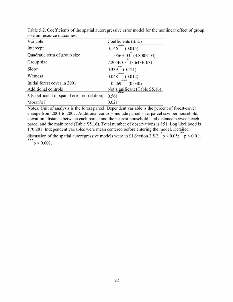
92
Table 5.2. Coefficients of the spatial autoregressive error model for the nonlinear effect of group size on resource outcomes. Variable Coefficients (S.E.)
Intercept 0.146***
(0.015)
Quadratic term of group size – 1.056E-03* (4.800E-04)
Group size 7.205E-03* (3.643E-03)
Slope 0.339**
(0.121)
Wetness 0.048***
(0.012)
Initial forest cover in 2001 – 0.269***
(0.030) Additional controls Not significant (Table S5.16)
λ (Coefficient of spatial error correlation) 0.561***
Moran’s I 0.021 Notes: Unit of analysis is the forest parcel. Dependent variable is the percent of forest-cover change from 2001 to 2007. Additional controls include parcel size, parcel size per household, elevation, distance between each parcel and the nearest household, and distance between each parcel and the main road (Table S5.16). Total number of observations is 151. Log likelihood is 170.281. Independent variables were mean centered before entering the model. Detailed
discussion of the spatial autoregressive models were in SI Section 2.5.2. *p < 0.05;
**p < 0.01;
***p < 0.001.

93
Table 5.3. Path analysis of the two opposing forces through which group size affects collective action.
Path analysis Unstandardized coefficient (S.E.)
Dependent variable: Free rider (binary: 0 for a household that does not free ride; 1 for a household that free rides)
Group size 0.146**
(0.051) Within-group enforcement (binary: 0 for weak enforcement; 1 for strong enforcement) – 0.522
** (0.184)
Dependent variable: Within-group enforcement
Group size 0.103**
(0.038) Within-group division (binary: 0 for no within-group division; 1 for within-group division)
0.376 (0.266)
Group size × Within-group division – 0.050 (0.061)
Dependent variable: Group size
Social ties to local leaders (binary: 0 for weak social ties; 1 for strong social ties)
0.052 (0.651)
Distance to main road (log) – 0.067 (0.136)
Number of laborers – 0.051 (0.350)
Household size 0.027 (0.243)
Education of adults 0.016 (0.117)
Household income (log) – 0.093 (0.311)
Percentage of agricultural income 1.839 (0.946)
Notes: Unit of analysis is the household, but both characteristics of households and their assigned groups are considered. Continuous independent variables are mean centered. All goodness-of-fit indices show that the model fit is respectably high (Table S5.5). Total number of
observations is 113 households. **
p < 0.01.

94
Figure 5.1. Hypothetical effects of free riding, within-group enforcement, and group size on collective action and resource outcomes. Notes: Both free riding and within-group enforcement are hypothesized to be positively related to group size. But free riding is hypothesized to be negatively related to within-group enforcement. The combined effects of free riding and within-group enforcement on collective action and resource outcomes are not expected to be additive because of interactions between within-group enforcement and free riding. The net effect of group size is determined by the dynamics (e.g., strength and variation with group size) of free riding and within-group enforcement, which may form a nonlinear pattern.
Free riding/Enforcement
Free riding EnforcementCollective action/O
utcomes
Group size
Group size

95
Figure 5.2. Map of the location, main road, forest cover in 2007, and household monitoring parcels of Wolong Nature Reserve in Sichuan Province, China.

96
Figure 5.3. The nonlinear group-size effects on collective action and forest outcomes. Notes: This figure shows the predicted monitoring effort (A) and forest-cover change (B) from 2001 to 2007 under different group sizes (i.e., number of households monitoring a single forest parcel). The graphs show the net effects of group size on per household monitoring effort and on change in forest cover, while controlling the other variables in Tables 5.1 and 5.2. The blue line is the predicted fit based on group size, and the orange dots are the actual observations. One dot may represent several overlapping observations. Except for linear and quadratic terms of group size, all other independent variables were controlled as their mean values (Tables S5.1 and S5.3). In B our conclusion still holds as the nonlinear effect is still significant even when excluding the parcels with group size of one, or the two parcels with group sizes of 15 and 16 (see details in SI Section 2.5.2). However, for A and B, the observations do not visually fit the predicted lines in the same way as the observations in ordinary least-squares regressions (Daniel et al., 1999) because these models are not the ordinary least-squares regressions (see details in SI section 2.5).

97
CHAPTER 6
INTERACTION EFFECTS OF CONSERVATION AND DEVELOPMENT POLICIES
ON RURAL HOUSEHOLD INCOME AND INCOME STRUCTURE
In collaboration with
Thomas Dietz, Zhiyun Ouyang, Jianguo Liu

98
Abstract
Numerous conservation and development policies have been implemented
simultaneously around the world, but little attention has been given to how these policies interact
with each other. Using data collected since 1995 in Wolong Nature Reserve, we examined both
the main and interaction effects of conservation and development policies on rural household
income and income structure. Our study confirmed the existence of both synergistic and
antagonistic effects among different conservation and development policies, which are seldom
given much attention to during the design, implementation and/or evaluation of conservation and
development policies. Such interaction effects also led to unanticipated consequences. The
payments from two conservation policies, when examined separately, negatively affected
household income, but jointly led to a positive effect. Our findings suggest that conservation and
development policy studies should use an integrated paradigm by accounting for complex policy
interactions, and jointly designing, implementing, monitoring, and evaluating conservation and
development policies.

99
6.1 Introduction
To mitigate widespread ecosystem degradation and improve human well-being,
numerous conservation and development policies have been designed and implemented and
often there are multiple policies at any given locale. Increasingly, conservation and development
are seen as linked, a point first made by the IUCN in 1980 (IUCN, 1980). Two distinct courses
may characterize such policy intervention efforts. On one hand, conservation policies
increasingly seek to integrate development goals (e.g., poverty alleviation) to gain public support;
on the other hand, development policies seek to incorporate conservation goals under the slogan
of sustainable development (Tallis et al., 2008). Despite the efforts to integrate conservation and
development goals, policies were often evaluated separately and little attention has been given to
how conservation and development policies interact with each other.
Considering the potential interactions among policies is critically important for several
reasons. First, ignoring the interactions of multiple policies may lead to biased estimates of the
effects of each policy. Second, ignoring the interaction effects may lead to strategies that
enhance the performance of one policy but compromise that of another policy, or in some cases,
may lead to failures of both policies. This is a key issue for the recently popular payments for
ecosystem services (PES) programs because payments for protection of one service may affect
the provision of other services(Foley et al., 2005; Kareiva et al., 2011; Kinzig et al., 2011;
Millington et al., 2013; Nelson et al., 2009). Third, for policies with dual or multiple goals such
as the Integrated Conservation and Development Programs (ICDPs), there could also be
interaction effects among different policy implementation strategies. The pervasive failures of
ICDPs are in part largely due to lack of understanding such complex interactions (Liu et al.,
2007a; Liu et al., 2013). Fourthly, different policies may interact with each other, form feedback

100
loops, and generate unanticipated or unintended consequences and these effects may differ
across scales. A program to construct efficient irrigation infrastructure (e.g., drip irrigation)
decreased water use on individual farms but increased evapotranspiration (i.e., loss of water
associated with plant use), reduced groundwater recharge, and redistributed water supply at a
water basin scale, which increased overall water use at large scales and affected distant holders’
water rights (Ward and Pulido-Velazquez, 2008). Providing incentives for more efficient
irrigation infrastructure alone also cannot guarantee less overall water use (Ward and Pulido-
Velazquez, 2008). Only the combination of the two policies with other institutional innovations
that account water use at multiple scales may reduce overall water use (Ward and Pulido-
Velazquez, 2008). Finally, in every location on the globe, there are concurrent conservation
and/or development policies being implemented at local, regional to national and global scales
(Liu and Yang, 2012). While in some cases a single policy may be the major driver of social and
environmental change, in most cases the influence of interaction effects of multiple policies
cannot be dismissed without careful analysis.
Theoretically, the outcome of interactions among different policies can present in any of
the forms shown in Fig. 6.1. [We are aware that besides multiplicative interaction terms there are
other statistic forms of interactions (Blalock, 1965; Southwood, 1978). Here we use
multiplicative interaction terms because they are the most common statistical specification and
well capture the sorts of effects we anticipate (Aiken and West, 1991; Friedrich, 1982; Whisman
and McClelland, 2005).] When the total effect of two policies is greater than the sum of their
individual effects, one will see a synergistic effect (Fig. 6.1a, 6.1c, and 6.1e). On the contrary,
when the total effect of two policies is smaller than the sum of their individual effects, one will
see an antagonistic effect (Fig. 6.1b, 6.1d, and 6.1f). When such different forms of complex
101
interactions are not considered, the outcomes may come as surprises, unanticipated and
unintended consequences (Kinzig et al., 2011; Liu et al., 2007a). While there is some theoretic
discussion of the interaction effects among policies (Liu et al., 2008; Liu et al., 2013), systematic
empirical examinations of the interactions of conservation and development policies are
altogether missing from the current literature.
To fill these knowledge gaps, we used data from a long-term project and extensive local
knowledge at Wolong Nature Reserve in China, where we have worked since 1995, to estimate
both the main and interaction effects of conservation and development policies.
6.2 Methods
In this study we considered the four most important conservation and development
policies implemented in the reserve, where we judge importance in terms of implementation
scale, payment, duration, and potential impacts. Based on their primary goals, here we
considered the Natural Forest Conservation Program (NFCP) and Grain-to-Green/Bamboo
Program (GTGB) as conservation policies and the Electricity Subsidy Program (ESP) and
Tourism Development Program (TDP) as development policies. The general background
information of these four policies is shown in Table 6.1. Because all the four policies have dual
conservation and development goals, which may profoundly affect local households’ livelihood,
dependence on ecosystem services, and thus biodiversity conservation (Adams et al., 2004; Yang
et al., 2013c), here we focus on household income and income structure (i.e., percentage of
agricultural income) as indicators of policy outcomes.

102
We constructed two types of econometric models to examine the main and interaction
effects of conservation and development policies on changes in total household income and
income structure. Controlling other factors, one type of model used the amount of payments or
subsidies; the other used the percentage of income from payments or subsidies (i.e., the
corresponding payment or subsidy divided by the total household income). We presented the
main results from the models using the percentage of payments or subsidies in Tables 6.2 and 6.3.
The complementary results from the models using the amount of payments or subsidies are
shown in Tables S6.2 and S6.3. The descriptive statistics of our data are summarized in
Supplementary Information Table S6.1.
6.2.1 Study area
Wolong Nature Reserve (N 30˚45' – 31˚25', E 102˚52' – 103˚24'; Fig. 6.2) for Giant
Pandas (Ailuropoda melanoleuca), a flagship protected area, is one of the earliest nature reserves
established in China. It is situated in Sichuan Province, Southwestern China, in the transition
between the Sichuan Basin and the Qinghai-Tibet Plateau. It is established in 1963 and expanded
to its current size of 2,000 km2 in 1975. Currently, there are ~4,900 local residents in 1,200
households across two townships (i.e., Wolong and Gengda). It is characterized by a high
variation in topographic, climatic and hydrological conditions with very high level of
biodiversity, supporting the largest wild population of giant pandas (~ 10% of the world’s total)
and over 6,000 other plant and animal species (Schaller et al., 1985). It is identified as one of
China’s first three UNESCO Biosphere Reserves in 1979 (Li and Zhao, 1989), part of the
Southwestern China Mountains biodiversity hotspot in 2000 (Myers et al., 2000), and part of the
UNESCO World Heritage Site — Giant Panda Sanctuary — in 2006 (Liu et al., 2012).

103
Wolong Nature Reserve is also a place that has been experiencing dramatic economic and
environmental transformation since the late 1990s. In the 20th
century, this area was relatively
inaccessible to the outside world and was characterized by a subsistence-based agricultural
economy (Liu et al., 2012). The vast majority of local residents were and are farmers primarily
involving in such agricultural activities as growing maize and vegetables, cultivating livestock
(e.g., pigs, cattle, yaks, and goats), keeping bees, harvesting timber, and collecting non-timber
forest products such as traditional Chinese medicine plants, bamboo shoots, mushrooms and
fuelwood (Yang et al., 2013c; Yang et al., 2013e). During the 1980s, the central government
started to improve infrastructure and construct conservation stations both inside and outside the
reserve (Wolong Nature Reserve, 2005). In early 1980s international collaboration between the
State Administration of Forestry of China and World Wildlife Fund helped to establish the
world’s largest in-captivity panda breeding and research facility in the reserve, the Center for
Research and Conservation of Giant Pandas (CRCGP). International aid from the World Food
Programme of United Nations (US$887,000) from 1984 to 1986 and some matching fund from
the central government further improved local infrastructure and converted 113 ha of cropland
into forest (Wolong Nature Reserve, 2005). By the middle of 1990s the steadily increase of
pandas born in captivity at CRCGP had put the reserve in the international limelight and it
became a global tourism destination. In 1999, a provincial highway connecting the reserve to the
outside was completed and markedly improved the accessibility of this area. The annual number
of tourists had increased from 20,000 in 1996 to 108,100 in 2000, with a peak of 235,500 in 2006,
followed by a valley of 13,000 in 2008 due to the 2008 Wenchan Earthquake (Liu et al., 2012).
However, even during the peak year in 2006, only 24% of local households received direct or

104
indirect benefits from the tourism industry(Liu et al., 2012). As much as 96% of tourism revenue
was obtained by the local government and an outside tourism company (Liu et al., 2012).
Since 2000, in response to the rapid degradation of forest and panda habitat in the reserve
(Liu et al., 2001), several national and local conservation policies were implemented, which also
have important potential socioeconomic impacts. The four most important conservation and
development policies in terms of implementation scale, payment, duration, and potential impacts
are the Natural Forest Conservation Program (NFCP), Grain-to-Green/Bamboo Program
(GTGB), Electricity Subsidy Program (ESP), and Tourism Development Program (TDP; Table
6.1). All the four policies included both conservation and development goals.
6.2.2 Data collection and analyses
In our study area, households are the basic units of decision making for most
socioeconomic activities such as agricultural production, small business operation, local
temporary work, and migrant work as well as for environmentally significant behaviors such as
fuelwood collection, enrollment in GTGB, and forest monitoring for NFCP (An et al., 2001; Liu
et al., 2012; Yang et al., 2013c; Yang et al., 2013e). Therefore, we collected data at the
household level. Usually household heads or their spouses are decision makers who are familiar
with household affairs (An et al., 2001), and thus we chose them as interviewees.
In 1999, our research team conducted the first household survey at Wolong Nature
Reserve to collect data for the year 1998 (An et al., 2001). We conducted stratified random
sampling of 220 households (i.e., ~20% of all the households) based on administrative groups
(an administrative unit under the village level). Since then, we have been maintaining good
collaborative relationship with local governments and communities. Because the overall
education level of local residents is low, we conducted face-to-face interviews using interviewers

105
fluent in the local dialect and accompanied by a local assistant. Our household questionnaires
elicited information of demographic status (e.g., household size, birth year, gender, and
education level), and basic socioeconomic activities (e.g., income, expenditure, and energy use).
In the end of 2007 and early of 2008, we revisited the households sampled in 1999 to
collect data for the year 2007. We were able to re-interview 183 households, of which four
households were excluded from analyses because their household registrations were later
changed to non-rural households and did not qualify for receiving NFCP payment. The losses of
other previously sampled households are due to a diversity of reasons including deaths,
migration to outside areas, divorce, and temporarily working outside the study area during our
survey period. We randomly added 9 other households into the 2007 survey. In addition to
repeating the questions surveyed in 1999, we also asked for information on participation in and
payments from conservation policies (i.e., NFCP and GTGB).
In addition to the household surveys, we also measured the locations of households using
a Global Positioning System device and calculated the distance from each household to the main
road using the software ArcGIS 10.1 (ESRI Inc., California, USA).
6.2.3 Econometric Models
We propose that changes in rural households’ total income and income structure are
determined not only by policy intervention but also by different forms of capital (Li et al., 2011;
Liu et al., 2012) as shown in Eq. 6.1:
Y = β0 + P1 β1 + P2β2 + Cf βf + Ch βh + Cn βn + Cb βb + Cs βs + Cc βc + ε, (6.1)
Where Y is the changes in total household income or changes in the percentage of agricultural
income; P1 is a vector of different policy intervention variables; P2 is a vector of interaction

106
terms of different policy intervention variables; Cf is a vector of indicators of financial capital;
Ch is a vector of indicators of human capital; Cn is a vector of indicators of natural capital; Cb
is a vector of indicators of built-up capital; Cs is a vector of indicators of social capital; Cc is a
vector of indicators of other contextual factors; βis are parameter vectors to be estimated; and ε is
the error term that has a normal distribution with mean of zero.
To improve the interpretability of coefficients and reduce the collinearity among the
linear and interaction terms (Supporting Information [SI] Appendix E, supporting text), all
continuous independent variables were mean-centered prior to their input into the regression
models (Schielzeth, 2010). All the statistical analyses were performed using the software of
STATA 12.0 (StataCorp LP, Texas, USA). Models were estimated via centered polynomial
regression.
6.3 Results
Our results show that NFCP payment percentage and GTGB payment percentage are both
negatively associated with changes in total household income, while the coefficient of their
interaction term is positive and significant (p < 0.001, Table 6.2). These results are consistent
with the form of interaction effect shown in Fig. 6.1e, suggesting an antagonistic effect. As the
results in Table 6.2 are centered polynomial regression (Supporting Information [SI], supporting
text), when all other variables are controlled at their mean values, increasing the NFCP and
GTGB payment percentages by 1% and 1% actually on average reduce the increase in household
income by 1,288 yuan (or 5.9% of the mean value) and 155 yuan (or 0.7% of the mean value),

107
respectively. The coefficient of the interaction between NFCP payment percentage and tourism
participation was negative and significant (p = 0.022, Table 6.2). This is consistent with the form
of hypothesized policy interaction effect in Fig. 6.1d, also indicating an antagonistic effect.
Again, controlling all other relevant variables at their mean values, households participating in
tourism businesses actually on average had 5,274 yuan (or 24.0% of the mean value) more
increase in household income than those did not participate. In addition, the initial electricity
subsidy percentage, increase of agricultural income, number of laborers in 1998, and increase in
the number of laborers all positively contribute to the increase of total household income. But the
initial cropland area and distance from each household to the main road both negatively affect
the increase of total household income (Table 6.2). Additional analyses suggest that households
own more initial cropland or locate further away from the main road are less likely to expand
their income sources such as participating in tourism businesses (Spearman’s ρ = – 0.242, p =
0.001 and ρ = – 0.218, p = 0.003, respectively).
Our results also show that GTGB payment percentage and its interaction term with NFCP
payment percentage are both negatively associated with changes in agricultural income
percentage (p = 0.011 and p = 0.001, respectively), but the coefficient of NFCP payment
percentage is not significant (Table 6.3). These results are consistent with the forms of
interaction effect shown in Fig. 6.1b, indicating a synergetic effect. When all other variables are
controlled at their mean values, increasing the GTGB payment percentage by 1% helps to reduce
agricultural income percentage by 0.3% (or 1.6% of the mean value). The coefficient of the
interaction between NFCP payment percentage and tourism participation was negative and
significant, while neither of their main effects are significant (Table 6.3). These results are still
consistent with the form of hypothesized interaction effect in Fig. 6.1e or Fig. 6.1f, in which the
108
main effects of both policies are not significant while the interaction effect is negative and
significant. In addition, the increase of agricultural income, total area of cropland in 1998, and
the distance from each household to the main road all have positive coefficients, and thus have
negative effects on the reduction of the percentage of agricultural income, while the effects of
initial electricity subsidy percentage, initial percentage of agricultural income in 1998, and social
ties to local governments are opposite in sign.
6.4 Discussion
Our study confirmed the existence of both synergistic and antagonistic effects among
different conservation and development policies, which are seldom given much attention to
during the design, implementation and/or evaluation of conservation and development policies. It
should be noted that it is difficult, if not impossible, to distinguish empirically all the possible
forms of interaction effects in any single study. Rather, the intention of this study is to
empirically substantiate the importance of taking interaction effects into account in policy
research and practice.
Our findings also suggest that synergistic and antagonistic effects not only emerge
between conservation and development policies, but also exist among different conservation
policies or among various development policies. The environmental and socioeconomic
effectiveness and efficiency of different policies often are evaluated separately, thus ignoring
other simultaneously implemented policies (Liu et al., 2008; Yang et al., 2013e). The results of
such evaluations could be biased and misleading. Improved understanding of complex policy

109
interactions may also reverse the currently common failures of ICDPs to achieve both
environmental and socioeconomic sustainability.
Interaction effects lead to unanticipated consequences when the context or underlying
mechanisms are not well understood. In our case, NFCP or GTGB payment percentage
separately led to a negative impact on the changes in total household income, while jointly they
had a positive effect. These results may seem to be surprising but are reasonable if the context is
considered. For households affected only by NFCP or GTGB, the policy impacts might not be
large enough to draw the attention of some households (e.g., NFCP payment accounts for less
than 5% of total household income for 53% of households) or they might adopt incremental
adaptation strategies (Kates et al., 2012) to offset the negative policy impacts. For example,
based on our over 18 years’ local knowledge, to offset the negative impacts of NFCP or GTGB
on their household income, many households adopted incremental adaptation strategies by
adjusting their traditional agricultural activities such as switching from low income crops (e.g.,
corn and potato) to high income crops (e.g., cabbage and traditional Chinese medical plants) and
intensifying agricultural practices (e.g., increasing the use of fertilizers and chemical
pesticides)(Yang et al., 2013c; Yang et al., 2013e). However, for many households who were
both affected by NFCP and GTGP, it might be difficult for them to raise their families with the
small amount of remaining cropland (on average less than 40% of cropland remained) even if
they adopted the incremental adaptation strategies mentioned above. Therefore, they might be
forced to adopt transformational adaptation strategies (Kates et al., 2012) such as substantially
reducing or abandoning agricultural activities and going outside the reserve for migrant work or
business opportunities in cities(Chen et al., 2012a). Such transformational adaptation strategies
increased their total household income (Chen et al., 2012a) but might decrease their well-being

110
because in urban areas they may lack of quality health insurance cover and medical care, face
substantial educational expenses for their children, and experience discrimination from urban
residents, high stress and depression (Wong et al., 2007; Yang et al., 2013a).
In conclusion, our findings emphasize that the design, implementation and evaluation of
conservation and development policies are complex and thus require a systematic and integrated
approach (Liu et al., 2007a; McConnell et al., 2011). To appropriately evaluate the effectiveness
and efficiency of policies and avoid unanticipated or unintended negative consequences,
different conservation and development policies should take the interaction effects into
consideration and should be jointly designed, implemented, monitored and evaluated.

111
Table 6.1. General information of the four conservation and development policies in Wolong Nature Reserve.
Natural Forest Conservation Program (NFCP)
Grain-to-Green/Bamboo
Program (GTGB)*
Electricity Subsidy Program
Tourism Development Program
Aim Protect and restore natural forests through logging ban, afforestation, and payments
Convert cropland to timber or bamboo forests or shrub lands with payments and alleviate poverty
Encourage the switch from use of fuelwood to electricity and improve local livelihood
Provide alternative income sources to local households and generate additional funds for conservation
Type Conservation policy with development goal
Conservation policy with development goal
Development policy with conservation goal
Development policy with conservation goal
Implementation method
Incentive-based mechanism
Incentive-based mechanism
Incentive-based mechanism
Partnership between local government and a tourism company
Initial year 2001 Green-to-Green: 2000; Green-to-Bamboo: 2002
2002 2002†
Duration 10 years (renewed in 2010 for another 10 years till 2020)
8 years (Grain-to-Green: renewed in 2008 for another 8 years; Green-to-Bamboo: ended in 2010)
Continual unless being terminated
Continual unless being terminated

112
Table 6.1 (cont’d) Natural Forest
Conservation Program (NFCP)
Grain-to-Green/Bamboo Program (GTGB)*
Electricity Subsidy Program
Tourism Development Program
Implemented area
120,500 ha of land below treeline (i.e., 3600 m above sea level)
Grain-to-Green: 367.3 ha from 969 households; Grain-to-Bamboo: 81.9 ha from 530 households
Experimental zone of the reserve
Experimental zone of the reserve
Average payment rate
~900 yuan per household per year (almost tripled after
2010)‡
Grain-to-Green: 3600 yuan per ha per year (halved after 2008); Grain-to-Bamboo: 13,500-18,000 yuan per ha per year
0.07 yuan per kilowatt-hour
Not applicable
Notes: * The Grain-to-Bamboo is a local program complementing the Grain-to-Green Program
and attempts to convert cropland to bamboo forests for giant pandas. Due to the similarities in terms of aim and implementation method, together here we viewed them as one integrated cropland returning policy (i.e., GTGB). † Tourism development has been proposed and adopted in Wolong Nature Reserve since 1980s.
But the Ecotourism Development Plan in Wolong Nature Reserve was officially approved by the State Forestry Administration of China in 2002. ‡ As officially announced by the Wolong Administrative Bureau, the payment rate for NFCP was changed from 900 yuan per household per year into 600 yuan per capita since 2011. Only household members with an age of 7 years or above were qualified for head count.

113
Table 6.2. Effects of conservation and development policies on changes in total household income. Variables Unstandardized
coefficients Standardized coefficients
Robust S.E.
Policy intervention NFCP payment percentage
–128.811***
–0.286***
35.194
GTGB payment percentage
–15.535* –0.087
* 7.707
Initial electricity subsidy percentage
63.921* 0.097
* 28.004
Tourism participation
5.274† 0.086
† 3.188
NFCP payment percentage × GTGB payment percentage
387.458***
0.263***
89.473
NFCP payment percentage × Initial electricity subsidy percentage
–188.653 –0.042 133.730
NFCP payment percentage × Tourism participation
–228.758* –0.201
* 98.906
Financial capital Initial total household income
–0.175 –0.032 0.294
Changes in total agricultural income
1.114***
0.633***
0.251

114
Table 6.2 (cont’d) Variables Unstandardized
coefficients Standardized coefficients
Robust S.E.
Human capital Number of laborers
2.767* 0.148
* 1.283
Changes in number of laborers
2.161* 0.143
* 0.977
Education 0.119 0.015 0.407
Natural capital Cropland area –1.451* –0.130
* 0.578
Built-up capital Distance to the main road, log
–1.783**
–0.132**
0.563
Social capital Social ties to local governments (1: yes; 0: no)
0.319 0.004 3.919
Township 1: Wolong; 0: Gengda
4.253 0.078 2.671
Constant 14.601***
— 2.788
Notes: Dependent variable is the change of total household income from 1998 to 2007 (i.e., total household income in 2007 subtracting total household income in 1998). All continuous independent variables were mean-centered before entering the model. The number of observations is 179. The R-squared is 0.728. Variation Inflation Factors (VIFs) were tested to be less than 5. The interaction terms between GTGB payment percentage and initial electricity subsidy percentage, and between GTGB payment percentage and tourism participation were not included to avoid multi-collinearity and biased coefficient estimates. But our conclusions were
consistent regardless of including or excluding these two interaction terms. † P < 0.1;
* p < 0.05;
** P < 0.01;
*** p < 0.001.

115
Table 6.3. Effects of conservation and development policies on changes in agricultural income percentage. Variables Unstandardized
coefficients Standardized coefficients
Robust S.E.
Policy intervention
NFCP payment percentage 0.904 0.141 0.663
GTGB payment percentage –0.347* –0.136
* 0.135
Initial electricity subsidy percentage
–1.218**
–0.129**
0.347
Tourism participation –0.037 –0.043 0.041
NFCP payment percentage × GTGB payment percentage
–3.660**
–0.174**
1.078
NFCP payment percentage × Initial electricity subsidy percentage
4.182 0.066 4.052
NFCP payment percentage × Tourism participation
2.398**
0.148**
0.870
GTGB payment percentage × Initial electricity subsidy percentage
–1.204 –0.020 3.615
GTGB payment percentage × Tourism participation
–0.218 –0.038 0.263
Financial capital Initial total household income 1.14e-03 0.014 3.60e-03
Initial agricultural income percentage
–0.859***
–0.685***
0.055
Changes in total agricultural income
6.86e-03**
0.274**
2.51e-03
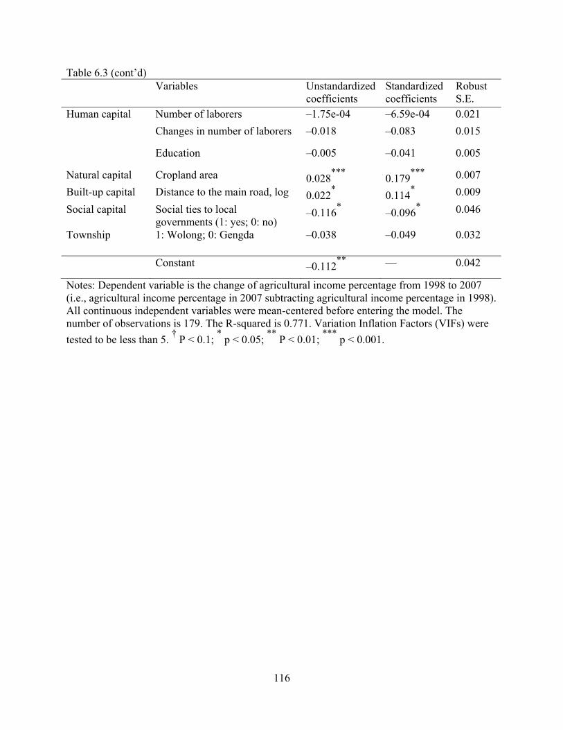
116
Table 6.3 (cont’d) Variables Unstandardized
coefficients Standardized coefficients
Robust S.E.
Human capital Number of laborers –1.75e-04 –6.59e-04 0.021
Changes in number of laborers –0.018 –0.083 0.015
Education –0.005 –0.041 0.005
Natural capital Cropland area 0.028***
0.179***
0.007
Built-up capital Distance to the main road, log 0.022* 0.114
* 0.009
Social capital Social ties to local governments (1: yes; 0: no)
–0.116* –0.096
* 0.046
Township 1: Wolong; 0: Gengda –0.038 –0.049 0.032
Constant –0.112**
— 0.042
Notes: Dependent variable is the change of agricultural income percentage from 1998 to 2007 (i.e., agricultural income percentage in 2007 subtracting agricultural income percentage in 1998). All continuous independent variables were mean-centered before entering the model. The number of observations is 179. The R-squared is 0.771. Variation Inflation Factors (VIFs) were
tested to be less than 5. † P < 0.1;
* p < 0.05;
** P < 0.01;
*** p < 0.001.

117
Figure 6.1. Hypothetical outcomes of interaction effects among different policies. Notes: To simplify the illustration, here we considered interactions between two policies: (a) both policies have positive effects and the interaction effect is also positive; (b) both policies have negative effects and the interaction effect is also negative; (c) one policy has positive effect, another policy has negative effect, and the interaction effect is positive; (d) one policy has positive effect, another policy has negative effect, and the interaction effect is negative; (e) both policies have negative effects but the interaction effect is positive; (f) both policies have positive effects but the interaction effect is negative. Vertical dashed line indicates the initial implementation time of the policies. The blue line indicates the static baseline without policy intervention (although the baseline may not be static, here we used it to simplify the illustration).

118
The orange and red lines indicate positive and negative policy outcomes, respectively. If the effect(s) of one or two policies or their interaction term is (are) not statistically significant, the orange or/and red line(s) will overlap with the no policy line, which is (are) just a special case(s) of the six forms.

119
Figure 6.2. Wolong Nature Reserve in Sichuan Province, southwestern China.

120
CHAPTER 7
PERFORMANCE AND PROSPECTS OF PAYMENTS FOR ECOSYSTEM SERVICES
PROGRAMS: EVIDENCE FROM CHINA
In collaboration with
Wei Liu, Andrés Viña, Junyan Luo, Guangming He, Zhiyun Ouyang, Hemin Zhang, Jianguo Liu

121
Abstract
Systematic evaluation of the environmental and socioeconomic effects of Payments for
Ecosystem Services (PES) programs is crucial for guiding policy design and implementation. We
evaluated the performance of the Natural Forest Conservation Program (NFCP), a national PES
program of China, in the Wolong Nature Reserve for giant pandas. The environmental effects of
the NFCP were evaluated through a historical trend (1965-2001) analysis of forest cover to
estimate a counter-factual (i.e., without-PES) forest cover baseline for 2007. The socioeconomic
effects of the NFCP were evaluated using data collected through household interviews carried
out before and after NFCP implementation in 2001. Our results suggest that the NFCP was not
only significantly associated with increases in forest cover, but also had both positive (e.g., labor
reduction for fuelwood collection) and negative (e.g., economic losses due to crop raiding by
wildlife) effects on local households. Results from this study emphasize the importance of
integrating local conditions and understanding underlying mechanisms to enhance the
performance of PES programs. Our findings are useful for the design and implementation of
successful conservation policies not only in our study area but also in similar places around the
world.

122
7.1. Introduction
Much of the unprecedented degradation of important ecosystem services due to human
activities (MA, 2005) has been explained using the classic ‘tragedy of the commons’ framework
(Hardin, 1968; Jack et al., 2008). However, the landmark work by Elinor Ostrom and
collaborators (Ostrom, 1990; Ostrom, 2009; Ostrom et al., 1999; Ostrom et al., 1994; Ostrom et
al., 2007) challenged this view and suggested that common pool resources can be successfully
managed even without government intervention or privatization. Nevertheless, in many cases
government intervention is still necessary, particularly when local management of common pool
resources does not exist or is ineffective (Jack et al., 2008). Among the different types of
government intervention, payment for ecosystem services (PES) programs have recently
emerged for realigning economic and social costs/benefits among different stakeholders through
incentive-based mechanisms (Chen et al., 2012b; Jack et al., 2008; Scherr et al., 2006). A formal
definition of PES as given by Sven Wunder (Wunder, 2005) as “a voluntary and conditional
transaction over well-defined ecosystem services between at least one seller and one buyer”.
During the past decade, hundreds of PES initiatives have emerged globally (Kalacska et
al., 2008; Liu et al., 2008; Sanchez-Azofeifa et al., 2007; Wunder and Alban, 2008). Among
these, China introduced two of the largest PES programs in terms of scale, total payments and
duration (Liu et al., 2008; Task Force for Eco-Compensation Mechanisms and Polices in China,
2007). Because in many areas participation in these programs is not completely voluntary (Yin,
2009), they may not be regarded as PES programs but rather as PES-like programs. However, for
consistency, in this article we refer to them as PES programs. One of them, the Grain-to-Green
Program (GTGP, also known as the Sloping Land Conversion Program or the Farm to Forest
Program), was initiated in 1999 at the national level to restore natural ecosystems and to mitigate

123
negative off-site effects (e.g., drought, flood, dust storm, sedimentation of reservoirs) caused by
agricultural expansion onto marginal and/or steep land (Liu, 2010; Liu and Diamond, 2005; Liu
et al., 2013). By the end of 2009, GTGP had accumulated an investment of ca. 31.7 billion USD
(1 USD = 6.3 Chinese yuan, May 2012), with averages of 547.6 USD per ha and 381.0 USD per
ha in the upper reaches of the Yangtze River basin and middle-upper reaches of the Yellow River
basin, respectively (Liu et al., 2013). By 2009, ca. 32 million rural households enrolled ca. 8.8
million ha of cropland in the GTGP (Liu et al., 2013). The Natural Forest Conservation Program
(NFCP) aims to conserve natural forests via logging bans and afforestation incentives. By the
end of 2009, the NFCP had accumulated an investment of ca. 14.9 billion USD (Liu et al., 2013).
To date both GTGP and NFCP have been funded entirely by the central and local governments.
However, the GTGP is a direct PES program involving local households, while the NFCP is an
indirect PES program that is operated by local forestry bureaus and seldom engages local
households. Only in very few areas such as in Wolong Nature Reserve for giant pandas, the
decentralization of NFCP implementation and engagement of local households have been
attempted.
While several studies (Chen et al., 2009; Chen et al., 2010; Uchida et al., 2009; Uchida et
al., 2005; Viña et al., 2013; Xu, 2002, 2004) have evaluated the effectiveness and efficiency of
the GTGP, relatively few (Xu, 2002; Yin, 2009) have studied the effectiveness and efficiency of
the NFCP. In addition, to our knowledge no study has evaluated the decentralized
implementation of the NFCP (e.g., participation of local households) and its environmental and
socioeconomic consequences. Moreover, very few previous studies on PES programs anywhere
in the world (Arriagada et al., 2009; Gross-Camp et al., 2012; Scullion et al., 2011) have
addressed their environmental and socioeconomic outcomes simultaneously.

124
Based on more than 30 years of remotely sensed data combined with more than 10 years
of household survey data, in this article we attempt to fill some of these knowledge gaps in the
Wolong Nature Reserve for Giant Pandas. Our objectives are: (1) to evaluate the environmental
outcomes of PES program implementation using a counter-factual without-PES baseline,
estimated using the historical trend of forest cover change; (2) to capture short-term
socioeconomic effects based on empirical data before and after the implementation of the PES
program; and (3) to summarize effective practices and learned experiences, as well as challenges
and opportunities for guiding future conservation policy design and implementation.
7.2. Materials and methods
7.2.1. Study area
We chose Wolong Nature Reserve for Giant Pandas (Ailuropoda melanoleuca) as our
study area not only because it is one of the earliest nature reserves established in China, but also
because it has a relatively independent administrative ability to design and implement its local
PES programs. The reserve is characterized by a high biological diversity and supports
approximately 10% of the total wild giant panda population (Zhang et al., 1997), making it a
flagship reserve not only in China but also around the globe (Liu et al., 2003a).
The Wolong Nature Reserve (N 30˚45’ - 31˚25’, E 102˚52’ - 103˚24’, Fig. 7.1) is located
in Wenchuan County, Sichuan Province, China, in the transition between the Sichuan Basin and
the Qinghai-Tibet Plateau. The reserve is characterized by a high variation in topography (e.g.,
elevations ranging from 1200 m to 6250 m above sea level), soils, climates and hydrological
conditions(Viña et al., 2008). In 1963 (when it was first designated as a nature reserve), its size

125
was around 20,000 ha, but was expanded in 1975 to its current size of approximately 200,000 ha
(Wolong Nature Reserve, 2005). Natural vegetation in the reserve is dominated by four types of
forest, all of which are associated with understory bamboo species: subtropical, evergreen broad-
leaf forests (< 1600 m), evergreen and deciduous broad-leaf forests (1600 – 2000 m), mixed
coniferous and deciduous broad-leaf forests (2000 – 2600 m), and sub-alpine coniferous forests
(2600 – 3600 m) (Schaller et al., 1985; Wolong Nature Reserve, 2005).
In 1983, the State Council authorized the reserve to establish the Wolong Special
Administrative Region with the purpose of protecting regional forest ecosystems and rare plant
and animal species, but primarily for the conservation of the iconic giant panda (Wolong Nature
Reserve, 2005). The establishment of the Wolong Special Administrative Region allowed the
reserve to be a relatively independent administrative entity. Currently, the reserve has two
townships (i.e., Wolong and Gengda), with a total human population of approximately 5700,
including around 4900 local residents that are distributed in approximately 1200 households.
Most local residents are farmers involved in socioeconomic activities such as cultivating maize
and vegetables, raising livestock, collecting medicinal plants, keeping bees, collecting fuelwood,
and cooking animal and human food (Yang et al., 2013c). Fuelwood in the reserve is primarily
used for heating, cooking pig fodder, cooking human food, and smoking pork. It is a local
tradition to raise pigs, smoke pork using fuelwood, and eat smoked pork.
The establishment of the reserve and its expansion in 1975 did not mitigate the
degradation of forest and panda habitat inside its borders (Liu et al., 2001). Therefore, several
PES programs have been designed and implemented. The first one was implemented in 1986
with funds from the World Food Programme of the United Nations, through which 113 ha of
cropland were converted into forest (Wolong Nature Reserve, 2005). Since 2000, two national

126
(i.e., GTGP and NFCP) and one local (Grain-to-Bamboo Program) PES programs have been
implemented in the reserve. Table 7.1 describes general information on these three PES
programs. The three PES programs were designed to target almost all local rural households but
not all households enrolled in those programs (Table 7.1). As opposed to other NFCP
implementation areas in which afforestation practices are also included, the implementation of
the NFCP in the reserve only included forest monitoring activities, targeting all the areas
(approximately 120,500 ha) below the treeline (around 3600 m above sea level) in the reserve.
As a local PES program complementing the GTGP, the Grain-to-Bamboo Program was designed
to increase the bamboo cover (giant panda’s main food) by enrolling cropland located within a
15m buffer zone at each side of the main road (Fig. 7.1). The Grain-to-Bamboo Program has an
annual payment rate of 2142.9 to 2857.1 USD per ha, depending on the distance to the main road
and the cropland production relinquished. With comparison to GTGP, the payment rate of Grain-
to-Bamboo Program is higher because it targets flatter and more productive cropland. To date,
the GTGP and the Grain-to-Bamboo Program have enrolled 367.3 and 81.9 ha of cropland,
respectively. But the total implemented area of GTGP and the Grain-to-Bamboo Program
comprises only 0.37% of the area under the NFCP, thus direct environmental effects of these
programs could be considered almost negligible. However, the GTGP and the Grain-to-Bamboo
Program may induce both direct and indirect socioeconomic effects that should not be ignored
(Chen et al., 2010). Therefore, we took the GTGP and Grain-to-Bamboo Program into account
when specifically examining the social and economic effects of conservation policies on local
households.
Besides the implementation of PES programs, the major economic development in the
reserve during the past two decades has been tourism. A tourism development plan was proposed

127
and adopted as a tool to generate funds for conservation and to provide alternative income
sources for local farmers. While it started in the 1980s, this plan was not fully implemented until
2000 after the successful breeding of captive pandas and the completion of a provincial highway
in the late 1990s (Liu et al., 2012). Thus, while only 4% of the households in the reserve
participated in tourism activities in 1998, this increased to 28% in 2007 (Liu et al., 2012).
Tourism development has grown in tandem with infrastructure development (e.g., road, hotels,
and hospitals) and with government revenue. However, more than 96% of the total tourism
revenue has been retained by the local government and an outside tourism company, limiting the
benefits to local households (He et al., 2008; Liu et al., 2012).
7.2.2. Forest cover dynamics
The dynamics of forest cover in the reserve were obtained from forest cover maps
developed in previous studies (Liu et al., 2001; Viña et al., 2007; Viña et al., 2011). These maps
were developed using data from different satellite platforms (i.e., Corona, Landsat MSS and
Landsat TM) combined with ground-truth data acquired during field work. These maps depict
information on forest cover in the reserve during the years 1965, 1974, 1987, 1994, 1997, 2001
and 2007. Image classification procedures ranged from visual interpretation (Liu et al., 2001) to
unsupervised digital image classification (Viña et al., 2007; Viña et al., 2011) using the
ISODATA technique, an iterative process for non-hierarchical pixel classification (Jensen, 1996).
Overall accuracies of these maps were between 78% and 88% using independent ground-truth
data (Liu et al., 2001; Viña et al., 2007; Viña et al., 2011). These maps included two main land
cover classes (i.e., forest and non-forest). For a detailed description of classification procedures

128
and assessments of map accuracy please refer to the cited studies (Liu et al., 2001; Viña et al.,
2007; Viña et al., 2011).
7.2.3. Focus group, individual and household interviews
To understand planning, implementation, evaluation and decision making processes
involved with the NFCP, we conducted focus group, individual, and household interviews. We
invited eight staff members of the reserve for focus group interviews in 2002, 2007, 2009 and
2010. These people were selected because they were directly participating in the implementation
and evaluation processes of the NFCP. These focus group interviews were organized to discuss
forest monitoring activities before the NFCP, perception toward NFCP benefits and costs, and
problems and challenges during the NFCP implementation. We also had individual discussions
with five officials who were in charge of NFCP planning, implementation, evaluation and
decision making in 2002, 2007, 2009 and 2010. The information obtained from focus and
individual interviews were further verified from published and unpublished governmental
documents as well as through household interviews.
For household interviews, we usually chose the household heads or their spouses as
interviewees because they are the decision makers and are familiar with household affairs (An et
al., 2001). For the household interview before the NFCP, we used data acquired in 1999 (220
households through stratified random sampling, approximately 20% of the total households in
the reserve) from previous studies (An et al., 2002; An et al., 2003) by our research team. Data
after the implementation of NFCP were acquired in 2002 (200 households), 2007 (192
households) and 2009 (207 households). About 170 randomly sampled households were in every
wave across the different years (i.e., panel data). The panel surveys elicited basic information

129
such as demographic status, household socioeconomic activities (i.e., income and expenditure)
and energy use (e.g., fuelwood and electricity). In the 2007 and 2009 surveys, besides basic
information from panel surveys, we also added questions regarding NFCP, GTGP and Grain-to-
Bamboo Program payments, and perceptions toward NFCP implementation. All monetary
measures used in analyses were discounted into constant values in the year 2007.
7.2.4. Local adaptation and implementation of the NFCP
As in Costa Rica (Sanchez-Azofeifa et al., 2007), a national PES implementation
authority exists for the NFCP in China. The annual budget for NFCP implementation in the
reserve was 389,206 USD, of which 380,000 USD and 9206 USD were from the central and
provincial governments, respectively. With assistance from the Forest Inventory and Planning
Institute of Sichuan Province (Fig. 7.2), the Wolong Administrative Bureau designed and
implemented a local NFCP. On the one hand, the administrative bureau intended to reduce
conflicts with local households on forest use and engage them in forest monitoring activities
through economic incentives (i.e., payments). On the other hand, the administrative bureau
hoped that the NFCP payment would compensate the foregone household income sources,
reduce illegal logging and fuelwood collection, and even increase household income by
encouraging households to switch from on-farm to off-farm economic activities. The NFCP
payment rate for each household was fixed across years and was decided based on available
funding from central and provincial governments, excluding administrative and operational costs
(e.g., costs for government patrolling and biannual NFCP evaluations). The administrative
bureau also hoped that the switch from fuelwood to electricity would reduce the pressure on
forests. Before the implementation of NFCP, there were eight small hydropower stations in the

130
reserve with a total capacity of 34 megawatts (Wolong Nature Reserve, 2005). But the electricity
generated from these hydropower stations was mostly exported outside the reserve. To assist the
implementation of NFCP and promote the switch from fuelwood to electricity, local power grids
were upgraded and a so-called ecological hydropower station with a total capacity of 1600
kilowatts was constructed in 2002. This ecological hydropower station compensated the
electricity price for local households by 0.01 USD per kilowatt-hour, leading to an actual unit
residential electricity price of 0.03 USD per kilowatt-hour (Wolong Nature Reserve, 2005).
Finally, an integrated local program of NFCP was implemented, which included the logging ban,
payments for household participatory forest monitoring activities, upgrading of rural power grids,
compensation for electricity price, and the establishment of forestry police force to enhance
policy enforcement.
Approximately 40,100-ha forest (about one third of the total implementation area in the
reserve) was assigned to around 1130 households, with an annual average payment rate of
approximately 143 USD per household (Table 7.1), while the remaining area was monitored by
the staff of the Wolong Administrative Bureau. Initially, the Wolong Administrative Bureau
attempted to assign a single forest parcel to each household. However, this approach turned out
to be very difficult to implement because of the difficulty in clarifying forest parcel boundaries.
Therefore, the Bureau finally decided to assign large forest parcels, defined using natural
boundaries (e.g., rivers, ridges, valleys), to groups ranging in size from 1 to 16 households
(Yang et al., 2013f). Of the 40,100 ha of forest assigned to household monitoring activities,
around 16,700 ha were assigned to individual households while the remaining areas were
assigned to groups with two or more households. Through this approach, a household-group
monitoring approach was created which binds households together for forest monitoring
131
activities. Each household in a group shared the same monitoring responsibility and received the
same amount of payment as other household members. The Bureau evaluates the performance of
household forest monitoring activities through biannual field assessments of illegal activities
(e.g., logging, hunting, mining, grazing in restricted areas, collection of seeds and bamboo shoots,
and other activities considered to negatively affect soils, wildlife and natural vegetation) using a
score-based quantitative evaluation standard for deducting payments. All local residents are
encouraged to report illegal activities and will be rewarded in cash by the Bureau. If any illegal
activity is detected in a forest parcel, all households in its corresponding group will have the
same amount of payment deduction, unless they identify the culprits of the illegal activity to the
Bureau (Yang et al., 2013f).
7.2.5. Baseline for environmental benefits
A fundamental question of any PES program is its ability to address “additionality” (i.e.,
difference in ecosystem services provision between the with-PES scenario and a without-PES
baseline). In other words, is the additionality sufficiently large to warrant implementation of a
particular PES program (Wunder, 2007)? To answer this question it is necessary to first identify
a counterfactual without-PES baseline scenario. Such counterfactual scenario may take any of
three forms: static, deteriorating, or improving (Wunder, 2007), which are difficult to identify if
the PES program is already operational. However, it can be approximated using historical trends
involving time periods before PES program implementation, analyzing changes in similar
without-PES study areas (e.g., adjacent sites) or analyzing changes in larger regions or
administrative entities such as using entire countries as a baseline for local PES program
implementations (Kalacska et al., 2008). In this study we chose to analyze the historical trend of

132
forest covers from 1965 to 2001 in the reserve to estimate the without-PES baseline in 2007.
This is a common approach used by the REDD and REDD+ (Reducing Emissions from
Deforestation and forest Degradation, conservation, sustainable forest management and
enhancement of forest carbon stocks) program (FONAFIFO et al., 2012; Olander et al., 2008).
We chose this approach for two main reasons. First, because NFCP is a national conservation
policy, it was impossible to select appropriate without-PES baseline from similar study sites or
use larger regional or administrative entities (e.g., all of China). Second, before the local
implementation of NFCP in 2001, forest dynamics in the reserve showed a deteriorating trend
from 1965 to 2001 (Liu et al., 2001; Viña et al., 2007) while China overall had been
experiencing forest gains since the middle of 1980s (State Forestry Administration of China,
2005). In addition, we acknowledge that the rapid socioeconomic development since the 1990s
would also contribute to reduce the pressure on forests. But it should be noted also that external
impacts (e.g., socioeconomic development) on the reserve had existed since 1961, particularly
with the construction of unpaved roads and had become more intensive since 1992 with the
construction of paved roads (Wolong Nature Reserve, 2005). Thus, the historical trend in forest
cover already included part of these macro-socioeconomic impacts.
Other synchronous factors such as the GTGP implementation and tourism development
may have interaction effects with NFCP on forest cover change. However, the GTGP only
accounts for a very small percentage (< 1%) of the total land area of the reserve (Wolong Nature
Reserve, 2005) and few local households have directly participated in, and benefited from,
tourism related activities (He et al., 2008; Liu et al., 2012). Therefore, these factors were not
likely to be a major driving force of land cover change in the reserve. Moreover, the main
activities responsible for deforestation in the reserve (i.e., logging and fuelwood collection) have

133
been reduced due to the implementation of NFCP (see Section 3.2 below). Our previous studies
(Tuanmu, 2012; Viña et al., 2011; Yang et al., 2013f) also suggest that the NFCP has been a
major driving force of forest change in the reserve and surrounding areas since 2001. Viña et al.
(2011) indicated that NFCP together with GTGP led to the forest transition in Wenchuan County,
from a net forest loss in 1990s to a net forest increase from 2001 to 2007. Tuanmu (2012)
suggested that controlling for other confounding factors different NFCP monitoring approaches
and payment rates in different areas caused different change rates of panda habitat (of which
forest is an essential component) across space. Yang et al. (2013b) showed that different NFCP
monitoring efforts of household groups led to varied changes in forest cover. Therefore, using
the historical forest trend from 1965 to 2001 to estimate the forest area in 2007 as a without-PES
baseline constitutes a reasonable approximation for evaluating the additionality of the NFCP
implementation. However, as the reserve adopted the integrated NFCP implementation approach,
the NFCP additionality evaluated should be attributed not only to the NFCP but also to other
auxiliary measures (i.e., logging ban, upgrading of rural power grids, compensation for
electricity price, and the establishment of forestry police force to enhance policy enforcement).
7.3. Results
7.3.1. Environmental effects of the NFCP implementation
Implementation of the NFCP seems to have reduced illegal logging and increased forest
cover in the reserve (Fig. 7.3 and Fig. 7.4a). All stakeholders in the focus group, individual and
household interviews shared the opinion that illegal logging activities were reduced largely in
response to the NFCP.

134
The equation of historical forest trend from 1965 to 2001 for linear extrapolation of without-PES
baseline in 2007 is given as:
Y = – 857.74X + 1.79E-6 R2 = 0.94 (7.1)
where Y is the area of forest cover (ha), and X is year.
An increase in forest cover is evident post-NFCP implementation. The with-PES forest
cover in 2007 was significantly higher than the estimated without-PES forest cover in 2001 (p <
0.05, Fig. 7.3). Before NFCP implementation, total forest cover decreased from approximately
106,000 ha in 1965 to around 70,000 ha in 2001, while it recovered to approximately 79,000 ha
in 2007. Based on forest cover dynamics between 1965 and 2001, the estimated without-PES
baseline for 2007 was approximately 68,000 ha. Therefore, the additionality of the PES program
between 2001 and 2007 might be estimated as around 11,000 ha, which accounts for roughly
5.5% of the total land area in the reserve.
Due to the differences in accuracy of land cover maps and other synchronous interaction
effects (e.g., effects of GTGP, tourism development), the approximately 11,000 ha gain in forest
cover cannot be completely attributed to the NFCP. However, it constitutes a reasonable
estimation of the additionality, particularly because of the lack of other major drivers of land
cover change and of the observed transition from forest loss before NFCP to forest gain after
NFCP implementation (See Section 2.5). From 2001 to 2007, the cumulative financial NFCP
investment in the reserve by the central and provincial governments was 2.8 million USD
(Wolong Nature Reserve, 2005). Considering only this direct investment and excluding indirect
investments (e.g., tourism development, donations to conservation), the cost-effectiveness ratio
might be estimated as around 254.5 USD per ha of forest gained.

135
7.3.2. Socioeconomic effects of NFCP implementation
The implementation of the NFCP may be triggering not only environmental but also
socioeconomic effects. While many effects may not be measurable in the short term, some short-
term effects are conspicuous and could be associated with the NFCP implementation. For
instance, a shift in the use of different energy sources (i.e., from fuelwood to electricity) was
conspicuous shortly after NFCP implementation. The amount of electricity consumption per
household doubled, while the amount of labor force spent in collecting fuelwood almost halved
after NFCP implementation (Table 7.2). In addition, the energy source for cooking and heating
shifted significantly from high reliance on fuelwood to electricity, while the number of months
using fuelwood for cooking pig fodder also decreased. Given that the energy use shift from
fuelwood to electricity occurred shortly after NFCP implementation but before the upgrading of
rural power grids and the completion of the ecological hydropower station, this shift was most
likely caused by other measures (i.e., the logging ban and payments for forest monitoring) in the
integrated NFCP implementation approach. Finally, no significant relation between household
income and labor force spent in fuelwood collection was found (Pearson’s r = 0.783, p > 0.1).
Combined, these results suggest a general pattern of switching from fuelwood to electricity
irrespective of household economic status.
On average, total household income doubled from 1998 to 2001 and quadrupled from
1998 to 2007. Most (i.e., 89%, N = 183) interviewed households reported that the NFCP had
brought more benefits than costs to them. Overall household perception is that the
implementation of NFCP provided payment, improved environmental quality, prevented water
and soil erosion, landslides, and promoted tourism development (Fig. 7.4a). However, negative
136
effects brought by the NFCP implementation were also reported. The most reported issue was
the restriction on forest use (Fig. 7.4b). Interviewees claimed that their ancestors lived in the
region for hundreds of years before the establishment of the reserve. For several generations they
have depended on forest resources (e.g., timber, wildlife for hunting, fuelwood, traditional
Chinese medicinal herbs, mushrooms, bamboo shoots, and other non-timber forest products).
The NFCP implementation has inhibited many of these activities, and thus cultural traditions and
customs (e.g., using fuelwood to cook pig fodder, smoking pork with fuelwood, and eating
smoked pork) have been affected. Other complaints include the difficultyin collecting fuelwood,
as 80% of the 183 interviewees reported that they had to search a larger area to collect fuelwood
due to the logging ban established by the NFCP (Fig. 7.4b). Almost all households incurred
wildlife-induced losses with different damage rates, although not all of them attributed such
losses to the NFCP implementation. Approximately 65% of the 183 interviewees claimed that
wildlife-induced losses (e.g., loss of crops and livestock due to wildlife predators such as wild
boars, hog badgers, bears, and monkeys) have significantly increased after the NFCP
implementation (Fig. 7.4c). Approximately 89% of the 183 interviewees were unsatisfied or very
unsatisfied with government inaction (i.e., no measures to reduce wildlife-induced losses or no
compensation for wildlife-induced losses) (Fig. 7.4d).
7.4. Discussion
Before the NFCP implementation, the reserve suffered ecological degradation in the form
of deforestation and giant panda habitat losses (Liu et al., 2001). Unlike many other areas in
China, the implementation of NFCP in the reserve engaged various stakeholders and developed a
local program that integrates a logging ban with payments for monitoring activities and included

137
multiple auxiliary measures (i.e., upgrading of rural power grids, compensation for electricity
price, and the establishment of forestry police force to enhance policy enforcement).
Environmental and socioeconomic outcomes of the NFCP implementation were mixed, having
both positive and negative outcomes.
While an increase in forest cover was observed in association with the implementation of the
NFCP, it should be mentioned that little information is currently available for the entire reserve
on the species composition of these areas of forest gain. Field observations have shown that
some of these areas seem to be dominated by exotic and potentially invasive fast-growing
species (e.g., Japanese larch, Larix kaempferi). However, previous studies have shown that giant
pandas and other native wildlife species including the Asiatic black bear (Ursus thibetanus) used
some of these areas (Bearer et al., 2008) , suggesting that secondary forests may also provide
habitat for wildlife species and thus facilitate biodiversity conservation. In addition, the overall
giant panda habitat suitability has increased, particularly in NFCP implementation areas
(Tuanmu, 2012), suggesting that some of the forest areas restored have in fact become suitable
habitat for the pandas. Therefore, while the environmental benefits obtained from the increase in
forest cover associated with the NFCP seem to be spatially heterogeneous, overall they seem to
be positive, at least in terms of habitat restoration for some wildlife species.
The effects of different conservation and development policies on changes in total
household income were also mixed. Results from econometric models developed by our research
group (Yang et al., 2013d) suggest that GTGP and Grain-to-Bamboo Program payments, initial
electricity subsidy, and tourism participation had positive effects on changes in total household
income from 1998 to 2007, respectively. With all other variables controlled at their average
values, a 1% increase of total GTGP and Grain-to-Bamboo Program payments, or a 1% increase

138
of initial electricity subsidy would on average increase the total household income by 2% and
0.04%, respectively. Ceteris paribus, households participating in tourism activities on average
had a 54% higher increase of total household income than those that did not participate. However,
only less than 28% of the households participated either directly or indirectly in tourism
activities. Meanwhile, NFCP payment did not have a significant effect on changes in total
household income from 1998 to 2007 (p > 0.1), while the interaction term between NFCP
payment and tourism participation had a negative effect (p < 0.05). The drastic increase in total
household income from 1998 to 2007 was largely due to selling agricultural produce (e.g.,
cabbages) outside the reserve, conducting local or migrant labor, and participating in tourism
(Liu et al., 2012; Yang et al., 2013d).
Below we summarize some of the lessons learned through the NFCP implementation in
the reserve, as well as some challenges and opportunities.
7.4.1. Lessons learned through NFCP implementation
Several reasons were given by the interviewed households for the significant reduction in
forest cover losses (multiple response question), among which decentralization of monitoring
activities to households (44% of 174 respondents) and payment for forest monitoring activities
(40% of 174 respondents) were ranked as the two most important. Other reasons, such as the
upgrading of rural power grids and subsidies on electricity, were also highlighted as important in
reducing forest cover losses. The introduction of the forest police team for enhancing NFCP
enforcement was also regarded as an important contributor to the reduction in forest cover losses.
Such vigorous local enforcement has also been shown effective in other PES programs in

139
Ecuador (Wunder and Alban, 2008) and in several other places around the world (Chhatre and
Agrawal, 2008). Vigorous local enforcement efforts together with decentralization of monitoring
activities stimulate greater participation and cooperation of service providers by curtailing
expected returns from alternative illegal forest uses, hence render participation in PES programs
more attractive (Chhatre and Agrawal, 2008).
The decentralization of forest monitoring to households complemented previous
command-and-control measures. This decentralization encouraged the participation in, and
compliance with, forest conservation policies. A previous study by our research group has found
that panda habitat (for which forest cover is essential), recovered faster in household monitored
parcels than in government monitored parcels, after controlling for other contextual factors (e.g.,
elevation, slope, aspect, distance to the main road) (Tuanmu, 2012). We have also found that the
effects of group size (i.e., the number of households for monitoring a forest parcel) on household
monitoring efforts and forest outcomes are nonlinear, with intermediate group size (i.e., 9 in a
range from 1 to 16 households) performing the best (Yang et al., 2013f). The optimum group
size also shifts with context. These results confirm the point of no ‘panacea’ or no ‘one-size-fit-
all’ approach for successful management of common pool resources (Ostrom, 1990; Ostrom,
2009; Ostrom et al., 1999; Ostrom et al., 1994; Ostrom et al., 2007), and explain why the practice
of household-group monitoring in the reserve turned out to be quite effective. On the one hand,
with smaller group sizes, households tend to free ride (i.e., do not participate in forest monitoring
activities), particularly if there are inadequate punishment measures within the group. On the
other hand, as group size increases, a household would face increasing pressure of deteriorating
social relationships with other households in the group, and thus would be less likely to free ride
(Yang et al., 2013f). Our previous study (Yang et al., 2013f) confirmed these two opposing

140
effects of group size and the balance between them led to the observed nonlinear response.
However, such mechanisms were not considered by the corresponding policy makers during the
initial NFCP design process. The decentralization and group size formation, although successful,
were more random than planned. Therefore, for guiding future policy design and implementation
it is essential to first consider the mechanisms underlying the potential success or failure of
particular policy prescriptions.
The synchronous reduction of fuelwood consumption, increase of electricity consumption,
and decrease of labor force for fuelwood collection activities shortly after the NFCP
implementation and before the upgrading of rural power grids and the completion of the
ecological hydropower station suggest that the logging ban and payments for forest monitoring
were the most likely candidates in reducing the pressure on forests. Later, upgrading rural power
grids and the ecological hydropower station may have also contributed to the reduction of
logging and forest recovery. Such an upgrade combined with subsidies for electricity use
provided an alternative energy source that simplified the switch from fuelwood to electricity.
This suggests that auxiliary measures offering alternative livelihoods are essential for the
successful implementation of PES programs. Rather than relying on command-and-control
measures, service buyers should then guide and facilitate service providers to change
environmentally harmful behaviors with alternative solutions.
The integration of quantitative evaluation standards with the PES incentive and
punishment mechanism served as a rigorous and sinewy gate guard for policy enforcement. The
essential difference between this evaluation approach and previous approaches was the emphasis
on performance-based measures complementing with command-and-control measures. This
specifically involved the design and execution of an evaluation criterion aimed at assessing the

141
outcomes of the NFCP implementation rather than the processes or procedures for household
forest monitoring. Meanwhile, all the outcomes were linked with the incentive and punishment
mechanisms (i.e., PES distribution and relevant law enforcement). Without this integrated
evaluation approach, the motivation for regular voluntary forest monitoring by households may
largely diminish, as penalties would not be effectively executed. Without this performance-based
evaluation measures the PES program may have been ineffective.
7.4.2. Challenges and Opportunities
The overall environmental and socioeconomic performances of the NFCP in the reserve
were mixed and there were still some unresolved questions. For instance, could the PES program
be more effective or efficient? Was it ethical to achieve conservation goals with the
socioeconomic costs on local communities? Here we argue that the PES program could be
conducted in a more effective, efficient, ethical and sustainable manner.
First, fundamental questions on PES are, to whom, and how much should be paid? From
an efficiency perspective, only those who constitute a credible threat to ecosystem services
provision should be in the scope of a PES program (Wunder, 2005). But this perspective may be
unfair to those who do not threaten ecosystem service provision. However, those who do not
threaten the provision of ecosystem services usually do not have opportunity costs from foregone
environmentally harmful activities (e.g., logging) and may even obtain benefits due to the
externality of ecosystem service provision. As pointed out by Wunder (2005), “the ideal
ecosystem service seller is, if not outright environmental nasty, then at least potentially about to
become so”. The current NFCP payment rate in the reserve was designed in the year 2001 as a
flat payment, which is becoming less attractive because of inflation and increasing opportunity

142
costs. Thus, ideally those who do not or potentially will not be involved in any threatening
deforestation activities should not be included in the NFCP. Even with a fixed budget, savings
from the reduction of participants may be used to appropriately increase payment rates, to make
them more attractive and competitive. However, it is necessary to first develop strategies for
targeting an optimal pool of participant households, while keeping the selection of participants
voluntary, objective, and transparent. Theoretically, such targeting strategies and payment levels
should be jointly designed to maximize environmental benefits with a given budget (Alix-Garcia
et al., 2008; Wunscher et al., 2008). Lessons and experience on designing targeting strategies
(e.g., inverse auction systems) and payment programs (e.g., discriminative payment levels) may
be learned from studies not only in this region (Chen et al., 2010; Viña et al., 2013) but also from
other regions (Alix-Garcia et al., 2008; Uchida et al., 2005; Wunscher et al., 2008).
Second, diversified funding would be critical for sustainable management of the PES
program. Theoretically, there are five basic types of service buyers, who respond to different
motivations (Scherr et al., 2006), including: (1) philanthropic buyers motivated by non-use
values; (2) public sector buyers (e.g., governmental administrations at different scales); (3)
private businesses, organizations or communities who engage in private deals to secure use
values or other business benefits; (4) private buyers who are under regulatory obligation to offset
environmental impacts, and (5) consumers of eco-certified products and services. The current
NFCP implementation is dominated by the form of public sector buyers (i.e., government
compensation mechanism), which currently exhibit the greatest expectations for many sectors in
China (Task Force for Eco-Compensation Mechanisms and Polices in China, 2007). However, as
it is widely accepted, government compensation mechanisms have limitations that are difficult to
overcome, including the lack of elasticity, difficulty in defining payment rates, high operational

143
costs, and excessive governmental fiscal pressure, among others (Liu et al., 2008; Task Force for
Eco-Compensation Mechanisms and Polices in China, 2007). Currently, except through PES
programs, many non-market ecosystem services (e.g., water purification, carbon sequestration)
are being consumed but are not being paid for (Jack et al., 2008; Yang et al., 2008). Thus, to
secure financial sustainability of current and future PES programs, both public and private funds
should be engaged. In the reserve, for example, hydropower companies in the basin provide a
small compensation amount for the electricity they produce but they should provide more funds
since they directly benefit from the service of water conservation provided through the
conservation of forests. Tourism companies should also pay for the direct benefits they receive
through ecotourism and recreation activities in the reserve.
Third, there is a continuous challenge to improve the human well-being of local
households (Yang et al., 2013a) with minimal interference to their local traditions and customs.
The economic conditions of local households are still at a low level and many are still struggling
to maintain basic livelihoods. Therefore, on the one hand, local households should be guided to
find alternative income sources and increase their total income. Currently, agricultural income is
the major economic source for most of the local households and is vulnerable to natural disasters
(e.g., rainstorms, mountain torrents, landslides). The relatively small amount of subsidies
received from various PES programs is not, neither now nor in the foreseeable future, the main
income source for local households. But since the reserve is famous worldwide as the home to
the endangered giant panda, it provides great opportunities to engage academic institutions, non-
governmental organizations and industrial enterprises at different scales to meet local needs. For
instance, current ecotourism and recreation activities in the reserve are largely directed by
tourism development companies while local communities obtain few or no benefits (He et al.,

144
2008; Liu et al., 2012). The spontaneously emerged “Happy Farmer’s House” tourism and other
potential solutions that are adaptive to local conditions (e.g., cultivation of traditional Chinese
Medicine, eco-certified products, and multiple uses of forests, especially non-timber forest
products) and that bring direct benefits to local households could also be important alternative
solutions to consider (Liu et al., 2012). On the other hand, it is important to improve the quality
of local elementary and high-school education (Liu et al., 2003b; Liu et al., 1999a; Liu et al.,
1999b), the quality of local medical care, and social relations among households and between
households and the local government (Yang et al., 2013a), all of which are essential components
of human well-being (MA, 2005).
Finally, both short- and long-term socioeconomic effects related to the PES program and
interaction effects among various policies (Liu et al., 2008) should be addressed. Whereas some
studies in other areas (Daniels et al., 2010; Uchida et al., 2009) have discussed environmental
and socioeconomic effects of PES programs, they are mostly scattered, fragmented, short term
and opportunistic (Liu et al., 2008). In the reserve, although this study captured some short-term
effects, many consequences are neither well-understood nor seriously tackled during the decision
making processes. For instance, wildlife-induced losses (e.g., crop raids) are becoming a
prevalent phenomenon throughout many protected areas in China due to the recovery of wildlife
habitat and increase of wildlife population after the implementation of conservation policies (Cai
et al., 2008; Liu et al., 2013; Zhang and Wang, 2003). However, to date, there are no policies or
regulations to address such human-wildlife conflicts, since conservation needs mostly
overwhelm personal and property rights in protected areas. It should be then emphasized that
taking the socioeconomic effects related to the PES program into consideration is not only an
ethical issue but also it is critical for the sustainability of current and future PES programs.

145
7.5. Conclusions
At the local scale, the PES program seems to have been responsible for most of the
observed increase in forest cover in the reserve. Nevertheless, it had also induced some
socioeconomic effects to local households such as impacts on local livelihoods, increasing
wildlife-induced losses, and threats to local culture, traditions and customs. Many other short-
and long-term effects as well as interaction effects with other conservation and development
policies are largely unknown at this moment.
Lessons learned from this case study emphasize the importance of integrating local
conditions as well as the need for understanding underlying mechanisms into the design and
implementation of PES programs for their successful and sustainable performance. In the reserve,
the successful performance of the NFCP included a combination of decentralization of forest
monitoring activities to households, enforcement efforts, integration of PES with other auxiliary
measures, and the emphasis on performance-based measures complementing command-and-
control measures. Key issues regarding the effectiveness, efficiency, ethics, and sustainability of
current and future PES programs include adaptation of the policy cycle, identification, selection
and engagement of potential beneficiaries and benefactors, appropriate and effective incentive
and punishment mechanisms, diversity and security of financial sources, alternative income
sources for local residents, and solutions for short- and long-term negative socioeconomic effects.
Conservation policy planning and implementation are complex processes. Future
interdisciplinary studies are needed to disentangle underlying complexities such as heterogeneity
across space, time and PES targeting agents, complex interactions of driving forces, contextual

146
effects, reciprocal effects and feedback loops between human and natural systems. As a global
conservation hotspot, the Wolong Nature Reserve for giant pandas acts as a flagship both for
China’s and global conservation practice. Lessons learned in the Wolong Nature Reserve may
also guide policy design and implementation in many other places across China and around the
world.

147
Table 7.1. General information about the PES programs in Wolong Nature Reserve. Item Natural Forest
Conservation Program (NFCP)
Grain-to-Green Program (GTGP)
Grain-to-Bamboo Program
Beginning date 2001 2000 2002
Duration 10 years (renewed in 2010 for another 10 years till 2020)
8 years (renewed in 2008 for another 8 years)
8 years (ended in 2010)
Legal mechanism National conservation policy
National conservation policy
Local conservation policy complementing the GTGP
Targeted area Forest parcels near household locations along the main road
Cropland with slopes larger than 25 degree, which are around household locations
Cropland within the 15 meters buffer zone at each side of the main road
Targeted households
1130 rural households† All 1200 rural households All 1200 rural households
Implemented area All land below treeline (i.e., 120,500 ha and 3600 m above sea level), of which 40,100 ha were assigned for household monitoring
367.3 ha from 969 households
81.9 ha from ~530 households
Average payment
rate*
~143 USD per household per year
~571 USD per ha per year
2143 to 2857 USD per ha per year
Source: Wolong Administrative Bureau; * household interviews, 1 USD = 6.3 Chinese yuan as
of May 2012. † About 70 households were excluded because their household heads or their spouses have non-
rural household registration and thus they were not regarded as local rural households.
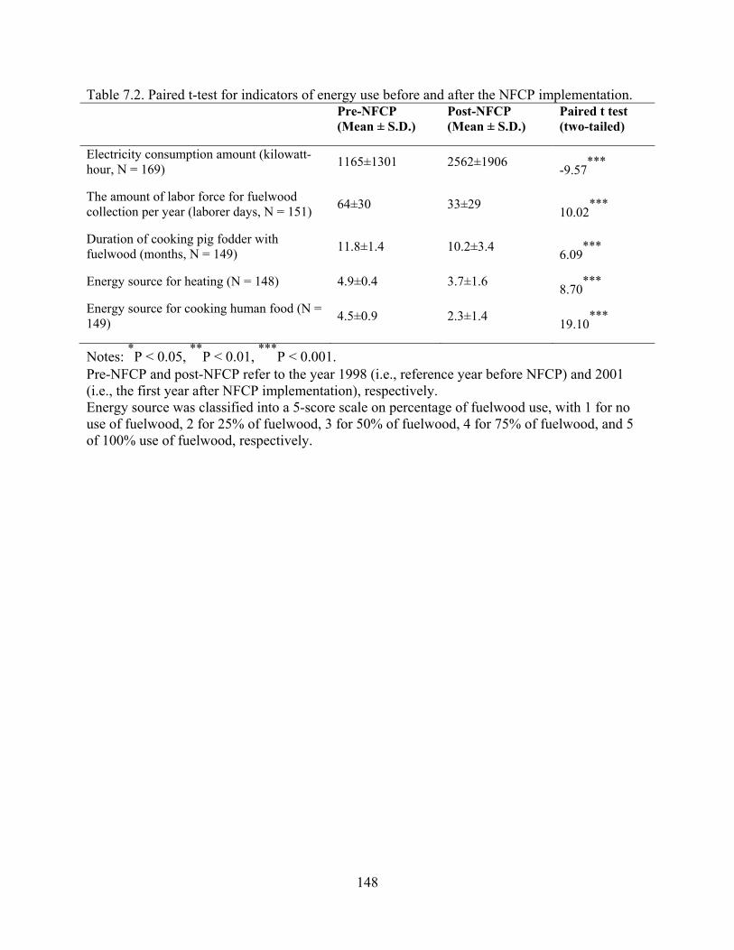
148
Table 7.2. Paired t-test for indicators of energy use before and after the NFCP implementation.
Pre-NFCP (Mean ± S.D.)
Post-NFCP (Mean ± S.D.)
Paired t test (two-tailed)
Electricity consumption amount (kilowatt-hour, N = 169)
1165±1301 2562±1906 -9.57
***
The amount of labor force for fuelwood collection per year (laborer days, N = 151)
64±30 33±29 10.02
***
Duration of cooking pig fodder with fuelwood (months, N = 149)
11.8±1.4 10.2±3.4 6.09
***
Energy source for heating (N = 148) 4.9±0.4 3.7±1.6 8.70
***
Energy source for cooking human food (N = 149)
4.5±0.9 2.3±1.4 19.10
***
Notes: *P < 0.05,
**P < 0.01,
***P < 0.001.
Pre-NFCP and post-NFCP refer to the year 1998 (i.e., reference year before NFCP) and 2001 (i.e., the first year after NFCP implementation), respectively. Energy source was classified into a 5-score scale on percentage of fuelwood use, with 1 for no use of fuelwood, 2 for 25% of fuelwood, 3 for 50% of fuelwood, 4 for 75% of fuelwood, and 5 of 100% use of fuelwood, respectively.

149
Figure 7.1. Map of the Wolong Nature Reserve.

150
Figure 7.2. Natural Forest Conservation Program (NFCP) implementation in the Wolong Nature Reserve (WNR).

151
Figure 7.3. Forest cover area before and after the Natural Forest Conservation Program (NFCP) implementation in 2001. Notes: The historical forest cover trend from 1965 to 2001 was used to estimate the counter-factual without PES baseline in 2007. Additionality is the difference between the with-PES outcome and the without-PES baseline.
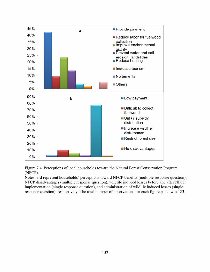
152
Figure 7.4. Perceptions of local households toward the Natural Forest Conservation Program (NFCP). Notes: a-d represent households’ perceptions toward NFCP benefits (multiple response question), NFCP disadvantages (multiple response question), wildlife induced losses before and after NFCP implementation (single response question), and administration of wildlife induced losses (single response question), respectively. The total number of observations for each figure panel was 183.

153
Fig. 7.4 (cont’d)
154
CHAPTER 8
DYNAMICS OF HOUSEHOLD CAPITAL IN PROTECTED AREAS DURING POST-
DISASTER RECONSTRUCTION
In collaboration with
Zhiyun Ouyang, Thomas Dietz, Wei Liu, Jianguo Liu

155
Abstract
Post-disaster reconstruction is often assumed to recover natural, human, manufactured,
and social capitals. However, due to the lack of pre-disaster data, there have been relatively few
systematic evaluations of this proposition. Using long-term household survey data from Wolong
Nature Reserve (an area of global importance in China) and surrounding areas, our results
suggest that the effects of post-disaster reconstruction efforts can differ from one scale to another.
After five years’ reconstruction, the overall capital at the reserve level is improving with the
huge amount of reconstruction investment, but there was an overall deterioration of household
capital both inside and outside the Reserve. Such deterioration is partly due to associated
disasters after the earthquake and partly due to inappropriate management. Our findings suggest
that capacity building and recovery should not be taken for granted in post-disaster
reconstruction and require integrated planning and implementation targeting each form of capital
at multiple scales.
156
8.1 Introduction
Many conservation policies have been implemented throughout the globe to mitigate
escalating ecosystem degradation. However, failures are common and are often due to a lack of
understanding of complex human-nature interactions (Ostrom et al., 2007; Tallis et al., 2008).
Unfortunately, natural disasters only exacerbate such problems. It is projected that the number
and scale of disasters will increase because of global environmental change and the increase of
human population and human activities in areas at risk of disasters (IPCC, 2012). Most
biodiversity hotspots are also areas with frequent natural disasters such as earthquakes and
volcanoes (Myers et al., 2000; Willis et al., 2007), so the problem is especially acute around
efforts to protect biodiversity.
Previous literature emphasizes the importance of diversity, cross-scale interactions,
incremental and transformational adaptations, and different forms of capital in both how a region
is affected by a disaster and in the success of post-disaster recovery (Gunderson, 2010; Kates et
al., 2012). For example, Tilman et al. (2001) showed that high biodiversity helped the post-
disturbance recovery of ecosystem functions. Berke and Campanella (2006) observed how a
diverse economy facilitated the post-disturbance recovery of human communities. Nystrom and
Folke (2001) showed how processes that cross spatial scales affected coral reef recovery after
hurricanes, while Adger et al. (2005) demonstrated how aid from state, federal and international
organizations helped local human communities recover from disasters. A number of studies also
have demonstrated how different flood prevention strategies, insurance programs and regulatory
policies have helped some communities to recover from floods while making some other
communities more vulnerable (Houck, 1985; Klein and Zellmer, 2007). Some incremental
adaptations (e.g., building levees along a river) are adaptive in the short run but may turn out to
157
be maladaptive in the long run, thus requiring transformational adaptations such as evacuation
and relocation of human settlements (Kates et al., 2012).
The four forms of capital typically defined in discussions of sustainable development —
natural, human, manufactured, and social capital, are each important in disaster response and
recovery. Their roles in helping human communities to build adaptive capacity, prevent disasters,
reduce losses to disasters, and facilitate post-disaster recovery have been well documented in
studies from floods, droughts, Tsunamis, hurricanes and earthquakes (Berke and Campanella,
2006; Ekin, 2008; Gunderson, 2010; Lowe et al., 2010; Masten and Obradovic, 2008; Shaw and
Goda, 2004). However, few studies have examined how natural disasters have affected the four
forms of capital because without pre-disaster data, and it has been impossible to assess how
different forms of capital are affected by both the disaster itself and by subsequent reconstruction
efforts. There are a variety of proposed frameworks for vulnerability research (Ekin, 2008;
Escobar, 1999; McLaughlin, 2011; Smit and Wandel, 2006; Turner et al., 2003), ranging across
biophysical, human ecological, political economy, constructivist, and political ecology
perspectives. But none of them provides an integrated framework due to the lack of
understanding of the mutually causal linkages among different forms of capital, adaptive
capacity, resilience, and vulnerability (Gallopin, 2006; McLaughlin, 2011; McLaughlin and
Dietz, 2008). Empirical evidence is needed to support the development of integrated frameworks
and theories for vulnerability research.
A long-term study in a globally important area affected by the Wenchuan Earthquake
provided an opportunity to fill some of these knowledge gaps in understanding the effects of
disasters and disaster recovery efforts. The earthquake (Ms 8.0 or Mw 7.9), which occurred on
May 12, 2008, was the most devastating earthquake in China since 1950s. In total the earthquake

158
killed 69,227 people, injured 374,643, resettled 1.5 million, and led to 17,923 missing persons
(Xinhua News Agency, 2008a). The earthquake also severely damaged ecosystem in the region,
including critical panda habitat, as well as destroying manufactured infrastructure such as roads,
houses, schools, hospitals, and tourism facilities. It is estimated that the direct and indirect
economic losses was more than one trillion yuan (1 USD = 6.2 yuan as of 2013) (Xinhua News
Agency, 2008b). After the earthquake, the State Council of China developed the State Overall
Planning for Post-Wenchuan Earthquake Restoration and Reconstruction, an effort to restore
conditions in the quake-hit areas to a level no worse than they were before the earthquake
(SPGPWERR, 2008). This effort was initially designed to last for three years but later was
shortened to two years.
Since 1995 our research team has been conducting a long-term Coupled Human and
Natural Systems project at Wolong Nature Reserve (WNR), Wenchuan County in southwestern
China (An et al., 2001; An et al., 2003; Bearer et al., 2008; Chen et al., 2010; He et al., 2008;
Linderman et al., 2005a; Liu et al., 1999a; Viña et al., 2008; Yang et al., 2013c; Yang et al.,
2013f). The focus area of our research is thus near the epicenter of the Wenchuan Earthquake.
Our previous studies have evaluated how and to what extent the earthquake had affected
subjective well-being of local households (Yang et al., 2013a). At the household level, we
confirmed that high access to natural, human, manufactured, and/or social capitals before the
earthquake had helped households to prevent or reduce the impacts on their well-being (Yang et
al., 2013b). Here we systematically evaluate how natural, human, manufactured, and social
capitals of local households were affected by post-disaster restoration and reconstruction efforts.
Based on our results and extensive local knowledge, we further discuss the causes and effects of
observed changes in household capital. We then provide recommendations for policy revision

159
and design to improve the environmental and socioeconomic outcomes of post-disaster
reconstruction and achieve long-term sustainability in our study area and beyond.
8.2 Materials and methods
8.2.1 Study area
We chose the WNR and the adjacent Sanjiang Township (SJT) as our study sites (Fig.
8.1). Both sites belong to the Sichuan Giant Panda Sanctuaries of the UNESCO World Heritage
system. As a flagship reserve both in China and globally, WNR is of special ecological
importance because it is the home to the largest wild population of giant pandas (~10%) and over
6000 other plant and animal species (Schaller et al., 1985).
Both WNR and SJT are located in Wenchuan County, Sichuan Province, China. WNR
was established in 1963 and expanded in 1975 to its current size of ~2000 km2 with ~4900 local
residents distributed in 1200 households. SJT has a size of ~490 km2, of which 344 km
2
incorporated into the Reserve in 1975. There are currently ~4000 local residents in SJT
distributed in 1100 households outside the Reserve (Fig. 8.1). Before the implementation of the
two major national conservation policies in early 2000 (Liu et al., 2008), both sites had
economies based on subsistence agriculture. Most local residents are farmers who grow maize
and vegetables, raise livestock, keep bees, and collect traditional Chinese medicinal plants,
mushrooms, bamboo shoots and fulewood (Yang et al., 2013c; Yang et al., 2013e).
Both at WNR and SJT, our interviews with local government officials who were in
charge of post-disaster reconstruction suggest that local governments have given top strategic

160
priority to tourism development and hope it will rapidly recover and thus dramatically improve
local socioeconomic conditions. However, officials in WNR emphasize luxury ecotourism
development while SJT focuses on rural tourism. Both local governments give priority to and
compensate large-scale farms (e.g., pig, chicken and cattle farms). At SJT, post-disaster
reconstruction was generally completed by May 2010 in accord with the state planning goal. The
infrastructure and houses damaged by the earthquake have been repaired or rebuilt. However, the
reconstruction process at WNR moves slowly and is not planned to be completed until 2015.
This provides a basis for assessing the effects of recovery efforts on the four forms of capital.
8.2.2 Data collection and analyses
Since 1999, our research team has been conducting household surveys to obtain
demographic, socioeconomic, and policy implementation data for the WNR (An et al., 2001).
The first household survey in 1999 interviewed 220 households using random sampling with
strata based on administrative groups (an administrative unit smaller than the village). Just before
the earthquake, at the end of 2007 and in January of 2008, we revisited the 220 households and
successfully surveyed 192 of them. In 2010 summer, we expanded the random sample from 220
households to 305 and surveyed 287 households, 169 of which were selected for an additional
human well-being survey. Data on housing conditions (i.e., house type and total constructed area)
and the long-term trend (1970s – 2010s) of total household income are from this human well-
being survey (Yang et al., 2013a). Previous basic household survey data and instruments (1999 –
2010) are available at Interuniversity Consortium for Political and Social Research (ICPSR;
http://dx.doi.org/10.3886/ICPSR34365.v1). In 2012 summer, we revisited 282 of the previously
sampled households. Besides the basic household survey questions, the 2012 survey instrument

161
added questions on cropland area, household loans for post-disaster housing repair and
reconstruction, and social support. The instruments used in 2010 and 2012 WNR surveys were
repeated at SJT with 157 randomly sampled households. Overall, 159 households at WNR were
always sampled across 2007, 2010 and 2012 and 142 households at SJT were sampled both in
2010 and 2012.
Our definitions and indicators of natural, human, manufactured, and social capitals (see
details in Table 8.1) are consistent with previous literature given constraints of data availability
(Berke and Campanella, 2006; Ekin, 2008; Gunderson, 2010; Shaw and Goda, 2004; Wellman
and Frank, 2001; Wellman and Wortley, 1990). All monetary values used for analysis were
discounted into the constant values of 2010. We performed all the statistical analyses using the
software STATA 12.0 (StataCorp LP, Texas, USA).
8.3 Results
For natural capital, inside the Reserve, about 12% of cropland became unusable due to
the earthquake and associated disasters (e.g., landslides, mud-rock flows and mountain torrents)
after the earthquake, and about 24% to post-disaster reconstruction (Table 8.2). Outside the
Reserve, earthquake and associated disasters caused losses of cropland were about 20% and
reconstruction caused losses were about 10% (Table 8.2). These numbers make it clear that the
reconstruction effort is leading to substantial cropland loss, especially inside the Reserve.
Figure 2 shows changes in human capital. There were significant increases of household
expenditures in food, education, and medical care inside the Reserve after the earthquake. In
162
particular, the mean and median expenditure for medical care have increased by 3.5 and 16.5
times from 2007 to 2011, respectively.
For manufactured capital, our field work suggests that the road condition in early 2013
was as bad as it was in 2009 due to massive post-disaster mountain torrents, mud-rock flows, and
landslides. Figure 3 and Figure 4a show that the housing quality and total constructed area per
household both inside and outside the Reserve have continuously increased since 1970s and this
continued after the earthquake. However, such improvements were slower inside the Reserve
compared to those outside the Reserve. Both inside and outside the Reserve, housing
improvements after the earthquake were achieved through a very substantial amount of loans
(Fig. 8.4b).
There are many definitions of social capital, but a consensus emerged in the late 1990s
and early 2000s defining social capital in terms of the potential to access resources through
social relations (Lin, 2001; Portes, 1998). Here we followed this definition and measured social
capital as the maximum amount of social support can be obtained in monetary values (Wellman
& Wortley 1990, Wellman & Frank 2001). Our results show that the timing, total social support,
and social support per lender differed from inside to outside the Reserve (Fig. 8.5). On average,
the total amount of social support and social support per lender inside the Reserve dramatically
decreased from 2007 to 2009 and increased from 2009 to 2012, while the opposite was the case
outside the Reserve. The different temporal patterns of social support were probably because
households inside the Reserve used their social capital more intensively to acquire more loans
and a higher percentage of them from relatives and friends between 2009 and 2011 (Fig. 8.4b)
than did those outside the Reserve. For households inside the Reserve, more than 60% of the
amount of social support came from other households inside the Reserve. But for households

163
outside the Reserve, approximately half of the amount of their social support came from other
households in the same township but the other half was from others outside their township (Fig.
8.6).
8.4 Discussion
While the State Overall Planning (SPGPWERR, 2008) effort aimed for basic living and
socioeconomic conditions to at least equal to those before the earthquake within two years, the
actual situation was quite different. Overall, with the huge investment (2 thousand million yuan
for the entire reconstruction plan inside the reserve), new infrastructure (e.g., road, tourism
facilities, hospitals, and schools) and human settlements have been built, and vegetation recovery
projects have been implemented. The overall capital at the reserve level is improving. But our
results suggest that there was an overall deterioration of household capital both inside and
outside the Reserve. We observed some improvements of housing conditions. But this was
largely due to loans undertaken by households. There was a slow recovery of social capital inside
the Reserve. But there were large shrinkage of natural capital and human capital inside the
Reserve. The observed differences between inside and outside the Reserve might be partly due to
the massive and frequent associated disasters after the earthquake and other administrative issues
(e.g., delay of funding and the setting of the Reserve) inside the Reserve. Below we suggest other
causes for the observed changes in the four forms of household capital, discuss socioeconomic
and environmental impacts, and provide policy recommendations.

164
8.4.1 Causes and effects for observed changes in household capital
Whereas ~60% of cropland inside the Reserve had been converted into forests before the
earthquake (Yang et al., 2013e), the earthquake, associated disasters after the earthquake and
especially post-disaster reconstruction have further destroyed ~36% of the remaining cropland.
Most of the occupied cropland during post-disaster reconstruction was used to build the new
breeding and reintroduction center for giant pandas, new human settlements, and tourism
facilities. On the surface, this may mitigate human disturbance on forests and giant panda habitat
by reducing agricultural activities. But for a subsistence-based economy, agricultural income is
the largest part of total household income. If there are no alternative income sources to
compensate the reduction of agricultural income, the livelihood of local households would be
substantially adversely affected. In some cases they may be forced to conduct illegal activities
(e.g., poaching and logging) to maintain their livelihood (Yang et al., 2013a).
Our data show that before the earthquake households inside the Reserve had significantly
higher gross income than those outside the Reserve (Fig. 8.7). But after the earthquake, there was
a significant decline of gross household income inside the Reserve which contrasts with a
significant increase outside the Reserve. Meanwhile, the dramatic increases in expenditures on
food, education and medical care do suggest stresses in generating human capital. This is in
contrast to other studies that have found post-recovery increased the living standards or
education quality in other (Ekin, 2008; Evenson and Mwabu, 1996; Ranis et al., 2000). Rather,
these results indicate a decline of human capital in our case. Households need to buy more food
due to the loss of cropland. They spend more money to maintain their children’s educational
opportunities as transportation fees have increased and many students are sent to boarding
schools outside the Reserve due to losses of good teachers and overlook of education quality
165
inside the Reserve. After the earthquake, they pay more to go outside for medical care due to the
declined local medical facilities as well as physical and mental health problems generated by the
earthquake (Yang et al., 2013a). All of these factors place stresses in generating human capital.
In addition, it should be noted that many households received a relatively large amount of
government compensation from cropland acquisition (874,500 yuan per ha permanently or
54,000 yuan per ha every year), which allows them to have extra money to lend to other
households. Without the government compensation, the magnitude of social support would
probably be much lower. But such post-disaster government compensation was not likely to lead
to the observed difference in terms of sources for social support (Fig. 8.6). Both before and after
the earthquake, those living inside the Reserve were more likely to obtain loans locally than was
the case for those in SJT. The possible reason, based on our investigation and local knowledge, is
that social networks of households inside the Reserve are denser than those outside the Reserve.
While it is difficult to accurately estimate the poaching and illegal logging activities, our
field investigations before and after the earthquake suggested an increase in poaching inside the
Reserve and an increase in both poaching and illegal logging outside the Reserve (Yang et al.,
2013a). This view was shared by the forest patrol who witnessed an increase in animal traps and
in signs of illegal logging.
The deterioration of household capital may not only lead to negative socioeconomic and
environmental impacts discussed above, but also reduce the adaptive capacity and increase the
vulnerability of local households for future disasters as suggested in many previous studies
(Berke and Campanella, 2006; Gunderson, 2010; Houck, 1985; Kates et al., 2012; Klein and
Zellmer, 2007; Lowe et al., 2010; Masten and Obradovic, 2008). The increased vulnerability in

166
turn can further aggravate the deterioration of household capital and form positive feedback
loops, which would pose serious threats to long-term local livelihoods and biodiversity
conservation.
8.4.2 Policy recommendations
To improve the environmental and socioeconomic outcomes of post-disaster
reconstruction and achieve long-term sustainability, we offer the following recommendations.
First, many critical habitats are remote and local community depends on transportation
infrastructure to facilitate ecotourism or trade of agricultural products that provide critical
income. If natural disasters damage this infrastructure it can have a very adverse effect on
income and lead to spillover effects such as poaching and illegal logging. Thus a high priority
must be given to rebuilding transportation infrastructure and maintaining accessibility post-
disaster. For example, in WNR, since there is only one main road crossing the Reserve, it is
essential to maintain the main road to allow timely response to associated disasters after the
earthquake. It is particularly important that road accessibility is guaranteed in some crucial
periods such as tourism peak seasons and agricultural harvest seasons. But the improvement of
transportation infrastructure should be restricted to the main road and human settlements
concentrated areas limiting the impacts on wildlife habitat. It may also be necessary to
communicate to potential tourists and to those buying agricultural products from a disaster
impacted area that things are returning to normal.
Second, besides the rebuilding and maintenance of transportation infrastructure, more
attention should be paid to encouraging small-scale tourism businesses, which provide more

167
benefits to local households than luxury ecotourism does. While the local government prioritizes
and expects that luxury ecotourism development would improve local socioeconomic conditions,
evidence from our previous studies in this area (He et al., 2008; Liu et al., 2012) and other
studies around the world (Kiss, 2004) suggest that the large proportion of luxury ecotourism
revenue often leaks into tourism development companies and the governments, while local
communities receive a very small portion of benefits (<4% at WNR). The distribution of revenue
from luxury ecotourism needs to be adjusted to provide more benefits to local households (e.g.,
through the provision of subsidies and job opportunities preferably to local residents). In addition,
policy revisions could enhance the capacities of local households to participate in luxury
ecotourism businesses through the provision of trainings and loans. Our previous study indicates
that only the very few households with better education, higher social capital and more
substantial financial resources were able to participate in luxury ecotourism businesses (Liu et al.,
2012).
Third, it is necessary to recover and maintain productive cropland to avoid stresses on
and enhance stability of household income. In WNR, some flat lands near the main road with
high agricultural productivity might be reconverted to cropland. These lands are not suitable
panda habitat. They are below the elevation range of panda habitat, lack the bamboo species
favored by pandas, and have intense human disturbances that pandas avoid. The unpredictable
nature of tourism emphasizes the importance of agriculture. Tourism is an unstable and often
vulnerable industry sector full of uncertainties compared to the relative stability of subsistence
agriculture (Wahab and Pigram, 1997). For example, WNR is in a mountainous area with
frequent natural disasters such as landslides even in normal years. Such disasters are common
during one of the annual peak tourism seasons (in May, because of rains). This situation became

168
even worse after the earthquake with more frequent associated disasters after the earthquake. So
it is prudent to redevelop agriculture to provide an economic base that has diverse sources of
income for local people.
Fourthly, some other measures should be taken to expand income sources, reduce
expenditures, compensate disadvantaged households, improve social relationships among
households, and build mutual trust between households and local governments. For instance,
large-scale farms inside the Reserve may not only cause pollution but also will not be as
competitive large scale farming outside the Reserve due to the uncertain road accessibility and
higher transportation costs. Therefore, local governments should prioritize high value local or
eco-certified products. Products from the Reserve could be highly competitive in this market
niche because of its high environmental quality. Policy should also compensate those
disadvantaged households who suffer most from the earthquake, associated disasters after the
earthquake, and post-disaster reconstruction (Yang et al., 2013a). Useful measures include
providing compensation for their food, education and health care expenditures and reducing or
waiving their loans or interests from government controlled banks. In addition, since millions of
yuan has been spent for the post-disaster reconstruction, it is also crucial to audit how that money
has been spent, which would help build mutual trust between households and governments and
improve the performance of reconstruction efforts in the long run.
Finally, policy revisions should enhance the monitoring of and sanctions on poaching and
illegal logging. However, it should be noted that there is no single solution to improve the policy
performance due to the complex human-nature interactions (Liu et al., 2007a). For example, only
enhancing the enforcement for preventing poaching and illegal logging without improving
economic conditions may aggravate the deterioration of household capacities and cause more

169
conflicts between households and local governments. In turn, such deterioration may form
positive feedback loops such as the biodiversity conservation and poverty traps that occur in
other places (Barrett et al., 2011). This could lead to negative socioeconomic and environmental
outcomes. Thus, to improve the policy performance in the long run, we emphasize an integrated
approach adopting multiple measures as mentioned above simultaneously.
8.5 Conclusion
To confront the escalating threat of natural disasters on human communities and
biodiversity conservation, it is crucial not only to build capacity to prevent or reduce disaster
impacts but also to facilitate rapid recovery of capacity post-disaster. Using long-term household
survey data from Wolong Nature Reserve and surrounding areas, we find that the effects of post-
disaster reconstruction efforts can differ from one scale to another. After five years’
reconstruction, the overall capital at the reserve level is improving with the huge amount of
reconstruction investment, but there was an overall deteriorating trend of household capital in the
flagship giant panda reserve. Such deterioration of household capital is partly due to associated
disasters after the earthquake, administrative issues (e.g., the delay of funding and the setting of
the Reserve), and partly due to inappropriate or inadequate policy design and implementation
(i.e., lack of attention to improving each form of household capital).We discussed the negative
socioeconomic and environmental impacts of such deterioration and warned of the risks of the
reduction of adaptive capacity, increase of the vulnerability of local households to future
disasters, and the formation of vicious human-nature feedback loops (e.g., biodiversity
conservation and poverty loops). Our findings suggest that capacity building and recovery should
not be taken for granted in post-disaster reconstruction and require integrated planning and

170
implementation targeting each form of capital. The experience and lessons learned from our
study may help to revise the current policy and design future policies not only in our study area
but also other disaster affected areas in China (e.g., the recent 2013 Ya’an Earthquake) and
around the world.

171
Table 8.1. The definition and selected indicators of four forms of capital.
Definition Selected indicators
Natural capital The stock of natural or human managed ecosystems that yields a flow of ecosystem goods and services for human well-being.
Cropland area
Human capital The stock of competencies, knowledge, social psychological attributes of individual people, such as mental and physical health, education, motivation and work skills.
Food expenditure *
Educational expenditure *
Health expenditure*
Manufactured capital
The stock of human-made assets that used to produce other goods and services, such as infrastructure, buildings, machines, and tools.
House type †
Total constructed area †
Social capital The stock of social norms and networks that support social and economic interactions among its individual and organizational members.
Total social support ‡
Social support per lender ‡
Note: All the indicators are measured at the household level. * In normal situations, increases of these indicators indicate improvements of human capital;
however, in our context of disasters-induced increases of these indicators suggest extra burdens for enhancing human capital and thus imply deteriorations of human capital. † If a household has more than two houses, the average score of house type was used and
rounded to the nearest integer. Total constructed area calculated the constructed area of all the houses a household owned. ‡
The question used to assess social support (Wellman & Wortley 1990, Wellman & Frank 2001) is: “Suppose you want to build or buy a new house or start a business, who will lend you money and how much is the MAXIMUM amount? (List the five most possible households: the location and name of the household, relationship between you two, and the maximum amount of money)”.

172
Table 8.2. Descriptive statistics of cropland per household inside and outside the Reserve. Inside reserve (N = 282) Outside reserve (N = 142) Cropland area before the earthquake in 2007 (mu)
4.604 (3.457) 4.502 (3.701)
Cropland losses due to the earthquake and associated disasters after the earthquake (mu)
0.551 (1.096) 0.918 (1.420)
Cropland losses due to post-disaster reconstruction (mu)
1.110 (2.215) 0.455 (0.892)
Cropland area after the earthquake in 2012 (mu)
2.943 (3.255) 3.129 (3.001)
Note: The numbers outside and inside the parentheses are mean values and standard deviations, respectively. mu is a Chinese area unit, 1 mu = 1/15 ha.

173
Figure 8.1. Map of Wolong Nature Reserve and the adjacent Sanjiang Township.

174
Figure 8.2. Box plots of household expenditures on food (a), education (b), and medical care (c) before and after the earthquake at Wolong Nature Reserve. Notes: The same 159 households were tracked over years. Paired-t tests were used to compare the difference of mean values before and after the earthquake. NS: non-significant (p > 0.05); ***: highly significant (p < 0.001).

175
Figure 8.2 (cont’d)

176
Figure 8.3. Dynamics of the house type inside (a) and outside the Reserve (b) from 1970s to 2010s. Notes: The numbers of observations are 169 and 157 inside and outside the Reserve, respectively. The numbers from 0 to 5 represent the quality of house from the lowest to the highest, respectively (i.e., 0: no house or rented house; 1: stone house; 2: stone and wood mixed house; 3: wooden house; 4: wood and concrete mixed house; 5: concrete house).

177
Figure 8.4. Dynamics of the total constructed area per household (a) and loans per household for post-disaster housing repair or reconstruction (b). Notes: a) The error bar represents standard error. The numbers of observations are 169 and 157 inside and outside the Reserve, respectively; b) The numbers of observations are 282 and 142 inside and outside the Reserve, respectively.
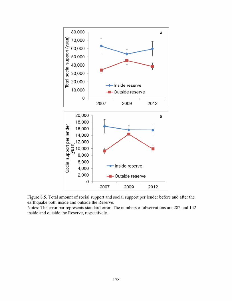
178
Figure 8.5. Total amount of social support and social support per lender before and after the earthquake both inside and outside the Reserve. Notes: The error bar represents standard error. The numbers of observations are 282 and 142 inside and outside the Reserve, respectively.
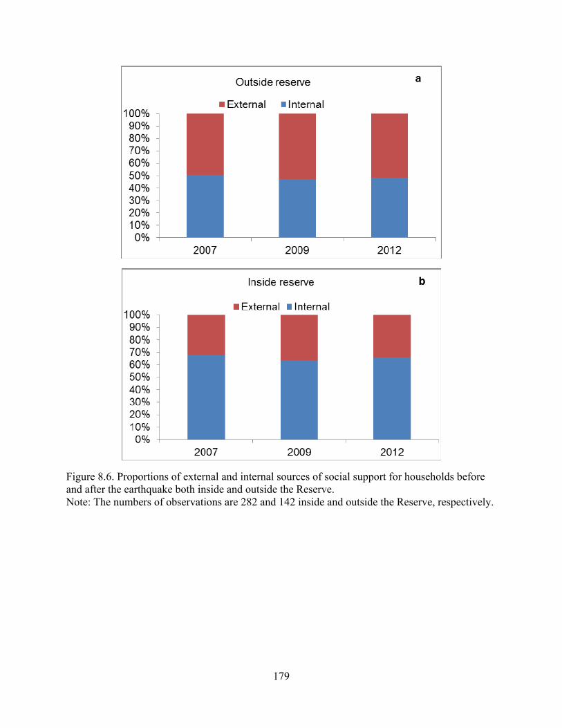
179
Figure 8.6. Proportions of external and internal sources of social support for households before and after the earthquake both inside and outside the Reserve. Note: The numbers of observations are 282 and 142 inside and outside the Reserve, respectively.

180
Figure 8.7. Dynamics of the gross household income inside and outside the Reserve from 1970s to 2010s. Notes: The numbers of observations are 169 and 157 inside and outside the Reserve, respectively. All monetary values were discounted into the constant values of 2010.

181
CHAPTER 9
CONCLUSIONS

182
The completion of this dissertation not only advances scientific understanding but also
provides information I hope will be useful for real-world management of human-nature
interactions in a variety of ways. Below I summarized the main advances in methodology and
scientific knowledge, and implications for decision making.
From a methodological perspective, the dissertation provided new methods to quantify
human dependence on ecosystem services (ES; Chapter 2), human well-being (HWB; Chapter 3),
and their linkages (Chapter 4). Using long-term datasets (e.g., survey data, satellite imagery,
field plots, government documents) and various models (e.g., Tobit model, spatial autoregressive
model, structural equation model), it offered strong evidence about the group-size effect that has
been debated for many decades (Chapter 5). Following Chapter 5, the multiple datasets and
mixed methods were also applied to address research questions in Chapters 6, 7 and 8. Such
integration of multiple datasets and mixed methods provide an excellent example illustrating
why and how to conduct interdisciplinary studies to address complex problems in Coupled
Human and Natural Systems (CHANS).
The quantitative and integrated approach to understand the linkages between ES and
HWB (Chapters 2, 3 and 4) suggests that the construction of quantitative indicators for ES and
HWB as well as integrated models is a viable approach for enhancing the understanding of
linkages between ES and HWB. The findings show that disadvantaged groups who possess low
levels of any form of capital except for natural capital are more dependent on ES than the
affluent that have greater control of capital. The findings also suggest that external drivers may
significantly affect both human dependence on ES and HWB with influence varies across
different components of ES or HWB. Those who are more vulnerable to disasters are
disadvantaged households with lower access to multiple forms of capital, more property damages,

183
or larger revenue reductions. Diversifying human dependence on ES helps to alleviate disaster
impacts on HWB. Since the approach is based on the generalizable Millennium Ecosystem
Assessment (MA) framework, it can be applied to different scales from local, regional to global
and different units of analysis (e.g., individual, household, enterprise, and nation).
The substantiation of nonlinear group size effects on collective action and resource
outcomes as well as the underlying mechanisms in Wolong Nature Reserve helps to guide future
research and governance of the commons (Chapter 5). The results show that intermediate group
size contributes the most to collective action and leads to the optimum resource management
outcomes. Such findings thus suggest that altering factors (e.g., punishing free riding, enhancing
enforcement, improving social capital, and allowing self-selection for group formation) that lead
to the nonlinear group-size effect can improve collective action and resource outcomes. The
findings also explain why previous studies have observed contradictory group-size effects by
focusing on a portion of the nonlinear curve and why a holistic approach should be taken to
address complex problems not only in common-pool resource management but also in all other
CHANS research.
Inspired by the findings, methods, and research process of the nonlinear group-size effect,
Chapter 6 examined different forms of hypothetical interaction effects of policies, which
generated some additional important findings. The results suggest that there are synergistic and
antagonistic effects among conservation and/or development policies, which can even lead to
unanticipated consequences. In our case, the payments from two conservation policies separately
had a negative effect on household income, but jointly led to a positive effect. Such findings
challenge the traditional realm of policy studies that often treat multiple policies separately and

184
again advocate a holistic approach by considering policy interactions, jointly designing,
monitoring, and evaluating policies.
Learned from previous chapters, Chapter 7 evaluated the effects of the Natural Forest
Conservation Program (NFCP) on both ES (using forest cover as an indicator) and HWB (using
income, indicators of energy use, and attitude metrics), with consideration of the interactions
between NFCP and other concurrent policies (e.g., Grain-to-Green Program, Tourism
Development Program, and Electricity Subsidy Program). The results suggest that NFCP had an
overall positive effect on ES, and mixed effects on local households’ well-being. Based on the
results, field observations, and local knowledge, the underlying mechanisms of the effects on ES
and HWB were discussed, which provide insights (e.g., integrating local conditions and
underlying mechanisms) for improving the design and implementation of policies not only in
Wolong Nature Reserve but also other places around the world.
Given the human-nature interactions, previous chapters have illustrated how complex the
effects and underlying mechanisms of policies on both ES and HWB could be. Chapter 8 further
confirmed this point and argued why and how scientific knowledge should be seriously taken
into policy design and implementation so as to achieve positive outcomes both for ES and HWB.
Chapter 4 confirmed that high access to natural, human, manufactured, and/or social capitals
before the earthquake had helped households to prevent or mitigate negative impacts. As a
further step, Chapter 8 evaluated how post-disaster reconstruction efforts affected the four forms
of capital, which often are assumed to be positive. Unfortunately, the results actually show the
opposite with an overall deteriorating trend of household capital after five years’ reconstruction,
despite two billion yuan (1 US dollar = 6.2 yuan as of July 2013) had been investing for
reconstruction. While the overall capital at the reserve level seems to be improving with the huge

185
amount of reconstruction investment, the findings suggest that the effects of post-disaster
reconstruction efforts can differ from one scale to another. Therefore, capacity building and
recovery should not be taken for granted and require integrated planning and implementation
targeting each form of capital at multiple scales.
It should also be noted that much of my work in this dissertation benefits from the long-
term effort to collect multiple kinds of data in WNR and surrounding areas. The lack of long-
term high quality data perhaps is the biggest problem in environmental science research and in
our ability to manage CHANS.
While this dissertation made a number of contributions to methodology and scientific
knowledge and provides a number of policy implications as mentioned above, it also opens the
door for further scientific inquiries. For instance, further research can apply our quantitative and
integrated approach in other studies both in Wolong Nature Reserve and other areas in China and
the rest of the world to test interesting hypotheses, answer important questions, and addressing
pressing problems for sustainability (see example hypotheses and questions in Table 4.2). Future
research can also follow our multiple datasets and mixed methods to investigate what contextual
factors determine the optimum group size either for the provision of collective action or resource
outcomes. The accumulated knowledge from a set of literature will hopefully lead to coherent
theories (e.g., human-nature feedbacks theory, vulnerability/resilience theory of CHANS) to
guide the management of human-nature interactions.

186
APPENDICES
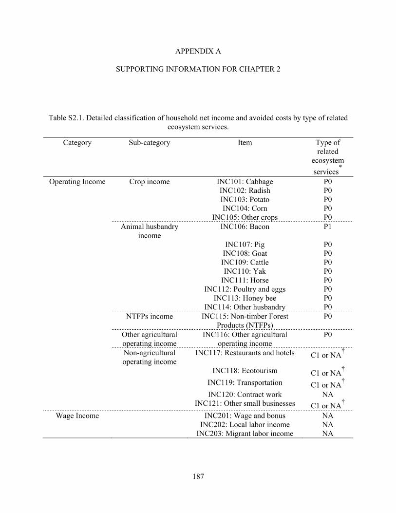
187
APPENDIX A
SUPPORTING INFORMATION FOR CHAPTER 2
Table S2.1. Detailed classification of household net income and avoided costs by type of related ecosystem services.
Category Sub-category Item Type of related
ecosystem
services*
Operating Income Crop income INC101: Cabbage P0 INC102: Radish P0 INC103: Potato P0 INC104: Corn P0 INC105: Other crops P0 Animal husbandry
income INC106: Bacon P1
INC107: Pig P0 INC108: Goat P0 INC109: Cattle P0 INC110: Yak P0 INC111: Horse P0 INC112: Poultry and eggs P0 INC113: Honey bee P0 INC114: Other husbandry P0 NTFPs income INC115: Non-timber Forest
Products (NTFPs) P0
Other agricultural operating income
INC116: Other agricultural operating income
P0
Non-agricultural operating income
INC117: Restaurants and hotels C1 or NA†
INC118: Ecotourism C1 or NA†
INC119: Transportation C1 or NA†
INC120: Contract work NA INC121: Other small businesses C1 or NA
†
Wage Income INC201: Wage and bonus NA INC202: Local labor income NA INC203: Migrant labor income NA
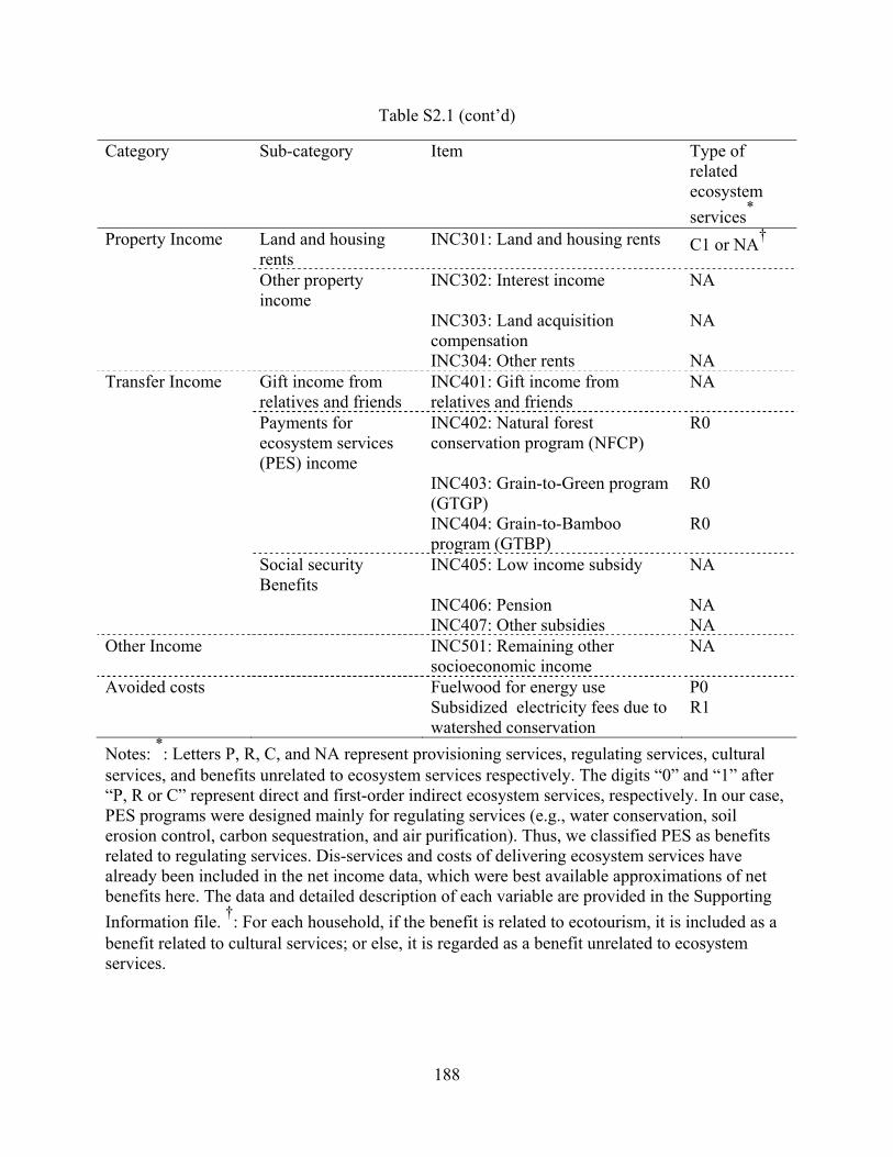
188
Table S2.1 (cont’d)
Category Sub-category Item Type of related ecosystem
services*
Property Income Land and housing rents
INC301: Land and housing rents C1 or NA†
Other property income
INC302: Interest income NA
INC303: Land acquisition compensation
NA
INC304: Other rents NA Transfer Income Gift income from
relatives and friends INC401: Gift income from relatives and friends
NA
Payments for ecosystem services (PES) income
INC402: Natural forest conservation program (NFCP)
R0
INC403: Grain-to-Green program (GTGP)
R0
INC404: Grain-to-Bamboo program (GTBP)
R0
Social security Benefits
INC405: Low income subsidy NA
INC406: Pension NA INC407: Other subsidies NA Other Income INC501: Remaining other
socioeconomic income NA
Avoided costs Fuelwood for energy use P0 Subsidized electricity fees due to
watershed conservation R1
Notes: *: Letters P, R, C, and NA represent provisioning services, regulating services, cultural
services, and benefits unrelated to ecosystem services respectively. The digits “0” and “1” after “P, R or C” represent direct and first-order indirect ecosystem services, respectively. In our case, PES programs were designed mainly for regulating services (e.g., water conservation, soil erosion control, carbon sequestration, and air purification). Thus, we classified PES as benefits related to regulating services. Dis-services and costs of delivering ecosystem services have already been included in the net income data, which were best available approximations of net benefits here. The data and detailed description of each variable are provided in the Supporting
Information file. †: For each household, if the benefit is related to ecotourism, it is included as a
benefit related to cultural services; or else, it is regarded as a benefit unrelated to ecosystem services.

189
APPENDIX B
SUPPORTING INFORMATION FOR CHAPTER 3
Table S3.1. The index system for assessing human well-being based on the Millennium Ecosystem Assessment conceptual framework.
Indicator layer Indicator code and content ri-t before earthquake
ri-t after earthquake
Affordability to necessary food
Q1.2: Your household can afford enough food with nutrition to keep alive and healthy
0.64 0.66
Affordability to basic facilities and services
Q1.3: Your household can afford to access basic facilities (e.g., television, washer) and services (e.g., transportation)
0.62 0.64
Satisfaction with housing condition
Q1.4: You are satisfied with your housing condition (including size and quality)
0.50 0.40
Overall satisfaction with access to basic goods and services
Q1.5: Overall, you are satisfied with your household’s basic goods and services (e.g., food, clothe, living conditions, transportation) for life
0.68 0.64
Life safety Q2.1: Your household’s life safety in daily life is secure
0.59 0.46
Property safety Q2.2: Your household’s property safety in daily life is secure
0.54 0.49
Local crime incidence
Q2.3: The local crime incidence (e.g., theft, robbery, murder, other violent incidents) is low
0.51 0.41
Access to government protection
Q2.4: The police and judicial system is always ready to help
0.40 0.38
Reliability of government protection
Q2.5: The police and judicial system can be trusted
0.38 0.33
Security for resource access
Q2.6: It is safe to access basic goods and services such as food, water, and medicine etc. for life
0.56 0.49
Overall satisfaction with security
Q2.7: Overall, you are satisfied with your household security (e.g., life and property)
0.66 0.59

190
Table S3.1. (Cont’d)
Indicator layer Indicator code and content ri-t before earthquake
ri-t after earthquake
Physical health Q3.1: You are satisfied with your household’s physical health (including illness and injury)?
0.67 0.66
Mental health Q3.2: You are satisfied with your household’s mental health (including stress, depression, and problems with emotions)?
0.66 0.68
Rest
Q3.3: How often your household members do not get enough rest or sleep? (Options: 1. Always; 2. Often; 3. Sometimes; 4. Seldom; 5. Never)
0.50 0.60
Energy for daily life
Q3.4: How often your household members are not healthy or do not have enough energy for everyday life? (Options: 1. Always; 2. Often; 3. Sometimes; 4. Seldom; 5. Never)
0.59 0.63
Emotion
Q3.5: How often do your household members have negative feelings such as blue mood, despair, anxiety, depression? (Options: 1. Always; 2. Often; 3. Sometimes; 4. Seldom; 5. Never)
0.55 0.61
Leisure activities
Q3.6: How often do your household members have the opportunity for leisure activities? (Options: 1. Never; 2. Seldom; 3. Sometimes; 4. Often; 5. Always)
0.45 0.52
Overall satisfaction with health status
Q3.7: Overall, you are satisfied with your household’s health status
0.66 0.70
Close neighborhood
Q4.1: This is a close-knit neighborhood 0.53 0.43
Opportunities of neighborhood interactions
Q4.3: There are many opportunities to meet neighbors and work on solving community problems
0.31 0.37
Cohesion
Q4.6: Suppose someone in your village/neighborhood had something unfortunate happen to them, such as a family member's sudden death, there are always some others would be ready to help
0.37 0.39
Overall satisfaction with social relationship
Q4.7: Overall, you are satisfied with your household’s social relationships with others
0.38 0.36
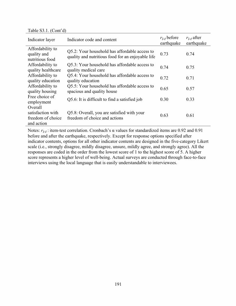
191
Table S3.1. (Cont’d)
Indicator layer Indicator code and content ri-t before earthquake
ri-t after earthquake
Affordability to quality and nutritious food
Q5.2: Your household has affordable access to quality and nutritious food for an enjoyable life
0.73 0.74
Affordability to quality healthcare
Q5.3: Your household has affordable access to quality medical care
0.74 0.75
Affordability to quality education
Q5.4: Your household has affordable access to quality education
0.72 0.71
Affordability to quality housing
Q5.5: Your household has affordable access to spacious and quality house
0.65 0.57
Free choice of employment
Q5.6: It is difficult to find a satisfied job 0.30 0.33
Overall satisfaction with freedom of choice and action
Q5.8: Overall, you are satisfied with your freedom of choice and actions
0.63 0.61
Notes: ri-t : item-test correlation. Cronbach’s α values for standardized items are 0.92 and 0.91 before and after the earthquake, respectively. Except for response options specified after indicator contents, options for all other indicator contents are designed in the five-category Likert scale (i.e., strongly disagree, mildly disagree, unsure, mildly agree, and strongly agree). All the responses are coded in the order from the lowest score of 1 to the highest score of 5. A higher score represents a higher level of well-being. Actual surveys are conducted through face-to-face interviews using the local language that is easily understandable to interviewees.

192
Table S3.2. Standardized coefficients of the confirmatory factor analysis for Human Well-Being Index (HWBI).
Dependent variable Independent variable
Standardized coefficients
Robust S.E.
Overall HWBI Q1 0.613***
0.034
Q2 0.662***
0.045
Q3 0.914***
0.042
Q4 0.638***
0.054
Q5 0.584***
0.034
Q1:Basic material for good life
Q1.2 0.826***
0.018
Q1.3 0.829***
0.018
Q1.4 0.235***
0.043
Q1.5 0.427***
0.035
Q3.6 0.218***
0.044
Q5.2 0.657***
0.080
Q5.3 0.374***
0.079
Q2:Security Q2.1 0.617***
0.035
Q2.2 0.602***
0.035
Q2.4 0.336***
0.042
Q2.5 0.314***
0.042
Q2.6 0.381***
0.044
Q2.7 0.818***
0.027
Q1.4 0.262***
0.044
Q1.5 0.368***
0.040
Q3.2 0.199***
0.046
Q3:Health Q3.1 0.787***
0.026
Q3.2 0.642***
0.042
Q3.3 0.618***
0.033
Q3.4 0.700***
0.027
Q3.5 0.597***
0.032
Q3.7 0.826***
0.021

193
Table S3.2. (Cont’d)
Dependent variable Independent variable
Standardized coefficients
Robust S.E.
Q4:Good social relations Q4.1 0.548***
0.039
Q4.3 0.300***
0.041
Q4.6 0.438***
0.037
Q4.7 0.417***
0.043
Q2.3 0.533***
0.035
Q3.6 0.367***
0.048
Q5:Freedom of choice and action
Q5.2 0.263***
0.075
Q5.3 0.553***
0.080
Q5.4 0.909***
0.017
Q5.5 0.784***
0.024
Q5.6 0.274***
0.041
Q5.8 0.808***
0.023
Q2.6 0.226***
0.043
Q1 Q5 0.738***
0.033
Q2 Q4 0.686***
0.075
Notes: ***
p < 0.001. For description of each code, please refer to Appendix A. Only paths that are theoretically meaningful are added. Only paths with coefficients that are tested to be significant (p < 0.05) are included in the model. Paths between observed indicators are not shown here. The confirmatory factor analysis is constructed using the MLR estimator in Mplus. The number of total observations is 326.

194
APPENDIX C
SUPPORTING INFORMATION FOR CHAPTER 4
Table S4.1. Descriptive statistics of variables used in the model. Variable Mean (S.D.) Change of HWBI – 0.080 (0.010) HWBI in 2007 0.638 (0.118) IDES in 2007 0.634 (0.295) Change of IDES – 0.303 (0.423) Non-agricultural income share in 2007 0.581 (0.283) Household income in 2007 (thousand yuan) 28.651 (304.954) Household income in 2009 (thousand yuan) 68.105 (104.715) Change of household income per capita (thousand yuan)
11.160 (35.306)
Household size in 2007 3.317 (1.319) Number of seniors (age >= 60 years) 0.653 (0.805) Average education of adults in 2007 (year) 5.052 (2.760) Female adult share in 2007 0.469 (0.165) House damage (0: low, 1: high) 0.624 (0.487) Social ties to local leaders (0: weak, 1: strong) 0.109 (0.313) Gender of interviewee (0: female, 1: male) 0.584 (0.495) Age of interviewee (year) 53.604 (11.333) Notes: Change of HWBI, change of IDES, or change of household income per capita are calculated as the corresponding values in 2009 subtracting the corresponding values in 2007, respectively. A household with strong social ties to local leaders is defined as a household with at least one household member or one immediate relative (e.g., parents, children, and blood brothers) as local leaders; otherwise it is defined as one with weak social ties to local leaders. The number of observations is 101.

195
Table S4.2. Impacts of the earthquake on net benefits from socioeconomic activities and ecosystem services. Overall index/sub-index Before earthquake
(2007) After earthquake (2009)
t value
Net socioeconomic benefit (thousand yuan)
13.899 (2.612) 57.681 (9.964) – 4.434***
Net benefit from provisioning services (thousand yuan)
10.279 (1.842) 3.063 (0.959) 4.821***
Net benefit from regulating services (thousand yuan)
3.519 (0.226) 3.468 (0.250) – 0.730
Net benefit from cultural services (thousand yuan)
0.992 (0.390) 0.424 (0.251) 1.686*
Notes: Numbers outside and inside parentheses are means and standard errors, respectively. Monetary values for net benefits in 2009 were discounted into present values of 2007 for
comparison. The sampled households in 2007 and 2009 are the same 101 households. *p < 0.05,
***p < 0.001.

196
Table S4.3. Associations between HWBI and affluence before and after the earthquake.
HWBI in 2007 before earthquake
HWBI in 2009 after earthquake
Household income in 2007 (yuan) 0.309
** 0.291
**
Household income in 2009 (yuan) 0.254
* 0.309
**
Notes: Numbers are Spearman’s rho. The number of observations is 101. *p < 0.05,
**p < 0.01.

197
Table S4.4. Supplementary regressions for factors associated with the change of HWBI before and after the earthquake. Dependent variable: Change of HWBI Model (1) Model (2) Model (3) HWBI in 2007 – 0.116 (0.082) – 0.119 (0.082) – 0.117 (0.081) Net benefit from provisioning services in 2007 (thousand yuan)
2.13e-04 (5.29e-04)
– –
Net benefit from regulating services in 2007 (thousand yuan)
– – 0.003 (0.005) –
Net benefit from cultural services in 2007 (thousand yuan)
– – 0.001 (0.002)
Change of IDES – 0.033 (0.029) – 0.027 (0.027) – 0.030 (0.028) Agricultural income share in 2007 – 0.065 (0.052) – 0.064 (0.044) – 0.053 (0.044) Household income in 2009 (thousand yuan)
3.27e-04*
(1.50e-04) 3.48e-04
*
(1.33e-04) 3.36e-04
*
(1.41e-04) Change of per capita income (thousand yuan)
– 8.38e-04 (5.42e-04)
– 9.38e-04*
(4.28e-04) – 8.94e-04
*
(4.35e-04) Household size in 2007 0.012
* (0.006) 0.014
* (0.006) 0.012
* (0.006)
Number of seniors (age >= 60 years) – 0.021 (0.017) – 0.023 (0.017) – 0.022 (0.017) Average education of adults in 2007 (year)
0.006 (0.004) 0.006 (0.005) 0.006 (0.005)
Female adult share in 2007 – 0.090 (0.071) – 0.087 (0.070) – 0.094 (0.072) House damage (0: low, 1: high) – 0.043
*
(0.018) – 0.041
*
(0.018) – 0.044
*
(0.018) Social ties to local leaders (0: weak, 1: strong)
0.040 (0.025) 0.038 (0.026) 0.040 (0.026)
Gender of interviewee (0: female, 1: male)
0.033 (0.019) 0.032 (0.019) 0.033 (0.019)
Age of interviewee (year) 1.60e-05 (0.001)
5.36e-05 (0.001)
6.39e-05 (0.001)
Constant – 0.018 (0.077) – 0.008 (0.081) – 0.018 (0.077) F-statistic 2.01
* 2.13
* 2.08
*
R-squared 0.2485 0.2514 0.2490 N 101 101 101 Notes: Dependent variable is the change of HWBI before and after the earthquake, which is HWBI in 2009 subtracting HWBI in 2007. Numbers inside and outside parentheses are
coefficients and robust standard errors, respectively. *p < 0.05. Variance inflation factors are
tested to be less than 5.

198
APPENDIX D
SUPPORTING INFORMATION FOR CHAPTER 5
1. Supporting methods
1.1. Data
1.1.1. Remotely sensed and geographic information system data
We acquired a map and associated documentation (e.g., the number of households for
monitoring each forest parcel) of the Natural Forest Conservation Program (NFCP) monitored
parcels from the administrative bureau of Wolong Nature Reserve (WNR). Of ~40,100 ha in
household monitoring areas, ~24,300 ha in 152 parcels involving 812 households had explicit
household monitoring boundaries delineated on the map. Of these 152 parcels, 23 were
monitored by single households. The remaining ~15,800 ha have boundaries described in the
documentation but not on the map. These non-mapped areas were all monitored by single
households. We verified that even excluding the 23 parcels, the nonlinear group-size effect on
forest outcomes (Table 5.2) still holds (see details in Section 2.5.2). In addition, one parcel co-
monitored by nine households and located on the boundary between WNR and the adjacent
Sanjiang Township is known to experience intensive land conversion due to tourism
development. A Bonferonni test for most extreme observations (Fox, 1997) also indicates this
parcel is the only outlier in our dataset (for this parcel, studentized residuals = – 3.786,
Bonferonni p-value < 0.05; all other parcels had Bonferonni p-value > 0.05). Therefore, we
excluded this parcel and used the remaining 151 spatially explicit parcels (Fig. 5.2) for our study.
We used previously published forest-cover maps derived from Landsat imagery in 2001
and 2007 to estimate forest-cover change (Viña et al., 2007; Viña et al., 2011). We generated

199
forest-cover maps via an unsupervised classification algorithm using the ISODATA technique,
an iterative process for non-hierarchical pixel classification (Jensen, 1996). We performed
accuracy assessments using ground-truth points obtained in the summers of 1998 (209 points),
2000 (83 points), 2001 (83 points), and 2007 (593 points). We measured these points using GPS
receivers with high accuracy (error less than 1 m). Overall accuracies of these maps were
between 80% and 83%. Major disagreements occurred primarily in high-elevation areas and with
complex topography (i.e., northwestern part of WNR, Fig. 5.2) rather than in the areas monitored
by households that are the focus of our study. Thus, classification accuracies of the selected
household monitoring areas should be higher than those of the overall maps. In addition, changes
in land cover between field and remotely sensed data collection dates partially accounted for the
disagreement between the image classification and ground-truth data. For a detailed description
of classification procedures and assessments of map accuracy, please refer to the citied studies
(Viña et al., 2007; Viña et al., 2011).
We obtained data on topographic characteristics such as elevation, slope, and the
Compound Topographic Index, a relative measure of wetness (Gessler et al., 1995), from a
digital elevation model at a spatial resolution of 90 m/pixel, acquired by the Shuttle Radar
Topography Mission (Berry et al., 2007). We measured all household locations inside and
surrounding WNR using GPS receivers. Based on the digitized NFCP parcel map and forest-
cover maps, we calculated the size of each parcel, parcel size per household, average elevation,
average slope, average wetness, distance between each parcel and the nearest household,
distance between each parcel and the main road, distance between each household and its
monitored parcel, distance between each household and the main road, initial forest cover in
2001, and the percent of forest cover change from 2001 to 2007.

200
1.1.2. Focus group, personal, and household interviews
Our research team has been investigating our study area since 1995, starting six years
before the NFCP implementation. We drew upon both our experience in the area and the best
available data collected by our research team in studying the underlying mechanisms of
nonlinear group-size effects, supplementing quantitative analysis with information obtained from
qualitative interviews.
We conducted focus group and personal interviews on NFCP in 2007. For retrospective
information, we used the standard practice of life-history calendars to enhance respondents’
recall accuracy (Axinn et al., 1999; Freeman et al., 1988). These interviews were collected to
understand the NFCP planning, implementation, evaluation, and decision-making processes and
to prepare for the household interview. For focus group interviews, we interviewed eight
members of the WNR administrative staff. For personal interviews, we held discussions with
five officials who were and/or are in charge of the NFCP planning, implementation, evaluation,
and decision making. Our understanding of how the monitoring groups were formed was based
on focus groups and personal interviews, and we further examined the criteria of group
assignment with household survey data (see Section 1.2).
From household interviews, we used data acquired from all households that participated
in the NFCP in 2007 (surveyed at the end of 2007) and 2009 (surveyed in the summer of 2010).
Usually the household heads or their spouses were chosen as interviewees because they are the
decision makers and are familiar with household affairs. We tracked the same randomly sampled
households across the years, but some households were missing in one year or another. For
instance, some households were merged, some naturally died out, and some were away for
201
migrant work during our entire investigation period in a given year. A total of 156 NFCP
households covering the full range of group size (i.e., from 1 to 16) were interviewed in 2007 to
examine how group size affects collective action (i.e., household forest monitoring), and 113
households for group size larger than one were interviewed in 2009 to examine the mechanisms
of nonlinear group-size effects. For each analysis, to avoid errors due to using data from different
survey years, we only used factors that were measured for all households in the same year. The
information elicited included demographic factors, household socioeconomic activities, social
ties to local leaders, NFCP payment received, NFCP monitoring effort, and within-group
monitoring enforcement. The instrument for household socioeconomic data was based on the
standard practices of the National Bureau of Statistics of China (National Bureau of Statistics of
China, 2011). Please see a detailed description of variables used for analyses in Section 2.
1.2. Study area and group formation
Wolong Nature Reserve (N 30˚45' – 31˚25', E 102˚52' – 103˚24') is located in Wenchuan
County, Sichuan Province, China (Fig. 5.2). It is situated in the transition of Sichuan Basin from
the east to the Qinghai-Tibet Plateau on the west, with elevations ranging from 1,200 m to 6,250
m. WNR’s size was ~20,000 ha in 1963 and expanded to its current size of ~200,000 ha in 1975
(Wolong Nature Reserve, 2005). The Reserve was established to protect regional forest
ecosystems and rare plant and animal species, primarily the iconic giant panda (Ailuropoda
melanoleuca) (Wolong Nature Reserve, 2005). The majority of local residents are farmers
involved in activities such as cultivating maize and vegetables, raising livestock (e.g., pigs, cattle,
yaks, horses), collecting traditional Chinese medicinal plants, beekeeping, and collecting

202
fuelwood for heating and cooking. Basic demographic and socioeconomic descriptions are
summarized with our household survey data in Table S5.1.
NFCP is a nationwide conservation program that aims to conserve and restore natural
forests with logging bans, afforestation, and monitoring using a payments-for-ecosystem-
services scheme to motivate conservation behavior (Liu et al., 2008). To respond to the national
call, and to restrain the degradation of forest and panda habitat over the past three decades (Liu et
al., 2001), WNR started to implement the NFCP in 2001. The central government allocated an
annual fund of two million yuan for NFCP implementation in the Reserve. To improve
enforcement of the NFCP and livelihoods of local residents, the Wolong Administrative Bureau
decided to use about half of the NFCP funds to engage local households in the forest monitoring
program (Wolong Nature Reserve, 2005).
The initial idea of the Wolong Administrative Bureau was to assign each household a
forest parcel to monitor, but it turned out to be too difficult to clarify the boundaries of many
small parcels and would be too costly for management. Finally, the Bureau followed natural
boundaries (e.g., rivers, ridges, valleys) of forest parcels and divided and assigned them to
household groups ranging from 1 to 16. Of the total ~120,500 ha NFCP monitoring area,
~40,100 ha were assigned to ~1,100 rural households; the remaining areas were monitored
directly by the Bureau’s staff (Fig. 5.2).
According to our interviews with government officials who were in charge of the NFCP
implementation, large parcels were assigned to large household groups to keep parcel size per
household similar across monitoring areas. Parcels distant from household locations were
assigned to large household groups with slightly higher payments. We compared these
arrangements with our independently collected household survey data and found the reports from

203
household interviewees were consistent with those from the program officials (Table S5.2). We
also conducted statistical analyses and found that the distance from each parcel to its monitoring
household(s) and NFCP payment were statistically exogenous to the group-size effects (see
Section 2.4.3). Thus, distribution of households to groups, although not completely random as in
a classical experiment, is suitable to examine the group-size effects and the underlying
mechanisms.
1.3. Tobit model
1.3.1. Model specification
The dependent variable is the total labor input per year by a household for monitoring.
The distribution of this variable suggests a Tobit model, in which a large fraction of the
observations cluster at the minimum value (zero in this case) or maximum value (20 in this case).
Conceptually, this is a censored value model in that it treats the minimum and maximum values
as if the values of monitoring were not observed. The minimum monitoring effort is zero by
default, which means a household does not spend any time in monitoring. According to our field
investigation, the maximum annual payment for monitoring is ~1,000 yuan, and the local labor
price in 2007 was ~50 yuan per laborer per day. This suggests the maximum monitoring effort of
a household is 20 laborer days if they are strict economic humans. This theoretical estimate was
consistent with empirical data collected from reports of local natural resource managers and
monitoring households. In other words, households spent an amount of labor less or equal to
what they received in NFCP payments. Thus, besides zero as the minimum monitoring effort, we
also set 20 as the maximum value in the Tobit model.

204
When analyzing censored data, traditional regression methods (e.g., ordinary least
squares, OLS) may yield inconsistent estimates and provide inappropriate predictions. However
censored regression (i.e., Tobit model) can produce consistent and efficient estimates of model
parameters and partial effects, as well as appropriate predictions (Wooldridge, 2002). A Tobit
model is given by (Wooldridge, 2002):
biyb
aiya
biyaiy
iy*1
*1
*1
*1
1 (5.1)
iuiXiy 11*1 , (5.2)
where iy1 is the observed monitoring effort, *1iy is a latent variable satisfying the classic linear
model assumption, a is the minimum limit, b is the maximum limit, iX1 is a vector of
exogenous explanatory variables, 1 is a parameter vector to be estimated, i is the ith observation,
and iu is an error term that has a normal distribution with mean of zero.
When the Tobit model contains endogenous variables, Eq. (5.2) is specified as follows
(Wooldridge, 2002):
iuiXiyiy 1122*1 (5.3)
iviXiXiy 22112 , (5.4)
where iy2 is a vector of potentially endogenous explanatory variables and the equation for iy2
is written in reduced form, iX1 is a vector of exogenous explanatory variables, iX2 is a vector
of additional instruments, 2 is a vector of structural parameter, 1 and 2 are matrices of

205
reduced-form parameters, and iv is an error term that has a normal distribution with mean of
zero.
1.3.2. Model construction
Descriptive statistics of variables used in model construction are shown in Table S5.1. To
improve the interpretability of coefficients and reduce the collinearity between the linear and
quadratic terms of group size, all continuous independent variables and instruments were mean
centered prior to their input into the regression models (Schielzeth, 2010). We first constructed
our models with OLS without considering the censoring effects, then constructed the Tobit
models considering the censoring effects. Whether or not we took the censoring effects into
account, the nonlinear group-size effects were consistent. Thus, we reported the final results
from the Tobit models. Parameter and marginal effect estimations were conducted using Stata 12
(StataCorp LP, USA).
1.4. Spatial autoregressive model
1.4.1. Model specification
Previous studies on group-size effects have not considered the spatial autocorrelation of
measurements across resource units (e.g., forest parcels) of key variables (e.g., percent of forest-
cover change). Ignoring spatial autocorrelation may violate the assumption of independently
distributed errors of classical statistical tests and may lead to incorrect conclusions (Lichstein et
al., 2002). In brief, the ecological reason for considering spatial autocorrelation here is that a
parcel is more likely to regenerate or recover faster when its surrounding parcels are forested

206
(Lichstein et al., 2002). We constructed spatial autoregressive models to take spatial
autocorrelation into consideration.
The general mixed form of the spatial autoregressive model in our study is given by
(Anselin, 1988; LeSage and Pace, 2009):
y = ρWy + Xβ + μ (5.5)
μ = λWμ + ε, (5.6)
where y is the n (number of observations) × 1 vector of the dependent variable (i.e., percent of
forest-cover change from 2001 to 2007), ρ is the coefficient of the spatially lagged dependent
variable, W is a given n × n spatial weighting matrix, X is the n × k (number of independent
variables plus intercept) matrix of the independent variables plus intercept, β is the k × 1 vector
of coefficients, λ is the spatial error correlation coefficient, and ε is the n × 1 error term assumed
to be independent and identically distributed. The mixed model is reduced to a spatial lag model
when λ = 0, to a spatial error model when ρ = 0, and to a traditional regression model when both
are zero.
1.4.2. Model construction
Descriptive statistics of variables used in the model construction are shown in Table S5.3.
A spatial weighting matrix of forest parcels was created using the GeoDa software (version
0.9.9.1), defining a neighbor based on the Queen contiguity approach (i.e., common borders and
corners) (Anselin et al., 2006). We compared different spatial weighting matrices (i.e., Queen
contiguity of order 1, Queen contiguity of order 2, Rook contiguity of order 1, and Rook
contiguity of order 2), and the results are similar. Thus, we reported the results using Queen
contiguity of order 1. Model construction and all statistical analyses were performed using the R

207
software (version 2.12.2) (R Development Core Team, 2011). Spatial simultaneous
autoregressive models were constructed with the package “spdep” in R.
1.5. Structural equation model
1.5.1. Model specification
A structural equation model (SEM) is a statistical technique for testing and estimating
causal relationships (Pearl, 2000; Simon, 1953; Wright, 1921). It allows analysis of multiple
simultaneous causal relations among endogenous variables, and between endogenous and
exogenous variables. A typical SEM contains two main components: the structural model
representing potential causal dependencies between endogenous and exogenous variables, and
the measurement model representing the relations between latent variables and their indicators.
The general form of SEM is given by (Bollen and Noble, 2011):
Structural model:
jjjBj (5.7)
Measurement model:
jjyyjy (5.8)
jjxxjX , (5.9)
where j is the vector of latent endogenous variables for unit j; , y , and x are intercept
vectors; j is the vector of latent exogenous variables; jy and jX are vectors of the observed
indicators of j and j , respectively; B is the matrix of coefficients giving the expected effects
of the latent endogenous variable ( ) on each other; Γ is the coefficient matrix giving the
expected effects of the latent exogenous variables (ξ) on the latent endogenous variables ( );

208
y and x are the matrices of coefficients giving the effects of the latent j and j on jy
and jX , respectively; j , j , and j are the vectors of error terms; and j is the jth observation.
The commonly used factor analysis, regression analysis, and path analysis methods are
all special cases of SEM. Specifically, path analysis is SEM with a structural model but no
measurement model. In this study, all variables can be reasonably treated as observable. So we
used SEM for path analysis of the nonlinear group-size effects. Guided by the two hypothetical,
opposing forces through which group size affects collective action and then resource outcomes,
based on previous literature, we hypothesized that some factors may affect group size, group size
may directly affect free riding, and group size may also indirectly affect free riding through
within-group enforcement (Fig. 5.1).
1.5.2. Model construction
Descriptive statistics of variables used in the model are shown in Table S5.4. Three
structural models of increasing complexity were constructed. First, whether or not a household
would be a free rider was estimated as a function of the size of its group and within-group
enforcement. Second, within-group enforcement was estimated as a function of monitoring
group size, whether or not there was within-group division (see description in Section 2.3), and
interaction term of group size and within-group division. Third, other factors that may affect
group size were controlled as exogenous variables acting on group size. Because some dependent
variables are binary (i.e., free rider and within-group enforcement), we conducted the path
analysis using Mplus (Muthén and Muthén, 1998-2010), which handles path analysis with
categorical outcomes. We used the default robust weighted least squares (WLSMV) estimator,
which uses a diagonal weight matrix with standard errors adjusted, and mean- and variance-

209
adjusted chi-square test statistics (Muthén and Muthén, 1998-2010). The final path model
retained some variables that were not significant because the goodness of fit of the path model
was high (Table S5.5), and because those variables were theoretically interesting as controls (see
Section 2.3).
2. Supporting text and analysis
2.1. Forest monitoring and within-group enforcement
2.1.1. Monitoring efforts: household labor input
The forest monitoring efforts of each household were measured by the total amount of
labor input. One unit of labor input was defined as one work day (i.e., eight work hours) of a
laborer spent on monitoring activities, including the time travelling to and from the monitored
parcel. In our data, each household either does not send any laborer or sends only one laborer for
each monitoring activity to join with other laborers from the assigned monitoring group.
Therefore, for each household, the total annual amount of labor input equals the total work days
that one laborer spent on monitoring (Eq. 5.10).
Household labor input (laborer days) = Monitoring frequency (times) × Time per monitoring
(hours) / 8 (hours day-1
laborer-1
) (5.10)
Illegal logging activities can be detected in several ways. First, because many households
live near the forest and conduct agricultural activities in and around the forest, they can hear the
sounds of cutting and falling trees. Local households can also see illegal loggers when they
transport the timber to their homes or along the main road to outside areas (because it is a
mountainous area with complex topography, it is very difficult to transport wood except via the
main road). Second, for forests far from local households, illegal activities may be detected by
210
households who are monitoring the forests or other people who happen to pass by as they collect
fulewood or conduct other legal activities. Local households are motivated to report illegal
activities because the local government rewards reporters in cash. Finally, even if these ways fail,
the timber checkpoints at the two ends of the main road across the reserve also can detect
illegally logged timber.
2.1.2. Free riders
Free riders are defined as people who receive the NFCP payment but do not spend time
and labor on forest monitoring. Here, we classified those households who self-reported that they
did not conduct monitoring activities as free riders. Our team has been conducting research in
this study area since 1995 and has established good social relationships with local households.
Social desirability would incline respondents toward overreporting their monitoring efforts. Thus,
we could be reasonably certain that those households reporting zero monitoring effort did in fact
free ride.
2.2. Forest monitoring outcomes: changes in forest cover
The main aim of assigning forest parcels to households for monitoring is to prevent
logging. Thus, to assess the outcomes of household monitoring efforts, the most important
indicator is the number of trees in each parcel. However, it is difficult and costly, if not
impossible, to count all trees. An alternative approach is to assess the forest cover. We adopted
the forest definition of the Food and Agriculture Organization of the United Nations as “Land
spanning more than 0.5 hectares with trees higher than five meters and a canopy cover of more
than 10 percent, or trees able to reach these thresholds in situ” (Forestry Department of Food and
211
Agriculture Organization of the United Nations, 2010). Detailed descriptions of the forest-cover
data are summarized in Section 1.1 and our previous publications (Viña et al., 2007; Viña et al.,
2011). The forest monitoring outcome was therefore measured on a per-parcel basis by percent
forest-cover change (i.e., percent forest cover in 2007 minus percent forest cover in 2001).
2.3. Structural factors
Two main barriers for examining group-size effects are the heterogeneities of groups and
resource units (Gautam, 2007; Ostrom, 1990; Poteete and Ostrom, 2004). In this section, we
provide a review of structural factors used in our analyses. We include factors commonly found
to be relevant to collective action and commons management (Agrawal and Goyal, 2001; Baland
and Platteau, 1996; Ostrom, 1990; Rustagi et al., 2010): characteristics of household groups,
households, and forest parcels.
2.3.1. Characteristics of household groups
Group size. Group size refers to the number of households for monitoring a single forest parcel.
Within-group enforcement. We regarded a group as having strong monitoring enforcement if
punishment measures (e.g., payment deduction, verbal condemnation) existed within the group
for members who did not participate in monitoring (i.e., free riding). Otherwise, we regarded a
group as having weak monitoring enforcement.
Within-group division. Groups with two or more households could divide laborers to improve
monitoring efficiency. In our case, if groups were divided into small subgroups to conduct
monitoring in turns, we coded them as groups having within-group division of labor; otherwise,
groups did not have within-group division of labor.

212
2.3.2. Characteristics of households
Household size. Household size refers to the number of household members.
Education of adults. Education affects an individual’s attitude and behavior (Rustagi et al.,
2010). Since adult household members are the main decision makers of household activities and
actually participate in forest monitoring, we used the average education level of all adult
household members.
Number of laborers. The number of laborers in a household is a measure of available household
labor resources for the forest monitoring activity. A laborer is defined as an individual between
the ages of 15 and 59.
Social ties to local leaders. Social organization in rural areas in China (such as our study area) is
largely based on kinship and leadership. Local leaders are well documented to be influential on
the behavior of group members (Rustagi et al., 2010). Therefore, we expected connections to
local leaders to affect a household’s contribution to collective action. In our study area,
individuals who work as leaders in villages, administrative groups, or local government-owned
enterprises are widely regarded as local leaders. We defined a household with strong social ties
to local leaders as a household that had at least one household member or one immediate relative
(e.g., parent, child, brother) who was a local leader; otherwise, a household had weak social ties
to local leaders.
Age of adults. As individuals get older, their household structures and social ties also change
because their relatives and friends die, and/or their children leave home. Thus, the age structure
of a household may be an important factor affecting social ties to local leaders. Since adult

213
household members are the actors for social ties connecting to local leaders, we used the average
age of all adult members of a household as the age structure measurement for each household.
Percentage of adult females. Gender plays an important role in developing different social ties
(van Emmerik, 2006). Thus, differences in the proportion of women among adult household
members may contribute to the differences in households’ social ties to local leaders. The
percentage of adult females among adults refers to the ratio of the number of female adults to
total adults in a household.
Household income. We acquired gross household income data from face-to-face interviews
following the standard protocol of the National Bureau of Statistics of China (National Bureau of
Statistics of China, 2011). In our study area, household income covers a wide range of categories
such as agricultural income (e.g., from animal husbandry, sales of crops and/or nontimber forest
products), wage income, small businesses income (e.g., operating restaurants, hotels, and other
tourism-based businesses), property income (e.g., land and housing rents), gift income from
relatives and friends, government payments for ecosystem services, and social security benefits
(e.g., low-income subsidy, pension).
Per capita household income. Per capita household income is the total household income
divided by household size.
Agricultural income. Agricultural income refers to income related to agricultural practices such
as cultivating cropland, raising livestock, and collecting nontimber forest products.
Percentage of agricultural income. The percentage of agricultural income is the ratio of
household agricultural income to its total household income.
Area of cropland. The area of cropland refers to the total area of cropland owned by a
household.

214
NFCP payment. NFCP payment refers to the amount of cash subsidy a household received for
participating in the NFCP forest monitoring program.
Distance between each household and the main road. In our study area, households farther
from the main road are likely to cultivate more cropland (Spearman’s ρ = 0.436, p < 0.001), rely
more on agricultural income (Spearman’s ρ = 0.249, p < 0.01), and are closer to their monitored
parcels (Spearman’s ρ = – 0.201, p < 0.05). Such reflected heterogeneity of households may also
affect their participation and contribution to forest monitoring.
Distance between each household and its monitored parcel. The further a household is away
from its monitored parcel, the longer distance the household must travel and the more time it
takes for a single monitoring activity. Therefore, the distance from each household to its
monitored parcel is a surrogate measure of monitoring cost. Because this factor was correlated
with group size and might cause an endogeneity problem (Table S5.2), we did not directly
include it in the models (Table 5.1 and 5.2). Instead, we treated it as a hypothesized instrumental
variable and examined whether the nonlinear group-size effects were caused by this factor or
indeed by the group size (see Section 2.4.3).
2.3.3. Characteristics of forest parcels
Elevation. Because elevation is correlated to climatic factors such as temperature, it is an
important factor influencing forest growth. Furthermore, elevation is also a natural barrier that
reduces human access. However, since household-monitored parcels are mainly located along
the main road and at relatively lower elevations, the variation of average elevation for each
parcel is not large (Table S5.3).

215
Slope. Similar to elevation, steeper slope reduces human access and thus reduces logging and
forest degradation.
Wetness. Wetness, as measured by the Compound Topographic Index, is a measurement of
relative soil moisture (Gessler et al., 1995). Soil moisture is an important factor affecting forest
growth (Viña et al., 2011). We expected forests to recover faster in relatively wetter regions.
Parcel size. Larger parcels are more exposed to logging and require more monitoring efforts to
prevent illegal access (Agrawal and Goyal, 2001). Therefore, the parcel size is an important
factor that may affect forest-cover changes.
Parcel size per household. Parcel size per household is the total size of a parcel divided by the
number of households assigned to monitor the parcel.
Initial forest cover in 2001. Initial forest cover is a key factor to determine the potential of
forest growth. A region with high initial forest cover does not have much room to grow and thus
forest regeneration is more likely to occur in places with relatively lower initial forest cover.
Distance between each parcel and the main road. Since most households and household-
monitored parcels are located along the main road (Fig. 5.2), illegal harvests closer to the main
road should be easier to catch. Therefore, the distance between each parcel and the main road is a
measurement of the difficulty of detecting illegal harvest. We used the distance from the centroid
of each parcel to the main road as an average estimate of distance for each parcel. The same
approximation of using the centroid of each parcel was adopted for measuring distances between
each parcel and other locations (e.g., the nearest household, each parcel’s corresponding
monitoring households).
Distance between each parcel and the nearest household. Distance between each parcel and
the nearest household is a factor measuring resource vulnerability to illegal harvest. Since

216
households tend to collect forest products (e.g., fuelwood) closer to their households, forests
closer to households may be more likely to suffer from illegal harvest.
2.4. Causality
Experiments with randomization are usually considered the best method for establishing
causal relationships. But such experiments are hard to conduct in the field and around policy
implementation, and laboratory experiments often suffer from a lack of external validity.
However, our 17-year investigation in our study area both before and after NFCP
implementation and evidence from the literature and supplemental analyses of our data suggest
that we have established plausible evidence for causal effects of group size on both collective
action (i.e., forest monitoring by household groups in our case) and resource outcomes (i.e.,
changes in forest cover in our case).
2.4.1. Why does collective action contribute to resource outcomes?
Evidence from literature. The “externality” characteristic of common-pool resources explains
why collective action could lead to their destruction (i.e., the tragedy of the commons) (Hardin,
1968). This conventional wisdom was challenged by the landmark work of Elinor Ostrom and
her colleagues, suggesting that collective action can guard the provision of common-pool
resources by reducing free riders through means such as clarification of resource boundaries,
designing adaptive access rules, and monitoring (Ostrom, 1990; Ostrom, 2009; Ostrom et al.,
1999; Ostrom et al., 1994; Ostrom et al., 2007). Laboratory experiments (Boyd et al., 2010;
Carpenter, 2007; Fehr and Gachter, 2002) and field observations (Agrawal and Chhatre, 2006;
Chhatre and Agrawal, 2008; Gibson et al., 2005; Rustagi et al., 2010) also provided evidence that
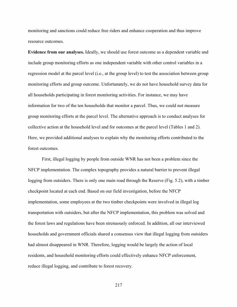
217
monitoring and sanctions could reduce free riders and enhance cooperation and thus improve
resource outcomes.
Evidence from our analyses. Ideally, we should use forest outcome as a dependent variable and
include group monitoring efforts as one independent variable with other control variables in a
regression model at the parcel level (i.e., at the group level) to test the association between group
monitoring efforts and group outcome. Unfortunately, we do not have household survey data for
all households participating in forest monitoring activities. For instance, we may have
information for two of the ten households that monitor a parcel. Thus, we could not measure
group monitoring efforts at the parcel level. The alternative approach is to conduct analyses for
collective action at the household level and for outcomes at the parcel level (Tables 1 and 2).
Here, we provided additional analyses to explain why the monitoring efforts contributed to the
forest outcomes.
First, illegal logging by people from outside WNR has not been a problem since the
NFCP implementation. The complex topography provides a natural barrier to prevent illegal
logging from outsiders. There is only one main road through the Reserve (Fig. 5.2), with a timber
checkpoint located at each end. Based on our field investigation, before the NFCP
implementation, some employees at the two timber checkpoints were involved in illegal log
transportation with outsiders, but after the NFCP implementation, this problem was solved and
the forest laws and regulations have been strenuously enforced. In addition, all our interviewed
households and government officials shared a consensus view that illegal logging from outsiders
had almost disappeared in WNR. Therefore, logging would be largely the action of local
residents, and household monitoring efforts could effectively enhance NFCP enforcement,
reduce illegal logging, and contribute to forest recovery.
218
Second, our results show similar nonlinear effects of group size on both collective action
and resource outcomes (Tables 5.1 and 5.2). This is also indirect evidence to support the
inference that collective action contributed substantially to the outcomes. Since there are no
forest parcels without NFCP monitoring in our study area and surrounding regions, we could not
compare the outcomes between parcels with and without monitoring. However, our study
(Tuanmu, 2012) compared panda habitat recovery rates between household-monitored parcels
and government-monitored parcels. We found that panda habitat recovered faster in household-
monitored parcels than in government-monitored parcels. Because forest is the essential part of
panda habitat, the results supported that household monitoring directly improved forest and
panda habitat recovery. Meanwhile, all our evidence indirectly indicates that, along with
intangible social norms and networks, household monitoring prevents illegal logging and
contributes to forest recovery. In the following sections, we further elucidate how tangible
actions and intangible social norms and networks affected collective action and resource
outcomes.
2.4.2. How do social ties to local leaders affect collective action?
Evidence from literature. Social learning theories suggest that individuals do not imitate
behaviors from others randomly, but rather that leaders will be disproportionally imitated, and
thus have more influence on others’ behaviors (Henrich and Gil-White, 2001; Milinski et al.,
2002; Rustagi et al., 2010). Compared to others, leaders often are elders and/or wealthier, more
educated, prestigious, reputable, powerful (Henrich and Gil-White, 2001; Rustagi et al., 2010).
Therefore, behaviors of leaders would more likely influence other members and thus affect
collective action.

219
Although the detailed mechanisms of how social capital, including social norms, ties, and
networks, affect collective action have not yet been theorized, it is widely recognized that social
capital plays an important role in affecting collective action and resource outcomes (Anthony
and Campbell, 2011; Dietz and Henry, 2008). On one hand, social capital may encourage trust
and communication, ensure rule compliance, reduce monitoring and transaction costs, and thus
enhance collective action (Pretty, 2003). On the other hand, social capital may encourage
political coercion and act as an obstacle to shape inappropriate social arrangements (Adhikari
and Goldey, 2010; Portes and Landolt, 1996).
Evidence from our analyses. To understand why and how social ties to local leaders affect
household monitoring efforts in our case, we first examined what characteristics determine
whether a household has strong or weak social ties to local leaders. Our results suggest that
households with strong social ties to local leaders tend to have a higher average age and
education level of adults (Tables S5.6 and S5.7). Because our measurement of social ties
occurred during the NFCP implementation period, and the birth years and education levels of
adult household members were determined far before the establishment of their social ties to
local leaders, the causal inference can only be that higher average age and education of adult
members help a household to accumulate strong social ties to local leaders rather than vice versa.
Our results (Table 5.1) also suggest that households with strong social ties to local
leaders tended to spend less on monitoring efforts. The reasons are implied by the words of some
household interviewees, for example,
“Almost every household has been assigned to a forest parcel. If you go to cut trees in
others’ parcels and happen to be known by them, it will harm social relationships with
them. … For households with strong social ties to local leaders, we dare not and do not

220
want to offend them because they know more than us, have more social relationships and
power, and we often need to turn to them for help.”
The staff members in the Wolong Administrative Bureau who are in charge of
combatting illegal logging activities are hired from outside WNR (usually college graduates) and
are not related to local residents. In addition, anyone can report illegal logging and receive a cash
reward from the Bureau. We are also not aware of a single case in which staff members have
turned a “blind eye” to illegal logging so households with strong ties to them could avoid
monitoring or sanctions. Thus, these reasons cannot explain why households with strong social
ties to local leaders have less need to monitor. Rather, combining interviewees’ statements and
the analyses above, the reasonable explanation is that households with strong social ties to local
leaders often have more social relationships, power, knowledge, and experience than households
with weak social ties to local leaders, and such social ties provide social capital and repuation
that prevent others from illegal activities in their monitoring parcels. Thus, these households
have less need to monitor.
2.4.3. Is the nonlinear effect on collective action really caused by group size?
To answer this question, we used two approaches to support our argument that the
nonlinear effect is indeed caused by group size and that instrumental variables affect collective
action through group size. Since only the distance from each household to its monitored parcel
and the NFCP payment were linearly associated with group size as criteria in group formation
(Section 1.2, Table S5.2), we used them as hypothesized instrumental variables.
For the first approach, we examined the association type between each hypothesized
instrumental variable and collective action. Our results (Table S5.8) suggest that either the

221
distance from each household to its monitored parcel or the NFCP payment is linearly associated
with collective action. Since all the additional controls are the same as the ones used in the model
of nonlinear group-size effect on collective action (Table 5.1 or Table S5.9), these results suggest
that the two hypothesized instrumental variables cannot explain the nonlinear effect of group size
on collective action. Rather they affect collective action through group size. These results also
support that the group-size distribution in our dataset, although not completely random, is still
suitable to analyze the group-size effects.
For the second approach, we used a two-step Tobit model with endogenous variables.
Using either the instrument of distance from each household to its monitored parcel or the NFCP
payment, our results (Table S5.10) suggest that our instruments are powerful (F-statistic > 47, p
< 0.001) and exogenous (Wald test of exogeneity of p > 0.1). The second-stage regression (Table
S5.11) also suggests that group size has a nonlinear effect on household monitoring efforts,
regardless of using any of the two hypothesized instruments. These results also suggest that the
distance from each household to its monitored parcel and the NFCP payment affect collective
action through group size. Again, this supports that the group formation in our study, which may
not be completely random, does not constitute an impediment to examine group-size effects.
2.4.4. How does group size cause nonlinear effects on collective action and resource
outcomes?
Based on the results of path analysis (Fig. 5.1, Table S5.5), we explained the mechanisms
of how group size affects collective action and resource outcomes through two opposing forces
in the main text. Here we provided additional qualitative evidence from our interviews to support
this conclusion.

222
The causal inference of the mechanisms of nonlinear group-size effects were also
confirmed by our interviewees. One of our household interviewees provided us a vivid example,
expressing a point also made by many other interviewees, of how the cost of social relationship
deterioration for free riders would increase with group size:
“If I do not go to monitor the parcel assigned to our group, only one group member
would complain to me if the parcel is co-monitored by the two of us, but nine other
households may do so if I am in a group of 10 households.”
2.5. Supporting regression models
In this section, we present a more detailed set of the control variables for the results
shown in Tables 1 and 2 in the main text. We also present regression diagnostics and results of
other supporting regression models to support our results that the nonlinear group-size effects are
robust even when we (i) used different combinations of control variables, (ii) did not consider
spatial autocorrelation, and (iii) discarded some edge points (i.e., observations with group sizes
of 1, 15, or 16) from the total set of observations.
To display the distribution of group size and how collective action or resource outcomes
change with group size, we also visualized the nonlinear relationship between group size and
collective action or forest outcomes (Fig. 5.3). However, given the nature of data and methods
we used (i.e., Tobit model for censored data and spatial autoregressive model for data with
spatial autocorrelation), our models are not simple, classic regression models (e.g., OLS
regression). Visually, the actual observations do not fit the predicted lines in the same way as
those in OLS regressions (Daniel et al., 1999).
223
2.5.1. Supporting results and regression diagnostics of Tobit models
For supporting results and diagnostics of all combinations of Tobit models, please see
Tables S5.9, S5.12, and S5.13.
2.5.2. Supporting results and regression diagnostics of spatial autoregressive models
For the construction of the spatial autoregressive model, we compared spatial mixed,
spatial lag, and spatial error models. The coefficient of the spatially lagged dependent variable
(i.e., ρ) was not significant (z-value: – 0.504, p > 0.1) in the mixed model. The coefficient of the
spatial error correlation (i.e., λ) was significant (p < 0.001) in both the mixed model (z-value:
5.691, p < 0.001) and the error model (z-value: 8.553, p < 0.001). Meanwhile, the error model
had the minimum Akaike Information Criteria (AIC) value. The AIC values for the mixed, lag,
error, and OLS models were – 312.89, – 298.14, – 314.56, and – 279.89, respectively. These
results suggest that the error model was most appropriate.
We examined both the linear and nonlinear relationships between group size and the
percent of forest-cover change from 2001 to 2007. The coefficient of group size in the linear
model was nonsignificant (p > 0.1, Table S5.14), which is not surprising given the presence of an
optimum point within the range of the data. Whether we included spatial autocorrelation or not,
the coefficients of both the quadratic and linear terms of group size were significant (Tables
S5.15 and S5.16). But Moran’s I test suggests that spatial autocorrelation should be included
(Table S5.15). Thus we report the results from the spatial autoregressive model in the main text.
We added the cubic term of group size into the model in Table 5.1 (or Table S5.16). It was
nonsignificant (z-value: 0.221, p > 0.1).

224
As mentioned in Section 1.1.1, even excluding parcels with a group size of one, the
quadratic term of group size was still significant (z-value = – 2.460, p < 0.05). Given there was
only one parcel with group size of 15 and one of 16 in our dataset, we also tested the group-size
effects by excluding these two parcels. The nonlinear group-size effect is still significantly
present among the remaining 149 parcels (z-value = – 2.552, p < 0.05 and z-value = – 2.872, p <
0.01 for the quadratic and linear terms of group size, respectively.)

225
Table S5.1. Descriptive statistics of variables for 156 randomly sampled monitoring households. Variable Mean (S.D.)
Total labor input for monitoring (dependent variable, laborer day) 5.23 (6.15)
Group size (number of households) 3.95 (4.15)
Social ties to local leaders (binary: 0 for weak social ties; 1 for strong social ties)
0.15 (0.36)
Distance between each household and its monitored parcel (km) 4.40 (4.82)
Distance between each household and the main road (km) 0.40 (0.60)
Number of household laborers (individual) 1.98 (1.05)
Household size (number of individuals) 3.48 (1.33)
Education of adults (year) 4.80 (2.60)
NFCP payment (yuan) 862.60 (87.27)
Household income (yuan) 27,965.42 (28,637.83)
Percentage of agricultural income 41.69% (28.86%) Table S5.2. Correlation between group size and other biophysical, demographic, and socioeconomic variables. Group size Spearman’s ρ
Distance between each household and its monitored parcel (km) 0.214**
NFCP payment (yuan) 0.522***
Distance between each household and the main road (km) – 0.142
Social ties to local leaders (binary: 0 for weak social ties; 1 for strong social ties) 0.051
Household size (number of individuals) – 0.117
Average age of adults (year) – 0.061
Education of adults (year) 0.114
Number of household laborers (individual) 0.008
Household income (yuan) – 0.021
Per capita household income (yuan) 0.050
Agricultural income (yuan) – 0.162
Percentage of agricultural income – 0.161
Area of cropland (mu, 1 ha = 15 mu) – 0.061
Notes: Tested with 156 randomly sampled households. **p < 0.01;
***p < 0.001.

226
Table S5.3. Descriptive statistics of variables for 151 household-monitored parcels.
Variable Mean (S.D.)
Percent of forest-cover change from 2001 to 2007 (dependent variable) 13.66% (12.50%)
Group size (number of households) 5.32 (3.45)
Parcel size (100 ha) 1.59 (1.37)
Parcel size per household (100 ha per household) 0.33 (0.27)
Elevation (1,000 m, above sea level) 2.42 (0.37)
Slope (radian) 0.53 (0.07)
Wetness (unitless) 10.89 (0.52)
Distance between each parcel and the nearest household (km) 3.79 (4.64)
Distance between each parcel and the main road (km) 2.60 (3.39)
Initial forest cover in 2001 64.21% (31.75%) Table S5.4. Descriptive statistics of characteristics of 113 randomly sampled monitoring households and their assigned groups. Variable Mean (S.D.)
Group characteristics
Within-group enforcement (binary: 0: weak enforcement; 1: strong enforcement) 0.38 (0.49)
Group size (number of households) 7.04 (3.31)
Within-group division (binary: 0: no within-group division; 1: has within-group division) 0.45 (0.50)
Household characteristics
Free rider (binary: 0 for a household that does not free ride; 1 for a household that free rides) 0.24 (0.43)
Social ties to local leaders (binary: 0 for weak social ties; 1 for strong social ties) 0.27 (0.45)
Distance to the main road (km) 0.37 (0.62)
Number of household laborers (number of individuals)
2.53 (1.23)
Household size (number of individuals) 3.68 (1.57)
Education of adults (year) 5.51 (2.76)
Household income (yuan) 34,257.02 (36,296.61)
Percentage of agricultural income 13.74% (21.88%) Notes: Because collective action within each group requires a group having at least two members, here only those groups with at least two members were included for analysis.
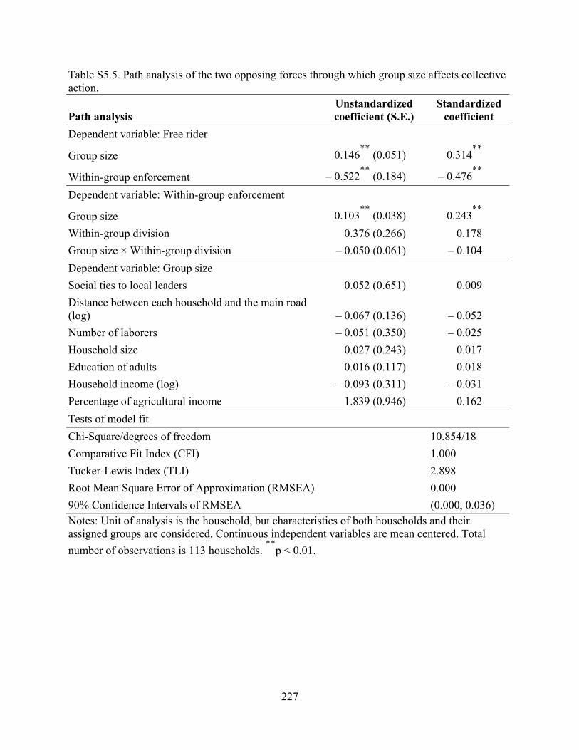
227
Table S5.5. Path analysis of the two opposing forces through which group size affects collective action.
Path analysis Unstandardized coefficient (S.E.)
Standardized coefficient
Dependent variable: Free rider
Group size 0.146**
(0.051) 0.314**
Within-group enforcement – 0.522**
(0.184) – 0.476**
Dependent variable: Within-group enforcement
Group size 0.103**
(0.038) 0.243**
Within-group division 0.376 (0.266) 0.178
Group size × Within-group division – 0.050 (0.061) – 0.104
Dependent variable: Group size
Social ties to local leaders 0.052 (0.651) 0.009
Distance between each household and the main road (log) – 0.067 (0.136) – 0.052
Number of laborers – 0.051 (0.350) – 0.025
Household size 0.027 (0.243) 0.017
Education of adults 0.016 (0.117) 0.018
Household income (log) – 0.093 (0.311) – 0.031
Percentage of agricultural income 1.839 (0.946) 0.162
Tests of model fit
Chi-Square/degrees of freedom 10.854/18
Comparative Fit Index (CFI) 1.000
Tucker-Lewis Index (TLI) 2.898
Root Mean Square Error of Approximation (RMSEA) 0.000
90% Confidence Intervals of RMSEA (0.000, 0.036) Notes: Unit of analysis is the household, but characteristics of both households and their assigned groups are considered. Continuous independent variables are mean centered. Total
number of observations is 113 households. **
p < 0.01.

228
Table S5.6. Characteristics of households with strong and weak social ties to local leaders.
Variable Households with weak social ties
Households with strong social ties
Test statistic (t
value)
Distance between each household and the main road (km) 390.39 (51.89) 424.40 (134.00) – 0.237
Household size (number of individuals) 3.53 (0.12) 3.33 (0.29) 0.638
Percentage of females in adults 0.48 (0.02) 0.47 (0.03) – 0.292
Education of adults (year) 4.55 (0.22) 6.21 (0.58) – 2.904**
Average age of adults (year) 46.31 (0.92) 46.90 (2.07) – 0.263
Household income (yuan) 27,132.16 (2471.90) 32,209.08 (6182.76) – 0.763
Per capita household income (yuan) 8,309.03 (963.20) 10,858.72 (2188.14) – 1.067
Agricultural income (yuan) 11,337.70 (1,455.17)13,173.63 (3,113.16) – 0.534
Percentage of agricultural income 0.42 (0.02) 0.44 (0.07) – 0.209
Area of cropland (Mu, 1 Mu = 1/15 ha) 4.03 (0.21) 4.02 (0.44) – 0.030 Notes: Numbers within parentheses are standard error of mean. The test used was unequal
variance t-test. **
p < 0.01

229
Table S5.7. Logit estimation of factors associated with social ties to local leaders.
Variable Coefficients (Robust S.E.)
Marginal effects
Intercept – 8.711* (3.842) –
Township (dummy) 0.071 (0.488) 0.008
Distance between each household and the main road 0.435(0.503) 0.052
Household size – 0.073 (0.215) – 0.009
Percentage of females in adults – 0.690 (1.219) – 0.082
Education of adults 0.321**
(0.109) 0.038
Average age of adults 0.048* (0.024) 0.006
Household income (log) 0.352 (0.354) 0.042
Percentage of agricultural income 0.255 (0.981) 0.030
Area of cropland – 0.053 (0.121) – 0.006 Notes: Dependent variable is the social ties to local leaders (binary: 0 for weak social ties; 1 for strong social ties). Total number of observations is 156. Log pseudolikelihood is – 60.337.
Pseudo R-squared is 0.099. Variance Inflation Factors were tested to be < 5. *p < 0.05;
**p <
0.01.

230
Table S5.8. Tobit models for hypothesized instrumental variables. Variable Model (1) Model (2) Model (3) Model (4)
Intercept 3.533* (1.568) 2.783 (1.621) 3.328
* (1.388) 3.341
* (1.379)
Distance between each household and its monitored parcel 0.351
* (0.160) 0.130 (0.293) – –
Quadratic term of distance to monitoring parcel – 0.020 (0.021) – –
NFCP payment – – 0.019* (0.008) 0.019
* (0.008)
Quadratic term of NFCP payments – – –
– 8.250 E-06 (1.330 E-05)
Social ties to local leaders (binary)
– 4.365*
(1.857)– 4.206
*
(1.890)– 4.898
*
(1.875) – 4.936
**
(1.875)
Distance between each household and the main road 4.143
** (1.439) 4.089
** (1.430) 3.300
* (1.350) 3.292
* (1.347)
Number of laborers 0.602 (0.830) 0.557 (0.814) 0.386 (0.794) 0.370 (0.797)
Household size – 1.003 (0.678) – 1.034 (0.689) – 0.999 (0.682) – 0.992 (0.681)
Education of adults 0.313 (0.388) 0.273 (0.388) 0.253 (0.398) 0.249 (0.398)
Household income (log) – 0.064 (1.101) – 0.210 (1.111) – 0.022 (1.060) – 0.059 (1.062)
Percentage of agricultural income – 4.398 (3.031) – 4.768 (3.031) – 4.904 (3.045) – 4.875 (3.034)
Sampling weight 0.638 (1.113) 0.823 (1.067) 0.851 (0.914) 0.896 (0.933)
Log pseudolikelihood – 395.934 – 395.530 – 395.465 – 395.381
Pseudo R-Squared 0.023 0.024 0.024 0.024Notes: Unit of analysis is the household. Dependent variable is total labor input for monitoring. Total number of observations is 156. The numbers of left-censored and right-censored observations are 47 and 14, respectively. Independent variables were mean centered. Numbers within parentheses are robust standard errors. For clusters of households from the same monitoring groups, the sampling weight matrix is applied and standard errors are adjusted.
Variance Inflation Factors were tested to be < 5. *p < 0.05;
**p < 0.01;
***p < 0.001.
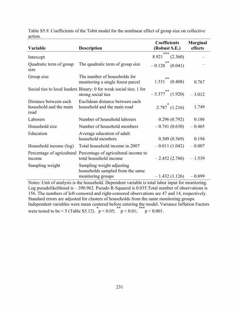
231
Table S5.9. Coefficients of the Tobit model for the nonlinear effect of group size on collective action.
Variable Description Coefficients
(Robust S.E.) Marginal
effects
Intercept 8.921***
(2.360) –
Quadratic term of group size
The quadratic term of group size – 0.128**
(0.041) –
Group size The number of households for monitoring a single forest parcel 1.331
** (0.408) 0.767
Social ties to local leaders Binary: 0 for weak social ties; 1 for strong social ties – 5.377
** (1.920) – 3.012
Distance between each household and the main road
Euclidean distance between each household and the main road 2.787
* (1.216) 1.749
Laborers Number of household laborers 0.296 (0.792) 0.186
Household size Number of household members – 0.741 (0.630) – 0.465
Education Average education of adult household members 0.309 (0.369) 0.194
Household income (log) Total household income in 2007 – 0.011 (1.042) – 0.007
Percentage of agricultural income
Percentage of agricultural income to total household income – 2.452 (2.760) – 1.539
Sampling weight Sampling weight adjusting households sampled from the same monitoring groups – 1.432 (1.126) – 0.899
Notes: Unit of analysis is the household. Dependent variable is total labor input for monitoring. Log pseudolikelihood is – 390.962. Pseudo R-Squared is 0.035.Total number of observations is 156. The numbers of left-censored and right-censored observations are 47 and 14, respectively. Standard errors are adjusted for clusters of households from the same monitoring groups. Independent variables were mean centered before entering the model. Variance Inflation Factors
were tested to be < 5 (Table S5.12). *p < 0.05;
**p < 0.01;
***p < 0.001.

232
Table S5.10. First-stage regression results of the two-step Tobit model. Dependent variable: Group size Model (1) Model (2)
Intercept – 4.178
***
(0.329) – 4.213
***
(0.329)
Distance between each household and its monitored parcel 0.104
** (0.037) –
NFCP payment – 0.007**
(0.002)
Quadratic term of group size 0.098***
(0.008) 0.929***
(0.008)
Social ties to local leaders (binary) 0.755 (0.479) 0.578 (0.465)
Distance between each household and the main road 0.672 (0.319) 0.444 (0.299)
Number of laborers 0.200 (0.213) 0.116 (0.206)
Household size – 0.161*
(0.164) – 0.169*
(0.159)
Education of adults – 0.012 (0.071) 0.035 (0.069)
Household income (log) – 0.027 (0.248) – 0.027 (0.241)
Percentage of agricultural income – 1.285 (0.651) – 1.585† (0.640)
Sampling weight 1.691***
(0.228) 1.800***
(0.220)
F-statistic 47.69***
51.34***
Wald test of exogeneity χ2(1) 1.94 1.74
R-squared 0.767 0.780
Adj. R-Squared 0.751 0.765 Notes: Unit of analysis is the household. Dependent variable is group size. Log pseudolikelihood is – 399.544. Total number of observations is 156. The numbers of left-censored and right-censored observations are 46 and 14, respectively. Independent variables were mean centered before entering the model. Numbers in parentheses are standard errors. For clusters of households from the same monitoring groups, the sampling weight matrix is
applied and standard errors are adjusted. Variance Inflation Factors were tested to be < 5. †p
< 0.1; *p < 0.05;
**p < 0.01;
***p < 0.001.

233
Table S5.11. Second-stage regression results of the two-step Tobit model. Dependent variable: Monitoring efforts Model (1) Model (2)
Intercept 17.267* (7.075) 14.650
** (5.061)
Quadratic term of group size – 0.324† (0.166) – 0.263
* (0.119)
Group size 3.265* (1.602) 2.667
* (1.132)
Social ties to local leaders (binary) – 6.648**
(2.491) – 6.235**
(2.263)
Distance between each household and the main road 1.958 (1.570) 2.195 (1.431)
Number of laborers 0.003 (1.008) 0.108 (1.052)
Household size – 0.484 (0.783) – 0.556 (0.732)
Education of adults 0.367 (0.336) 0.355 (0.319)
Household income (log) – 0.027 (1.141) – 0.010 (1.082)
Percentage of agricultural income – 9.372 (3.461) – 1.001 (3.107)
Sampling weight – 4.850 (3.017) – 3.779† (2.221)
Notes: Models (1) and (2) used distance to monitored parcel and NFCP payment as an instrument, respectively. Unit of analysis is the household. Dependent variable is total labor input for monitoring. Total number of observations is 156. The numbers of left-censored and right-censored observations are 46 and 14, respectively. Independent variables were mean centered before entering the model. Numbers within parentheses are standard errors. For clusters of households from the same monitoring groups, the sampling weight matrix is applied and
standard errors are adjusted. Variance Inflation Factors were tested to be < 5. †p < 0.1;
*p < 0.05;
**p < 0.01;
***p < 0.001.
Table S5.12. Variance inflation factors for variables used in the Tobit model examining the nonlinear group-size effect (Table 5.1 or Table S5.9). Variable Variance Inflation Factor
Group size 2.86
Quadratic term of group size 2.90
Social ties to local leaders 1.07
Distance between each household and the main road 1.24
Laborers 1.98
Household size 1.70
Education 1.21
Household income (log) 1.39
Percentage of agricultural income 1.25 Notes: VIFs should be < 5. Independent variables were mean centered before entering the model.

234
Table S5.13. Different combinations of Tobit models for the nonlinear effect of group size on collective action. Variable Model (1) Model (2) Model (3)
Intercept 8.452***
(2.318) 8.918***
(2.361) 9.074***
(2.353)
Quadratic term of group size – 0.122**
(0.041) – 0.128**
(0.041) – 0.128
**
(0.042)
Group size 1.283**
(0.401) 1.332**
(0.408) 1.369**
(0.414)
Social ties to local leaders (binary) – 5.349**
(1.864) – 5.372**
(1.925) – 5.450
**
(1.907)
Distance between each household and the main road 2.986
* (1.208) 2.785
* (1.218) 2.311
* (1.145)
Laborers 0.227 (0.804) 0.304 (0.792) 0.282 (0.795)
Household size – 0.729 (0.637) – 0.744 (0.652) – 0.706 (0.643)
Education 0.293 (0.358) 0.310 (0.368) 0.326 (0.366)
Percentage of agricultural income – 4.660 (3.993) – 2.449 (2.759) –
Agricultural income (log) –0.283 (0.403) – – 0.006 (0.278)
Income per capita (log) – – 0.015 (1.041) – 0.051 (1.067)
Sampling weight – – 1.429 (1.123) – 1.542 (1.064)
Log pseudolikelihood – 390.62 – 390.962 – 391.364
Pseudo R-squared 0.036 0.035 0.034Notes: Unit of analysis is the household. Dependent variable is total labor input for monitoring. Total number of observations is 156. The numbers of left-censored and right-censored observations are 47 and 14, respectively. For clusters of households from the same monitoring groups, the sampling weight matrix is applied and standard errors are adjusted. Independent variables were mean centered before entering the model. Numbers in parentheses are robust
standard errors. Variance Inflation Factors were tested to be < 5. *p < 0.05;
**p < 0.01;
***p <
0.001.

235
Table S5.14. Coefficients of the spatial autoregressive error model for the linear effect of group size. Variable Coefficients (S.E.)
Intercept 0.132***
(0.014)
Group size 0.002 (0.003)
Parcel size – 0.010 (0.009)
Parcel size per household – 0.001 (0.038)
Elevation 0.050 (0.037)
Slope 0.340**
(0.123)
Wetness 0.0491***
(0.012)
Distance between each parcel and the nearest household 2.828E-04 (0.004)
Distance between each parcel and the main road – 0.002 (0.005)
Initial forest cover in 2001 – 0.263***
(0.030)
Moran’s I 0.023 Notes: Unit of analysis is the parcel. Dependent variable is the percent of forest-cover change from 2001 to 2007. Total number of observations is 151. Log likelihood is 167.942. Variance
Inflation Factors were tested to be < 5. *p < 0.05;
**p < 0.01;
***p < 0.001.

236
Table S5.15. Coefficients of the multiple linear regression for the nonlinear effect of group size. Variable Coefficients (Robust S.E.)
Intercept 0.161**
(0.011)
Group size 0.010* (0.005)
Quadratic term of group size – 0.002**
(0.001)
Parcel size – 0.014 (0.010)
Parcel size per household 0.038 (0.042)
Elevation 0.023 (0.040)
Slope 0.185 (0.110)
Wetness 0.035* (0.021)
Distance between each parcel and the nearest household 0.002 (0.002)
Distance between each parcel and the main road – 0.009* (0.004)
Initial forest cover in 2001 – 0.226**
(0.032)
Moran’s I 0.355**
Notes: Unit of analysis is the parcel. Dependent variable is the percent of forest-cover change from 2001 to 2007. Total number of observations is 151. R-squared is 0.496. Adjusted R-squared is 0.460. Numbers in parentheses are robust standard errors. Variance Inflation Factors were tested to be < 5. The Moran’s I for residuals is significant, indicating the multiple linear
regression is inappropriate and the spatial autocorrelation should be considered. *p < 0.05;
**p <
0.001.

237
Table S5.16. Coefficients of the spatial autoregressive error model for the nonlinear effect of group size on resource outcomes. Variable Description Coefficients (S.E.)
Intercept 0.146***
(0.015)
Quadratic term of group size The quadratic term of group size (household squared) –1.056E-03
* (4.800E-04)
Group size The number of households for monitoring a single forest parcel (household) 7.205E-03
* (3.643E-03)
Parcel size Area of each parcel (100 ha) – 0.013 (0.009)
Parcel size per household Ratio of parcel size to group size (100 ha per household) 0.026 (0.040)
Elevation Average elevation of each parcel (1,000 m, above sea level) 0.034 (0.037)
Slope Average slope of each parcel (radian) 0.339**
(0.121)
Wetness Compound Topographic Index as a measurement of wetness of each parcel (unitless; (Gessler et al., 1995)) 0.048
*** (0.012)
Distance between each parcel and the nearest household
Euclidean distance from each parcel to the nearest household location (km) 4.402E-04 (0.003)
Distance between each parcel and the main road
Euclidean distance from each parcel to the main road (km) – 0.004 (0.005)
Initial forest cover in 2001 Average forest cover of each parcel in 2001 – 0.269
*** (0.030)
λ Spatial error correlation coefficient 0.561***
Moran’s I Moran’s I test of spatial autocorrelation for model residuals 0.021
Notes: Unit of analysis is the parcel. Dependent variable is the percent of forest-cover change from 2001 to 2007. Log likelihood is 170.281. Total number of observations is 151. Independent variables were mean centered before entering the model. Variance Inflation Factors were tested
to be < 5 (Table S5.17). *p < 0.05;
**p < 0.01;
***p < 0.001.

238
Table S5.17. Variance inflation factors (VIFs) for variables used in the spatial simultaneous autoregressive error model (Table 5.1 or Table S5.16). Variable Variance Inflation Factor
Group size 4.01
Quadratic term of group size 1.89
Parcel size 4.07
Parcel size per household 3.09
Elevation 3.54
Slope 1.44
Wetness 1.18
Distance between each parcel and the nearest household 2.09
Distance between each parcel and the main road 3.51
Initial forest cover in 2001 1.42 Notes: VIFs were tested to be < 5. Independent variables were mean centered before entering the model.

239
APPENDIX E
SUPPORTING INFORMATION FOR CHAPTER 6
Centered polynomial regression is a common technique to reduce the collinearity
between components and the product terms that represent interaction or nonlinear effects (Aiken
and West, 1991; Dalal and Zickar, 2012). Often mean-centering is used, it does not change the fit
of regression models, does not affect the power to detect interaction or nonlinear effects, does
not alter the reliability of product terms, and does not change the highest order coefficients. But
it does change the coefficients of lower order terms (and thus the best-fit values at peaks and
valleys of the curve), standard errors, and confidence intervals, as well as improve the
interpretation. Here we provided a brief proof to clarify the changes of coefficients and
improvements in interpretation. For a detailed discussion, please see cited references (Aiken and
West, 1991; Dalal and Zickar, 2012).
The general form of uncentered polynomial regression with first order terms and
multiplicative interaction term is given as (Aiken and West, 1991; Dalal and Zickar, 2012):
Y = b0 + b1X1 + b2X2 + b3X1X2 + ξ (6.2.1)
where Y is the dependent variable; X1 and X2 are independent variables; X1X2 is the
multiplicative interaction term; b0 is the intercept; b1 and b2 are coefficients to be estimated; ξ is
the error term that has a normal distribution with mean of zero. When X1 = X2, the multiplicative
interaction term becomes the quadratic term.

240
After mean-centering X1 and X2 in Equation 6.2.1, the equation of centered polynomial
regression is given as:
221132221110 XXXXbXXbXXbbY (6.2.2)
where 1X and 2X are the means of X1 and X2, respectively; 2211 XXXX is the
multiplicative interaction term of X1 and X2 after mean-centering.
Equation 6.2.2 can be rearranged and factored into Equation 6.2.3:
2132132123121322110 XXbXXbbXXbbXXbXbXbbY (6.2.3)
Comparing Equation 6.2.1 and 6.2.3, it is easy to see that the coefficient of the interaction
term (X1X2) does not change; however, the intercept and coefficients for first order terms (X1
and X2) do alter in a predictable way. From Equation 6.2.2, it is also easy to see that the
interpretation of marginal effects [also called conditional or simple effects for polynomial
regressions(Dalal and Zickar, 2012)] become easy since b1 and b2 are actually the marginal
effects of X1 and X2 at the mean values of X2 and X1, respectively.

241
Table S6.1. Descriptive statistics of variables used in modeling the effects of conservation and development policies on changes in total household income and income structure. Variables Description
Mean (S.D.)
Dependent variable for the model in Table 6.1
Changes in total household income
The difference of total household income in 2007 subtracting total household income in 1998 ( thousand yuan)
21.988 (27.286)
Dependent variable for the model in Table 6.2
Changes in the percentage of agricultural income
The difference of percentage of agricultural income in 2007 subtracting the percentage of agricultural income in 1998
–0.218 (0.389)
Policy intervention NFCP payment The payment each household received annually from the NFCP ( thousand yuan)
0.948 (0.183)
NFCP payment percentage
NFCP payment divided by total household income in 2007
0.065 (0.060)
GTGB payment
The payment each household received annually from the cropland conversion policies (i.e., GTGP and GTBP) ( thousand yuan)
2.888 (2.320)
GTGB payment percentage
GTGB payment divided by total household income in 2007
0.160 (0.153)
Tourism participation
Household participation in tourism business (1: participated; 0: not participated)
0.274 (0.447)
Electricity subsidy Initial subsidy received for electricity consumption (yuan)
85.982 (104.429)
Electricity subsidy percentage
NFCP payment divided by total household income in 1998 (‰)
0.027 (0.041)

242
Table S6.1 (cont’d) Variables Description
Mean (S.D.)
Financial capital Initial total household income
Total household income in 1998 (thousand yuan)
6.285 (4.932)
Initial percentage of agricultural income
The percentage of agricultural income in 1998
0.630 (0.313)
Changes in total agricultural income
The difference of total agricultural income in 2007 subtracting total agricultural income in 1998 (thousand yuan)
7.817 (15.393)
Human capital Number of laborers The number of laborers in each household
2.820 (1.455)
Changes in number of laborers
The difference of number of laborers in 2007 subtracting the number of laborers in 1998
–0.727 (1.795)
Education Education level of the most educated non-student adult in 2007 (year)
7.120 (3.432)
Natural capital Cropland area The total area of cropland for each household in 2007 (Mu, 1 Mu = 1/15 ha)
10.450 (4.163)
Built-up capital Distance to the main road
The Euclidean distance from each household location to the main road (km)
0.431 (0.629)
Social capital Social ties to local governments
Whether the household has a member of immediate relative working in local governments or government enterprises: 1. Yes; 0: No.
0.120 (0.326)
Notes: All monetary values in 1998 are discounted into present values in 2007. The number of observations is 179.

243
Table S6.2. Complementary results of the effects of conservation and development policies on changes in total household income. Variables
Unstandardized coefficients
Standardized coefficients
Robust S.E.
Policy intervention
NFCP payment –4.816 –0.021 19.066
GTGB payment 1.925**
0.163**
0.694
Initial electricity subsidy 44.577* 0.171
* 22.335
Tourism participation 11.905**
0.195**
3.934
NFCP payment × GTGB payment 3.985 0.035 11.219
NFCP payment × Initial electricity subsidy
–0.050 –0.016 0.144
NFCP payment × Tourism participation –116.000
* –0.134
* 48.657
GTGB payment × Tourism participation
1.505 0.083 2.265
GTGB payment × Initial electricity subsidy
0.005 0.038 0.009
Financial capital
Initial total household income –0.401 –0.072 0.326
Changes in total agricultural income 1.253
*** 0.712
*** 0.241
Human capital
Number of laborers 3.295* 0.177
* 1.513
Changes in number of laborers 2.610* 0.173
* 1.116
Education 0.266 0.033 0.431
Natural capital
Cropland area –0.313 –0.028 0.646
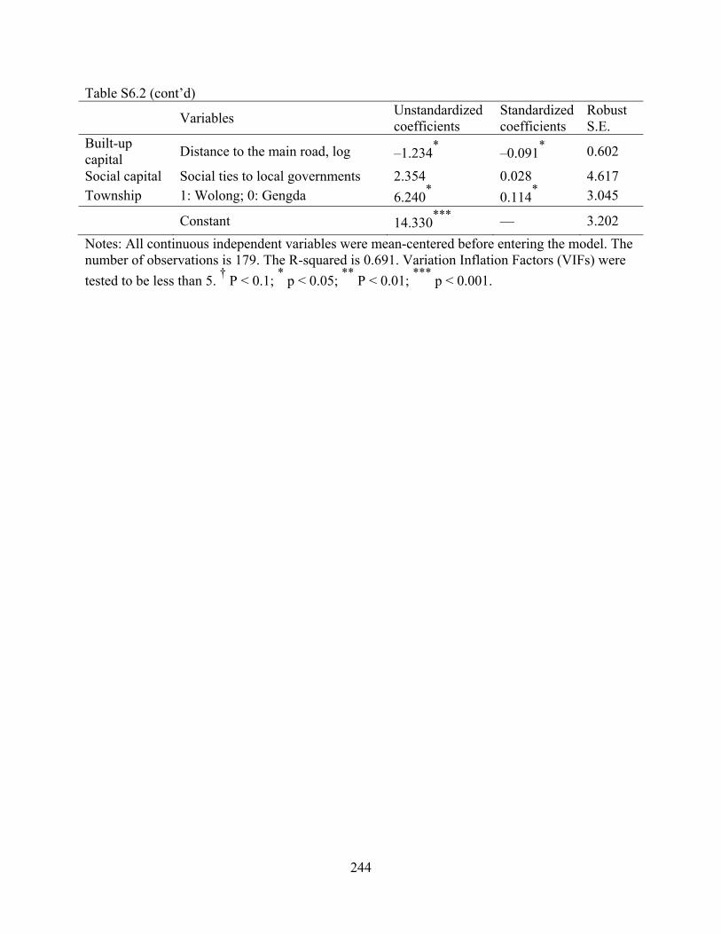
244
Table S6.2 (cont’d) Variables
Unstandardized coefficients
Standardized coefficients
Robust S.E.
Built-up capital
Distance to the main road, log –1.234* –0.091
* 0.602
Social capital Social ties to local governments 2.354 0.028 4.617 Township 1: Wolong; 0: Gengda 6.240
* 0.114
* 3.045
Constant 14.330***
— 3.202
Notes: All continuous independent variables were mean-centered before entering the model. The number of observations is 179. The R-squared is 0.691. Variation Inflation Factors (VIFs) were
tested to be less than 5. † P < 0.1;
* p < 0.05;
** P < 0.01;
*** p < 0.001.

245
Table S6.3. Complementary results of the effects of conservation and development policies on changes in the percentage of agricultural income. Variables
Unstandardized coefficients
Standardized coefficients
Robust S.E.
Policy intervention
NFCP payment –0.068 –0.020 0.196
GTGB payment –0.037***
–0.221***
0.009
NFCP payment × GTGB payment
–0.088 –0.054 0.098
Initial electricity subsidy –3.262e-04* –0.088
*
1.355e-04
Tourism participation –0.096* –0.110
* 0.047
NFCP payment × Initial electricity subsidy
–8.83e-04 –0.020 0.002
NFCP payment × Tourism participation 1.526
* 0.123
* 0.752
GTGB payment × Initial electricity subsidy
6.07e-05 0.032 4.70e-05
GTGB payment × Tourism participation
0.009 0.036 0.014
Financial capital Initial total household income 0.007* 0.088
* 0.004
Initial agricultural income percentage –0.862
*** –0.687
*** 0.057
Changes in total agricultural income 0.007
** 0.277
** 0.002
Human capital Number of laborers 0.026 0.099 0.022 Changes in number of laborers 0.003 0.013 0.015
Education –0.007 –0.060 0.005
Natural capital Cropland area 0.023**
0.147***
0.008
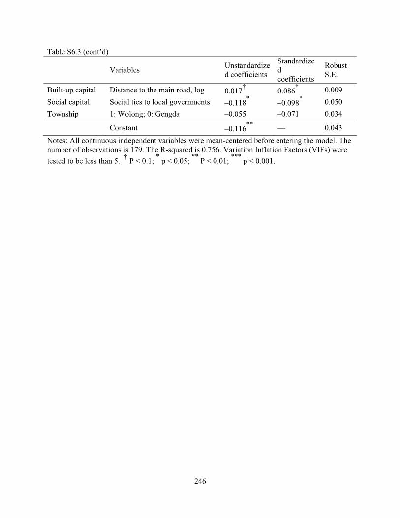
246
Table S6.3 (cont’d)
Variables Unstandardized coefficients
Standardized coefficients
Robust S.E.
Built-up capital Distance to the main road, log 0.017† 0.086
† 0.009
Social capital Social ties to local governments –0.118* –0.098
* 0.050
Township 1: Wolong; 0: Gengda –0.055 –0.071 0.034 Constant –0.116
** — 0.043
Notes: All continuous independent variables were mean-centered before entering the model. The number of observations is 179. The R-squared is 0.756. Variation Inflation Factors (VIFs) were
tested to be less than 5. † P < 0.1;
* p < 0.05;
** P < 0.01;
*** p < 0.001.

247
REFERENCES

248
REFERENCES
Abdallah, S., Thompson, S., Marks, N., 2008. Estimating worldwide life satisfaction. Ecol. Econ. 65, 35-47.
Adams, W.M., Aveling, R., Brockington, D., Dickson, B., Elliott, J., Hutton, J., Roe, D., Vira, B., Wolmer, W., 2004. Biodiversity conservation and the eradication of poverty. Science 306, 1146-1149.
Adhikari, K.P., Goldey, P., 2010. Social Capital and its "Downside": The Impact on Sustainability of Induced Community-Based Organizations in Nepal. World Devel. 38, 184-194.
Agrawal, A., 2000. Small is Beautiful, but is Larger Better? Forest Management Institutions in the Kumaon Himalaya, India, in: Gibson, C., McKean, M.A., Ostrom, E. (Eds.), People and Forests: Communities, Institutions, and Governance. MIT Press, Cambridge, pp. 57-85.
Agrawal, A., Chhatre, A., 2006. Explaining success on the commons: Community forest governance in the Indian Himalaya. World Devel. 34, 149-166.
Agrawal, A., Goyal, S., 2001. Group size and collective action - Third-party monitoring in common-pool resources. Comp Polit Stud 34, 63-93.
Aiken, L.S., West, S.G., 1991. Multiple regression: Testing and interpreting interactions. Sage Publications, Incorporated.
Alix-Garcia, J., De Janvry, A., Sadoulet, E., 2008. The role of deforestation risk and calibrated compensation in designing payments for environmental services. Environ. Devel. Econ. 13, 375-394.
An, L., He, G., Liang, Z., Liu, J., 2006. Impacts of demographic and socioeconomic factors on spatio-temporal dynamics of panda habitat. Biodivers. Conserv. 15, 2343-2363.
An, L., Liu, J., Ouyang, Z., Linderman, M., Zhou, S., Zhang, H., 2001. Simulating demographic and socioeconomic processes on household level and implications for giant panda habitats. Ecol. Model. 140, 31-49.
An, L., Lupi, F., Liu, J., Linderman, M.A., Huang, J., 2002. Modeling the choice to switch from fuelwood to electricity: Implications for giant panda habitat conservation. Ecol. Econ. 42, 445-457.
An, L., Mertig, A.G., Liu, J., 2003. Adolescents leaving parental home: Psychosocial correlates and implications for conservation. Population and Environment 24, 415-444.
Anselin, L., 1988. Spatial Econometrics: Methods and Models. Kluwer Academic Publishers Norwell, MA.

249
Anselin, L., Syabri, I., Kho, Y., 2006. GeoDa: An introduction to spatial data analysis. Geographical Analysis 38, 5-22.
Anthony, D.L., Campbell, J.L., 2011. States, social capital and cooperation: looking back on Governing the Commons. International Journal of the Commons 5, 284-302.
Arriagada, R.A., Sills, E.O., Pattanayak, S.K., Ferraro, P.J., 2009. Combining qualitative and quantitative methods to evaluate participation in Costa Rica's Program of payments for environmental services. Journal of Sustainable Forestry 28, 343-367.
Axinn, W.G., Pearce, L.D., Ghimire, D., 1999. Innovations in life history calendar applications. Soc. Sci. Res. 28, 243-264.
Baland, J.-M., Platteau, J.-P., 1996. Halting degradation of natural resources: is there a role for rural communities? Food and Agriculture Organization of the United Nations, Oxford.
Baland, J.M., Platteau, J.P., 1999. The ambiguous impact of inequality on local resource management. World Devel. 27, 773-788.
Barbier, E.B., 2011. Pricing Nature. Annual Review of Resource Economics 3, 337-353.
Barrett, C.B., Travis, A.J., Dasgupta, P., 2011. On biodiversity conservation and poverty traps. Proc. Natl. Acad. Sci. U. S. A. 108, 13907-13912.
Bateman, I.J., Mace, G.M., Fezzi, C., Atkinson, G., Turner, K., 2011. Economic Analysis for Ecosystem Service Assessments. Environ. Resour. Econ. 48, 177-218.
Bearer, S., Linderman, M., Huang, J.Y., An, L., He, G.M., Liu, J.Q., 2008. Effects of fuelwood collection and timber harvesting on giant panda habitat use. Biol. Conserv. 141, 385-393.
Berke, P.R., Campanella, T.J., 2006. Planning for postdisaster resiliency. Ann. Am. Acad. Pol. Soc. Sci. 604, 192-207.
Berkes, F., 2007. Community-based conservation in a globalized world. Proceedings of the National Academy of Sciences 104, 15188-15193.
Berry, P.A.M., Garlick, J.D., Smith, R.G., 2007. Near-global validation of the SRTM DEM using satellite radar altimetry. Remote Sens. Environ. 106, 17-27.
Birch, J.C., Newton, A.C., Aquino, C.A., Cantarello, E., Echeverria, C., Kitzberger, T., Schiappacasse, I., Garavito, N.T., 2010. Cost-effectiveness of dryland forest restoration evaluated by spatial analysis of ecosystem services. Proc. Natl. Acad. Sci. USA 107, 21925-21930.
Blalock, H.M., 1965. Theory Building and the Statistical Concept of Interaction. Am. Sociol. Rev. 30, 374-380.

250
Boardman, A.E., Greenberg, D.H., Vining, A.R., Weimer, D.L., 2006. Cost-Benefit Analysis: Concepts and Practice, 3rd ed. Prentice Hall, Upper Saddle River, New Jersey.
Bollen, K.A., Noble, M.D., 2011. Structural equation models and the quantification of behavior. Proc. Natl. Acad. Sci. U. S. A. 108, 15639-15646.
Bouma, J., Bulte, E., van Soest, D., 2008. Trust and cooperation: Social capital and community resource management. J. Environ. Econ. Manage. 56, 155-166.
Boyd, J., Banzhaf, S., 2007. What are ecosystem services? The need for standardized environmental accounting units. Ecol. Econ. 63, 616-626.
Boyd, R., Gintis, H., Bowles, S., 2010. Coordinated Punishment of Defectors Sustains Cooperation and Can Proliferate When Rare. Science 328, 617-620.
Brown, T.A., 2006. Confirmatory factor analysis for applied research. The Guilford Press, New York, NY.
Butler, C.D., Oluoch-Kosura, W., 2006. Linking future ecosystem services and future human well-being. Ecol. Soc. 11, 30.
Cai, J., Jiang, Z.G., Zeng, Y., Li, C.W., Bravery, B.D., 2008. Factors affecting crop damage by wild boar and methods of mitigation in a giant panda reserve. Eur J Wildl Res 54, 723-728.
Camfield, L., Skevington, S.M., 2008. On subjective well-being and quality of life. Journal of Health Psychology 13, 764-775.
Campbell, A., 1976. Subjective Measures of Well-Being. Am. Psychol. 31, 117-124.
Carpenter, J.P., 2007. Punishing free-riders: How group size affects mutual monitoring and the provision of public goods. Games Econ. Behav. 60, 31-51.
Carpenter, S.R., DeFries, R., Dietz, T., Mooney, H.A., Polasky, S., Reid, W.V., Scholes, R.J., 2006. Millennium Ecosystem Assessment: Research Needs. Science 314, 257-258.
Carpenter, S.R., Mooney, H.A., Agard, J., Capistrano, D., DeFries, R.S., Diaz, S., Dietz, T., Duraiappah, A.K., Oteng-Yeboah, A., Pereira, H.M., Perrings, C., Reid, W.V., Sarukhan, J., Scholes, R.J., Whyte, A., 2009. Science for managing ecosystem services: Beyond the Millennium Ecosystem Assessment. Proc. Natl. Acad. Sci. U. S. A. 106, 1305-1312.
Chamberlin, J.R., 1974. Provision of Collective Goods as a Function of Group Size. Amer. Polit. Sci. Rev. 68, 707-716.
Chang, J., Wu, X., Liu, A.Q., Wang, Y., Xu, B., Yang, W., Meyerson, L.A., Gu, B.J., Peng, C.H., Ge, Y., 2011. Assessment of net ecosystem services of plastic greenhouse vegetable cultivation in China. Ecol. Econ. 70, 740-748.

251
Chee, Y.E., 2004. An ecological perspective on the valuation of ecosystem services. Biol. Conserv. 120, 549-565.
Chen, X., Frank, K.A., Dietz, T., Liu, J., 2012a. Weak ties, labor Migration, and environmental impacts: Toward a sociology of sustainability. Organ. Environ. 25, 3-24.
Chen, X., Lupi, F., An, L., Sheely, R., Viña, A., Liu, J., 2012b. Agent-based modeling of the effects of social norms on enrollment in payments for ecosystem services. Ecological Modeling 229, 16-24.
Chen, X., Lupi, F., He, G., Liu, J., 2009. Linking social norms to efficient conservation investment in payments for ecosystem services. Proc. Natl. Acad. Sci. USA 106, 11812-11817.
Chen, X., Lupi, F., Vina, A., He, G., Liu, J., 2010. Using Cost-Effective Targeting to Enhance the Efficiency of Conservation Investments in Payments for Ecosystem Services. Conserv. Biol. 24, 1469-1478.
Chhatre, A., Agrawal, A., 2008. Forest commons and local enforcement. Proc. Natl. Acad. Sci. USA 105, 13286-13291.
Colby, M.E., 1991. Environmental management in development: the evolution of paradigms. Ecol. Econ. 3, 193-213.
Collins, S.L., Carpenter, S.R., Swinton, S.M., Orenstein, D.E., Childers, D.L., Gragson, T.L., Grimm, N.B., Grove, M., Harlan, S.L., Kaye, J.P., Knapp, A.K., Kofinas, G.P., Magnuson, J.J., McDowell, W.H., Melack, J.M., Ogden, L.A., Robertson, G.P., Smith, M.D., Whitmer, A.C., 2011. An integrated conceptual framework for long-term social-ecological research. Front. Ecol. Environ. 9, 351-357.
Costanza, R., d'Arge, R., de Groot, R., Farber, S., Grasso, M., Hannon, B., Limburg, K., Naeem, S., O'Neill, R.V., Paruelo, J., Raskin, R.G., Sutton, P., van den Belt, M., 1997. The value of the world's ecosystem services and natural capital. Nature 387, 253-260.
Daily, G.C., 1997. Nature's Services: Societal Dependence on natural Ecosystems. Island Press, Washington, D.C.
Daily, G.C., Matson, P.A., 2008. Ecosystem services: From theory to implementation. Proc. Natl. Acad. Sci. U. S. A. 105, 9455-9456.
Dalal, D.K., Zickar, M.J., 2012. Some Common Myths About Centering Predictor Variables in Moderated Multiple Regression and Polynomial Regression. Organ Res Methods 15, 339-362.
Daniel, C., Wood, F.S., Gorman, J.W., 1999. Fitting Equations to Data: Computer Analysis of Multifactor Data. Wiley.
Daniels, A.E., Bagstad, K., Esposito, V., Moulaert, A., Rodriguez, C.M., 2010. Understanding the impacts of Costa Rica's PES: Are we asking the right questions? Ecol. Econ. 69, 2116-2126.

252
De Rus, G., 2010. Introduction to Cost-benefit Analysis: Looking for Reasonable Shortcuts. Edward Elgar Pub.
Diener, E., 1994. Assessing Subjective Well-Being - Progress and Opportunities. Soc. Indic. Res. 31, 103-157.
Diener, E., 2000. Subjective well-being — The science of happiness and a proposal for a national index. Am. Psychol. 55, 34-43.
Diener, E., 2009. The science of well-being: The collected works of Ed Diener. Springer, The Netherlands.
Diener, E., Ryan, K., 2009. Subjective well-being: a general overview. South African Journal of Psychology 39, 391-406.
Diener, E., Suh, E.M., Lucas, R.E., Smith, H.L., 1999. Subjective well-being: Three decades of progress. Psychol. Bull. 125, 276-302.
Dietz, T., Henry, A.D., 2008. Context and the commons. Proc. Natl. Acad. Sci. USA 105, 13189-13190.
Dietz, T., Rosa, E.A., York, R., 2009. Environmentally Efficient Well-Being: Rethinking Sustainability as the Relationship between Human Well-being and Environmental Impacts. Hum. Ecol. Rev. 16, 114-123.
Dietz, T., Rosa, E.A., York, R., 2012. Environmentally efficient well-being: Is there a Kuznets curve? Appl Geogr 32, 21-28.
Eagly, A.H., Kulesa, P., 1997. Attitudes, attitude structure, and resistance to change: implications for persuasion on environmental issues, in: Bazerman, M.H., Messick, D.M., Tenbrunsel, A.E., Wade-Benzoni, K.A. (Eds.), Environmental ethics and behavior. The New Lexington Press, San Francisco, CA, pp. 122-153.
Ekin, P., 2008. The four-capital method of sustainable development evaluation. European Environment 18, 63-80.
Elliott, J.R., Pais, J., 2006. Race, class, and Hurricane Katrina: Social differences in human responses to disaster. Soc. Sci. Res. 35, 295-321.
Engel, S., Pagiola, S., Wunder, S., 2008. Designing payments for environmental services in theory and practice: An overview of the issues. Ecol. Econ. 65, 663-674.
Escobar, A., 1999. After Nature: Steps to an Antiessentialist Political Ecology. Curr Anthrop 40, 1-30.
Esteban, J., Ray, D., 2001. Collective action and the group size paradox. Amer. Polit. Sci. Rev. 95, 663-672.

253
Evenson, R.E., Mwabu, G., 1996. Household composition and expenditures on human capital formation in Kenya. Res Popul Econ 8, 205-232.
Farber, S.C., Costanza, R., Wilson, M.A., 2002. Economic and ecological concepts for valuing ecosystem services. Ecol. Econ. 41, 375-392.
Fehr, E., Gachter, S., 2002. Altruistic punishment in humans. Nature 415, 137-140.
Fischbacher, U., Gachter, S., Fehr, E., 2001. Are people conditionally cooperative? Evidence from a public goods experiment. Econ. Letters 71, 397-404.
Fisher, B., Turner, R.K., Morling, P., 2009. Defining and classifying ecosystem services for decision making. Ecol. Econ. 68, 643-653.
Foley, J.A., DeFries, R., Asner, G.P., Barford, C., Bonan, G., Carpenter, S.R., Chapin, F.S., Coe, M.T., Daily, G.C., Gibbs, H.K., Helkowski, J.H., Holloway, T., Howard, E.A., Kucharik, C.J., Monfreda, C., Patz, J.A., Prentice, I.C., Ramankutty, N., Snyder, P.K., 2005. Global Consequences of Land Use. Science 309, 570-574.
FONAFIFO, CONAFOR, Ministry of Environment, 2012. Lessons learned for REDD+ from PES and conservation incentive programs. Examples from Costa Rica, Mexico, and Ecuador. Costa Rica, Ecuador, Mexico, World Bank, Forest Trends and PROFOR, p. 164.
Forestry Department of Food and Agriculture Organization of the United Nations, 2010. Global Forest Resources Assessment 2010: Country Report - China. Forestry Department of Food and Agriculture Organization of the United Nations, Rome.
Fox, J., 1997. Applied Regression Analysis, Linear Models and Related Methods. SAGE Publications, Inc., Thousand Oaks.
Freeman, D., Thornton, A., Camburn, D., Alwin, D., Yooung-DeMacro, L., 1988. The life history calendar: A technique for collecting retrospective data, in: Clogg, C. (Ed.), Soc. Method. American Sociological Association, Washington, DC., pp. 37-68.
Friedrich, R.J., 1982. In Defense of Multiplicative Terms in Multiple-Regression Equations. Am. J. Polit. Sci. 26, 797-833.
Gallopin, G.C., 2006. Linkages between vulnerability, resilience, and adaptive capacity. Global Environ Chang 16, 293-303.
Gautam, A.P., 2007. Group size, heterogeneity and collective action outcomes: Evidence from community forestry in Nepal. Int J Sustain Dev World Ecol 14, 574-583.
Gefen, D., Straub, D.W., Boudreau, M.-C., 2000. Structural Equation Modeling and Regression: Guidelines for Research Practice Communications of the Association for Information Systems 4, 1-79.

254
Gessler, P.E., Moore, I.D., McKenzie, N.J., Ryan, P.J., 1995. Soil-landscape modeling and spatial prediction of soil attributes. Int J Geogr Inf Sci 9, 421-432.
Gibson, C.C., Williams, J.T., Ostrom, E., 2005. Local enforcement and better forests. World Devel. 33, 273-284.
Grant, S., Langan-Fox, J., Anglim, J., 2009. The Big Five Traits as Predictors of Subjective and Psychological Well-Being. Psychol. Rep. 105, 205-231.
Grigg, A., 2008. Dependency and impact on ecosystem services – unmanaged risk, unrealised opportunity: A briefing document for the food, beverage and tobacco sectors. Fauna & Flora International.
Gross-Camp, N.D., Martin, A., McGuire, S., Kebede, B., Munyarukaza, J., 2012. Payments for ecosystem services in an African protected area: exploring issues of legitimacy, fairness, equity and effectiveness. Oryx 46, 24-33.
Gunderson, L., 2010. Ecological and Human Community Resilience in Response to Natural Disasters. Ecol. Soc. 15, 18.
Haan, M., Kooreman, P., 2002. Free riding and the provision of candy bars. J. Public Econ. 83, 277-291.
Hanley, N., MacMillan, D., Wright, R.E., Bullock, C., Simpson, I., Parsisson, D., Crabtree, B., 1998. Contingent valuation versus choice experiments: Estimating the benefits of environmentally sensitive areas in Scotland. J. Agr. Econ. 49, 1-15.
Hanley, N., Shogren, J.F., White, B., 2001. Introduction to Environmental Economics. Oxford University Press, New York.
Hardin, G., 1968. The Tragedy of the Commons. Science 162, 1243-1248.
He, G., Chen, X., Bearer, S., Colunga, M., Mertig, A., An, L., Zhou, S., Linderman, M., Ouyang, Z., Gage, S., Li, S., Liu, J., 2009. Spatial and temporal patterns of fuel collection in Wolong Nature Reserve: Implications for panda conservation. Landscape Urban Plann. 92, 1-9.
He, G., Chen, X., Liu, W., Bearer, S., Zhou, S., Cheng, L., Zhang, H., Ouyang, Z., Liu, J., 2008. Distribution of Economic Benefits from Ecotourism: A Case Study of Wolong Nature Reserve for Giant Pandas in China. Environ. Manage. 42, 1017-1025.
Henrich, J., Gil-White, F.J., 2001. The evolution of prestige - Freely conferred deference as a mechanism for enhancing the benefits of cultural transmission. Evol Hum Behav 22, 165-196.
Houck, O.A., 1985. Rising water: the national flood insurance program and Louisiana. Tul. L. Rev. 60, 61-164.

255
Hughes, R., Flintan, F., 2001. Integrating Conservation and Development Experience: A Review and Bibliography of the ICDP Literature. International Institute for Environment and Development, London.
Hull, V., Xu, W.H., Liu, W., Zhou, S.Q., Vina, A., Zhang, J.D., Tuanmu, M.N., Huang, J.Y., Linderman, M., Chen, X.D., Huang, Y., Ouyang, Z.Y., Zhang, H.M., Liu, J.G., 2011. Evaluating the efficacy of zoning designations for protected area management. Biol. Conserv. 144, 3028-3037.
Hwang, S.-H., 2011. Larger groups may alleviate collective action problems [Version: 2011.10.11]. Research Institute for Market Economy, Sogang University, Seoul, Korea.
IPCC, 2012. Managing the risks of extreme events and disasters to advance climate change adaption, in: Field, C.B., V. Barros, T.F. Stocker,, D. Qin, D.J.D., K.L. Ebi, M.D. Mastrandrea, K.J. Mach, G.-K. Plattner, S.K. Allen,, M. Tignor, a.P.M.M. (Eds.), A Special Report of Working Groups I and II of the Intergovernmental Panel on Climate Change. Cambridge University Press, New York, NY, USA.
Isaac, R.M., Walker, J.M., Williams, A.W., 1994. Group Size and the Voluntary Provision of Public Goods: Experimental Evidence Utilizing Large Groups. J. Public Econ. 54, 1-36.
IUCN, 1980. World Conservation Strategy: Living Resource Conservation for Sustainable Development. International Union for Conservation of Nature and Natural Resources, Gland, Switzerland.
IUCN, UNEP-WCMC, 2012. The World Database on Protected Areas (WDPA), Februrary 2012 ed. United Nations Environment Programme (UNEP) - World Conservation Monitoring Centre (WCMC), Cambridge, UK.
Jack, B.K., Kousky, C., Sims, K.R.E., 2008. Designing payments for ecosystem services: Lessons from previous experience with incentive-based mechanisms. Proc. Natl. Acad. Sci. U. S. A. 105, 9465-9470.
Jeanrenaud, S., 2002. People-oriented approaches in global conservation: is the leopard changing its spots? International Institute for Environment and Development, London.
Jensen, J.R., 1996. Introductory digital image processing, a remote sensing perspective, Second ed. Prentice Hall, New Jersey.
Jordan, S.J., Hayes, S.E., Yoskowitz, D., Smith, L.M., Summers, J.K., Russell, M., Benson, W.H., 2010. Accounting for natural resources and environmental sustainability: linking ecosystem services to human well-being. Environ. Sci. Technol. 44, 1530-1536.
Kahneman, D., Krueger, A.B., 2006. Developments in the measurement of subjective well-being. J. Econ. Perspect. 20, 3-24.

256
Kalacska, M., Sanchez-Azofeifa, G.A., Rivard, B., Calvo-Alvarado, J.C., Quesada, M., 2008. Baseline assessment for environmental services payments from satellite imagery: A case study from Costa Rica and Mexico. J. Environ. Manage. 88, 348-359.
Kareiva, P., Tallis, H., Ricketts, T.H., Daily, G.C., Polasky, S., 2011. Natural Capital: Theory and Practice of Mapping Ecosystem Services. Oxford University Press.
Kates, R.W., Travis, W.R., Wilbanks, T.J., 2012. Transformational adaptation when incremental adaptations to climate change are insufficient. Proc. Natl. Acad. Sci. U. S. A. 109, 7156-7161.
Kinzig, A.P., Perrings, C., Chapin, F.S., Polasky, S., Smith, V.K., Tilman, D., Turner, B.L., 2011. Paying for Ecosystem Services-Promise and Peril. Science 334, 603-604.
Kiss, A., 2004. Is community-based ecotourism a good use of biodiversity conservation funds? Trends Ecol. Evol. 19, 232-237.
Klein, C.A., Zellmer, S.B., 2007. Mississippi River stories: lessons from a century of unnatural disasters. Southern Methodist University Law Review 60, 1471-1538.
LeSage, J., Pace, R.K., 2009. Introduction to Spatial Econometrics. CRC Press, Boca Raton.
Li, J., Feldman, M.W., Li, S.Z., Daily, G.C., 2011. Rural household income and inequality under the Sloping Land Conversion Program in western China. Proc. Natl. Acad. Sci. U. S. A. 108, 7721-7726.
Li, W., Zhao, X., 1989. China's Nature Reserves. Foreign Language Press, Beijing.
Li, Y., Viña, A., Yang, W., Chen, X., Zhang, J., Ouyang, Z., Liu, J., 2013. Effects of conservation policies on forest cover change in panda habitat regions, China. Land Use Policy 33, 42-53.
Lichstein, J.W., Simons, T.R., Shriner, S.A., Franzreb, K.E., 2002. Spatial autocorrelation and autoregressive models in ecology. Ecol. Monogr. 72, 445-463.
Lin, N., 2001. Social capital: A theory of social structure and action. Cambridge University Press, New York, NY.
Linderman, M., Bearer, S., An, L., Tan, Y.C., Ouyang, Z.Y., Liu, H.G., 2005a. The effects of understory bamboo on broad-scale estimates of giant panda habitat. Biol. Conserv. 121, 383-390.
Linderman, M.A., An, L., Bearer, S., He, G.M., Ouyang, Z.Y., Liu, J.G., 2005b. Modeling the spatio-temporal dynamics and interactions of households, landscapes, and giant panda habitat. Ecol. Model. 183, 47-65.
Liu, J., 2010. China's road to sustainability. Science 328, 974-974.
Liu, J., Daily, G.C., Ehrlich, P.R., Luck, G.W., 2003a. Effects of household dynamics on resource consumption and biodiversity. Nature 421, 530-533.

257
Liu, J., Diamond, J., 2005. China's environment in a globalizing world. Nature 435, 1179-1186.
Liu, J., Dietz, T., Carpenter, S.R., Alberti, M., Folke, C., Moran, E., Pell, A.N., Deadman, P., Kratz, T., Lubchenco, J., Ostrom, E., Ouyang, Z., Provencher, W., Redman, C.L., Schneider, S.H., Taylor, W.W., 2007a. Complexity of coupled human and natural systems. Science 317, 1513-1516.
Liu, J., Dietz, T., Carpenter, S.R., Folke, C., Alberti, M., Redman, C.L., Schneider, S.H., Ostrom, E., Pell, A.N., Lubchenco, J., Taylor, W.W., Ouyang, Z.Y., Deadman, P., Kratz, T., Provencher, W., 2007b. Coupled human and natural systems. Ambio 36, 639-649.
Liu, J., Li, S., Ouyang, Z., Tam, C., Chen, X., 2008. Ecological and socioeconomic effects of China's policies for ecosystem services. Proc. Natl. Acad. Sci. USA 105, 9477-9482.
Liu, J., Linderman, M., Ouyang, Z., An, L., Yang, J., Zhang, H., 2001. Ecological degradation in protected areas: The case of Wolong Nature Reserve for giant pandas. Science 292, 98-101.
Liu, J., Ouyang, Z., Pimm, S., Raven, P., Wang, X., Miao, H., Han, N., 2003b. Protecting China's Biodiversity. Science 300, 1240-1241.
Liu, J., Ouyang, Z., Tan, Y., Yang, J., Zhou, S., 1999a. Changes in human population structure and implications for biodiversity conservation. Population and Environment 21, 45-58.
Liu, J., Ouyang, Z., Taylor, W.W., Groop, R., Tan, Y., Zhang, H., 1999b. A framework for evaluating the effects of human factors on wildlife habitat: the case of giant pandas. Conserv. Biol. 13, 1360-1370.
Liu, J., Ouyang, Z., Yang, W., Xu, W., Li, S., 2013. Evaluation of Ecosystem Service Policies from Biophysical and Social Perspectives:The Case of China, in: Levin, S.A. (Ed.), Encyclopedia of Biodiversity (second edition), ed. Academic Press, Waltham, MA, pp. 372-384.
Liu, J., Yang, W., 2012. Water Sustainability for China and Beyond. Science 337, 649-650.
Liu, W., Vogt, C.A., Luo, J., He, G., Frank, K.A., Liu, J., 2012. Drivers and Socioeconomic Impacts of Tourism Participation in Protected Areas. PLoS ONE 7, e35420.
Locke, H., Dearden, P., 2005. Rethinking protected area categories and the new paradigm. Environ. Conserv. 32, 1-10.
Lowe, S.R., Chan, C.S., Rhodes, J.E., 2010. Pre-Hurricane Perceived Social Support Protects Against Psychological Distress: A Longitudinal Analysis of Low-Income Mothers. J. Consult. Clin. Psychol. 78, 551-560.
MA, 2005. Ecosystems & Human Well-being: Synthesis (Millennium Ecosystem Assessment). Island Press, Washington, DC.
Maslow, A.H., 1943. A theory of human motivation. Psychol. Rev. 50, 370-396.

258
Masten, A.S., Obradovic, J., 2008. Disaster Preparation and Recovery: Lessons from Research on Resilience in Human Development. Ecol. Soc. 13.
Mathew, S., Boyd, R., 2011. Punishment sustains large-scale cooperation in prestate warfare. Proc. Natl. Acad. Sci. USA 108, 11375-11380.
McConnell, W.J., Millington, J.D.A., Reo, N.J., Alberti, M., Asbjornsen, H., Baker, L.A., Brozović, N., Drinkwater, L.E., Drzyzga, S.A., Fragoso, J., Holland, D.S., Jantz, C.A., Kohler, T.A., Maschner, H.D.G., Monticino, M., Podestá, G., Pontius, R.G., Jr., C.L.R., Sailor, D., Urquhart, G., Liu, J., 2011. Research on Coupled Human and Natural Systems (CHANS): Approach, Challenges, and Strategies. Bull Ecol Soc Am 92, 218-228.
McLaughlin, P., 2011. Climate Change, Adaptation, and Vulnerability: Reconceptualizing Societal-Environment Interaction Within a Socially Constructed Adaptive Landscape. Organ Environ 24, 269-291.
McLaughlin, P., Dietz, T., 2008. Structure, agency and environment: Toward an integrated perspective on vulnerability. Global Environ Chang 18, 99-111.
McShane, T.O., Wells, M.P., 2004. Getting Biodiversity Projects to Work: Towards More Effective Conservation and Development. Columbia University Press, New York, p. 447.
Meguro, T., 2009. Re-conceptualization of wildlife conservation: toward resonation between subsistence and wildlife. African Centre for Technology Studies, Nairobi, Kenya.
Milinski, M., Semmann, D., Krambeck, H.J., 2002. Reputation helps solve the 'tragedy of the commons'. Nature 415, 424-426.
Millington, J.D.A., Walters, M.B., Matonis, M.S., Liu, J.G., 2013. Modelling for forest management synergies and trade-offs: Northern hardwood tree regeneration, timber and deer. Ecol. Model. 248, 103-112.
Muthén, L.K., Muthén, B.O., 1998-2010. Mplus User's Guide, Sixth ed. Muthén & Muthén, Los Angeles, CA.
Myers, N., Mittermeier, R.A., Mittermeier, C.G., da Fonseca, G.A.B., Kent, J., 2000. Biodiversity hotspots for conservation priorities. Nature 403, 853-858.
Naidoo, R., Ricketts, T.H., 2006. Mapping the economic costs and benefits of conservation. PLoS Biol. 4, 2153-2164.
National Bureau of Statistics of China, 2011. Rural Household Survey Instrument [in Chinese]. National Bureau of Statistics of China, Beijing.
Nelson, E., Mendoza, G., Regetz, J., Polasky, S., Tallis, H., Cameron, D.R., Chan, K.M.A., Daily, G.C., Goldstein, J., Kareiva, P.M., Lonsdorf, E., Naidoo, R., Ricketts, T.H., Shaw, M.R., 2009. Modeling multiple ecosystem services, biodiversity conservation, commodity production, and tradeoffs at landscape scales. Front. Ecol. Environ. 7, 4-11.

259
Olander, L.P., Gibbs, H.K., Steininger, M., Swenson, J.J., Murray, B.C., 2008. Reference scenarios for deforestation and forest degradation in support of REDD: a review of data and methods. Environ Res Lett 3, 025011.
Oliver, P.E., Marwell, G., 1988. The Paradox of Group-Size in Collective Action–a Theory of the Critical Mass. II. Am. Sociol. Rev. 53, 1-8.
Olson, M., 1965. The Logic of Collective Action. Harvard University Press, Cambridge, MA.
Ostrom, E., 1990. Governing the Commons: The Evolution of Institutions for Collective Action. Cambridge University Press, New York.
Ostrom, E., 2005. Understanding Institutional Diversity. Princeton University Press, Princeton, NJ.
Ostrom, E., 2007. A diagnostic approach for going beyond panaceas. Proc. Natl. Acad. Sci. USA 104, 15181-15187.
Ostrom, E., 2009. A General Framework for Analyzing Sustainability of Social-Ecological Systems. Science 325, 419-422.
Ostrom, E., Burger, J., Field, C.B., Norgaard, R.B., Policansky, D., 1999. Revisiting the commons: Local lessons, global challenges. Science 284, 278-282.
Ostrom, E., Gardner, R., Walke, J., 1994. Rules, Games, and Common-Pool Resources. University of Michigan Press, Ann Arbor.
Ostrom, E., Janssen, M.A., Anderies, J.M., 2007. Going beyond panaceas. Proc. Natl. Acad. Sci. U. S. A. 104, 15176-15178.
Ouyang, Z., Xu, W., Wang, X., Wang, W., Dong, R., Zheng, H., Li, D., Li, Z., Zhang, H., Zhuang, C., 2008. Impact assessment of Wenchuan Earthquake on ecosystems. Acta Ecol Sin 28, 5801-5809.
Pareto, V., [1906] 1927. Manual of political economy. A.M. Kelley, New York.
Pearl, J., 2000. Causality: Models, Reasoning, and Inference. Cambridge University Press, Cambridge.
Pecorino, P., Temimi, A., 2008. The group size paradox revisited. J. Public Econ. Theory 10, 785-799.
Pereira, E., Queiroz, C., Pereira, H.M., Vicente, L., 2005. Ecosystem services and human well-being: a participatory study in a mountain community in Portugal. Ecol. Soc. 10, 14.
Phillips, A., 2003. Turning ideas on their head: The New Paradigm For Protected Areas. George Wright Forum 20, 8-32.

260
Portes, A., 1998. Social Capital: Its origins and applications in modern sociology. Annual Review of Sociology 24, 1-24.
Portes, A., Landolt, P., 1996. The Downside of Social Capital. The American Prospect, 18-21, 94.
Poteete, A.R., Janssen, M.A., Ostrom, E., 2010. Working Together: Collective Action, the Commons, and Multiple Methods in Practice. Princeton University Press, Princeton.
Poteete, A.R., Ostrom, E., 2004. Heterogeneity, group size and collective action: The role of institutions in forest management. Dev. Change 35, 435-461.
Power, A.G., 2010. Ecosystem services and agriculture: tradeoffs and synergies. Philos T R Soc B 365, 2959-2971.
Pretty, J., 2003. Social capital and the collective management of resources. Science 302, 1912-1914.
R Development Core Team, 2011. R: A Programming Environment for Data Analysis and Graphics.
Ranis, G., Stewart, F., Ramirez, A., 2000. Economic growth and human development. World Devel. 28, 197-219.
Raudsepp-Hearne, C., Peterson, G.D., Bennett, E.M., 2010. Ecosystem service bundles for analyzing tradeoffs in diverse landscapes. Proc. Natl. Acad. Sci. U. S. A. 107, 5242-5247.
Ready, R., Navrud, S., 2006. International benefit transfer: Methods and validity tests. Ecol. Econ. 60, 429-434.
Redford, K.H., Adams, W.M., 2009. Payment for ecosystem services and the challenge of saving nature. Conserv. Biol. 23, 785-787.
Richard, T.C., Nicholas, E.F., Norman, F.M., 2001. Contingent Valuation: Controversies and Evidence. Environ. Resource Econ. 19, 173-210.
Rosa, E.A., Dietz, T., Diekmann, A., Jaeger, C.C., 2010. Human Footprints on the Global Environment: Threats to Sustainability. MIT Press, Cambridge, Massachusetts.
Rowe, K., 2006. The measurement of composite variables from multiple indicators: Applications in Quality Assurance and Accreditation Systems–Childcare. Australian Council for Educational Research, Camberwell, Victoria.
Rowe, K.S., Rowe, K.J., 1997. Norms for parental ratings on Conners' Abbreviated Parent-Teacher Questionnaire: implications for the design of behavioral rating inventories and analyses of data derived from them. J. Abnorm. Child Psychol. 25, 425-451.
Rustagi, D., Engel, S., Kosfeld, M., 2010. Conditional Cooperation and Costly Monitoring Explain Success in Forest Commons Management. Science 330, 961-965.

261
Sanchez-Azofeifa, G.A., Pfaff, A., Robalino, J.A., Boomhower, J.P., 2007. Costa Rica's payment for environmental services program: Intention, implementation, and impact. Conserv. Biol. 21, 1165-1173.
Sandoval, J., 1981. Format effects in two teacher rating scales of hyperactivity. J. Abnorm. Child Psychol. 9, 203-218.
Schaller, G.B., Hu, J., Pan, W., Zhu, J., 1985. The Giant Pandas of Wolong. University of Chicago Press, Chicago.
Scherr, S.J., Bennett, M.T., Loughney, M., Canby, K., 2006. Developing Future Ecosystem Service Payments in China: Lessons Learned from International Experience.
Schielzeth, H., 2010. Simple means to improve the interpretability of regression coefficients. Methods Ecol Evol 1, 103-113.
Scott, M.J., Bilyard, G.R., Link, S.O., Ulibarri, C.A., Westerdahl, H.E., Ricci, P.F., Seely, H.E., 1998. Valuation of Ecological Resources and Functions. Environ. Manage. 22, 49-68.
Scullion, J., Thomas, C.W., Vogt, K.A., Perez-Maqueo, O., Logsdon, M.G., 2011. Evaluating the environmental impact of payments for ecosystem services in Coatepec (Mexico) using remote sensing and on-site interviews. Environ. Conserv. 38, 426-434.
Shackleton, C., Shackleton, S., Gambiza, J., Nel, E., Rowntree, K., Urquhart, P., 2008. Links between Ecosystem Services and Poverty Alleviation: Situation analysis for arid and semi-arid lands in southern Africa. Ecosystem Services and Poverty Reduction Research Programme: DFID, NERC, ESRC.
Shaw, R., Goda, K., 2004. From disaster to sustainable civil society: The Kobe experience. Disasters 28, 16-40.
Shrestha, R., Rosenberger, R., Loomis, J., 2007. Benefit Transfer Using Meta-Analysis in Recreation Economic Valuation. Econ Non-Mark Good 9, 161-177.
Simon, H., 1953. Causal ordering and identifiability, in: Hood, W.C., Koopmans, T.C. (Eds.), Studies in Econometric Method. Wiley, New York, pp. 49-74.
Smit, B., Wandel, J., 2006. Adaptation, adaptive capacity and vulnerability. Global Environ Chang 16, 282-292.
Southwood, K.E., 1978. Substantive Theory and Statistical Interaction - 5 Models. Amer J Sociol 83, 1154-1203.
SPGPWERR, 2008. The State Overall Planning for Post-Wenchuan Earthquake Restoration and Reconstruction (In Chinese and English). State Planning Group of Post-Wenchuan Earthquake Restoration and Reconstruction (SPGPWERR), Beijing.

262
State Forestry Administration of China, 2005. Report of Forest Resources in China. China Forestry Press, Beijing.
State Planning Group of Post-Wenchuan Earthquake Restoration and Reconstruction, 2008. The State Overall Planning for Post-Wenchuan Earthquake restoration and Reconstruction, Beijing.
Summers, J.K., Smith, L.M., Case, J.L., Linthurst, R.A., 2012. A review of the elements of human well-being with an emphasis on the contribution of ecosystem services. Ambio 41, 327-340.
Swallow, B.M., Sang, J.K., Nyabenge, M., Bundotich, D.K., Duraiappah, A.K., Yatich, T.B., 2009. Tradeoffs, synergies and traps among ecosystem services in the Lake Victoria basin of East Africa. Environ Sci Policy 12, 504-519.
Tallis, H., Kareiva, P., Marvier, M., Chang, A., 2008. An ecosystem services framework to support both practical conservation and economic development. Proc. Natl. Acad. Sci. U. S. A. 105, 9457-9464.
Task Force for Eco-Compensation Mechanisms and Polices in China, 2007. Eco-compensation Mechanisms and Polices in China. Science Press, Beijing.
TEEB, 2010. The economics of ecosystems and biodiversity: mainstreaming the economics of nature: a synthesis of the approach, conclusions and recommendations of TEEB. Progress Press, Malta.
Todd, S., 1992. Collective Action: Theory and Applications. University of Michigan Press, Ann Arbor.
Tuanmu, M.-N., 2012. Spatiotemporal dynamics of giant panda habitat: implications for panda conservation under a changing environment. PhD Dissertation, Department of Fisheries and Wildlife. Michigan State University, East Lansing.
Tuanmu, M.N., Vina, A., Bearer, S., Xu, W.H., Ouyang, Z.Y., Zhang, H.M., Liu, J.G., 2010. Mapping understory vegetation using phenological characteristics derived from remotely sensed data. Remote Sens. Environ. 114, 1833-1844.
Tucker, C.M., 2010. Learning on Governance in Forest Ecosystems: Lessons from Recent Research. International Journal of the Commons 4, 687-706.
Turner, B.L., Kasperson, R.E., Matson, P.A., McCarthy, J.J., Corell, R.W., Christensen, L., Eckley, N., Kasperson, J.X., Luers, A., Martello, M.L., Polsky, C., Pulsipher, A., Schiller, A., 2003. A framework for vulnerability analysis in sustainability science. Proc. Natl. Acad. Sci. U. S. A. 100, 8074-8079.
Turner, B.L., Lambin, E.F., Reenberg, A., 2008. Land Change Science Special Feature: The emergence of land change science for global environmental change and sustainability. Proc. Natl. Acad. Sci. USA 105, 2751-2751.

263
Uchida, E., Rozelle, S., Xu, J.T., 2009. Conservation Payments, Liquidity Constraints, and Off-Farm Labor: Impact of the Grain-for-Green Program on Rural Households in China. Am. J. Agric. Econ. 91, 70-86.
Uchida, E., Xu, J.T., Rozelle, S., 2005. Grain for green: Cost-effectiveness and sustainability of China's conservation set-aside program. Land Econ. 81, 247-264.
van Emmerik, I.J.H., 2006. Gender differences in the creation of different types of social capital: A multilevel study. Social Netwks 28, 24-37.
Vemuri, A.W., Costanza, R., 2006. The role of human, social, built, and natural capital in explaining life satisfaction at the country level: Toward a National Well-Being Index (NWI). Ecol. Econ. 58, 119-133.
Viña, A., Bearer, S., Chen, X., He, G., Linderman, M., An, L., Zhang, H., Ouyang, Z., Liu, J., 2007. Temporal changes in giant panda habitat connectivity across boundaries of Wolong Nature Reserve, China. Ecol. Appl. 17, 1019-1030.
Viña, A., Bearer, S., Zhang, H., Ouyang, Z., Liu, J., 2008. Evaluating MODIS data for mapping wildlife habitat distribution. Remote Sens. Environ. 112, 2160-2169.
Viña, A., Chen, X., McConnell, W., Liu, W., Xu, W., Ouyang, Z., Zhang, H., Liu, J., 2011. Effects of natural disasters on conservation policies: The case of the 2008 Wenchuan Earthquake, China. Ambio 40, 274-284.
Viña, A., Chen, X., Yang, W., Liu, W., Li, Y., Ouyang, Z., Liu, J., 2013. Improving the efficiency of conservation policies with the use of surrogates derived from remotely sensed and ancillary data. Ecol. Indicators 26, 103-111.
Wade, R., 1988. Village republics: economic conditions for collective action in South India. Cambridge University Press, Cambridge.
Wahab, S., Pigram, J.J., 1997. Tourism, Development and Growth. Routledge, London.
Wallace, K., 2008. Ecosystem services: Multiple classifications or confusion? Biol. Conserv. 141, 353-354.
Wallace, K.J., 2007. Classification of ecosystem services: Problems and solutions. Biol. Conserv. 139, 235-246.
Ward, F.A., Pulido-Velazquez, M., 2008. Water conservation in irrigation can increase water use. Proc. Natl. Acad. Sci. U. S. A. 105, 18215-18220.
Wellman, B., Frank, K., 2001. Network Capital in a Multi-Level World: Getting Support in Personal Communities, in: Lin, N., Cook, K., Burt, R. (Eds.), Social Capital: Theory and Research. Aldine DeGruyter, Chicago, pp. 233-273.

264
Wellman, B., Wortley, S., 1990. Different Strokes from Different Folks - Community Ties and Social Support. Amer J Sociol 96, 558-588.
Whisman, M.A., McClelland, G.H., 2005. Designing, testing, and interpreting interactions and moderator effects in family research. J. Fam. Psychol. 19, 111-120.
Willis, K.J., Gillson, L., Knapp, S., 2007. Biodiversity hotspots through time: an introduction. Philos T R Soc B 362, 169-174.
Wilson, M.A., Hoehn, J.P., 2006. Valuing environmental goods and services using benefit transfer: The state-of-the art and science. Ecol. Econ. 60, 335-342.
Wolong Nature Reserve, 2005. Development History of Wolong Nature Reserve [in Chinese]. Sichuan Science and Technology Press, Chengdu.
Wong, D.F.K., Li, C.Y., Song, H.X., 2007. Rural migrant workers in urban China: living a marginalised life. Int. J. Soc. Welfare 16, 32-40.
Wooldridge, J.M., 2002. Econometric analysis of cross section and panel data. MIT Press, Cambridge, MA.
Wright, S., 1921. Correlation and causation. J Agric Res 20, 557-585.
Wunder, S., 2005. Payments for environmental services: some nuts and bolts. CIFOR Occasional Paper No.42. Center for International Forestry Research Bogor, Indonesia.
Wunder, S., 2007. The efficiency of payments for environmental services in tropical conservation. Conserv. Biol. 21, 48-58.
Wunder, S., Alban, M., 2008. Decentralized payments for environmental services: The cases of Pimampiro and PROFAFOR in Ecuador. Ecol. Econ. 65, 685-698.
Wunscher, T., Engel, S., Wunder, S., 2008. Spatial targeting of payments for environmental services: A tool for boosting conservation benefits. Ecol. Econ. 65, 822-833.
WWF, 2007. Terrestrial Ecoregions.
Xinhua News Agency, 2008a. Death toll from China's May earthquake remains unchanged at 69,227.
Xinhua News Agency, 2008b. Direct economic loss of the Wenchuan Earthquake is estimated to be above one trillion.
Xu, J.T., Katsigris, E., White, T.A., 2002. Implementing the natural forest protection program and the sloping lands conversion program. Western China Forests and Grassland Taskforce of China Council for International Cooperation on Environment and Development, Beijing.
Xu, J.T., Yin, R.S., Li, Z., Liu, C., 2004. Sloping land conversion: Cost-effectiveness, structural adjustment, and economic sustainability. China Economics Quarterly 4, 139-162 (in Chinese).

265
Yang, W., Chang, J., Xu, B., Peng, C., Ge, Y., 2008. Ecosystem service value assessment for constructed wetlands: A case study in Hangzhou, China. Ecol. Econ. 68, 116-125.
Yang, W., Dietz, T., Kramer, D.B., Chen, X., Liu, J., 2013a. Going beyond the Millennium Ecosystem Assessment: an index system of human well-being. PLoS ONE 8, e64582.
Yang, W., Dietz, T., Kramer, D.B., Ouyang, Z., Liu, J., 2013b. An integrated approach to understand the linkages between ecosystem services and human well-being (Under review).
Yang, W., Dietz, T., Liu, W., Luo, J., Liu, J., 2013c. Going beyond the Millennium Ecosystem Assessment: an index system of human dependence on ecosystem services. PLoS ONE 8, e64581.
Yang, W., Dietz, T., Luo, J., Liu, W., Ouyang, Z., Liu, J., 2013d. Interaction effects of conservation and development policies on rural household income and income structure. (Under review).
Yang, W., Liu, W., Viña, A., Luo, J., He, G., Ouyang, Z., Liu, J., 2013e. Performance and prospects on payments for ecosystem services programs: evidence from China. J. Environ. Manage. 127, 86-95.
Yang, W., Liu, W., Viña, A., Tuanmu, M., He, G., Dietz, T., Liu, J., 2013f. Nonlinear effects of group size on collective action and resource outcomes. Proc. Natl. Acad. Sci. USA 110, 10916-10921.
Yin, R.S., 2009. An Integrated Assessment of China's Ecological Restoration Programs. Springer, Dordrecht, The Netherlands.
Zhang, H., Li, D., Wei, R., Tang, C., Tu, J., 1997. Advances in conservation and studies on reproductivity of giant pandas in Wolong. Sichuan J Zool 16, 31-33.
Zhang, L., Wang, N., 2003. An initial study on habitat conservation of Asian elephant (Elephas maximus), with a focus on human elephant conflict in Simao, China. Biol. Conserv. 112, 453-459.
Zhang, W., Ricketts, T.H., Kremen, C., Carney, K., Swinton, S.M., 2007. Ecosystem services and dis-services to agriculture. Ecol. Econ. 64, 253-260.
Zhang, X.Q., Zhu, F., 2011. Group Size and Incentives to Contribute: A Natural Experiment at Chinese Wikipedia. Am. Econ. Rev. 101, 1601-1615.