Ecosystem processes at the watershed scale: …. Oceanogr., 41(5), 1996, 928-938 0 1996, by the American Society of Limnology and Oceanography, Inc. Ecosystem processes at the watershed

Limnol. Oceanogr., 41(5), 1996, 928-938 0 1996, by the American Society of Limnology and Oceanography, Inc.

Ecosystem processes at the watershed scale: Sensitivity to potential climate change

Lawrence E. Band, D. Scott Mackay, and Irena F. Creed Department of Geography, University of Toronto, Toronto, Ontario M5S 1Al

Ray Semkin and Deah Jeflies Canada Center for Inland Waters, Environment Canada, Burlington, Ontario L7R 4A6

Abstract A distributed data and simulation system for forested watersheds was used to investigate the potential

changes in watershed hydrological and ecological processes under hypothesized climate change scenarios. RHESSys (Regional HydroEcological Simulation System) incorporates a spatial representation of nested catchment and lake systems in a GIS, along with a set of process submodels to compute local flux and storage of energy, water, carbon, and nutrients. A hierarchy of potential climate change shifts in weather, forest canopy physiological processes, and forest cover were used to operate RHESSys for comparison with control simulations for present-day conditions. Use of projected temperature and precipitation changes alone led to qualitatively different forecasts of watershed climate change impact when compared to simulations that also incorporated adjustment of canopy physiology to elevated concentrations of atmospheric CO*. In addition, ecosystem processes may be more resilient to climate change due to the existence of a series of offsetting effects. Annual net effects on specific processes such as watershed outflow and forest productivity may qualitatively vary from year to year rather than showing consistent increases or decreases relative to current conditions. The model results illustrate the significance of incorporating a reasonable description of terrestrial ecosystem processes within the contributing watershed when assessing the impact of climate change.

In this paper we present a framework for investigating a range of potential climate change impacts on watershed ecosystems using a spatially distributed watershed simulation model. We are specifically interested in disaggre- gating the effects of temperature and precipitation change, increased atmospheric CO2 concentrations, and changes in forest cover on hydrological and ecosystem processes. The spatial framework of the simulations are based on a formal watershed geomorphology model that resolves different landforms (e.g. hillslopes, stream reaches, bottomland) in the catchment and catenary sequences along hillslopes. Process submodels compute the flux of water, carbon, and nutrients through the canopy, soil, and drainage system as a direct response to daily meteorological data, which can be used to assess the impacts of climate change. The computing system requires a spatial representation of the landscape topography and composition so that the component set of nested lakes, wetlands, subwatersheds, and hillslopes can be represented. In this manner, runoff, nutrients, and sediment mobilized from the hillslope terrestrial systems can be directly routed into and through the stream channels and receiving water bodies.

The Regional HydroEcological Simulation System (RHESSys) has been developed for applications in local

Acknowledgments This research was partially supported by funding to L. E. Band

from NASA, NOAA, and the Ontario Ministry of Natural Re- sources. The Turkey Lakes watershed project has been supported by Environment Canada and Forestry Canada.

John Nicolson, Ian Morrison, and Neil Foster generously shared data and information on the Turkey Lakes watershed.

hydrological investigations, forest productivity, and large- scale water and carbon budgets for terrestrial ecosystems (Running et al. 1989; Band 1993, 1994; Band et al. 1991, 1993). Running and Nemani (199 1) used an earlier ver- sion of RHESSys to simulate impacts of climate change scenarios at the stand level for 1 yr at locations in western Montana and Florida. We extend these simulations with a fully distributed hydroecological model applied to a topographically complex catchment in the Turkey Lakes Watershed of central Ontario for a period of variable weather conditions in the 1980s. We developed methods of automatically extracting and representing the spatial arrangement of specific landforms comprising the watershed with digital terrain models. This spatial framework, incorporating the development of a watershed GIS (Geo- graphic Information System), is presented first, followed by a description of the terrestrial hydrological and ecological process submodels that were integrated to compute the flux and storage of carbon and water through the watershed. A set of numerical experiments tests the sensitivity of catchment response to a hierarchy of potential biophysical changes reflecting hypothesized climate change scenarios for an atmospheric CO, concentration doubling (compared to present).

Study area

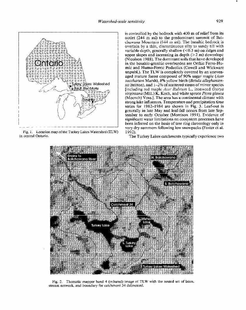
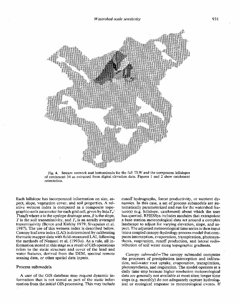
The Turkey Lakes Watershed (TLW) is an experimental watershed in the Algoma Highlands of central Ontario (Fig. 1). The TLW covers a 10.5 km2 area (Jeffries et al. 1988) and contains a headwater chain of five lakes that drains into the Batchawana River and, ultimately, Bat- chawana Bay on Lake Superior (Fig. 2). The topography

928

Watershed-scale sensitivity 929

Fig. 1. Location map of the Turkey Lakes Watershed (TLW) in central Ontario.

is controlled by the bedrock with 400 m of relief from its outlet (244 m asl) to the predominant summit of Bat- chawana Mountain (644 m asl). The basaltic bedrock is overlain by a thin, discontinuous silty to sandy till with variable depth, generally shallow (~0.5 m) on ridges and upper slopes and increasing in depth (>2 m) downslope (Nicolson 1988). The dominant soils that have developed in the basaltic-granitic overburden are Orthic Ferro-Hu- mic and Humo-Ferric Podzolics (Cowell and Wickware unpubl.). The TLW is completely covered by an uneven- aged mature forest composed of 90% sugar maple (Acer saccharum Marsh), 8% yellow birch (Betula alleghanien- sis Britton), and l-2% of scattered stems of minor species [including red maple Acer Rubrum L., ironweed Ostrya virginiana (Mill.) K. Koch, and white spruce Picea glauca (Moench) Voss.]. The area has a continental climate with strong lake influences. Temperature and precipitation time series for 1982-1984 are shown in Fig. 3. Leaf-out is generally in late May and leaf-fall occurs from late Sep- tember to early October (Morrison 1991). Evidence of significant water limitations on ecosystem processes have been inferred on the basis of tree ring chronology only in very dry summers following low snowpacks (Foster et al. 1992).

The Turkey Lakes catchments typically experience two

Fig. 2. Thematic mapper band 4 (infrared) image of TLW with the nested set of lakes, stream network, and boundary for catchment 34 delineated.

930 Band et al.

Weeklv Mean Dailv Temperatures 3 1

YI.AR/(YEARDAY)

Dailv Temperature Adiustment __

YEAR/(YEARDAY)

Weeklv Total Precipitation

YEAR(YEARDAY)

Weeklv Total Precipitation Adiustment 1

1632 (W im 1993 (65) i6j51 lh4 @iOI i~dool 19’85

YEARI(YEARDAY)

Fig. 3. Daily meteorological data for Turkey Lakes aggregated to weekly averages for 198 2- 1984: a-weekly mean daily minimum and maximum temperatures; b-weekly total precipitation; c-daily temperature adjustments for Clim change scenario; d-weekly total precipitation adjustments for Clim change scenario. Year-days are from 1 January 1982.

seasonal hydrograph rises: first, from snowmelt in late winter and early spring; second, in autumn as precipitation increases and evapotranspiration decreases, but before freezeup. For this study, a 66-ha gauged subwa- tershed (catchment 34, Fig. 4) was selected to illustrate the simulation and watershed system response to potential climate change.

Description of RHESSys

RHESSys has been described elsewhere (Band et al. 1993; Nemani et al. 1993b). Here we describe recent in- novations in the GIS analysis and representation of the landscape and the process modules. RHESSys is an integrated data and simulation package designed with a modular approach so that different landscape structures with different dominant biophysical processes can be ac- commodated. Figure 5 shows the basic structure of RHESSys, incorporating GIS data-processing modules to transform a range of spatial image and map data into a landscape (landform) description, and a set of process submodels to compute energy, water, carbon, and nutrient flux through a nested watershed system. A range of biophysical state and flux variables predicted by the model are either directly useful or can be used to diagnose both the temporal and spatial accuracy of computations. An intelligent graphical user interface is used to access and process information about watershed features and to operate the simulation modules (Mackay et al. 1994).

First, we adapt a spatial model of a watershed as a hierarchy of nested subcatchments connected by a drainage network. The drainage network is composed of stream links, the unbranched reaches of stream channels between junctions or a junction and a source. The drainage network can also contain wetlands and open-water bodies that may have multiple inlet streams but typically one outlet stream. The terrestrial portion of the subcatchments can be partitioned into a set of areas contributing drainage into each side of a stream link, the source area of a first-order tributary, or an unbroken reach of shore- line (without a defined tributary stream). Figure 4 shows this watershed description for catchment 34. This structure can be automatically extracted from a grid digital elevation model (DEM) and remotely sensed data following Mackay and Band (unpubl.). Briefly, lakes and wetlands are first identified as flat contiguous regions of the DEM. The full drainage network and associated hillslopes (including hillslopes draining into the flat areas) are then identified with an algorithm modified from Band (1989) and Lammers and Band (1990). The flat bottomland areas are determined to be open water or vegetated using spectral remote sensing information.

Each identified contiguous region is labeled as a sep- arate feature that can be explicitly incorporated into the drainage system. Using GIS overlay and processing, we retrieve all pertinent variables and store them with each land unit. Each stream link has information on length, slope, and any available channel geometry information.


Fig. 4. Stream network and bottomlands for the full TLW and the component hillslopes of catchment 34 as extracted from digital elevation data. Figures 1 and 2 show catchment orientation.

Each hillslopc has incorporated information on size, as- pect, slope, vegetation cover, and soil properties. A relative wetness index is computed as a composite topographic-soils parameter for each grid cell, given by ln(aT,l Ttanp) where a is the upslope drainage area, p is the slope, T is the soil transmissivity, and T, is an areally averaged transmissivity (Beven and Kirkby 1979; Sivapalan et al. 1987). The use of this wetness index is described below. Canopy leaf area index (LAI) is determined by calibrating thematic mapper data with field-measured LAI, following the methods of Nemani et al. (1993a). As a rule, all information stored at this stage as a result of GIS operations refers to the static structure and cover of the land and water features, derived from the DEM, spectral remote sensing data, or other spatial data inputs.

Process submodels

A user of the GIS database may request dynamic information that is not stored as part of the static information from the initial GIS processing. This may include

runoff hydrographs, forest productivity, or nutrient dy- namics. In this case, a set of process submodels are automatically parameterized and run for the watershed feature(s) (e.g. hillslope, catchment) about which the user has queried. RHESSys includes modules that extrapolate a base station meteorological data set around a complex landscape to adjust for varying elevation, slope, and as- pect. The adjusted meteorological time series is then input into a coupled canopy-hydrology process model that computes interception, evaporation, transpiration, photosynthesis, respiration, runoff production, and lateral redistribution of soil water along topographic gradients.

Canopy submodel-The canopy submodel computes the processes of precipitation interception and infiltration, soil-water root uptake, evaporation, transpiration, photosynthesis, and respiration. The model operates at a daily time step because higher resolution meteorological data are generally not available at most sites; longer time steps (e.g. monthly) do not adequately capture hydrological or ecological response to meteorological events. If

932 Band et al.

Regional Hydro-Ecological Simulation System

. _------_ _----- -- -_._ _ _. .._ ..-- -..- _ - Spatial Data Processing System

I + I LeafL@tr$dex --_---

Land Unit Extractlon ___-- Hydraulk Conduclktty

Rooting Depth

I

Extract land units wlth low withln4and unit varlance and hlgh between-land unlt variance

I ------ .- - .-- J

----------- L ~“C&Clil ‘)

-A

Slte.lNI File

Fig. 5. RHESSys flow diagram showing input data, GIS processing, model land unit (hillslope) parameterization, process submodels, and final output variables.

radiation data are available they are directly incorporated as part of the base station data set. In most cases where radiation data are not measured, they are estimated with methods adapted from Bristow and Campbell (1984). Av- erage daily absorbed radiation (Qabs) is computed as an exponential function of LA1 and incident radiation:

e abs = Qinca [ 1 .O - exp( - b LAI)].

Qinc is the incident solar radiation, a the canopy albedo, and b an extinction coefficient. An average canopy conductance is estimated on the basis of canopy LAI, incident radiation, air temperature, and vapor pressure deficit and leaf-water potential. The leaf-water potential is modeled

as a function of the soil-water potential in the root zone. Transpiration (2) is estimated with the Penman-Mon- teith equation (Monteith 1965):

R, is the net radiation, A the slope of the saturation vapor pressure-temperature curve, pa the density of the air, p,,, the density of water, X the latent heat of vaporization, cp the air heat capacity, y the psychrometric constant, VPD


the vapor pressure deficit, g, the aerodynamic conductance, and g, the canopy conductance.

Canopy gross photosynthesis uses the approach of Lo- hammer et al. (1980):

GPSN _ AC% cgcgm - . (3) gc + grill . ,

AC02 is the CO, diffusion gradient from leaf to air, c a C02/H20 diffusion correction, and g, the mesophyll conductance. Maintenance respiration is computed as a function of respiring biomass and temperature. More details of the process computations are given by Running and Coughlan (1988) and Band et al. (1993). Flux processes are considered only as one-dimensional (vertical) in the canopy submodel, with no lateral flux.

Incorporating distributed hydrology and surface hetero- geneity-To account for landscape variability of canopy, soil, and topographic features that are significant to canopy processes and to simulate lateral transfer of soil water and runoff, the canopy submodel is coupled with an approach to redistribute soil water and compute runoff production over the landscape following TOPMODEL (Be- ven and Kirkby 1979; Band et al. 1993). TOPMODEL represents soil water with saturated and unsaturated storage zones. The description here follows that of Sivapalan et al. (1987). The distribution of the saturated soil store is quantified as the depth to the saturated zone and spatially distributed over the terrain with the use of the wetness index:

Zi = (2) + l/f X - In [ (&)]- C4)

X is the areal average value of the wetness index Zi the local depth to the saturated zone. The parameter f de- scribes the exponential decay of the saturated hydraulic conductivity with depth in the soil, but is generally set by calibration. The average depth to saturation, <z>, is updated each time step on the basis of hillslope-wide water balance. Saturation runoff from each of the wetness index strata occurs when Zi 5 0 (higher values of the wetness index). Base flow, qb, from the catchment or hillslope is computed as

& qb = f exp( - X)exp( -fi) (5)

where KO is the saturated hydraulic conductivity of the soil at the surface.

The canopy submodel, including infiltration and root extraction, is run separately over each wetness index interval. This allows the simulation of drier and wetter parts of the landscape in parallel, with interaction between zones feeding back through the lateral redistribution of saturated-zone soil water. Areally weighted values of average water flux for each hillslope (runoff, baseflow, evapotranspiration, and infiltration recharge) computed over the wetness index distribution are used to update the areal average saturation deficit for each time step. In this re-

spect, the canopy processes are integrated over a time- dependent distribution function of available soil water as computed by the coupled model. The shape of the distribution depends on the landscape patterns of topography, soil, and canopy conditions, as well as the landscape average soil-water conditions. The distribution is narrow under very dry or wet conditions, in which case the canopy submodel may predict similar flux values over the entire catchment (depending on other variations of canopy and topographic conditions). Soil-water status has the most variance at intermediate landscape wetness, which leads to the computation of more spatially hetero- geneous flux values. Accounting for lateral water redistribution and differential available water and canopy properties in this manner can have significant impact on landscape average carbon and water flux (Band et al. 1993; Band 1993), especially in the intermediate landscape wetness state.

Because meteorological conditions, canopy cover, and soils may not be stationary across hillslopes of different exposure, the integrated model is run separately for each hillslope comprising the watershed as shown in Fig. 4. Therefore, the model execution is hierarchically nested as watershed-hillslope-wetness index with the actual processes simulated at the hillslope-to-wetness index scale and aggregated and reported by hillslope and then reported for the full watershed. Each flux or storage computed by the model could also be mapped back to the wetness index interval level within each hillslope. In the current application, however, we report watershed aggregated values.

Model calibration and diagnosis

Model parameters for the TOPMODEL modules are calibrated to observed daily runoff. Two parameters for TOPMODEL, f and &, were calibrated with a simplex method using simulated and observed daily runoff data for catchment 34 for a 2-yr test period. Figure 6 shows the correspondence of observed and simulated daily runoff for the 3-yr period from 1 January 1982 through 1984. Some lack of fit is due to variability in precipitation between the meteorological station and catchment 34 (on opposite sides of Batchawana Mountain), which we have not attempted to adjust, and also to the daily time step that does not resolve storm intensity. In addition, precipitation is set as snow or rain based on mean daily temperature, which causes some error around daily mean temperatures of 0°C. Rather than attempting to adjust these instances for a better fit, we simply recognize the limitations of these simulations with available meteorological data.

As a further check of the simulation system’s consistency and performance we have compared observed and predicted values of state and flux variables including long- term forest stand biomass accumulation and snow de- pletion curves for areas of the TLW (Band 1994) and have found reasonable agreement. Note that these variables are not used as part of the calibration, so their

934 Band et al.

1982 W) (W 1270) 1993 (W (545) (635) 1994 WOI WO) WW 1995

YEAR/(YEARDAY)

Weekly Total Deviation From Control Outflow

I

I I ---

1992 w WI (270) 1993 (455) w4 18351 1994 WO) (W ww 1995

YEARJYEARDAY)

Weekly Total Deviation From Control Outflow

1982 60 (IW (270) 1993 ww (W (835) 1984 ww wol ww 1995

YEARQYEARDAY)

Fig. 6. Observed and simulated (control) daily runoff (aggregated to total weekly values) for catchment 34 (top), and deviations from the control for the three climate change scenarios (middle and bottom). Year-days are from 1 January 1982.

correspondence with observations is indicative of the model’s internal consistency.

Simulation of watershed hydroecological processes under changed climate

Because RHESSys responds directly to daily meteorological data, the impact of potential climate change can be evaluated by substituting appropriate time series reflecting different scenarios. To an extent this can be done by using historical data for particularly warm and dry years, wet and cold years, etc. However, these data will only show effects of changing distributions of temperature, precipitation, humidity, and radiation. A major effect of greenhouse gas-induced climate change may be a significant adjustment of physiological stomata1 and photosynthetic processes to increased atmospheric CO2 concentrations (Mooney et al. 199 1; Schindler and Bayley 1993).

We used an experimental design for investigating change scenarios similar to that of Running and Nemani (199 1) by simulating the effects of climatic change in three suc- cessive steps: first, adjusting the daily meteorological record with seasonal shifts in temperature and precipitation (Table 1) (the “Clim” scenario in the simulations below); second, a model parameterization to incorporate the physiological response of the canopy to elevated atmospheric CO2 concentrations is added to the Clim scenario (Clim+Phys); third, potential increases in forest cover due to increased temperature, growing season length, and CO2 fertilization are added by increasing LA1 (Clim+ Phys + LAI).

Approximate shifts in seasonal temperature and precipitation are taken from the Intergovernment Panel on Climate Change (IPCC, Mitchell et al. 1990) as a standard reference for comparison with other studies. Figure 3 shows the weekly aggregated temperature and precipitation records for Turkey Lakes for 1982-1984 and the stepwise changes made in the above simulations compared to the control run. Year-day is recorded from 1

Table 1. Stepwise changes in simulation conditions. Winter months- DJF, spring months- MAM; summer months-JJA; autumn months-SON.

Change scenario Climate changes DJF MAM JJA SON

Climate* Temp. (“C) +4.0 +3.5 +3.0 +3.5 Precip. (O/o) +10 0 -10 0

Physiologyt Physiol. response Canopy conductance Mesophyll conductance to CO, doubling Hz0 (ms-I) CO, (ms-l)

LA1

Conductance (%)

Forest cover changes

-30

Growing season

+30

Winter

Leaf area index (%) +30 0

* Source, Houghton et al. 1990. t Source, Running and Nemani 199 1.


January 1982. The physiological response of stomata1 conductance to a doubling of ambient COZ concentration is approximated by decreasing the maximum canopy conductance by 30% and increasing the mesophyll conductance by 30% in the second and third steps following Cure and Acock (1986) and Running and Nemani (199 1). The 30% increase in LA1 is an arbitrary value and is chosen simply to illustrate the direction of change brought about by potential enhanced growth of the forest canopy in response to atmospheric change (both warming and CO, change).

Simulation results

A control simulation for observed conditions between 198 1 and 1984 is first run to generate baseline time series for catchment-aggregated daily runoff volume, evapotranspiration, net canopy photosynthesis, saturation depth in the soil (as used in TOPMODEL, above), and snowpack water equivalent. Deviations from these control runs for each of the above scenarios are then examined to determine the relative impacts on watershed 34 aggregated hydroecological processes. We present the results of the 1982-1984 period (1981 is considered an initial- ization year), which contain a good range of meteorological conditions. The 1982-1983 water-year (1 October 1982-30 September 1983) was one of the warmest and driest years on record in the TLW, whereas the preceding and following years were more normal to wetter.

Snowpack-The shift in temperature and precipitation patterns in the Clim run results in major changes in the magnitude and timing of snowpack accumulation and snowmelt. Figure 7 shows control snowpack water equivalents and the deviations from the control for the Clim scenarios. The reductions in snowpack compared to the control results from reduced snowfall (increased winter rainfall) and an earlier snowmelt brought about by higher temperatures. There are no direct effects of increased CO2 concentrations on the snowpack, and the increased LA1 scenario has little influence because the area is domi- nantly deciduous.

Evapotranspiration -Summer evapotranspiration (ET) rates with the Clim shifts increase through all growing seasons compared to the control (Fig. 8) with the excep- tion of short periods of relative decreases in the dry summer of 1983 (between year-day 800 and 1,000). In the Clim+Phys run, this effect is reversed because ET declines through summer following the parameterized sto- matal response to increased COZ concentrations; however, these summer reductions are partially offset by the increased length of the growing season, such that spring and fall ET rates are still higher than the control rates. Finally, increasing LA1 by 30% results in summer ET rates closer to the control than is achieved with the Clim+Phys model runs, whereas fall and spring rates approach the former two runs.

YEAR/(YEARDAY)

Weekly Total Deviation From Control Snowpack

-7 7

I I I I I I I I I I I , I 1

1992 W) (W (270) 1993 (455) 6-w w-35) 1994 wm FJW ww 1995

YEAR/(YEARDAY)

Fig. 7. Simulated control snowpack water equivalents (aggregated to mean weekly values) for 1982-1984 and deviations to the control for the Clim scenario.

Net canopy photosynthesis (PSN) -In the Clim scenario the decrease in snowpack depth and duration, coupled with reduced precipitation and increased temperatures in summer, results in an increase in water stress and con- sequent reduction in canopy carbon assimilation (Fig. 9) similar to changes in ET. Seasonal changes in the net carbon flux show an increase after the earlier snowmelt and warmer spring temperatures, followed by summer reduction due to water stress. The Clim+Phys adjustment leads to an increase of carbon assimilation through- out the growing season compared with the control except in the very dry 1983 summer. The Clim + Phys reduction in summer net canopy photosynthesis (PSN) however, is minor compared to the large drop in the Clim run. The final addition of a 30% LA1 increase leads to the greatest increase in carbon assimilation early in each growing season due to increased radiation absorption and canopy conductance and intermediate changes relative to the control due to water stress late in the summer.

Band et al.

1982 Pw (W i270) 1963 (455) (5W (035) 1964 ww WO) WW 1965

YEAR/(YEARDAY)

Weekly Total Deviation From Control Evapotranspiration

I I I I I I I I I I I I ’ 1962 WJ) WJI (2701 1983 (455) wx 6351 1964 WO) l910) W-W 1965

YEAR/(YEAFiDAY)

Fig. 8. Simulated control evapotranspiration (aggregated to total weekly values) for 1982-1984 and deviations from the control for the three different climate change scenarios.

Runocffproduction -The changes in snowpack dynam- ics and evapotranspiration are reflected in the patterns of watershed runoff (Fig. 6, middle panel). Clim model runs show a shift in the snowmelt hydrograph resulting in an earlier rise and fall in runoff that dominates the plot of discharge deviations. The lower panel of Fig. 6 shows more detail of the deviations away from the snowmelt period. For the Clim run, summer baseflow is generally lower and more extended in duration as soil water from the earlier snowmelt is depleted, requiring a greater recharge of soil water in autumn before significant increases of runoff can occur. The Clim+Phys results in increased summer baseflow reflecting the reduction in transpiration. Augmenting the canopy LA1 causes an intermediate response with more moderate declines in baseflow in all years relative to the Clim scenario, because the additional LA1 offsets the changes in stomata1 physiology compared to Clim+Phys. This latter effect is partially due to increased canopy interception of summer precipitation with the higher LA1 and the relative increase of canopy conductance compared to the Clim+Phys run.

1962 W (~W 12701 1963 (455) (W (535) 1964 I=Ql WOI (1cw 196!

YEAR/(YEARDAY)

Weekly Total Deviation From Control Net Photosynthesis

1982 (WI uw (2701 1963 (455) (5451 (6351 1964 WJ) wol ww 1965

YEARQYEARDAY)

Fig. 9. Simulated control net canopy photosynthesis (aggregated to total weekly values) for 1982-l 984 and deviations from the control for the three different climate change scenarios.

Summary of annual changes-Figure 10 shows the annual changes in the above variables relative to the control, along with saturation store-water deficit (relative to full profile saturation) and canopy respiration for 1982 (wet year) and 1983 (dry year). An interesting difference between the wet and dry years is the net change in outflow, which represents a balance between increased winter runoff (increased precipitation and higher temperatures) and potential decreases in summer flow (higher ET). This in- dicates that the impact of potential climate changes can qualitatively shift from year to year in terms of hydrologic flux. Although the simulated long-term average outflow (estimated from the average change in a lo-yr simulation period) decreases for the Clim changes and increases with the Clim+Phys changes, the nonlinear and potentially offsetting effects of meteorological conditions and physiological processes on daily and seasonal water flux can cause divergent response to climate change in different years. The conservation of water brought about by greater stomata1 resistance in summer is offset by the earlier thaw and later freeze, such that climate change effects are sen-


Percent Change in Response For 1982 70

60

50

40

30

20

10

0

-10

-20

SZD ET OUTFLOW PSN RESP

Percent Change in Response For 1983 70

60

50

40

30

20

IO

0

-10

-20

SZD ET OUTFLOW PSN RESP

Fig. 10. Annual deviations of the three climate change scenarios from the control simulation for different hydrological and ecological flux processes. Average watershed soil saturation zone deficit (below full profile saturation)-SZD; average canopy maintenance respiration- RESP. Numbers above the bars for PSN and RESP are the annual totals in g C m-2.

sitive to both the magnitude and timing of weather conditions. For the TLW, it seems that normal to wet years ( 1982 and 1984) may show increased outflow as more precipitation falls in the dormant winter period and less in the growing season. This increase is maximized in the Clim+Phys scenario with greater stomata1 resistance but no increase in leaf area. In the warm-dry years, this effect is reversed by offsetting increases in summer ET, even for the Clim+Phys scenario. Finally, PSN shows consistent reductions in all years for the Clim runs, but consistent increases in the latter two runs that incorporate stomata1 adjustment to CO2 concentration.

Discussion

The changes in meteorological data, canopy physiological processes, and forest cover prescribed above rep- resent reasonable, but incomplete change scenarios for

evaluating the effects of climate change on watershed processes. Although each numerical experiment was operated as a step change in simulation conditions, a transient response to gradual change may involve other biophysical adjustments and feedback that we cannot account for. Nevertheless, the changes in simulation conditions are consistent with standard approaches to climate change assessment, and the range of scenarios we have investi- gated with a distributed watershed model is more com- prehensive than many evaluations of 2 x CO2 atmospheric concentration evaluations that may not incorporate ecosystem physiological response or a distributed approach. Each of the set of model prescriptions results in a distinct system behavior, and we expect that additional feedback we could incorporate would further add to the variance of results.

With all three prescribed changes to simulation conditions, the model results suggest that in this portion of North America watershed response that is not currently water limited is unlikely to become significantly more water limited in a warmer, CO,-enriched climate. Changes in evapotranspiration, forest productivity, and runoff production simulated by considering only temperature and precipitation changes are moderated or reversed when stomata1 response to CO2 enrichment is considered. The tendency for some increases in summer water stress is not sufficient to offset the enhanced productivity brought about by the longer growing season, reduced temperature limitations, and higher photosynthetic rates.

The model runs indicate that there exists a series of potentially offsetting effects of climate change on runoff production and other watershed processes. Comparing different control years suggests the qualitative response of different processes (e.g. increase or decrease) to climate change will vary in accordance with the relative changes in these offsetting processes that appear to shift with normal interannual weather conditions. This may indicate that long-term average changes in specific hydrologic processes may be more resilient to climate change than pre- viously expected, although carbon assimilation by the canopy in TLW showed consistent year-to-year increases.

We are still quite uncertain about the interaction of biophysical processes active in the watershed at both short and long time scales, so that the simulations run here may be significantly biased. Future work should extend our ability to simulate long-term response of the watershed to gradual change, rather than prescribing step changes to present conditions. This will require incorporation of a more physiologically based method to compute sto- matal conductance under conditions of increasing COZ concentrations, as well as methods to better account for nitrogen and other nutrient limitations. Some method of assessing changing probabilities of large-scale disturbance in the watershed, particularly of fire ignition and spread, would be very desirable.

Here, we have reported only the aggregated catchment response in a single headwater catchment. An important advantage of RHESSys is the ability to simulate and report results for multiple, nested catchments, and the spatial variablity of response within each catchment. This

938 Band et al.

ability is an important asset in testing and diagnosing model performance and is being continued for the Turkey Lakes and other watersheds.

References

BAND, L. E. 1989. A terrain based watershed information system. Hydrol. Processes 3: 15 l-l 62.

- 1993. Effect of land surface representation on forest water and carbon budgets. J. Hydrol. 150: 749-772. . 1994. Development of a landscape ecological model for management on Ontario forests: Phase 2-extension over an east/west gradient over the province. Ont. For. Res. Inst. Ont. Min. Nat. Resour. Rep. 17.

-, P. PATTERSON, R. NEMANI, AND S. W. RUNNING. 1993. Forest ecosystem processes at the watershed scale: Incor- porating hillslope hydrology. Agric. For. Meteorol. 63: 93- 126.

-, AND OTHERS. 199 1. Forest ecosystem processes at the watershed scale: Basis for distributed simulation. Ecol. Model. 56: 171-196.

MACKAY, D. S., V. B. ROBINSON, AND L. E. BAND. 1994. A knowledge-based approach to the management of geo- graphic information systems for simulation of forested ecosystems, p. 5 1 l-534. In W. K. Michener et al. [eds.], En- vironmental information management and analysis: Eco- system to global scales. Taylor and Francis.

MITCHELL, J. F. B., S. MANABE, V. MELESHKO, AND T. TOKIOKA. 1990. Equilibrium climate change and its implications for the future, p. 131-172. In J. T. Houghton et al. [eds.], Climate change. The IPCC scientific assessment. Cam- bridge.

MONTEITH, J. L. 1965. Evaporation and envrionment, p. 205- 233. In Proc. 19th Symp. Sot. Exp. Biol. Cambridge.

MOONEY, H. A., B. G. DRAKE, R. J. LUXMOORE, W. C. OECHEL, AND L. F. PITELKA. 199 1. Predicting ecosystem responses to elevated CO, concentrations. Bioscience 41: 96-104.

MORRISON, I. K. 199 1. Addition of organic matter and ele- ments to the forest floor of an old-growth Acer saccharum forest in the annual litter fall. Can. J. For. Res. 21: 462- 468.

BEVEN, K., AND M. J. KIRKBY. 1979. A physically-based, variable contributing area model of basin hydrology. Hydrol. Sci. Bull. 24: 43-69.

BRISTOW, K. L., AND G. S. CAMPBELI,. 1984. On the relation- ship between incoming solar radiation and daily maximum and minimum temperature. Agric. For. Meteorol. 31: 159- 166.

NEMANI, R., L. PIERCE, S. RUNNING, AND L. BAND. 199 3a. Forest ecosystem processes at the watershed scale: Sensi- tivity to remotely-sensed leaf area index measurements. Int. J. Remote Sensing 14: 25 19-2534.

-, S. W. RUNNING, L. E. BAND, AND D. L. PETERSON. 1993b. Regional HydroEcological Simulation System: An illustration of ecosystem models in a GIS, p. 297-304. In M. F. Goodchild et al. [eds.], Environmental modeling with GIS. Oxford.

CURE, J. D., AND B. ACOCK. 1986. Crop responses to carbon dioxide doubling: A literature survey. Agric. For. Meteorol. 38: 127-145.

NICOLSON, J. A. 1988. Water and chemical budgets for terrestrial basins at the Turkey Lakes watershed. Can. J. Fish. Aquat. Sci. 45(suppl. 1): 88-95.

FOSTER, N. W., I. K. MORRISON, X. YIN, AND P. A. ARP. 1992. Impact of soil water deficits in a mature sugar maple forest: Stand biogeochemistry. Can. J. For. Res. 22: 1753-1760.

HOUGHTON, J. T., G. J. JENKINS, AND J. J. EPHRAUMS [EDS.]. 1990. Climate change: The IPCC scientific assessment. Cambridge.

JEFFRIES, D. S., J. R. M. KELSO, ANX) I. K. MORRISON. 198 8. Physical, chemical and biological characteristics of the Tur- key Lakes watershed, central Ontario, Canada. Can. J. Fish. Aquat. Sci. 45(suppl. 1): 3-13.

LAMMERS, R. B., AND L. E. BAND. 1990. Automating object representation of drainage basins. Computers Geosci. 16: 787-8 10.

RUNNING, S. W., AND J. C. COUGHLAN. 1988. A general model of forest ecosystem processes for regional applications. 1. Hydrologic balance, canopy gas exchange and primary production processes. Ecol. Model. 42: 125-l 54.

AND R. R. NEMANI. 199 1. Regional hydrologic and caibon balance response of forests resulting from potential climate change. Clim. Change 19: 349-368.

-, AND OTHERS. 1989. Mapping regional forest evapotranspiration and photosynthesis by coupling satellite data with ecosystem simulation. Ecology 70: 1090-l 10 1.

SCHINDLER, D. W., AND S. E. BAYLEY. 1993. The biosphere as an increasing sink for atmospheric carbon: Estimates from increased nitrogen deposition. Global Biogeochem. Cycles 7: 7 17-733.

LOHAMMER, T., S. LARSSON, S. LINDER, AND S. FALK. 1980. SIVAPALAN, M., E. F. WOOD, AND K. BEVEN. 1987. On catch- FAST-simulation models of gaseous exchange in Scats ment similarity. 2. A scaled model of storm runoff pro- pine. Ecol. Bull. 32: 505-523. duction. Water Resour. Res. 23: 2266-2278.

Documents

Ecosystem processes at the watershed scale: …. Oceanogr., 41(5), 1996, 928-938 0 1996, by the American Society of Limnology and Oceanography, Inc. Ecosystem processes at the watershed