Embed Size (px)
Citation preview

Xiao-guang Zhang Research Manager Australian Productivity Commission 27 May 2014, 10:30am–12:00nn 1650S, ADB Headquarters
Seminar Series on
Regional Economic Integration
“Assessing the Economy-wide Impacts of RCI Instruments”

Background (1)
– About the Productivity Commission
• Government’s principal review and advisory body on microeconomic policy
reform and regulation
– Roles of the Commission
• Objective analysis for better informed policy decisions
• Supporting community awareness and policy debate
– Three core design features
• Independent
• Transparent
• Community-wide perspective

Background (2)
– Extensive use of quantitative tools and economic models
• Particularly, CGE models for analysing economy-wide issues
• Involved in the development of many CGE models, such as various Australian
models (CoPS), SALTER model (the origin of GTAP)

Modelling economic integration
– The degrees economic integration
• Preferential trading area
• Free trade area (NAFTA)
• Custom union
• Common market
• Economic union (EU)
• Economic and monetary union (EU/€)
• Complete economic integration

PC’s recent work related to
economic integration
– Bilateral and Regional Trade Agreements (2010)
• Review of bilateral and regional trade agreements
• Their impacts on Australian trade and economic performance
• Their impacts on reducing the barriers to the markets of Australia’s trading
partners
– Strengthening trans-Tasman Economic Relations (2012)
• Review the 30 years Australia-New Zealand Closer Economic Relations Trade
Agreement (ANZCERTA)
• Achievements so far and areas for reforms
• The ways forward to closer economic integration

A case study: trans-Tasman
economic integration – History
• Started with the Australia-New Zealand Closer Economic Relations Trade
Agreement (ANZCERTA) in 1983
• Rapid progress on economic integration after a review in 1988
• CER has been highly successful in removing explicit restrictions on trade and
substantial progress has been made on reducing other barriers to integration,
such as labour and capital movements
– Achievements
• Trade in goods largely liberalized
• Trade in services is partially liberalized
• Substantial increase in bilateral investment flows
• Free movement of people, a key feature
• Extensive inter-government cooperation

Review of 30 years of CER
– A joint study by the Productivity Commissions of Australia and New
Zealand
• Final report ―Strengthening trans-Tasman Economic relations‖ released in 2012
– Purposes
• Potential areas of further economic reform and integration
• Economic impacts and benefits of reform
• Transition and adjustment costs that could be incurred
• Identification of reform where joint net benefits are highest
• The means by which they might be best actioned
• The likely time paths over which benefits are expected to accrue

Quantifying the effects of
economic integration
– Require global CGE modelling
• A global CGE model (ANZEA), developed for this study
– The ANZEA model
• Developed on the basis of a simple global model (Zhang, 2013 GTAP
conference paper)
• Use data drawn from GTAP database (version 8)
– A simple model approach
• CGE models structurally similar and simple
• Model code can be made simple and transparent

Motivations for simple models
– Diverse policy issues
• Require different models: national/global or static/dynamic
• Each used for a wide-range of applications
– Off-the-shelf models
• Long and complex code: too many variables/equations
• Designed for multi-purposes
• Mix model theory and interpretation
• Costly to modify and adapt to new applications

An alternative modelling
approach
– The ideal approach
• A simple model structure with a simple database
• Easily adaptable to any application
– The meaning of ―simple‖
• Not a stylised ―toy‖ model
• Not with a small-sized database
• A simple structure for model equations and database
– Benefits from a simple model
• Transparent and easy to understand the theory
• Easy to change or modify to incorporate new features
• Develop application-specific models from a basic model

ANZEA model database structure (1)
– Country/region input-output tables (6 matrixes and 2 vectors)
• Purchases of domestic and imported goods by users
• Indirect tax revenues
• Basic values of non-margin exports
• Export tax revenues
• Purchases of primary factors
• Factor tax revenues
• Basic value of margin exports (vector)
• Production tax revenue (vector)
– World trade data (2 matrixes)
• Basic values of imports
• Import margins

ANZEA model database structure (2)
– Bilateral capital and investment data (2 matrixes)
• Bilateral capital stocks by industry and country
• Bilateral saving-investment flows by country

Database structure for a representative region (r)

Bilateral capital stock and saving-investment matrixes
REG(s) REG(s)
Pt_is(“inv”,s) Q k(j,r,s)
Pt_is(“inv”,s) Q
inv(r,s) REG
(r)
(Column sum = Capital used
in host region s) (Column sum = Investment
in host region s)
(Row sum =
Capital
owned
by home
region r)
(Row sum =
Savings
in home
region r)
REG
(r)
3. Capital stock matrices (j,r,s) 4. Investment matrix (r,s)

Equation structure (1)
– A system of 35 equation blocks in 4 sections
• Consumption: region and user demands for goods
• Production: industry outputs and demands for factors
• Factor supplies: factor market clearing conditions
• Income distribution: allocation of income between final users
– Note that
• Includes only core variables essential for model solution
• No reporting variables

Equation structure (2)
– Demand for imports and domestic goods (eqs.1-9)
• Three levels of demands for goods by user
• Associated purchasers’ prices derived from their basic prices
– Industrial demands for factors (eqs.10-17)
• Outputs by industry (CRTS)
• Demands for factors by industry
• Basic prices of goods (CRTS)
– Regional supplies of factors (eqs.18-24)
• Market equilibrium for factors
• Factor price equalisation for mobile factors

Equation structure (3)
– Final users’ expenditure (eqs.25-35)
• Income derivation
• Expenditure by final user
• Trade balance or saving-investment gap

Core variables and equations
– Overall 35 equation blocks
• 28 define 28 endogenous variables
• 7 specify solution conditions (eqs.18, 19, 21, 23, 32, 34 and 35)
– 7 variable blocks undefined
• 3 for factor basic prices (P f(“land”,j,r), W(r), Pk
(j,r,s))
• 1 for rate of return to home capital (R_js(r))
• 1 for bilateral investment flows (V inv(r,s))
• 1 for world expected rate of return (Re_rs)
• 1 for net foreign investment inflows (YNFI(r))
– Undefined variables solved from solution conditions
• Market Clearing Conditions (MCC)
• Price Equalisation Conditions (PEC)

Undefined variables and MCC/PEC equations
Undefined variables
MCC/PEC equations
P f(“land”,j,r) Basic price of land Eq.18 MCC for sectoral land Q f(“land”,j,r)
W(r) Basic price of labour Eq.19 MCC for regional labour X lab( r)
R_js(r) Rate of return to home capital Eq.21 MCC for home capital X k(r)
Pk(j,r,s) Basic price of capital Eq.23 PEC for rates of return to
capital R(j,r,s)
Re_rs
World expected rate of return Eq.32 MCC for global savings r V
sav(r)
V inv(r,s)
Bilateral investment flows Eq.34 PEC for expected rates of
return to investment Re (r,s)
YNFI(r) Net foreign investment Eq.35 MCC for host real investment i Q_s(i,“inv”,r)

Applications to regional
economic integration
– A case study: Australia-New Zealand close economic relations
– 5 scenarios analysed
1. Eliminating Australian and New Zealand tariffs on imports from all sources;
2. Productivity improvements in Australia and New Zealand;
3. Economic expansion in Asia;
4. Migration from New Zealand to Australia;
5. Liberalising trade in services via commercial presence (by reducing barriers to
trans-Tasman FDI in services)

1. Removing most-favoured-
nation (MFN) tariffs – Shocks
• Reduce Australia and New Zealand MFN tariffs on all imports to zero
– Gains from
• More efficient allocation of resources from protected sectors to more competitive
sectors
• Seme inputs and more outputs
– Results
• GDP 0.3% in AU and 0.4% in NZ
• Output and export in mining, food prods and services and in TCF and motor
vehicle and parts

2. Productivity improvements in
Australia and New Zealand (1)
– Shocks
• An improvement in productivity (specifically, factor augmenting technical
change) of 1 percent for all factor inputs in each economy
•
– Transmission mechanisms
• competitiveness and output of country A and output of B;
• factor income in A and import demand from B, output in B;
• factor income in A leads to mobile factor move from B and output of B.
– The results: 1% productivity improvement in New Zealand
• NZ GDP 1.37%, AU GDP -0.01%
• AU export – 0.09%: to NZ 1%, to others -0.15%
• AU import 0.09%

2. Productivity improvements in
Australia and New Zealand (2)
– The results: 1% productivity improvement in Australia
• AU GDP 1.31%, NZ GDP -0.09%
• NZ export – 0.32%: to NZ 0.38%, to others -0.5%
• AU import 0.22%
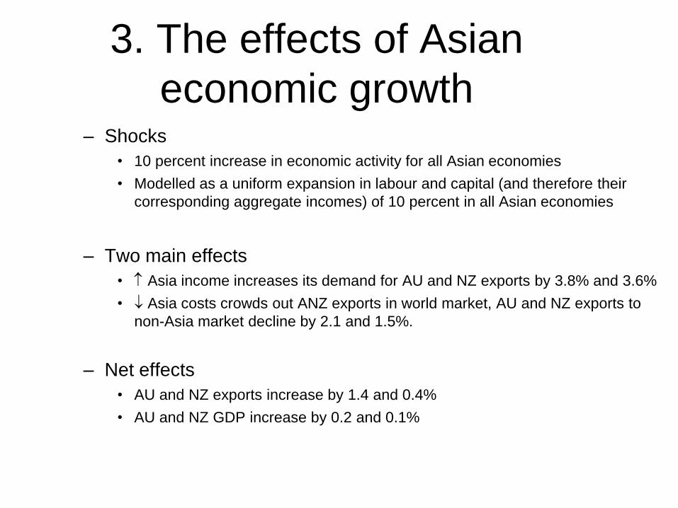
3. The effects of Asian
economic growth – Shocks
• 10 percent increase in economic activity for all Asian economies
• Modelled as a uniform expansion in labour and capital (and therefore their
corresponding aggregate incomes) of 10 percent in all Asian economies
– Two main effects
• Asia income increases its demand for AU and NZ exports by 3.8% and 3.6%
• Asia costs crowds out ANZ exports in world market, AU and NZ exports to
non-Asia market decline by 2.1 and 1.5%.
– Net effects
• AU and NZ exports increase by 1.4 and 0.4%
• AU and NZ GDP increase by 0.2 and 0.1%

4. Trans-Tasman migration
– Shocks and assumptions
• 1 percent increase in the supply of New Zealand labour in Australia (about 3000
workers)
• Keep capital fixed in AU and NZ
– Motivation of migration
• Expected wage differential net of migration costs
• Migration reduce wage differentials and increase total output
– Results
• Employment 0.02% in AU and 0.14% NZ
• GNI 0.01% in AU and 0.08% NZ
• GNI per worker 0.01% in AU and 0.06% NZ

5. Reducing barriers to commercial
presence in services (1)
– Shocks
• Empirical estimates of barriers to foreign investment in service industries
(CIE 2010)
• Adjustments for the project: cost-escalating and rent-creating barriers
– Scenarios
• A reduction in trans-Tasman barriers to FDI in all services industries (except the
banking sector)
• A reduction in trans-Tasman barriers to FDI in communications industries
• A reduction in the barriers to FDI in communications industries irrespective of
where the FDI originates

5. Reducing barriers to commercial
presence in services (2)
– Results
• Preferential barriers to services
• Preferential barriers to Communications
• Non-preferential barriers to Communications

Effects on GDP and GNI of eliminating barriers to commercial
presence
Australia New Zealand
% changes % changes
GDP
Preferential
Remove trans-Tasman barriers to FDI — all services -0.01 0.13
Remove trans-Tasman barriers to FDI — communications – 0.01
Non-preferential
Remove barriers to FDI all countries — communications 0.11 0.22
GNI
Preferential
Remove trans-Tasman barriers to FDI — all services – 0.07
Remove trans-Tasman barriers to FDI — communications – 0.01
Non-preferential
Remove barriers to FDI all countries — communications 0.06 0.10

Sensitivity analysis: closure settings
– Sensitivity to closure settings: test assumptions about capital
mobility
• C1: K stock fixed in host countries
• C2: K stock fixed in home countries, mobile across host countries
• C3: Variable global K, fixed investment/capital ratio
• C4: Variable global K stock, fixed rates of return
– Sensitivity to parameter values
• Amington substitution
• Factor substitution
• Capital substitution
•
– Importance of the ―range‖

Concluding remarks
– CGE models are suitable for a wide range of policy options for
regional economic integration
– A simple model structure is adaptable to many applications of
regional integration

Xiao-guang Zhang
Productivity Commission, Australia
Seminar, OREI, ADB, May 27, 2014, Manila
Infrastructure reform and income distribution:
A case study of Australia

Outline
– Back ground
• The 1990 Structural changes in Australian infrastructure industries in the 1990s
• Effects on production and consumption
– Analytical framework: a two-model approach
• A regional CGE model of the Australian economy
• A micro-simulation model based in the household expenditure survey data
– An example of the results: electricity industry
• CGE results
• Micro-simulation results

Modelling income distribution impacts
– ―Distributional effects of changes in Australian infrastructure
industries during the 1990s‖, with G. Verikios, Staff Working Paper,
2008, Productivity Commission.
– Infrastructural industries
• Electricity
• Gas
• Ports and rall freight
• Telecommunications
• Urban transport
• Water and sewerage

Back ground (1)
– During the 1990s, many changes occurred in these industries
• Management structure
• Ownership structure
• Taxation treatment
• Technology and management practices
– Expected effects on production
• Costs, prices
• Productivity
• Outputs, employment
• Factor income

Back ground (2)
– Expected effects on households
• Household nominal income
• Household expenditure
• Household real income

Aim of the study
– Focus on
• The effects on the distribution of real income between households at the
regional level

Analytical framework: a two-
model approach
– A regional CGE model of the Australian economy (MMRF)
• 8 states/territories
• Each has one aggregate household
• 54 goods/industries
• 8 labour occupations
• Early 1990s data
– A micro-simulation model based on the household expenditure
survey data (ID model)
• the 1993-94 Household Expenditure Survey (HES)
• Expenditure data: goods and services > 700
• Income source data: 8 labour occupations, many non-labour incomes and
income tax, transfer payments
• Sample size > 8000 households

MMRF-ID framework
Changes in infrastructure
prices and inputs
MMRF
Changes in goods and factor prices by
region
HESa ID
Changes in household
nominal income Changes in HCPIb
Changes in real household
income
Model inputs or
outputs
KEY
Model

Use of the MMRF-ID framework
– Changes in an infrastructure industry are introduced in the MMRF
model to simulate the effects on
• Goods prices
• Factor prices
– The CGE effects are used to shock the equivalent variables in the
ID model to derive changes in each household’s
• Nominal income: factor price index
• Nominal expenditure: household CPI of HCPI
• => Change in household real income = change in household factor price index -
change in HCPI
• Compare changes in real income distribution

Linking the micro-sim model to
the CGE model
– Linking household income sources with MMRF factor incomes
– Linking household expenditure items with MMRF consumption
goods

Sources of household income
in MMRF and ID MMRF model ID model (as defined in HES)
Wages for eight occupations (same as those in ID)
Wages for Managers and administrators; Professionals; Para-Professionals; Tradespersons; Clerks; Salespersons and personal service workers; Plant and machine operators and drivers; Labourers and related workers
Non-labour (capital and land) private income sources
Interest; Investment; Property rent; Superannuation; Business; Workers compensation; Accident compensation; Maintenance; Other regular sources; Private scholarship; Government scholarship; Overseas pensions
Unemployment benefits (Commonwealth) Unemployment benefits
Other government benefits (Commonwealth and State)
Sickness benefits; Family allowance; Veterans’ pensions; Age pensions; Widows’ pensions; Disabled pensions; Supporting parenting benefits; Wives’ pensions; Other Australian government benefits; AUSTUDY support; Carers’ pensions; Other overseas government benefits
Direct taxes Direct taxes

Important features of the ID
database
– Household expenditure patterns
– Household income source patterns
– Provide a simple but powerful basis for result interpretation: why a
set of the same price changes could lead to a diverse changes in
household incomes.

Composition of gross income
and direct taxes by decile (%)
Income decile Labour
income Non-labour income
Government benefits
Direct taxes
Lowest 32.7 -9.1 76.4 3.0
Second 41.7 9.9 48.5 6.0
Third 33.8 14.2 52.0 6.4
Fourth 50.1 10.9 39.0 9.3
Fifth 63.3 18.1 18.6 14.0
Sixth 73.7 15.6 10.7 16.5
Seventh 77.1 15.8 7.1 18.5
Eighth 84.2 13.3 2.5 20.2
Ninth 86.3 12.6 1.2 22.5
Highest 80.2 19.5 0.3 29.1

Shares of occupational wages
in labour income by decile (%)
Occupation 1st 2nd 3rd 4th 5th 6th 7th 8th 9th 10th
Managers & administrators 14.2 8.0 10.8 10.0 10.7 9.6 12.2 13.1 14.4 25.7
Professionals 8.2 9.9 13.1 11.8 12.8 14.3 15.8 15.8 19.4 33.1
Para-professionals 6.8 9.9 8.0 5.5 12.6 7.9 8.1 9.4 9.0 8.9
Tradespersons 11.9 19.5 19.8 18.6 20.3 16.7 12.6 14.3 12.7 6.0
Clerks 9.8 10.5 16.1 14.2 14.2 15.0 19.0 17.2 18.2 12.4
Salespersons & personal service workers 13.8 12.5 12.7 13.2 9.8 13.0 12.1 12.1 11.7 6.9
Plant & machine operators, & drivers 12.8 9.8 5.0 9.7 5.6 10.0 7.7 8.4 7.6 4.7
Labourers & related workers 22.4 19.8 14.7 17.0 13.9 13.4 12.6 9.7 7.0 2.3

Shares of infrastructure services and
capital expenditure in total household
expenditure (%)
Income decile Electricity Gas Ports & rail
freight Telecomm-unications
Urban transport
Water & sewerage
Capital spending
Lowest 2.4 0.7 0.4 2.6 1.0 0.8 9.9
Second 2.3 0.6 0.3 2.3 1.0 0.9 12.9
Third 2.4 0.7 0.4 2.6 1.2 1.1 11.2
Fourth 2.0 0.6 0.3 2.3 1.0 1.0 18.8
Fifth 1.7 0.5 0.3 1.9 0.9 0.9 21.9
Sixth 1.5 0.5 0.4 1.7 0.8 0.8 24.8
Seventh 1.4 0.5 0.5 1.6 0.8 0.7 26.7
Eighth 1.2 0.4 0.5 1.4 1.1 0.6 29.9
Ninth 1.1 0.4 0.5 1.3 0.9 0.6 35.4
Highest 0.8 0.3 0.3 1.0 0.6 0.5 44.1
Average 1.5 0.4 0.4 1.7 0.9 0.7 27.7

Interpretation of the results
– Economy-wide results (CGE model)
• Mechanism of transmission from shocks to final changes in goods and factor
prices
• Can be explained by CGE model’s theoretical structure
• First round effects: labour productivity in an infr-ind. its price and
output the costs and outputs of downstream inds.
• employ in the infr-ind. its wage and returns to other factors
• Second-round effects: household income demands for all goods
goods price changes again
– Subsequent changes in household incomes (micro-sim model)
• Can be explained by each household’s unique consumption and income source
patterns

An example: the electricity industry
– Estimated shocks
• Employment (per unit of output)
• Business prices (relative to CPI)
• Household prices (relative to CPI)
– Economy-wide results (MMRF model)
• Industry effects
• Income effects
• Price effects
– Household effects (ID model)
• Nominal household incomes
• Household specific CPI
• Real household income

Estimated changes in electricity industry variables, 1989-90 to
1999-2000 (%)
Variable NSW Vic Qld SA WA Tas NT ACT
Employment per unit of output -65.1 -80.0 -46.8 -69.5 -59.3 -59.4 -54.1 -45.3
Business prices (real) -35.6 -22.8 -10.3 -29.6 -22.1 -9.1 -18.9 -26.7
Household prices (real) -11.0 8.5 -16.3 6.5 -12.9 6.5 -8.1 -2.3

Electricity industry effects due to changes in unit output
employment and real prices, 1989-90 to 1999-2000 (%)
Variable NSW Vic Qld SA WA Tas NT ACT
Labour productivity 378.1 1330.5 183.3 445.8 310.4 332.7 204.7 122.7
Other inputs productivity 13.5 -8.5 1.9 3.0 4.1 -8.3 -4.3 5.3
Average productivitya 29.5 10.6 9.6 11.5 18.2 1.8 15.2 19.9
Supply price -31.5 -15.2 -11.4 -22.5 -20.5 -4.6 -17.1 -22.3

Economywide effects of changes in the electricity industry, 1989-90
to 1999-2000 (%)
Variable NSW Vic Qld SA WA Tas NT ACT National
CPI -0.3 0.7 0.1 0.5 0.1 0.7 0.3 0.1 0.1
Occupational wage rates:
Managers & administrators 1.2 2.3 1.7 2.1 1.7 2.4 1.9 1.7 1.7
Professionals -3.5 -2.5 -3.0 -2.6 -3.1 -2.4 -2.8 -3.0 -3.0
Para-professionals 0.1 1.1 0.6 1.0 0.5 1.2 0.8 0.6 0.6
Tradespersons -2.8 -1.8 -2.4 -2.0 -2.4 -1.8 -2.2 -2.4 -2.4
Clerks 2.3 3.4 2.8 3.2 2.7 3.4 3.0 2.8 2.8
Salespersons & personal service workers 1.9 2.9 2.4 2.7 2.3 3.0 2.5 2.3 2.3
Plant & machine operators, and drivers 3.1 4.1 3.6 3.9 3.5 4.2 3.7 3.5 3.5
Labourers & related workers 1.6 2.6 2.1 2.5 2.0 2.7 2.3 2.1 2.1
Average wage rate 0.2 1.2 0.7 1.0 0.6 1.3 0.7 0.6 0.7
Returns to capitala 0.2 0.8 0.5 0.7 0.5 0.7 0.6 0.5 nc
Unemployment benefit indexation 0.1 0.1 0.1 0.1 0.1 0.1 0.1 0.1 0.1
Other government benefit indexation 0.7 0.7 0.7 0.7 0.7 0.7 0.7 0.7 0.7
Direct tax rate -0.5 -0.8 -0.2 -0.8 -0.7 -0.7 -1.0 -0.5 nc
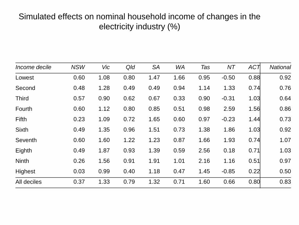
Simulated effects on nominal household income of changes in the
electricity industry (%)
Income decile NSW Vic Qld SA WA Tas NT ACT National
Lowest 0.60 1.08 0.80 1.47 1.66 0.95 -0.50 0.88 0.92
Second 0.48 1.28 0.49 0.49 0.94 1.14 1.33 0.74 0.76
Third 0.57 0.90 0.62 0.67 0.33 0.90 -0.31 1.03 0.64
Fourth 0.60 1.12 0.80 0.85 0.51 0.98 2.59 1.56 0.86
Fifth 0.23 1.09 0.72 1.65 0.60 0.97 -0.23 1.44 0.73
Sixth 0.49 1.35 0.96 1.51 0.73 1.38 1.86 1.03 0.92
Seventh 0.60 1.60 1.22 1.23 0.87 1.66 1.93 0.74 1.07
Eighth 0.49 1.87 0.93 1.39 0.59 2.56 0.18 0.71 1.03
Ninth 0.26 1.56 0.91 1.91 1.01 2.16 1.16 0.51 0.97
Highest 0.03 0.99 0.40 1.18 0.47 1.45 -0.85 0.22 0.50
All deciles 0.37 1.33 0.79 1.32 0.71 1.60 0.66 0.80 0.83
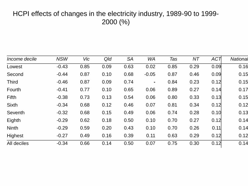
HCPI effects of changes in the electricity industry, 1989-90 to 1999-
2000 (%)
Income decile NSW Vic Qld SA WA Tas NT ACT National
Lowest -0.43 0.85 0.09 0.63 0.02 0.85 0.29 0.09 0.16
Second -0.44 0.87 0.10 0.68 -0.05 0.87 0.46 0.09 0.15
Third -0.46 0.87 0.09 0.74 - 0.84 0.23 0.12 0.15
Fourth -0.41 0.77 0.10 0.65 0.06 0.89 0.27 0.14 0.17
Fifth -0.38 0.73 0.13 0.54 0.06 0.80 0.33 0.13 0.15
Sixth -0.34 0.68 0.12 0.46 0.07 0.81 0.34 0.12 0.12
Seventh -0.32 0.68 0.15 0.49 0.06 0.74 0.28 0.10 0.13
Eighth -0.29 0.62 0.18 0.50 0.10 0.70 0.27 0.12 0.14
Ninth -0.29 0.59 0.20 0.43 0.10 0.70 0.26 0.11 0.14
Highest -0.27 0.49 0.16 0.39 0.11 0.63 0.29 0.12 0.12
All deciles -0.34 0.66 0.14 0.50 0.07 0.75 0.30 0.12 0.14

Real household income effects due to changes in the electricity
industry, 1989-90 to 1999-2000 (%)
Income decile NSW Vic Qld SA WA Tas NT ACT National
Lowest 1.03 0.23 0.71 0.84 1.64 0.09 -0.79 0.79 0.76
Second 0.92 0.40 0.39 -0.19 1.00 0.27 0.87 0.65 0.61
Third 1.04 0.03 0.53 -0.06 0.33 0.05 -0.54 0.91 0.49
Fourth 1.01 0.35 0.70 0.20 0.45 0.09 2.31 1.42 0.69
Fifth 0.61 0.36 0.59 1.10 0.55 0.17 -0.56 1.31 0.58
Sixth 0.83 0.67 0.84 1.04 0.66 0.57 1.51 0.91 0.80
Seventh 0.92 0.91 1.06 0.73 0.82 0.91 1.64 0.64 0.93
Eighth 0.78 1.24 0.74 0.89 0.48 1.84 -0.09 0.59 0.89
Ninth 0.55 0.97 0.70 1.47 0.91 1.45 0.89 0.39 0.82
Highest 0.30 0.50 0.25 0.78 0.36 0.82 -1.13 0.10 0.38
All deciles 0.71 0.66 0.64 0.82 0.65 0.84 0.35 0.69 0.69
Gini coefficient -0.15 0.11 -0.05 0.18 -0.05 0.26 -0.25 -0.22 -0.02

Strengths and limitations of this
approach
– Strengths
• Structurally simple
• Straight forward interpretation
• Flexible
– Limitations
• No feedback effects in the micro-simulation model

An alternative approach
– Incorporate micro-sim model with CGE model
• Internally consistent
• Feedback effects
– Require more work on CGE model and database