ECONOMY-ENERGY- CLIMATE INTERACTION –THE MODEL · PDF fileECONOMY-ENERGY- CLIMATE INTERACTION –THE MODEL WIAGEM- ... Non Technical Abstract ... model WIAGEM, including all world

ECONOMY-ENERGY- CLIMATE INTERACTION –THE MODEL WIAGEM- Claudia Kemfert May 2001 ∗∗ Claudia Kemfert is head of section ”S.P.E.E.D” (Scientific Pool of Environmental Economic

Disciplines) at the Dept. of Economic I , University of Oldenburg.

Address for correspondence:

Dept. of Economic I, Oldenburg University

D- 26111 Oldenburg

E- mail: [email protected]

Tel: +49 441 798 4106

Fax: +49 441 798 4101

Kemfert: The Model WIAGEM 2

Abstract

This paper presents an integrated economy-energy-climate model WIAGEM (World

Integrated Assessment General Equilibrium Model) which incorporates economic, energetic

and climatic modules in an integrated assessment approach. In order to evaluate market and

non –market costs and benefits of climate change WIAGEM combines an economic approach

with a special focus on the international energy market and integrates climate interrelations by

temperature changes and sea level variations. WIAGEM bases on 25 world regions which are

aggregated to 11 trading regions and 14 sectors within each region. The representation of the

economic relations is based on an intertemporal general equilibrium approach and contains

the international markets for oil, coal and gas. The model incorporates all greenhouse gases

(GHG) which influence the potential global temperature, the sea level variation and the

assessed probable impacts in terms of costs and benefits of climate change. Market and non

market damages are evaluated due to the damage costs approaches of Tol (2001).

Additionally, this model includes net changes in GHG emissions from sources and removals

by sinks resulting from land use change and forest activities. This paper describes the model

structure in detail and outlines some general results, especially the impacts of climate change.

As a result, climate change impacts do matter within the next 50 years, developing regions

face high economic losses in terms of welfare and GDP losses. The inclusion of sinks and

other GHG changes results significantly.

Non Technical Abstract

Nearly all scientific reports including the youngest IPCC report confirm once more that the

impact of humankind on the natural environment has never been greater (IPCC 2001) and

cause substantial long term and irreversible climatic changes. One important source of climate

change are the anthropogenic greenhouse gases emissions. Increasing atmospheric

concentrations of greenhouse gases have a substantial impact on the global temperature and

sea level which generate extensive economic, ecological and climatic impacts. These impacts

are investigated by a world integrated assessment modelling tool which combines a detailed

description of the main economic relations with a very simplified model to represent the

climate interlinkages. Model results confirm the investigations by natural scientists: climate

change do matter within the next 50 years and induce substantial impacts to all world regions.


Introduction

Nearly all scientific reports including the youngest IPCC report confirm once more that the

impact of humankind on the natural environment has never been greater (IPCC 2001) and

cause substantial long term and irreversible climatic changes. One important source of climate

change are the anthropogenic greenhouse gases emissions. Increasing atmospheric

concentrations of greenhouse gases have a substantial impact on the global temperature and

sea level which generate extensive economic, ecological and climatic impacts. Potential

impacts of climate change encompass a general reduction in crop yields in most tropical and

sub tropical regions, decreased water availability in water- scarce regions, an expansion in the

number of people exposed to vector and water borne diseases and heat stress, intensification

in the risk of flooding from heavy precipitation events and sea level rise, augmented energy

demand for space cooling due to higher summer temperature; beneficial impacts cover an

increased potential crop yield in some regions at higher latitude, potential rise in global timber

supply from appropriately managed forests, increased water availability, reduced winter

mortality and reduced energy demand for space heating due to higher winter temperatures

(IPCC 2001). Additionally, working group I of the IPCC reports that the global average

surface temperature has risen by 0.6 ± 0.2 °C over the 20th century stressing the fact that the

increase in temperature in the Northern Hemisphere have been the largest of any century

during the past 1,000 years, 1990 was the warmest decade and 1998 the warmest year.

Furthermore, the atmospheric concentration of the greenhouse gases carbon dioxide CO2,

methane CH4 and nitrous oxide N2O increased drastically since 1750.

A comprehensive analysis of all previously described effects caused by climate change need

to be based on a broad and integrated evaluation tool which combines economic, energy and

climate relations in one modelling instrument and so allows an integrated assessment of costs

and benefits of emissions reduction policies. Models based on only economic, ecologic or

climate considerations allow a comprehensive assessment of only one aspect of climate

change. Current models that try to integrate climate interrelations in an economic framework

typically use stylised and reduced interrelations of all domains.

This paper presents a novel integrated assessment modelling approach which is based on a

detailed account of economic relations. The core is an intertemporal general equilibrium

model WIAGEM, including all world regions and the main economic sectors. The general

equilibrium models also includes by a representation of the international energy markets for

oil, coal and gas. The economic model is coupled to a model of the ocean carbon cycle and

climate.


WIAGEM has 25 world regions which are aggregated to 11 trading regions and 14 sectors

within each region. The model incorporates the greenhouse gases (GHG) CO2, CH4 and

N2O, which affect the global temperature, the sea level. In turn, temperature and sea level

determine the impacts of climate change. Market and non market damages are evaluated due

to the damage costs approaches of Tol (2001). Additionally, this model includes net changes

in GHG emissions from sources and removals by sinks resulting from land use change and

forest activities.

The first part of this paper gives a brief overview of existing economic, climatic and

ecosystem-models and integrated assessment approaches. The main focus of this paper is the

description of the integrated assessment model WIAGEM. Primarily, the economic, energy

and the climatic module of the model are explained thoroughly. The paper concludes by a

short illustration of selected key model results.

Integrated Assessment models

The economic assessment of climate change is based on either pure economic models

focusing on economic relations and interlinkages or economic models enlarged by stylised

climatic interrelations or submodels which are usually known as integrated assessment (IAM)

models. Ecological effects like impacts of climate change on biodiversity are mainly modelled

by ecosystem models concentrating on ecological interrealtions (see Prentice et al., 1992,

Haxeltine et al., 1996, Kaplan 2001, Esser et al. 1994, Kaduk 1996 Knorr, 2000, Knorr und

Heimann, 2001); climatic impacts can be assessed chiefly by sophisticated climate models

(Maier-Reimer & Hasselmann 1987, Maier-Reimer 1993, Sarmiento & al 1992, Siegenthaler

1978, Hasselmann & al. 1997, Joos & al 1999, Hooss 2001). Pure economic models base

primarily on a general equilibrium approach based on aggregated world regions which mostly

do not include sectoral disaggregation. Economic model that include sectoral disaggregation

of world regions by a general equilibrium model do mainly not embrace ecological or climatic

interrelations. Economic effects by emissions reduction policies are investigated by Bernstein

und Montgomery (1999), McKibbin and Wilcoxen (1999), Böhringer and Rutherford (1998)

and Kemfert (2000).

Costs and benefits of climate change are predominantly assessed by integrated assessment

models (IAM) incorporating physical relations of climate change and economic effects by

damage functions. Examples for IAMs are MERGE (Manne and Richels 1998), RICE or


DICE (Nordhaus and Yang 1998), CETA (Peck und Teisberg 1991) or FUND (Tol 1998). In

contrast, these models do not include sectoral disaggregation of each world region.

Edmonds (1998) gives an overview of newest modelling approaches, previous overviews can

be found in Dowlatabadi (1993), Dowlatabadi, and Rotmans (1998) and Toth (1995).

Integrated assessment models are characterised by combining multidisciplinary approaches in

order to evaluate impacts by climate change thoroughly. The model presemted in this paper

WIAGEM tries to integrate in a first step a detailed economic model including all world

regions and sectoral disaggregation with an energy and climate submodel. The model includes

all greenhouse gases and potential net emissions changes due to sink potential from land use

change and forestry. The climatic model bases on general interrelations between energy and

non energy related emissions, temperature changes and sea level variations which all induce

substantial economic impacts in terms of market and non market damage costs.


The Model WIAGEM

WIAGEM is an integrated assessment model which combines an economy model based on a

dynamic intertemporal general equilibrium approach combined with an energy market model

and a climatic submodel covering a time horizon of 50 years solving for five years time

steps.1 The basic idea behind this modelling approach is the evaluation of market and non

market impacts induced by climate change. The economy is represented by 25 world regions

which are aggregated to 11 trading regions, each region covers 14 sectors. The sectoral

disaggregation contains five energy sectors: coal, natural gas, crude oil, petroleum and coal

products and electricity. The dynamic international competitive energy market for oil, coal

and gas is modelled by global and regional supply and demand, the oil market is characterised

by imperfect competition with the intention that the OPEC regions can use their market power

to influence market prices. Energy related greenhouse emissions occur as a result of economic

and energy consumption and production activities. At the present time, a number of gases

have been identified as having a positive effect on radiative forcing (IPCC 1996) which are

included in the Kyoto protocol as “basket” of greenhouse gases. The model includes three of

these gases: carbon dioxide (CO2), methane (CH4) and nitrous dioxide (N2O) which are

evaluated to be the most influential greenhouse gases within the short term modelling period

of 50 years. The exclusion of the other gases is not believed to have substantial impacts on the

insights of the analysis.

Because of the short term application of the climate submodel, we consider only the first

atmospheric lifetime of the greenhouse gases, assuming that the remaining emissions have an

infinite life time. The atmospheric concentrations induced by energy related and non energy

related emissions of CO2, CH4 and N2O have impacts on radiative forcing which influence

the potential and actual surface temperature and sea level. Market and non market damages

determine the regional and overall welfare development.

1 The model is written in the computer language GAMS (MPSGE) and solved by the algorithm MILES, see Rutherford (1993)


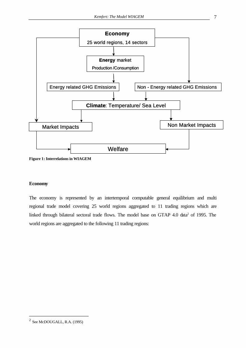
Figure 1: Interrelations in WIAGEM

Economy

The economy is represented by an intertemporal computable general equilibrium and multi

regional trade model covering 25 world regions aggregated to 11 trading regions which are

linked through bilateral sectoral trade flows. The model base on GTAP 4.0 data2 of 1995. The

world regions are aggregated to the following 11 trading regions:

2 See McDOUGALL, R.A. (1995)

Economy

25 world regions, 14 sectors

Energy market

Production /Consumption

Energy related GHG Emissions Non - Energy related GHG Emissions

Market Impacts Non Market Impacts

Climate: Temperature/ Sea Level

Welfare

Economy

25 world regions, 14 sectors

Energy market

Production /Consumption

Energy related GHG Emissions Non - Energy related GHG Emissions

Market Impacts Non Market Impacts

Climate: Temperature/ Sea Level

Welfare


Regions ASIA India and other Asia (Republic of Korea, Indonesia, Malaysia, Philippines,

Singapore, Thailand, China, Hong Kong, Taiwan) CHN China CNA Canada, New Zealand and Australia EU15 European Union JPN Japan LSA Latin America (Mexico, Argentina, Brazil, Chile, Rest of Latin America) MIDE Middle East and North Africa REC Russia , Eastern and Central European Countries ROW Other countries SSA Sub Saharan Africa USA United States of America Table 1: World regions

The economic structure of each region consists of five energy sectors: (1) coal, (2) natural

gas, (3) crude oil, (4) petroleum and coal products and (5) electricity and industrial sectors,

agriculture and services. Because of the intertemporal optimisation framework we explicitly

include a savings good sector. The aggregated factors for production include land, labour and

capital.

All products are demanded by intermediate production, exports, investment and a

representative consumer, market actors behave within a full competition context.

Consumption and investment decisions are based on rational point expectations of future

prices. The representative agent for each region maximises lifetime utility from consumption

which implicitly determines the level of savings. Firms choose investment in order to

maximise the present value of their companies.


Sectors COL Coal CRU Crude Oil GAS Natural Gas EGW Electricity OIL Petroleum and coal products ORE Iron and Steel CRP Chemical Rubber and Plastics NFM Non Ferrous Metals NMM Non Metal mineral Products AGR Agriculture PPP Pulp and Paper TRN Transport industries Y Other manufactures and Services CSG Savings good

Table 2: Sectoral classification

In each region production of the non-energy macro good is captured by an aggregate

production function which characterises technology through transformation possibilities on

the output side and substitution possibilities on the input side between alternative

combinations of inputs. Goods are produced for the domestic and for the export market.

Production of the energy aggregate is described by a CES function which reflects substitution

possibilities for different fossil fuels (i.e., coal, gas, and oil) and capital, labour representing

trade off effects with a constant elasticity of substitution. Fossil fuels are produced from fuel-

specific resources and the non-energy macro good subject to a CES technology.

The CES production structure follows the concept of ETA-MACRO combining nested capital

and labour at lower level. Energy is treated as a substitute of a capital labour composite

determining together with material inputs the overall output (see Figure 2).


Figure 2: Production Structure of sector j in region r

The representative producer of sector j ascertains the CES profit function

[ ] DXDXDX FXDX

jjDXj

Yj papap σσσ −−− −+=Π 1

111 )1(()(

[ ]KLEM

KLKE

KLEM

KL

KLE

KLKLKLEKEM Lj

Kj

RKKj

Ej

Ej

Ej

Mj

Mj

Mj papaapaapa

σσ

σ

σσ

σσσσ

−−

−

−−

−−−−

−+−+−+−1

1

1

1

11

1111 ))(1()()1()1( (1.1)

with:

:DMja Domestic production share of total production by sector j

:Kja Value share of capital within capital –energy composite

Lja : Value share of labour within capital -energy -labour aggregate

:Mja Value share of material within capital-energy-labour material aggregate

pj : Price of domestic good j

pFX: Price of foreign exchange (exchange rate)

pRK: Price of capital

:Ejp Price of energy

Export Good Pxj Domestic good Pd j

OUTPUT Pyj

CET1 τ

Leontief

Other intermediate Inputs Pa1....Pan

Energy- Capital- Labor-Land Composite Input

Energy Pe j Value-added composite

CoalOil/Gas

backstop

Oil Gas

CES σEKLN

Capital Labour Land

CES σ KLNCES σE

CES 2*σE

Export Good Pxj Domestic good Pd j

OUTPUT Pyj

CET1 τ

Leontief

Other intermediate Inputs Pa1....Pan

Energy- Capital- Labor-Land Composite Input

Energy Pe j Value-added composite

CoalOil/Gas

backstop

Oil Gas

CES σEKLN

Capital Labour Land

CES σ KLNCES σE

CES 2*σE


:Mjp Price of material/land

pL: Price of labour

σKE: Substitution elasticity between capital and energy

σKEL: Substitution elasticity between labour and capital and energy composite

σKLEM: Substitution elasticity between material and labour/ capital and energy- composite

Y: Activity level of production sector j.

CET: Constant elasticity of transformation τ

CES: Constant elasticity of substitution σ

A representative agent for each region maximises its region’s discounted utility over the

model’s time horizon (50 years) under budget constraint equating the present value of

consumption demand to the present value of wage income, the value of initial capital stock,

the present value of rents on fossil energy production and tax revenue. In each period

households face the choice between current consumption and future consumption, which can

be purchased via savings. The trade-off between current consumption and savings is given by

a constant intertemporal elasticity of substitution. Producers invest as long as the marginal

return on investment equals the marginal cost of capital formation. The rates of return are

determined by an uniform and endogenous world interest rate such that the marginal

productivity of a unit of investment and a unit of consumption is equalised within and across

countries. The primary factors, capital, labor, and energy are combined to produce output in

period t. In addition, some energy is delivered directly to final consumption. Output is

separated in consumption and investment, investment enhances the (depreciated) capital stock

of the next period. Capital, labor, and the energy resource earn incomes, which are either

spent on consumption or saved. Saving equals investment through the usual identity (see

Figure 3). Protection costs lower other investment in the economy (crowding out).


Figure 3: Dynamic structure

Capital is used for production with a capital price Ktp and an utility price of RK

tp and is

depreciated by rate δ:

1( ) (1 )K K RK K rt t t t tp p p p ptcδ +Π = − + − − (1.2)

with:

Ktp : Price of capital in period t

RKtp : Price of capital services in period t

Kt: Activity level of capital in period t

rtptc : regional protection costs

Investments are produced by Leontief technology:

∑−=Π ++j

Atj

Ij

Kt

It papPp ,11 )( (1.3)

Ija Value share investment of good j

It: Activity level of investments in period t

P: Time period

Labour is supplied by household and demanded by firms, all household are confronted with a

specific time quota be spend for labour or leisure. This labour – leisure decision is determined

by net wages ensuring a price elastic labour supply. One representative agent by each region

demands a composite consumption good produced by combining the Armington good and the

household energy aggregate good according to a CES configuration. σend describes the

elasticity of substitution between the composite macro good and the energy aggregate.

Aggregate end-use energy is composed of oil, gas, and coal with an interfuel elasticity of

substitution equal to one. The backstop fuel is a perfect substitute for the energy aggregate.

Capital, Labour, Energy Output

Period 1

Period 2

Income Savings

Consumption

Investment / Protection costs

Capital

Capital, Labour, Energy Output

Period 1

Period 2

Income Savings

Consumption

Investment / Protection costs

Capital


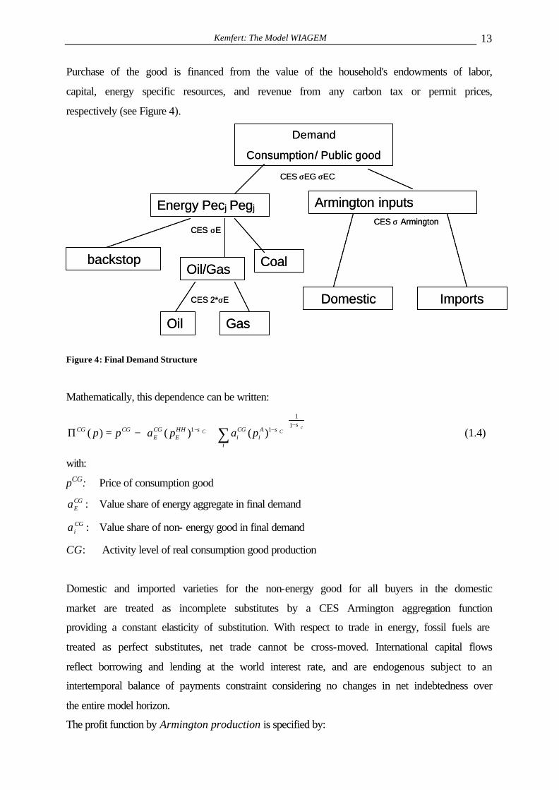
Purchase of the good is financed from the value of the household's endowments of labor,

capital, energy specific resources, and revenue from any carbon tax or permit prices,

respectively (see Figure 4).

Figure 4: Final Demand Structure

Mathematically, this dependence can be written:

cCC

i

Ai

CGi

HHE

CGE

CGCG papappσ

σσ−

−−

+−=Π ∑

11

11 )()()( (1.4)

with:

pCG: Price of consumption good CGEa : Value share of energy aggregate in final demand

CGia : Value share of non- energy good in final demand

CG: Activity level of real consumption good production

Domestic and imported varieties for the non-energy good for all buyers in the domestic

market are treated as incomplete substitutes by a CES Armington aggregation function

providing a constant elasticity of substitution. With respect to trade in energy, fossil fuels are

treated as perfect substitutes, net trade cannot be cross-moved. International capital flows

reflect borrowing and lending at the world interest rate, and are endogenous subject to an

intertemporal balance of payments constraint considering no changes in net indebtedness over

the entire model horizon.

The profit function by Armington production is specified by:

Demand

Consumption/ Public good

Energy Pecj Pegj Armington inputs

CoalOil/Gas

backstop

Oil Gas

CES σ ArmingtonCES σE

CES 2*σE

CES σEG σEC

Domestic Imports

Demand

Consumption/ Public good

Energy Pecj Pegj Armington inputs

CoalOil/Gas

backstop

Oil Gas

CES σ ArmingtonCES σE

CES 2*σE

CES σEG σEC

Domestic Imports


( )[ ] DMDMDM FXA

jjAj

Aj

Aj papapp σσσ −−− −+−=Π 1

111 )1()( (1.5)

with:

:Ajp Price of Armington good j

Aja : Domestically produced good j value share of domestic and import good aggregate

pFX: Price of foreign exchange (exchange rate)

σDM: Substitution elasticity between domestically and imported good

Aj: Armington activity level

Energy

WIAGEM includes four energy production sectors, one non-energy sector and three fossil

fuel sectors traded internationally for oil, gas and coal. Coal production in the OECD and gas

production in Russia grow with energy demand at constant prices. The elasticity of

substitution between the resource input and non-energy inputs is calibrated to meet a given

price elasticity of supply. Exhaustion leads to rising fossil fuel prices at constant demand

quantities. The carbon-free backstop technology establishes an upper bound on the world oil

price, this backstop fuel is a perfect substitute for the three fossil fuels and is available in

infinite supply at one price, which is calculated to be a multiple of the world oil price in the

benchmark year. Demand elasticities depend on back stop technologies, by low backstop

costs demand elasticities are high and vice versa.

A composite energy good is produced by either conventional fossil fuels - oil, gas, and coal –

represented by a nested CES technology (with an elasticity of interfuel substitution σfuel ) or

from a backstop source with Leontief technology structures. Oil and gas can be substituted by

an elasticity of substitution twice as large as the elasticity between their aggregate and coal.

The energy good production is determined by final demand of industry and households .

[ ][ ]

] ] ] ELEFOSSIL

ELE

COA

FOSSILCOA

COAFOSSIL

FOSSILELE

COCOSCOj

SCOj

SCOj

COCOHCOj

HCOj

HCOj

COAj

COCOGASj

GASj

GASj

COCOOILj

OILj

OILj

ELEj

ELEj

ELEj

Ej

Ej

pefpa

pefpaapefpa

pefpaapapp

σσσ

σσ

σ

σσ

σσ

−−−

−−

−

−−

−−

++

++++

+−+−=Π

11

11

11

122,

122,122,

122,1

)(

)()(

)()1()(

(2.1)

With:


ELEja Electricity value share of energy aggregate by sector j

OILja Oil value share of fossil energy aggregate by sector j

GASja Gas value share of fossil energy aggregate by sector j

HCOja Hard coal value share of coal aggregate by sector j

SCOja Soft coal value share of coal aggregate by sector j

σELE Substitution elasticity between electricity and fossil energy

σFOSSIL Substitution elasticity between fossil energy inputs

σCOA: Substitution elasticity between hard and soft coal 2,COOIL

jef CO2 share of oil in sector j

2,COGASjef CO2 share of gas in sector j

2,COHCOjef CO2 share of hard coalin sector j

2,COSCOjef : CO2 share of soft coal in sector j

pCO2 Price of carbon

Ej Activity level of energy production

Demanded energy by households is produced by a CES function:

EGEG

EGi

COCOi

Ai

COHHi

EHH

EHH papapp

σσ

−

=

−

+−=Π ∑

11

1222, )()( (2.2)

with: E

HHia , Value share of energy good i of household

EHHp : Price of energy by household demand

σEG: Substitution elasticities between energy goods

EHH: Activity level of energy production by household

The intertemporal optimal dynamic allocation is characterised by the steady state growth path

which means that in order to reach the equilibrium conditions all sizes have to rise by a same

growth rate. In the long run, conventional energy as fossil fuels are typified by exhaustion

which increases resource prices. We assume that within the future time periods an carbon free

backstop technology will be developed and utilised in order to substitute conventional energy.


Because of that a carbon free backstop technology can be utilised within future times at price

fBS $/t CO2. Zero profit condition is determined by:

BSCGCOBS fpp −=Π 2 (2.3)

with:

pCG: Price of consumption good

fBS: Costs of carbon free energy supply

BS: Activity level of backstop technology

Emission limits can be reached by domestic action or by trading emission permits within

Annex B countries allocated initially due to regional commitment targets. Those countries

meeting the Kyoto emissions reduction target stabilise their mitigated emissions at 2010

level.3

According to regional abatement costs countries will sell or buy emission permits. Countries

facing high abatement costs above permit prices will purchase emission permits, regions with

marginal abatement costs lower than the permit price will vend emission licenses. Revenues

from selling permits are refunded lump-sum back to the representative consumer in the

abating country. Within this context it has to be stressed that problems around the concrete

implementation of the flexible mechanisms and emissions trading scheme, like on

compliance, early crediting and deception in order to influence permit prices are neglected

within the modelling context.

Climate

The model comprises three of the most important anthropogenic greenhouse gases: carbon

dioxide (CO2) which covers over 80 percent of total radiative forcing by anthropogenic

greenhouse gases, methane (CH4) and nitrous oxide (N2O). Primarily due to human activities,

the concentration of these gases in the earth atmosphere have been increasing since the

industrial revolution.

In WIAGEM, we consider the relationship between man made emissions and atmospheric

concentrations and the resulting impact on temperature and sea level. Because of the short

term analysis of considering 50 years up to 2050, we neglect classes of atmospheric

greenhouse gas stocks with different atmospheric lifetimes as modelled usually by the

impulse response function and reduced forms of carbon cycle model developed by Maier-

Reimer and Hasselmann (1987) and applied by Hooss (2001). Energy and non energy related 3 This can be called as “Kyoto forever” scenario


atmospheric concentrations of CO2, CH4 and N2O have an impact on radiative forcing

relative to their base year levels. Energy related emissions are calculated due to the energy

development of each period, energy related CO2 emissions are considered by the emissions

coefficients of the EMF group:

Coal Oil Gas

CO2 Coefficients

in billion metric tons/ Exaj.

0.2412

0.1374

0.1994

Table 3: CO2 Coefficients

Energy related CH4 emissions are determined by the CH4 emissions coefficients of gas and

coal production in billion tons of CH4 per exajoule gas and coal production, the coefficients

are taken from the MERGE model 4.0 (Manne 1998).

Table 4: Emissions coefficients in billion tons of CH4 per exajoule gas production;

Source: MERGE4.0

Table 5: Emissions coefficients in billion tons of CH4 per exajoule coal production

Source: MERGE 4.0.

Non energy related emissions cover parts of the CH4 emissions and N2O emissions. The

global carbon dioxide emissions baseline pathway is assumed to start from 6 to 11 billion tons

of carbon in 2030 which is roughly consistent with the carbon emissions projections of the

IPCC reference case of medium economic growth (IPCC 1996).

Table 6: Non energy related emissions in million tons-1990; Source: MERGE 4.0 , IPCC (1994) and IEA (1998)

USA EU15 JPN CNA FSU CHN MIDE ASIA ROW2000 0,187 0,493 0,000 0,225 1,005 1,170 1,377 0,468 0,9822010 0,168 0,413 0,000 0,222 0,823 0,955 1,121 1,121 0,8052020 0,149 0,333 0,000 0,190 0,641 0,740 0,864 0,864 0,6272030 0,131 0,253 0,000 0,158 0,458 0,524 0,607 0,607 0,4492040 0,112 0,173 0,000 0,126 0,276 0,309 0,350 0,350 0,2712050 0,094 0,094 0,000 0,094 0,094 0,094 0,094 0,094 0,094

USA EU15 JPN CNA FSU CHN MIDE ASIA ROW2000 0,354 0,196 0,000 0,371 0,512 0,963 0,000 0,117 0,3562010 0,354 0,196 0,000 0,371 0,512 0,963 0,000 0,117 0,3562020 0,354 0,196 0,000 0,371 0,512 0,963 0,000 0,117 0,3562030 0,354 0,196 0,000 0,371 0,512 0,963 0,000 0,117 0,3562040 0,354 0,196 0,000 0,371 0,512 0,963 0,000 0,117 0,3562050 0,354 0,196 0,000 0,371 0,512 0,963 0,000 0,117 0,356

USA EU15 JPN CNA FSU CHN MIDE ASIA ROWCH4 25,8 15 1 5 7 43,2 0 46 132N2O 1,1 0,8 0,1 0,3 0,3 0,7 0,2 0,5 1,7


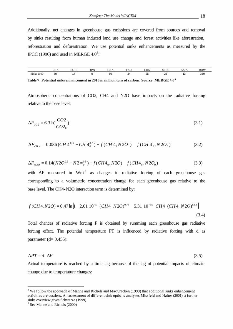
Additionally, net changes in greenhouse gas emissions are covered from sources and removal

by sinks resulting from human induced land use change and forest activities like aforestration,

reforestration and deforestration. We use potential sinks enhancements as measured by the

IPCC (1996) and used in MERGE 4.04:

Table 7: Potential sinks enhancement in 2010 in million tons of carbon; Source: MERGE 4.05

Atmospheric concentrations of CO2, CH4 and N2O have impacts on the radiative forcing

relative to the base level:

)22

ln(3.60

2 COCO

FCO =∆ (3.1)

)2,4()2,4()44(036.0 005.0

05.0

4 ONCHfONCHfCHCHFCH +−−=∆ (3.2)

)2,4()2,4()22(14.0 0005.0

05.0

2 ONCHfONCHfNONF ON +−=−=∆ (3.3)

with ∆F measured in Wm-2 as changes in radiative forcing of each greenhouse gas

corresponding to a volumetric concentration change for each greenhouse gas relative to the

base level. The CH4-N2O interaction term is determined by:

[ ]52.11575.05 )24(41031.5)24(1001.21ln47.0)2,4( ONCHCHONCHONCHf ⋅⋅⋅⋅+⋅⋅⋅+= −−

(3.4)

Total chances of radiative forcing F is obtained by summing each greenhouse gas radiative

forcing effect. The potential temperature PT is influenced by radiative forcing with d as

parameter (d= 0.455):

FdPT ∆⋅=∆ (3.5)

Actual temperature is reached by a time lag because of the lag of potential impacts of climate

change due to tempertature changes:

4 We follow the approach of Manne and Richels and MacCracken (1999) that additional sinks enhencement activities are costless. An assessment of different sink options analyses Missfeld and Haites (2001), a further sinks overview gives Schwarze (1999) 5 See Manne and Richels (2000)

USA EU15 JPN CNA FSU CHN MIDE ASIA ROWSinks 2010 50 17 0 50 34 25 25 13 250


)(1 ttt ATPTtlagATAT ∆−∆⋅=∆−∆ − (3.6)

with tlag as the time lag, ∆Att measures the actual change in temperature in year t relative to

the base year.

Because of the short term analysis of approximately 50 years from now,sea level changes will

change insignificantly during this time period. However, newest calculation estimate a rough

linear relationship between temperature changes and sea leven variations. By assuming that

sea level will vary by 7 cm of 1 °C temperatur change (s=7), we calculate small sea level

changes due to the actual temperature changes: sea level variations are determined by the very

rough estimates of a linear relationship between actual temperature:6

ATsSL ∆⋅=∆ (3.7)

Impacts of climate change cover market and non market damages, the former comprise all

sectoral damages, production impacts, loss of welfare etc, the latter contain ecological effects

like bioviversity losses, migration, natural disasters etc. In order to assess impacts by climate

change we follow the approach of Tol (2001) to cover impacts on forestry, agriculture, water

resources and ecosystem changes as an approximation of a linear relationship between

temperature changes, per capita income or GDP and protection costs due to sea level rise. Tol

(2001) estimates vulnerability of climate change, covering a comprehensive evaluation of

diverse climate change impacts. Besides sctoral impacts on agriculture, forestry, water

resources and energy consumption he covers impacts on ecosystems and mortality due to

vector borne diseases, and cardiovascular and respiratory disorders. We use the assessed

protection costs and use an approximation of potential impacts. Impacts are additional costs to

the economy lowering other investments (crowding out effect). Protection costs due to sea

level rise shows Table 8.

Table 8: Protection costs of one metre sea level rise in 109 $; Source: Tol (2001)

Aggregated impacts of climate change are evaluated by:

0

( )r

r r rtt t t tr

yDAM PT PC

yβα∆ = ⋅ ∆ ⋅ + (3.8)

6 These estimates base on assumptions by the climate model NICCS, Hooss (2001)

USA EU15 JPN CNA FSU CHN ASIA MIDE71,38 136 63 10,79 53 171 305 5


with DAM as total impacts (damages), α and β are parameters, PC represents the sectoral

protection costs due to sea level rise.

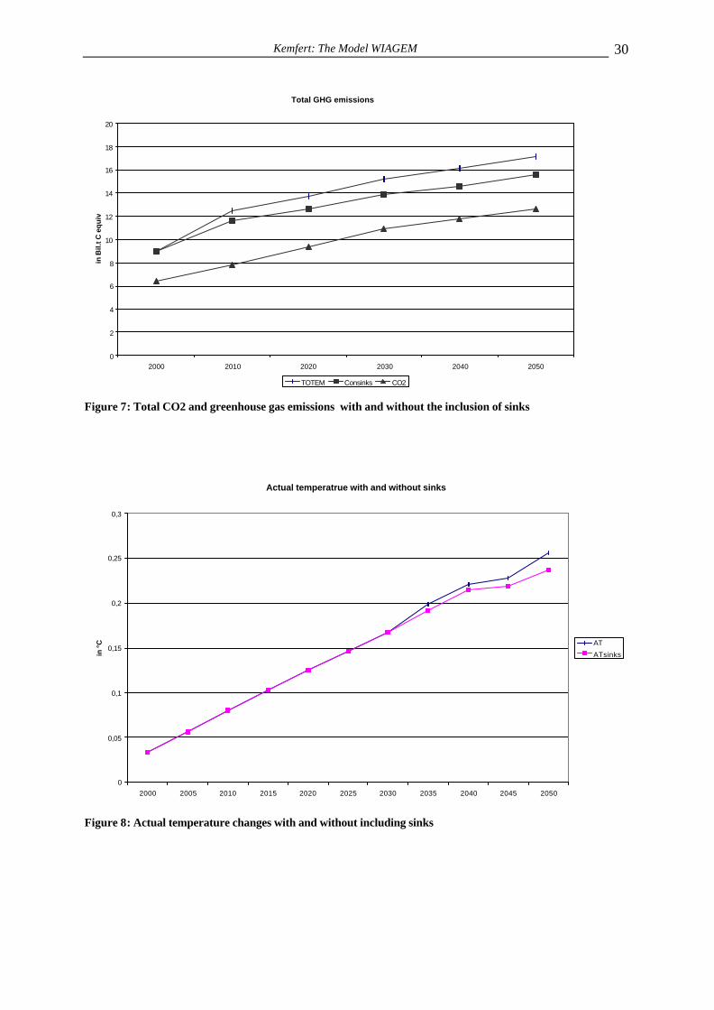
Basic model results Climate Change impacts Climate change impacts do matter within the next 50 years, model results demonstrate that

primarily developing countries have to accept high welfare losses and GDP reductions in

comparison to a scenario where no climate change impacts are included. The CC scenario

describes the Climate Change (CC) scenario and is compared against a scenario where no

climate impacts are evaluated.

Table 9: Welfare in HEV, GDP in % and impacts in % of the CC scenario in comparison to no impact assessment

Developing regions suffer if climate impacts are included because of their vulnerability and

also because of higher percentage impacts of economic values. Relatively poor countries have

to spend higher percentage of their income on protection costs, as a consequence production

losses because of less economic investments are much higher in this regions. Rich countries

like USA or Europe suffer by economic losses in terms of welfare as real income losses and in

terms of GDP reductions, but percentage decreases are not as significant as in developing

regions. As these results demonstrate, climate change impacts do matter even within the next

50 years, primarily developing regions are affected negatively.

Welfare GDP Impacts in%JPN -0,08 -0,02 0,12CHN -1,14 -0,57 3,44USA -0,28 -0,05 0,30SSA -0,82 -0,24 1,45ROW -1,29 -0,31 1,87CNA -0,23 -0,09 0,54EU15 -0,24 -0,06 0,36REC -0,44 -0,08 0,48LSA -0,29 -0,12 0,72ASIA -0,3 -0,18 1,09MIDE -0,04 -0,1 0,60


Kyoto emissions reduction

This section describes some basic model results. The model horizon encompasses 50 years,

the model solves in 5 years time period. By including all greenhouse gases as described in

section 2 of this paper, total GHG emissions increase from roughly 9 billion ton to 17 billion

ton carbon equivalent emissions in 2050 (IPCC emissions scenarios (1999)), see Figure 7.

Regional greenhouse gas emissions differ substantially, the inclusion of the other greenhouse

gases CH4 and N2O raises reference emissions for the European Union from 1.517 in 2010 to

1.894 billion tons of carbon. For the US, the inclusion of sinks lowers the greenhouse gas

emissions from 2.133 to 2.030 in 2010 and 2.686 to 2.496 billion tons of carbon in 2050.

Japan has no significant net emissions changes due to the inclusion of sinks. The global CO2

emissions baseline pathway is assumed to start from 6 to 12,7 billion tons of carbon in 2050

which is roughly consistent with the carbon emissions projections of the IPCC reference case

of medium economic growth (Figure 5 and Figure 6).

The inclusion of sinks lowers total net GHG emissions to roughly 15.5 bil t. carbon equivalent

in 2050 (see Figure 7). Because of the time deceleration of response impacts by potential and

actual temperature changes range from 0.15 to 0.25 °C from 2030 to 2050, the inclusion of

sinks cause comparatively marginal declines of actual temperature after 2030.

Because of the assumed linearity between temperature changes and sea level rise, the

potential sea level increase by 1 cm in 2025 to roughly 1.8 cm in 2050. As seen before, the

incorporation of sinks by land use change and forestry tends to lower this increase marginally

after 2030. These changes are low in comparison to other projected studies (IPCC 2001) and

can be explained mainly by the short term time horizon considered and because of the time

deceleration of response impacts (Figure 9).

Potential impacts by climate change are measured in percentage of global GDP which cover

impacts on forestry, agriculture, water resources and ecosystem changes as an approximation

of a linear relationship between temperature changes, per capita income or GDP and

protection costs due to sea level rise. Emission reduction augments climate change impacts

through warming and sea level rise. Figure 10 compares the impacts of climate change

through the emissions reductions induced by the Kyoto protocol. The emissions reductions

attempt prescribed by the Kyoto protocol causes hugh economic effort by drastic GHG


emissions reductions which induce lower economic impacts of climate change as percentage

of GDP. In terms of impacts in percentage of GDP this means that with the inclusion of sinks

global impacts increase because of less economic welfare losses. Because of hugh economic

efforts that have to be undertaken in order to reach the emissions targets of the Kyoto

protocol, regional welfare declines especially for those regions which have high emissions

reduction targets (Table 10). By the inclusion of sinks as reduced net emissions impacts in

terms of percentage GDP changes increase because of less GHG emissions reduction needs

and therefore less income and GDP losses.

Developing regions suffer by the implementation of the Kyoto protocol and emissions

reduction targets mainly because of international trade spill over effects. Although we allow

international emissions permits trading, economic welfare in terms of the Hicksian equivalent

which explains the real income variation decreases in developed and developing regions. This

is because trading losses as a result of drastic economic efforts by developed regions cause

negative spill over effects. A drastic emissions reduction lowers the demand for energy which

induce a energy price diminution. Regions with high energy import shares could benefit by

this development but countries that face a high share of energy exports will suffer as for

example the coal exporting region China.

Kyoto ALL GHG Kyoto CO2 Kyoto GHG trade Kyoto CO2 trade sinks JPN -0,09 -0,15 -0,05 -0,08 -0,01 CHN -0,08 -0,14 -0,04 -0,09 -0,06 USA -0,35 -0,42 -0,12 -0,19 -0,10 SSA -0,02 -0,01 -0,03 -0,01 -0,05 ROW -0,14 -0,18 -0,05 -0,08 -0,01 CNA -0,08 -0,10 -0,05 -0,07 -0,02 EU15 -0,28 -0,39 -0,18 -0,24 -0,12 REC -0,08 -0,12 0,24 0,33 0,11 LSA -0,02 -0,01 -0,01 -0,01 -0,03 ASIA -0,12 -0,18 -0,09 -0,11 -0,08 MIDE -0,13 -0,19 -0,08 -0,10 -0,01

Table 10: Welfare effects measured in Hicksian equivalent in comparison to the base case

If no emissions permit trading is allowed, as one main seller of emissions permits Russia will

suffer due to high economic losses. Developed regions like EU15 or Japan face high

abatement costs which leads to higher economic losses by meeting the Kyoto emissions

reduction target. If all GHG are included, the number of low costs abatement options are

increased improving the economic situation for OECD regions. Without the allowance of

permit trade, regional welfare impacts are much higher if only CO2 emissions are included.


The negative welfare effect for Russia and Eastern Europe can be explained as follows: the

Russian economy is weak and substantial production and trade efforts are necessary in order

to regain their economic potential. If the Kyoto protocol is implemented, substantial welfare

losses occur to Annex I regions resulting in terms of trade deterioration. In comparison to the

BAU case where no emissions reduction measures are active, Russia`s positive export trends

of for example selling more gas than before cannot overcompensate negative trade spill over

effects coming from economic declines of other strong Annex I countries.

A comparison of a trade versus no trade scenario demonstrates that all countries can benefit

by Annex B permit trading, mainly countries in transition as REC because of the “hot air”

effect. Emissions permit trading better off all Annex B countries as well as non Annex B or

developing countries because of international trade spill over effects. Annex B countries

facing high emissions reduction targets and high domestic marginal abatement like Japan and

USA costs will certainly benefit by Annex B emissions permit trading. Essentially, USA and

EU 15 will trade permits within a full trade scenario because of their high share on total

carbon emissions. The option of permit trade lowers negative welfare impacts, the inclusion

of all GHG bring about a decreasing international permit price which also leads to more

benefits for OECD regions by making imports more attractive relative to domestic emissions

abatement.

The inclusion of sinks and the parallel GHG emissions reduction target forced by the Kyoto

protocol improves the welfare effects in comparison to the Kyoto emissions reduction

scenario without the inclusion of sinks. Especially the oil exporting region OPEC and the

USA and also Canada are benefiting by the inclusion of sinks because of less severe

emissions reductions targets. It improves also the economic welfare impacts in comparison to

the cases where trade is allowed.

Conclusion

The model WIAGEM is an integrated assessment model that build on a detailed economic

intertemporal general equilibrium model covering 25 world regions and 14 sectors of each

world region. It contains an energy submodel that represents the international market for oil,

coal and gas allowing a more realistic representation of the oil market in that sense that the

OPEC regions can influence the oil market price due to their market power. An integrated

assessment of economic, ecological and climate impacts is reached by an incorporation of


climate interlinkages that try to evaluate economic market and non market damages of climate

change. The coverage of all GHG improves the economic welfare impacts especially for

OECD regions as not only the additional options of emissions abatement increase by the

inclusion of all greenhouse gases but also diminishes the international permit price. The

additional inclusion of sinks improves the welfare impacts in comparison to all other

scenarios which leads to higher economic impacts and damages. The conclusion from this

analysis is that on the one hand pure economic effects demonstrate positive impacts of the

inclusion of sinks but on the other hand positive income effects lead also to higher non market

impacts according to the temperature and seal level variations.

Acknowledgement

The Ministry of Science and Culture in Germany gave financial support to this study. All

errors and opinions expressed are solely due to the limitations of the author. I thank Richard

Tol and Alan Manne for very fruitful comments


Literature

Bengtsson, L. & V.Semenov (2000): Secular trends in characteristics of daily precipitation simulated by GCM, in prep.

Berkhout, F., Eames, M. and Skea, J. (1999) Environmental Futures. UK Office of Science and Technology/Foresight Programme.

Bernstein, P., Montgomery, W.D. (1999): Global Impatcs of the Kyoto Agreement: Results from the MS-MRT Model, Paris

Böhringer, C., Rutherford, T.(1999): World Economic Impacts of the Kyoto Protocol, in: Welfens, P., Hillebrand, R. und Ulph, A: Internalization of the Economy, Environmental Problems and New Policy Options

Bruckner, T., G.Petschel-Held, F. L.Toth, H.-M.Fussel, C.Helm, M.Leimbach, and H.-J.Schellnhuber (1999): Climate change decision support and the tolerable windows approach, Environmental Modeling and Assessment 4, p.217-234

Carraro, C. and D. Siniscalco (1998), "International Environmental Agreements: Incentives and Political Economy", European Economic Review

Caspersen, J.P., et al., Contributions of Land-Use History to Carbon Accumulation in U.S. Forests. Science, 2000. 290: p. 1148-1151.

Cramer W., et al. Global response of terrestrial ecosystem structure and function to CO2 and climate change: results from six dynamic global vegetation models. Global Change Biologogy, in press.

Cubasch, U., K.Hasselmann, H.Höck, E.Maier-Reimer, U.Mikolajewicz, B.D.Santer, and R.Sausen (1992): Time-dependent greenhouse warming computations with a coupled ocean-atmosphere model, Climate Dynamics 8, p.55-69

Deke,O., G.Hooss, C.Kasten, G.Klepper, and K.Springer (2000): What's the economic impact of climate change? Simulation results from a coupled climate-economy model, Kiel Working Paper, The Kiel Institute for World economics, in prep.

Dowlatabadi, H., and M. Granger Morgan (1993) "Integrated Assessment of Climate Change." Science 259 (26 March): 1813, 1932.

Edmonds, J (1998): Climate Change Economic Modelling: Background Analysis for the Kyoto Protocol, OECD workshop Paris

Esser, G., Hoffstadt, J., Mack, F. and Wittenberg, U. 1994. High-Resolution Biosphere Model - Documentation. Mitteilungen aus dem Institut für Pflanzenökologie der Justus-Liebig-Universität Gießen, Gießen, Germany.

Haxeltine, A., I.C. Prentice, and D.I. Creswell, A coupled carbon and water flux model to predict vegetation structure. Journal of Vegetation Science, 1996. 7(5): p. 651-666.

IEA (1998): Abatement of Methane Emissions, IEA greenhouse Gas R&D program

IPCC (1992): Climate Change 1992, The Supplementary Report to The IPCC Scientific Assessment (Working Group II) Cambridge University Press, p. 198

IPCC (1996): Climate Change 1995, The Science of Climate Change. Contribution of Working Group I to the Second Assessment Report of the IPCC, Cambridge University Press, p.572

IPCC (1999) Special Report on Emission Scenarios, [http://sres.ciesin.org].


Joos, F., C.Prentice, S.Sitch, R.Meyer, G.Hooss, G.-K.Plattner, and K.Hasselmann (2000): Global warming feedbacks on terrestrial carbon uptake under the IPCC emission scenarios, in preparation

Joos, F.,C.Prentice, S.Sitch, R.Meyer, G.Hooss, G.-K.Plattner, and K.Hasselmann (2000): Global warming feedbacks on terrestrial carbon uptake under the IPCC emission scenarios, in preparation

K.Hasselmann, S.Hasselmann, R.Giering, V.Ocaña, and H.v.Storch (1997): Sensitivity study of optimal CO$_2$ emission paths using a simplified structural integrated assessment model (SIAM), Climatic Change 37, p.345-386

Kaduk, J. 1996. Simulation der Kohlenstoffdynamik der globalen Landbiosphäre mit SILVAN - Modellbeschreibung und Ergebnisse. Max-Planck-Institut für Meteorologie, Examensarbeit Nr. 42, 157 pp.

Kaplan, J. Geophysical Applications of Vegetation Modelling, Dissertation, Universität Lund, Abteilung Pflanzenphysiologie, Lund, Schweden, ISBN 91-7874-089-4, 2001.

Kemfert, C. (1998): Estimated substitution elasticities of a nested CES production function for Germany, Energy Economics, 20, S. 249 – 264

Kemfert, C. (2000): Economic Implications of the Kyoto Protocol ,Perspectives of newest climate change policy options, Environmental Economics (18/2000)

Kemfert, C., Lise, W., Tol, R. Games of Climate Change with International Trade , Research Unit Sustainability and Global Change SGC-7, Centre for Marine and Climate Research, Hamburg University, Hamburg, 2001

Kemfert, C., Tol, R. Equity, international Trade and Climate Policy, Research Unit Sustainability and Global Change SGC-5, Centre for Marine and Climate Research, Hamburg University, Hamburg, 2001

Knorr, W. and M. Heimann, Uncertainties in global terrestrial biosphere modeling. Part I: A comprehensive sensitivity analysis with a new photosynthesis and energy balance scheme. Global Biogeochemical Cycles, 2001. 15(1): p. 207-225.

Knorr, W., Annual and interannual CO2 exchanges of the terrestrial biosphere: process-based simulations and uncertainties. Global Ecology and Biogeography, 2000. 9: p. 225-252.

Lüdeke, M.K.B., et al., The Frankfurt Biosphere Model: a global process-oriented model of seasonal and long-term CO2 exchange between terrestrial ecosystems and the atmosphere. I. Model description and illustrative results for cold deciduous and boreal forests. Climate Research, 1994. 4: p. 143-166.

MacCracken, C.N., Edmonds, J., Kim, S.H., Dands, R.S. (1999): The Economics of the Kykoto Protocol, The Energy Journal, Special Issue of the Costs of the Kyoto protocol: A Multi- Model Evaluation, pp. 25-71

Maier-Reimer, E. (1993): The Biological Pump in the Greenhouse, Global Planetary Climate Change 8, p.13-15

Maier-Reimer, E. and K.Hasselmann, (1987): Transport and Storage of CO2 in the Ocean - An Inorganic Ocean-Circulation Carbon Cycle Model, Clim.Dynam. 2, p.63-90

Manne, A., Mendelsohn, R., Richels, R. (1995): MERGE- A model for evaluating regional and global effects of GHG reduction policies, Energy Policy, 23, 235-274

Manne, A., Richels, R. (1998): The Kyoto Protocol: A cost-effective Strategy for Meeting


Environmental Objectives?

Manne, A., Richels, R.: A Multi-gas Approach to climate policy- with and without GWPs“, 2000

McGuire, A.D. et al., Carbon balance of the terrestrial biosphere in the twentieth century: Analyses of CO2, climate and land-use effects with four process-based ecosystem models. (preprint), 2000.

McKibbin, W., Wilcoxen, P. (1999): Permit Trading under the Kyoto Protocol and Beyond, Paris

Meyer, R., F.Joos, G.Esser, M.Heimann, G.Hooss, G.Kohlmaier, W.Sauf, R.Voss, and U.Wittenberg (1999): The substitution of high-resolution terrestrial biosphere models and carbon sequestration in response to changing CO2 and climate, Global Biogeochemical Cycles 13, p.785-802

Missfeld, F., Haites, E.: The Potential Contribution of Sinks to Meeting the Kyoto Protocol Commitments, 2001

Myers, N. (1988): Threatend biotas: 'hot spots' in tropical forests, Environmentalist, 8(3), 187-208.

Myers, N. (1990): The biodiversity challenge: expanded hot-spots analysis, Environmentalist, 10(4), 243-256.

Nordhaus, W.D. (1993): Rolling the "DICE": An optimal transition path for controlling greenhouse gases, Resource Energy Econ. 15, p.27-50

Nordhaus, W.D., Yang, Z. (1996): RICE: A regional dynamic general equilibrium model of optimal climate change policy, American Economic Review, 86, 741-765

Nordhaus, W:D. (1991): To slow or not to slow: the economics of the greenhouse effect, Econ.J. 101, p.920-937

Peck, S.C. and C.J.Teisberg (1992): CETA: A model for carbon emissions trajectory assessment, Energy J. 13, 55-77

Peck, S.C., Teisberg, T.J. (1991): CETA: A model for carbon emissions trajectory assessment, Energy Journal, 13, 55-77

Petschel-Held, G., H.--J.Schellnhuber, T.Bruckner, F. L.T\'oth, and K.Hasselmann (1999): The Tolerable Windows Approach: Theoretical and Methodological Foundations, Climatic Change 41, p.303-331

Petschel-Held, G.,H.--J.Schellnhuber, T.Bruckner, F. L.T\'oth, and K.Hasselmann (1999): The Tolerable Windows Approach: Theoretical and Methodological Foundations, Climatic Change 41, p.303-331

Potter, C.S., et al., Terrestrial ecosystem production: a process model based on global satellite and surface data. Global Biogeochemical Cycles, 1993. 7(4): p. 811-841.

Prentice, C., et al., A global biome model based on plant physiology and dominance, soil properties and climate. Journal of Biogeography, 1992. 19: p. 117-134

Rotmans, J., and Dowlatabadi, H. (1998), 'Integrated assessment of climate change: evaluation of models and other methods', in Rayner, S. and Malone, E.(eds.), Human choice and climate change: an international social science assessment, Batelle Press, USA.

Rutherford, T. (1993): MILES: A Mixed Inequality and Non-linear Equation Solver


Sarmiento,L., J.C.Orr, and U.Siegenthaler (1992): A perturbation simulation of CO$_2$ uptake in an ocean general circulation model, J.Geophys.Res. 97 C3, p.3621-3645

Schwarze, R. (1999): Biologische Quellen und Senken im Kyoto Protokoll. Ein Plaedoyer fuer die Verknüpfung von internationalem Tropenwald- und Klimaschutz durch den Mechanismus fuer umweltvertraegliche Entwicklung, Discussion paper

Sellers, P.J., et al., A revised land surface parameterization (SiB2) for atmospheric GCMs. Part 2: The generation of global fields of terrestrial biophysical parameters from satellite data. 1995: p. 1-49.

Siegenthaler, U. & H.Oeschger (1978): Predictiong future atmospheric carbon dioxide levels. Science 199, p.388-395.

Sitch, S. The role of vegetation dynamics in the control of atmospheric CO2 content, Dissertation, Universität Lund, Abteilung Pflanzenphysiologie, Lund, Schweden, 2000.

Tol, R. (1999): Temporal and Spatial Efficiency in Climate Policy: Applications of FUND, Environmental and Resource Economics, forthcoming

Tol, R.(2001): Estimates of the damage costs of climate change, part1 and 2

Toth, F.(1996): Practice and progress in integrated assessment of climate change, in: Energy Policy, Vol. 23, No.4/5, pp. 253-267

Voss, R. and U.Mikolajewicz (2000): Long-term climate changes due to increased CO2 concentration in the coupled atmosphere-ocean general circulation model ECHAM3/LSG, Clim.Dyn. in press

Welsch, H. (1996): Klimaschutz, Energiepolitik und Gesamtwirtschaft: Eine allgemeine Gleichgewichtsanalyse für die Europäische Union, München: Oldenbourg

Welsch, H. (1998): Coal Subsidization and Nuclear Phase-out in a General Equilibrium Model for Germany, Energy Economics 20 (1998), 203-222


Regional GHG Emissions

0,0

0,5

1,0

1,5

2,0

2,5

3,0

3,5

4,0

4,5

5,0

2000 2010 2020 2030 2040 2050

bil

lio

n t

of

ca

rbo

n e

qu

iva

len

t

JPN CHN USA SSA ROW CNA EU15 REC LSA ASIA MIDE

Figure 5: Regional greenhouse (GHG) emissions

Figure 6: Regional GHG emissions including sinks

GHG emissions including sinks

0,0

0,5

1,0

1,5

2,0

2,5

3,0

3,5

4,0

4,5

2000 2010 2020 2030 2040 2050

in B

ill.

T o

f c

arb

on

eq

uiv

ale

nt

JPN CHN USA SSA ROW CNA EU15 REC LSA ASIA MIDE


Total GHG emissions

0

2

4

6

8

10

12

14

16

18

20

2000 2010 2020 2030 2040 2050

in B

il.t

C e

qu

iv.

TOTEM Consinks CO2 Figure 7: Total CO2 and greenhouse gas emissions with and without the inclusion of sinks

Actual temperatrue with and without sinks

0

0,05

0,1

0,15

0,2

0,25

0,3

2000 2005 2010 2015 2020 2025 2030 2035 2040 2045 2050

in °

C

AT

ATsinks

Figure 8: Actual temperature changes with and without including sinks


Seal level with and without sinks

0

0,2

0,4

0,6

0,8

1

1,2

1,4

1,6

1,8

2

2000 2005 2010 2015 2020 2025 2030 2035 2040 2045 2050

in c

m

Slsinks SL Figure 9: Sea level changes without and without the inclusion of sinks, in cm

Impacts in percentage of GDP

0

0,5

1

1,5

2

2,5

2000 2005 2010 2015 2020 2025 2030 2035 2040 2045 2050

per

cen

tag

e o

f G

DP

Basis

Kyoto

with Sinks

Figure 10: Impacts of climate change in percentage of global GDP

Documents

ECONOMY-ENERGY- CLIMATE INTERACTION –THE MODEL · PDF fileECONOMY-ENERGY- CLIMATE INTERACTION –THE MODEL WIAGEM- ... Non Technical Abstract ... model WIAGEM, including all world