Economies of aggregate scale in investment

management

Georgios Magkotsios*

Marshall School of Business, University of Southern California

January 15, 2017

Abstract

This paper provides new evidence on the relationship between size and returns in invest-

ment management. The economies of scale at the industry level dominate the economies of

scale at the fund and investment style levels for all types of funds. The driving force for the

connection between fund returns and aggregate size is the competition among managers. Incip-

ient fund classes with a moderate level of competition experience increasing returns to scale.

As the competition for abnormal returns intensifies over time, the cross-section of managerial

talent becomes more homogenous and the opportunities for yielding alpha within the fund class

are depleted. The gradual decline in the opportunities for alpha eventually reverses the returns

to aggregate scale from increasing to decreasing.

Keywords: investment management; alpha; economies of scale; mutual funds; bond funds;

money market funds; hedge funds; index funds; ETF.

JEL Classification Numbers: G11, G12, G23

*Georgios.Magkotsios.2017@marshall.usc.edu. I am grateful to my supervisors Wayne Ferson, Kevin Murphy,

Kenneth Ahern, and Arthur Korteweg.

I. Introduction

The relation between returns and size in investment management is paramount to the evaluation

of managerial performance. Berk and Green (2004) assume diminishing returns to scale for active

managers to show that performance is not persistent, although managers have the ability to yield

abnormal returns. The empirical evidence on returns to scale at the fund level are mixed1. However,

Pástor et al. (2015) show that the returns of equity mutual funds decrease mostly with the aggregate

size of all competing funds, rather than their own size. I extend their analysis to other classes of

funds, and show that fund returns may increase or decrease with aggregate size. My results are

consistent with a hypothesis of diminishing opportunities for alpha within each fund class.

competition hypothesis? (liquidity and information are both related to competition)

diminishing alpha hypothesis

Pástor et al. (2015) discuss the diminishing returns to aggregate scale in the context of liquidity.

As the equity fund industry grows over time en masse, individual managers have gradually a larger

impact on prices. This effect impedes their ability in outperforming passive strategies, and the

opportunities for yielding alpha within the fund class become more elusive.

Garleanu and Pedersen (2016)model a competition amongmanagers within inefficient markets,

and propose an alternative explanation for the emergence of diseconomies of aggregate scale. As

the equity fund industry grows, the markets become more efficient and the comparative advantage

of informed managers attenuates.

I propose an alternative channel for the effect of aggregate size on fund returns. This channel

relies on the co-evolution of aggregate scale with the cross-sectional distribution in talent among

incumbents. The cross-sectional dispersion in managerial talent is a proxy for the remaining op-

portunities for alpha within the fund class. When managers are alike in talent, it is more strenuous

to outperform their peers and yield superior returns. The hypothesis is that the competition among

1Chen et al. (2004), Yan (2008), Pollet and Wilson (2008), and Pástor et al. (2015) document decreasing returns,

while Elton et al. (2012) show increasing returns with size for equity mutual funds. More later, including no returns to

scale.

1

managers and the dynamics of entry and exit result in a population of incumbents that becomes

progressively more homogeneous. The dispersion in talent should be correlated both with individ-

ual fund returns and aggregate size. As the fund class acquires a larger fraction of market size over

time, the increased competition among managers depletes the opportunities for alpha by decreas-

ing the dispersion of talent. The diminishing returns to aggregate scale emerge from the scarcity

in opportunities for alpha at the industry level. The scarcity in alpha and the growing competition

among managers results in increasing costs of active investing for all incumbents. These costs are

not related to the trading cost from turnover at the fund level. On the contrary, they are independent

of the choice of investment strategy and affect all managers equivalently.

The connection between industry-wide opportunities for alpha, increased costs, and diminishing

fund returns is a little different compared to Pástor et al. (2015). The managers in Pástor et al. face

increasing costs with aggregate scale because their strategies have an incremental impact on market

prices. When the fund class has a small total size altogether, the atomistic managers should have

no effect on prices and there should be no connection with returns and aggregate size. On the

contrary, my hypothesis about the effects of talent dispersion implies that there should always be a

connection between the competition among managers and aggregate scale.

Incipient fund classes have small aggregate size and should be less competitive. A moderate

competition also implies the potential for a large dispersion in cross-sectional talent, at least during

the early stages of the industry’s life cycle. This in turn implies an abundance of opportunities

for alpha within the fund class, since the managers in the upper tail of the distribution have the

potential to outperform their peers at relatively low cost. In addition, the managers at the lower tail

of the distribution are forced to improve by decreasing their costs, since they lack a comparative

advantage in talent. If they are unsuccessful in reducing costs and consistently underperform with

respect to their peers, the investors will force them to exit through capital outflows. As a result,

a moderate competition among managers can improve fund returns for every manager within the

class by decreasing the cost of active investing. This translates to increasing returns to aggregate

scale, a result that is not predicted by the models of Pástor and Stambaugh (2012) or Garleanu and

2

Pedersen (2016).

II. The data

The data involve an ensemble of multiple databases that cover seven distinct fund classes. Each

fund class is distinguished by its unique set of risk factors, reflecting the underlying assets that the

funds invest on. These classes are equity funds, bond funds, money market funds, hedge funds,

index funds, and exchange-traded funds (ETFs).

A. CRSP data

The Survivor-Bias-Free Mutual Fund Database from the Center for Research in Security Prices

(CRSP) is the data source for all fund classes except hedge funds. The time series for each fund

includes its monthly total returns per share mret, net asset value per share mnav, and total net

assets mtna as of month end. The first date is December 1961. However, many funds before

March 1993 have only quarterly values for their total net assets and monthly for their net asset

value. I use linear interpolation with mnav to fill in the regularly-gridded missing values in mtna

from quarterly reporting. I accept interpolated mtna values when the result lies between the two

actual data values at the start and end of the quarter, otherwise I assume constant assets. In addition

to the regularly-gridded missing values from quarterly reporting for early funds in the data, CRSP

has multiple scattered missing values of the total assets. If the time series includes values for mtna

in the previous month and a return mret for the current month, then I fill in the current assets by

assuming no monthly flows from investors. If the return is also missing, then I assume constant

assets. Finally, funds with missing or duplicate dates in their time series are excluded.

The CRSP summary file contains all historic updates on supplementary fund information such

as fund name, style, expense and turnover ratios. The fee structure includes the fund’s monthly

expense ratio and trading costs. The trading cost is given by the round-trip cost per transaction

multiplied with the fund’s turnover ratio. I assume a round-trip cost of 1%. This is the same as

3

in Pástor and Stambaugh (2002), and it is very close to the estimate of 0.95% in Carhart (1997).

CRSP utilizes the 4-letter objective code crsp_obj_cd to unify the Wiesenberger, Strategic Insight,

Lipper, and Thomson Reuters objective and class codes that characterize the fund styles.

The updates on the supplemental information have varying frequency among funds. I merge

the time series and summary files by assuming constant values over time for the supplementary

information in between updates. In addition, CRSP assigns a different fund identifier for each

of the share classes of a single fund (operated by the same fund manager). I use the fund name

to consolidate all the share classes under a single fund, and reassign to the fund a new and unique

identifier. The separators for share classes include the rightmost semicolon (;) or slash (/) characters

in the fund name. Previous studies have used the colon (:) as a share class separator too. However,

the colon character in CRSP is also used to designate fund family names, and its use may result in

incorrect consolidations of different fund managers within the same family of funds. The fund level

returns are calculated as weighted averages of the returns from each share class, where the weights

are the total net assets of each class. The total assets at the fund level is simply the aggregate of all

assets from the share classes.

The 4-letter CRSP objective code crsp_obj_cd by itself is not always adequate to classify a

fund within a fund class, because of data errors and sporadic changes in investment style over time.

Certain keywords in the fund name are used to properly classify funds. I include all CRSP codes

with ED as the first two letters for US equity mutual funds, including cap-based, style-oriented,

and sector funds. The only exception are real estate funds (EDSR), because a subset of them

trade REITs and they tend to be riskier on average than the stock market. I remove funds with the

following keywords in their name: index, ETF, real estate, mortgage bond, fixed, yield, “ muni”2,

money, m/m, cash, liq, and foreign place keywords such as euro, asia, Japan, “Canad”, pacific,

world, foreign, int’l, and international. In addition, I require that the majority of a fund’s assets be

invested in equity, to exclude alternative mutual funds from the equity class.

The fixed income-related keywords above are used to classify funds in the domestic bond fund

2The leading blank allows equity funds that focus on the communications sector, but excludes municipal bond

funds that have erroneously an equity objective code.

4

class, except those that imply short-term debt. These are: money, m/m, cash, liq, and “short term”.

The objective codes for the bond class are: I , IU , IUS, IUI , IUH , IC, ICQH , ICQM , ICQY ,

ICDS, ICDI , IG, IGT , IGD, IGDS, and IGDI . The keywords that are related to short term

debt and the objective codes IM and IMM are used to identify money market funds. Index funds

are identified by the keywords “index”, while ETFs are found with the use of the dummy variable

etf lag and the keywords “etf”, “exchange traded”, and “exchange-traded” respectively. There are

no restrictions on the objective code for index funds and ETFs. I require a minimum expense ratio

of 1 basis point for all funds from CRSP.

B. Hedge fund data

The features of the hedge fund data are significantly different than those of mutual funds.

Hedge funds are subject to fewer regulatory restrictions, and reporting of information to commer-

cial databases is voluntary. Contrary to mutual funds, there is no unique vendor that covers the

majority of the hedge fund universe. For instance, Lipper TASS covers approximately one third of

this universe (Agarwal et al., 2009). The empirical literature has documented multiple biases on

this data. Fung and Hsieh (2000) classify biases that emerge either due to sampling from an unob-

servable population of funds that reflects the underlying structure of the industry and the voluntary

nature of disclosure, or from the process of information collection by the data vendors.

The voluntary disclosure and the different criteria for inclusion among data vendors results in

selection biases. A selection bias implies that the sample in a database does not fully reflect the

features of the true population of hedge funds. It is likely that the best performers voluntarily

report to the vendors to signal their performance to investors and attract new capital, while the

worst performers would choose to conceal their returns. On the other hand, a fraction of the top

performersmay choose to stop reporting once the fund’s goals have been reached and no new capital

is needed. Selection biases may also arise from the vendors’ inclusion criteria. For instance, not

all databases accept managed futures funds. In addition, there exists geographical clustering for

regions other than US and Europe. Most of the funds in Brazil are listed in TASS, while HFR and

5

Morningstar CISDM cover the majority of Chinese funds. HFR also covers the majority of funds

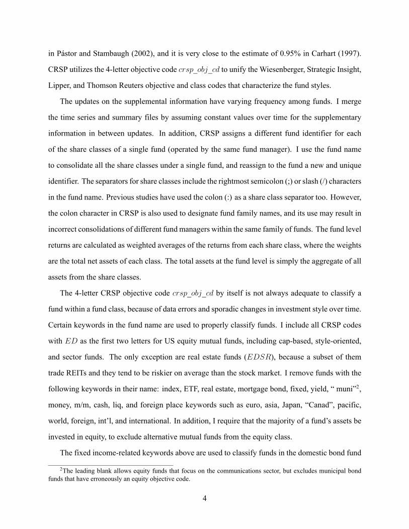
in Japan and South Africa. In order to alleviate the selection bias problem, I merge the hedge fund

data from HFR, TASS, and CISDM that are available through the Wharton Research Data System

(WRDS). The combination of multiple databases improves the convergence of my sample to the

true population of hedge funds, compared to sampling from a single database.

The data licensing inWRDS is different than the direct commercial licenses from these vendors.

Fund name and other supplementary information is either limited or unavailable. To avoid double-

counting of funds that are listed in more than one database, I compare the corresponding time

series of total net assets and returns across all funds from different databases. I accept a match

across databases when the overlapping series for both assets and returns differ by less than 10%.

Figure 1 shows a Venn diagram that illustrates the outcome of the merging process among these

three databases. Once a match is found, I extend the time series to the longest available for the new

fund, including data available for non-overlapping months too.

The hedge fund data from every vendor before 1994 included only active funds at the end of

the sample period, a collection method that resulted in data with survivorship biases. The direction

of the bias is hard to assess, because some funds become defunct after poor performance while

others may cease to report once they don’t need investor capital. The survivorship bias cannot be

fully mitigated, because it is a linked with the underlying structure and evolution of the hedge fund

industry and voluntary reporting (Fung and Hsieh, 2002). I accept fund data after January, 1994,

when the vendors began including defunct funds in their data.

Another bias in hedge fund data is the backfill or “instant history” bias. It involves the back-

dating of the fund’s performance before it started reporting to a vendor. The backfill bias most

often stems from an incubation period for the fund, where seed capital is usually provided by the

manager’s close circle of contacts.3 Fung and Hsieh (2002) find that the average incubation period

in TASS is 12 months. However, there exist cases where the gap between the fund’s inception and

the date that it was first added to the database exceeds 10 years. Previous studies have considered

3Evans (2010) shows that incubation in mutual funds may also result in backfill bias.

6

TASS33.47%

HFR39.30%

CISDM26.02%

0.21%

0.09%

0.27% 0.64%

Figure 1

The total number of unique funds at the 10% level of accuracy among CISDM, HFR, and TASS

is 57659. The percentages in the Venn diagram illustrate the fractions of single-, dual-, and triple-

listed funds across these databases.

7

fund data only after the date that it started to report, to eliminate the backfill bias. However, this

practice may result in a substantial loss of information Fung and Hsieh (2009). In addition, the

WRDS version of CISDM does not list the date that the funds were added to the sample. I apply

the following rule to balance the tradeoff between the backfill bias and the informational loss from

removing observations. I begin with a test date that is 12 months past the first date of the fund’s

time series. If the test date is subsequent to the date that the fund was added to the database, then the

latter becomes the official starting date for my sample. Otherwise, the test date becomes the start-

ing date. This ensures that the discarded observations either comprise the full time period before

the fund was added to the database, or are a maximum of one year after the fund’s inception.

Hedge funds charge a management fee as a percentage of assets under management, and may

also include incentive fees that are contingent on performance. The incentive fees may also include

a high-water mark and a hurdle rate. Incentive fees in my sample are collected after the fund has

completed a full calendar year, with the proceeds spread throughout the next year from January to

December. Missing values for the management fee, incentive fee, and the hurdle rate are replaced

by 2%, 20%, and 0.5% respectively. I also use the currency exchange rates from theH.10Release by

the FED to convert the values of the fund assets from foreign denominations to US dollar amounts.

I consolidate the fund styles in seven broad categories, each involving the following sub-styles

from the various databases:

1. Arbitrage: event driven, relative value, convertible arbitrage, fixed income arbitrage, debt

arbitrage, merger arbitrage, diversified arbitrage, currency, and distressed securities

2. Hedging: equity hedge, dedicated short bias, long/short equity hedge, bear market equity,

biased, and any instance of “hedged” or “long/short” in the style field

3. Multi-strategy: multistrategy, CTA, managed futures, systematic futures, options, volatility

4. Emerging Markets

5. Fund of Funds

8

6. Macro

The hedge fund data vendors also list fund of funds (FOF) in their database. I include the assets

that are managed by funds of funds in the estimation of aggregate size, because this is capital that

investors allocate indirectly to the hedge fund industry. However, I exclude these fund from the

rest of my analysis, because their business model and fee structure are different than that of regular

hedge funds.

C. Factor-mimicking portfolios

I assume a unique set of factor-mimicking portfolios for each fund class. I use the q-factor

model of Hou et al. (2015) for equity funds. The q-factor data extend to 1967. For the period 1962

to 1966 I substitute the four q factors with the four factors from Carhart (1997). The market return

and size factors are common between the two databases. However, the corresponding market return

factors differ by 10% on average.

The empirical factors for asset classes other than equity are not well established in the literature.

Fama and French (1993) showed that a credit risk and a term structure factor explain bond returns

better than their three equity factors. The term structure factor is equivalent to the level factor in

traditional term structure models. However, these two factors cannot explain well the returns of

junk bonds. Elton et al. (1995) showed that the effect of the term structure factor is captured by

an aggregate bond index and the stock market excess return. I use the market return and relative

differences of the Barclays US Aggregate Bond Index for investment-grade bonds, which is an

update to the Lehman index that is used in Elton et al. (1995). The inception date for the Barclays

index is January, 1976. I substitute the index with a term risk factor for dates before that. The

term risk factor is similar to that in Chen et al. (2010), namely the difference between the Treasury

Constant Maturity 10-year and 1-year rates from the H.15 Release by the FED. The default risk

factor is the credit spread between the Baa and Aaa bonds, also available by the H.15 Release.

I also use relative differences of the Barclays US Corporate High Yield Bond Index for junk

bonds. Its inception date is July, 1983. I extend the junk bond factor back to January, 1977 with

9

the High Yield Bond Index return of Blume et al. (1991). They created their high-yield factor

with data from the Drexel Burnham Lambert investment bank. The DBL bank pioneered the junk

bond market starting in 1977. Since junk bonds did not exist before that, I use two separate factor

models for bond funds. The first spans the period 1962-1976 and does not use a high-yield factor.

The second ranges from 1977 to the end of the sample, and uses the consolidated high-yield factor.

Similarly to Elton et al. (1995), I use a macro factor to capture the unexpected changes in

expectations about the US economy that could affect the interest rates. The factor combines the

monthly relative changes in the Conference Board Composite of 4 Coincident Indicators Index

with the lagged relative changes in the survey of Expected Business Conditions for Next Year by

the University of Michigan. The Conference Board (CB) composite index comprises the effects of

coincident indicators on non-agricultural labor, personal income less transfer payments, industrial

production, and manufacturing and trade sales. The factor captures the surprise effect to investors

and consumers, defined as the percent changes in the realized economy minus the lagged percent

changes in the expectations about the economy for the following year. The benefit of using CB

indices is the monthly frequency of data, contrary to real GNP, inflation, or other macro factors that

are available only at a quarterly frequency.

The factor model for the money market funds uses the Federal Funds rate as a proxy to money

market indices, the stock market excess return, and the macro factor defined above. The index fund

and ETF classes are the de facto representatives of passive investment strategies. A regression of

their return on the return of the index that they track should have a zero intercept. For simplicity, I

use the stock market excess return for all index and ETF funds.

In this paper, I consider all hedge funds as a single class, and use a single set of factors to

evaluate their performance. This set is a variation of the seven-factor model of Fung and Hsieh

(2004). I use the stock market excess return and size factors of Hou et al. (2015) for equity strate-

gies, the investment-grade aggregate bond index and default risk factors as defined previously for

fixed income strategies, the commodity and currency trend-following factors from Fung and Hsieh

(2001) for the corresponding strategies, and the macro factor for the unexpected changes in the US

10

economy.

The choice of a single set of factors for hedge funds is not unique in the empirical literature.

Patton and Ramadorai (2013) use the Bayesian Information Criterion to fit the best two out of

four Fung-Hsieh factors for each style. However, the fund style is also voluntarily reported by the

manager to the data vendors, and is not updated over time along with the return and asset time

series for the fund. It is possible that the reported style does not encompass the full set of strategies

that the fund is using. For these cases, the self-reported style may induce the cherry-picking bias

that Sensoy (2009) documents for mutual funds, where the manager attempts to choose a niche

benchmark that can easily outperform. The cherry-picking bias may be coupled with selection

biases for hedge fund alphas. For instance, a manager may start reporting to HFR while he is

already outperforming the HFRI index. The addition of his fund to the database would signal to

investors his superior performance in the HFR universe of funds.

The absence of updates over time for the fund style and other supplementary information with

the vendor may result in stale information. In turn, this could induce a “stale information bias” to

the fund’s alpha if a style-specific set of factors is used, or any other specialization that focuses

on fund features (e.g. leverage). Finally, the common regulatory regime that hedge funds operate

on and the similar fee structure that is independent of style reinforces my choice of a single set of

factors for all hedge funds.

III. Empirical analysis

A. Variable definitions

I define below the variables that I use in my analysis. Summary statistics are shown in Table

1. The data for all fund classes have monthly frequency. The variables at the fund level are Fund

Age (in years), the fund’s assets under management Fund Size (in millions), the net return plus

expense ratio Gross Return, and the net return plus expense ratio minus the benchmark return

Gross Alpha. The latter is a measure of the manager’s talent in active investing, and reflects his

11

potential in outperforming the benchmark return for the corresponding fund class. The fund alpha is

the intercept from expanding window regressions of the fund’s Gross Return on the class-specific

benchmark portfolios. The expanding window regressions for young funds may result in large

measurement errors for the alphas. If an estimate for alpha during a month is more than 100%,

then I reject it and adopt the estimate during the previous month. This is equivalent to the investors

ignoring the latest innovation about the manager’s talent.

Similarly to Pástor et al. (2015), I inflate the monthly values of Fund Size to December 2015 US

dollars using the ratio of the stock market capitalization on December 2015 over the capitalization

at the time of the observation. This inflator aims to capture the size of the fund relative to the

universe of assets that the fund could buy at time t − 1. Funds in every class are included in the

sample only after they exceed for the first time a threshold of $10million in December 2015 dollars.

The Fund Size is allowed to fall below this threshold subsequently, but all observations before the

first time that the fund exceeds the threshold are ignored.

The aggregate variables for each fund class include the total number of funds Total Funds and

the Industry Ratio. This ratio is defined as the sum of the assets under management across all funds

within the class, divided by the total market capitalization. The Industry Ratio captures the effect

of the total size for the class relative to the size of the market where the funds operate. For equity

funds, hedge funds, index funds, and ETFs it is the US stock market. For bond funds and money

market funds it is the US debt market.

The cross-sectional dispersion of Gross Alpha during a month is Std(Gross Alpha). This is the

main variable for this paper. It shows the dispersion of managerial talent within the fund class.

More importantly, it is a proxy for the remaining opportunities in generating alpha within the class.

A large dispersion implies that certain incumbents are distinctly superior than their peers, and have

the potential to yield large risk-adjusted returns. It also implies the potential for large negative

alphas from managers at the left tail of the distribution. On the contrary, a small dispersion in

talent within the class implies that all managers are alike in talent, and it is difficult for anyone

to outperform his peers. I assume that a manager’s talent is exogenous and does not change over

12

time. As a result, the cross-sectional dispersion of talent may only change from the entry and exit

of funds.

B. Diminishing returns to scale within fund classes

Table 2 shows the relation between fund returns and size, measured at the fund and industry

levels. The table presents two estimations for each specification. The first involves OLS regres-

sions with fund fixed effects, and the second implements regressions with recursively demeaned

(RD) variables. The fixed effects capture the unobserved variables for each fund, such as man-

agerial talent. The talent should be correlated both with size and with returns. All variables in

the RD estimations are forward- demeaned to alleviate the finite sample bias. I instrument the

forward-demeaned Fund Size using its backward-demeaned value as an instrument4.

The first two regressions in Table 2 show the relation between Gross Alpha and lagged values

of Fund Size. The coefficient on Fund Size expresses the economies of scale at the fund level.

Most of the estimates appear to be statistically significant. However, the coefficient values are

economically very small. For instance, the RD estimates in regression (2) imply that an increase

of $100 million in the assets under management for a bond fund would result in a decrease of 1 bp

per year in the fund’s return. A similar increase for an equity fund would enhance its performance

by 1.7 bp per year.

The coefficient on Fund Size in the RD estimation for equity funds is positive and significant,

implying increasing returns to scale. This result seems inconsistent with the main assumption of

diminishing returns to scale in Berk andGreen (2004). Previous empirical evidence on the existence

of diseconomies of scale in equity mutual funds are mixed. For instance, some of the studies

documenting decreasing returns to fund size include Chen et al. (2004), Yan (2008), and Pollet and

Wilson (2008). On the other hand, Elton et al. (2012) document increasing returns to fund size.

Regressions (3) and (4) in Table 2 show the relation between a fund’s return and the lagged value

of Industry Ratio. The correlation between a fund’s return and Industry Ratio reflects economies

4The reader is referred to Hjalmarsson (2010) and Pástor et al. (2015) for a detailed discussion and simulation

exercises regarding the RD regressions.

13

of scale at the aggregate level. Regressions (5) and (6) include Fund Size and Industry Ratio. The

first panel in Table 2 verifies the empirical results of Pástor et al. (2015) for equity funds. A typical

value of Industry Ratio for equity funds during the period 2010-2015 is approximately 0.2, which

implies that equity funds manage nearly 20% of the total capital that is available in the US stock

market. The estimates on Industry Ratio imply a 2.7 bp loss in monthly risk-adjusted gross returns

(0.33% per year) on average for every fund, if the equity mutual fund industry were to increase

by 10% with respect to the stock market. These figures are much more economically important

than the returns to scale at the fund level. This indicates that the economies of scale in investment

management operate at the aggregate level, rather than at the fund level.

The liquidity hypothesis states that the profitable investment opportunities within a fund class

are in finite supply. The scarcity in opportunities stems from the regulatory restrictions that are

imposed on the funds and limit the set of permissible active strategies. The diminishing returns at

the industry level emerge from the depletion of these opportunities. As the fund class grows and the

competition among managers intensifies, more funds will chase the same investment opportunities.

Although eachmanager is atomistic and cannot impact prices on his own, the profitable investments

become costlier and more elusive as an increasing number of managers push prices in the same

direction.

The opportunities to outperform in the information hypothesis of Garleanu and Pedersen are

depleted as a larger amount of capital is allocated to informed managers and markets become more

efficient. The aggregate size within the fund class grows when the cost of active investing de-

creases. The cost of active investing includes both the search cost for the investors and the man-

agerial cost of obtaining information about profitable opportunities. The investors gradually make

markets more efficient and attenuate the comparative advantage of informed managers by allocat-

ing to them more capital. This mechanism also implies diminishing returns to aggregate scale for

all incumbent managers. In summary, both the liquidity and the information hypotheses can explain

the diseconomies of aggregate scale for equity mutual funds.

The second and third panels in Table 2 show the effect of size on returns for index mutual funds

14

and exchange-traded funds. These funds represent passive strategies and are not expected to seek

abnormal returns. The dependent variable is Gross Return, defined as the fund’s return with the

expense ratio added back. The coefficients on Fund Size and Industry Ratio in regressions (1) to

(6) are statistically insignificant, suggesting that there exist no economies of scale. The result is

consistent with the liquidity hypothesis. Passive strategies neither require managerial talent nor

they deplete any opportunities for alpha. Therefore, any increases in size should have no effect

on the fund returns. This result is also compatible with the information hypothesis. The passive

managers have no effect on the market’s informational efficiency, and any increase in their capital

should not affect the fund returns across the fund class.

C. Increasing returns to scale within fund classes

Table 2 also shows the relationship between fund performance and aggregate size for hedge

funds, bond mutual funds, and money market funds. The correlation between Industry Ratio and

Gross Alpha is positive for these fund types. This striking result indicates that these funds experi-

ence increasing returns to scale at the aggregate level. In particular, the growth of these industries

coincides with an increase in the expected returns for all incumbent funds. Figure 2 shows the

monthly time series of Industry Ratio for all fund classes. The figure also includes some proxies

for the competition among managers such as the total number of funds, the Average Gross Alpha,

and the cross-sectional dispersion Std(Gross Alpha). The Industry Ratio and Total Funds have an

increasing trend, with equity funds experiencing the steepest growth in market share during the

1990s. The number of funds seems to plateau for every fund class, except for hedge funds where

it seems to decline after the financial crisis of 2007. The fluctuations in the cross section of Gross

Alpha are weakened throughout the life cycle of every fund class. This is also reflected by the

decreasing trend for Std(Gross Alpha).

Increasing returns to aggregate scale in the liquidity hypothesis may arise when small and less

competitive fund classes exploit the opportunities for abnormal returns that would otherwise be

too costly to pursue for investors. For instance, hedge funds have existed for many years before

15

Figure 2

Monthly time series of Industry Ratio (top panel), total number of funds Total Funds (middle panel), and trend component of the cross-

sectional dispersion in gross alpha Std(Gross Alpha) (bottom panel) for equity, bond, money market, and hedge funds. The curve for the

number of hedge funds in the middle panel shows half the corresponding number of funds in the sample for clarity. I extract the trend

component of Std(Gross Alpha) using the Hodrick-Prescott filter with smoothing parameter λ = 129, 600. The shaded areas indicate theNBER recession periods in the United States.

16

the dot-com crisis, but they started to grow substantially following the crash. This growth was

fueled by the transition of the investor base from high-net-worth individuals and family funds to

large institutional investors that were transferring capital from equity funds5. The argument of

the liquidity hypothesis is that hedge funds provided fresh liquidity on investing strategies that

were in demand during that time, but previously unavailable to institutional investors on a wide

scale (e.g. shorting). It is plausible that the liquidity that was originated by institutional capital

increased the returns for all hedge funds by decreasing their cost of active trading. Jame (2016)

shows supporting evidence of larger returns for liquidity-supplying hedge funds. The hedge fund

industry in my sample peaks in size and number of funds before the financial crisis of 2008, and

has been shrinking following the event (Figure 2). The maximum Industry Ratio that the fund class

achieved with respect to the US stock market is 0.156, which is lower than that of domestic equity

funds. This number could be smaller if the sample is restricted to hedge funds with a domicile

within the US. The increasing returns to aggregate scale for hedge funds imply that the industry

has not depleted its opportunities for alpha.

The increasing returns to scale are puzzling for the information hypothesis. The results suggest

that either the market becomes less efficient as the hedge fund industry grows and the informed

managers oversee a larger fraction of the total size, or that more efficient markets can result in larger

returns for the average fund. An increasing fraction of capital among informed managers cannot

plausibly make the markets less efficient. The second case is also implausible. The acquisition

of information is the comparative advantage of active managers against passive indexing. More

efficient markets weaken this advantage, and should thus decrease the excess returns from active

investing. If increased returns were to coexist with more efficient markets, then there must be an

additional underlying mechanism that compensates for the loss of informational value. As a result,

the information hypothesis by itself cannot explain the increasing returns to aggregate scale. Cao

et al. (2016) show that the holdings of levered hedge funds that were brokered by Lehman Brothers

experienced declines in price efficiency during the financial crisis. However, they also show that

5See Fung and Hsieh (2012) for a review of the hedge fund industry.

17

hedge fund ownership of stocks results in improved efficiency on average.

Talent in active investing and alpha for bond funds and money market funds is defined just as in

any other fund class. Interest rate risk exists even for short-term debt, and for long-term debt credit

risk is also a factor. In addition, bond funds and money market funds tend to hold derivatives in

their portfolios (Schulte et al., 2016). As a result, some funds may be able to provide larger yields

to investors than others.

The intuition about the increasing returns to scale in bond and money market funds is similar

to that for hedge funds. Their popularity increased during the 1980s. The investor demand for

fixed income funds during this decade arguably emerged from the rampant inflation and fierce bear

market in equities that had followed the oil price shocks during the 1970s. The liquidity hypothesis

justifies the growth of fixed income funds as an alternative channel to institutional capital. These

fund classes created a market and provided liquidity that allowed the institutional investors to avoid

the side effects of prolonged inflation. However, both fund classes were later surpassed in total

capital by the equity funds, because of the stock market rally during the 1990s (Figure 2).

According to the liquidity hypothesis, the increasing returns to aggregate scale for bond and

money market funds indicate that there exist remaining profitable opportunities through active in-

vesting. In other words, the aggregate size for each of the fund classes is not “large” enough yet to

deplete the opportunities for alpha. During the period 1980-2015, the sum of the Industry Ratio for

bond and money market funds ranged from 10% to 17% with respect to the total US debt market.

In contrast, the equity funds have been managing nearly 20% of the total US stock market capi-

talization. However, this percentage could be larger if it was possible to isolate the aggregate size

of stocks that are traded in exchanges from that of shares that are held by executives and are not

traded. These differences can potentially justify why fixed income funds operate under increasing

returns, while equity funds experience diseconomies of aggregate scale.

18

D. The effect of competition

The liquidity hypothesis suggests that the competition among managers is the foundation for

the economies of aggregate scale. The counterfactual conditional is the single manager setup of

Berk and Green (2004), where there are no effects from competition. If this were true, then the

returns to aggregate scale should be explained by a superposition of fund-level economies of scale.

Specifically, the coefficients for Fund Size and Industry Ratio in Table 2 should have similar values.

However, the table shows that these coefficients have quite different values for each fund class.

The critical feature of the liquidity hypothesis is the scarcity in opportunities for alpha. The

hypothesis implies the following evolution for a fund class. The managers provide liquidity to

investors and there exist plenty of opportunities for profitable investments within incipient fund

classes. However, the competition eventually depletes these opportunities as the fund classmatures.

I use the cross-sectional dispersion of fund alphas during a month Std(Gross Alpha) as a proxy for

the remaining opportunities within a fund class. A manager’s alpha measures his exogenous talent

in active investing. Any changes in Std(Gross Alpha) over time stem from fund entries and exits.

Large values of Std(Gross Alpha) imply that the managers in the upper tail of the cross-sectional

distribution can outperform their rivals and generate large abnormal returns. On the contrary, small

values of Std(Gross Alpha) imply a homogeneity in managerial talent. If managers are alike in

talent, then it is harder to outperform their opponents. Therefore, the homogeneity in talent induces

the scarcity in opportunities for alpha.

Throughout the life cycle of a fund class there exists a non-monotonic relation between excess

returns and aggregate size. The liquidity supply and talent dispersion in nascent classes decrease

the trading costs for all managers and boost their returns. As the aggregate capital and the number

of managers increase over time, more opportunities for abnormal returns are exploited. During this

stage of the life cycle, the fund class experiences increasing returns to aggregate scale. However,

the returns to aggregate scale ultimately reverse to decreasing as the fund class grows and Std(Gross

Alpha) diminishes. The following relations among returns, economies of aggregate scale and op-

19

portunities for alpha capture this mechanism.

∂αit+1

∂σt

> 0 (1)

∂2αit+1

∂σt∂Qt

> 0 (2)

where αit+1 is the expected Gross Alpha for fund i at time t + 1, while σt and Qt are Std(Gross

Alpha) and Industry Ratio respectively at time t.

The dispersion of Gross Alpha is related to the heterogeneity of talent among the incumbent

managers. A large heterogeneity connotes an abundance in opportunities for alpha within the class.

As the dispersion of talent decreases, the incumbent managers become more homogenous and trade

in similar ways. This increases progressively the costs of trading, and the opportunities for alpha

becomemore elusive. As a result, equation (1) states that the expected abnormal returns are smaller

for decreasing Std(Gross Alpha).

Themanagers within an early fund class create a newmarket and exploit profitable opportunities

that would be costlier to investors otherwise. Therefore, the returns to aggregate scale ∂αit+1/∂Qt

are positive initially. Equation (2) states that ∂αit+1/∂Qt decreases as the opportunities for alpha

deplete. Since the managers deplete the opportunities for alpha over time, equation (2) implies that

the returns to aggregate scale may reverse from positive to negative as the fund class matures.

Table 3 shows the effects of competition on the returns to aggregate scale for equity, hedge,

bond, and money market funds. The dependent variable in every regression is Gross Alpha. I de-

trend the Industry Ratio using the filter of Hodrick and Prescott (1997)6, because the correlation

between the trend component of Industry Ratio and Total Funds overshadows every other correla-

tion (see also Figure 2). Regressions (1) and (2) show the effect of the cross-sectional dispersion in

managerial talent, as a proxy for the remaining opportunities to yield alpha within the fund class.

The coefficient for Std(Gross Alpha) is positive for equity mutual funds and hedge funds. This

result verifies equation (2) and it is consistent with the liquidity hypothesis.

6I set the smoothing parameter for the filter to λ = 129, 600, as Ravn and Uhlig (2002) recommend for monthlydata.

20

The coefficient for Std(Gross Alpha) is negative and significant for fixed income funds, but it

becomes insignificant in regressions (5) and (6). This seems inconsistent with the liquidity hypoth-

esis, but it does not rule it out. It is plausible that the managers of bond and money market funds are

not the only agents that supply liquidity to investors for fixed income markets. External liquidity

may stem from central banks through quantitative easing programs, governmental interventions, or

managing firms of money market funds with reputational concerns that prevent them from breaking

the buck. This liquidity is exogenous to the managers, and it may bias downward the coefficient

for Std(Gross Alpha). The downward bias appears because the external liquidity is provided during

bad states of the economy to maintain stability. The expected returns are low during such states.

The external liquidity can increase the dispersion in talent by preserving managers at the lower

tail of the talent distribution that should otherwise have exited. This implies a negative bias in the

correlation between expected returns and Std(Gross Alpha).

The effect of the opportunities for alpha on the economies of aggregate scale is captured by the

interaction between Industry Ratio and Std(Gross Alpha). Regressions (1) and (2) show a positive

correlation for all active fund classes. This verifies equation (2) and it is consistent with the liquidity

hypothesis. I omit the interaction of Std(Gross Alpha) with the trend component of Industry Ratio,

because it is not significant. The results indicate that the sensitivity of fund alphas to aggregate

scale diminishes as the remaining opportunities for alpha within the fund class deplete over time.

They also suggest that the sensitivity can reverse from positive to negative. The reversion of the

sign implies that even the most talented managers shall eventually yield lower abnormal returns in

expectation, due to the scarcity in profitable opportunities within the fund class.

Regressions (3) and (4) focus on the effect of the number of incumbent managers, which is a

proxy for the intensity of the competition within the fund class. The direct effect of Total Funds

on the fund alphas is negative for equity funds and positive for the other fund classes. Recall from

Table 2 that equity funds have decreasing returns to aggregate scale, while hedge and fixed income

funds have increasing returns to aggregate scale. The negative sign for equity mutual funds in

regressions (3) and (4) at Table 3 suggests that the addition of new funds intensifies the competition

21

for the limited profitable opportunities, and therefore decreases the expected abnormal returns for

the average fund. On the contrary, the positive sign for the rest of the fund classes in the same

regressions suggests that the addition of new funds enhances the supply of liquidity to investors

and helps decreasing the trading costs for all incumbents. As a result, the expected abnormal returns

increase for the average fund.

The returns to aggregate scale are negatively correlated with Total Funds for equity and money

market funds, and positively for hedge and bond funds. However, Table 3 shows only the interaction

of Total Funds with the cyclical component of Industry Ratio. The corresponding coefficient for

the interaction of Total Funds with the trend component for Industry Ratio is negatively correlated

and statistically significant for every fund class. This interaction dominates in absolute value the

interactions shown in the table. As a result, Total Funds is overall negatively correlated with the

returns to aggregate scale. This implies that the economies of aggregate scale are larger within less

competitive fund classes, which is consistent with the liquidity hypothesis and the depletion of the

opportunities for alpha from competition.

E. The life cycle of equity mutual funds

I demonstrate below how the returns to aggregate scale vary throughout the life cycle of equity

mutual funds. Table 4 shows regressions similar to those in the first panel of Table 2. The first year

in the sample for all regressions is 1985. This choice avoids the bear markets during the 1970s and

focuses on the stock rally during the 1990s and the aftermath of the dot-com and financial crises of

2007 respectively. Each panel involves a different cutoff year, corresponding to a different stage of

the fund class evolution. The returns to fund size in regressions (1) and (2) are economically small,

regardless of the life cycle stage. The coefficients for Industry Ratio are negative in regressions (3)

and (4), but positive in regression (5).

Figure 3 extends the selected estimations of Table 4 to annual frequency. The independent

variable in these plots corresponds to the cutoff year for the estimation sample. The first year

for all samples is 1985. The black and red points correspond to estimates for Industry Ratio with

22

Figure 3

Returns to aggregate scale throughout the life cycle of equity mutual funds. The dependent variable is the coefficient of Industry Ratio

from regressions similar to those in Table 4. The first year in the sample for all regressions is 1985. The x-axis values correspond to the

sample end year. I use black and red colors for estimates with t-statistic above and below 2 respectively. The shaded areas indicate the

NBER recession periods in the United States.

23

t-statistic above and below 2 respectively. The main result is that the returns to aggregate scale

decrease during the stock market rally of the 1990s. This is consistent with equation (2) and the

liquidity hypothesis. The results of regression (6) imply that the returns to scale have reversed

from positive to negative, although the t-statistics are relatively low. Regressions (3) and (4) yield

negative estimates, suggesting that the initial growth for the industry may precede 1985. However,

regression (5) includes additional control variables and shows positive estimates during this period.

The liquidity hypothesis discusses the long term effects on the returns to aggregate scale during

the life cycle of a fund class. Figure 3 shows how recession periods that have business cycle

frequency can perturb the long term trends of the fund class life cycle. Market crashes may involve

investor demand shocks that can impact Industry Ratio through fund outflows. In addition, a market

crash may also cause multiple funds to exit, which would affect the talent distribution among the

remaining incumbents. Regressions (3) and (4) include only Industry Ratio in their specification.

The left panel of Figure 3 shows how the stock market crashes in 2001 and 2007-2008 impact the

economies of aggregate scale. However, regressions (5) and (6) include additional controls such

as the growth in the number of funds, past excess fund returns, and fund age. These specifications

show that the returns to aggregate scale are relatively unaffected by business cycle shocks.

IV. Robustness

A. Investment style effects

The main results suggest that the excess returns of the average fund are more sensitive to in-

dustry size than the fund’s own size. To identify the origin of the economies of scale, it is useful to

examine whether the effects of competition within a particular investment style are economically

more important than the industry effects across the full fund class. My classification of funds into

classes stems from the risk of the traded securities, similarities in the fee structure, and the reg-

ulatory regime that applies to the funds. Based on these features, I use a common set of factors

for all funds within a class to adjust their returns for risk. This classification implies that the dis-

24

tinction among investment styles within a fund class is irrelevant, and all managers share the same

opportunities in generating abnormal returns.

I test below for cases where some investment styles involve niche strategies that isolate the

opportunities for alpha to a subset of managers. For instance, the main results consider hedge

funds as a single fund class. It is plausible though that macro funds are inherently different than

long-short equity funds, and the opportunities for alpha between these styles do not overlap. The

investment styles for each fund class are summarized in Table 5.

Table 6 shows the sensitivity of Gross Alpha on Industry Ratio as before, and also includes the

sensitivity on Style Ratio. The latter is defined similarly to Industry Ratio, but the aggregate size

spans the funds of a specific investment style instead of all the funds within the class. For instance,

all equity funds share a common Industry Ratio, but funds in each of the cap-based, growth, growth

and income, or sector investment styles have their own Style Ratio. The effect of Style Ratio for

equity funds is negative and significant in models (1) and (2). However, when the specification

includes both aggregate ratios the Style Ratio changes sign, while Industry Ratio becomes more

negative. This implies that the diseconomies of scale operate at the industry level for this class of

funds, and the different styles do not affect the distribution of the opportunities for alpha across

managers.

The results for index and exchange traded funds are statistically insignificant across styles.

These fund classes represent passive investing. The style separates the funds that track equity

indices from those that track fixed income indices. As a result, the gross returns of the average

passive fund are not sensitive to economies of scale.

The fourth panel of Table 6 demonstrates the dominance of industry scale over style effects for

hedge funds. The positive and significant coefficients for Style Ratio in models (1) and (2) become

insignificant in models (5) and (6), while the effect of Industry Ratio remains the same (compare

models (4) and (6)). This is an indication that the economies of scale operate at the industry level

for this class, and all funds share the same opportunities for alpha regardless of investment style.

This is a quite surprising result, because the investment style of hedge funds cover a wide range

25

of strategies and underlying assets of varying risk. It also suggests that a common factor model to

benchmark hedge fund returns is more appropriate than style-specialized factor models.

The Industry Ratio dominates Style Ratio for bond funds too. The effect of the former is similar

across models (3) to (6), while Style Ratio changes its sign when compared to the Industry Ratio.

The interpretation of this result is similar to the intuition about hedge funds. On the other hand, the

comparison between Style Ratio and Industry Ratio for money market funds gives mixed results.

The OLS estimation with fund fixed effects in regression (5) implies that Style Ratio dominates

the effect of Industry Ratio. The coefficient for the former is similar to that for model (1), while

the coefficient for Industry Ratio is statistically insignificant. However, regression (6) implies that

the economies of scale operate at the aggregate level, instead of the style level. The coefficient for

Style Ratio is insignificant and the one for Industry Ratio has similar value to those in regressions

(3) and (4).

The liquidity hypothesis states that the economies of aggregate scale operate within a group

of funds with the same investment opportunities. I group the government, municipal, and prime

money market funds in a single class for my main analysis. It is plausible though that prime funds

are inherently different than funds that restrict their assets to government securities only. For in-

stance, Kacperczyk and Schnabl (2013) assume that government money market funds are riskless

and unaffected by business cycle effects. They restrict their analysis to prime money market funds,

and show that these funds experienced a huge growth in their investment opportunities during the

period 2007-2010. However, the implications of the liquidity hypothesis for money market funds

are valid, irrespective of the level where economies of aggregate scale operate (industry or invest-

ment style). The excess returns of the average money market fund increase with aggregate size,

reflecting the availability of profitable investment opportunities.

B. Other robustness tests

I examine below the robustness of the main results on economies of aggregate scale. I do

not tabulate these tests to save space. The choice of Industry Ratio is a proxy for liquidity at the

26

aggregate level, because it compares the aggregate assets under management with the relevant

total market that is accessible to the managers and investors. To test the sensitivity of the results

on historical market conditions, I perform two robustness tests. First, I replace Industry Ratio with

Industry Size, the aggregate size within the fund class in $trillions. This removes the effects of the

market capitalization from sample. In the second test, I restore Industry Ratio and set a common

starting year for all fund classes. This guarantees that all fund types experience the same market

conditions over time. The results on the economies of aggregate scale remain the same. Equity

mutual funds have diminishing returns, while hedge funds and fixed income funds have increasing

returns with aggregate scale. I also use filters other than the Hodrick-Prescott to detrend Industry

Ratio and replace size-related variables with their logarithms, without any changes to the main

results.

I estimateGross Alpha as the intercept from expanding window regressions of the fund’sGross

Return on the benchmark for the fund class. The expanding window method utilizes the full in-

formation set that is revealed over time for each fund, which is similar in principle to Bayesian

updating in learning models. An additional estimation of alphas utilizes rolling regressions with a

24-month window. The disadvantage of rolling window regressions is the loss of data compared to

the expanding window method, especially for funds with small track records. On the other hand,

the expanding window regressions for young funds may result in large measurement errors for the

alphas. The main results are robust to the estimation method for fund alphas.

The choice of benchmark portfolios for each class in the estimation of Gross Alpha could also

affect the results. I replace the q-factor model of Hou et al. (2015) for equity mutual funds with

the four-factor model of Carhart (1997), and the results remain robust. However, Berk and van

Binsbergen (2015) argue that factor portfolios are not an appropriate benchmark, and use instead

a combination of index funds that are managed by the Vanguard Group. Similarly to Berk and

van Binsbergen, I benchmark the classes of equity and hedge funds using the Capital Asset Pricing

Model (Sharpe, 1964; Lintner, 1965). The benefit of adjusting for risk with the CAPM is that it

captures the profitable opportunities that investors would receive at low cost, had they not invested

27

in active funds. The disadvantage is that, unlike the factor models, the CAPM fails in explaining

adequately the cross section of stock returns (Fama and French, 1993; Hou et al., 2015). As a result,

passive benchmarks could induce spuriously large alphas for the active managers. The economies

of aggregate scale for the CAPM-adjusted equity mutual fund and hedge fund excess returns remain

the same as in the main results.

Fung and Hsieh (2000) suggest that the returns from funds of funds (FOFs) are useful as a

benchmark index for hedge funds, since they represent investor preferences more accurately than

ordinary hedge funds. However, FOFs have a different fee structure than other hedge funds, and

they maintain large cash reserves that they don’t invest. The extraction of the operational costs

from portfolio management by FOFs is not straightforward, and the estimation of Gross Alpha for

these funds can be downward biased (Fung and Hsieh, 2000). Using an index of FOF returns in

my sample yields mixed results for the returns to aggregate scale. The coefficient of Industry Ratio

is negative and significant when this variable is the only one in the specification, and it becomes

insignificant when Fund Size and other control variables are used. On the other hand, the lack of

data on the dual fee structure and cash reserves of funds of funds may induce measurement errors

in the estimation of Gross Alpha.

28

References

Agarwal, Vikas, Naveen D. Daniel, and Narayan Y. Naik, 2009, Role of managerial incentives and

discretion in hedge fund performance, Journal of Finance 64, 2221–2256.

Berk, Jonathan B., and Richard C. Green, 2004, Mutual fund flows and performance in rational

markets, Journal of Political Economy 112, 1269–1295.

Berk, Jonathan B., and Jules H. van Binsbergen, 2015, Measuring skill in the mutual fund industry,

Journal of Financial Economics 118, 1–20.

Blume, Marshall E., Donald B. Keim, and Sandeep A. Patel, 1991, Returns and volatility of low-

grade bonds 1977–1989, Journal of Finance 46, 49–74.

Cao, Charles, Bing Liang, Andrew W. Lo, and Lubomir Petrasek, 2016, Hedge fund holdings and

stock market efficiency,Working paper .

Carhart, MarkM., 1997, On persistence inmutual fund performance, Journal of Finance 52, 57–82.

Chen, Joseph, Harrison Hong, Ming Huang, and Jeffrey D. Kubik, 2004, Does fund size erode

mutual fund performance? the role of liquidity and organization, American Economic Review

94, 1276–1302.

Chen, Yong, Wayne Ferson, and Helen Peters, 2010, Measuring the timing ability and performance

of bond mutual funds, Journal of Financial Economics 98, 72–89.

Elton, Edwin J., Martin J. Gruber, and Christopher R. Blake, 1995, Fundamental economic vari-

ables, expected returns, and bond fund performance, Journal of Finance 50, 1229–1256.

Elton, Edwin J., Martin J. Gruber, and Christopher R. Blake, 2012, Does mutual fund size matter?

the relationship between size and performance, Review of Asset Pricing Studies 2, 31–55.

Evans, Richard B., 2010, Mutual fund incubation, Journal of Finance 65, 1581–1611.

Fama, E. F., and K. R. French, 1993, Common risk factors in the returns on stocks and bonds,

Journal of Financial Economics 33, 3–56.

Fung, William, and David A. Hsieh, 2000, Performance characteristics of hedge funds and com-

modity funds: Natural vs. spurious biases, Journal of Financial and Quantitative Analysis 35,

291–307.

Fung, William, and David A. Hsieh, 2001, The risk in hedge fund strategies: theory and evidence

from trend followers, Review of Financial Studies 14, 313–341.

Fung, William, and David A. Hsieh, 2002, Hedge-fund benchmarks: Information content and bi-

ases, Financial Analysts Journal 58, 22–34.

Fung, William, and David A. Hsieh, 2004, Hedge fund benchmarks: A risk-based approach, Fi-

nancial Analysts Journal 60, 65–80.

29

Fung, William, and David A. Hsieh, 2009, Measurement biases in hedge fund performance data:

An update, Financial Analysts Journal 65, 36–38.

Fung, William, and David A. Hsieh, 2012, Hedge funds, in George M. Constantinides, Milton

Harris, and René M. Stulz, eds., Handbook of the Economics of Finance, volume 2B, chapter 16,

1063–1126 (North-Holland).

Garleanu, Nicolae, and Lasse H. Pedersen, 2016, Efficiently inefficient markets for assets and asset

management, Working paper .

Hjalmarsson, Erik, 2010, Predicting global stock returns, Journal of Financial and Quantitative

Analysis 45, 49–80.

Hodrick, Robert J., and Edward C. Prescott, 1997, Postwar u.s. business cycles: An empirical

investigation, Journal of Money, Credit and Banking 29, 1–16.

Hou, Kewei, Chen Xue, and Lu Zhang, 2015, Digesting anomalies: An investment approach, Re-

view of Financial Studies 28, 650–705.

Jame, Russell, 2016, Liquidity provision and the cross-section of hedge fund returns, Working

paper .

Kacperczyk, Marcin, and Philipp Schnabl, 2013, How safe are money market funds?, Quarterly

Journal of Economics 128, 1073–1122.

Lintner, John, 1965, The valuation of risk assets and the selection of risky investments in stock

portfolios and capital budgets, Review of Economics and Statistics 47, 13–37.

Pástor, Ľuboš, and Robert F. Stambaugh, 2002, Investing in equity mutual funds, Journal of Fi-

nancial Economics 63, 351–380.

Pástor, Ľuboš, and Robert F. Stambaugh, 2012, On the size of the active management industry,

Journal of Political Economy 120, 740–781.

Pástor, Ľuboš, Robert F. Stambaugh, and Lucian A. Taylor, 2015, Scale and skill in active manage-

ment, Journal of Financial Economics 116, 23–45.

Patton, Andrew J., and Ta Ramadorai, 2013, On the high-frequency dynamics of hedge fund risk

exposures, Journal of Finance 68, 597–635.

Pollet, Joshua M., and Mungo Wilson, 2008, How does size affect mutual fund behavior?, Journal

of Finance 63, 2941–2969.

Ravn, Morten O., and Harald Uhlig, 2002, On adjusting the hodrick-prescott filter for the frequency

of observations, Review of Economics and Statistics 84, 371–376.

Schulte, Dominik, Markus Natter, Martin Rohleder, and Marco Wilkens, 2016, Bond mutual funds

and complex investments, Working paper .

30

Sensoy, Berk A., 2009, Performance evaluation and self-designated benchmark indexes in the mu-

tual fund industry, Journal of Financial Economics 92, 25–39.

Sharpe, William F., 1964, Capital asset pprices: A theory of market equilibrium under conditions

of risk, Journal of Finance 19, 425–442.

Yan, Xuemin (Sterling), 2008, Liquidity, investment style, and the relation between fund size and

fund performance, Journal of Financial and Quantitative Analysis 43, 741–767.

31

Table 1Summary statistics for all fund classes.

The starting year for equity, bond, and index funds is 1962, for money market funds is 1973, for private equity firms is 1978, for hedge funds is

1994, and for ETFs is 1995. The sample end date is December, 2015. The unit of observation is the fund-month for all classes but private equity,

where data are listed by the fund’s vintage year. All returns and investor flows are in units of fraction per month, excluding private equity where

a single return is given for each fund. Age is the number of years since the fund’s starting date in the sample (defined in Section II). Fund Size is

the fund’s assets under management in millions. Value Added is defined by the product of the lagged size and the realized gross alpha. It represents

the capital that the manager extracted from the markets during a period. Value Growth is the monthly percent growth in the fund’s value added.

Gross Return is the fund’s return before fees. Gross Alpha is the fund’s return before fees in excess of the class benchmark. Flow is the net of all

monthly investor inflows and outflows for the fund. Total Funds is the number of incumbent funds within the class for a given month, and Fund

Growth is the monthly percent growth in Total Funds. Average Size and Std(Fund Size) are the cross-sectional mean and standard deviation of

the incumbents’ Fund Size for each month. Industry Size is the monthly aggregate Fund Size. Industry Ratio is Industry Size divided by the total

market capitalization, where the total market depends on the fund class and it includes the US stock and/or debt markets. Average Gross Alpha and

Std(Gross Alpha) are the cross-sectional mean and standard deviation respectively of the incumbents’ Gross Alpha during a month. The summary

statistics columns from left to right correspond to the number of observations N, the sample mean, standard deviation, minimum, maximum, and

the first-order autocorrelation AR1.

N Mean SD Min Max AR1

Equity Funds

Age (yr) 768,761 10.043 9.523 0.000 53.917 0.244

Log(Fund Size) 762,890 5.794 1.935 −6.005 12.975 0.315

Log(Value Growth) 341,387 −2.521 1.755 −15.911 11.478 0.141

Gross Return 759,199 0.006 0.054 −0.753 1.696 0.726

Gross Alpha 753,670 0.002 0.021 −0.995 0.998 0.033

Flow 751,896 0.010 0.092 −1.023 24.474 0.102

Total Funds (1000s) 649 1.193 1.037 0.125 2.770 1.000

Fund Growth (%) 648 0.481 1.926 −6.250 24.074 −0.040

Average Size ($bn) 649 3.224 2.073 1.445 12.304 0.992

Log(Std(Fund Size)) 649 9.009 0.369 8.388 10.024 0.991

Industry Size ($tn) 649 2.455 1.640 0.651 5.532 0.999

Industry Ratio 649 0.096 0.064 0.025 0.215 0.999

Average Gross Alpha 647 0.001 0.003 −0.037 0.023 0.348

Std(Gross Alpha) 647 0.019 0.021 0.003 0.173 0.393

Bond Funds

Age (yr) 586,589 10.411 8.542 0.000 53.917 0.422

Log(Fund Size) 584,094 5.826 1.743 −5.829 13.002 0.351

Log(Value Growth) 243,037 −2.503 1.797 −14.362 10.759 0.308

Gross Return 584,908 0.003 0.017 −0.899 0.862 0.518

Gross Alpha 581,243 −0.004 0.047 −0.999 0.992 0.101

Flow 580,051 0.009 0.269 −1.005 196.357 0.036

Total Funds (1000s) 649 0.909 0.806 0.021 1.994 1.000

Fund Growth (%) 648 0.712 3.142 −1.961 38.605 −0.017

Average Size ($bn) 649 1.872 0.760 0.534 4.742 0.989

Log(Std(Fund Size)) 649 8.265 0.604 7.268 9.526 0.996

Industry Size ($tn) 649 1.407 1.210 0.041 3.983 0.997

Industry Ratio 649 0.033 0.028 0.001 0.087 0.999

Average Gross Alpha 647 −0.001 0.031 −0.270 0.363 0.699

Std(Gross Alpha) 647 0.048 0.053 0.005 0.516 0.798

32

Table 1 – continued from previous page

N Mean SD Min Max AR1

Money Market Funds

Age (yr) 286,177 10.638 7.969 0.000 41.917 0.578

Log(Fund Size) 277,054 6.968 1.825 −5.155 13.189 0.243

Log(Value Growth) 115,848 −2.529 1.651 −14.473 12.613 0.227

Gross Return 274,532 0.000 0.005 −0.899 0.428 0.103

Gross Alpha 273,004 −0.000 0.018 −0.970 0.930 0.030

Flow 270,871 0.009 0.114 −0.500 1.000 0.076

Total Funds (1000s) 517 0.556 0.361 0.001 1.029 1.000

Fund Growth (%) 516 1.559 11.465 −14.716 200.000 −0.015

Average Size ($bn) 517 5.914 4.450 0.010 28.586 0.986

Log(Std(Fund Size)) 505 9.291 0.691 5.044 11.023 0.945

Industry Size ($tn) 517 2.553 1.514 0.000 9.911 0.991

Industry Ratio 517 0.059 0.033 0.000 0.122 0.997

Average Gross Alpha 516 −0.001 0.005 −0.026 0.070 0.188

Std(Gross Alpha) 504 0.015 0.020 0.001 0.173 0.626

Hedge Funds

Age (yr) 1,563,908 6.324 4.834 0.000 56.833 0.443

Log(Fund Size) 1,490,545 4.353 1.624 −26.583 11.567 0.170

Log(Value Growth) 595,853 −2.022 1.937 −16.499 15.076 0.229

Gross Return 1,557,961 0.008 0.050 −1.001 9.538 0.216

Gross Alpha 1,533,325 0.007 0.134 −1.000 2.243 0.070

Flow 1,456,868 0.005 0.119 −9.449 73.065 0.057

Total Funds (1000s) 264 6.018 2.870 0.700 9.477 1.000

Fund Growth (%) 263 0.878 2.287 −1.500 26.744 0.240

Average Size ($bn) 264 0.292 0.073 0.160 0.552 0.987

Log(Std(Fund Size)) 264 6.863 0.429 5.991 7.577 0.993

Industry Size ($tn) 264 1.708 0.989 0.381 4.002 0.996

Industry Ratio 264 0.067 0.039 0.015 0.156 0.996

Average Gross Alpha 263 0.007 0.018 −0.047 0.079 0.822

Std(Gross Alpha) 263 0.151 0.076 0.033 0.416 0.926

ETFs

Age (yr) 86,322 4.307 3.411 0.000 20.500 0.670

Log(Fund Size) 86,231 5.214 2.030 −2.375 12.236 0.455

Gross Return 86,612 0.004 0.083 −0.677 10.901 0.281

Total Funds (1000s) 248 0.353 0.354 0.001 0.982 1.000

Fund Growth (%) 247 3.822 21.614 −3.529 300.000 0.026

Average Size ($bn) 248 2.238 1.304 0.085 10.169 0.911

Log(Std(Fund Size)) 239 8.858 0.253 7.850 9.608 0.947

Industry Size ($tn) 248 0.590 0.561 0.000 1.703 1.000

Industry Ratio 248 0.009 0.008 0.000 0.027 0.999

33

Table 1 – continued from previous page

N Mean SD Min Max AR1

Index Funds

Age (yr) 60,706 7.817 6.702 0.000 53.917 0.495

Log(Fund Size) 60,424 6.096 1.929 −3.360 12.729 0.463

Gross Return 60,499 0.007 0.046 −0.377 1.623 0.694

Flow 59,963 0.015 0.082 −1.656 0.997 0.128

Total Funds (1000s) 649 0.094 0.113 0.001 0.285 1.000

Fund Growth (%) 648 1.030 6.689 −25.000 100.000 −0.011

Average Size ($bn) 649 1.905 1.637 0.189 6.231 0.999

Log(Std(Fund Size)) 469 8.549 1.339 4.410 10.243 0.995

Industry Size ($tn) 649 0.346 0.499 0.000 1.757 1.000

Industry Ratio 649 0.005 0.008 0.000 0.028 1.000

Private Equity

Investment Multiple 4354 1.469 1.640 0.000 42.450 0.171

Net Return 3194 0.110 0.344 −1.000 10.251 0.104

Net Alpha 3176 0.031 0.320 −1.085 10.076 0.026

Total Funds (1000s) 33 0.139 0.126 0.002 0.445 0.906

Fund Growth (%) 32 25.152 75.167 −51.343 400.000 −0.099

Average Size ($bn) 33 1.248 0.594 0.557 3.199 0.421

Log(Std(Fund Size)) 33 7.266 1.144 2.476 9.325 0.240

Industry Size ($tn) 33 0.158 0.190 0.001 0.834 0.757

Industry Ratio 33 0.006 0.007 0.000 0.032 0.757

34

Table 2

Relationship between fund returns and size.

The dependent variable for equity, bond, money market, and hedge funds isGross Alpha, the fund’s net return plus expense ratio minus

the benchmark return. For ETFs and index funds it is Gross Return, the fund’s net return plus expense ratio. Fund Size is the fund’s

assets under management in $millions. Industry Ratio is the aggregate size within the fund class divided by the relevant total market

capitalization (US stock market for ETFs, equity, hedge, and index funds; US debt market for bond and money market funds). Other

controls that are not shown include lagged values of the dependent variable, the percentage growth in the number of funds Fund Growth,

and Fund Age (in years). The table shows OLS with fund fixed effects and recursive demeaning (RD) estimations. The t-statistics areclustered by style × month.

(1) (2) (3) (4) (5) (6)

Equity Funds

Fund Size 1.569e-09 2.049e-07 9.320e-09 1.425e-07

(0.578) (8.945) (3.538) (8.604)

Industry Ratio -0.0142 -0.0137 -0.0010 -0.0082

(-13.210) (-12.020) (-0.434) (-5.637)

Observations 753305 744369 753629 748177 746829 741448

Controls No No No No Yes Yes

Estimator OLS FE RD OLS FE RD OLS FE RD

Index Funds

Fund Size -2.882e-08 -4.873e-08 -1.738e-08 -1.563e-08

(-1.133) (-0.451) (-0.833) (-0.241)

Industry Ratio -0.2324 -0.1766 -0.9419 -0.3977

(-0.976) (-0.521) (-0.961) (-0.645)

Observations 60338 59420 60600 60110 60033 59300

Controls No No No No Yes Yes

Estimator OLS FE RD OLS FE RD OLS FE RD

ETFs

Fund Size -4.889e-08 -1.311e-07 -4.016e-07 -3.538e-07

(-0.488) (-0.211) (-3.482) (-0.738)

Industry Ratio 0.0163 0.0666 -3.2377 -0.9474

(0.052) (0.154) (-1.689) (-0.811)

Continued on next page

35

Table 2 – continued from previous page

(1) (2) (3) (4) (5) (6)

Observations 86165 83863 86676 85496 85466 83791

Controls No No No No Yes Yes

Estimator OLS FE RD OLS FE RD OLS FE RD

Hedge Funds

Fund Size 1.201e-06 6.575e-06 5.463e-07 1.236e-06

(6.663) (1.207) (3.467) (0.646)

Industry Ratio 0.0858 0.0505 0.0552 0.0332

(6.171) (3.870) (4.647) (2.814)

Observations 1460554 1414456 1533164 1509456 1436923 1413715

Controls No No No No Yes Yes

Estimator OLS FE RD OLS FE RD OLS FE RD

Bond Funds

Fund Size 4.932e-08 -9.726e-08 2.241e-08 2.783e-08

(4.650) (-5.027) (2.451) (1.313)

Industry Ratio 0.1012 0.1002 0.0245 0.0378

(6.860) (7.262) (1.145) (2.200)

Observations 581732 575982 581793 578165 577939 574324

Controls No No No No Yes Yes

Estimator OLS FE RD OLS FE RD OLS FE RD

Money Market Funds

Fund Size -1.535e-08 -5.826e-09 -7.463e-09 -2.675e-09

(-5.415) (-1.184) (-3.450) (-0.799)

Industry Ratio 0.0165 0.0200 0.0025 0.0062

(4.707) (5.373) (1.049) (2.367)

Observations 272857 270510 272969 271455 271137 269646

Controls No No No No Yes Yes

Estimator OLS FE RD OLS FE RD OLS FE RD

36

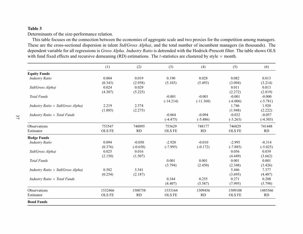
Table 3

Determinants of the size-performance relation.

This table focuses on the connection between the economies of aggregate scale and two proxies for the competition among managers.

These are the cross-sectional dispersion in talent Std(Gross Alpha), and the total number of incumbent managers (in thousands). The

dependent variable for all regressions is Gross Alpha. Industry Ratio is detrended with the Hodrick-Prescott filter. The table shows OLS

with fund fixed effects and recursive demeaning (RD) estimations. The t-statistics are clustered by style × month.

(1) (2) (3) (4) (5) (6)

Equity Funds

Industry Ratio 0.004 0.019 0.190 0.028 0.082 0.013

(0.343) (2.958) (5.103) (5.493) (3.094) (3.214)

Std(Gross Alpha) 0.024 0.029 0.011 0.013

(4.307) (5.225) (2.272) (2.819)

Total Funds -0.001 -0.001 -0.001 -0.000

(-14.214) (-11.368) (-6.006) (-5.781)

Industry Ratio × Std(Gross Alpha) 2.219 2.574 1.746 1.920

(1.885) (2.275) (1.948) (2.222)

Industry Ratio × Total Funds -0.064 -0.094 -0.032 -0.057

(-4.475) (-5.486) (-3.263) (-4.303)

Observations 753547 748095 753629 748177 746829 741448

Estimator OLS FE RD OLS FE RD OLS FE RD

Hedge Funds

Industry Ratio 0.094 -0.050 -2.920 -0.010 -2.995 -0.314

(0.376) (-0.658) (-7.995) (-0.172) (-7.885) (-5.025)

Std(Gross Alpha) 0.025 0.016 0.056 0.039

(2.150) (1.507) (4.449) (3.662)

Total Funds 0.001 0.001 0.001 0.001

(3.794) (2.450) (2.348) (3.426)

Industry Ratio × Std(Gross Alpha) 0.582 5.541 5.446 7.377

(0.254) (2.187) (3.695) (4.487)

Industry Ratio × Total Funds 0.344 0.255 0.271 0.208

(8.407) (5.587) (7.995) (5.798)

Observations 1532466 1508758 1533164 1509456 1509108 1485566

Estimator OLS FE RD OLS FE RD OLS FE RD

Bond Funds

37

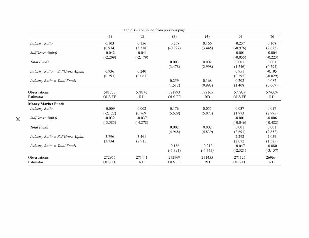
Table 3 – continued from previous page

(1) (2) (3) (4) (5) (6)

Industry Ratio 0.103 0.156 -0.258 0.166 -0.257 0.108

(0.974) (3.338) (-0.927) (3.445) (-0.976) (2.672)

Std(Gross Alpha) -0.042 -0.041 -0.001 -0.004

(-2.209) (-2.179) (-0.055) (-0.223)

Total Funds 0.003 0.002 0.001 0.001

(3.478) (2.998) (1.246) (0.794)

Industry Ratio × Std(Gross Alpha) 0.936 0.240 0.951 -0.105

(0.293) (0.067) (0.295) (-0.029)

Industry Ratio × Total Funds 0.259 0.168 0.202 0.087

(1.512) (0.993) (1.408) (0.667)

Observations 581773 578145 581793 578165 577939 574324

Estimator OLS FE RD OLS FE RD OLS FE RD

Money Market Funds

Industry Ratio -0.009 0.002 0.176 0.055 0.037 0.017

(-2.122) (0.769) (5.529) (5.073) (1.973) (2.995)

Std(Gross Alpha) -0.032 -0.037 -0.001 -0.006

(-3.585) (-4.278) (-0.046) (-0.482)

Total Funds 0.002 0.002 0.001 0.001

(4.948) (4.839) (2.691) (2.852)

Industry Ratio × Std(Gross Alpha) 3.796 3.461 2.292 2.059

(3.734) (2.911) (2.072) (1.585)

Industry Ratio × Total Funds -0.186 -0.212 -0.047 -0.080

(-5.391) (-4.745) (-2.321) (-3.157)

Observations 272955 271441 272969 271455 271125 269634

Estimator OLS FE RD OLS FE RD OLS FE RD

38

Table 4

Evolution of the economies of scale for equity mutual funds.

This table shows multiple snapshots over time of the relation between returns and size for equity mutual funds. Each panel is similar

to the first panel in Table 2, but with the sample restricted to dates until December of the cutoff year. The first year in the sample for all

regressions is 1985. The controls that are not shown are the lagged values of Gross Alpha, the percentage growth in the number of funds

Fund Growth, and Fund Age (in years). The table shows OLS with fund fixed effects and recursive demeaning (RD) estimations. The

t-statistics are clustered by style × month.

(1) (2) (3) (4) (5) (6)

Year cutoff: 1990

Fund Size -7.038e-08 -4.412e-07 -5.173e-08 -3.948e-07

(-0.902) (-9.618) (-0.861) (-5.867)

Industry Ratio -0.0403 -0.0119 0.0862 -0.0083

(-0.999) (-4.668) (1.980) (-1.840)

Observations 45136 44622 45165 45119 44237 44193

Number of Funds 917 917 917 917 917 917

Controls No No No No Yes Yes

Estimator OLS FE RD OLS FE RD OLS FE RD

Year cutoff: 1995

Fund Size 3.982e-09 1.655e-06 2.838e-08 5.826e-07

(0.332) (1.922) (2.641) (3.134)

Industry Ratio -0.0139 -0.0127 0.0337 0.0048

(-2.517) (-8.372) (2.611) (1.667)

Observations 111532 110456 111566 111332 109850 109619

Number of Funds 1704 1704 1704 1704 1704 1704

Controls No No No No Yes Yes

Estimator OLS FE RD OLS FE RD OLS FE RD

Year cutoff: 2000

Fund Size 6.899e-09 4.193e-07 3.868e-08 1.989e-07

(0.863) (11.259) (4.987) (8.951)

Industry Ratio -0.0165 -0.0167 0.0252 -0.0013

(-6.104) (-11.276) (2.304) (-0.587)

Observations 228290 225993 228369 227793 225126 224557

Continued on next page

39

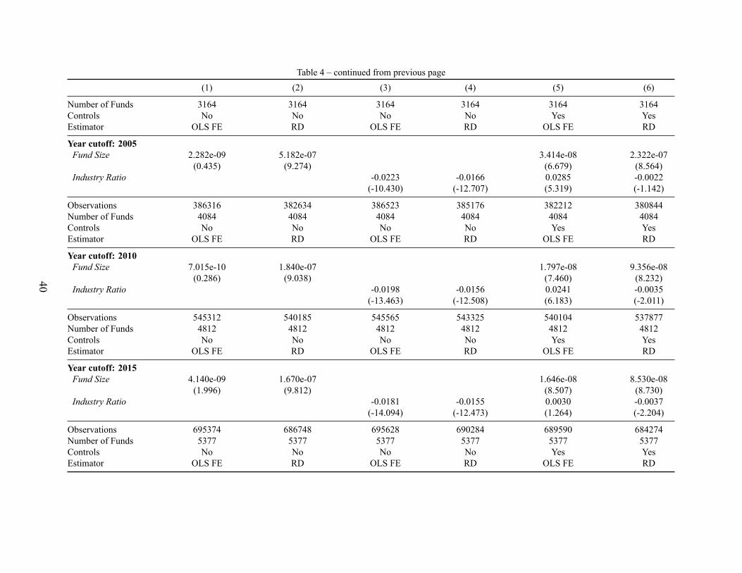
Table 4 – continued from previous page

(1) (2) (3) (4) (5) (6)

Number of Funds 3164 3164 3164 3164 3164 3164

Controls No No No No Yes Yes

Estimator OLS FE RD OLS FE RD OLS FE RD

Year cutoff: 2005

Fund Size 2.282e-09 5.182e-07 3.414e-08 2.322e-07

(0.435) (9.274) (6.679) (8.564)

Industry Ratio -0.0223 -0.0166 0.0285 -0.0022

(-10.430) (-12.707) (5.319) (-1.142)

Observations 386316 382634 386523 385176 382212 380844

Number of Funds 4084 4084 4084 4084 4084 4084

Controls No No No No Yes Yes

Estimator OLS FE RD OLS FE RD OLS FE RD

Year cutoff: 2010

Fund Size 7.015e-10 1.840e-07 1.797e-08 9.356e-08

(0.286) (9.038) (7.460) (8.232)

Industry Ratio -0.0198 -0.0156 0.0241 -0.0035

(-13.463) (-12.508) (6.183) (-2.011)

Observations 545312 540185 545565 543325 540104 537877

Number of Funds 4812 4812 4812 4812 4812 4812

Controls No No No No Yes Yes

Estimator OLS FE RD OLS FE RD OLS FE RD

Year cutoff: 2015

Fund Size 4.140e-09 1.670e-07 1.646e-08 8.530e-08

(1.996) (9.812) (8.507) (8.730)

Industry Ratio -0.0181 -0.0155 0.0030 -0.0037

(-14.094) (-12.473) (1.264) (-2.204)

Observations 695374 686748 695628 690284 689590 684274

Number of Funds 5377 5377 5377 5377 5377 5377

Controls No No No No Yes Yes

Estimator OLS FE RD OLS FE RD OLS FE RD

40

Table 5

Frequency table for investment styles.

Frequency Percent Cumulative Percent

Equity Funds

Cap-based 177374 22.91 22.91

Growth 333415 43.06 65.97

Growth and Income 188455 24.34 90.31

Sector 75021 9.69 100.00

Total 774265 100.00

Index Funds

Equity 47024 76.71 76.71

Fixed Income 14276 23.29 100.00

Total 61300 100.00

ETFs

Equity 63959 73.04 73.04

Fixed Income 23609 26.96 100.00

Total 87568 100.00

Hedge Funds

Arbitrage 327547 20.62 20.62

Emerging Markets 198069 12.47 33.08

Hedging 621222 39.10 72.18

Macro 178109 11.21 83.39

Market Neutral 40860 2.57 85.97

Multistrategy 175001 11.01 96.98

Unknown 47979 3.02 100.00

Total 1588787 100.00

Bond Funds

Corporate 87664 14.84 14.84

Generic 170140 28.80 43.63

Government 85415 14.46 58.09

Municipal 247608 41.91 100.00

Total 590827 100.00

Money Market Funds

Government 88207 30.66 30.66

Municipal 108758 37.81 68.47

Prime 90704 31.53 100.00

Total 287669 100.00

41

Table 6

Comparison between industry and style-wide size ratios.

This table is the same as Table 2, but with Fund Size replaced by Style Ratio. The latter is the aggregate size within an investment style

divided by the relevant total market capitalization (US stock market for ETFs, equity, hedge, and index funds; US debt market for bond

and money market funds). The table shows OLS with fund fixed effects and recursive demeaning (RD) estimations. The t-statistics areclustered by style × month.

(1) (2) (3) (4) (5) (6)

Equity Funds

Style Ratio -0.0211 -0.0295 0.0168 0.0241

(-9.424) (-9.513) (4.009) (3.838)

Industry Ratio -0.0142 -0.0137 -0.0186 -0.0218

(-13.210) (-12.020) (-10.198) (-9.223)

Observations 753628 748176 753629 748177 753628 748176

Estimator OLS FE RD OLS FE RD OLS FE RD

Index Funds

Style Ratio -0.4552 -0.3435 -0.9554 -0.8246

(-1.373) (-0.606) (-1.808) (-0.798)

Industry Ratio -0.2324 -0.1766 0.4152 0.3406

(-0.976) (-0.521) (1.158) (0.708)

Observations 60599 60109 60600 60110 60599 60109

Estimator OLS FE RD OLS FE RD OLS FE RD

ETFs

Style Ratio -0.0158 0.0520 -0.3121 -0.3787

(-0.036) (0.071) (-0.605) (-0.316)

Industry Ratio 0.0163 0.0666 0.2264 0.3008

(0.052) (0.154) (0.647) (0.626)

Observations 86676 85496 86676 85496 86676 85496

Estimator OLS FE RD OLS FE RD OLS FE RD

Hedge Funds

Style Ratio 0.3053 0.1748 0.0498 0.0060

(5.479) (3.085) (0.414) (0.048)

Industry Ratio 0.0858 0.0505 0.0748 0.0492

(6.171) (3.870) (2.501) (1.685)

42

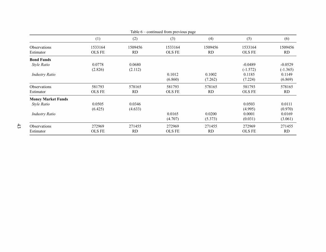
Table 6 – continued from previous page

(1) (2) (3) (4) (5) (6)

Observations 1533164 1509456 1533164 1509456 1533164 1509456

Estimator OLS FE RD OLS FE RD OLS FE RD

Bond Funds

Style Ratio 0.0778 0.0680 -0.0489 -0.0529

(2.826) (2.112) (-1.572) (-1.365)

Industry Ratio 0.1012 0.1002 0.1185 0.1149

(6.860) (7.262) (7.224) (6.869)

Observations 581793 578165 581793 578165 581793 578165

Estimator OLS FE RD OLS FE RD OLS FE RD

Money Market Funds

Style Ratio 0.0505 0.0346 0.0503 0.0111

(6.425) (4.633) (4.995) (0.970)

Industry Ratio 0.0165 0.0200 0.0001 0.0169

(4.707) (5.373) (0.031) (3.061)

Observations 272969 271455 272969 271455 272969 271455

Estimator OLS FE RD OLS FE RD OLS FE RD

43