ECONOMICS

THE ROTTERDAM DEMAND MODEL HALF A CENTURY ON

by

Kenneth W Clements Business School

University of Western Australia

and

Grace Gao Bankwest Curtin Economics Centre

Curtin University

DISCUSSION PAPER 14.34

December 2014 THE ROTTERDAM DEMAND MODEL

HALF A CENTURY ON∗

by

Kenneth W Clements Business School

The University of Western Australia

and

Grace Gao Bankwest Curtin Economics Centre

Curtin University

DISCUSSION PAPER 14.34

Abstract Half a century ago, Barten (1964) and Theil (1965) formulated what is now known as

the Rotterdam model. A path-breaking innovation, this system of demand equations allowed

for the first time rigorous testing of the theory of the utility-maximising consumer. This has

led to a vibrant, on-going strand of research on the theoretical underpinnings of the model,

extensions and numerous applications. But perhaps due to its European heritage and

unorthodox derivation, there is still misunderstanding and a tendency for the Rotterdam

model to be regarded with reservations and/or uncertainties (if not mistrust). This paper

marks the golden jubilee of the model by clarifying its economic foundations, highlighting its

strengths and weaknesses, elucidating its links with other models of consumer demand, and

dealing with some recent developments that have their roots in Barten and Theil’s pioneering

research of the 1960s.

∗ We would like to thank Paul Frijters for helpful comments and Aiden Depiazzi, Haiyan Liu and Jiawei Si for excellent research assistance. This research was financed in part by the ARC and BHP Billiton.

1. INTRODUCTION

Few papers in economics have a working life, in terms of citations and influence, longer than

a decade or so. It is thus a very rare event for a paper to continue to be read, cited, taught and

followed after almost half a century. Two such papers are Anton Barton’s “Consumer Demand

Equations Under Conditions of Almost Additive Preferences” and Henri Theil’s “The Information

Approach to Demand Analysis” that were published in Econometrica in 1964 and 1965, respectively

(Barten, 1964, Theil, 1965). These related papers introduced what has become known as the

“Rotterdam model”. For the first time, this model combined generality and operational tractability so

that it became a prominent vehicle for the econometric analysis of the pattern of consumer demand

and the rigorous testing of utility-maximisation theory. To this day, the model still appears in leading

journals, and the general approach has formed the basis for a rich class of models known as the

“differential approach” to demand analysis that is used in both time-series and cross-country

contexts. The Rotterdam model has spawned an extensive literature and occupies a similar status in

consumer demand to the linear expenditure system (LES, Stone, 1954), the translog (Christensen et

al., 1975) and the almost ideal demand system (Deaton and Muellbauer, 1980a). Figure 1 provides

some evidence for this claim in terms of citations.

The beguilingly simplicity, transparency and apparent generality of the Rotterdam model

have led to its prominent position in demand analysis. Interestingly (ironically?), these very features

have led to controversy, misunderstanding and a feeling that perhaps the Rotterdam system was “too

good to be true” and its simplicity deceptive. Non-Rotterdam approaches such as the LES start with

the algebraic form of the consumer’s utility function and then derive the corresponding demand

functions, which obviously contain (most of) the information embodied in the utility function. This

sequence is reversed in the Rotterdam approach. It starts with demand functions, takes the total

differential, uses utility-maximisation theory to give restrictions on the demand functions and then,

as the last step, takes certain transformations of the slopes of the demand functions to be constants.

The important distinction is that the utility function is not specified explicitly, but lies behind the

demand equations in the background. Preferences are not ignored as the utility function provides

restrictions on (transforms of) the slopes of the demand equations. In this sense, the Rotterdam

system can be considered to be consistent with a variety of utility functions.

As the underlying theory can confront the data only via demand functions, there is the merit

in directness in the Rotterdam approach that starts and ends with demand functions. Expressing the

consumer’s preferences in the form of the utility function or the cost function involves a construct

that is unobservable; in this sense, competitive approaches that start by specifying preferences are

1

indirect in the theory-data matching process. A related issue is the question of parameterisation of

the Rotterdam, which contains a mixture of constant slopes of Engel functions and a type of semi-

elasticity for the prices. This formulation is unconventional and has been the source of some

difficulties and resistance. For the non-Rotterdam approaches the question of parameterisation is

simple: Choose the algebraic form of the utility function (direct or indirect, or the cost function),

which then determines the form of the corresponding demand equations. The reverse engineering

methodology makes the Rotterdam appear different and distinct and, arguably, is at the heart of the

controversy and misunderstanding. Rotterdam critics also argue the microeconomic foundations of

the model are questionable and have claimed it implies Cobb-Douglas preferences, so that all income

elasticities are unity and price elasticities are -1, which, if true, would be a devastating weakness.

Why does the Rotterdam model continue to be enthusiastically used and endure in view of

such apparent trenchant criticism? Some of the controversy will possibly never be completely settled,

and, of course, it is not productive to be dogmatic in matters that are inherently unresolvable if they

simply reflect different preferences (of researchers). The fact is the Rotterdam passes the Darwinian

test of survival by a sizable margin, and it seems it will continue to be used for some time in the

future. It is thus appropriate to mark the first half century of the Rotterdam model’s existence with a

review that sets out the model, its advantages and disadvantages and reveals its surprisingly close

links with other popular models, with the objective of clarifying at least some of the

misunderstanding that still surrounds the model. Relatedly, it is also appropriate to discuss the

developments that the Rotterdam directly lead to – the differential approach and the emerging area of

cross-county demand analysis.

2. THE ORIGINAL FORMULATION

This section presents the original foundation and formulation of the Rotterdam model by

Barten (1964) and Theil (1965). In the interests of focusing on what is important and making it as

accessible as possible, the presentation is selective and gives a simplified exposition of the original

papers. Two additional “basic sources” are Theil (1967, Chap 5-6) and Theil (1975/76).1

Basic Concepts

Let ip and iq be the price and quantity demanded of good i, i 1, , n.= The consumer is

taken to choose the basket 1 nq , ,q to maximise the utility function

(2.1) ( )1 nu q , ,q

1 For reviews of the broader area of applied demand analysis, see Barnett and Serletis (2008), Barten (1977), Bewley (1986). Blundell (1988), Brown and Deaton (1972), Deaton (1986), Deaton and Muellbauer (1980b), Goldberger (1987), Phlips (1974), Pollak and Wales (1992), Powell (1974), Theil (1980) and Theil and Clements (1987).

2

subject to the budget constraint

(2.2) n

i ii 1

M p q ,=

= ∑

where M is total expenditure (“income” for short). This leads to a demand equation for good i of the

form ( )i i 1 nq q M,p , , p .= As money income is held constant, this is a Marshallian demand

equation. The differential of this demand equation is n

i ii j

j 1 j

q qdq dM dp .M p=

∂ ∂= +

∂ ∂∑

The total effect on the consumption of good i of a change in the price of good j i jq p ,∂ ∂ can be

decomposed into income and substitution effects according to the Slutsky equation,

i j ij j iq p s q q M ,∂ ∂ = − ∂ ∂ where ijs is the substitution effect that holds real income constant. Thus,

the above can be expressed as

n ni

i j j ij jj 1 j 1

qdq dM q dp s dp .M = =

∂= − + ∂

∑ ∑

The term in brackets is the change in money income deflated of the income effects of the n price

changes, which represents the change in real income. Using the identity ( )d log x dx x,= the above

can be expressed logarithmically as

(2.3) ( ) ( ) ( ) ( )n n

j j jii j ij j

j 1 j 1i i

p q pM qd logq d log M d log p s d log p .q M M q= =

∂= − + ∂

∑ ∑

To simplify the above, let ( ) ( ) ( )( )i i i ilog q log M M q q Mη = ∂ ∂ = ∂ ∂ be the income

elasticity of good i, ( ) ( ) ( )ij i j j i ijlog q log p p q sη = ∂ ∂ = be the ( )thi, j price elasticity (income

compensated), j j jw p q M= the budget share of j and ( ) ( ) ( )nj 1 j jd log Q d log M w d log p== − Σ be the

change in real income. Using these concepts, equation (2.3) then becomes

(2.4) ( ) ( ) ( )n

i i ij jj 1

d log q d log Q d log p .=

= η + η∑

For i 1, , n,= (2.4) is a system of n demand equations, the parameters of which satisfy the adding-

up constraints

(2.5) n n

i i i iji 1 i 1

w 1, w 0, j = 1, ,n, = =

η = η =∑ ∑

3

which follow from the budget constraint (2.2). As real income is controlled for in equation (2.4),

demand homogeneity means that an equiproportional increase in all prices has no effect on quantities

consumed, which implies

(2.6) n

ijj 1

0, i 1, ,n. =

η = =∑

Finally, Slutsky symmetry states that the substitution effects are symmetric in i and j, that is,

ij jis s , i, j 1, , n.= = As ( )ij j i ijp q s ,η = symmetry in terms of elasticities takes the form

( ) ( )i j ij j i jiq p q p ,η = η or, multiplying by i jp p M ,

(2.7) i ij j jiw w , i, j 1, , n.η = η =

Transforming Log-Linear Demands

To apply model (2.4) to time-series data, Barten (1964) replaces infinitesimal changes with

finite changes and takes the elasticities to be constants:

(2.8) n

it i t ij jt itj 1

Dq DQ Dp ,=

= η + η + ε∑ i 1, , n goods, t 1, ,T observations,= =

where D denotes the log-change operator ( )t t t 1Dx log x log x −= − and itε is a disturbance term. This

is an n-equation system that is linear in the parameters, the elasticities. Furthermore, the

homogeneity constraint (2.6) is also linear. These are attractive features of the model, and Barten

(1964, p. 8) justifies its use “for reasons that are largely pragmatic”. Not so attractive is the

appearance of the budget shares in constraints (2.5) and (2.7). Barten (1964) treats the shares as

constants in these constraints and replaces them with their sample means.

Theil (1965) dealt with this difficulty by multiplying both sides of (2.8) by the budget share

and then reparameterising. As the model refers to changes over time from period t-1 to t, the share in

either of these periods would seem to have equal merits. But to choose one leads to an asymmetry

that is best avoided. To treat both periods symmetrically, Theil (1965) proposed a two-period moving

average of the share over t-1, t, ( )it i,t 1 itw 1 / 2 w w .−= + The reformulated version of (2.8) is

(2.9) n

it it i t ij jt itj 1

w Dq DQ Dp ,=

= q + p + µ∑ i 1, , n goods, t 1, ,T observations,= =

4

The new parameters are i it iwq = η and ij it ijw ,p = η which are taken to be constants, while i it itwµ = ε

is the new disturbance. Thus, we move from a constant elasticity formulation to something else; that

something else, model (2.9), has come to be known as the Rotterdam model.2

Interpretations and Implications

The Rotterdam model describes the budget-share weighted change in the quantity consumed

of good i, it itw Dq , as a linear function of the change in real income, tDQ , and the change in each of

the n prices, 1t ntDp , ,Dp . There is one equation for each good, so (2.9) comprises a system of n

equations; and this system refers to the changes over successive periods for each of T periods. The

parameters of the model are i ij, i 1, , n, and , i, j 1, , n,q = p = which have the following

interpretations. As the budget share is defined as i i iw p q M= and as the income elasticity is

( )( )i i iM q q M ,η = ∂ ∂ it follows that their product i iw η is ( )i i i ip q M p q M.∂ ∂ = ∂ ∂ Thus, the

parameter attached to the real income variable in (2.9), i ,q is just this product, so it follows that

( )i i ip q M.q = ∂ ∂ Accordingly, iq answers the question, if income rises by one dollar, how much of

this is spent on good i? This parameter is known as the marginal share of good i. An inferior good

has a negative marginal share, while for a normal good the share is positive. As the additional

income is taken to be completely spent, the marginal shares have a unit sum:

(2.10) n

ii 1

1.=

q =∑

The income elasticity of good i implied by model (2.9) is simply the ratio of the marginal

share to its budget share, i i iw ,η = q so that luxuries ( )i 1η > have a marginal share greater than the

budget share and vice versa for necessities ( )i 1 .η < Constraint (2.10) implies that a budget-share

weighted average of the income elasticities is unity, which is the first member of (2.5). It can be seen

that one of the attractions of taking the marginal shares to be constants is that one of the adding-up

constraints is satisfied as a parametric restriction without any reference to the (variable) budget

shares.

2 The name, introduced by Parks (1969), reflects the location of Barten and Theil when the model was first formulated. Theil moved from The Netherlands School of Economics (now Erasmus University Rotterdam) to The University of Chicago in 1966, then in 1981, to The University of Florida, Gainesville and retired in 1994. He died in 2000. Barten, Theil’s former student, moved from Rotterdam to The Catholic University of Louvain and then later to Tilburg University. For biographical information on these two pioneers of econometrics, see Barnett (2003), Bewley (2000), Blaug (1999), Koerts (1992), Raj (1992) and Seale and Moss (2003).

5

Next, consider the coefficients of the prices in (2.9). The coefficient of the change in the thj

price in the thi equation is ij.p As this is the product of the budget share of i, itw , and the ( )thi, j

price elasticity, ij ,η it follows that the Rotterdam model (2.9) implies that this price elasticity takes

the form ij ij itw .η = p Multiplying both sides of the homogeneity constraint (2.6) by itw gives

(2.11) n

ijj 1

0, i 1, , n. =

p = = …∑

Similarly, the symmetry constraints (2.7) now become

(2.12) ij ji , i, j 1, , n.p = p =

As ijp refers to the substitution effect of a change in the price of good j on the demand for good i

when real income is held constant, ijp is known as the ( )thi, j Slutsky coefficient. As can be seen, the

Rotterdam specification solves the problem with the budget shares being part of the constraints of the

constant elasticity model (2.8). The issue not yet discussed is the second member of (2.5). But as

now will be shown, with the Rotterdam, this also becomes a simple matter.

The consumer’s budget is given by equation (2.2). The differential is

( )ni 1 i i i idM p dq q dp ,== Σ + or ( ) ( ) ( )d log M d log Q d log P ,= + with

( ) ( )n

i ii 1

d logQ w d logq=

= ∑ and ( ) ( )n

i ii 1

d log P w d log p=

= ∑

the Divisia volume and price indexes. A frequently employed discrete approximation of this volume

index is

(2.13) n

t it iti 1

DQ w Dq .=

= ∑

The Rotterdam model uses this index to measure the change in real income, which is the reason for

using the notation tDQ in both (2.9) and (2.13). This means if we add both sides of equation (2.9)

over i 1, , n,= we obtain tDQ on the left-hand side. To ensure that the right-hand side is also

tDQ , we need the cross-equation restrictions on the parameters given by (2.10) and

(2.14) n

iji 1

0,=

p =∑ j 1, , n,=

6

as well the disturbances having a zero sum, ni 1 it 0.=Σ µ = Constraint (2.14) coincides with the second

member of (2.5), ni 1 i ijw 0, j 1, , n.=Σ η = = The vanishing of the budget shares here again underscores

the attractiveness of the Rotterdam formulation.3

As mentioned above, the dependent variable of the model, it itw Dq , is a budget-share

weighted change in the quantity consumed of good i. Something more can be said about the

interpretation of this variable. First, from equation (2.13), it itw Dq is the contribution of good i to the

change in real income. A second interpretation derives from the differential of the budget share,

( ) ( ) ( )i i i i i idw w d logq w d log p w d log M ,= + − which shows that the change in the share is made up

of price, quantity and income components. If for the transition from period t-1 to t, this is

approximated by it i,t 1 it it it it it tw w w Dq w Dp w DM ,−− ≈ + − it can then be seen that the dependent

variable of the model is also interpreted as the quantity component of the change in the budget share

of good i.

Further Issues

The above presentation of the Rotterdam model emphasises its interpretation and the

simplicity of the constraints on the parameters. These features have contributed to its widespread use,

as well as some of the controversy surrounding the model, to be discussed in the next section. But

before concluding this section, there are other aspects of Rotterdam that should be at least

mentioned. One is the extensive econometric analysis that has been developed to estimate and test

the model. As model (2.9) is linear in the parameters, when income and the prices are taken as

exogenous it can be estimated as a seemingly unrelated regression system. Moreover, as the

homogeneity and symmetry constraints are also linear, their testing would also seem to be

straightforward. But as Laitinen (1978) and Meisner (1979) showed with Monte Carlo studies, the

conventional tests based on asymptotic theory (that is, as T )→ ∞ break down when the number of

goods n is large relative to the number of time periods, but these tests can be modified

appropriately.4

The structure of preferences within the Rotterdam framework should also be mentioned. The

consumer’s preferences are described by the utility function (2.1). If this general form is made more

3 Defining real income as the sum of the left-hand variables means that model (2.9) is an allocation system. That is, given the price changes and the values of the disturbances, the n equations of the model allocate the change in real income to each of the n goods. Knowledge of n-1 allocations is sufficient to determine that of the th ;n in other words, the Rotterdam model is a singular system in which one equation is redundant. This means that the adding up constraints are automatically satisfied and not testable. 4 For a comprehensive account of these matters, see Theil (1987).

7

specific there are additional restrictions on the demand equations. We could, for example, suppose

that the n goods are unrelated in the sense that the marginal utility of each good is independent of the

consumption of all others. This means that ( ) ( )n1 n i 1 i iu q , ,q u q ,== Σ where ( )i iu q is the thi sub-

utility function that involves only iq . This case is known as preference independence (or strong

separability) and, as discussed in Section 4, the ( )thi, j price elasticity takes the form

( )ii i i i1 wη = φη − η if i j= (denoting the own-price elasticity) and ij i j jwη = −φη η if i j≠ (the cross-

price elasticity), where 0φ < is a factor of proportionality (known as the “income flexibility”, the

reciprocal of the income elasticity of the marginal utility of income), iw is the budget share of good i

and iη is the income elasticity of i. Defining ijδ as the Kronecker delta ( )ij 1 if i j, 0 otherwiseδ = =

and using ij i ijw ,p = η the substitution effect in (2.9) then becomes

(2.15) ( ) ( ) ( )n n n

ij jt i i ij j j jt i ij j jt i it tj 1 j 1 j 1

Dp w w Dp Dp Dp DP ,= = =

′p = φ η δ − η = φq δ − q = φq −∑ ∑ ∑

where ni iti 1DP Dp=′ = q∑ is the Frisch (1932) price index.

Thus, the preference independence version of model (2.9) takes the form

(2.16) ( )it it i t i it t itw Dq DQ Dp DP .′= q + φq − + µ

The term in brackets in this equation is the change in the relative price of good i, with the Frisch

index acting as a deflator of the change in the nominal price. Accordingly, under preference

independence, consumption of good i depends on income and its own relative price, not the prices of

the other goods. In words, the absence of any cross effects in the utility function translates directly

into the absence of cross-price effects in the demand equations. It follows from equation (2.15) that

the preference independence hypothesis takes the form of simple parametric restrictions on the

Slutsky coefficients: ( )ij i ij j ,p = φq δ − q for i, j 1, , n.=

As preference independence rules out all utility interactions among goods, this condition is

strong and is often thought to be more applicable to the broad aggregates such as food, clothing,

housing, etc., where the substitution possibilities are likely to be modest. But as it is the simplest

form of preferences, it is a natural starting point for testing. According to the weaker condition of

block independence (or weak separability), groups of goods are additive in the utility function, rather

than individual goods. This leads to group demand equations and systems of conditional demands,

which express the demand for each member of a group in terms of the total consumption of the group

and prices within the group. An example is the alcoholic beverages group comprising beer, wine and

spirits. When alcohol is block independent, there exists a group demand for alcohol as a whole, 8

which depends on real income and the price of alcohol. Then, given the demand for total alcohol,

there is a system of three conditional demand equations. The linear structure of the Rotterdam

framework means that the group demands and conditional demands have the same basic Rotterdam

forms and are consistent in aggregation. Conditional demand equations allow the focus to be on sub-

groups of goods that are of particular interest. Block independence implies parametric restrictions on

the Slutsky coefficients that are analogous to those of preference independence. Thus, the Rotterdam

model allows ideas regarding the nature of goods, and how closely related goods might be grouped

together, to be mapped straightforwardly into observed demand behaviour via simple parametric

restrictions.

3. CRITICISMS

Like all models, the Rotterdam system can at best be considered as only an approximation to

reality and is not perfect. In this section we consider three criticisms of the Rotterdam model.

Constant Marginal Shares

The infinitesimal version of equation (2.9) is ( ) ( ) ( )ni i i ij jj 1w d logq d logQ d log p .== q + p∑ If

prices are held constant, then the substitution term vanishes and ( ) ( )i i iw d logq d logQ .= q As the

change in real income ( )d logQ coincides with the change in money income ( )d log M , this

becomes ( ) ( )i i iw d logq d log M ,= q or i i ip dq dM.= q Integration yields a linear Engel curve:

(3.1) i i i ip q M,= α + q

where iα is a constant of integration. By definition, the income elasticity of i is

(3.2) ( )( )

( )i i ii i i ii

i i i

logq p q Mq q p q M ,log M M M p q M w

∂ ∂ ∂∂ ∂ ∂η = = = =

∂ ∂

where the last step follows when the price is held constant and where i i iw p q M= is the budget

share of i, as before. Equation (3.2) shows that the income elasticity is the ratio of the marginal share

to the corresponding budget share; geometrically, the elasticity is the ratio of the slope of the Engel

curve to that of the ray from the origin. Thus, for the linear Engel curve (3.1) that is implied by the

Rotterdam model, the elasticity takes the form i i iw ,η = q with the marginal share, i ,q a constant.

The constant marginal share means that the income elasticity is inversely proportional to the

budget share, that is ( ) ( )i id log d log w .η = − If the price is held constant, it follows from

i i iw p q M= and equation (3.2) that

9

(3.3) ( ) ( ) ( ) ( ) ( )i i id log w d logq d log M 1 d log M ,= − = η −

so that

(3.4) ( ) ( ) ( )i id log 1 d log M .η = − η −

This shows that when the marginal share is constant, the income elasticity of the income elasticity is

( )i 1 .− η − Accordingly, for luxuries ( )i 1η > , income growth causes the income elasticity to fall,

while the reverse is true for necessities. This type of behaviour is problematic for food, the leading

necessity, as it means that its income elasticity for the rich is larger than that for the poor: Food is

less of a necessity, or more of a luxury, for a more affluent consumer! This makes no economic sense

and is contradicted by several studies.5

Fortunately, a simple modification to the Rotterdam model solves the problem: Working’s

(1943) model states that the budget share is a linear function of the logarithm of income:

(3.5) i i iw log M,= α + β

where iα and iβ are new parameters.6 The implied marginal share is

(3.6) ( )i i

i i

p qw .

M∂

= + β∂

Rather than being a constant, now the marginal share differs from the corresponding budget share by

a constant, i.β The income elasticity is

(3.7) ii

i

1 ,wβ

η = +

so that the good is a luxury (necessity) if its i 0 ( 0).β > < The differential of (3.7) can be expressed as

( ) ( ) ( )i i i id log 1 d log w ,η = − η − η so that, in view of (3.3),

(3.8) ( ) ( ) ( )2

ii

i

1d log d log M .

η −η = −

η

Now, the income elasticity always falls as income grows (as long as i 0)η > : The food income

elasticity for the rich is now lower than that for the poor, which solves the previous problem.

5 Gao (2012) uses the 2005 ICP data for a large number of countries to provide evidence on this matter by plotting the log of the food budget share (w) against the log of income (M). There is clear evidence of a downward-sloping relationship that gets steeper as income rises. As ( ) ( )log w log M 1,∂ ∂ = η − where η is the food income elasticity, the negative slope means that 1,η < while the increasing slope means that η falls as income rises. For other evidence that η declines with income, see, e. g., Clements and S. Selvanathan (1994), Deaton and Paxson (1998), Hymans and Shapiro (1976), Lluch et al. (1977) and Timmer and Alderman (1979). 6 This model is also associated with Leser (1963).

10

The income term in the Rotterdam model (2.9) is i tDQq where i constant.q = Alternatively,

if we use the variable marginal share implied by Working’s model, (3.6), the income term then

becomes ( )it i tw DQ+ β , where to be consistent with the left-hand-side of Rotterdam, itw is used.

Then, after minor rearrangements, the demand equation for good i takes the form

( )n

it it t i t ij jt itj 1

w Dq DQ DQ Dp ,=

− = β + p + µ∑

where i ,β the coefficient of income, has exactly the same interpretation of iβ in Working’s model.

This shows that the Rotterdam model can be modified in a simple manner to make the income

responses more satisfactory.

What’s Constant, What’s Variable?

The thi equation of the Rotterdam model is nit it i t j 1 ij jt itw Dq DQ Dp .== q + Σ p + µ Here, the

quantity component of the change in the thi budget share is a linear function of the change in real

income, the n price log-changes and a random disturbance term. The constant parameters are the

good’s marginal share, i ,q and the Slutsky coefficients, ij , j 1, , n,p = defined as

(3.9) ( ) i ji i ii ij ij ij

j DQ 0

p pp q q, s , with s .M M p

=

∂ ∂q = p = ⋅ =

∂ ∂

These expressions have been the source of some confusion: At first glance, they look complex as

they involve derivatives of the demand function, as well as prices and income. If the derivatives are

constant, while prices and income are variable, how can the terms in equation (3.9) possibly be

constant parameters?

Clearly, iq and ijp cannot be constants if one insists on constant derivatives. It may be

common practice to think of derivatives as being more or less constant, but this is just a matter of

convenience that serves as a simplification, when, for example, comparative statics is used to

determine a sign. But there is no fundamental reason for these derivatives to be constants. The issue

is the choice of the functional form of the equation to be estimated. Take again the case of the Engel

curve for good i: We could consider the two alternatives, the linear specification (3.1) or a double-

log form,

( )i i i i i i i ip q M, log p q log M.′ ′= α + β = α + β

11

This involves choosing between specifying a constant slope, i ,β or a constant elasticity, i .′β If the

slope is constant, then elasticity is variable, and vice versa, as ( )i i i iM p q .′β = β ⋅ The goodness of fit

of the two specifications is the obvious way to choose between them.7

The Slutsky coefficient ijp in equation (3.9) involves prices, income and preferences in the

form of the response to the thj price when the consumer remains on the same indifference curve.8 An

objection to treating ijp as a constant is that this mixture of the subjective (preferences) and the

objective (prices and income) is somehow mixed up. This point has been heard (but apparently not

written down) at The University of Chicago and possibly reflects the influence of Milton Friedman,

who forcefully argued that preferences are distinct from the budget constraint and those who mix the

two do so at their peril. While this is no doubt a good guiding principle of applied price theory, the

objection has little merit in the context of the Rotterdam model which is used for applied demand

analysis. In essence, this is similar to the issue discussed above parameterisation on the basis of

goodness-of-fit considerations.

The variable on the left-hand side of the Rotterdam equation (2.9) is it itw Dq . Thus, if we set

the disturbance term in that equation at its expected value of zero and then divide both sides by the

budget share, we obtain a demand equation with the quantity change on the left:

n n

ijiit t jt it t ijt jt

j 1 j 1it it

Dq DQ Dp DQ Dp ,w w= =

p q= + = η ⋅ + η ⋅

∑ ∑

where it i itwη = q is the income elasticity of demand for good i and ijt ij itwη = p is the ( )thi, j

compensated price elasticity. In this form, it is clear that the Rotterdam approach leads to income and

price elasticities that are variable. These elasticities always satisfy the adding-up constraints (2.5);

homogeneity (2.6) if nj 1 ij 0;=Σ p = and symmetry (2.7) if ij ji , i, j 1, , n.p = p = As the Slutsky

coefficients are constant, ( ) ( )ijt itd log d log w .η = − With income growth, the budget shares of

necessities fall, so that the price elasticities of these goods rise; and vice versa for luxuries. In some

situations this may be an unpalatable consequence of the Rotterdam parameterisation.

A related misunderstanding of the Rotterdam model comes from the unfamiliar way in which

it is derived. Most other demand systems are derived from an algebraic specification of the utility or

7 Although there is the additional consideration mentioned above regarding the counter-intuitive implications of the linear form when applied to food. Another issue is that the linear form satisfies the budget constraint, while the double-log does not. These points are secondary here to the main point: What is taken to be a constant – the slope or elasticity? It is natural to answer this question with reference to the data. 8 As indicated in equation (3.9), the Slutsky coefficient holds real income constant. For small changes, this is equivalent to holding utility constant.

12

cost function, so the parameters of the demand equations (or some transformations thereof) are from

the underlying objective function. The Rotterdam model follows a different path involving a three-

step process:

1. Start with a general system of differential demand equations.

2. Constrain these equations so that they satisfy homogeneity and symmetry. These

constraints come out of the solution to the budget-constrained utility maximisation

problem, but the specific functional form is unspecified. As at this stage, the

“coefficients” of the demand equation are not constant, the approach is general and

consistent with any algebraic form of the utility or cost function. This generality will be

illustrated in the next section by presenting other popular demand systems in a form that

resembles the Rotterdam model.

3. Finally, infinitesimal changes are replaced with finite changes and the model is

parameterised by taking the marginal shares and Slutsky coefficients to be constants.

Accordingly, the coefficients in the Rotterdam equations are not coefficients from the utility function

as the algebraic form of that function is not specified in the above process. While it can take some

mental “gear changing” to fully appreciate the workings of this approach, the logic is compelling and

the three steps clarify the underpinnings of the model.9

The McFadden Critique

The Rotterdam model is formulated in terms of changes over time. What are the implications

of the model for the demand equation for good i in terms of levels, ( )i i 1 nq q M,p , ,p ?= McFadden

(1964) showed that the implications are rather drastic: The Rotterdam is only consistent with a levels

demand equation for all values of income and prices when ( ) ( )i 1 n i iq M,p , ,p M p ,= α where iα is

a constant. This means that each budget share is constant, i i ip q M ,= α so that all income elasticites

are equal to 1, own-price elasticites -1 and cross-price elasticities 0. As these features violate Engel’s

9 Reviews of Theil’s (1975/76) two-volume book give an appreciation of some of the less-than-enthusiastic critical reaction to the Rotterdam model. Muellbauer (1978) writes “original, idiosyncratic, highly specialised, massive are some of the terms brought to mind by the 850 pages in these two volumes”. He goes on to acknowledge the overall quality of the work even if he is not completely enamoured with the approach. He concludes with a restrained summary evaluation that “[the books] represent coherent theorising and econometrics taken to their furthest limits in a narrowly defined area and will appeal to researchers in this area rather than to economists in general”. A second review by Horowitz (1978) is even harsher: “I found both books to be tedious reading that I wouldn’t recommend to my worst enemy, and certainly not to the readership of Interfaces. On the other hand, neither I, my worst enemy, nor the overwhelming majority of our readership are intensely interested in the theory and measurement of consumer demand.” After expressing some grudging admiration (”an absolute must for scholars with a compulsion to turn their talents towards the estimation of consumer demand”), Horowitz states “[v]olume 1 contains an awful lot of mathematical manipulation, little of which is motivated, none of which is especially difficult or interesting, and almost all of which is presented in a cut-and-dried fashion that makes virtually no attempt to lure the reader into subsequent sections.” The terms “idiosyncratic”, “highly specialised”, “tedious”, uninteresting “mathematical manipulation” can be interpreted as reflecting uncertainty, possible reservations and/or unfamiliarity with the Rotterdam model and the way in which it is derived.

13

law, economic intuition, and are not observed in practice, the McFadden critique would seem to

greatly diminish the usefulness of the Rotterdam model.

There have been two main responses to this criticism. The first is to regard all models as

approximations that hold over some limited range of data only, rather than globally. Without

experimental data that span the entire range of possible values of prices and income, it is impossible

to observe all conceivable consumption behaviour, so this would seem to be a defensible pragmatic

position to take. Theil (1967, p. 203) writes that:

[The] constancy [of the coefficients of the Rotterdam model (2.9)] is restrictive, of course. It implies, as far as [θi = 𝜕𝜕(piqi) ∂M⁄ ] is concerned, that the optimal quantities are linear functions of income. Although this is probably not too serious when real income and relative prices are subject to moderate changes, it should be realised that equation [(2.9)] -- or, for that matter, any other form of demand equation -- is a Procrustean bed which fits empirical observations imperfectly. The main justification of [(2.9)] is it simplicity... Since our starting point was formulated in terms of first-order effects (infinitesimal changes), the implications of the demand equations should also be confined to first-order changes.

This approach to applied work is also exemplified in Theil’s (1971, p. vi) declaration that “models

are to be used but not to be believed”.10 Goldberger (1987, p. 96) expresses the issue slightly

differently:

If one is to assess the fruitfulness of the Rotterdam [model], it is important to recognise that no stigma attaches to [its] being approximate rather than exact. With the true utility function being unknown, there is after all no guarantee that any of the “exact” consumer demand models will be exact in fact. [The Rotterdam model], quite possibly, provides an adequate approximation to utility-maximising behaviour over a range of conceivable true utility functions; this without being exactly appropriate for any particular one. Such robustness is naturally attractive.

A second response to the McFadden critique is to realise that strictly speaking, the economic

theory of the consumer, which gives rise to the homogeneity and symmetry constraints, applies to the

individual consumer only. Thus, we might start with micro demand equations for each individual and

then inquire about the nature of the aggregated, or macro, demand equations. Barnett (1979b), Theil

(1971, 1975/76) and Selvanathan (1991) use the convergence approach (or random coefficients) to

aggregate micro-level differential demand equations. Under not unreasonable conditions, the

Rotterdam model emerges from this analysis as a Taylor-series approximation to the aggregated

10 But note that this statement comes with a qualifier at the start of the full sentence: “It does require maturity to realise that models are to be used but not to be believed.” Those who struggle with this rule suffer from immaturity! A variation on this theme is the open-minded adage that enjoyed currency among Chicago PhD students during the time Theil was there: “Fall in love with your data, not your model.”

14

demand equations. This response would seem to reinforce the approach of treating models as

approximating reality, not mirroring it.11

4. THE DIFFERENTIAL APPROACH

Partly in response to the above criticisms, Theil (1980) introduced a more general

formulation that represents a new class of model, or perhaps a new “mode” of analysis – the

differential approach, which can be thought of as a way of conducting comparative statics. This

section discusses the essentials of the approach.12

The Rotterdam model is given by equation (2.9) above. Setting the disturbance term at its

expected value of zero, the thi equation is nit it i t j 1 ij jtw Dq DQ Dp .== q + Σ p This is formulated in terms

of finite changes. The corresponding infinitesimal version is

(4.1) ( ) ( ) ( )n

i i i ij jj 1

w d logq d logQ d log p .=

= q + p∑

As discussed above, this is a transformation of the differential of the conventional Marshallian

demand equation in which the quantity demanded depends on money income (M) and the n prices,

( )i i 1 nq q M,p , ,p .= That is, ( ) ( )nj 1i i i j jdq q M dM q p dp .== ∂ ∂ + ∂ ∂∑ As in comparative statics,

the differentials here refer to any displacement, not necessarily ones that are over time. For what

follows, it is important to set out in detail the nature and interpretation of this transform and how it

forms the basis for the differential approach. It is helpful to start with a brief recapitulation.

The Price Term

Holding money income constant, the total effect of a change in the thj price on consumption

of good i is ( )i i j jdq q p dp .= ∂ ∂ According to the Slutsky equation, this can be decomposed into the

substitution and income effects, ( ) ( )( )i ij j j i jdq s dp q q M dp ,= − ∂ ∂ where ijs is the substitution

effect. Multiplying through by ip M and using ( )dx x d logx ,= we have

( ) ( ) ( ) ( )i j i iii ij j j j

p p p qp dq s d log p w d log p ,M M M

∂ = − ∂

where i i iw p q M= is the budget share of good i, the proportion of income spend on the good. Thus,

when the n prices change, the effect on consumption of good i is just the sum over j 1, , n= of the

above equation, which we write as

11 For further research on the Rotterdam model as an approximation, see Barnett (1984), Byron (1984) and Mountain (1988). 12 Barnett and Serletis (2009) study the differential approach in the context of the Rotterdam model.

15

(4.2) ( ) ( ) ( ) ( )n n

i j i ii i ij j j ij j i jdM 0

j 1 j 1

p p p qw d log q s w d log p w d log p ,

M M== =

∂ = − = p − q ∂

∑ ∑

where ( )ij i j ijp p M sp = is the ( )thi, j Slutsky coefficient, which refers to the substitution effect, and

( )i i ip q Mq = ∂ ∂ is the marginal share of i, which measures the additional expenditure on the good

following a one-dollar increase in income.

The Income and Price Terms Combined

The effect on the demand for good i of a change in income is ( )i idq q M dM,= ∂ ∂ which by

again multiplying by ip M and using ( )dx x d logx ,= can be expressed as

(4.3) ( ) ( ) ( ) ( )1 n

i ii i idp ... dp 0

p qw d log q d log M d log M ,

M= = =

∂= = q

∂

where iq is the same marginal share as in (4.2).

When prices and income change simultaneously, the impact on consumption is given by the

sum of equations (4.2) and (4.3):

(4.4) ( ) ( ) ( ) [ ] ( )

( ) ( ) ( )

n

i ij j i jj 1

n n

i j j ij jj 1 j 1

1 ni i i idM 0 dp ... dp 0

d log M w d log p

d log M w d log p d log p ,

w d logq w d logq=

= =

= = = == q + p − q

= q − + p

+

∑

∑ ∑

The term in square brackets in the second line of this equation, ( ) ( )nj 1 j jd log M w d log p ,=− Σ shows

how the income effects of the n price changes, ( )nj 1 j jw d log p ,=Σ act as a deflator that converts the

change in money income, ( )d log M , into the change in real income, ( ) ( )nj 1 j jd log M w d log p .=− Σ If

we denote by ( )i iw d logq the sum ( ) ( )1 n

i i i idM 0 dp ... dp 0w d logq w d logq

= = = =+ and by ( )d logQ the

change in real income, then we obtain directly equation (4.1), the differential version of the

Rotterdam.

Interpreting Real Income

Another way of analysing the real income term in (4.4) is to go back to the budget constraint, ni 1 i iM p q ,== Σ and take the differential:

( ) ( ) ( )n n

j j j jj 1 j 1

d log M w d logq w d log p .= =

= −∑ ∑

16

This reveals that the difference ( ) ( )nj 1 j jd log M w d log p=− Σ is equivalent to ( )n

j 1 j jw d logq ,=Σ which

is a volume index of income. This equivalence confirms the above interpretation of

( ) ( )nj 1 j jd log M w d log p=− Σ as the change in real income. A further confirmation is available from

the utility function ( )1 nu u q , ,q= in differential form, ( )ni 1 i idu u q dq .== Σ ∂ ∂ For a budget-

constrained utility maximum, each marginal utility is proportional to the corresponding price,

i iu q p ,∂ ∂ = λ where the proportionality factor λ is the marginal utility of income. Accordingly,

( )n ni 1 i i i 1 i idu p dq M w d logq ,= == λΣ = λ Σ so the change in utility is proportional to the budget-share

weighted average of the n quantity changes. Further, as du λ is the change in utility measured in

terms of dollars, it can be seen that ( )ni 1 i iM w d logq=Σ is interpreted as the change in this measure of

utility. Thus, ( )ni 1 i iw d logq=Σ is the proportionate change in real income.

It is worthwhile to note that the two budget-share weighted averages used above have a

prominent place in index number theory. These are Divisia (1925) indexes of (the change in) prices

and real income, ( )nj 1 j jw d log p ,=Σ ( )n

j 1 j jw d logq .=Σ

A Decomposition of the Substitution Effect

In the above, the total effect of a price change was split into income and substitution effects.

Barten (1964) went further to split the substitution effect into two distinct components, a “specific”

effect and a “general” effect. The specific effect measures the degree of interactions between goods i

and j in the utility function, while the general effect comes from the workings of the budget

constraint and reflects the competition of all goods for the consumer’s dollar. This was a

breakthrough in consumer demand analysis as it provided for the first time a practical way to test for

the degree of utility interactions.

Barten (1964) applied the method of comparative statics to the first-order conditions for the

utility-maximisation problem to formulate his Fundamental Matrix Equation. He then showed that

the solution to this equation meant that the substitution effect of a change in the price of good j and

the demand for good i can be expressed as

(4.5) jiijij

qqs u .M M M

∂λ ∂= λ −

∂λ ∂ ∂ ∂

Here, λ is the marginal utility of income and iju is the ( )thi, j element of the inverse of the n n×

Hessian matrix of the utility function, that is, [ ] 1ij 2i ju u q q .−

= ∂ ∂ ∂ The elements of this matrix

describe how the marginal utility of each good changes as consumption of all others vary.

17

To illustrate the workings of equation (4.5), consider, for example, the demand for broad

aggregates such as food, clothing, housing, etc. As there are likely to be only limited possibilities to

substitute one of these goods for another, it might be reasonable to suppose there are no utility

interactions, as mentioned previously. In such a case, utility is additive in each of the goods,

( ) ( )n1 n i 1 i iu q , ,q u q ,== Σ where iu ( )⋅ is the thi sub-utility function that depends only on

consumption of good i. Thus, each marginal utility in independent of the consumption of all other

goods, the Hessian is diagonal and so it its inverse. This implies that for each pair of goods i j,≠ iju 0,= so that the first term on the right-hand side of equation (4.5) vanishes. Because iju measures

the interactions of the goods in utility and as this term cannot be decomposed into separate parts

involving i and j, ijuλ is called the specific substitution effect (Houthakker, 1960). As the Hessian

matrix of the utility function and its inverse are both symmetric, it follows that the specific effect is

symmetric in i and j. The specific substitution effect holds constant the marginal utility of income.

The second term in equation (4.5), ( ) ( ) ( )i jλ λ / M q M q M ,− ∂ ∂ ∂ ∂ ∂ ∂ is always present

regardless of the nature of the utility function. This term is proportional to the product of the income

slopes of the demand functions for the two goods in question, and thus can be decomposed. This

second term is the general substitution effect (Houthakker, 1960), which is clearly symmetric in i and

j. The sum of the specific and general effects is the “total substitution effect”, ijs , which is also

symmetric.

A Relative-Price Formulation

The demand equation (4.1) contains the Slutsky coefficients that refer to the total substitution

effects. This equation can be reformulated to identify the specific and general substitution effects.

As the Slutsky coefficient is defined as ( )ij i j ijp p M s .p = we multiply both sides of (4.5) by

i jp p M to yield

(4.6) ij ij i j,p = ν − φq q

where ( ) ijij i jM p p uν = λ and ( ) 1log log M 0−φ = ∂ λ ∂ < is the reciprocal of the income elasticity

of the marginal utility of income, which is known as the income flexibility for short. The ijν are

obviously symmetric in i and j and satisfy

(4.7) n

ij ij 1

, i 1, , n.=

ν = φq =∑

18

The n n× matrix of price coefficients is [ ] ( ) [ ] 12ij i jM P u q q P,−

ν = λ ∂ ∂ ∂ where P is a diagonal

matrix with 1 np , , p on the main diagonal. The inverse of the price coefficients matrix is thus

[ ] ( ) [ ] ( ) ( ) ( )1 1 2 1 2ij i j i i j jM P u q q P M u p q p q ,− − −ν = λ ∂ ∂ ∂ = λ ∂ ∂ ∂ which shows that [ ]ijν is

inversely proportional to (that is, proportional to the inverse of) the Hessian matrix in expenditure

terms.

Using (4.6), the substitution term in equation (4.1) becomes

( ) ( ) ( ) ( ) ( )n n n n

ij j ij j i j j ij jj 1 j 1 j 1 j 1

d log p d log p d log p d log p d log P ,= = = =

′p = ν − φq q = ν − ∑ ∑ ∑ ∑

where the second step is based on constraint (4.7) and ( )ni 1 i id(log P ) d log p=′ = Σ q is the Frisch price

index that uses marginal shares as weights. Thus, the demand equation in relative prices takes the

form

(4.8) ( ) ( ) ( ) ( )n

i i i ij jj 1

w d log q d log Q d log p d log P ,=

′= q + ν − ∑

This shows that the ij,ν which measure the specific substitution effects, are interpreted as

coefficients of the relative prices. Here, the general substitution effect acts as the deflator of

( )jd log p to isolate the specific effect. This formulation is the relative price version of equation

(4.1).

More Interpretations

As discussed above, the Divisia price index, ( )nj 1 j jw d log p ,=Σ acts as the deflator that

transforms money income into real income. Now in demand equation (4.8) we have the Frisch price

index, ( )ni 1 i id(log P ) d log p .=′ = Σ q Like its Divisia counterpart, the Frisch index is a weighted

average of prices, but now the weights are marginal shares, rather than budget shares. This

distinction can be clarified by considering the income elasticity of demand for good i,

( ) ( )i i ilogq log M w .∂ ∂ = q As the marginal share of a luxury (income elasticity >1) is greater than

its budget share, it can be seen that relative to Divisia, luxuries are more heavily weighted in the

Frisch index, and vice versa for necessities.

Equation (4.8) forms the basis for what Theil (1980) calls the differential approach.13 The

variable on the left, ( )i iw d log q , is interpreted as the quantity component of the change in the

budget share of good i, ( ) ( ) ( )i i i i i idw w d log q w d log p w d log M .= + − This quantity component is a

13 As earlier forerunners of the approach, Theil (1980, p. xi) acknowledges the work of Divisia (1925) on index numbers, Frisch (1959) on want independence (and some generalisations) and Gorman (1959, 1968) on separable utility.

19

weighted sum of the change in real income, ( )d log Q , and the n relative prices,

( ) ( )1 nd log p P , ,d log p P .′ ′

The marginal share iq is the coefficient of income, while the ijν are

the coefficients attached to the relative prices. Dividing both sides of equation (4.8) by iw , it can be

seen that i iwq is the income elasticity of demand for good i and ij iwν is the elasticity of demand

for good i with respect to the thj relative price. This price elasticity holds constant the marginal

utility of income and is known as a Frisch elasticity.

There are some further interesting aspects of the Frisch elasticites: It follows from equation

(4.7) that ( )nj 1 i ij i iw w ,=Σ ν = φq so that a budget-share weighted average of the own- and cross-price

Frisch elasticities of a good is proportional to its marginal share. Furthermore, as the marginal shares

have a unit sum, summing both sides of this last equation over i 1, , n= gives

( )n ni 1 j 1 i ij iw w ,= =Σ Σ ν = φ which shows that the income flexibility φ is also interpreted as a weighted

average of all these price elasticites. In other words, φ is a measure of the overall degree of

substitutability among the n goods.

As ( ) ijij i jM p p u ,ν = λ restrictions on preferences imply restrictions on the price

coefficients. Under additive utility, for example, iju 0, i j,= ≠ so the corresponding price coefficients

ij 0,ν = and, in view of (4.7), the substitution term in (4.8) becomes

(4.9) ( ) ( ) ( ) ( )n

ij j i ij 1

d log p d log P d log p d log P .=

′ ′ν − = φq − ∑

This shows that if the marginal utility of each good is independent of the consumption of all others,

then the substitution part of each good’s demand equation contains only the own relative price, not

the others. This is an attractively simple result that links observed demand behaviour to the

consumer’s preferences. Generalisations involve utility being additive in (or some increasing

function of) groups of goods. If, for example, food and alcoholic beverages constitute separate

commodity groups in the utility function, then the demand for bread is independent of the price of

beer. The appeal of equation (4.8) is its transparent link to a general utility function, its clean split

between the income and substitution effects (of both the specific and general varieties) and the ease

of interpretation of its coefficients. The differential approach is general in the sense that the

“coefficients” of demand equation (4.8) are not necessarily constant and that equation is consistent

with any utility/cost function. The parameterisation decision (what is taken to be constant and what is

variable) is delayed until the last moment – when the demand equations are estimated with actual

20

data. The flexibility of the approach promotes constructive interaction between the data and the

functional form of the demand equations. The differential approach is also a way of unifying other

approaches, as is illustrated in the next section.

5. A UNIFICATION OF ALTERNATIVE FUNCTIONAL FORMS

In this section, we illustrate the workings of the differential approach as a general mode of

analysis by expressing five other demand systems as special cases of equation (4.8). The detailed

derivations are contained in the Appendix.

Working’s Model

Working’s (1943) model was originally proposed to analyse cross-sectional household data,

where all households face the same set of prices. According to this model, the budget share of good i

is a linear function of the logarithm of income,

(5.1) i i iw log M,= α + β

where iα and iβ are constant parameters. In Section 3 above we showed how this model could be

used to replace the constant marginal shares of the Rotterdam model. Here, we show how equation

(5.1) is consistent with the more general differential approach. The simplicity of this case makes it a

useful starting point for the discussion of other functional forms.

The differential of equation (5.1) is ( )i idw d log M .= β When prices are constant, the

differential of the budget share is ( ) ( )i i i idw w d logq w d log M .= − Combining these two equations,

we have ( ) ( ) ( )i i i iw d logq w d log M .= β + But when prices remain unchanged, the change in money

income coincides with the change in real income, ( ) ( )d log M d logQ ,= so the differential version of

Working’s model is ( ) ( ) ( )i i i iw d logq w d logQ .= + β This can be expressed as

(5.2) ( ) ( )i i i i i iw d logq d logQ , with w . = q q = β +

When prices are constant, the substitution term equation (4.8) of the differential approach vanishes,

so it takes the form of equation (5.2). But when we use model (5.1), the “coefficient” iq in equation

(5.2) is defined as i iw .β + Equations (5.1) and (5.2) contain exactly the same information regarding

the income sensitivity of consumption, that is, the latter equation is just the differential version of the

former.

The Linear Expenditure System

Next, a role for prices can be introduced via the linear expenditure system. Write utility

derived from the consumption basket 1 nq , ,q as ( )1 nu q , ,q . The Stone (1954)-Geary (1949-50),

21

or Klein-Rubin (1948), specification of this utility function is ( ) ( )ni 11 n i i iu q , ,q log q ,=∑= β − g

where i i i and qβ g < are constant parameters. Maximising this utility function subject to the budget

constraint gives the demand function for good i that can be expressed in expenditure form as

(5.3) n

i i i i i j jj 1

p q p M p .=

= g + β − g

∑

For i = 1,..., n, this is known as Stone’s (1954) linear expenditure system (LES).

When the ig parameters are positive, they are sometimes interpreted as “subsistence”

quantities as utility is not defined until consumption of each good exceeds this amount. Model (5.3)

can then be interpreted as saying the consumer proceeds in two steps: First, expenditure is allocated

to purchasing the subsistence basket 1 n, ,g g at a cost of nj 1 j jp .=Σ g The second step deals with the

allocation of the remaining income, nj 1 j jM p ,=− Σ g which can be called supernumerary income. A

fixed proportion iβ of supernumerary income is allocated to each good in this second step. The

parameters iβ here are the marginal shares. In the linear expenditure system, the marginal shares are

constants; the Rotterdam model shares this property (as discussed above). Model (5.3) has a simple

linear form, but as it is based on an additive utility function, it is restrictive as will be shown below.

Define the n-vectors [ ] [ ]i ip and = ,p = gg so that nj 1 j j = pp =′ Σ gg is the cost of subsistence and

( )M - M 0p′ >g is supernumerary income measured as a fraction of income, to be called the

“supernumerary ratio”; this ratio plays a prominent role in the way the substitution term is

formulated in what follows. Dividing both sides of equation (5.3) by M , we have a budget share

equation, which leads to the following differential form:

(5.4) ( ) ( ) ( ) ( )

( ) ( )

n

i i i i j ij jj 1

n

i ij jj 1

w d log q d log Q d log pM

d log Q d log p .

=

=

′ M − = β + β β − δ = q + p

∑

∑

p g

Here, ijδ is the Kronecker delta ij( 1δ = if i = j, 0 otherwise), and the marginal shares and Slutsky

coefficients are defined as

i i , a set of constant coefficients,q = β

( )ij i j ij , not constants.

Mp′M − p = β β − δ

g

Equation (5.4) shows how LES can be expressed in the format of the differential approach, that is, in

exactly the form of equation (4.1). The marginal shares are constants, while the Slutsky coefficients

22

are dependent on the values of prices and income and so are variable. Each Slutsky coefficient is

proportional to the supernumerary ratio ( )M - M.p′ g 14

As shown in the Appendix, LES can also be expressed in terms of the relative price version

of the differential approach as

(5.5) ( ) ( ) ( ) ( )

( ) ( ) ( )

n

i i i i i j jj 1

i i j

w d log q d log Q d log p d log pM

d log Q d log p d log P ,

=

′ M = β + β − β ′= q + φq −

∑p g −

where the income flexibility and the Frisch price index take the form

( ) ( )n

j jj 1

0, d log P d log p .M

p=

′ M ′φ = < = β∑g −

The second line of equation (5.5) is exactly the same as the preference independence version of the

differential demand equation (4.8) with the substitution term specified as in (4.9). Here only the own-

deflated price forms the substitution part of the equation; this is due to the additive utility function

underlying the LES that rules out any utility interactions among goods. Note again the important role

played by the supernumerary ratio in the substitution term in (5.5); in fact, the negative of this ratio is

the income flexibility .φ

Quadratic Utility

Suppose the utility function is approximated by a quadratic:

( )n n n

1 n i i ij i ji 1 i 1 1

1 1u q , ,q = a q + u q q ,2 2= = =′ ′=∑ ∑∑ a q + q Uq

where [ ]iaa = and [ ]iqq = are n-vectors and ijuU = is the n n× Hessian matrix, which is negative

definite and taken to be constant. The utility-maximising quantity vector is

(5.6) 1

1 11

M= + ,−

− −−

′+−

′p U aq U a U p

p U p

where 1−U is the inverse of ,U [ ]ipp = is the price vector and M is income.

Substituting for q back into the utility function, gives the indirect utility function,

( ) ( )211

I 1 n 1

M1 1u M,p , ,p ,2 2

−−

−

′+′= − +

′

p U aa U a

p U p

so the marginal utility of income is

14 Deaton (1974) was the first to express LES in this form. 23

(5.7) 1

1M , p U a

p U p

−

−

′+λ =

′

which is linear in M. As U is negative definite the marginal utility of income declines as income

rises, that is, 1M 1 0.p U p−′∂λ ∂ = < The income flexibility takes the form

(5.8) 1 1log M .log M M

− −′∂ λ + φ = = ∂ p U a

Equations (5.6) and (5.7) can be combined to give the simpler form ( )1= ,q U p a− λ − or, in

scalar terms, ( )n iji j jj 1q u p a .== λ −∑ As shown in the Appendix, the log differential of this form of

the demand equation, multiplied by the budget share, is

( ) ( ) ( )

( ) ( )

n nnij ij jkikni jj 1 i j j ki k k 1k 1i i j1 1 1j 1

ni ij j

j 1

u p p u p p u p pu p pw d logq d logQ d log p .M

d logQ d log p ,

p U p p U p p U p= ==

− − −=

=

∑ ∑∑∑

∑

λ = + − φ ⋅ ′ ′ ′

= q + p

with φ as defined in equation (5.8). This establishes that quadratic utility implies marginal shares

and Slutsky coefficients of the form ij ij jkn nikn

j 1 k 1i j i j j kk 1 i ki ij1 1 1

u p p u p p u p pu p p and .M= ==

− − −

λ∑ ∑∑q = p = − φ ⋅′ ′ ′p U p p U p p U p

These are not constant -- the marginal shares depend on prices, while the Slutsky coefficients depend

on income and prices. It follows from equations (5.6) and (5.7) that the Slutsky coefficients can be

expressed in the simpler for as ( ) ( )ij 1 1 1ij i jp p M u U U U .− − −′ ′p = λ − p p p p

The above is the absolute price version of the differential demand equation for good i implied

by the quadratic. The corresponding relative price version is

( ) ( ) ( ) ( )

( ) ( ) ( )

n nij ij jkn ni jj 1 i j j kk 1

i i j j1 1j 1 j 1

n

i ij jj 1

u p p u p p u p pw d logq d logQ d log p d log p

M

d logQ d log p d log P .

p U p p U p= =

− −= =

=

λ= + − ′ ′

′= q + ν −

∑ ∑∑ ∑

∑

Here, ijij i ju p p Mν = λ is the ( )thi, j price coefficient and

( ) ( ) ( )n jkn n

j kk 1j j j1

j 1 j 1

u p pd log P d log p d log p

p U p=

−= =

′ = = q′

∑∑ ∑

is the Frisch price index.

24

The Translog

In the previous subsection, we considered the case when the direct utility function is a

quadratic function of the quantities. Alternatively, suppose indirect utility is quadratic in the

logarithms of prices and income:

n n nji i

0 i iji=1 i 1 j 1

pp p1log V = log + log log ,M 2 M M= =

α + α β

∑ ∑∑

where 0α , iα and ijβ are constants and ip M is the price of good i deflated by income. The matrix

ij β is symmetric. It can be shown that the income flexibility is

n1 n nij ji 1

i iji 1 j 1

plog A 1, where A + log .log M A M

−=

= =

β ∂ λ φ = = − − = α β ∂ −

∑∑ ∑

Applying Roy’s theorem yields the translog demand system (Christensen et al., 1975)

(5.9) ( )n

j 1i ij ji

+ log p Mw = , i=1, ,n.A

=α β∑

The implied marginal shares are

( ) n n ni 1 j 1 j 1i ij iji

i i

ww Mw , i 1, , n.M A

= = =β − β∂ ∑ ∑ ∑q = = + = …

∂

Taking the total differential of (5.9), and subtracting from both sides by

( ) ( )i i iw d log p w d log M− , we have

(5.10) ( ) ( ) ( )

( ) ( )

nn k 1ij i kji i i i j i ij j

j 1

n

i ij jj 1

ww d logq d log Q w w d log pA

d log Q d log p ,

=

=

=

β − β∑= q + q − δ +∑

= q + p∑

where the Slutsky coefficients take the form

nk 1ij i kj

ij i j i ij

ww w .A

=β − β∑p = q − δ +

Although not self-evident from this expression, it can be shown that these ij ' sp satisfy homogeneity

and symmetry. The corresponding relative price version is

( ) ( ) ( )

( ) ( ) ( )

nnij i kjk 1

i i i i j i ij i j jj 1

n

i ij jj 1

ww d logq d logQ w w d log p dlogP

A

d logQ d log p d log P ,

=

=

=

β − β ′= q + q − δ + + φq q −

′= q + ν −

∑∑

∑

where

25

nk 1ij i kj

ij i j i ij i j

ww w A

=β − β∑ν = q − δ + + φq q and ( ) ( )n

j jj 1d log P d log p=′ = q∑

are the price coefficients and the Frisch price index, respectively.

The Almost Ideal Demand System

The cost function refers to the minimum cost of obtaining a specified level of utility (u) given

the price vector, written as ( )c u, .p Deaton and Muellbauer (1980a) suggested a specific form of the

logarithmic cost function

log c a( ) ub( ),= +p p

where ( ) i* nn n ni 1 i 1 j 1i i ij i j 0 i 1 ia( ) log p + 1 2 log p log p and b( ) pg= = = == α β ⋅ = g Π∑ ∑ ∑p p with constants iα , *

ijβ ,

0g and ig . As the indirect utility function is ( ) [ ]Iu M, logM a( ) b( ) ,= −p p p the income flexibility

φ is -1. Thus, like the Rotterdam model, φ is specified as a constant; but unlike the Rotterdam, now

this parameter takes the prespecified value of -1.

Using Shephard’s lemma, the almost ideal demand system is:

(5.11) n

i i i ij j*j 1

Mw log log p , i=1, , n,P =

= α + g + β∑

where ( )* *ij ij ji 2 ,β = β + β and ( )* n n n

i 1 i 1 j 1i i ij i jlog P log p + 1 2 log p log p .= = == α β ⋅∑ ∑ ∑ The implied

marginal shares are

ii i i

w M w , i=1, n.M∂

q = = + g∂

These have the same form as those for Working’s model because both models have the same log-

linear income term; see equation (5.2).

Following a similar approach to that used for the translog (see Appendix for details), the

differential version of (5.11) in absolute prices is

(5.12) ( ) ( ) ( )

( ) ( )

n

i i i i ij ij i i j i j j*j 1

n

i ij jj 1

Mw d log q w d log Q w w w log d log pP

d log Q d log p ,

=

=

= g + + β − δ + + g g∑ = q + p∑

where ( ) ( )*ij ij i j ij i jw w log M Pp = β + − δ + g g are the Slutsky coefficients. The model in relative

prices is

26

(5.13) ( ) ( ) ( )

( ) ( ) ( )

n

i i i ij ij i i j i j i j j*j 1

n

i ij jj 1

Mw d logq d log Q w w w log d log p dlogPP

d log Q d log p d log P ,

=

=

′= q + β − δ + + g g − q q − ′= q + ν −

∑

∑

where the ( )thi, j price coefficient is ( ) ( )*ij ij i j ij i j i jw w log M Pν = β + − δ + g g − q q and ( )d log P′ is

the corresponding Frisch price index.

The Rotterdam Special Case

The Rotterdam model is the simplest example of the general differential demand system:

According to this model, the coefficients of equations (4.1) and (4.8) -- the marginal shares, income

flexibility, Slutsky coefficients and price coefficients -- are all constants. This has the attraction of

transparency, but as discussed above in Section 3, the constancy of the marginal shares can be

problematic, especially for food, when there are large variations in income. What of the constancy of

,φ the income flexibility, which is a measure of the overall substitutability among goods in the

basket (see Section 4)? This could be considered to be another weakness of the Rotterdam system as

Frisch (1959, p. 189) famously conjectured that φ would increase in absolute value with income,

from -0.1 for “the extremely poor and apathetic part of the population”, to -0.5 for “the middle

income bracket, ‘the median part’ of the population”, and end up at -10 for “the rich part of the

population with ambitions towards ‘conspicuous consumption’ ”. This conjecture has been tested in a

several studies and found to be wanting, so it seems not unreasonable to treat the income flexibility

as a constant.15

Table 1 provides a convenient summary of this section. It draws together the expressions for

the key coefficients of the differential system that are implied by the six models that have been

considered.16

6. FROM TIME TO SPACE: CROSS-COUNTRY DEMAND ANALYSIS

The Rotterdam model deals with the change in consumption over time. But as mentioned

above, the underlying differential approach deals with any kind of displacement, no matter what the

source; thus, the approach has also been used for the analysis of consumption patterns in different

countries. Compared with time-series data, one difference with cross-country data is that they have

15 For tests of the Frisch conjecture, see, for example, Clements and Theil (1979), S. Selvanathan (1993), S. Selvanathan and E. A. Selvanathan (2003), Theil (1975/76), Theil (1987) and Theil and Brooks (1970/71). As the Frisch conjecture refers to the third-order derivative of the utility function, it is unsurprising that evidence on such a higher-order effect is difficult to find. But this issue is still not completely closed as DeJanvry et al. (1972) and Lluch et al. (1977) find evidence in favour of Frisch. 16 For more on differential demands and functional form, see Barten (1993), Keller (1984), Keller and van Driel (1985), Neves (1994) and E. A. Selvanathan (1985).

27

no natural ordering, so a pairwise country comparison, analogous to the change from one period to

the next, is awkward. A second difference is that international data exhibit substantially more

variability in income and prices. For example, the poorest countries can devote substantially more

than one-half of income to food consumption, while in the richest, food absorbs less than 10 percent.

This diversity provides the opportunity for more precise estimates of key demand parameters. But it

also presents a challenge: Can the utility-maximisation model possibly explain these vast differences

without resorting to the ad hocery of “special factors” that may influence the pattern of demand in

one or more countries? Relatedly, can tastes be taken to be sufficiently similar so that the same

demand model can be applied to all countries, no matter how they differ in affluence and/or in the

structure of prices? The key references regarding the adaption of the Rotterdam approach to cross-

country comparisons are Clements and Theil (1979), Theil and Suhm (1981), Theil (1987), Theil et

al. (1989) and Seale and Regmi (2006).17 This section, which is based on Theil et al. (1989), is a

brief overview of some of these developments.

The starting point is equation (4.1), the differential demand equation for good i in absolute

prices, ( ) ( ) ( )ni i i ij jj 1w d logq d logQ d log p .== q + p∑ For country c, when income is fixed at clog Q ,

the first term on the right vanishes. Combining this with the change in the budget share for c,

( )[ ] ( )ic ic ic c ic icdw w d log p d(log P ) w d log q ,= − + gives

(6.1) ( ) ( ) ( )n

ic ic ic c ij jcj 1

dw w d log p d log P d log p ,=

= − + p ∑

where ( ) ( )nj 1c jc jcd log P w d log p=∑= is the Divisia price index. Suppose there are c 1, ,C=

countries. Define the world price of good i as the geometric mean over countries (to be denoted by

ip ), icq as the quantity of good i consumed in country c evaluated at c’s real income and these world

prices, and icw as the corresponding budget share. If icdw is interpreted as ic icw w ,− and

( )icd log p as ic ilog p log p ,− then from the mean value theorem of differential calculus, equation

(6.1) becomes

(6.2) n n

cj cjciic ic ic jc ij

j 1 j 1i j j

p ppw w w log w log log .p p p= =

− = − + p

∑ ∑

17 Other related research includes Barten (1989), Chen (1999), Clements and S. Selvanathan (1994), Gao (2012), Meade et al. (2014), Muhammad et al. (2011), Regmi and. Seale (2010), Seale et al. (1991), Seale at al. (2003), Seale and Regmi (2006, 2009), Seale and Solano (2012), S. Selvanathan (1991, 1993), S. Selvanathan and E. A. Selvanathan (1994) and Theil (1996). Consumption economics has, of course, long had an international flavour; influential cross-country studies that use other approaches to demand modelling include Goldberger and Gamaletsos (1970), Houthakker (1957, 1965), Kravis et al. (1982, Chap 9), Lluch and Powell (1975), Lluch et al. (1977), Pollak and Wales (1987), Parks and Barten (1973) and Rimmer and Powell (1992).

28

The term ( )ic ilog p p is the price of good i in country c compared with the world price. The first

term on the right-hand side of this equation recognises that a higher relative price raises expenditure

on the good when the consumer buys the same quantity despite its higher price; this leads to an

increase in the budget share. The second term deals with the substitution effect whereby the

consumer buys less of good i following a price increase, and more other goods (on average, at least).

Equation (6.2) holds real income constant. The budget share icw here is evaluated at

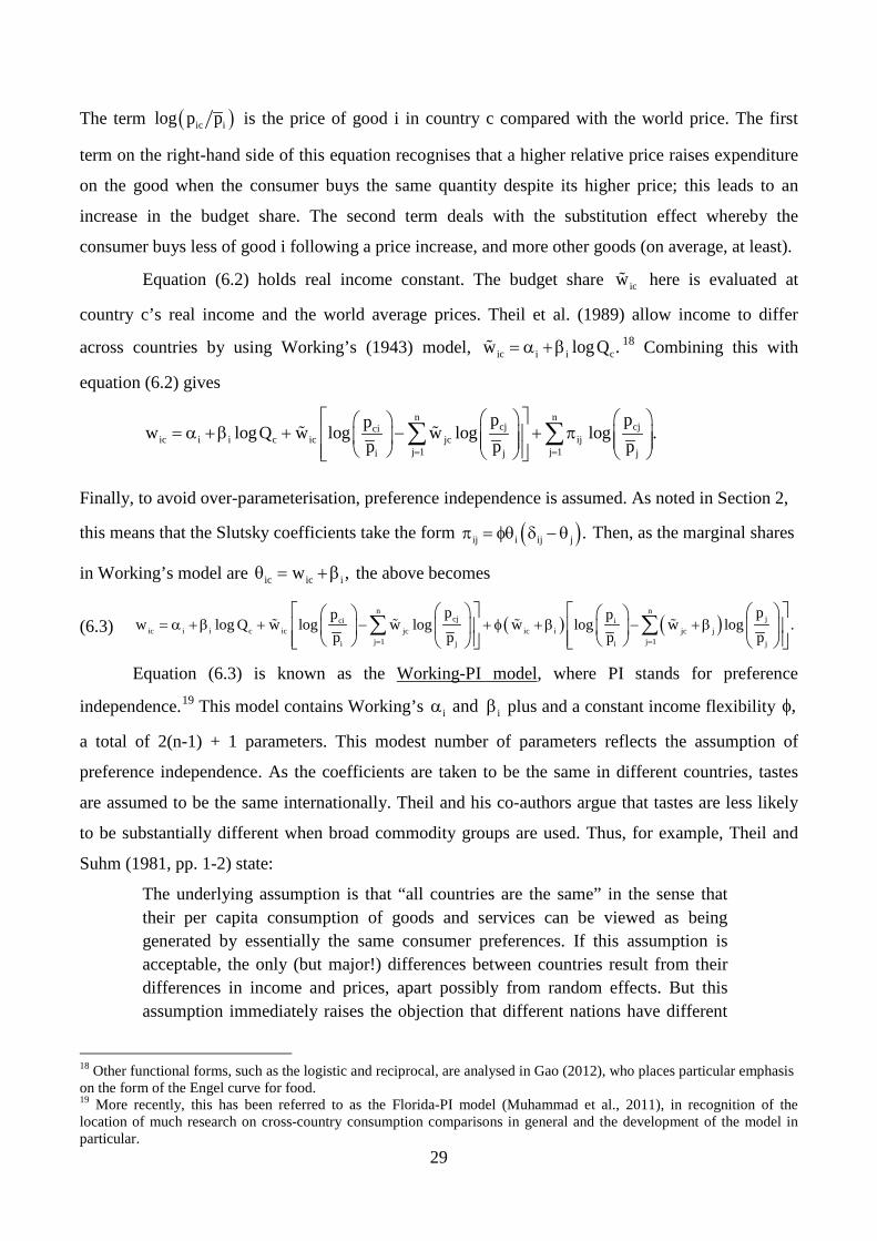
country c’s real income and the world average prices. Theil et al. (1989) allow income to differ

across countries by using Working’s (1943) model, ic i i cw logQ .= α + β

18 Combining this with

equation (6.2) gives

n ncj cjci

ic i i c ic jc ijj 1 j 1i j j

p ppw logQ w log w log log .p p p= =

= α + β + − + p

∑ ∑

Finally, to avoid over-parameterisation, preference independence is assumed. As noted in Section 2,

this means that the Slutsky coefficients take the form ( )ij i ij j .p = φq δ − q Then, as the marginal shares

in Working’s model are ic ic iw ,q = + β the above becomes

(6.3) ( ) ( )n n

cj jci iic i i c ic jc ic i jc j

j 1 j 1i j i j

p pp pw log Q w log w log w log w log .

p p p p= =

= α + β + − + φ + β − + β

∑ ∑

Equation (6.3) is known as the Working-PI model, where PI stands for preference

independence.19 This model contains Working’s i i and α β plus and a constant income flexibility ,φ

a total of 2(n-1) + 1 parameters. This modest number of parameters reflects the assumption of

preference independence. As the coefficients are taken to be the same in different countries, tastes

are assumed to be the same internationally. Theil and his co-authors argue that tastes are less likely

to be substantially different when broad commodity groups are used. Thus, for example, Theil and

Suhm (1981, pp. 1-2) state:

The underlying assumption is that “all countries are the same” in the sense that their per capita consumption of goods and services can be viewed as being generated by essentially the same consumer preferences. If this assumption is acceptable, the only (but major!) differences between countries result from their differences in income and prices, apart possibly from random effects. But this assumption immediately raises the objection that different nations have different

18 Other functional forms, such as the logistic and reciprocal, are analysed in Gao (2012), who places particular emphasis on the form of the Engel curve for food. 19 More recently, this has been referred to as the Florida-PI model (Muhammad et al., 2011), in recognition of the location of much research on cross-country consumption comparisons in general and the development of the model in particular.

29

cultures. We should expect that Indians spend little on meat and, indeed, the data produced by Kravis et al. [1982] confirm that this is so. The appropriate answer is that a cross-country demand system should be constructed, not for a very large number of detailed consumption categories, but only for a modest number of much broader categories. Accordingly, meat is part of a “good” called Food …20

7. CONCLUDING COMMENTS

Most economists are now familiar with and Deaton and Muellbauer’s (1980a) Almost Ideal

Demand System. This is a system of n demand equations whose form is obtained from an algebraic

specification of the consumer’s cost function, which can be thought of as an approximation to the

unknown true form. Similarly, the translog system (Christensen et al., 1975) to an approximation to

the unknown true form. Similarly, the translog system (Christensen et al., 1975) comes from a

specification of the indirect utility function, while the linear expenditure system (Stone, 1954)

derives from a specific direct utility function. Less familiar is the approach of the Rotterdam model

(Barten, 1964, Theil, 1965). Here, the precise form of the function to be optimised (the cost or utility

function) is left unspecified, but the general constraints of the utility-maximisation problem of

homogeneity (the absence of money illusion) and symmetry of the substitution effects are

incorporated into the demand equations. Working with a straightforward transform of demand

equations expressed in terms of differences in the logarithms (weighting them by the corresponding

budget shares), these constraints take the convenient form of linear parametric restrictions. The

question of functional form is therefore left until the last step in the Rotterdam approach, rather than

the first as in other approaches. The Rotterdam demand equations are thus interpreted as

approximations to the true, unknown ones. These demand equations provide a simple way to test the

theory of consumer demand, as well as the separability of preferences. The transparency of the

approach, and its generality, has contributed to the prominence of the Rotterdam model over the past

half-century. Some of the major events in the development of the model and its descendants are

listed in Table 2.

The 1960s were a period of rapid developments in econometrics with many breakthroughs,

one of which was the Rotterdam demand model. Interestingly, this occurred in Rotterdam, not at

either of the two Cambridges, that, at the time, laid claims to global leadership in economic research.

20 The assumption that tastes are constant is a major element of Chicago economics as practiced by Becker, Freidman and Stigler (Freidman, 1962, Stigler and Becker, 1977). Interestingly, while at Chicago, Theil’s approach to this issue seemed to evolve as earlier he argued that it was perfectly acceptable for tastes to be different in different countries: When describing the results from two independent applications of the Rotterdam model to Dutch and British time-series data with n = 4 goods, Theil (1975/76, vol.1, p. 208) writes “[t]he income elasticities of food agree with each other and they are of the order of magnitude which one would expect them to be, but the elasticities of the three other commodity groups show larger differences. There is no reason to be apologetic about this result, since different nations may have different preferences.” S. Selvanathan (1991, 1993) provides evidence that points towards the similarity of tastes for broad aggregates.

30

Why/how did this occur in the second city of a small, non-English-speaking country still recovering

from the ravages of war? Whatever the reason for this seemingly unlikely event, Barten and Theil

had the prescience to come up with an elegantly simple model that has stood the test of time and

their Rotterdam model is now one of the workhorses of applied demand analysis.21

There is still some lingering resistance to the model due to doubts about its microeconomic

foundations and the unconventional nature of its derivation. In marking the model’s golden jubilee,

this paper has emphasised its strong link with preferences and utility maximisation, highlighted its

strengths and weaknesses and shown how it has opened up new opportunities for creative research in

the form of the differential approach and cross-country consumption economics. By devoting

considerable attention to the derivation and interpretation of the model, our objective has been to

enhance understanding and make the Rotterdam system more accessible to economists. The paper

also emphasised that like all model, the Rotterdam is not perfect and involves familiar trade-offs

between generality, tractability and ease of interpretation. In addition to consumer demand, the

model (or variants thereof) have been applied to a range of other areas, including labour economics,

international trade, marketing, the economics of advertising, forecasting, regional economics,

monetary economics and the analysis of market structure in industrial organisation.22 It seems likely

that the Rotterdam model will continue to play an influential role in the future.

21 In discussion with Clements, Paul Frijters has pointed out that as Rotterdam was a long-standing centre of international trade, English was widely spoken there in the 1960s and its scholars were well connected with the rest-of-the-world academic community. He argues that research networks at that time centred more around individuals rather than locations. This can be taken to say that the physical/cultural aspects of 1960s Rotterdam were not particularly different from those of other centres of economic research. Perhaps the creation of the Rotterdam model in the context of Rotterdam of the 1960s was not as unlikely as implied by the text. 22 A selection of studies in these areas is as follows: In labour economics, Barnett (1979a, 1981) and Kiefer (1977); international trade, Berner (1977), Marquez (1994), Seale et al. (1992) and Theil and Clements (1978); marketing, Clements and E. A. Selvanathan (1988) and Vilcassim (1989); advertising, Duffy (1987) and E. A. Selvanathan (1989, 1995a,b); forecasting, E. A. Selvanathan (1995c); regional economics, S. Selvanathan (1991); monetary economics, Clements and Nguyen (1980), Fayyad (1986) and Offenbacher (1980); and industrial organisation, Capps et al. (2003). There have also been a numerous applications of the Rotterdam system to the demand for agricultural commodities.

31

References

Barnett, W. A. (1979a). “The Joint Allocation of Goods and Leisure Expenditure.” Econometrica 47: 539-63.

Barnett, W. A. (1979b). “Theoretical Foundations for the Rotterdam Model.” Review of Economic Studies 45: 109-130.

Barnett, W. A. (1981). Consumer Demand and Labour Supply: Goods, Monetary Assets and Time. Amsterdam: North-Holland Publishing Company.

Barnett, W. A. (1984). “On the Flexibility of the Rotterdam Model: A First Empirical Look.” European Economic Review 24: 285-89.

Barnett, W. A. (2003), “A Conversation with Henri (Hans) Theil: His Experiences in the Netherlands during the Second World War.” Journal of Agricultural and Applied Economics 35 Supplement: 57.

Barnett, W. A., and A. Serletis (2008). “Consumer Preferences and Demand Systems.” Journal of Econometrics 147: 210-24.

Barnett, W. A., and A. Serletis (2009). “The Differential Approach to Demand Analysis and the Rotterdam Model.” In D. J. Slottje (ed) Quantifying Consumer Preferences. Bingley, UK: Emerald Group Publishing. Pp.61 – 81.

Barten, A. P. (1964). “Consumer Demand Functions Under Conditions of Almost Additive Preferences.” Econometrica 32: 1-38.

Barten, A. P. (1967). “Evidence on the Slutsky Conditions for Consumer Demand.” Review of Economics and Statistics 49: 77-84.

Barten, A. P. (1968). “Estimating Demand Equations.” Econometrica 36: 213-51. Barten, A. P. (1977). “The Systems of Consumer Demand Functions Approach: A Review.”

Econometrica 45: 23-51. Barten, A. P. (1989). “Toward a Levels Version of the Rotterdam and Related Demand Systems.” In

B. Cornet and H. Tulkens (eds) Contributions to Operations Research and Economics: The Twentieth Anniversary of CORE. Cambridge, Mass. : MIT Press. Pp. 441-65.

Barten, A. P. (1993). “Consumer Allocation Models: Choice of Functional Form.” Empirical Economics 18:129-58.

Barten A. P., and L. J. Bettendorf (1989). “Price Formation of Fish: An Application of an Inverse Demand System.” European Economic Review 33: 1509-25.

Barten A. P., and E. Geyskens (1975). “The Negativity Condition in Consumer Demand.” European Economic Review 6: 227-60.

Berner, R. (1977). “Estimating Consumer Import Demand Equations.” International Finance Discussion Paper No. 105, Board of Governors of the Federal Reserve System, Washington, DC.

Bewley, R. A. (1986). Allocation Models: Specification, Estimation and Applications. Cambridge Mass: Ballinger Publishing Co.

Bewley, R. A. (2000). “Mr Henri Theil: An Interview with the International Journal of Forecasting.” International Journal of Forecasting 16: 1–16.

Blaug, M. , ed., (1999). Who’s Who in Economics. Third Edition. Cheltenham, UK and Northampton, MA, USA: Edward Elgar.

32

Blundell, R. (1988). “Consumer Behaviour: Theory and Empirical Evidence: A Survey.” Economic Journal 98: 16-65.

Brown, A., and A. Deaton, (1972). “Surveys in Applied Economics: Models of Consumer Behaviour.” Economic Journal 82: 1145-236.

Byron, R. P. (1984). “On the Flexibility of the Rotterdam Model.” European Economic Review 24: 273-84.

Capps, O., Jr., J. Church, H. A. Love (2003). “Specification Issues and Confidence Intervals in Unilateral Price Effects Analysis.” Journal of Econometrics 113: 3-31.

Chen, D. L. (1999). World Consumption Economics. Singapore: World Scientific Publishing. Christensen, L. R., D. W. Jorgenson and L. J. Lau (1975). “Transcendental Logarithmic Utility

Functions.” American Economic Review 65: 367-83. Clements, K. W., and P. Nguyen (1980). “Money Demand, Consumer Demand and Relative Prices in

Australia.” Economic Record 56: 338-46. Clements, K. W., and H. Theil (1979). “A Cross-Country Analysis of Consumption Patterns.” Report

7924 of the Center for Mathematical Studies in Business and Economics, The University of Chicago. Subsequently published in H. Theil Studies in Global Econometrics. Dordrecht: Kluwer Academic Publishers, 1996, pp. 95-108.

Clements, K. W., and E. A. Selvanathan (1988). “The Rotterdam Demand Model and its Application in Marketing.” Marketing Science 7: 60-75.

Clements, K. W., and S. Selvanathan (1994). “Understanding Consumption Patterns.” Empirical Economics 19: 69-110.

Deaton, A. S. (1974). “The Analysis of Consumer Demand in the United Kingdom, 1900-1970.” Econometrica 42: 341-67.

Deaton, A. S. (1986). “Demand Analysis.” In Z. Griliches and M. D. Intriligator (eds) Handbook of Econometrics. Volume III. Amsterdam: North-Holland Publishing Company. Pp. 1768-839.

Deaton, A. S., and J. Muellbauer (1980a). “An Almost Ideal Demand System.” American Economic Review 70: 312-26.

Deaton, A. S. and J. Muellbauer (1980b). Economics and Consumer Behaviour. Cambridge: Cambridge University Press.

Deaton, A. S., and C. Paxson (1998). “Economies of Scale, Household Size, and the Demand for Food.” Journal of Political Economy 106: 897-930.

DeJanvry, A., J. Bieri and A. Nunez (1972). “Estimation of Demand Parameters under Consumer Budgeting: An Application to Argentina.” American Journal of Agricultural Economics 54: 422-30.

Divisia, F. (1925). “L’indice Monetaire et la theorie de la monnaie.” Revue d’Economie Politique 39: 980-1008.

Duffy, M. H. (1987). “Advertising and the Inter-Product Distribution of Demand: A Rotterdam Model Approach.” European Economic Review 31: 1051-70.

Fayyad, S. K. (1986). “A Microeconomic System-Wide Approach to the Estimation of the Demand for Money.” Federal Reserve Bank of St Louis Review August-September: 22-33.

Friedman, M. (1962). Price Theory: A Provisional Text. Chicago: Aldine. Frisch, R. (1932). New Methods of Measuring Marginal Utility. Tubingen: J. C. B. Mohr. Frisch, R. (1959). “A Complete Scheme for Computing All Direct and Cross Demand Elasticities in

a Model with Many Sectors.” Econometrica 27: 177-96.

33

Gao, G. (2012). “World Food Demand.” American Journal of Agricultural Economics 94: 25-51. Geary, R. C. (1949-50). “A Note on a Constant Utility Index of the Cost of Living.” Review of

Economic Studies 18: 65-66. Goldberger, A. S. (1987). Functional Form and Utility: A Review of Consumer Demand Theory.

Boulder and London: Westview Press. Goldberger, A. S. and T. Gamaletsos (1970). “A Cross-Country Comparison of Consumer

Expenditure Patterns.” European Economic Review l: 357-400. Gorman, W. M. (1959). “Separability Utility and Aggregation.” Econometrica 27: 469-81. Gorman, W. M. (1968). “Conditions for Additive Separability.” Econometrica 36: 605-609. Horowitz, I. (1978). “Review of Heni Theil, Theory and Measurement of Consumer Demand.”

Interfaces 8: 109-11. Houthakker, H. S. (1957). “An International Comparison of Household Expenditure Patterns,

Commemorating the Centenary of Engel's Law.” Econometrica 25: 532-51. Houthakker, H. S. (1960). “Additive Preferences.” Econometrica 28: 244-57. Houthakker, H. S. (1965). “New Evidence on Demand Elasticities.” Econometrica 33: 277-88. Hymans, S. H., and H. T. Shapiro. 1976. “The Allocation of Household Income to Food

Consumption.” Journal of Econometrics 4: 167-88. Keifer, N. M. (1977). “A Bayesian Analysis of Commodity Demand and Labour Supply.”

International Economic Review 18: 209-18. Keller, W. J. (1984). “Some Simple but Flexible Differential Consumer Demand Systems.”

Economics Letters 16: 77-82. Keller, W. J. and J. van Driel (1985). “Differential Consumer Demand Systems.” European

Economic Review 27: 375-90. Klein, L. R. and H. Rubin (1948). “A Constant Utility Index of the Cost of Living.” Review of

Economic Studies 15: 84-87. Koerts, J. (1992). “Professor Theil’s Contributions to Economics.” In B. Raj and J. Koerts (eds)

Henri Theil’s Contributions to Economics and Econometrics. Dordrecht, Boston, London: Kluwer Academic Publishers. Volume 1, pp. 17-24.

Kravis, I. B., A. W. Heston and R. Summers (1982). World Product and Income: International Comparisons of Real Gross Product. Baltimore Md: The John Hopkins University Press.

Laitinen, K. (1978). “Why is Demand Homogeneity So Often Rejected?” Economics Letters 1: 187-9.

Leser, C. E. V. (1963). “Forms of Engel Functions.” Econometrica 31: 694-703. Lluch, C. and A. A. Powell (1975). “International Comparisons of Expenditure Patterns.” European

Economic Review 6: 375-303. Lluch, C., A. A. Powell and R. A. Williams (1977). Patterns in Household Demand and Saving.

Oxford: Oxford University Press. Marquez, J. (1994). “The Econometrics of Elasticities or the Elasticity of Econometrics: An

Empirical Analysis of the Behavior of US Imports.” Review of Economics and Statistics 76: 471-81.

Meade, B., A. Regmi, J. L. Seale, Jr., and A. Muhammad (2014). “New International Evidence on Food Consumption Patterns: A Focus on Cross-Price Effects Based on 2005 International Comparisons.” Technical Bulletin 1937. Economic Research Service, United States Department of Agriculture.

34

McFadden, D. (1964) “Existence Conditions for Theil-Type Preferences.” Unpublished paper, Department of Economics, University of California, Berkeley.

Meisner, J. F. (1979). “The Sad Fate of the Asymptotic Slutsky Symmetry Test for Large Systems.” Economics Letters 2: 231-33.

Mountain, D. C. (1988). “The Rotterdam Model: An Approximation in Variable Space.” Econometrica 56: 477-84.

Muellbauer, J. (1978). “Review of Theory and Measurement of Consumer Demand by Henri Theil.” Economic Journal 88: 161-63.

Muhammad, A., J. L. Seale, Jr., B. Meade, A. Regmi (2011). “International Evidence on Food Consumption Patterns: An Update Using 2005 International Comparison Program Data.” Technical Bulletin 1929. Economic Research Service, United States Department of Agriculture. Revised 2013.

Neves, P. D. (1994). “A Class of Differential Demand Systems.” Economics Letters 44: 83–86. Offenbacher, E. K. (1980). “The Basic Functions of Money: An Application of the Input

Independence Transformation. “ Economics Letters 5: 353-57. Parks, R. W. (1969). “Systems of Demand Equations: An Empirical Comparison of Alternative

Functional Forms.” Econometrica 37: 629-50. Parks, R. W., and A. P. Barten (1973). “A Cross-Country Comparison of the Effects of Prices,

Income and Population Composition on Consumption Patterns.” Economic Journal 83: 834-52.

Phlips, L. (1974). Applied Consumption Analysis. Amsterdam: North-Holland Publishing Company. Second edition 1983.

Pollak, R. A., and T. J. Wales (1987). “Pooling International Consumption Data.” Review of Economics and Statistics 69: 90-99.

Pollak, R. A., and T. J. Wales (1992). Demand System Specification and Estimation. New York and Oxford: Oxford University Press.Powell, A. A. (1974). Empirical Analytics of Demand Systems. Lexington Mass: DC Heath and Company.

Powell, A. A. (1974). Empirical Analytics of Demand Systems. Lexington Mass: DC Heath and Company.

Raj, B. (1992). “Henri Theil’s Biography and his Contributions to Economics and Econometrics: An Overview.” In B. Raj and J. Koerts (eds) Henri Theil’s Contributions to Economics and Econometrics. Dordrecht, Boston, London: Kluwer Academic Publishers. Volume 1, pp. 3-16.

Regmi, A., and J. L. Seale, Jr. (2010). “Cross-Price Elasticities of Demand Across 114 Countries.” Technical Bulletin No. 1925, Economic Research Service, United States Department of Agriculture.

Rimmer, M. T., and A. A. Powell (1992). “Demand Patterns Across the Development Spectrum: Estimates for the AIDADS System.” Preliminary Working Paper No. OP–75, Centre of Policy Studies and Impact Project, Monash University.

Seale, J. L., Jr, and C. B. Moss, eds, (2003). “Henri (Hans) Theil Memorial.” Journal of Agricultural and Applied Economics 35 Supplement.

Seale, J. L., Jr., and A. Regmi (2006). “Modelling International Consumption Patterns.” Review of. Income and Wealth 52: 603–24.

35

Seale, J. L., Jr., and A. Regmi (2009). “International Consumption Patterns: Evidence from the 1996 International Comparison Programme.” In S. Ghatak and P. Levine (eds), Development Macroeconomics: Essays in Memory of Anita Ghatak. Routledge, Taylor and Francis Group: London and New York. Pp. 252–99.

Seale, J. L., Jr., A. Regmi and A., J. Bernstein (2003). “International Evidence on Food Consumption Patterns.” Technical Bulletin 1904. Economic Research Service, United States Department of Agriculture, Washington, D.C.

Seale, J. L., Jr., and A. A. Solano (2012). “The Changing Demand for Energy in Rich and Poor Countries over 25 Years.” Energy Economics 34: 1834–44.

Seale, J. L., Jr., A. L. Sparks and B. M. Buxton (1992). “A Rotterdam Application to International Trade in Fresh Apples: A Differential Approach.” Journal of Agricultural and Resource Economics 17: 138-49.

Seale, J. L., Jr., W. E. Walker and I-M. Kim (1991). “The Demand for Energy: Cross-Country Evidence Using the Florida Model.” Energy Economics 13: 33-40.

Selvanathan, E. A. (1985). “An Even Simpler Differential Demand System.” Economics Letters 19: 343–47.

Selvanathan, E. A. (1989). “Advertising and Consumer Demand: A Differential Approach.” Economics Letters 31: 215-19.

Selvanathan, E. A. (1991). “Further Results on Aggregation of Differential Demand Equations.” Review of Economic Studies 58: 799-805.

Selvanathan, E. A. (1995a). “Advertising and Consumption: A Theoretical Analysis.” Chapter 7 in E. A. Selvanathan and K. W. Clements (eds) Recent Developments in Applied Demand Analysis: Alcohol, Advertising and Global Consumption. Berlin/Heidelberg: Springer-Verlag. Pp. 259-95.

Selvanathan, E. A. (1995b). “The Effects of Advertising on Alcohol Consumption: An Empirical Analysis.” Chapter 8 in E. A. Selvanathan and K. W. Clements (eds) Recent Developments in Applied Demand Analysis: Alcohol, Advertising and Global Consumption. Berlin/Heidelberg: Springer-Verlag. Pp. 297-340.

Selvanathan, E. A. (1995c). “The Rotterdam Model in Forecasting: An Application to the Alcohol Market.” Chapter 9 in E. A. Selvanathan and K. W. Clements (eds) Recent Developments in Applied Demand Analysis: Alcohol, Advertising and Global Consumption. Berlin/Heidelberg: Springer-Verlag. Pp. 341-58.

Selvanathan, S. (1991). “Regional Consumption Patterns in Australia: A System- Wide Analysis.” Economic Record 67: 338-45.

Selvanathan, S. (1993). A System-Wide Analysis of International Consumption Patterns. Boston, Dordrecht and London: Kluwer Academic Publishers.

Selvanathan, S., and E. A. Selvanathan (1994). Regional Consumption Patterns: A System-Wide Approach. London: Avebury Publishers.

Selvanathan, S. and E. A Selvanathan (2003). International Consumption Patterns: OECD versus LDC. Singapore: World Scientific.

Stigler, G. J., and G. S. Becker (1977). “De Gustibus Non Est Disputandum.” American Economic Review 67: 79-90.

Stone, R. (1954). “Linear Expenditure Systems and Demand Analysis: An Application to the Pattern of British Demand.” Economic Journal 64: 511-27.

36

Theil, H. (1965). “The Information Approach to Demand Analysis.” Econometrica 33: 67-87. Theil, H. (1967). Economics and Information Theory. New York: Elsevier/North-Holland, Inc. and

Amsterdam: North-Holland Publishing Company. Theil, H. (1971). Principles of Econometrics. New York: John Wiley and Sons. Theil, H. (1975/76). Theory and Measurement of Consumer Demand. Two Volumes. Amsterdam:

North-Holland Publishing Company. Theil, H. (1980). The System-Wide Approach to Microeconomics. Chicago: The University of Chicago Press.

Theil, H. (1987). “Evidence from International Consumption Comparisons.” Chapter 2 in H. Theil and K. W. Clements, Applied Demand Analysis: Results from System-Wide Approaches. Cambridge, Mass. : Ballinger. Pp. 37-100.

Theil, H. (1996). Studies in Global Econometrics. Dordrecht, Holland: Kluwer Academic Publishers. Theil, H. and R. Brooks (1970/71). “How does the Marginal Utility of Income Change when Real

Income Changes?” European Economic Review 2: 218-40. Theil, H., C-F. Chung and J. L. Seale, Jr (1989). International Evidence on Consumption Patterns.

Greenwich, Connecticut: JAI Press, Inc. Theil, H., and K. W. Clements (1978). “A Simple Method of Estimating Price Elasticities in

International Trade” (with H. Theil). Economics Letters 1: 133-37. Theil, H., and K. W. Clements (1987). Applied Demand Analysis: Results from System-Wide

Approaches. Cambridge Mass: Ballinger Publishing Co. Theil, H., and F. E. Suhm (1981). International Consumption Comparisons: A System-Wide

Approach. Amsterdam: North- Holland Publishing Company. Timmer, C. P., and H. Alderman (1979). “Estimating Consumption Parameters for Food Policy

Analysis.” American Journal of Agricultural Economics 61: 982-87. Vilcassim, N. J. (1989). “Extending the Rotterdam Model to Test Hierarchical Market Structures.”

Marketing Science 8: 181-90. Working, H. (1943). “Statistical Laws of Family Expenditure.” Journal of the American Statistical

Association 38: 43-56.

37

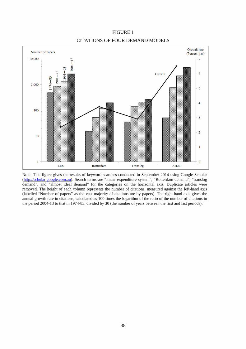
FIGURE 1

CITATIONS OF FOUR DEMAND MODELS

Note: This figure gives the results of keyword searches conducted in September 2014 using Google Scholar (http://scholar.google.com.au). Search terms are “linear expenditure system”, “Rotterdam demand”, “translog demand”, and “almost ideal demand” for the categories on the horizontal axis. Duplicate articles were removed. The height of each column represents the number of citations, measured against the left-hand axis (labelled “Number of papers” as the vast majority of citations are by papers). The right-hand axis gives the annual growth rate in citations, calculated as 100 times the logarithm of the ratio of the number of citations in the period 2004-13 to that in 1974-83, divided by 30 (the number of years between the first and last periods).

38

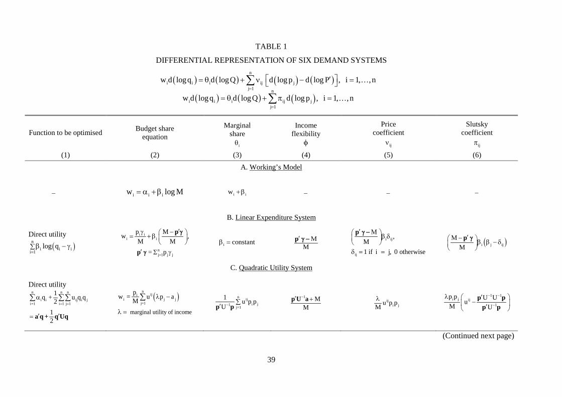
TABLE 1

DIFFERENTIAL REPRESENTATION OF SIX DEMAND SYSTEMS

( ) ( ) ( ) ( )

( ) ( ) ( )

n

i i i ij jj 1 n

i i i ij jj 1

w d logq d logQ d log p d log P , i 1, , n

w d logq d logQ d log p , i 1, , n =

=

′= q + ν − =

= q + p =

∑∑

Function to be optimised Budget share equation

Marginal share

iq

Income flexibility

φ

Price coefficient

ijν

Slutsky coefficient

ijp

(1) (2) (3) (4) (5) (6)

A. Working’s Model

− i i iw log M= α + β i iw + β

−

− −

B. Linear Expenditure System

Direct utility

( )n

i i ii 1

log q=∑ β − g

i ii i

nj 1 j j

p Mw ,M M

= p=

′g − = + β

′ Σ g

p

p

g

g i constantβ =

M

p′ Mg −

i ij

ij

,M1 if i j, 0 othe rwise=

′ M β δ δ =

p g − ( )i j ij

M

′M − β β − δ

p g

C. Quadratic Utility System

Direct utility n n n

i i ij i ji=1 i 1 j 1

1q + u q q212

= =α

′ ′=

∑ ∑∑

a q + q Uq

( )n

ijii j j

j=1

marginal utility of income

pw = u p aM λ −

λ =

∑ n ij

i j1j=1

1 u p pU− ∑′p p

1 MM

−′ +p U a iji ju p p

Mλ

1 1i j ij

1

p p U UuM U

− −

−

λ ′ − ′

p pp p

(Continued next page)

39

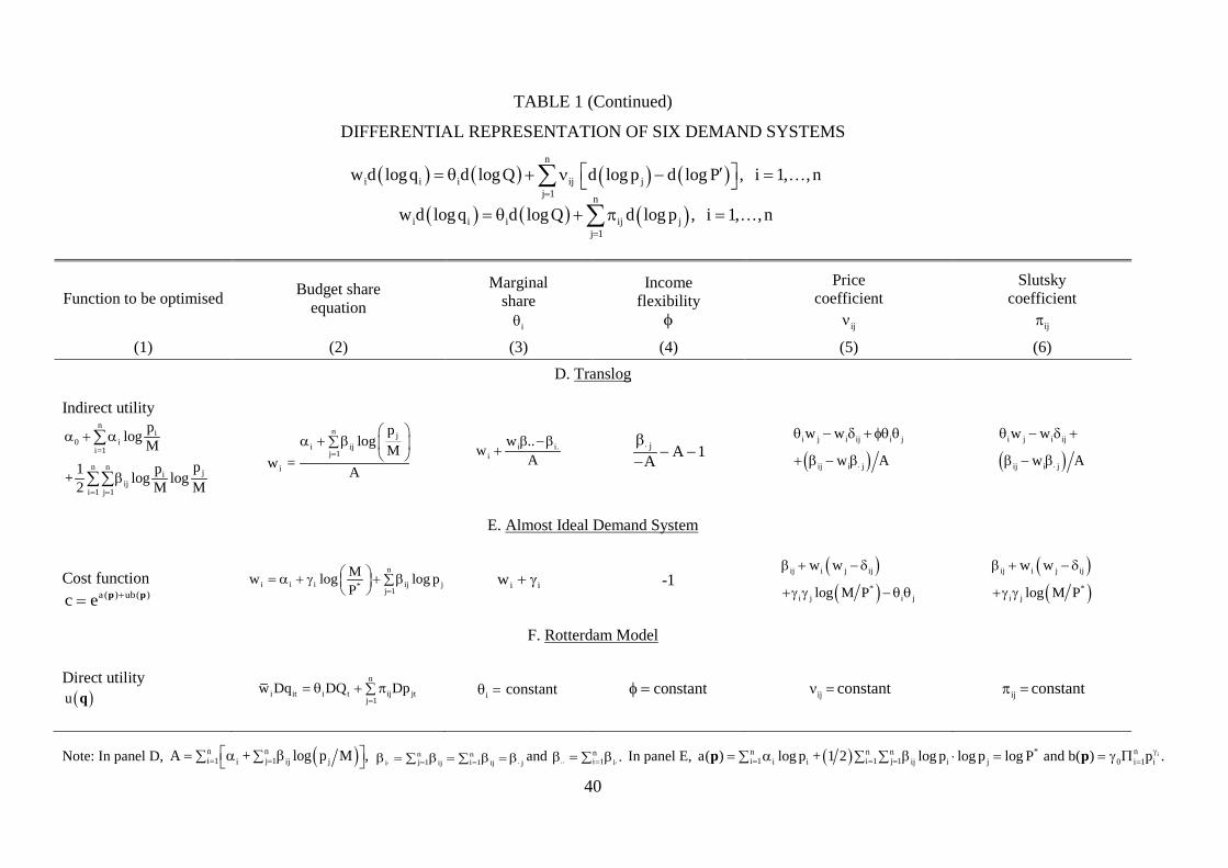
TABLE 1 (Continued)

DIFFERENTIAL REPRESENTATION OF SIX DEMAND SYSTEMS

( ) ( ) ( ) ( )

( ) ( ) ( )

n

i i i ij jj 1 n

i i i ij jj 1

w d logq d logQ d log p d log P , i 1, , n

w d logq d logQ d log p , i 1, , n =

=

′= q + ν − =

= q + p =

∑∑

Function to be optimised Budget share equation

Marginal share

iq

Income flexibility

φ

Price coefficient

ijν

Slutsky coefficient

ijp

(1) (2) (3) (4) (5) (6)

D. Translog

Indirect utility n

i0 i

i=1

n nji

iji 1 j 1

plog Mpp1+ log log2 M M= =

α + α

β

∑

∑∑

n ji ij

j 1

i

plog M

w =A

=

α + β∑

i i.

iw ..

wA

β − β+

j A 1A⋅β

− −−

( )i j i ij i j

ij i j

w w

w A⋅

q − δ + φq q

+ β − β ( )

i j i ij

ij i j

w w

w A⋅

q − δ +

β − β

E. Almost Ideal Demand System

Cost function

a( ) ub( )c e += p p

n

i i i ij j*j 1

Mw log log pP =

= α + g + β∑

i iw + g -1 ( )

( )ij i j ij

*i j i j

w w

log M P

β + − δ

+g g − q q

( )( )

ij i j ij

*i j

w w

log M P

β + − δ

+g g

F. Rotterdam Model

Direct utility ( )u q

n

i it i t ij jtj 1

w Dq DQ Dp=

= q + p∑ iq = constant constantφ = ijν = constant ijp = constant

Note: In panel D, ( )n ni 1 j 1i ij jA + log p M ,= = = α β∑ ∑ n n

j 1 i 1i ij ij j= =⋅ ⋅β = β = β = β∑ ∑ and ni 1 i .=⋅⋅ ⋅β = β∑ In panel E, ( ) i* nn n n

i 1 i 1 j 1i i ij i j 0 i 1 ia( ) log p + 1 2 log p log p log P and b( ) p .g= = = == α β ⋅ = = g Π∑ ∑ ∑p p

40

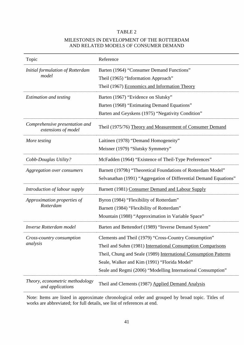
TABLE 2

MILESTONES IN DEVELOPMENT OF THE ROTTERDAM AND RELATED MODELS OF CONSUMER DEMAND

Topic Reference

Initial formulation of Rotterdam model

Barten (1964) “Consumer Demand Functions”

Theil (1965) “Information Approach”

Theil (1967) Economics and Information Theory

Estimation and testing Barten (1967) “Evidence on Slutsky”

Barten (1968) “Estimating Demand Equations”

Barten and Geyskens (1975) “Negativity Condition”

Comprehensive presentation and extensions of model Theil (1975/76) Theory and Measurement of Consumer Demand

More testing Laitinen (1978) “Demand Homogeneity”

Meisner (1979) “Slutsky Symmetry”

Cobb-Douglas Utility? McFadden (1964) “Existence of Theil-Type Preferences”

Aggregation over consumers Barnett (1979b) “Theoretical Foundations of Rotterdam Model”

Selvanathan (1991) “Aggregation of Differential Demand Equations”

Introduction of labour supply Barnett (1981) Consumer Demand and Labour Supply

Approximation properties of Rotterdam

Byron (1984) “Flexibility of Rotterdam”

Barnett (1984) “Flexibility of Rotterdam”

Mountain (1988) “Approximation in Variable Space”

Inverse Rotterdam model Barten and Bettendorf (1989) “Inverse Demand System”

Cross-country consumption analysis

Clements and Theil (1979) “Cross-Country Consumption”

Theil and Suhm (1981) International Consumption Comparisons

Theil, Chung and Seale (1989) International Consumption Patterns

Seale, Walker and Kim (1991) “Florida Model”

Seale and Regmi (2006) “Modelling International Consumption”

Theory, econometric methodology and applications Theil and Clements (1987) Applied Demand Analysis

Note: Items are listed in approximate chronological order and grouped by broad topic. Titles of works are abbreviated; for full details, see list of references at end.

41

Appendix

DERIVATIONS

The Linear Expenditure System

The ith equation of LES is

(A1) n

i i i i i j jj=1

p q p γ β M p γ ,

= + −

∑

or, dividing by income M,

(A2) i i iw s β r,= +

where i i iw p q M= is the budget share of goods i, i i is p γ M= is cost of subsistence of that good

expressed as a fractions of income, and ( )nj=1 j jr M p γ M= − ∑ is the supernumerary ratio.

The logarithmic differential of (A1) is

( ) ( ) ( ) ( ) ( )n

i i ii i i j j

j=1i i i

s β βd log p +d log q d log p d log M s d log p .w w w

= + − ∑

Multiplying both sides by iw and collecting terms, we have

( ) ( ) ( ) ( )n

i i i ij i i i j jj=1

w d log q β d log M δ s w β s d log p , = + − − ∑

where ijδ is the Kronecker delta. From (A2), i i is - w -β r, = so the term in square brackets above

is ( )i ij j-β rδ s .+ Using the Divisia decomposition of the charge in money income into real income

and price components, ( ) ( ) ( )d log M d log Q +d log P ,= where ( ) ( )ni=1 i id log P w d log p ,= ∑ the

above then becomes

( ) ( ) ( ) ( ) ( )

( ) ( ) ( )

n n

i i i j j i ij j jj=1 j=1

n

i i j ij jj=1

w d log q β d log Q + w d log p β rδ s d log p

β d log Q rβ β δ d log p ,

= − +

= + −

∑ ∑

∑

where the second step follows from (A2). Thus, LES can be expressed in term of the differential

demand equation as ( ) ( ) ( )ni i i i=1 ij jw d log q θ d log Q + π d log p ,= ∑ with marginal share i i ,q = β a

constant, and Slutsky coefficients ( )i j i j ijπ rβ β δ , variable.= − This verifies equation (5.4) of the

text.

The utility function underlying LES is

42

(A3) ( ) ( )n

1 n i i ii 1

u q , ,q log q ,=

= β − g∑

with ( )i i i i iu u q q≡ ∂ ∂ = β − g and ( ) ( )2 22ii i i i iu u q q .≡ ∂ ∂ = −β − g Dividing both sides of (A1)

by ip gives ( )( )ni i i i j=1 j jq γ β p M - p γ ,= + Σ which, when substituted into (A3), gives the indirect

utility function:

( )n n

iI 1 n i j j

ii 1 j 1

n n n n

i i i i i j ji 1 i 1 i 1 j 1

βu M,p , , p log M p γp

logβ log p log M p γ .

= =

= = = =

= β −

= β − β + β −

∑ ∑

∑ ∑ ∑ ∑

Thus, the marginal utility of income is ( )nI j 1 j ju M 1 M p ,=λ ≡ ∂ ∂ = − Σ g with

( )2nj 1 j jM 1 M p ,=∂λ ∂ = − − Σ g so that

( ) ( ) ( )1

2 n nnj j j jj j j 1 j 1j 1

log 1 M M r .log M 1 M - p , M - pM - p

−

= ==

∂ λ − −= ⋅ = = −

∂ g gg ∑ ∑∑

This shows that the income flexibility, ( ) 1log log M ,−φ = ∂ λ ∂ in LES equals the negative of the

supernumerary ratio.

For a utility maximum, each marginal utility is proportional to the corresponding price,

with the marginal utility of income the proportionality factor, i iu p ,= λ or

( ) ( )ni i j 1 j j i i ip u M - p q .== λ = Σ g β − g Thus, the ( )thi, i price coefficient associated with LES takes

the form

( )( )

( )( )

( )( )2n n

j 1 j j i j 1 j j i i ii i iiii in

j 1 j j i i i i i

M - p M - p qp p 1 1u ,M M - p q q M

= =

=

Σ g β Σ g β − gν = λ = − = φβ

Σ g − g − g β

where iiiiu 1 u .= As (A3) is additive, all second-order cross derivatives vanish, so that

ij 0, i j.ν = ≠ This confirms equation (5.5) of the text.

Quadratic Utility

The quadratic utility function is ( )1 nu q , ,q 1 2 ,′ ′= ⋅a q + q Uq and the corresponding

demand system is

(A4) 1

1 11

M= +−

− −−

′+−

′p U aq U a U p

p U p

Substituting, the indirect utility function is

43

1 1 11 1 1 1 1 1

1 1 1

1 1 11 1 1 1

1 1 1

11

M 1 M M+ + +2

M 1 M M= + + +2

M= +

p U a p U a p U aa U a a U p + U a U p U U a U pp U p p U p p U p

p U a p U a p U aa U a a U p + a U p U a pp U p p U p p U p

p U aa U ap

− − −− − − − − −

− − −

− − −− − − −

− − −

−−

′′ ′ ′ + + +′ ′− − − ′ ′ ′ ′ ′ ′ + + +′ ′ ′ ′− − − ′ ′ ′

′+′−′

( )

( )

211 11 1 1 1

1 1 1 1

211

1

M1 M M2

M1 1 .2 2

p U ap U a p U aa U p + a U a a U p p U aU p p U p p U p p U p

p U aa U a

p U p

−− −− − − −

− − − −

−−

−

′+′ ′+ + ′ ′ ′ ′− − +′ ′ ′

′+′= − +

′The marginal utility of income is and the income flexibility are

(A5) 1

1u M ,M

−

−

′∂ +λ = =

∂ ′p U a

p U p

1 1log M .log M M

− −′∂ λ + φ = = ∂ p U a

The demand equation for good i can also be expressed as (see text):

(A6) ( )n

iji j j

j 1q u p a .

== λ −∑

The total differential is ( )n iji j jj 1dq u dp p d== λ + λ∑ . Multiplying both sides by ip M , we have

(A7) ( ) ( )n n

ij iji ii i j j j

j 1 j 1

p pw d logq u p d log p u p d .M M= =

λ= + λ∑ ∑

From (A5), the differential of λ is

( )

( ) ( )

( ) ( )

1

1

n n n nij ij

j i i j j1 1i 1 j 1 i 1 j 1

n nij

i i j j1i 1 j 1

n n nij

i j j j j j1i 1 j 1 j 1

Md d

1 2dM u a dp u p p d log p

1 dM u a 2 p p d log p

1 dM u p p d log p p q d log p ,

p U ap U p

p U p p U p

p U p

p U p

−

−

− −= = = =

−= =

−= = =

′ +λ = ′

λ = + − ′ ′ = + − λ ′ = − λ − ′

∑∑ ∑∑

∑∑

∑∑ ∑

where the last step follows from (A6).

Using the above expression for dλ , the right-hand side of (A7) becomes

44

( )

( ) ( ) ( )

( ) ( )

n nij iji i

j j jj 1 j 1

n n n n nij ij iji i

j j j i j j j j j1j 1 j 1 i 1 j 1 j 1

n nij ijni j i jj 1 j 1 i jij iji

j j1 1j 1

p pu p d log p u p dM M

p p 1u p d log p u p dM u p p d log p p q d log pM M

u p p u p p p ppd log M u p d log p uM M

p U p

p U p p U p

= =

−= = = = =

= =− −

=

λ+ λ

λ = + − λ − ′

λ= + − λ

′ ′

∑ ∑

∑ ∑ ∑∑ ∑

∑ ∑∑ ( ) ( )

( ) ( ) ( ) ( )

( )

n n n

j j ji 1 j 1 j 1

n nij ijn n ni j i jj 1 j 1 i jij iji

j j j1 1j 1 i 1 j 1

n ij ij n iki jj 1 i j k jkji kk 1

1 1k

d log p w d log p

u p p u p p p ppd log M u p d log p u d log p d log PM M

u p p u p p p pu p pd logQ uM M

p U p p U p

p U p p U p

= = =

= =− −

= = =

= =− −

+

λ= + − λ + ′ ′

λ= + − λ

′ ′

∑∑ ∑

∑ ∑∑ ∑∑

∑ ∑ ( )n n

jj 1 1

d log p .= =

∑ ∑

The term in square brackets in the last line of the above can be simplified by noting that

equation (A5) implies

(A8) 1 ,M p U p−

λ φ=

′

so that term becomes ij ij kjn nik ikn n

i j k j i j k jkji k i kk 1 k 11 1 1

k 1 k 1

u p p p p u p p u p pu p p u p puM M M

= =− − −

= =

λ λ− λ = − φ ′ ′ ′

∑ ∑∑ ∑p U p p U p p U p

Equation (A7) can be formulated in absolute (or undeflated) prices as

( ) ( ) ( )n nnij ij jkikni jj 1 i j j ki k k 1k 1

i i j1 1 1j 1

u p p u p p u p pu p pw d logq d logQ d log p .Mp U p p U p p U p

= ==− − −=

∑ ∑∑∑

λ = + − φ ⋅ ′ ′ ′

This is the differential demand equation in absolute prices in the text.

To derive the relative price version, note that from equation (A8) ij

i j iji j1

u p pu p p ,M −

λ φ= ⋅

′p U p

or, summing over we have j 1, , n,=

n ijijn

i ji j j 11

j 1

u p pu p p.M p U p

=−

=

λ= φ

′∑

∑

Using this, the substitution term in the last line of the equation above (A8) can be written as

( )

( ) ( )

( ) ( )

ij n ikn ni j k jkji kk 1

j1j 1 k 1

ij kjn ikn n ni j k ji kk 1

j j1 1j 1 j 1 k 1

ij kjn n ni j k j

j j1j 1 j 1 k 1

u p p p pu p p u d log pM M

u p p u p pu p pd log p d log pM

u p p u p pd log p d log p .M

=−

= =

=− −

= = =

−= = =

λ− λ ′

λ= − φ

′ ′

λ= − ′

∑∑ ∑

∑∑ ∑∑

∑ ∑∑

p U p

p U p p U p

p U p

45

Retracing our steps, equation (A7) becomes

( ) ( ) ( ) ( )n nij ij jkn n

i jj 1 i j j kk 1i i j j1 1

j 1 j 1

u p p u p p u p pw d logq d logQ d log p d log p .Mp U p p U p

= =− −

= =

λ= + − ′ ′

∑ ∑∑ ∑

This is the differential demand equation for good i expressed in terms of relative prices that

corresponds to quadratic utility.

The Translog

The translog system is equation (5.9):

( )n

j 1i ij ji

+ log p Mw = , i=1, ,n.A

=α β∑

Writing this as i iw = A A, the total differential is

( )n

i i i kk 1

1dw = dA w dAA =− ∑ ,

Using ( )nj 1i ij jdA d log p M ,== β∑ we have

( ) ( ) ( ) ( )

( ) ( ) ( ) ( )

( ) ( ) ( )

n n n n n

i ij j ij i kj j kjj 1 j 1 k 1 j 1 j 1

n n n n

ij i kj j ij i kjj 1 k 1 j 1 k 1

ni i

ij i j jj 1

1dw = d log p d log M w d log p d log MA

1 1 w d log p w d log MA Aw 1 d log M w d log pA A

= = = = =

= = = =

⋅⋅ ⋅⋅

=

β − β − β − β∑ ∑ ∑ ∑ ∑

= β − β − β − β∑ ∑ ∑ ∑

β − β = + β − β∑

where nj 1i. ij ,=β = β∑ n

k 1j kj=⋅β = β∑ and ni 1.. i .= ⋅β = β∑

Next, combine the above expression for idw with the differential of the budget share,

( ) ( ) ( )i i i i i idw w d logq w d log p w d log M ,= + − to give:

( ) ( ) ( ) ( )ni i

i i i i ij ij i j jj 1

w 1w d logq w d log M Aw w d log p ,A A⋅⋅ ⋅

⋅=

β − β = + + − δ + β − β∑

As ( ) ( ) ( )d log M d log P d logQ ,= + with ( ) ( )nj 1 j jd log P w d log p=∑= and

( ) ( )nj 1 j jd logQ w d logq ,=∑= the above equation becomes

(A9) ( ) ( ) ( )

( ) ( )

nn k 1ij i kji i i i j i ij j

j 1

n

i ij jj 1

ww d logq d logQ w w d log pA

d logQ d log p .

=

=

=

β − β∑= q + q − δ +∑

= q + p∑

Here, the marginal shares and the Slutsky coefficients take the form

nk 1ij i kji i

i i ij i j i ij

ww w , w w .A A=⋅⋅ ⋅

β − β∑β − βq = + p = q − δ +

To obtain the differential form of the translog in relative prices, add and subtract

( )nj 1i j jd log p=φq q∑ from the right-hand side of the first equation in (A9):

46

( ) ( ) ( ) ( ) ( )

( ) ( ) ( ) ( )

( ) ( ) ( ) ( ) ( )

( ) ( ) ( ) ( )

nn n

i i i ij j i j j i j jj 1 j 1j 1

n

i ij i j j ij 1

nn

i ij i j j ij i jj 1j 1

n

i ij i j jj 1

i

w d logq d logQ d log p d log p d log p

d logQ d log p d logP

d logQ d log p d logP

d logQ d log p d logP

d lo

= ==

=

==

=

= q + p + φq q − φq q

′= q + p + φq q − φq

′= q + p + φq q − p + φq q

′= q + p + φq q −

= q

∑ ∑ ∑

∑

∑ ∑

∑

( ) ( ) ( )n

ij jj 1

gQ d log p d log P .=

′+ ν − ∑

The third line of the above follows from equations (4.6) and (4.7) in the form

( )nj 1 ij i j i .= p + φq q = φq∑ The ( )thi, j price coefficient in the above takes the form

nk 1ij i kj

ij i j i ij i j

ww w .A

=β − β∑ν = q − δ + + φq q

The Almost Ideal Demand System (AIDS)

According to equation (5.11), the thi equation of AIDS is

n

i i i ij j*j 1

Mw log log p ,P =

= α + g + β∑

so that ( ) ( ) ( )* nj 1i i i ij jdw d logM d log P d log p .== g − g + β∑ Subtracting from both sides

( ) ( )i i iw d log p w d log M− gives the quantity component of the change in the share:

( ) ( ) ( ) ( ) ( ) ( )n*i i i i i ij i ij j

j 1w d logq w d log M d log P w d log p .

== g + − g + β − δ∑

Substituting ( ) ( ) ( ) ( ) ( )* n n ni 1 i 1 j 1i i ij i jd log P d log p + 1 2 d log p d log p= = == α β ⋅∑ ∑ ∑ , and

replacing ( )d log M by ( ) ( )d log P d log Q ,+ where ( ) nj 1 j jd log P w d log p=∑= , gives

( ) ( ) ( ) ( ) ( ) ( )

( ) ( ) ( ) ( )

n ni

i i i i ij ij i i i j i j kj jk k jj 1 k 1

n n

i i ij ij i i i j i j i kj k jj 1 k 1

w d logq w d logQ w (w )w d log p d log p .2

w d logQ w (w )w d log p d log p ,

= =

= =

g = g + + β − δ + + g − g α − β + β∑ ∑ = g + + β − δ + + g − g α − g β∑ ∑

since kj jk.β = β It follows from equation (5.11) that ( )*nj 1i ij j i ilog p w log M P ,=α + β = − g∑ so the

substitution term in the above becomes

( ) ( )

( ) }{ ( )

( ) ( )

n n

ij ij i i i j i j i kj k jj 1 k 1

n *ij ij i i i j i j j j

j 1

n *ij ij i i j i j j

j 1

w (w )w d log p d log p

w (w )w w log M P d log p

w w w log M P d log p .

= =

=

=

β − δ + + g − g α − g β∑ ∑

= β − δ + + g − g − g∑

= β − δ + + g g∑

Thus, the differential version of AIDS, in absolute prices, is

47

(A10) ( ) ( ) ( )

( ) ( )

n

i i i i ij ij i i j i j j*j 1

n

i ij jj 1

Mw d log q w d log Q w w w log d log pP

d log Q d log p ,

=

=

= g + + β − δ + + g g∑ = q + p∑

where ( )*ij ij ij i i j i jw w w log M Pp = β − δ + + g g are the implied Slutsky coefficients. The above is

equation (5.12) of the text.

As noted in the previous section, ( )nj 1 ij i j i .= p + φq q = φq∑ Thus, adding and then subtracting

( )nj 1i j jd log p=φq q∑ from the right-hand side of the first equation in (A10) gives the relative price

version of AIDS in differential form:

( ) ( ) ( )

( )( ) ( )

( ) ( ) ( )

i i i i

n

ij ij i i j i j i i j j j*j 1

n

i ij jj 1

w d logq w d log Q

Mw w w log w w d log p dlogPP

d log Q d log p d log P ,

=

=

= g +

′+ β − δ + + g g − + g + g −

′= q + ν −

∑

∑

where the ( )thi, j price coefficient is ( ) ( )*ij ij i j ij i j i jw w log M P .ν = β + − δ + g g − q q This is

equation (5.13) of the text.

48

Editor, UWA Economics Discussion Papers: Ernst Juerg Weber Business School – Economics University of Western Australia 35 Sterling Hwy Crawley WA 6009 Australia Email: ecoadmin@biz.uwa.edu.au The Economics Discussion Papers are available at: 1980 – 2002: http://ecompapers.biz.uwa.edu.au/paper/PDF%20of%20Discussion%20Papers/ Since 2001: http://ideas.repec.org/s/uwa/wpaper1.html Since 2004: http://www.business.uwa.edu.au/school/disciplines/economics

ECONOMICS DISCUSSION PAPERS 2012

DP NUMBER AUTHORS TITLE

12.01 Clements, K.W., Gao, G., and Simpson, T.

DISPARITIES IN INCOMES AND PRICES INTERNATIONALLY

12.02 Tyers, R. THE RISE AND ROBUSTNESS OF ECONOMIC FREEDOM IN CHINA

12.03 Golley, J. and Tyers, R. DEMOGRAPHIC DIVIDENDS, DEPENDENCIES AND ECONOMIC GROWTH IN CHINA AND INDIA

12.04 Tyers, R. LOOKING INWARD FOR GROWTH

12.05 Knight, K. and McLure, M. THE ELUSIVE ARTHUR PIGOU

12.06 McLure, M. ONE HUNDRED YEARS FROM TODAY: A. C. PIGOU’S WEALTH AND WELFARE

12.07 Khuu, A. and Weber, E.J. HOW AUSTRALIAN FARMERS DEAL WITH RISK

12.08 Chen, M. and Clements, K.W. PATTERNS IN WORLD METALS PRICES

12.09 Clements, K.W. UWA ECONOMICS HONOURS

12.10 Golley, J. and Tyers, R. CHINA’S GENDER IMBALANCE AND ITS ECONOMIC PERFORMANCE

12.11 Weber, E.J. AUSTRALIAN FISCAL POLICY IN THE AFTERMATH OF THE GLOBAL FINANCIAL CRISIS

12.12 Hartley, P.R. and Medlock III, K.B. CHANGES IN THE OPERATIONAL EFFICIENCY OF NATIONAL OIL COMPANIES

12.13 Li, L. HOW MUCH ARE RESOURCE PROJECTS WORTH? A CAPITAL MARKET PERSPECTIVE

12.14 Chen, A. and Groenewold, N. THE REGIONAL ECONOMIC EFFECTS OF A REDUCTION IN CARBON EMISSIONS AND AN EVALUATION OF OFFSETTING POLICIES IN CHINA

12.15 Collins, J., Baer, B. and Weber, E.J. SEXUAL SELECTION, CONSPICUOUS CONSUMPTION AND ECONOMIC GROWTH

49

ECONOMICS DISCUSSION PAPERS 2012

DP NUMBER AUTHORS TITLE

12.16 Wu, Y. TRENDS AND PROSPECTS IN CHINA’S R&D SECTOR

12.17 Cheong, T.S. and Wu, Y. INTRA-PROVINCIAL INEQUALITY IN CHINA: AN ANALYSIS OF COUNTY-LEVEL DATA

12.18 Cheong, T.S. THE PATTERNS OF REGIONAL INEQUALITY IN CHINA

12.19 Wu, Y. ELECTRICITY MARKET INTEGRATION: GLOBAL TRENDS AND IMPLICATIONS FOR THE EAS REGION

12.20 Knight, K. EXEGESIS OF DIGITAL TEXT FROM THE HISTORY OF ECONOMIC THOUGHT: A COMPARATIVE EXPLORATORY TEST

12.21 Chatterjee, I. COSTLY REPORTING, EX-POST MONITORING, AND COMMERCIAL PIRACY: A GAME THEORETIC ANALYSIS

12.22 Pen, S.E. QUALITY-CONSTANT ILLICIT DRUG PRICES

12.23 Cheong, T.S. and Wu, Y. REGIONAL DISPARITY, TRANSITIONAL DYNAMICS AND CONVERGENCE IN CHINA

12.24 Ezzati, P. FINANCIAL MARKETS INTEGRATION OF IRAN WITHIN THE MIDDLE EAST AND WITH THE REST OF THE WORLD

12.25 Kwan, F., Wu, Y. and Zhuo, S. RE-EXAMINATION OF THE SURPLUS AGRICULTURAL LABOUR IN CHINA

12.26 Wu, Y. R&D BEHAVIOUR IN CHINESE FIRMS

12.27 Tang, S.H.K. and Yung, L.C.W. MAIDS OR MENTORS? THE EFFECTS OF LIVE-IN FOREIGN DOMESTIC WORKERS ON SCHOOL CHILDREN’S EDUCATIONAL ACHIEVEMENT IN HONG KONG

12.28 Groenewold, N. AUSTRALIA AND THE GFC: SAVED BY ASTUTE FISCAL POLICY?

50

ECONOMICS DISCUSSION PAPERS 2013

DP NUMBER AUTHORS TITLE

13.01 Chen, M., Clements, K.W. and Gao, G.

THREE FACTS ABOUT WORLD METAL PRICES

13.02 Collins, J. and Richards, O. EVOLUTION, FERTILITY AND THE AGEING POPULATION

13.03 Clements, K., Genberg, H., Harberger, A., Lothian, J., Mundell, R., Sonnenschein, H. and Tolley, G.

LARRY SJAASTAD, 1934-2012

13.04 Robitaille, M.C. and Chatterjee, I. MOTHERS-IN-LAW AND SON PREFERENCE IN INDIA

13.05 Clements, K.W. and Izan, I.H.Y. REPORT ON THE 25TH PHD CONFERENCE IN ECONOMICS AND BUSINESS

13.06 Walker, A. and Tyers, R. QUANTIFYING AUSTRALIA’S “THREE SPEED” BOOM

13.07 Yu, F. and Wu, Y. PATENT EXAMINATION AND DISGUISED PROTECTION

13.08 Yu, F. and Wu, Y. PATENT CITATIONS AND KNOWLEDGE SPILLOVERS: AN ANALYSIS OF CHINESE PATENTS REGISTER IN THE US

13.09 Chatterjee, I. and Saha, B. BARGAINING DELEGATION IN MONOPOLY

13.10 Cheong, T.S. and Wu, Y. GLOBALIZATION AND REGIONAL INEQUALITY IN CHINA

13.11 Cheong, T.S. and Wu, Y. INEQUALITY AND CRIME RATES IN CHINA

13.12 Robertson, P.E. and Ye, L. ON THE EXISTENCE OF A MIDDLE INCOME TRAP

13.13 Robertson, P.E. THE GLOBAL IMPACT OF CHINA’S GROWTH

13.14 Hanaki, N., Jacquemet, N., Luchini, S., and Zylbersztejn, A.

BOUNDED RATIONALITY AND STRATEGIC UNCERTAINTY IN A SIMPLE DOMINANCE SOLVABLE GAME

13.15 Okatch, Z., Siddique, A. and Rammohan, A.

DETERMINANTS OF INCOME INEQUALITY IN BOTSWANA

13.16 Clements, K.W. and Gao, G. A MULTI-MARKET APPROACH TO MEASURING THE CYCLE

13.17 Chatterjee, I. and Ray, R. THE ROLE OF INSTITUTIONS IN THE INCIDENCE OF CRIME AND CORRUPTION

13.18 Fu, D. and Wu, Y. EXPORT SURVIVAL PATTERN AND DETERMINANTS OF CHINESE MANUFACTURING FIRMS

13.19 Shi, X., Wu, Y. and Zhao, D. KNOWLEDGE INTENSIVE BUSINESS SERVICES AND THEIR IMPACT ON INNOVATION IN CHINA

13.20 Tyers, R., Zhang, Y. and Cheong, T.S.

CHINA’S SAVING AND GLOBAL ECONOMIC PERFORMANCE

13.21 Collins, J., Baer, B. and Weber, E.J. POPULATION, TECHNOLOGICAL PROGRESS AND THE EVOLUTION OF INNOVATIVE POTENTIAL

13.22 Hartley, P.R. THE FUTURE OF LONG-TERM LNG CONTRACTS

13.23 Tyers, R. A SIMPLE MODEL TO STUDY GLOBAL MACROECONOMIC INTERDEPENDENCE

51

ECONOMICS DISCUSSION PAPERS 2013

DP NUMBER AUTHORS TITLE

13.24 McLure, M. REFLECTIONS ON THE QUANTITY THEORY: PIGOU IN 1917 AND PARETO IN 1920-21

13.25 Chen, A. and Groenewold, N. REGIONAL EFFECTS OF AN EMISSIONS-REDUCTION POLICY IN CHINA: THE IMPORTANCE OF THE GOVERNMENT FINANCING METHOD

13.26 Siddique, M.A.B. TRADE RELATIONS BETWEEN AUSTRALIA AND THAILAND: 1990 TO 2011

13.27 Li, B. and Zhang, J. GOVERNMENT DEBT IN AN INTERGENERATIONAL MODEL OF ECONOMIC GROWTH, ENDOGENOUS FERTILITY, AND ELASTIC LABOR WITH AN APPLICATION TO JAPAN

13.28 Robitaille, M. and Chatterjee, I. SEX-SELECTIVE ABORTIONS AND INFANT MORTALITY IN INDIA: THE ROLE OF PARENTS’ STATED SON PREFERENCE

13.29 Ezzati, P. ANALYSIS OF VOLATILITY SPILLOVER EFFECTS: TWO-STAGE PROCEDURE BASED ON A MODIFIED GARCH-M

13.30 Robertson, P. E. DOES A FREE MARKET ECONOMY MAKE AUSTRALIA MORE OR LESS SECURE IN A GLOBALISED WORLD?

13.31 Das, S., Ghate, C. and Robertson, P. E.

REMOTENESS AND UNBALANCED GROWTH: UNDERSTANDING DIVERGENCE ACROSS INDIAN DISTRICTS

13.32 Robertson, P.E. and Sin, A. MEASURING HARD POWER: CHINA’S ECONOMIC GROWTH AND MILITARY CAPACITY

13.33 Wu, Y. TRENDS AND PROSPECTS FOR THE RENEWABLE ENERGY SECTOR IN THE EAS REGION

13.34 Yang, S., Zhao, D., Wu, Y. and Fan, J.

REGIONAL VARIATION IN CARBON EMISSION AND ITS DRIVING FORCES IN CHINA: AN INDEX DECOMPOSITION ANALYSIS

52

ECONOMICS DISCUSSION PAPERS 2014

DP NUMBER AUTHORS TITLE

14.01 Boediono, Vice President of the Republic of Indonesia

THE CHALLENGES OF POLICY MAKING IN A YOUNG DEMOCRACY: THE CASE OF INDONESIA (52ND SHANN MEMORIAL LECTURE, 2013)

14.02 Metaxas, P.E. and Weber, E.J. AN AUSTRALIAN CONTRIBUTION TO INTERNATIONAL TRADE THEORY: THE DEPENDENT ECONOMY MODEL

14.03 Fan, J., Zhao, D., Wu, Y. and Wei, J. CARBON PRICING AND ELECTRICITY MARKET REFORMS IN CHINA

14.04 McLure, M. A.C. PIGOU’S MEMBERSHIP OF THE ‘CHAMBERLAIN-BRADBURY’ COMMITTEE. PART I: THE HISTORICAL CONTEXT

14.05 McLure, M. A.C. PIGOU’S MEMBERSHIP OF THE ‘CHAMBERLAIN-BRADBURY’ COMMITTEE. PART II: ‘TRANSITIONAL’ AND ‘ONGOING’ ISSUES

14.06 King, J.E. and McLure, M. HISTORY OF THE CONCEPT OF VALUE

14.07 Williams, A. A GLOBAL INDEX OF INFORMATION AND POLITICAL TRANSPARENCY

14.08 Knight, K. A.C. PIGOU’S THE THEORY OF UNEMPLOYMENT AND ITS CORRIGENDA: THE LETTERS OF MAURICE ALLEN, ARTHUR L. BOWLEY, RICHARD KAHN AND DENNIS ROBERTSON

14.09

Cheong, T.S. and Wu, Y. THE IMPACTS OF STRUCTURAL RANSFORMATION AND INDUSTRIAL UPGRADING ON REGIONAL INEQUALITY IN CHINA

14.10 Chowdhury, M.H., Dewan, M.N.A., Quaddus, M., Naude, M. and Siddique, A.

GENDER EQUALITY AND SUSTAINABLE DEVELOPMENT WITH A FOCUS ON THE COASTAL FISHING COMMUNITY OF BANGLADESH

14.11 Bon, J. UWA DISCUSSION PAPERS IN ECONOMICS: THE FIRST 750

14.12 Finlay, K. and Magnusson, L.M. BOOTSTRAP METHODS FOR INFERENCE WITH CLUSTER-SAMPLE IV MODELS

14.13 Chen, A. and Groenewold, N. THE EFFECTS OF MACROECONOMIC SHOCKS ON THE DISTRIBUTION OF PROVINCIAL OUTPUT IN CHINA: ESTIMATES FROM A RESTRICTED VAR MODEL

14.14 Hartley, P.R. and Medlock III, K.B. THE VALLEY OF DEATH FOR NEW ENERGY TECHNOLOGIES

14.15 Hartley, P.R., Medlock III, K.B., Temzelides, T. and Zhang, X.

LOCAL EMPLOYMENT IMPACT FROM COMPETING ENERGY SOURCES: SHALE GAS VERSUS WIND GENERATION IN TEXAS

14.16 Tyers, R. and Zhang, Y. SHORT RUN EFFECTS OF THE ECONOMIC REFORM AGENDA

14.17 Clements, K.W., Si, J. and Simpson, T. UNDERSTANDING NEW RESOURCE PROJECTS

14.18 Tyers, R. SERVICE OLIGOPOLIES AND AUSTRALIA’S ECONOMY-WIDE PERFORMANCE

53

ECONOMICS DISCUSSION PAPERS 2014

DP NUMBER AUTHORS TITLE

14.19 Tyers, R. and Zhang, Y. REAL EXCHANGE RATE DETERMINATION AND THE CHINA PUZZLE

14.20 Ingram, S.R. COMMODITY PRICE CHANGES ARE CONCENTRATED AT THE END OF THE CYCLE

14.21 Cheong, T.S. and Wu, Y. CHINA'S INDUSTRIAL OUTPUT: A COUNTY-LEVEL STUDY USING A NEW FRAMEWORK OF DISTRIBUTION DYNAMICS ANALYSIS

14.22 Siddique, M.A.B., Wibowo, H. and Wu, Y.

FISCAL DECENTRALISATION AND INEQUALITY IN INDONESIA: 1999-2008

14.23 Tyers, R. ASYMMETRY IN BOOM-BUST SHOCKS: AUSTRALIAN PERFORMANCE WITH OLIGOPOLY

14.24 Arora, V., Tyers, R. and Zhang, Y. RECONSTRUCTING THE SAVINGS GLUT: THE GLOBAL IMPLICATIONS OF ASIAN EXCESS SAVING

14.25 Tyers, R. INTERNATIONAL EFFECTS OF CHINA’S RISE AND TRANSITION: NEOCLASSICAL AND KEYNESIAN PERSPECTIVES

14.26 Milton, S. and Siddique, M.A.B. TRADE CREATION AND DIVERSION UNDER THE THAILAND-AUSTRALIA FREE TRADE AGREEMENT (TAFTA)

14.27 Clements, K.W. and Li, L. VALUING RESOURCE INVESTMENTS

14.28 Tyers, R. PESSIMISM SHOCKS IN A MODEL OF GLOBAL MACROECONOMIC INTERDEPENDENCE

14.29 Iqbal, K. and Siddique, M.A.B. THE IMPACT OF CLIMATE CHANGE ON AGRICULTURAL PRODUCTIVITY: EVIDENCE FROM PANEL DATA OF BANGLADESH

14.30 Ezzati, P. MONETARY POLICY RESPONSES TO FOREIGN FINANCIAL MARKET SHOCKS: APPLICATION OF A MODIFIED OPEN-ECONOMY TAYLOR RULE

14.31 Tang, S.H.K. and Leung, C.K.Y. THE DEEP HISTORICAL ROOTS OF MACROECONOMIC VOLATILITY

14.32 Arthmar, R. and McLure, M. PIGOU, DEL VECCHIO AND SRAFFA: THE 1955 INTERNATIONAL ‘ANTONIO FELTRINELLI’ PRIZE FOR THE ECONOMIC AND SOCIAL SCIENCES

14.33 McLure, M. A-HISTORIAL ECONOMIC DYNAMICS: A BOOK REVIEW

14.34 Clements, K.W. and Gao, G. THE ROTTERDAM DEMAND MODEL HALF A CENTURY ON

54