Embed Size (px)
Citation preview

ECONOMICS
PRICE RELATIONSHIPS IN VEGETABLE OIL AND
ENERGY MARKETS
by
Rini Yayuk Priyati Business School
University of Western Australia
and
Rod Tyers Business School
University of Western Australia, Research School of Economics, ANU
DISCUSSION PAPER 16.11

PRICE RELATIONSHIPS IN VEGETABLE OIL AND ENERGY MARKETS*
Rini Yayuk Priyati Business School, UWA
Rod Tyers
Business School University of Western Australia,
Research School of Economics, ANU
For presentation at the annual Australasian Development Economics Workshop Deakin University, 9-10 June 2016
DISCUSSION PAPER 16.11 Abstract
The markets for vegetable oils have expanded significantly in recent decades in association with the diversification in their use across final consumption as food, industrial inputs and fuels. International markets for such products remain critically important for several developing countries yet they have become more integrated globally and volatility has increased as financial determinants of demand have become more prominent. This paper reviews these developments in vegetable oil and energy markets and tests for changes in their level of integration over time. It further examines the dependence of prices in these markets on financial volatility and overall economic performance, offering scenarios for vegetable oil market behaviour in response to low energy prices, tighter monetary policy and strong demand in importing regions. The results are particularly strong in response to changes in interest rates, supporting the perspective that financial determinants of demand have strengthened.
Key words: Vegetable oils, Volatility, Market Integration, Financialization
* Thanks are due to Peter Robertson and the UWA Business School for research support and useful comments during work in progress seminars.

1
1. Introduction
Edible oil markets have grown substantially over the last two decades with a tripling of
production of the nine major vegetable oils: coconut, cottonseed, groundnut, olive, palm,
palm kernel, rapeseed, soybean, and sunflower oils. While all have expanded, the dominant
growth has been in palm oil production. As of 2013, palm oil accounted for 35 percent of
total vegetable oil production, followed by soybean oil (26 percent) and rapeseed oil (15
percent). It has been increasingly traded with the dominant exporters being Indonesia and
Malaysia and the dominant importers being India, the European Union and China. At the
same time the vegetable oil group has also been increasingly used as feedstock in energy
production. With these changes, and the increasing integration of markets for storable
commodities with those for other financial assets (Baffles and Haniotis 2016, Ohashi and
Okimoto 2016), price volatility has risen during the past decade.
This paper quantifies the trend toward the integration of vegetable oil markets, amongst
themselves and with other energy products, and examines the determinants of intertemporal
changes in of vegetable oil prices. Our research has two goals. First, we seek to explore the
level of integration within vegetable oil groups. In doing so, the bulk of the work follows the
research by In and Inder (1997), who group vegetable oils based by their end-uses in the food
industry and find co-integration only between sunflower, soybean and rapeseed oils.
Commodity markets have changed considerably since their work and, moreover, our analysis
differs from theirs in that vegetable oils are clustered based on end-uses that are not limited to
the food industry. The greater diversity of modern end uses is evident from data obtained
from USDA-FAS (2015b). Our results suggest that the substitutability among major
vegetable oils occurs within, rather than between, end-use clusters. Additionally, the pattern
of price volatility also follows end-use groups.

2
Second, we examine the relationships between vegetable oil, energy and financial markets
and overall economic performance. Sanders et al. (2014) observe the driving factors behind
the recent palm oil boom and the role of both food and fuel demands by analysing the long
and short run relationships between palm oil, soybean oil and crude petroleum prices. Their
results suggest that the recent palm oil boom is driven by food market demand rather than
energy markets. We find some role for energy market effects, operating through the demand
side, since palm oil is a consumption substitute for vegetable oils that can be used as fuels. A
stronger relationship occurs with interest rates, however, suggesting the integration of these
markets with those of financial assets. We adopt an elemental VAR approach to estimate
these relationships and to forecast the sensitivity of vegetable oil prices to growth in
consuming regions, the petroleum price and bond yields in integrated financial markets.
The paper is organised as follows. The section to follow offers some background on
vegetable oil markets and prices and it reviews recent published work on their behaviour. In
Section 3 we focus on changes in comparative volatility of vegetable oil and petroleum
markets. Section 4 then re-examines the integration of these markets in the light of recent
data on price movements. Links to financial markets and overall economic performance are
then examined in Section 5. Discussions of the implications of energy and financial market
shocks, and global growth in demand for vegetable oils, are then provided in Section 6.
Section 7 concludes.
2. Vegetable Oil Markets and their Price Behaviour
Growth paths for output of all the oils are shown in Figure 1. The dominant vegetable oil is
palm oil, which is mostly produced in Indonesia and Malaysia. Its recent growth has been an
important contributor to those countries’ overall economic performance. For Malaysia, palm
oil accounted for 4 percent of its total GDP in 2013, up from 3 percent in 2005 (DOSM,

3
2014). For Indonesia, the share of palm oil to total GDP is smaller than Malaysia at only 0.4
percent in 2005, but it increased to 0.8 percent in 2008 (BPS, 2006, BPS, 2009). However,
palm oil contributed 11 percent of Indonesia’s total merchandise exports in 2014, up from
only 2 percent in 2000 (WITS, 2015). While for Malaysia, it accounted for 2.6 percent in
2000 and 5.5 percent in 2014 of Malaysia’s total merchandise exports (WITS, 2015). This
recent growth in palm oil production has made Indonesia and Malaysia the two largest
exporters of vegetable oil.
Other large vegetable oil producers are China and the US (soybean oil), and the European
Union (rapeseed oil). Unlike Indonesia and Malaysia, however, their production is almost all
consumed domestically. On the demand side, India is the third largest consumer but almost
all of its consumption comes from imports. The global production, exports, and domestic
consumption of major vegetable oils is summarised in Table 1.
Several major vegetable oils are believed to be technically substitutable. This is reflected in
the similarities in their price patterns. Even though each vegetable oil has unique
characteristics, they are substitutes in the food sector as well as in industrial applications.
The choice of which oil is to be used is mostly based on the relative price among oils
(Griffith and Meilke, 1979, Owen et al., 1996). It can be seen from Figure 2 that the prices of
all oils seem to move similarly through time.

4
Figure 1. Major vegetable oil productions (million metric tonnes)
Source: USDA-FAS (2015b)
Unsurprisingly given the energy applications of some vegetable oils and the
“financialization” of storable commodities, petroleum prices have followed similar price
patterns, as depicted in Figure 2. The sharpest increase in commodity prices during recent
decades took place in 2008. During the first quarter of 2000 to the second quarter of 2008,
the average real price of vegetable oils (deflated by the U.S CPI) increased by more than 150
percent, while the petroleum price increased by approximately 250 percent. The relationships
between energy and food market prices have been a focus in several papers, including Zhang
et al. (2010), Ciaian (2011), Serra (2011), Nazlioglu and Soytas (2012), Reboredo (2012) and
Nazlioglu et al. (2013). Papers addressing closely related issues are also addressed by Yu et
al. (2006), Abdel and Arshad (2008), Peri and Baldi (2010) and Sanders et al. (2014).
0
10
20
30
40
50
60
70
1964
1965
1966
1967
1968
1969
1970
1971
1972
1973
1974
1975
1976
1977
1978
1979
1980
1981
1982
1983
1984
1985
1986
1987
1988
1989
1990
1991
1992
1993
1994
1995
1996
1997
1998
1999
2000
2001
2002
2003
2004
2005
2006
2007
2008
2009
2010
2011
2012
2013
Coconut
Cottonseed
Olive
Palm
Palm Kernel
Groundnut
Rapeseed
Soybean
Sunflower
5
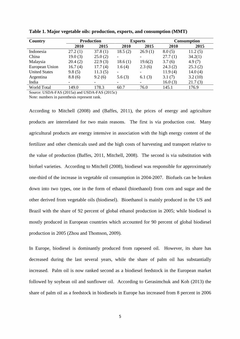
Table 1. Major vegetable oils: production, exports, and consumption (MMT)
Country Production Exports Consumption 2010 2015 2010 2015 2010 2015
Indonesia 27.2 (1) 37.8 (1) 18.5 (2) 26.9 (1) 8.0 (5) 11.2 (5) China 19.0 (3) 25.0 (2) - - 27.7 (1) 34.2(1) Malaysia 20.4 (2) 22.9 (3) 18.6 (1) 19.6(2) 3.7 (6) 4.9 (7) European Union 16.7 (4) 17.7 (4) 1.6 (4) 2.3 (6) 24.3 (2) 25.3 (2) United States 9.8 (5) 11.3 (5) - - 11.9 (4) 14.0 (4) Argentina 8.8 (6) 9.2 (6) 5.6 (3) 6.1 (3) 3.1 (7) 3.2 (10) India - - - - 16.0 (3) 21.7 (3) World Total 149.0 178.3 60.7 76.0 145.1 176.9 Source: USDA-FAS (2015a) and USDA-FAS (2015c) Note: numbers in parenthesis represent rank.
According to Mitchell (2008) and (Baffes, 2011), the prices of energy and agriculture
products are interrelated for two main reasons. The first is via production cost. Many
agricultural products are energy intensive in association with the high energy content of the
fertilizer and other chemicals used and the high costs of harvesting and transport relative to
the value of production (Baffes, 2011, Mitchell, 2008). The second is via substitution with
biofuel varieties. According to Mitchell (2008), biodiesel was responsible for approximately
one-third of the increase in vegetable oil consumption in 2004-2007. Biofuels can be broken
down into two types, one in the form of ethanol (bioethanol) from corn and sugar and the
other derived from vegetable oils (biodiesel). Bioethanol is mainly produced in the US and
Brazil with the share of 92 percent of global ethanol production in 2005; while biodiesel is
mostly produced in European countries which accounted for 90 percent of global biodiesel
production in 2005 (Zhou and Thomson, 2009).
In Europe, biodiesel is dominantly produced from rapeseed oil. However, its share has
decreased during the last several years, while the share of palm oil has substantially
increased. Palm oil is now ranked second as a biodiesel feedstock in the European market
followed by soybean oil and sunflower oil. According to Gerasimchuk and Koh (2013) the
share of palm oil as a feedstock in biodiesels in Europe has increased from 8 percent in 2006

6
to 20 percent in 2012, while the share of rapeseed oil as a biodiesel feedstock has decreased
from 66 percent to 57 percent.
Figure 2. Vegetable and petroleum nominal price indices (1980q1=100)
Data source: IMF (2015a), UNCTADSTAT (2015), and World-Bank (2015) . Indices are author’s calculation (1980q1=100).
Some studies of vegetable oil prices have focussed on the relationships amongst vegetable oil
prices (Owen et al., 1997, Amiruddin et al., 2005, In and Inder, 1997) while others have
emphasised the links between vegetable oil prices and the prices of other goods, mostly other
agricultural goods or energy prices (Yu et al., 2006, Campiche et al., 2007, Abdel and
Arshad, 2008, Harri et al., 2009, Peri and Baldi, 2010, Hassouneh et al., 2012, Sanders et al.,
2014). The latter studies depend on the assumption that energy and vegetable oil markets are
linked together due to the demand for vegetable oils as inputs to the biofuels sector, which
has strengthened with rises in crude petroleum prices. All these studies above employed co-
integration analysis.
For the price relationships within vegetable oils, the results of co-integration tests thus
obtained are mixed. Owen et al. (1997) find no co-integration among their samples. They
0
50
100
150
200
250
300
350
400
450
1980
Q1
1981
Q1
1982
Q1
1983
Q1
1984
Q1
1985
Q1
1986
Q1
1987
Q1
1988
Q1
1989
Q1
1990
Q1
1991
Q1
1992
Q1
1993
Q1
1994
Q1
1995
Q1
1996
Q1
1997
Q1
1998
Q1
1999
Q1
2000
Q1
2001
Q1
2002
Q1
2003
Q1
2004
Q1
2005
Q1
2006
Q1
2007
Q1
2008
Q1
2009
Q1
2010
Q1
2011
Q1
2012
Q1
2013
Q1
2014
Q1
CoconutCottonseedGroundnutPalmPalm kernelRapeseedSoybeanSunflowerPetroleum

7
analyse the price interrelationships in the vegetable and tropical oils markets using price time
series for the five major oils (coconut, palm, palm kernel, soybean and sunflower oil)
between 1971 and 1993. They use a first-differenced VAR since they observe no co-
integrating relationship amongst oil prices. Using variance decomposition analysis they
found that, first, palm kernel and coconut oil (lauric oils) prices interacted strongly, but
neither had a strong relationship with other oil prices. Second, the palm oil price was found
to have a lower level of interaction with other oil prices; and third, greater interaction could
be found between soybean and sunflower oil prices than between the other oil prices (Owen
et al., 1997). These results are consistent with a global market dominated by soybean oil.
They are of little relevance today since the structure of oils markets has changed radically.
At around the same time In and Inder (1997) investigated the long run relationship between
world vegetable oil prices using multivariate co-integration analysis. Using a sample of eight
oils, they first constructed three groups based on differences in use: (a) general oils (soybean,
cottonseed, rapeseed, sunflower, and palm oils), (b) groundnut oil, (c) coconut and palm
kernel oils. Their data was monthly from October 1976 to March 1990. They expected that
there would be five co-integrating vectors, four for group (a) and one for group (c). Yet they
found only two co-integration relationships; between sunflower oil and soybean oil and
between sunflower oil and rapeseed oil. While their method is of interest, their data also
referenced a very different global market from that we observe today.
More recently, Amiruddin et al. (2005) examined the competition for Malaysian palm oil
from other vegetable oils. Using monthly data from January 1990 to June 2004, they
observed the prices of refined, bleached, and deodorised (RBD) palm oil, soybean oil,
sunflower oil, and rapeseed oil. They found one co-integration vector among those oils.
Using a VECM (vector error correction model), they concluded that soybean oil is the price

8
leader. Their approach is also of interest, though their results still reflect an outdated
characterisation of global vegetable oil markets.
A second recent literature on vegetable oil markets explores the relationships between the
pricing of vegetable oils and other goods, mostly petroleum. Yu et al. (2006) focus on the
long run relationship between the prices of oils from soybean, palm, rapeseed, and sunflower,
and petroleum. Among these five oil prices, they find that there is one co-integrating vector.
However, they find that the petroleum price does not influence the prices of vegetable oils.
They also anticipate a stronger relationship as the petroleum price and the use of vegetable
oils as biofuel continue to increase. Adding one more variable, palm oil, Abdel and Arshad
(2008) also examine the relationships between vegetable oils and petroleum. Using a
bivariate relationship between petroleum and each of these vegetable oils, they find that each
pair is co-integrated. Moreover, their causality tests suggest that there are unidirectional
causalities from the petroleum price to each of the vegetable oil prices.
Covering more agricultural commodities, rather than just vegetable oils, Campiche et al.
(2007) examine the correspondence between the prices of petroleum and corn, wheat, oats,
soybeans, soybean meal, and soybean oil. Using weekly price data, they break down the
analysis into two time periods, 2003-2005 and 2006-2007. Their Johansen co-integration
tests show that there is no co-integration between all price series during 2003-2005.
However, corn and soybean prices are co-integrated with the petroleum price during 2006-
2007 (Campiche et al., 2007). Harri et al. (2009) then add foreign exchange rates and cotton
prices to the analysis. Using recursive date tests from January 2000 to September 2008, they
observe co-integration relationships between petroleum and cotton prices, starting from June
2004, and between petroleum and corn, between soybean and soybean oil, and between
petroleum, corn, and exchange rates, all starting from April 2006.
9
Peri and Baldi (2010) observe the long run connection between prices of diesel oil and three
vegetable oils (rapeseed, sunflower, and soybean oils) during 2005 and 2007. Their findings
are that: first, the co-integration relationship only exists between rapeseed oil and diesel oil,
while, the combination of soybean and diesel oils and sunflower and diesel oils are not co-
integrated, second, the long run equilibrium of the rapeseed oil price is influenced by the
price of diesel oil, but not the other way. This is due to the high quota given to rapeseed oil
as a feedstock in Europe’s biodiesel industry. Third, this relationship between diesel and
rapeseed oil prices has growth stronger over time. A more recent study of these price
linkages, in this case between biodiesel, sunflower oil and crude oil prices, finds that there is
co-integration (Hassouneh et al. 2012). Here again, this is seen to represent the cost of
feedstock, while the positive relationship between biodiesel and crude oil represents the fact
that they used in blended form.
Most recently, Sanders et al. (2014) examine the food versus non-food demand drivers
behind the palm oil boom by assessing the long run and short run relationships between palm
oil, soybean oil, and petroleum prices. Their tests suggest that a co-integration relationship
exists among the three oils. In the short run, the price of petroleum does not affect the price
of palm oil while the price of soybean oil appears to affect the palm oil price. In the long run,
there exists co-integration among these oil prices. Ordinary least squares (OLS) estimates
suggest a negative relationship between palm oil and petroleum prices and a positive
relationship between palm oil and soybean oil prices. These results imply that, in the long
run, the boom in palm oil industry is driven by food and industrial demands rather than
changes in energy markets.

10
3. Trends in levels and volatility of vegetable oil and petroleum prices
Since the beginning of the 2000’s, the prices of vegetable oils have increased, following a
relatively stable trend from the late of 1970’s, as indicated in Figure 2. The average price
indices of vegetable oils increased by nearly 35 percent in 2003-2007 compared to 1998-2002
and increased by almost 74 percent in 2008-2014 compared to in 2003-2007 (Table 2). This
price surge was accompanied wilder movements that led also to increases in measures of
volatility, as shown in Figure 3.1
Table 2. Average price indices and volatilities
Period Average prices indices* Average volatility Vegetable oils
Petroleum Vegetable oils and petroleum
Vegetable oils
Petroleum Vegetable oils and petroleum
Whole period 108.15 113.53 108.75 0.20 0.18 0.19 1983-1987 85.68 66.19 83.52 0.26 0.12 0.24 1988-1992 79.08 52.87 76.17 0.17 0.19 0.17 1993-1997 96.15 50.35 91.06 0.13 0.12 0.13 1998-2002 77.36 61.03 75.55 0.15 0.22 0.16 2003-2007 112.02 143.57 115.53 0.18 0.19 0.18 2008-2014 185.83 274.52 195.69 0.23 0.17 0.22 Data source: IMF (2015a), UNCTADSTAT (2015), and World-Bank (2015) . * Index is author calculation (1980q1=100).
Volatility levels were higher during 1980’s, relatively low during1990’s and have increased
again since late 1990’s. Some vegetable oils, like palm oil, palm kernel oil and coconut oil
were more volatile than other vegetable oils during 1980’s, due to the financial and currency
volatility in that period. The real exchange rates of the two major importers of vegetable oils,
the German Deutsche Mark and (to a lesser extent) the Indian Rupee, appreciated against US
dollar from the first quarter of 1985 to the first quarter of 1988, following the Plaza Accord
(Figure 4). These exchange rate fluctuations matter because those three vegetable oils were
1 These volatilities are calculated using the coefficient of variation of the level of real prices using 12-quarter moving average. The formulation is:
( ) ( ) ( )1/2
2
1standard deviation / mean / /
n
ii
CV P P n P=
= = − ∑
where, CV is the coefficient variation, P is price level and P is the 12-quarter price average.

11
more traded than other vegetable oils and the US dollar was the currency in which their trade
transactions were denominated.
Figure 3. Nominal price volatilities
Data source: Volatilities are author’s calculations based on IMF (2015a), UNCTADSTAT (2015), and World-Bank (2015) .
Figure 5 shows the average exports to total production ratios of vegetable oils during 1980 to
2014. We can see that palm oil had been the most tradable vegetable oil in the 1980’s with a
ratio of more than 70 percent, followed by palm kernel oil and coconut oil at 60 percent and
50 percent level of ratios, respectively. These high trade ratios suggest global market
integration, leading to different price behaviours.
4. Clustering of Vegetable oils and petroleum markets and their integration
Some vegetable oils have more specific end uses than others, yet all vegetable oils are
technically substitutable. Owen et al. (1996) argued that the choice between oils was
dominated by their relative prices. The majority of the more recent literature sees pricing
behaviour as tied to end uses, however. We therefore take end use specificity seriously and
0
0.1
0.2
0.3
0.4
0.5
0.6
0.7
1983
Q1
1984
Q1
1985
Q1
1986
Q1
1987
Q1
1988
Q1
1989
Q1
1990
Q1
1991
Q1
1992
Q1
1993
Q1
1994
Q1
1995
Q1
1996
Q1
1997
Q1
1998
Q1
1999
Q1
2000
Q1
2001
Q1
2002
Q1
2003
Q1
2004
Q1
2005
Q1
2006
Q1
2007
Q1
2008
Q1
2009
Q1
2010
Q1
2011
Q1
2012
Q1
2013
Q1
2014
Q1
CoconutCottonseedGroundnutPalmPalm kernelRapeseedSoybeanSunflowerPetroleum

12
classify vegetable oils into three clusters. Cluster 1 includes coconut and palm kernel oils,
known also as lauric oils, which are heavily used by manufacturing industries. Cluster 2 is a
group of vegetable oils heavily used for food but that is also increasingly in demand for
industrial purposes. This group includes palm, soybean, and rapeseed oils. Cluster 3
includes sunflower, cottonseed, olive, and groundnut oils, a group of vegetable oils whose
dominant application is in food preparation.
Figure 4. Real exchange rate indices of German Deutsche Mark and Indian Rupee against US Dollar*
Source: author’s calculation (1980Q1=1) based on FRED (2015) Real exchange rates are calculated using:
, ,
*, )( /
i t i t t i tRER e p p= × , where ,i te represents the nominal
exchange rate between the US$ and the home country currency, tp represents the price level in home
country and *,i tp represents the price level in the US.
The proportion of the production of each oil product that is used for industrial purposes is
indicated in Figure 6, which shows quite significant changes over time for those oils with
faster overall consumption growth. Industrial applications of the lauric oils and those in
Cluster 2 can be anything from pharmaceuticals, cosmetics, biodiesel, and machine
lubricants. The trend for biodiesel use is strongest in European market, which accounted for
90 percent of global biodiesel production in 2005 (Zhou and Thomson, 2009). In Europe,
0
0.2
0.4
0.6
0.8
1
1.2
1980
Q1
1980
Q4
1981
Q3
1982
Q2
1983
Q1
1983
Q4
1984
Q3
1985
Q2
1986
Q1
1986
Q4
1987
Q3
1988
Q2
1989
Q1
1989
Q4
1990
Q3
1991
Q2
1992
Q1
1992
Q4
1993
Q3
1994
Q2
1995
Q1
1995
Q4
1996
Q3
1997
Q2
1998
Q1
1998
Q4
German DM
Indian Rupee

13
while rapeseed oil is the most important feedstock for biodiesel, increasing quantities of palm
oil, soybean oil and sunflower oil are now in use, as indicated in Table 3. Because sunflower
is also an important feedstock to biodiesel, we include it in Cluster 2, along with palm oil,
rapeseed oil, and soybean oil.
Figure 5. Average exports to production ratios
Source: author’s calculation based on USDA-FAS (2015b)
Based on their price volatilities, we can see that some oils have similar patterns to petroleum
and others do not (Figure 7). If the vegetable oils are grouped based on their price patterns
we find that the price grouping conforms approximately to the end use grouping. The
clusters we adopt are therefore as follows. Cluster 1 includes coconut and palm kernel oils,
which have almost identical price patterns and no clear relationship with the petroleum price.
Cluster 2 has palm, rapeseed, soybean and sunflower oils, which have related end use mixes
and price movements linked to the petroleum price. Cluster 3 includes cottonseed and
groundnut oils, which have random price patterns and do not have clear relationships with
petroleum. Note here that we exclude olive oil from the analysis due to its very specific end
use and its different price movement compared to all vegetable oils.
0
0.1
0.2
0.3
0.4
0.5
0.6
0.7
0.8
0.9
1980-1987 1988-1992 1993-1997 1998-2002 2003-2007 2008-2014
Coconut
Cottonseed
Groundnut
Palm
Palm Kernel
Rapeseed
Soybean
Sunflower

14
Table 3. Vegetable oils as biodiesel feedstock in European Union (1,000 MT)
Vegetable oil 2009 2010 2011 2012 2013 2014e 2015f Rapeseed oil 6300 6700 6600 6150 5770 6170 5970 Palm oil 550 690 700 1050 1640 1620 1630 Soybean oil 1000 1085 1000 685 850 850 855 Sunflower oil 170 140 240 260 265 280 285 Other (pine oil) 0 0 80 140 154 180 185
Adapted from USDA-FAS (2015), e=estimate, f=forecast.
The high volumes of production of the Cluster 2 oils (Figure 6) indicate that these are the
most commonly available as well as the most widely traded internationally and readily stored.
Their price behaviours can therefore be expected to be influenced more than the others by
global economic performance and financial market indicators.
4.1. Data
The data on vegetable oil prices are obtained from IMF Primary Commodity Prices (IMF,
2015a), UNCTAD’s Free Market Commodity Prices (UNCTADSTAT, 2015) and World
Bank Commodity Market Statistics, also known as the Pink Data (World-Bank, 2015). All
vegetable oil prices are expressed in US$ per metric tonne (MT). The original data are
available monthly but are averaged up to quarterly for conformity with the data on economic
determinants considered later.
Table 4. Summary statistics for vegetable oil and petroleum prices (in logs)
Oil Mean Standard deviation
Skewness Kurtosis Observations
Coconut 6.46 0.43 0.31 3.00 140 Palm kernel 6.43 0.42 0.28 3.04 140 Palm 6.09 0.43 0.30 2.45 140 Rapeseed 6.41 0.40 0.55 2.51 140 Soybean 6.33 0.35 0.73 3.04 140 Sunflower 6.53 0.40 0.89 3.23 140 Cottonseed 6.56 0.32 0.83 3.52 140 Groundnut 6.87 0.39 0.48 2.98 140
Data source: IMF (2015a), UNCTADSTAT (2015), and World-Bank (2015) . Note: all series are presented in natural logarithm (ln).

15
Figure 6. Global consumption of major vegetable oils: food versus industrial uses (thousand metric tonnes)
Source: (USDA-FAS, 2015b)
0500
10001500200025003000350040004500
1980
1982
1984
1986
1988
1990
1992
1994
1996
1998
2000
2002
2004
2006
2008
2010
2012
2014
Coconut Food
Industrial
0
5000
10000
15000
20000
25000
30000
1980
1982
1984
1986
1988
1990
1992
1994
1996
1998
2000
2002
2004
2006
2008
2010
2012
2014
Rapeseed
Food
Industrial
0
1000
2000
3000
4000
5000
6000
1980
1982
1984
1986
1988
1990
1992
1994
1996
1998
2000
2002
2004
2006
2008
2010
2012
2014
Cottonseed Food
Industrial
010002000300040005000600070008000
1980
1982
1984
1986
1988
1990
1992
1994
1996
1998
2000
2002
2004
2006
2008
2010
2012
2014
Palm kernel
Food
Industrial
0
10000
20000
30000
40000
50000
1980
1982
1984
1986
1988
1990
1992
1994
1996
1998
2000
2002
2004
2006
2008
2010
2012
2014
Soybean
Food
Industrial
0
1000
2000
3000
4000
5000
6000
1980
1982
1984
1986
1988
1990
1992
1994
1996
1998
2000
2002
2004
2006
2008
2010
2012
2014
Groundnut Food
Industrial
0
10000
20000
30000
40000
50000
60000
70000
1980
1982
1984
1986
1988
1990
1992
1994
1996
1998
2000
2002
2004
2006
2008
2010
2012
2014
Palm
Food
Industrial
02000400060008000
10000120001400016000
1980
1982
1984
1986
1988
1990
1992
1994
1996
1998
2000
2002
2004
2006
2008
2010
2012
2014
Sunflower
Food
Industrial
0
500
1000
1500
2000
2500
3000
3500
1980
1982
1984
1986
1988
1990
1992
1994
1996
1998
2000
2002
2004
2006
2008
2010
2012
2014
Olive Food
Industrial

16
Figure 7. Average volatilities on vegetable oil prices
(a) All vegetable oils (b) Cluster 1
(c) Cluster 2 (d) Cluster 3
0
0.05
0.1
0.15
0.2
0.25
0.3
0.35
0.4
1983-1987 1988-1992 1993-1997 1998-2002 2003-2007 2008-2014
CoconutCottonseedGroundnutPalmPalm kernelRapeseedSoybeanSunflowerPetroleum
0
0.05
0.1
0.15
0.2
0.25
0.3
0.35
0.4
1983-1987 1988-1992 1993-1997 1998-2002 2003-2007 2008-2014
Coconut
Palm kernel
Petroleum
0
0.05
0.1
0.15
0.2
0.25
0.3
0.35
1983-1987 1988-1992 1993-1997 1998-2002 2003-2007 2008-2014
Palm
Rapeseed
Soybean
Sunflower
Petroleum
0
0.05
0.1
0.15
0.2
0.25
0.3
1983-1987 1988-1992 1993-1997 1998-2002 2003-2007 2008-2014
Cottonseed
Groundnut
Petroleum

17
4.2. Co- integration
To determine the stationarity of the series, we conduct three unit root tests on each series,
namely the Augmented Dickey-Fuller (ADF), the Phillips-Perron (PP), and Kwiatkowski-
Phillips-Schmidt-Shin (KPSS) tests. Significant statistics for ADF and PP imply that we can
reject the null hypothesis of unit roots. Table 5 shows the results of these tests. Most of the
series appear to be I(1) at the 1% significant level. However, we find that some series are
I(0) for either ADF or PP, like coconut oil, groundnut oil, and palm kernel oil. To resolve
these conflicts we also conduct the KPSS test. This differs from the ADF and PP tests,
allowing us to reject the null hypothesis of stationarity when the KPSS statistic shows
significance. For all series, based on KPSS, the null hypothesis of stationarity is rejected at
the 1% significant level. Thus, we conclude that all price series are I(1). This is also
confirmed by a further series of unit root tests conducted on first differences.
Table 5. Unit root tests for real price of oils
Series ADF PP KPSS Levels lnCoconut(2) -4.03** -3.25 0.37** lnPalmkernel(2) -3.78* -3.43 0.36** lnPalm(2) -2.96 -2.99 0.44** lnRapeseed(2) -3.27 -2.82 0.51** lnSoybean(2) -3.00 -2.72 0.54** lnSunflower(2) -3.50* -3.31 0.52** lnCottonseed (3) -3.58* -3.58* 0.39** lnGroundnut(2) -4.41** -3.24 0.32** First differences lnCoconut(1) -6.38** -7.33** 0.03 lnPalmkernel(1) -7.08** -7.94** 0.03 lnPalm(2) -6.53** -8.22** 0.03 lnRapeseed(1) -7.06** -9.04** 0.05 lnSoybean(1) -7.96** -9.26** 0.04 lnSunflower(1) -8.17** -9.16** 0.02 lnCottonseed (2) -7.11** -7.75** 0.02 lnGroundnut(1) -6.59** -7.43** 0.03
Note:Numbers of lags selected are in the parenthesis. *(**) indicates significant level at 5%(1%).

18
Maximum lag lengths are determined by lag-order selection tests. The lag lengths chosen are
available in the parenthesis in Table 6 and lag-order selection tests results are presented in
Table A1.1 (Appendix A1). Recall that, in Section 4, we grouped vegetable oils into three
different clusters. We expect that they should be co-integrated within their clusters. To test
this, we then perform Johansen co-integration tests.
Table 6. Cluster-wise Johansen co-integration tests
Cluster rank Trace statistics
1% critical value
Max statistics
1% critical value
SBIC HQIC
1 Coconut/palm kernel (2)
0 53.48 20.04 41.69 18.63 -4.31 -4.38 1 11.79 6.65 11.79 6.65 -4.50* -4.61* 2 -4.55 -4.67
2 Palm/rapeseed /soybean/sunflower (2)
0 76.808 54.46 37.87 32.24 -6.94 -7.19 1 38.93 35.65 19.85** 25.52 -6.96* -7.30 2 19.08** 20.04 14.91 18.63 -6.93 -7.33 3 4.17 6.65 4.17 6.65 -6.92 -7.37* 4 -6.92 -7.38
3 Cottonseed/ groundnut (2)
0 41.94 20.04 33.95 18.63 -2.94 -3.02 1 7.99 6.65 7.99 6.65 -3.08* -3.20* 2 -3.10 -3.23
** Trace and max statistics indicate significant level at 1% critical value.
The Johansen co-integration tests allow us to test for the existence of long run relationships
among groups of vegetable oils and petroleum prices. The co-integration results are based on
trace statistics, maximum eigenvalue statistics (Max statistics), Swahwarz’s Bayesian
information criteria (SBIC) and Hannan-Quinn information criteria (HQIC). For Cluster 1,
all tests select r=1, meaning that there exists one co-integration relationship between coconut
and palm kernel oils. For cluster 2, the trace statistics and HQIC select r=3 for palm,
rapeseed, soybean and sunflower oils; but maximum eigenvalue statistics and SBIC point to
r=1. For cluster 3, all tests confirm r=1 for cottonseed and groundnut oils.
19
In general, we can say that, for all groups, all tests indicate that we can reject the null
hypothesis of no co-integration, as displayed in Table 6, suggesting that the prices of
vegetable oils are co-integrated within their clusters.
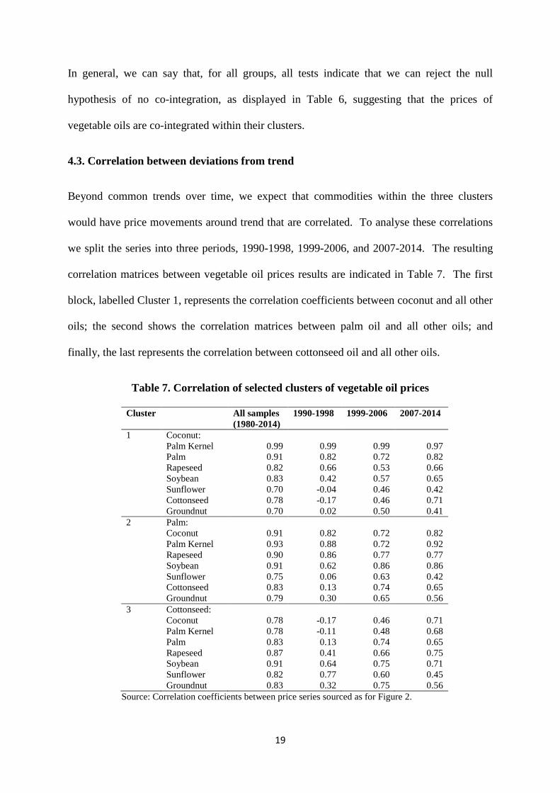
4.3. Correlation between deviations from trend
Beyond common trends over time, we expect that commodities within the three clusters
would have price movements around trend that are correlated. To analyse these correlations
we split the series into three periods, 1990-1998, 1999-2006, and 2007-2014. The resulting
correlation matrices between vegetable oil prices results are indicated in Table 7. The first
block, labelled Cluster 1, represents the correlation coefficients between coconut and all other
oils; the second shows the correlation matrices between palm oil and all other oils; and
finally, the last represents the correlation between cottonseed oil and all other oils.
Table 7. Correlation of selected clusters of vegetable oil prices
Cluster All samples (1980-2014)
1990-1998 1999-2006 2007-2014
1 Coconut: Palm Kernel 0.99 0.99 0.99 0.97 Palm 0.91 0.82 0.72 0.82 Rapeseed 0.82 0.66 0.53 0.66 Soybean 0.83 0.42 0.57 0.65 Sunflower 0.70 -0.04 0.46 0.42 Cottonseed 0.78 -0.17 0.46 0.71 Groundnut 0.70 0.02 0.50 0.41 2 Palm: Coconut 0.91 0.82 0.72 0.82 Palm Kernel 0.93 0.88 0.72 0.92 Rapeseed 0.90 0.86 0.77 0.77 Soybean 0.91 0.62 0.86 0.86 Sunflower 0.75 0.06 0.63 0.42 Cottonseed 0.83 0.13 0.74 0.65 Groundnut 0.79 0.30 0.65 0.56 3 Cottonseed: Coconut 0.78 -0.17 0.46 0.71 Palm Kernel 0.78 -0.11 0.48 0.68 Palm 0.83 0.13 0.74 0.65 Rapeseed 0.87 0.41 0.66 0.75 Soybean 0.91 0.64 0.75 0.71 Sunflower 0.82 0.77 0.60 0.45 Groundnut 0.83 0.32 0.75 0.56
Source: Correlation coefficients between price series sourced as for Figure 2.

20
In general, we can see that the deviations from trends have become more correlated over
time. In 1990-1998, some vegetable oils were found to be negatively correlated. While in
2007-2014, most of them are found to be highly correlated.2 The complete correlation matrix
is presented in Table A2.1 (Appendix A2).
5. Dependence of vegetable oil markets on energy markets, financial volatility and
overall economic performance
Here we set out to model the price behaviour of the vegetable oils at the level of the three
clusters. From section 4.2, we note the co-integration of vegetable oils within these clusters
and so we take the average price of clustered vegetable oils weighted by their shares within
the clusters. This gives us three cluster price series, to which we assign the titles: VO1, VO2
and VO3. VO1 represents vegetable oil prices in Cluster 1, comprising coconut and palm
kernel oils. VO2 represents Cluster 2, which includes palm, rapeseed, soybean and sunflower
oils. The VO3 is Cluster 3, comprising cottonseed and groundnut oils. Our objective is to
find a long run relationship between the clustered oil prices, the petroleum price and variables
that indicate financial and real demand shocks. As a financial indicator we use the US 10
year bond rate, which might be seen as representing the yields on global long term assets and
hence the opportunity cost of storing commodities that include the vegetable oils. For
indicators of real demand we include the levels of GDP in selected countries. All variables
are then incorporated into a Vector Error Correction Model (VECM).
5.1 Data and pre-tests
Similar to our previous analysis, we use quarterly data from 1980-Q1 to 2014-Q4 for
clustered average vegetable oil prices (VO1, VO2, VO3), the petroleum price, the 10 year US
bond rate and the GDP levels of China, the EU-15, India and the U.S. Data of petroleum 2 Although these results are not shown in the table, minor exceptions include the correlation coefficients between the prices of sunflower oil and other oils and between groundnut oil and other oils.

21
price is obtained from (IMF, 2015a). We use the simple average of the Brent, Dubai and
West Texas prices. The data is expressed as average quarterly prices in US$ per barrel. Data
for GDPs are obtained from World Economic Outlook Database (WEOD) (IMF, 2015b).
Since all GDP data are presented annually, we interpolate the series into quarterly data using
GDP shares from OECD-Stat (2015) for U.S, EU-15 and India. For China, the quarterly
GDP shares are obtained from National Bureau of Statistics of China (NBS, 2015). Data for
10-year U.S bond rate is taken from Federal Reserve Bank of St. Louis (FRED, 2015). The
summary statistics of the series are available in Table 8. A preliminary assessment is
possible from a plot of the prices of each vegetable oil cluster with petroleum prices, which
shows the common movement indicated by Figure 8.
Table 8. Summary statistics for vegetable oil clusters, EU-15 GDP, US GDP and US-Bond rate
Oil Mean Standard deviation
Skewness Kurtosis Observation
VO1 6.44 0.42 0.29 3.04 140 VO2 6.32 0.36 0.65 2.88 140 VO3 6.74 0.35 0.69 2.98 140 Petroleum 3.46 0.66 0.59 2.12 140 US-Bond rate 1.76 0.52 -0.32 2.57 140 China- GDP 5.62 1.17 0.52 2.00 140 EU-15- GDP 7.46 0.58 -0.46 2.12 140 India-GDP 4.83 0.75 0.59 2.02 140 US GDP 7.62 0.53 -0.32 1.90 140
Data source: IMF (2015a), UNCTADSTAT (2015), and World-Bank (2015) . Nominal GDPs are reported in billion US$ and obtained from (IMF, 2015b). The US-Bond is obtained from FRED (2015), based on quarterly 10 year Bond in percentage. Note: all series are presented in natural logarithm (ln).
Before we move to the VECM, unit root and co-integration tests are employed to seek
whether there is long run co-integration among the series. As before, we employ three unit
root tests, namely, the ADF, the PP, and the KPSS tests. Based on those tests, the series are
generally found to be I(1). For the series of VO1 and VO3, the ADF test indicates that these
series are stationery at 5% significant level. Yet both the PP and KPSS results indicate non-

22
stationarity. For 10 year US-Bond rate, the KPSS test suggests that we cannot reject the null
hypothesis of stationarity, since the KPSS shows a non-significant statistics; however, for
both ADF and PP we cannot reject the unit root hypothesis.
Figure 8. Vegetable oil cluster and petroleum prices
Data source: IMF (2015a), UNCTADSTAT (2015), and World-Bank (2015) . * Indices are author’s calculation (1980q1=1).
As before, our next step is to investigate whether there exists a long run relationship between
these variables. Johansen tests are again employed. We compute the co-integrating
relationship based on trace statistics, max-eigenvalue statistics and SBIC and HQIC. The
results are included in Table 10. For each test, we find that there exists at least one co-
integrating vector.
5.2. The VECM specification
Since all variables are found to be co-integrated, our next step is to estimate the VECM. A
VECM has two parts, the first part, in the parenthesis, indicates the long-run relationship
0
20
40
60
80
100
120
140
1980
Q1
1981
Q1
1982
Q1
1983
Q1
1984
Q1
1985
Q1
1986
Q1
1987
Q1
1988
Q1
1989
Q1
1990
Q1
1991
Q1
1992
Q1
1993
Q1
1994
Q1
1995
Q1
1996
Q1
1997
Q1
1998
Q1
1999
Q1
2000
Q1
2001
Q1
2002
Q1
2003
Q1
2004
Q1
2005
Q1
2006
Q1
2007
Q1
2008
Q1
2009
Q1
2010
Q1
2011
Q1
2012
Q1
2013
Q1
2014
Q1
Petroleum
VO 1
VO 2
VO 3

23
between variables, while the second part, stated in difference terms, indicates the short-run
deviation from the equilibrium. The fully specified model can be written as follows:
1 1
1 1 1
1 1 1 11 1 2 2 3 3 1 11
1 1 1 1 11
1 1 1 1 11 1 1 1 1
1 2 31 1 1 1 1
t t
t t t
t i t i t i t i
t t PO t Ch Cht
EU EU Ind Ind US US r t
p p p p p
i i i i ii i i i i
VO VO VO PO YVO
Y Y Y r c
VO VO VO PO
β β β βα
β β β β
µ σ ϑ λ γ
− −
− − −
− − − −
− − −
−
− − − − −
= = = = =
+ + + + ∆ = + + + + +
+ ∆ + ∆ + ∆ + ∆ +∑ ∑ ∑ ∑1 1 1 1
1 1 1 1 1 1
1 1 1 1 + (1)
t i t i t i t i
t i
p p p p
i Ch i EU i Ind i US ti i i i
r
Y Y Y Y cθ t r ω ε− − − −
−
− − − −
= = = =
∆
+ ∆ ∆ + ∆ + ∆ + +
∑
∑ ∑ ∑ ∑
1 1
1 1 1
2 2 2 22 1 1 1 3 3 1 12
2 1 1 1 11
1 1 1 1 12 2 2 2 2
1 2 31 1 1 1 1
t t
t t t
t i t i t i t i
t t PO t Ch Cht
EU EU Ind Ind US US r t
p p p p p
i i i i ii i i i i
VO VO VO PO YVO
Y Y Y r c
VO VO VO PO
β β β βα
β β β β
µ σ ϑ λ γ
− −
− − −
− − − −
− − −
−
− − − − −
= = = = =
+ + + + ∆ = + + + + +
+ ∆ + ∆ + ∆ + ∆ +∑ ∑ ∑ ∑1 1 1 1
2 2 2 2 2 2
1 1 1 1 + (2)
t i t i t i t i
t i
p p p p
i Ch i EU i Ind i US ti i i i
r
Y Y Y Y cθ t r ω ε− − − −
−
− − − −
= = = =
∆
+ ∆ ∆ + ∆ + ∆ + +
∑
∑ ∑ ∑ ∑
1 1
1 1 1
3 3 3 33 1 1 1 2 2 1 13
3 3 3 3 31
1 1 1 1 13 3 3 3 3
1 2 31 1 1 1 1
t t
t t t
t i t i t i t i
t t PO t Ch Cht
EU EU Ind Ind US US r t
p p p p p
i i i i ii i i i i
VO VO VO PO YVO
Y Y Y r c
VO VO VO PO
β β β βα
β β β β
µ σ ϑ λ γ
− −
− − −
− − − −
− − −
−
− − − − −
= = = = =
+ + + + ∆ = + + + + +
+ ∆ + ∆ + ∆ + ∆ +∑ ∑ ∑ ∑1 1 1 1
3 3 3 3 3 3
1 1 1 1 + (3)
t i t i t i t i
t i
p p p p
i Ch i EU i Ind i US ti i i i
r
Y Y Y Y cθ t r ω ε− − − −
−
− − − −
= = = =
∆
+ ∆ ∆ + ∆ + ∆ + +
∑
∑ ∑ ∑ ∑
Where, itVO represents the clustered vegetable oil prices from Cluster i. This means that
itVO∆ , on the left hand side of the models, indicates the difference in vegetable oil prices
between quarters and the equations indicate how this difference is apportioned between the
continuing long run relationship and short term responses to shocks. Also, PO represents the
petroleum price; kY represents the GDP level for region k; and r is interest rate. The β s are
co-integrating coefficients linking each dependent variable to the long-run relationship.
, , , , , , ,µ σ δ λ γ θ t r and ω are the short-run coefficients, and α is called the adjustment

24
parameter. It indicates the speed of short run adjustment departures from the long run
relationship between the variables. The larger the level of α , the faster the dependent
variable responses to deviations from the long-run “equilibrium” path. We are particularly
interested in α and β since they indicate how the model responds to the deviations from the
long run equilibrium in term of direction and speed. Note that all variables are computed in
natural logarithms (ln).
Table 9. Unit root tests for GDPs and US 10 year bond
Series ADF PP KPSS levels lnVO1(2) -3.87* -3.32 0.36** lnVO2(2) -3.04 -2.67 0.54** lnVO3(2) -3.98* -3.22 0.41** lnChina(5) -1.98 -2.13 0.54** lnEU15(1) -1.60 -1.62 0.66** lnIndia(1) -1.27 -1.24 1.55** lnUS(7) -1.13 -0.83 0.40** lnUS-bond(10) -2.35 -3.27 0.10 lnPetroleum(3) -2.52 -2.28 0.76** First differences lnVO1(1) -6.78** -7.58** 0.03 lnVO2(1) -7.31** -8.52** 0.04 lnVO3(1) -7.09** -7.22** 0.03 lnChina(4) -4.64** -23.61** 0.02 lnEU15(4) -4.11** -11.59** 0.08 lnIndia(0) -11.59** -9.34** 0.03 lnUS(5) -5.92** -13.66** 0.03 lnUS-bond(2) -6.10** -9.43** 0.02 lnPetroleum(2) -6.70** -9.28** 0.05
Numbers of lags selected are in the parenthesis. *(**) indicates significant level at 5%(1%).
As stated earlier, the term in the parentheses indicates long run relationship. The first
coefficients in the long run relationships are normalised to one. Here, we report the VECM
results for VO2 which is the most economically significant group of vegetable oils. It
indicates the behaviour of the collective prices of palm, rapeseed, soybean and sunflower oils.
For VO2, the long-run relationship based on our model can be written as:

25
1 1 1 1
*** *** *** *** ***2 1 1 3 1 1
***0.65 0.26 0.17 0.57 0.19 0.36
(0.07) (0.09) (0.05) (0.10) (0.07) (0.t t t tt t t Ch EU IndVO VO VO PO Y Y Y− − − −− − −= + + − + +
1
***1
12) 0.12 0.53 1.88 (4)
(0.11) (0.86)
tUS tY r− −− +−
The more complete results can be found in Appendix A3. In this model, we use 5 lags, as
specified by AIC in our lag-order selection tests (see table A1.2 in Appendix A1). Our
samples are quarterly, from 1980Q1 to 2014Q4.
Table 10. Johansen co-integration tests for groups of vegetable oils, petroleum, US 10-year bond, and four countries GDPs.
Max rank
Trace statistic
1% critical value
Max statistic
1% critical value
SBIC HQIC
0 270.53 204.95 82.74 62.80 -18.47* -22.72 1 187.79 168.36 56.77** 57.69 -18.46 -22.93 2 131.02** 133.57 50.09 51.57 -18.34 -23.00 3 80.93 103.18 25.50 45.10 -18.24 -23.06* 4 55.44 76.07 20.84 38.77 -18.02 -22.99 5 34.60 54.46 18.89 32.24 -17.85 -22.94 6 16.71 35.65 11.32 25.52 -17.74 -22.91 7 4.38 20.04 4.36 18.63 -17.64 -22.88 8 0.02 6.65 0.0.02 6.65 -17.56 -22.84 9 -17.53 -22.82
**Trace and max statistics indicate significant level at 1%, number of lags = 5.
The results show that in the long run, the price of VO2 responds positively to other vegetable
oil prices. When VO1 and VO3 prices increase by US$1, the VO2 price rises by 65 U.S cents
and 26 U.S cents, respectively, in the long run. Similarly, an increase by US$1 of the
petroleum price is associated with a long run increase of 17 U.S cents in the VO2 price. For
GDPs, the VO2 price is found to respond positively to GDP in India and EU-15. As expected,
since the interest rate represents the opportunity cost of storage, we find that the VO2 price is
negatively correlated with the interest rate in the long-run: a one percent increase in the 10-
year US bond rate decreases the VO2 price by 0.53 US cents. This implies that as interest

26
rates fall, and so yields on financial assets decrease, the storable commodities become more
attractive investment relative to financial assets.
The adjustment parameter for 2VO∆ or 2α is equal to -0.27 and the estimate is statistically
significant. This means that when the level of the VO2 price is $1 above its long-run
equilibrium, the next quarter will yield a 27 cents decline, other thing equal. The full
dynamics of the model yield a good fit for the VO2 price within the estimation interval, as
indicated in Figure 9.
Figure 9. Actual and fitted values of VO2 based on VECM
6. Forward simulations: petroleum price movements, financial tightening and growth
In the period beyond our estimation interval the petroleum price has been volatile with a
tendency to decline. At the same time, financial markets have been very liquid with
tightening foreshadowed, at least in the US while comparatively rapid growth has continued
in Asian regions that are active in the vegetable oil trade, such as India and China. In this
section we use the estimated model to simulate beyond the estimation interval, to 2020, with
a view to examining the implications of future shocks such as these for vegetable oil markets.
0
200
400
600
800
1000
1200
1400
1600
1980
Q1
1981
Q2
1982
Q3
1983
Q4
1985
Q1
1986
Q2
1987
Q3
1988
Q4
1990
Q1
1991
Q2
1992
Q3
1993
Q4
1995
Q1
1996
Q2
1997
Q3
1998
Q4
2000
Q1
2001
Q2
2002
Q3
2003
Q4
2005
Q1
2006
Q2
2007
Q3
2008
Q4
2010
Q1
2011
Q2
2012
Q3
2013
Q4
Actual
Fitted

27
For this purpose, we use the estimated parameters in equations (1)-(3) to solve for the future
paths of VO1, VO2 and VO3 while setting as exogenous in turn the petroleum price, PO, the
US 10-year Bond rate, r, and the growth paths of regional GDP, Yk. A baseline scenario is
constructed in which it is assumed that the petroleum price stabilises at $50 per barrel beyond
2015Q4, the US long bond rate stabilises at 2 percent after 2015Q3 and nominal GDP levels
are as projected in the IMF’s World Economic Outlook (IMF, 2015b). The paths of the
petroleum price and interest rate in base line projection are presented in Figure 10.
Figure 10. Petroleum Price and Interest Rate Shocks in Baseline Scenario
Source: Fitted values and forward simulations of the model described in the text.
To compare with this baseline, we propose three scenarios that embody shocks to the
petroleum price, the interest rate and to the path of Indian GDP. We consider Indian growth
since it is the largest importer of vegetable oils (USDA-FAS, 2015c). In each case we
consider two versions embodying a positive and a negative shock. First, we imagine that the
petroleum price will either recover and stabilise at $100 a barrel or fall to $25 a barrel after
2015Q4. Second, we suppose that the US 10-year bond rate will alternately recover to four
per cent or remain at two per cent after 2015Q3. And, finally, we consider the extreme
possibilities that Indian GDP will grow by either 15 per cent or four per cent per year after
0.00
2.00
4.00
6.00
8.00
10.00
12.00
14.00
16.00
0
20
40
60
80
100
120
140
1980
Q1
1981
Q3
1983
Q1
1984
Q3
1986
Q1
1987
Q3
1989
Q1
1990
Q3
1992
Q1
1993
Q3
1995
Q1
1996
Q3
1998
Q1
1999
Q3
2001
Q1
2002
Q3
2004
Q1
2005
Q3
2007
Q1
2008
Q3
2010
Q1
2011
Q3
2013
Q1
2014
Q3
2016
Q1
2017
Q3
2019
Q1
2020
Q3
Petroleum-Base
10-year US Bond rate-Base

28
2014Q4. The exogenous projections based on these three scenarios are plotted in Figure
11(a) to Figure 11(c).
Figure 11. Exogenous Shocks in Forecast
0
20
40
60
80
100
120
14019
80Q
119
81Q
319
83Q
119
84Q
319
86Q
119
87Q
319
89Q
119
90Q
319
92Q
119
93Q
319
95Q
119
96Q
319
98Q
119
99Q
320
01Q
120
02Q
320
04Q
120
05Q
320
07Q
120
08Q
320
10Q
120
11Q
320
13Q
120
14Q
320
16Q
120
17Q
320
19Q
120
20Q
3
(a) Petroleum scenario
Petroleum-ActualPetroleum-$25Petroleum+$100
0.00
2.00
4.00
6.00
8.00
10.00
12.00
14.00
16.00
1980
Q1
1981
Q4
1983
Q3
1985
Q2
1987
Q1
1988
Q4
1990
Q3
1992
Q2
1994
Q1
1995
Q4
1997
Q3
1999
Q2
2001
Q1
2002
Q4
2004
Q3
2006
Q2
2008
Q1
2009
Q4
2011
Q3
2013
Q2
2015
Q1
2016
Q4
2018
Q3
2020
Q2
(b) Interest Rate Scenario
US Bond Rate-Actual
US Bond rate +4%
US Bond rate-1.5%
0100200300400500600700800900
1000
1980
Q1
1981
Q4
1983
Q3
1985
Q2
1987
Q1
1988
Q4
1990
Q3
1992
Q2
1994
Q1
1995
Q4
1997
Q3
1999
Q2
2001
Q1
2002
Q4
2004
Q3
2006
Q2
2008
Q1
2009
Q4
2011
Q3
2013
Q2
2015
Q1
2016
Q4
2018
Q3
2020
Q2
(c) Indian GDP scenario
India-4%
India+15%
India-Actual

29
The simulation results for VO2 prices are shown in Figure 12 to Figure 14. The petroleum
pricing scenarios are illustrated in Figure 12. The results show the expected sign but
relatively little sensitivity of the future path of VO2 prices to the petroleum price. A
petroleum price recovery to $100 per barrel would yield a VO2 price level just 10 percent
higher than when the petroleum price falls to $25 per barrel.
Figure 12. Forecast of VO2 prices based on petroleum price scenario
The interest rate shocks cause a larger VO2 price gap, as between the recovery of the rate to
four per cent and its stagnation at two per cent. These results are shown in Figure 13. The
VO2 price difference between both shocks is around 60 percent. The sign is as expected, with
the higher bond yield discouraging storage demand and causing a lower VO2 price level. This
result supports the thesis that the price of VO2 is now highly responsive to financial market
volatility, or that these commodity markets have become “financialised” in the last two
decades.
0
200
400
600
800
1000
1200
1400
Actual
Fitted
Base
Petroleum+$100
Petroleum-$25

30
Figure 13 Forecast of VO2 prices based on interest rate scenario
Finally, the third scenario projects the differences in VO2 prices when we set Indian GDP to
grow by 15 percent and 4 percent, as plotted in Figure 14. As expected, the projections show
that VO2 will have higher equilibrium price under the more optimistic Indian growth scenario.
This result is consistent with the long run relationship result in Equation (4). The price of
VO2 will reach its steady state in 2016Q3 onward with an average difference of 17 percent
between the low and high growth cases.
7. Conclusion
The markets for vegetable oils have expanded significantly in recent decades in association
with the diversification in their use across final consumption as food, industrial applications
and substitution as fuels for petroleum derivatives. Global markets for such products have
integrated and volatility has increased with the increased prominence of financial
determinants of demand for storable commodities. Research to date shows the evolution of
vegetable oil markets in these directions as later studies find increasing roles for energy
products and financial variables in determining the paths of vegetable oil prices. We test
extensively for changes in the level of integration of these markets through time, examining
0
200
400
600
800
1000
1200
1400
Actual
Fitted
Base
Bond+4%
Bond-1.5%

31
both common trends and co-movements around trend, finding it most useful to aggregate
vegetable oils into three clusters, the second of which is the largest, dominated by palm oil.
Figure 14 Forecast of VO2 prices based on Indian GDP scenario
We then examine the dependence of average prices in these clusters on changes in the
petroleum price, financial liquidity and economic growth in the largest vegetable oil importer,
namely India. Scenarios for market behaviour in response to slow global growth, low energy
prices and tighter monetary policy show strong sensitivity, in the expected direction, to the
interest rate, intermediate sensitivity to Indian aggregate demand and relatively weak
sensitivity to the petroleum price, albeit in the anticipated direction.
0
200
400
600
800
1000
1200
1400
Actual
Fitted
Base
India+15%
India-4%

32
References
ABDEL, H. & ARSHAD, F. The impact of petroleum prices on vegetable oils prices: evidence from cointegration tests. International Borneo Business Conference on Global Changes, Malaysia, 2008.
AMIRUDDIN, M. N., RAHMAN, A. K. A. & SHARIFF, F. 2005. Market potential and challenges for the Malaysian palm oil industry in facing competition from other vegetable oils. Oil palm industry economic journal 5, 17-27.
BAFFES, J. 2011. The energy/non-energy price link: channels, issues and implications. Methods to Analyse Agricultural Commodity Price Volatility. Springer.
Baffes J and T Haniotis (2016). 'What explains agricultural price movements?' World Bank Policy Research working Paper 7589. World Bank, Washington D.C.
BPS 2006. Indonesia's input output table 2005, Jakarta, Badan Pusat Statistik. BPS 2009. Table input output Indonesia: updating 2008 (Indonesian input output table),
Jakarta, Badan Pusat Statistik. CAMPICHE, J. L., BRYANT, H. L., RICHARDSON, J. W. & OUTLAW, J. L. Examining
the evolving correspondence between petroleum prices and agricultural commodity prices. The American Agricultural Economics Association Annual Meeting, Portland, OR, 2007.
CIAIAN, P. 2011. Interdependencies in the energy–bioenergy–food price systems: A cointegration analysis. Resource and energy economics, 33, 326-348.
DOSM 2014. Malaysia: annual gross domestic product 2005-2013, Department of statistics, Malaysia.
FRED. 2015. Economic data [Online]. St. Louis: Federal Reserve Bank of St. Louis. Available: https://research.stlouisfed.org/fred2/ [Accessed 18 March 2015.
GERASIMCHUK, I. & KOH, P. Y. 2013. The EU biofuel policy and palm oil: Cutting subsidies or cutting rainforest? The International Institute for Sustainable Development, Geneva, Switzerland,(http://www. iisd. org/gsi/sites/default/files/bf_eupalmoil. pdf).
GRIFFITH, G. & MEILKE, K. D. 1979. Relationships among North American fats and oils prices. American Journal of Agricultural Economics, 61, 335-341.
HARRI, A., NALLEY, L. & HUDSON, D. 2009. The relationship between oil, exchange rates, and commodity prices. Journal of Agricultural and Applied Economics, 41, 501-510.
HASSOUNEH, I., SERRA, T., GOODWIN, B. K. & GIL, J. M. 2012. Non-parametric and parametric modeling of biodiesel, sunflower oil, and crude oil price relationships. Energy Economics, 34, 1507-1513.
IMF. 2015a. IMF Primary Commodity Prices [Online]. International Monetary Fund. Available: http://www.imf.org/external/np/res/commod/index.aspx [Accessed 18 March 2015.
IMF. 2015b. World Economic Outlook Database [Online]. International Monetary Fund. Available: http://www.imf.org/external/pubs/ft/weo/2014/02/weodata/index.aspx [Accessed 11 November 2015.
IN, F. & INDER, B. 1997. Long‐run Relationships Between World Vegetable Oil Prices. Australian journal of agricultural and resource economics, 41, 455-470.
MITCHELL, D. 2008. A note on rising food prices. World Bank Policy Research Working Paper Series, 4682.
NAZLIOGLU, S., ERDEM, C. & SOYTAS, U. 2013. Volatility spillover between oil and agricultural commodity markets. Energy Economics, 36, 658-665.

33
NAZLIOGLU, S. & SOYTAS, U. 2012. Oil price, agricultural commodity prices, and the dollar: A panel cointegration and causality analysis. Energy Economics, 34, 1098-1104.
NBS. 2015. National Data [Online]. National Bureau of Statistics of China. Available: http://data.stats.gov.cn/english/easyquery.htm?cn=B01 [Accessed 11 November 2015.
OECD-STAT. 2015. Quarterly national accounts: historical GDP expenditure approach [Online]. Organisation for economic co-operation and development. Available: http://stats.oecd.org/index.aspx?queryid=350 [Accessed 2 November 2015 2015].
Ohashi K, Okimoto T. (2016), "Increasing trends in the excess comovement of commodity prices", ANU CAMA Working Paper, Canberra, February.
OWEN, A., CHOWDHURY, K. & GARRIDO, J. 1997. Price interrelationships in the vegetable and tropical oils market. Applied economics, 29, 119-124.
OWEN, A. D., CHOWDHURY, K. & GARRIDO, J. 1996. A market share model for vegetable and tropical oils. Applied Economics Letters, 3, 95-99.
PERI, M. & BALDI, L. 2010. Vegetable oil market and biofuel policy: an asymmetric cointegration approach. Energy Economics, 32, 687-693.
REBOREDO, J. C. 2012. Do food and oil prices co-move? Energy policy, 49, 456-467. SANDERS, D. J., BALAGTAS, J. V. & GRUERE, G. 2014. Revisiting the palm oil boom in
South-East Asia: fuel versus food demand drivers. Applied economics, 46, 127-138. SERRA, T. 2011. Volatility spillovers between food and energy markets: a semiparametric
approach. Energy Economics, 33, 1155-1164. UNCTADSTAT. 2015. Free market commodity prices [Online]. United Nations Conference
on Trade and Development. Available: http://unctadstat.unctad.org/wds/TableViewer/tableView.aspx?ReportId=28768.
USDA-FAS 2015. EU Biofuels Annual 2015. GAIN Report Number: NL5028. USDA-FAS. 2015a. New Crop U.S Soybean Sales Fall on Surging Spunth American
Exports. Oilseeds: World Markets and Trade [Online], August 2015. Available: http://apps.fas.usda.gov/psdonline/circulars/oilseeds.pdf [Accessed 21 August 2015].
USDA-FAS. 2015b. Production, supply, and distribution online [Online]. United States Department of Agriculcure- Foreign Agricultural Service. Available: http://apps.fas.usda.gov/psdonline/psdQuery.aspx [Accessed 19 August 2015.
USDA-FAS. 2015c. Pakistan Oilseed Processors Seize Opportunity to Crush Soybeans. Oilseeds: world markets and trade [Online], December 2015. Available: http://apps.fas.usda.gov/psdonline/circulars/oilseeds.pdf [Accessed 5 January 2016].
WITS. 2015. Trade data (UN Comtrade) [Online]. World Integrated Trade Solusion Available: http://wits.worldbank.org/WITS/WITS/AdvanceQuery/RawTradeData/QueryDefinition.aspx?Page=RawTradeData [Accessed 11 February 2015.
WORLD-BANK. 2015. Commodity markets [Online]. Available: http://econ.worldbank.org/WBSITE/EXTERNAL/EXTDEC/EXTDECPROSPECTS/0,,contentMDK:21574907~menuPK:7859231~pagePK:64165401~piPK:64165026~theSitePK:476883,00.html [Accessed 21 August 2015.
YU, T.-H., BESSLER, D. A. & FULLER, S. Cointegration and causality analysis of world vegetable oil and crude oil prices. The American Agricultural Economics Association Annual Meeting, Long Beach, California, 2006. 23-26.
ZHANG, Z., LOHR, L., ESCALANTE, C. & WETZSTEIN, M. 2010. Food versus fuel: What do prices tell us? Energy policy, 38, 445-451.
ZHOU, A. & THOMSON, E. 2009. The development of biofuels in Asia. Applied energy, 86, S11-S20.

34
Appendices
Appendix A1. Lag Order Selection
Table A1.1. Lag-order selection of vegetable oils
Group Lag AIC HQIC SBIC Coconut/Palm Kernel 0 -1.68 -1.66 -1.63
1 -4.44 -4.38 -4.31 2 -4.74* -4.65* -4.52* 3 -4.70 -4.58 -4.40 4 -4.68 -4.52 -4.29
Palm/Rapeseed/ Soybean/Sunflower
0 -1.78 -1.74 -1.69 1 -7.43 -7.26 -7.01* 2 -7.76 -7.45* -6.99 3 -7.81* -7.36 -6.70 4 -7.75 -7.16 -6.29
Cottonseed/Groundnut 0 0.41 0.43 0.45 1 -2.94 -2.88 -2.81 2 -3.34* -3.26* -3.13* 3 -3.32 -3.20 -3.02 4 -3.27 -3.11 -2.89
Table A1.2. Lag-order selection of vegetable oil clusters, GDPs , Petroleum and interest rate
Lag AIC HQIC SBIC 0 -3.77 -3.69 -3.57 1 -24.91 -24.11* -22.95* 2 -25.55 -24.03 -21.81 3 -25.50 -23.26 -19.99 4 -26.26 -23.31 -18.99 5 -26.44* -22.77 -17.40 6 -26.36 -21.97 -15.55
Note: here we proceed with 5-lag since 1-lag VECM will produce no short term dynamics.

35
Appendix A2. Correlation Matrix
Table A2.1 Correlation matrix of vegetable oil prices
All samples | lnCocN lnCotN lnGroN lnPalN lnPkerN lnRapN lnSoyN lnSunN -------------+------------------------------------------------------------------------ lnCocN | 1.0000 lnCotN | 0.7793 1.0000 lnGroN | 0.7011 0.8326 1.0000 lnPalN | 0.9074 0.8304 0.7929 1.0000 lnPkerN | 0.9898 0.7755 0.7020 0.9269 1.0000 lnRapN | 0.8239 0.8693 0.8829 0.8985 0.8260 1.0000 lnSoyN | 0.8297 0.9107 0.8820 0.9076 0.8326 0.9439 1.0000 lnSunN | 0.6970 0.8220 0.8470 0.7491 0.6915 0.8855 0.8725 1.0000 1990-1998 | lnCocN lnCotN lnGroN lnPalN lnPkerN lnRapN lnSoyN lnSunN -------------+------------------------------------------------------------------------ lnCocN | 1.0000 lnCotN | -0.1704 1.0000 lnGroN | 0.0283 0.3212 1.0000 lnPalN | 0.8209 0.1324 0.3040 1.0000 lnPkerN | 0.9895 -0.1102 0.0665 0.8766 1.0000 lnRapN | 0.6603 0.4099 0.5924 0.8625 0.7158 1.0000 lnSoyN | 0.4246 0.6393 0.6538 0.6220 0.4758 0.8724 1.0000 lnSunN | -0.0434 0.7728 0.2657 0.0594 -0.0175 0.3859 0.5858 1.0000 1999-2006 | lnCocN lnCotN lnGroN lnPalN lnPkerN lnRapN lnSoyN lnSunN -------------+------------------------------------------------------------------------ lnCocN | 1.0000 lnCotN | 0.4585 1.0000 lnGroN | 0.4996 0.7515 1.0000 lnPalN | 0.7180 0.7434 0.6529 1.0000 lnPkerN | 0.9912 0.4843 0.5085 0.7201 1.0000 lnRapN | 0.5305 0.6602 0.7462 0.7668 0.5472 1.0000 lnSoyN | 0.5716 0.7515 0.7833 0.8587 0.5830 0.8867 1.0000 lnSunN | 0.4609 0.6012 0.6436 0.6264 0.5144 0.8414 0.6939 1.0000 2007-2014 | lnCocN lnCotN lnGroN lnPalN lnPkerN lnRapN lnSoyN lnSunN -------------+------------------------------------------------------------------------ lnCocN | 1.0000 lnCotN | 0.7112 1.0000 lnGroN | 0.4073 0.5580 1.0000 lnPalN | 0.8230 0.6490 0.5644 1.0000 lnPkerN | 0.9652 0.6772 0.4005 0.9156 1.0000 lnRapN | 0.6555 0.7450 0.8292 0.7725 0.6782 1.0000 lnSoyN | 0.6510 0.7101 0.8288 0.8645 0.7151 0.9308 1.0000 lnSunN | 0.4179 0.4550 0.7000 0.4186 0.3865 0.6019 0.6876 1.0000

36
Appendix 3. VECM Estimation
. vec lnVO2N lnVO1N lnVO3N lagPet2 lnUSBond lnEU15 lnChina lnIndia lnUS, trend(constant) lags(5) Vector error-correction model Sample: 1981q4 - 2014q4 No. of obs = 133 AIC = -25.97841 Log likelihood = 2077.564 HQIC = -22.88755 Det(Sigma_ml) = 2.19e-25 SBIC = -18.37223 Equation Parms RMSE R-sq chi2 P>chi2 ---------------------------------------------------------------- D_lnVO2N 38 .086936 0.4719 84.88455 0.0000 D_lnVO1N 38 .126114 0.5122 99.75126 0.0000 D_lnVO3N 38 .088138 0.5163 101.4082 0.0000 D_lagPet2 38 .117814 0.5263 105.5533 0.0000 D_lnUSBond 38 .080083 0.3833 59.04685 0.0159 D_lnEU15 38 .046602 0.4170 67.95338 0.0020 D_lnChina 38 .051507 0.8633 600.0474 0.0000 D_lnIndia 38 .035682 0.4747 85.84707 0.0000 D_lnUS 38 .007428 0.8768 676.293 0.0000 ---------------------------------------------------------------- ------------------------------------------------------------------------------ | Coef. Std. Err. z P>|z| [95% Conf. Interval] -------------+---------------------------------------------------------------- D_lnVO2N | _ce1 | L1. | -.2706113 .1318761 -2.05 0.040 -.5290838 -.0121389 | lnVO2N | LD. | .1705194 .1666658 1.02 0.306 -.1561396 .4971783 L2D. | .1815241 .176581 1.03 0.304 -.1645682 .5276165 L3D. | -.0833865 .1729533 -0.48 0.630 -.4223687 .2555957 L4D. | .1270943 .1703914 0.75 0.456 -.2068667 .4610553 | lnVO1N | LD. | .2745382 .0963722 2.85 0.004 .0856522 .4634242 L2D. | -.2463305 .1082236 -2.28 0.023 -.4584449 -.034216 L3D. | -.0158286 .1053126 -0.15 0.881 -.2222374 .1905802 L4D. | -.1311863 .1046835 -1.25 0.210 -.3363622 .0739897 | lnVO3N | LD. | -.0834592 .1342718 -0.62 0.534 -.3466271 .1797088 L2D. | .1444412 .1540622 0.94 0.348 -.1575151 .4463974 L3D. | .1314982 .1593784 0.83 0.409 -.1808778 .4438742 L4D. | -.1298623 .1351008 -0.96 0.336 -.394655 .1349305 | lagPet2 | LD. | -.1392295 .0789369 -1.76 0.078 -.2939431 .015484 L2D. | .106571 .0789773 1.35 0.177 -.0482218 .2613637 L3D. | -.0059141 .0674728 -0.09 0.930 -.1381583 .1263301 L4D. | .025098 .0650008 0.39 0.699 -.1023012 .1524972 | lnUSBond | LD. | -.1100746 .115561 -0.95 0.341 -.33657 .1164208 L2D. | .0269665 .1224302 0.22 0.826 -.2129922 .2669252 L3D. | .3128704 .1272368 2.46 0.014 .0634909 .5622499 L4D. | -.0395873 .1281395 -0.31 0.757 -.290736 .2115615 | lnEU15 | LD. | -.0868763 .1818955 -0.48 0.633 -.4433849 .2696322 L2D. | -.0943033 .178613 -0.53 0.598 -.4443784 .2557718 L3D. | -.1138882 .1680692 -0.68 0.498 -.4432978 .2155215 L4D. | -.1764041 .1750892 -1.01 0.314 -.5195726 .1667645 | lnChina | LD. | .1340802 .1484421 0.90 0.366 -.156861 .4250214 L2D. | .2177731 .1414548 1.54 0.124 -.0594732 .4950194 L3D. | -.0977825 .1431962 -0.68 0.495 -.3784418 .1828769 L4D. | .0139323 .1455422 0.10 0.924 -.2713252 .2991899 | lnIndia |

37
LD. | .0130594 .2335084 0.06 0.955 -.4446086 .4707273 L2D. | .2093605 .2350784 0.89 0.373 -.2513846 .6701057 L3D. | .9297763 .2388856 3.89 0.000 .461569 1.397984 L4D. | .2299029 .2541275 0.90 0.366 -.268178 .7279837 | lnUS | LD. | .5452754 1.139104 0.48 0.632 -1.687328 2.777879 L2D. | -.7041424 1.091008 -0.65 0.519 -2.842479 1.434194 L3D. | -1.742939 .858299 -2.03 0.042 -3.425174 -.0607036 L4D. | -.9397168 .8955605 -1.05 0.294 -2.694983 .8155494 | _cons | -.0132435 .0273889 -0.48 0.629 -.0669247 .0404378 -------------+---------------------------------------------------------------- D_lnVO1N | _ce1 | L1. | .1173437 .1913075 0.61 0.540 -.2576121 .4922995 | lnVO2N | LD. | -.3290476 .2417755 -1.36 0.174 -.8029189 .1448236 L2D. | .1195507 .2561591 0.47 0.641 -.3825118 .6216133 L3D. | -.2492265 .2508965 -0.99 0.321 -.7409746 .2425216 L4D. | .2019649 .2471801 0.82 0.414 -.2824992 .686429 | lnVO1N | LD. | .7800315 .1398033 5.58 0.000 .506022 1.054041 L2D. | -.1696358 .1569958 -1.08 0.280 -.4773419 .1380703 L3D. | .1798988 .1527728 1.18 0.239 -.1195303 .4793279 L4D. | -.2673964 .1518603 -1.76 0.078 -.5650371 .0302443 | lnVO3N | LD. | -.2519137 .1947829 -1.29 0.196 -.6336811 .1298537 L2D. | .3246024 .2234919 1.45 0.146 -.1134336 .7626385 L3D. | -.0576402 .231204 -0.25 0.803 -.5107917 .3955114 L4D. | -.0362769 .1959855 -0.19 0.853 -.4204014 .3478475 | lagPet2 | LD. | -.1565573 .1145107 -1.37 0.172 -.3809941 .0678795 L2D. | .1718629 .1145693 1.50 0.134 -.0526888 .3964145 L3D. | -.0732606 .0978801 -0.75 0.454 -.2651021 .1185809 L4D. | .0484861 .0942941 0.51 0.607 -.1363269 .2332991 | lnUSBond | LD. | -.2663388 .1676398 -1.59 0.112 -.5949068 .0622291 L2D. | -.2519802 .1776046 -1.42 0.156 -.6000788 .0961184 L3D. | .3506368 .1845774 1.90 0.057 -.0111282 .7124019 L4D. | -.0116968 .1858869 -0.06 0.950 -.3760284 .3526347 | lnEU15 | LD. | -.3825287 .2638686 -1.45 0.147 -.8997016 .1346442 L2D. | .2112647 .2591069 0.82 0.415 -.2965755 .7191048 L3D. | .4167754 .2438114 1.71 0.087 -.0610862 .894637 L4D. | -.0644639 .253995 -0.25 0.800 -.562285 .4333572 | lnChina | LD. | .0828081 .2153391 0.38 0.701 -.3392489 .504865 L2D. | .1776031 .2052029 0.87 0.387 -.2245871 .5797934 L3D. | -.3502242 .2077291 -1.69 0.092 -.7573656 .0569173 L4D. | -.042405 .2111324 -0.20 0.841 -.456217 .3714069 | lnIndia | LD. | .2469975 .3387414 0.73 0.466 -.4169234 .9109184 L2D. | -.1745593 .3410189 -0.51 0.609 -.8429441 .4938255 L3D. | .7507293 .346542 2.17 0.030 .0715195 1.429939 L4D. | .0500578 .3686528 0.14 0.892 -.6724884 .772604 | lnUS | LD. | 2.111213 1.652453 1.28 0.201 -1.127536 5.349962 L2D. | -.0235685 1.582683 -0.01 0.988 -3.125569 3.078432 L3D. | -1.92639 1.245101 -1.55 0.122 -4.366742 .5139626 L4D. | -.5991764 1.299154 -0.46 0.645 -3.145472 1.947119 | _cons | .004744 .039732 0.12 0.905 -.0731293 .0826173 -------------+---------------------------------------------------------------- D_lnVO3N | _ce1 | L1. | .0085697 .1337001 0.06 0.949 -.2534777 .2706172 |

38
lnVO2N | LD. | -.1034783 .168971 -0.61 0.540 -.4346553 .2276987 L2D. | .2261302 .1790233 1.26 0.207 -.124749 .5770094 L3D. | -.2272797 .1753454 -1.30 0.195 -.5709504 .1163909 L4D. | .0541711 .1727481 0.31 0.754 -.284409 .3927511 | lnVO1N | LD. | .2562435 .0977051 2.62 0.009 .064745 .4477421 L2D. | -.1221743 .1097205 -1.11 0.265 -.3372226 .0928739 L3D. | .0291213 .1067691 0.27 0.785 -.1801424 .2383849 L4D. | .0123893 .1061314 0.12 0.907 -.1956245 .2204031 | lnVO3N | LD. | .4420537 .136129 3.25 0.001 .1752459 .7088616 L2D. | -.177124 .156193 -1.13 0.257 -.4832566 .1290087 L3D. | .135874 .1615828 0.84 0.400 -.1808224 .4525705 L4D. | -.1982394 .1369694 -1.45 0.148 -.4666945 .0702158 | lagPet2 | LD. | -.014116 .0800287 -0.18 0.860 -.1709694 .1427374 L2D. | .0231864 .0800697 0.29 0.772 -.1337473 .1801201 L3D. | -.0115403 .068406 -0.17 0.866 -.1456136 .1225331 L4D. | -.0000794 .0658998 -0.00 0.999 -.1292407 .1290818 | lnUSBond | LD. | -.3249729 .1171593 -2.77 0.006 -.554601 -.0953449 L2D. | -.0360493 .1241235 -0.29 0.771 -.2793269 .2072283 L3D. | .1823848 .1289966 1.41 0.157 -.070444 .4352135 L4D. | -.1427203 .1299118 -1.10 0.272 -.3973427 .111902 | lnEU15 | LD. | -.1023399 .1844113 -0.55 0.579 -.4637793 .2590996 L2D. | -.065474 .1810834 -0.36 0.718 -.420391 .289443 L3D. | -.0262393 .1703938 -0.15 0.878 -.360205 .3077265 L4D. | -.0599052 .1775109 -0.34 0.736 -.4078201 .2880097 | lnChina | LD. | .1369651 .1504952 0.91 0.363 -.1580002 .4319303 L2D. | .1120635 .1434113 0.78 0.435 -.1690174 .3931444 L3D. | -.0054596 .1451767 -0.04 0.970 -.2900007 .2790816 L4D. | .1533326 .1475553 1.04 0.299 -.1358704 .4425356 | lnIndia | LD. | -.045724 .236738 -0.19 0.847 -.5097221 .418274 L2D. | .1630495 .2383297 0.68 0.494 -.3040682 .6301672 L3D. | .7729136 .2421897 3.19 0.001 .2982305 1.247597 L4D. | -.0566312 .2576424 -0.22 0.826 -.561601 .4483386 | lnUS | LD. | 2.117923 1.154859 1.83 0.067 -.1455591 4.381406 L2D. | -.0426733 1.106098 -0.04 0.969 -2.210586 2.125239 L3D. | -1.124422 .8701702 -1.29 0.196 -2.829924 .5810805 L4D. | .5959686 .907947 0.66 0.512 -1.183575 2.375512 | _cons | -.0438141 .0277677 -1.58 0.115 -.0982378 .0106096 -------------+---------------------------------------------------------------- D_lagPet2 | _ce1 | L1. | -.1833676 .1787175 -1.03 0.305 -.5336475 .1669124 | lnVO2N | LD. | -.1441814 .2258642 -0.64 0.523 -.5868672 .2985043 L2D. | .1004441 .2393012 0.42 0.675 -.3685777 .5694659 L3D. | -.1289896 .234385 -0.55 0.582 -.5883758 .3303965 L4D. | .0011192 .2309131 0.00 0.996 -.4514622 .4537007 | lnVO1N | LD. | -.2705909 .1306029 -2.07 0.038 -.5265678 -.0146139 L2D. | .1625107 .1466639 1.11 0.268 -.1249452 .4499666 L3D. | -.0937855 .1427188 -0.66 0.511 -.3735091 .1859382 L4D. | .0381271 .1418663 0.27 0.788 -.2399258 .31618 | lnVO3N | LD. | .4418777 .1819642 2.43 0.015 .0852345 .7985209 L2D. | -.009712 .2087839 -0.05 0.963 -.4189209 .3994969 L3D. | .148134 .2159885 0.69 0.493 -.2751956 .5714636 L4D. | .0457755 .1830876 0.25 0.803 -.3130697 .4046207

39
| lagPet2 | LD. | .1201204 .1069747 1.12 0.261 -.0895462 .329787 L2D. | -.2955617 .1070295 -2.76 0.006 -.5053356 -.0857877 L3D. | .1054178 .0914386 1.15 0.249 -.0737986 .2846342 L4D. | -.1058318 .0880886 -1.20 0.230 -.2784822 .0668187 | lnUSBond | LD. | .156568 .1566074 1.00 0.317 -.1503769 .4635128 L2D. | .5248913 .1659164 3.16 0.002 .1997011 .8500816 L3D. | .041103 .1724303 0.24 0.812 -.2968543 .3790603 L4D. | .1787867 .1736536 1.03 0.303 -.1615682 .5191416 | lnEU15 | LD. | .1721669 .2465034 0.70 0.485 -.3109708 .6553047 L2D. | -.1559142 .242055 -0.64 0.519 -.6303333 .318505 L3D. | -.2675031 .2277662 -1.17 0.240 -.7139166 .1789103 L4D. | .1079773 .2372796 0.46 0.649 -.3570821 .5730367 | lnChina | LD. | .0287694 .2011676 0.14 0.886 -.3655119 .4230508 L2D. | .5295107 .1916985 2.76 0.006 .1537886 .9052328 L3D. | .1909554 .1940584 0.98 0.325 -.189392 .5713029 L4D. | -.4114333 .1972378 -2.09 0.037 -.7980122 -.0248544 | lnIndia | LD. | -.6713114 .3164488 -2.12 0.034 -1.29154 -.0510832 L2D. | .5647285 .3185764 1.77 0.076 -.0596698 1.189127 L3D. | .1938349 .323736 0.60 0.549 -.4406761 .8283459 L4D. | .480905 .3443917 1.40 0.163 -.1940904 1.1559 | lnUS | LD. | -2.288362 1.543705 -1.48 0.138 -5.313969 .737245 L2D. | 1.70598 1.478526 1.15 0.249 -1.191878 4.603838 L3D. | -.5752631 1.16316 -0.49 0.621 -2.855016 1.704489 L4D. | -2.612212 1.213657 -2.15 0.031 -4.990936 -.2334885 | _cons | .0326436 .0371172 0.88 0.379 -.0401048 .105392 -------------+---------------------------------------------------------------- D_lnUSBond | _ce1 | L1. | -.2541026 .1214812 -2.09 0.036 -.4922013 -.0160039 | lnVO2N | LD. | .0626616 .1535286 0.41 0.683 -.2382489 .363572 L2D. | .2305819 .1626622 1.42 0.156 -.0882302 .549394 L3D. | -.1936351 .1593205 -1.22 0.224 -.5058974 .1186273 L4D. | .1430488 .1569605 0.91 0.362 -.1645882 .4506858 | lnVO1N | LD. | .1997378 .0887758 2.25 0.024 .0257404 .3737351 L2D. | -.2576964 .0996931 -2.58 0.010 -.4530913 -.0623016 L3D. | .0183469 .0970114 0.19 0.850 -.1717921 .2084858 L4D. | -.0966966 .096432 -1.00 0.316 -.2856999 .0923066 | lnVO3N | LD. | -.05521 .123688 -0.45 0.655 -.2976341 .1872141 L2D. | .0256513 .1419184 0.18 0.857 -.2525036 .3038063 L3D. | .1008154 .1468156 0.69 0.492 -.1869379 .3885688 L4D. | -.0293978 .1244517 -0.24 0.813 -.2733187 .214523 | lagPet2 | LD. | -.0237663 .0727148 -0.33 0.744 -.1662847 .1187522 L2D. | -.0348408 .072752 -0.48 0.632 -.1774322 .1077506 L3D. | -.091459 .0621543 -1.47 0.141 -.2132792 .0303613 L4D. | .0605812 .0598772 1.01 0.312 -.0567759 .1779383 | lnUSBond | LD. | .1886707 .106452 1.77 0.076 -.0199715 .3973129 L2D. | .0046481 .1127798 0.04 0.967 -.2163962 .2256923 L3D. | .2049175 .1172075 1.75 0.080 -.024805 .43464 L4D. | -.0944284 .118039 -0.80 0.424 -.3257807 .1369238 | lnEU15 | LD. | -.0940949 .1675578 -0.56 0.574 -.4225021 .2343123 L2D. | .1446131 .1645341 0.88 0.379 -.1778679 .467094 L3D. | -.057664 .1548214 -0.37 0.710 -.3611084 .2457804

40
L4D. | -.3892696 .161288 -2.41 0.016 -.7053883 -.0731509 | lnChina | LD. | .0474498 .1367414 0.35 0.729 -.2205583 .315458 L2D. | -.0327561 .1303048 -0.25 0.802 -.2881488 .2226366 L3D. | -.0113669 .1319089 -0.09 0.931 -.2699037 .2471699 L4D. | .0981409 .1340701 0.73 0.464 -.1646317 .3609134 | lnIndia | LD. | .2416351 .2151024 1.12 0.261 -.1799578 .663228 L2D. | .0266194 .2165486 0.12 0.902 -.3978081 .4510469 L3D. | .2217388 .2200558 1.01 0.314 -.2095626 .6530403 L4D. | -.124919 .2340963 -0.53 0.594 -.5837392 .3339013 | lnUS | LD. | .0286313 1.049316 0.03 0.978 -2.02799 2.085252 L2D. | -1.492252 1.005011 -1.48 0.138 -3.462037 .477533 L3D. | -1.147493 .7906447 -1.45 0.147 -2.697128 .4021424 L4D. | .6321821 .8249691 0.77 0.443 -.9847276 2.249092 | _cons | -.0163624 .02523 -0.65 0.517 -.0658123 .0330875 -------------+---------------------------------------------------------------- D_lnEU15 | _ce1 | L1. | .1245721 .070692 1.76 0.078 -.0139816 .2631259 | lnVO2N | LD. | -.0073165 .0893409 -0.08 0.935 -.1824215 .1677885 L2D. | -.0818868 .094656 -0.87 0.387 -.2674091 .1036355 L3D. | -.0279543 .0927113 -0.30 0.763 -.2096651 .1537566 L4D. | .0217481 .091338 0.24 0.812 -.1572711 .2007674 | lnVO1N | LD. | -.0057962 .0516602 -0.11 0.911 -.1070482 .0954559 L2D. | .0853936 .0580131 1.47 0.141 -.0283101 .1990972 L3D. | .0153899 .0564526 0.27 0.785 -.0952553 .126035 L4D. | -.0382869 .0561154 -0.68 0.495 -.1482712 .0716973 | lnVO3N | LD. | .1383815 .0719762 1.92 0.055 -.0026893 .2794522 L2D. | -.1234084 .0825848 -1.49 0.135 -.2852715 .0384548 L3D. | .0128419 .0854346 0.15 0.881 -.1546067 .1802906 L4D. | .03892 .0724206 0.54 0.591 -.1030217 .1808618 | lagPet2 | LD. | .0409216 .042314 0.97 0.333 -.0420124 .1238555 L2D. | .053742 .0423357 1.27 0.204 -.0292344 .1367184 L3D. | -.0315064 .0361687 -0.87 0.384 -.1023957 .0393829 L4D. | .0071284 .0348436 0.20 0.838 -.0611637 .0754205 | lnUSBond | LD. | .0014524 .0619463 0.02 0.981 -.1199601 .1228649 L2D. | -.0775778 .0656285 -1.18 0.237 -.2062073 .0510517 L3D. | -.1277788 .0682051 -1.87 0.061 -.2614583 .0059007 L4D. | -.0415122 .068689 -0.60 0.546 -.17614 .0931157 | lnEU15 | LD. | .0260752 .0975048 0.27 0.789 -.1650307 .217181 L2D. | -.0120118 .0957452 -0.13 0.900 -.199669 .1756454 L3D. | .0334027 .0900933 0.37 0.711 -.1431768 .2099822 L4D. | .3255798 .0938563 3.47 0.001 .1416248 .5095347 | lnChina | LD. | -.0822426 .0795722 -1.03 0.301 -.2382012 .0737159 L2D. | .0112903 .0758266 0.15 0.882 -.1373272 .1599077 L3D. | -.1161202 .0767601 -1.51 0.130 -.2665672 .0343268 L4D. | -.2086809 .0780177 -2.67 0.007 -.3615928 -.0557691 | lnIndia | LD. | .0507689 .1251718 0.41 0.685 -.1945633 .2961011 L2D. | .1541488 .1260134 1.22 0.221 -.0928329 .4011305 L3D. | -.0618949 .1280543 -0.48 0.629 -.3128766 .1890869 L4D. | -.0844532 .1362247 -0.62 0.535 -.3514487 .1825422 | lnUS | LD. | .2156428 .610615 0.35 0.724 -.9811405 1.412426 L2D. | .8075423 .5848332 1.38 0.167 -.3387097 1.953794

41
L3D. | .250633 .4600898 0.54 0.586 -.6511265 1.152392 L4D. | .408178 .4800638 0.85 0.395 -.5327297 1.349086 | _cons | .0056937 .0146818 0.39 0.698 -.023082 .0344695 -------------+---------------------------------------------------------------- D_lnChina | _ce1 | L1. | -.1158345 .0781325 -1.48 0.138 -.2689713 .0373023 | lnVO2N | LD. | .1021009 .0987442 1.03 0.301 -.0914343 .295636 L2D. | .0822948 .1046187 0.79 0.432 -.1227541 .2873436 L3D. | .1549445 .1024694 1.51 0.131 -.0458917 .3557808 L4D. | .0474119 .1009515 0.47 0.639 -.1504495 .2452733 | lnVO1N | LD. | -.0419241 .0570975 -0.73 0.463 -.1538331 .069985 L2D. | .0507697 .0641191 0.79 0.428 -.0749015 .1764408 L3D. | -.0877561 .0623944 -1.41 0.160 -.2100468 .0345347 L4D. | .0202973 .0620217 0.33 0.743 -.101263 .1418576 | lnVO3N | LD. | -.0044501 .0795518 -0.06 0.955 -.1603688 .1514687 L2D. | -.144126 .091277 -1.58 0.114 -.3230256 .0347736 L3D. | -.0057033 .0944267 -0.06 0.952 -.1907763 .1793696 L4D. | -.0689993 .080043 -0.86 0.389 -.2258807 .0878821 | lagPet2 | LD. | .0265886 .0467676 0.57 0.570 -.0650743 .1182515 L2D. | -.0623515 .0467916 -1.33 0.183 -.1540613 .0293583 L3D. | .0587359 .0399755 1.47 0.142 -.0196147 .1370864 L4D. | .0312792 .0385109 0.81 0.417 -.0442008 .1067592 | lnUSBond | LD. | .0475847 .0684663 0.70 0.487 -.0866066 .1817761 L2D. | .0246563 .072536 0.34 0.734 -.1175117 .1668243 L3D. | .0581156 .0753838 0.77 0.441 -.0896339 .2058652 L4D. | .1020087 .0759186 1.34 0.179 -.046789 .2508065 | lnEU15 | LD. | .0337171 .1077673 0.31 0.754 -.177503 .2449372 L2D. | .0040924 .1058226 0.04 0.969 -.203316 .2115009 L3D. | -.018367 .0995757 -0.18 0.854 -.2135319 .1767978 L4D. | .1106076 .1037348 1.07 0.286 -.092709 .3139242 | lnChina | LD. | -.2044536 .0879473 -2.32 0.020 -.3768271 -.03208 L2D. | -.1533065 .0838075 -1.83 0.067 -.3175663 .0109532 L3D. | -.2296372 .0848392 -2.71 0.007 -.3959191 -.0633554 L4D. | .5486468 .0862292 6.36 0.000 .3796407 .717653 | lnIndia | LD. | .0313407 .1383464 0.23 0.821 -.2398132 .3024946 L2D. | -.030006 .1392765 -0.22 0.829 -.302983 .242971 L3D. | -.0029254 .1415322 -0.02 0.984 -.2803235 .2744727 L4D. | .5537792 .1505626 3.68 0.000 .258682 .8488765 | lnUS | LD. | -.5547645 .6748834 -0.82 0.411 -1.877512 .7679826 L2D. | .0480486 .646388 0.07 0.941 -1.218849 1.314946 L3D. | -.3166542 .5085152 -0.62 0.533 -1.313326 .6800172 L4D. | -1.515337 .5305914 -2.86 0.004 -2.555277 -.4753971 | _cons | .0381334 .0162271 2.35 0.019 .006329 .0699379 -------------+---------------------------------------------------------------- D_lnIndia | _ce1 | L1. | .2093438 .054127 3.87 0.000 .1032567 .3154308 | lnVO2N | LD. | -.0532058 .0684061 -0.78 0.437 -.1872792 .0808676 L2D. | -.1717492 .0724756 -2.37 0.018 -.3137988 -.0296996 L3D. | -.0806619 .0709867 -1.14 0.256 -.2197933 .0584694 L4D. | -.0566684 .0699352 -0.81 0.418 -.1937389 .080402 | lnVO1N | LD. | .0971343 .0395549 2.46 0.014 .0196082 .1746604
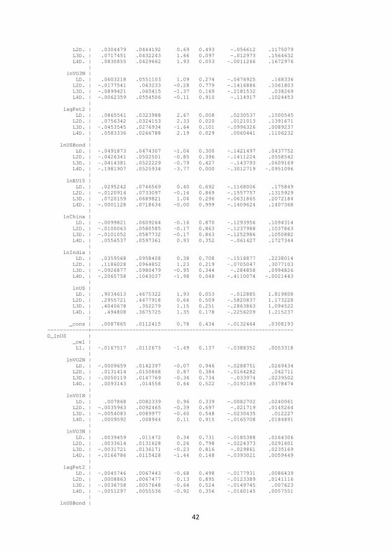
42
L2D. | .0304479 .0444192 0.69 0.493 -.056612 .1175079 L3D. | .0717451 .0432243 1.66 0.097 -.012973 .1564632 L4D. | .0830855 .0429662 1.93 0.053 -.0011266 .1672976 | lnVO3N | LD. | .0603218 .0551103 1.09 0.274 -.0476925 .168336 L2D. | -.0177541 .063233 -0.28 0.779 -.1416886 .1061803 L3D. | -.0899421 .065415 -1.37 0.169 -.2181532 .038269 L4D. | -.0062359 .0554506 -0.11 0.910 -.114917 .1024453 | lagPet2 | LD. | .0865541 .0323988 2.67 0.008 .0230537 .1500545 L2D. | .0756342 .0324153 2.33 0.020 .0121013 .1391671 L3D. | -.0453545 .0276934 -1.64 0.101 -.0996326 .0089237 L4D. | .0583336 .0266788 2.19 0.029 .0060441 .1106232 | lnUSBond | LD. | -.0491873 .0474307 -1.04 0.300 -.1421497 .0437752 L2D. | -.0426341 .0502501 -0.85 0.396 -.1411224 .0558542 L3D. | -.0414381 .0522229 -0.79 0.427 -.143793 .0609169 L4D. | -.1981907 .0525934 -3.77 0.000 -.3012719 -.0951096 | lnEU15 | LD. | .0295242 .0746569 0.40 0.692 -.1168006 .175849 L2D. | -.0120914 .0733097 -0.16 0.869 -.1557757 .1315929 L3D. | .0720159 .0689821 1.04 0.296 -.0631865 .2072184 L4D. | -.0001128 .0718634 -0.00 0.999 -.1409624 .1407368 | lnChina | LD. | -.0099821 .0609264 -0.16 0.870 -.1293956 .1094314 L2D. | -.0100063 .0580585 -0.17 0.863 -.1237988 .1037863 L3D. | -.0101052 .0587732 -0.17 0.863 -.1252986 .1050882 L4D. | .0556537 .0597361 0.93 0.352 -.061427 .1727344 | lnIndia | LD. | .0359568 .0958408 0.38 0.708 -.1518877 .2238014 L2D. | .1186028 .0964852 1.23 0.219 -.0705047 .3077103 L3D. | -.0926877 .0980479 -0.95 0.344 -.284858 .0994826 L4D. | -.2065758 .1043037 -1.98 0.048 -.4110074 -.0021443 | lnUS | LD. | .9034613 .4675322 1.93 0.053 -.012885 1.819808 L2D. | .2955721 .4477918 0.66 0.509 -.5820837 1.173228 L3D. | .4040678 .352279 1.15 0.251 -.2863863 1.094522 L4D. | .494808 .3675725 1.35 0.178 -.2256209 1.215237 | _cons | .0087865 .0112415 0.78 0.434 -.0132464 .0308193 -------------+---------------------------------------------------------------- D_lnUS | _ce1 | L1. | -.0167517 .0112673 -1.49 0.137 -.0388352 .0053318 | lnVO2N | LD. | -.0009659 .0142397 -0.07 0.946 -.0288751 .0269434 L2D. | .0131414 .0150868 0.87 0.384 -.0164282 .042711 L3D. | -.0050119 .0147769 -0.34 0.734 -.033974 .0239502 L4D. | .0093143 .014558 0.64 0.522 -.0192189 .0378474 | lnVO1N | LD. | .007868 .0082339 0.96 0.339 -.0082702 .0240061 L2D. | -.0035963 .0092465 -0.39 0.697 -.021719 .0145264 L3D. | -.0054083 .0089977 -0.60 0.548 -.0230435 .012227 L4D. | .0009592 .008944 0.11 0.915 -.0165708 .0184891 | lnVO3N | LD. | .0039459 .011472 0.34 0.731 -.0185388 .0264306 L2D. | .0033614 .0131628 0.26 0.798 -.0224373 .0291601 L3D. | -.0031721 .0136171 -0.23 0.816 -.029861 .0235169 L4D. | -.0166786 .0115428 -1.44 0.148 -.0393021 .0059449 | lagPet2 | LD. | -.0045746 .0067443 -0.68 0.498 -.0177931 .0086439 L2D. | .0008863 .0067477 0.13 0.895 -.0123389 .0141116 L3D. | -.0036758 .0057648 -0.64 0.524 -.0149745 .007623 L4D. | -.0051297 .0055536 -0.92 0.356 -.0160145 .0057551 | lnUSBond |

43
LD. | -.001275 .0098734 -0.13 0.897 -.0206264 .0180765 L2D. | .0004553 .0104603 0.04 0.965 -.0200464 .020957 L3D. | .0124128 .0108709 1.14 0.254 -.0088938 .0337194 L4D. | -.0192268 .010948 -1.76 0.079 -.0406846 .0022309 | lnEU15 | LD. | -.0261315 .0155409 -1.68 0.093 -.0565911 .004328 L2D. | .0019925 .0152604 0.13 0.896 -.0279174 .0319024 L3D. | -.0025439 .0143596 -0.18 0.859 -.0306881 .0256004 L4D. | .0019846 .0149594 0.13 0.894 -.0273352 .0313044 | lnChina | LD. | .0245317 .0126827 1.93 0.053 -.0003259 .0493893 L2D. | .0126417 .0120857 1.05 0.296 -.0110458 .0363292 L3D. | .0033561 .0122345 0.27 0.784 -.020623 .0273352 L4D. | -.0353102 .0124349 -2.84 0.005 -.0596822 -.0109382 | lnIndia | LD. | .0060974 .0199506 0.31 0.760 -.0330051 .0451998 L2D. | .0179104 .0200847 0.89 0.373 -.021455 .0572758 L3D. | .0192768 .02041 0.94 0.345 -.0207262 .0592797 L4D. | -.0140332 .0217123 -0.65 0.518 -.0565885 .0285221 | lnUS | LD. | .2701406 .0973234 2.78 0.006 .0793903 .4608909 L2D. | -.0825483 .0932141 -0.89 0.376 -.2652446 .100148 L3D. | -.1090907 .0733318 -1.49 0.137 -.2528183 .034637 L4D. | .4127324 .0765154 5.39 0.000 .262765 .5626997 | _cons | .0040883 .0023401 1.75 0.081 -.0004981 .0086748 ------------------------------------------------------------------------------ Cointegrating equations Equation Parms chi2 P>chi2 ------------------------------------------- _ce1 8 1630.66 0.0000 ------------------------------------------- Identification: beta is exactly identified Johansen normalization restriction imposed ------------------------------------------------------------------------------ beta | Coef. Std. Err. z P>|z| [95% Conf. Interval] -------------+---------------------------------------------------------------- _ce1 | lnVO2N | 1 . . . . . lnVO1N | -.6277883 .0670446 -9.36 0.000 -.7591933 -.4963833 lnVO3N | -.3062016 .0903848 -3.39 0.001 -.4833526 -.1290506 lagPet2 | -.1378976 .0486884 -2.83 0.005 -.2333251 -.04247 lnUSBond | .5049705 .0827258 6.10 0.000 .3428309 .6671101 lnEU15 | -.1546554 .0710475 -2.18 0.029 -.2939059 -.0154048 lnChina | .5445253 .1057757 5.15 0.000 .3372087 .7518419 lnIndia | -.3831463 .1153817 -3.32 0.001 -.6092903 -.1570024 lnUS | .1379354 .1224332 1.13 0.260 -.1020293 .3779001 _cons | -1.836384 . . . . . ------------------------------------------------------------------------------

44
Editor, UWA Economics Discussion Papers: Sam Hak Kan Tang University of Western Australia 35 Sterling Hwy Crawley WA 6009 Australia Email: [email protected] The Economics Discussion Papers are available at: 1980 – 2002: http://ecompapers.biz.uwa.edu.au/paper/PDF%20of%20Discussion%20Papers/ Since 2001: http://ideas.repec.org/s/uwa/wpaper1.html Since 2004: http://www.business.uwa.edu.au/school/disciplines/economics
ECONOMICS DISCUSSION PAPERS 2015
DP NUMBER
AUTHORS TITLE
15.01 Robertson, P.E. and Robitaille, M.C. THE GRAVITY OF RESOURCES AND THE TYRANNY OF DISTANCE
15.02 Tyers, R. FINANCIAL INTEGRATION AND CHINA’S GLOBAL IMPACT
15.03 Clements, K.W. and Si, J. MORE ON THE PRICE-RESPONSIVENESS OF FOOD CONSUMPTION
15.04 Tang, S.H.K. PARENTS, MIGRANT DOMESTIC WORKERS, AND CHILDREN’S SPEAKING OF A SECOND LANGUAGE: EVIDENCE FROM HONG KONG
15.05 Tyers, R. CHINA AND GLOBAL MACROECONOMIC INTERDEPENDENCE
15.06 Fan, J., Wu, Y., Guo, X., Zhao, D. and Marinova, D.
REGIONAL DISPARITY OF EMBEDDED CARBON FOOTPRINT AND ITS SOURCES IN CHINA: A CONSUMPTION PERSPECTIVE
15.07 Fan, J., Wang, S., Wu, Y., Li, J. and Zhao, D.
BUFFER EFFECT AND PRICE EFFECT OF A PERSONAL CARBON TRADING SCHEME
15.08 Neill, K. WESTERN AUSTRALIA’S DOMESTIC GAS RESERVATION POLICY THE ELEMENTAL ECONOMICS
15.09 Collins, J., Baer, B. and Weber, E.J. THE EVOLUTIONARY FOUNDATIONS OF ECONOMICS
15.10 Siddique, A., Selvanathan, E. A. and Selvanathan, S.
THE IMPACT OF EXTERNAL DEBT ON ECONOMIC GROWTH: EMPIRICAL EVIDENCE FROM HIGHLY INDEBTED POOR COUNTRIES
15.11 Wu, Y. LOCAL GOVERNMENT DEBT AND ECONOMIC GROWTH IN CHINA
15.12 Tyers, R. and Bain, I. THE GLOBAL ECONOMIC IMPLICATIONS OF FREER SKILLED MIGRATION
15.13 Chen, A. and Groenewold, N. AN INCREASE IN THE RETIREMENT AGE IN CHINA: THE REGIONAL ECONOMIC EFFECTS
15.14 Knight, K. PIGOU, A LOYAL MARSHALLIAN?

45
15.15 Kristoffersen, I. THE AGE-HAPPINESS PUZZLE: THE ROLE OF ECONOMIC CIRCUMSTANCES AND FINANCIAL SATISFACTION
15.16 Azwar, P. and Tyers, R. INDONESIAN MACRO POLICY THROUGH TWO CRISES
15.17 Asano, A. and Tyers, R. THIRD ARROW REFORMS AND JAPAN’S ECONOMIC PERFORMANCE
15.18 Arthmar, R. and McLure, M. ON BRITAIN’S RETURN TO THE GOLD STANDARD: WAS THERE A ‘PIGOU-MCKENNA SCHOOL’?
15.19 Fan, J., Li, Y., Wu, Y., Wang, S., and Zhao, D.
ALLOWANCE TRADING AND ENERGY CONSUMPTION UNDER A PERSONAL CARBON TRADING SCHEME: A DYNAMIC PROGRAMMING APPROACH
15.20 Shehabi, M. AN EXTRAORDINARY RECOVERY: KUWAIT FOLLOWING THE GULF WAR
15.21 Siddique, A., Sen, R., and Srivastava, S.
AUSTRALIA-THAILAND TRADE: AN ANALYSIS OF COMPETITIVENESS AND THE EFFECTS OF THE BILATERAL FTA
15.22 Tyers, R. SLOWER GROWTH AND VULNERABILITY TO RECESSION: UPDATING CHINA’S GLOBAL IMPACT
15.23 Arthmar, R. and McLure, M. PIGOU ON WAR FINANCE AND STATE ACTION
15.24 Wu, Y. CHINA'S CAPITAL STOCK SERIES BY REGION AND SECTOR
15.25 Clements, K. and Si, J. ENGEL'S LAW, DIET DIVERSITY AND THE QUALITY OF FOOD CONSUMPTION
15.26 Chen, S. SHIFTS OF DISTORTION AND CORRUPTION OVER LOCAL POLITICAL CYCLES IN CHINA
15.27 Chen, S. THE EFFECT OF A FISCAL SQUEEZE ON TAX NFORCEMENT: EVIDENCE FROM A NATURAL EXPERIMENT IN CHINA
15.28 Jetter, M. BLOWING THINGS UP: THE EFFECT OF MEDIA ATTENTION ON TERRORISM
15.29 Tang, S. MEDIUM-TERM MACROECONOMIC VOLATILITY AND ECONOMIC DEVELOPMENT: A NEW TECHNIQUE
15.30 Alim, A., Hartley, P. and Lan, Y. ASIAN SPOT PRICES FOR LNG OTHER ENERGY COMMODITIES
15.31 Gannon, B., Harris, D., Harris, M., Magnusson, L., Hollingsworth, B., Inder, B., Maitra, P, and Munford, L.
NEW APPROACHES TO ESTIMATING THE CHILD HEALTH-PARENTAL INCOME RELATIONSHIP
15.32 Czaika, M. and Parsons, C. THE GRAVITY OF HIGH SKILLED MIGRATION POLICIES
15.33 Parsons, C., Rojon, S., Samanani, F, and Wettach, L.
CONCEPTUALISING INTERNATIONAL HIGH-SKILLED MIGRATION
15.34 Chen, S. VAT RATE DISPERSION AND TFP LOSS IN CHINA’S MANUFACTURING SECTOR
15.35 Tait, L., Siddique, A. and Chatterjee, I. FOREIGN AID AND ECONOMIC GROWTH IN SUB-SAHARAN AFRICA

46
ECONOMICS DISCUSSION PAPERS 2016
DP NUMBER
AUTHORS TITLE
16.01 Xu, R., Wu, Y. and Luan, J. ANALYSIS OF FARMERS’ WILLINGNESS TO ADOPT GENETICALLY MODIFIED INSECT-RESISTANT RICE IN CHINA
16.02 Lia, Y., Fan, J., Zhao, D., Wu, Y. and Li, J.
TIERED GASOLINE PRICING: A PERSONAL CARBON TRADING PERSPECTIVE
16.03 Clements, K.W., Lan, Y. and Si, J. UNCERTAINTY IN CURRENCY MISPRICING
16.04 Parsons, C. and Vézina, P.L. MIGRANT NETWORKS AND TRADE:THE VIETNAMESE BOAT PEOPLE AS A NATURAL EXPERIMENT
16.05 Chang, S., Connelly, R. and Ma, P.
WHAT WILL YOU DO IF I SAY ‘I DO’?: THE EFFECT OF THE SEX RATIO ON TIME USE WITHIN TAIWANESE MARRIED COUPLES
16.06 Yu, F. and Wu, Y. BIASES IN PATENT EXAMINATION AND FIRMS’ RESPONSES: EVIDENCE FROM THE PHARMACEUTICAL INDUSTRY
16.07 Fan, J., Li, J., Wu, Y., Wang, S. and Zhao, D.
THE EFFECTS OF ALLOWANCE PRICE ON ENERGY DEMAND UNDER A PERSONAL CARBON TRADING SCHEME
16.08 Golley, J., Tyers, R. and Zhou, Y. CONTRACTIONS IN CHINESE FERTILITY AND SAVINGS: LONG RUN DOMESTIC AND GLOBAL IMPLICATIONS
16.09 McGrath, G. and Neill, K. FOREIGN AND DOMESTIC OWNERSHIP IN WESTERN AUSTRALIA’S GAS MARKET
16.10 Clements, K.W. and Si, J. SIMPLIFYING THE BIG MAC INDEX
16.11 Priyati, R.Y. and Tyers, R. PRICE RELATIONSHIPS IN VEGETABLE OIL AND ENERGY MARKETS
16.12 Wu, J., Wu, Y. and Wang, B. THE GREENNESS OF CHINESE CITIES: CARBON DIOXIDE EMISSION AND ITS DETERMINANTS
16.13 Arslan, C., Dumont, J.C., Kone, Z., Özden, Ç., Parsons, C. and Xenogiani, T.
INTERNATIONAL MIGRATION TO THE OECD IN THE TWENTY-FIRST CENTURY
16.14 Tomioka, K. and Tyers, R. HAS FOREIGN GROWTH CONTRIBUTED TO STAGNATION AND INEQUALITY IN JAPAN?
16.15 Donovan, J. and Hartley, P. RIDING THE IRON ORE CYCLE: ACTIONS OF AUSTRALIA’S MAJOR PRODUCERS