Economics 250aLocal Labor Markets

Some key referencesJennifer Roback. (1982) "Wages, Rents and the Quality of Life". JPE

90(6): 1257-1278.Enrico Moretti (2010) "Local Labor Markets". In O. Ashenfelter and D.

Card, Handbook of Labor Economics Volume 4.Pat Kline and Enrico Moretti (2013). "People, Places and Public Policy:

Some Welfare Economics of Local Economic Development Programs." NBER#19659, November 2013.Rebecca Diamond (2013) "The Determinants and Welfare Implications of

US Workers’Diverging Location Choices by Skill: 1980-2000. Unpublishedpaper.Suphanit Piyapromdee (2013). "The Impact of Immigration on Wages, In-

ternal Migration, and Welfare". University of Wisconsin Unpublished paper.Available at https://mywebspace.wisc.edu/piyapromdee/web/David Card (2001) "Immigrant Inflows, Native Outflows, and the Local Mar-

ket Impacts of Higher Immigration." JOLE 19(1).David Autor, David Dorn and Gordon Hanson (2013) "The China Syndrome:

Local Labor Market Effects of Import Competition in the United States." AER103(6).

OverviewAn area of increasing recent interest for labor economists is the study of

local labor markets. From the labor perspective, it is important to understandhow local labor supply shocks and labor demand shocks affect:- local wages, employment, unemployment- geographic mobility of workers (and firms)There is also interest in how "local policies" (local taxes, special programs

to encourage local growth) affect the local market. A key conceptual questionis how the local market equilibrium is linked to the equilibrium in other localmarkets. Different papers take different stands on this. The benchmark casewe will discuss to start this lecture assumes that workers are perfectly (andinstantaneously) mobile across areas. This imposes a very strict "constantutility" constraint on workers in every location. Recent work takes away thisassumption and tries to replace it with more reasonable assumptions aboutimperfectly elastic external supplies to each location.A related conceptual question is how sector-specific sub-markets within each

location are connected. Again, the benchmark case assumes that workers areperfectly (and instantaneously) mobile across sectors, so there is only a singlewage for each type of labor in each location. This is the same assumptionused in simple trade models. This assumption means that all workers of a givenskill type in a given location are equally affected by sectoral shocks that hit thelocation.

1

Local shocks:- on the supply side: immigration flows create location-specific shocks. Stud-

ies include Card (2001), Piyapromdee (2013). These shocks help identify theparameters of the local labor demand function. There is still substantial con-troversy over how the local demand function should be conceptualized.- on the demand side: product demand shocks create differential shocks on

net labor demand in different cities The classic "Bartik" demand shock variableis a weighted average of economy-wide employment shifts, where the weightsreflect the relative fraction of local employment in each of the sectors. Mostrecently, Autor et al (2013) have examined the effects of trade-based productdemand shocks. Local demand shocks help identify the parameters of thelocal labor supply function (broadly defined). As on the demand side, there issubstantial controversy over how to model local supply.

Equilibrating forces:There are 3 main equilibrating forces in local labor markets:- external demand for locally produced goods/services. In the classic HO

models of trade, external demand for each sector is infinitely elastic and localsupply shocks can be absorbed by sectoral expansion (subject to a diversificationconstraint). Other models allow some elasticity in external demand (Altonji-Card, 1991) or completely ignore the issue- mobility. Workers (and firms) can potentially move.- land prices. Land prices reflect the net "value" of being in a given location.

If a given location is highly productive for some external reason, land prices willcapitalize this extra productivity.

Other factors:The literature also looks at 2 other broad issues- endogenous aggregation effects. Size and composition of the workforce may

affect productivity of firms- local policies - payroll taxes, sales taxes, land restrictions, development

subsidies

Some key facts (from Moretti’s Handbook chapter)1. average wages vary a lot across cities (Tables 1 and 2), with somewhat

larger variation in wages of college educated workers

HS CollegeSan Jose $19.70 $38.50Abilene TX $11.90 $19.702. real wages, adjusting for a simple index of local housing costs, are less

variable across cities. Moreover, college grads are increasingly likely to live inhigh-cost cities, suggesting that some of the rise in average wages of collegegraduates is a (rising) compensating differential3. different counties appear to have substantially different TFP (figure 5)

2

4. firms in similar manufacturing industries tend to be geographically clus-tered, suggesting the presence of local "natural advantages", or productivityspillovers, or some other form of agglomeration economy

The Roback ModelThe basic "workhorse" model for thinking about local labor markets is pre-

sented by Roback. In the model there are homogenous workers and homogenousfirms, who have to be indifferent between alternative cities. There is a single na-tionally traded good x that is produced by firms and consumed by workers, andsells at a constant price (normalized to 1). It is assumed that each worker hasa non-labor income I that is independent of location: this can be rationalizedby assuming every worker owns a share of the land in all cities.A given city has an amenity value s: this can effect both workers’utilities

and firms’costs. In a given city the wage is w and the rental rate on a unitof land is r. (For simplicity we ignore capital).1 The number of workers wholive in a city is N : each has utility function u(x, lc, s) where x is individualconsumption, and lc is the number of units of land consumed by a worker. Aworker’s indirect utility from living in a city with amenties s, wage w and landuse price r is:

V (w, r, s) = maxx,lc

u(x, lc, s) s.t. x+ rlc − w − I = 0

Letting λ = λ(w, r, s) represent the marginal utility of a dollar of income, noticethat

Vw = λ > 0

Vr = −λlc < 0

implying thatVr = −lc(w, r, s)Vw,

which is a variant of Roy’s identify. On the firm side, each firm has CRS withunit cost function:

c(w, r, s)

Assuming total output of all firms in the city is X, total amount of land usedby firms is Lp, and total employment is N , we have:

cw = N/X > 0

cr = Lp/X > 0.

1This can be justified as follows. Assume the production function is X = g(N,L)1−θKθ,where X,N,L,K are output, labor, land, and capital, and g(N,L) is homogeneous of degree1. If capital is available at a rental rate q then setting the marginal product of capitalequal to q leads to: g(N,L)1−θ = (q/θ)K1−θ. Substituting into the production functionwe get K = (θ/q)X. Then using this fact we can rewrite the production function as X =

g(N,L)θθ/(1−θ)q−θ/(1−θ),

3

Finally, there is a total land constraint:

Lp +Nlc = L.

The indifference conditions for firms and workers across cities with differentlevels of s and endogenously varying wage and rents w(s) and r(s) respectively,are:

c(w(s), r(s), s) = 1 (1)

V (w(s), r(s), s) = V 0. (2)

Differentiating w.r.t. s we have[cw crVw Vr

] [w′(s)r′(s)

]=

[−cs−Vs

]and using the usual rules:

w′(s) =Vrcs − crVs

∆

r′(s) =Vscw − csVw

∆∆ = crVw − cwVr.

Note that we can re-write

∆ = crVw − cwVr = λLp/X + λlcN/X

= λ(Lp + lcN)/X = λL/X.

As shown in Figures 1-3 there are several special cases of interest. Case1 (Figure 1) is when cs = 0 (ie., the amenity is only valued by consumers).Clearly in this case higher s is associated with higher rents and lower wages.The split between rents and wages is determined by the slope of relation betweenw and r implied by (1). Case 2 (Figure 2) is when Vs = 0 (i.e. the amenityhas only a productivity effect). In this case a higher value of s leads to higherrents and higher wages, with the split detemined by the slope of the relationbetween w and r implied by (2). A third important benchmark (Figure 3) iswhen firms use no land and the amenity is non-productive. In this case equation(1) becomes c(w(s)) = 1, which means that the wage has to be the same in alllocations. Setting cr = cs = 0:

w′(s) = 0

r′(s) =Vscw−Vrcw

=1

lcVsVw

.

This implies that the rise in the total cost of land for a given person who livesin a city with a higher value of s is:

lcr′(s) =VsVw

.

4

The right hand side is the marginal willingness to pay for a change in s, so whencr = cs = 0, the marginal value of a change in the amenity is "fully capitalized"in rents.How do we infer the value of amenities in the more general case? Let

Ω(s) = V (w(s), r(s), s)

represent the total utility of living in city s, taking account of the endogenousadjustment of w(s) and r(s). If all cities have the same utility then

Ω′(s) = Vww′(s) + Vrr

′(s) + Vs.

Re-organizing, and using the fact that Vr = −lcVw, we get:

Vs = −Vww′(s) + lcVwr′(s)

→ VsVw

= lcr′(s)− w′(s). (3)

So the willingness to pay for the amenity can be obtained by looking at thecombination of the extra land cost for consumers and the reduced wages in ahigher-amenity city.Some more insight can be obtained by looking at the firm side. Assuming

that:c(w(s), r(s), s) = 1

across different cities, then it must be true that

cww′(s) + crr

′(s) + cs = 0

Let’s consider the case where cs = 0. In this case,

w′(s) =−crcw

r′(s)

= −Lp

Nr′(s)

So summing the willingness to pay of the N people in a given city we get

NVsVw

= Nlcr′(s) + Lpr′(s) = Lr′(s).

In the case where firms use land but cs = 0 we can get the aggregate value ofthe w.t.p. for the amenity by looking at how the total value of all land used inthe city changes as we change s.Finally let’s consider the general case where cs 6= 0. In this case the change

in sum of consumer welfare and firm profits associated with a marginal changein s is the sum of aggregate consumer w.t.p and the cost-induced savings:

dSV = NVsVw−Xcs = N(lcr′(s)− w′(s)) +X(cww

′(s) + crr′(s))

= Nlcr′(s) + Lpr′(s) = Lr′(s).

5

So the total change in social value is just the change in the value of all land.Notice that this case encompasses all the previous special cases.In her (very simple) empirical work, Roback estimated the effects of certain

amentities (Zc) on wages and residential rents. She estimated models of theform:

logwic = xiβ + γwZc + eic

log rc = γrZc + κc

The marginal value of a small change in amenity z is

VsVw

= lcr′(z)− w′(z)

= w[lcr

w

r′(z)

r− w′(z)

w]

= w[θγr − γw]

where θ = lcrw is the share of residential land rent in income. Roback estimated

this to be relatively small (3.5% on average): she estimated that mortgage costsrepresent ∼18% of income and land represents ∼20% of the value of a typicalresidential property. (These numbers are small by today’s standards). Shethen sums the marginal values of a set of 10 or so amenities (including localcrime rates, the unemployment rate, a measure of air pollution and measures ofweather), and assigns valuations to different cities.Roback also presents an extended model that has influenced subsequent an-

alysts (e.g., David Albouy, "The Unequal Geographic Burden of Federal Taxa-tion", JPE, August 2009). This model introduces a single non-traded local good”y” that is produced using land and local labor, and sells for a city-specific pricep. Think of the local good as a composite of housing services and other non-housing services (restaurants, etc). Now the indirect utility function is

V (w, p, s) = maxx,y

u(x, y, s) s.t. x+ py = w + I

and there are 2 unit cost functions: one for the tradeable good (as before)

c(w, r, s) = 1

and another for the local good:

g(w, r, s) = p.

Now there are 3 endogenous variables (w, r, p), but the basic ideas in the pre-ceding analysis are still present. An interesting application of this frameworkis to an amenity s that raises the cost of the local good, but has no inherentvalue for consumers or productivity effects on the traded sector. This could beineffi ciency in the local construction sector, for example.

Allowing for Heterogeneity in Tastes

6

A major limitation of the Roback model is that all workers are indifferentto living in different cities. This is obviously false: a majority of people live inthe state where they were born. Indeed, Severnini (2013) estimates that 80%of white couples live in a state where at least one of the two partners was born(though this ratio is only 33% if both have a PhD). Kline and Moretti (2013)present a very simple model based on Busso, Gregory and Kline (AER, 2013)in which people have idiosyncratic preferences for cities. They assume

uic = wc − rc +Ac − t+ eic

where wc and rc are the levels of wages and rents in city c, Ac is an amenity inthe city, t is a common (lump sum) tax, and eic is a taste factor. They assumeeic/s is EV-1, which generates a MNL model. Notice that as s → 0 peoplebecome more "attached" to specific cities, so s governs the elasticity of supplyto a given city. The linearity of preferences is restrictive but greatly simplifiesthe analysis. They add a simple traded good sector that implies

logwc = d0 + d log δc − log(1 + τ c)

where δc is a TFP shifter, τ c is a local wage tax or credit, d0 is a constant thatvaries with the cost of capital, and d is another constant (KM use Xc as thesymbol for δc). This means that the "labor demand curve" is horizontal in anycity, but shifts up or down depending on δc. They complete the model with aninverse "housing supply" function:

rc = zc(Nc)kc .

Letting vc = wc − rc +Ac − t, person i chooses city a over city b iff:

eib − eias

≤ va − vbs

soNa = NF [

va − vbs

]

where N is the total population and F is the d.f. for a logit (the difference in 2EV-1’s). Setting N = 1 and re-arranging:

sF−1(Na) = wa − wb − (ra − rb) +Aa −Ab

= ed0(δda

1 + τa− δdb

1 + τa)− (za(Na)ka − zb(1−Na)kb) +Aa −Ab

The lhs is an upward-sloping inverse-S shaped function of Na, while the rhsis a negatively sloped function, leading to K-M’s figure 1. They show how touse this simple model to discuss the effects of local tax/subsidy policies. Aninteresting extension is to the case where δc depends on the size of city c. Ifthis effect is large enough, the rhs of the above equation can become upwardsloping, leading to potential multiple equilibria (see KM figure 4).

7

Piyapromdee — Allowing for Different Skill Groups and Heterogeneity inTastesPiyapromdee is an ambitious attempt to extend the Roback type frame-

work to allow different skill groups and taste heterogeneity. She assumes thatworkers are classified in 4 ways: education level (college/HS); gender; age (2groups, young and old), and immigrant status. She assumes that each city hasa 4-level nested CES production function producing a common traded good.The parameters of this model are estimated "stepwise", as in Card-Lemieuxand Ottaviano-Peri, but using a combination of time and city-level variation(1980-1990-2000 Census plus 2007 ACS). The parameters for education, ageand immigrant status are similar to those estimated by O-P. The estimatedelasticity of substitution between men and women in the same education groupis 1.9 (standard error=0.6), which is suprisingly small.At the city level she assumes a housing supply model similar to the one in

K-M. Specifically, she assumes a housing "rental rate" in city c in year t:

Rct = it × CCct × [∑j

γhHjct +∑j

Ljct]γc

where it iis the interest rate in year t, CCct is an (unobserved) construction costfor city c in year t, Hjct is the number of high-education workers in subgroup jin city c in year t (so j runs over immigrants/natives + young/old + gender),Ljct is the number of low-ed. workers in group j, γh is a scale factor (=1.68—see footnote 36), and γc is a city-specific supply elasticity that is allowed tovary with a measure of the fraction of undevelopeable land within 50 km of thecenter of each MSA area (so this is 1/2 for a city like Miami with a center veryclose to the ocean), and with an index of local land regulations (see equation11, p. 13).The final part of the model is a MNL choice model of preferences for different

cities. The basic specification of utility is

Uict = maxQ,G

λz log(Q)+(1−λz) log(G)+ui(Nct)+σzεict s.t. PtG+RctQ = W zct

where: Q is an amount of housing (with local price Rct), G is an amount ofthe numeraire good (with national price Pt),W z

ct is the wage earned by a personin group z = z(i) (based on education, gender, age, and immigrant status),λz is a housing share parameter that varies by education level only, εict is anEV-1 error with scale σz, and ui(Nct) is a person-specific utility assigned to the"network characteristics" Nct of city c in year t — this includes the fractionsof various immigrant groups in the city in an earlier decade, which are valueddifferently by immmigrants from different source countries, as well as dummiesfor which state a city is in, which are valued differently by people who were bornin different states. Doing the maximization we get:

Uict = log(W zct/Pt)− λz log(Rct/Pt) + ui(Nct) + σzεict

= wzct − λzrct + βzXict + σzεict

8

where P. is assuming that we can write ui(Nct) = βzXict (this is my notationfor what she does). Note the functional form: indirect utility depends on logreal wage (wzct), and on the log of real housing prices (rct), but the weight onthe real housing price depends on λi. If (for example) a person spends about40% of their income on housing then we expect λi = 0.40. Re-normalizing theindirect utility by dividing by σz yields

Uict = λwz (wzct − λzrct) + λxzXict + εict

= Γzct + λxzXict + εict

where Γzct is the common value for city c in year t for all people in group z. Noticethat all the "endogeneity" problems caused by endogenous variation in wzct orrct are rolled into Γzct, while the person-specific component reflects interactionsbetween a person’s state of birth and the location of the city, or a person’scountry of birth and the shares of previous immigrants from the same countryin the city 10 years ago. This leads to a two-step "micro-BLP" approach ofestimating a MNL for location choice for person i that includes Γzct dummiesand the person-specific components, then in the second stage the parametersfor the determinants of Γzct are estimated using the estimates, Γzct.

P. estimates a model for the Γzct terms in first-differences:

∆Γzct ≡ Γzct − Γzct−10 = λwz (∆wzct − λz∆rct) + ∆amenityzct + sampling error

where∆amenityzct reflects the change in the (common) amenity value of city c topeople in group z. Since changes in amenities may be correlated with wage/rentchanges, instruments are needed. P uses "Bartik" shift-share instruments (basedon lagged industry shares in the city and national changes in employment in eachindustry), interacted with the 2 shifters of local housing elasticity (the share ofundevelopeable land, and the index of land use reguations). Note that P. callsthe Bartik shock variables "Katz Murphy" indexes (KM). (( recall that P. treatsλ′zs as known). Estimates of the key parameter λ

wz = 1/σz are reported in Table

5:High-education natives 4.0Low-education natives 3.7High-education imms 1.2Low-education imms 0.7

9

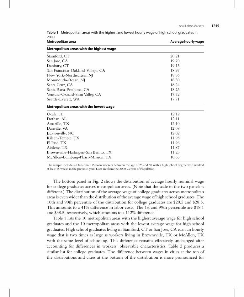
Local Labor Markets 1245

Table 1 Metropolitan areas with the highest and lowest hourly wage of high school graduates in2000.Metropolitan area Averagehourlywage

Metropolitan areas with the highest wage

Stamford, CT 20.21San Jose, CA 19.70Danbury, CT 19.13San Francisco-Oakland-Vallejo, CA 18.97New York-Northeastern NJ 18.86Monmouth-Ocean, NJ 18.30Santa Cruz, CA 18.24Santa Rosa-Petaluma, CA 18.23Ventura-Oxnard-Simi Valley, CA 17.72Seattle-Everett, WA 17.71

Metropolitan areas with the lowest wage

Ocala, FL 12.12Dothan, AL 12.11Amarillo, TX 12.10Danville, VA 12.08Jacksonville, NC 12.02Kileen-Temple, TX 11.98El Paso, TX 11.96Abilene, TX 11.87Brownsville-Harlingen-San Benito, TX 11.23McAllen-Edinburg-Pharr-Mission, TX 10.65

The sample includes all full-time US born workers between the age of 25 and 60 with a high school degree who workedat least 48 weeks in the previous year. Data are from the 2000 Census of Population.

The bottom panel in Fig. 2 shows the distribution of average hourly nominal wagefor college graduates across metropolitan areas. (Note that the scale in the two panels isdifferent.) The distribution of the average wage of college graduates across metropolitanareas is even wider than the distribution of the average wage of high school graduates. The10th and 90th percentile of the distribution for college graduates are $20.5 and $28.5.This amounts to a 41% difference in labor costs. The 1st and 99th percentile are $18.1and $38.5, respectively, which amounts to a 112% difference.

Table 1 lists the 10 metropolitan areas with the highest average wage for high schoolgraduates and the 10 metropolitan areas with the lowest average wage for high schoolgraduates. High school graduates living in Stamford, CT or San Jose, CA earn an hourlywage that is two times as large as workers living in Brownsville, TX or McAllen, TXwith the same level of schooling. This difference remains effectively unchanged afteraccounting for differences in workers’ observable characteristics. Table 2 produces asimilar list for college graduates. The difference between wages in cities at the top ofthe distributions and cities at the bottom of the distribution is more pronounced for

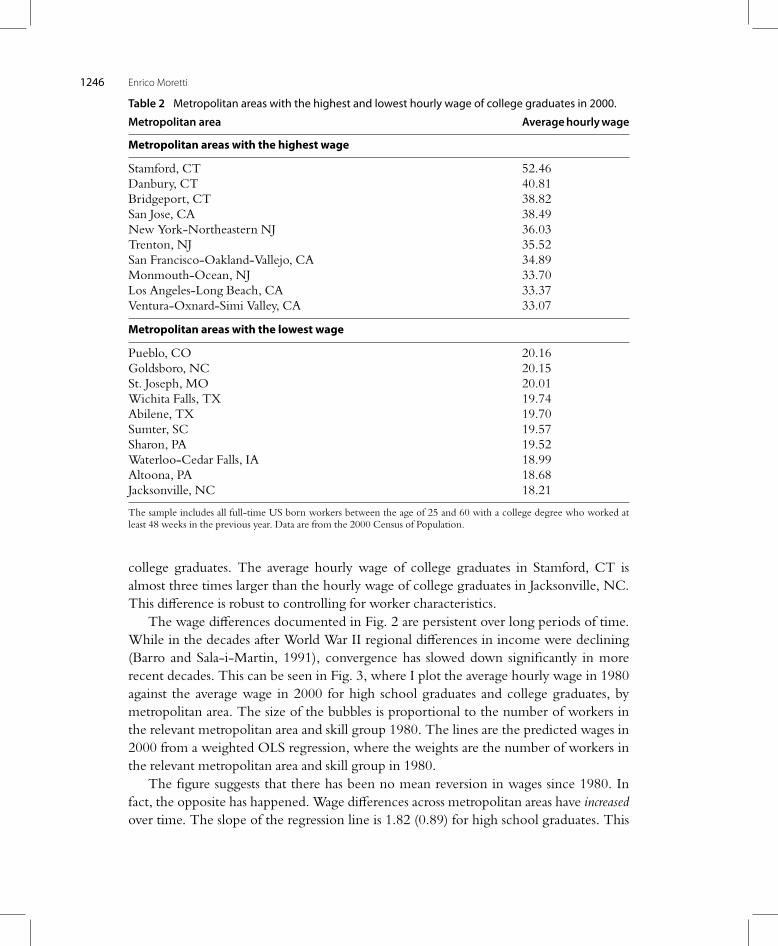
1246 Enrico Moretti

Table 2 Metropolitan areas with the highest and lowest hourly wage of college graduates in 2000.

Metropolitan area Averagehourlywage

Metropolitan areas with the highest wage

Stamford, CT 52.46Danbury, CT 40.81Bridgeport, CT 38.82San Jose, CA 38.49New York-Northeastern NJ 36.03Trenton, NJ 35.52San Francisco-Oakland-Vallejo, CA 34.89Monmouth-Ocean, NJ 33.70Los Angeles-Long Beach, CA 33.37Ventura-Oxnard-Simi Valley, CA 33.07

Metropolitan areas with the lowest wage

Pueblo, CO 20.16Goldsboro, NC 20.15St. Joseph, MO 20.01Wichita Falls, TX 19.74Abilene, TX 19.70Sumter, SC 19.57Sharon, PA 19.52Waterloo-Cedar Falls, IA 18.99Altoona, PA 18.68Jacksonville, NC 18.21

The sample includes all full-time US born workers between the age of 25 and 60 with a college degree who worked atleast 48 weeks in the previous year. Data are from the 2000 Census of Population.

college graduates. The average hourly wage of college graduates in Stamford, CT isalmost three times larger than the hourly wage of college graduates in Jacksonville, NC.

This difference is robust to controlling for worker characteristics.The wage differences documented in Fig. 2 are persistent over long periods of time.

While in the decades after World War II regional differences in income were declining(Barro and Sala-i-Martin, 1991), convergence has slowed down significantly in morerecent decades. This can be seen in Fig. 3, where I plot the average hourly wage in 1980against the average wage in 2000 for high school graduates and college graduates, bymetropolitan area. The size of the bubbles is proportional to the number of workers inthe relevant metropolitan area and skill group 1980. The lines are the predicted wages in2000 from a weighted OLS regression, where the weights are the number of workers inthe relevant metropolitan area and skill group in 1980.

The figure suggests that there has been no mean reversion in wages since 1980. Infact, the opposite has happened. Wage differences across metropolitan areas have increasedover time. The slope of the regression line is 1.82 (0.89) for high school graduates. This

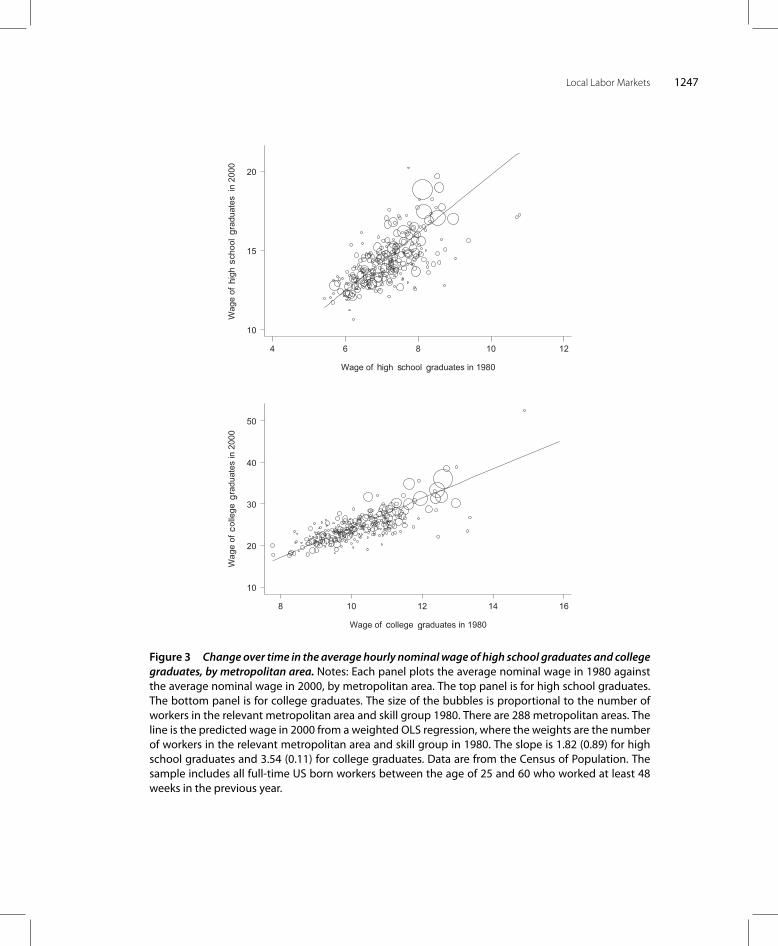
Local Labor Markets 1247

Figure 3 Change over time in the average hourly nominalwage of high school graduates and collegegraduates, by metropolitan area. Notes: Each panel plots the average nominal wage in 1980 againstthe average nominal wage in 2000, by metropolitan area. The top panel is for high school graduates.The bottom panel is for college graduates. The size of the bubbles is proportional to the number ofworkers in the relevant metropolitan area and skill group 1980. There are 288 metropolitan areas. Theline is the predicted wage in 2000 from a weighted OLS regression, where the weights are the numberof workers in the relevant metropolitan area and skill group in 1980. The slope is 1.82 (0.89) for highschool graduates and 3.54 (0.11) for college graduates. Data are from the Census of Population. Thesample includes all full-time US born workers between the age of 25 and 60 who worked at least 48weeks in the previous year.

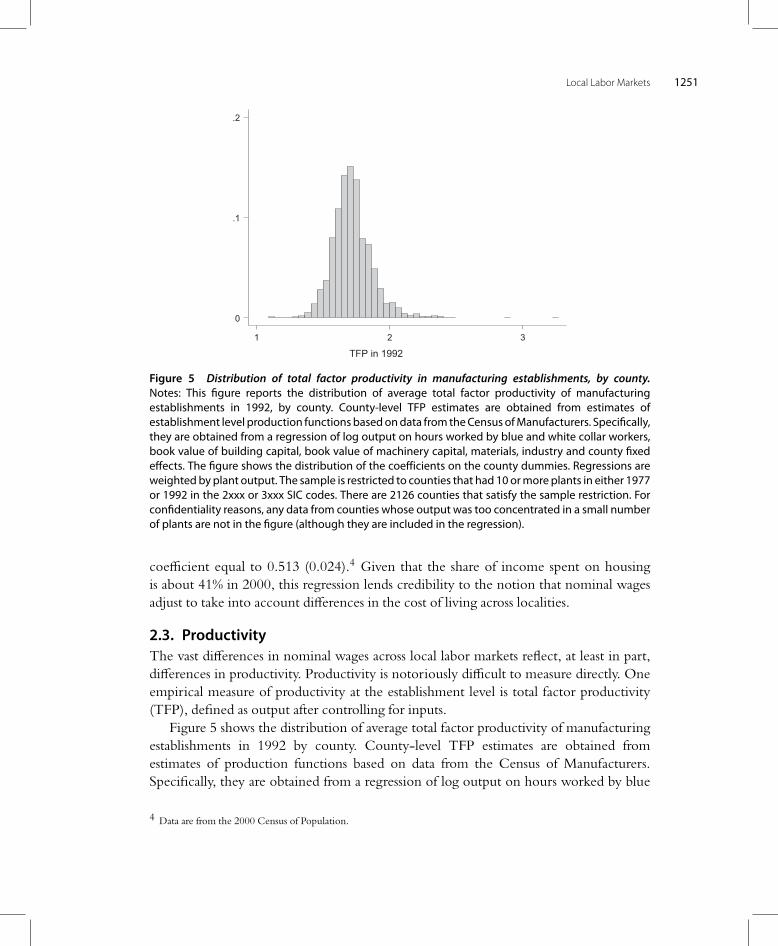
Local Labor Markets 1251

Figure 5 Distribution of total factor productivity in manufacturing establishments, by county.Notes: This figure reports the distribution of average total factor productivity of manufacturingestablishments in 1992, by county. County-level TFP estimates are obtained from estimates ofestablishment level production functionsbasedondata from theCensus ofManufacturers. Specifically,they are obtained from a regression of log output on hours worked by blue and white collar workers,book value of building capital, book value of machinery capital, materials, industry and county fixedeffects. The figure shows the distribution of the coefficients on the county dummies. Regressions areweightedbyplant output. The sample is restricted to counties that had 10 ormore plants in either 1977or 1992 in the 2xxx or 3xxx SIC codes. There are 2126 counties that satisfy the sample restriction. Forconfidentiality reasons, any data from counties whose output was too concentrated in a small numberof plants are not in the figure (although they are included in the regression).

coefficient equal to 0.513 (0.024).4 Given that the share of income spent on housingis about 41% in 2000, this regression lends credibility to the notion that nominal wagesadjust to take into account differences in the cost of living across localities.

2.3. ProductivityThe vast differences in nominal wages across local labor markets reflect, at least in part,differences in productivity. Productivity is notoriously difficult to measure directly. Oneempirical measure of productivity at the establishment level is total factor productivity(TFP), defined as output after controlling for inputs.

Figure 5 shows the distribution of average total factor productivity of manufacturingestablishments in 1992 by county. County-level TFP estimates are obtained fromestimates of production functions based on data from the Census of Manufacturers.Specifically, they are obtained from a regression of log output on hours worked by blue

4 Data are from the 2000 Census of Population.

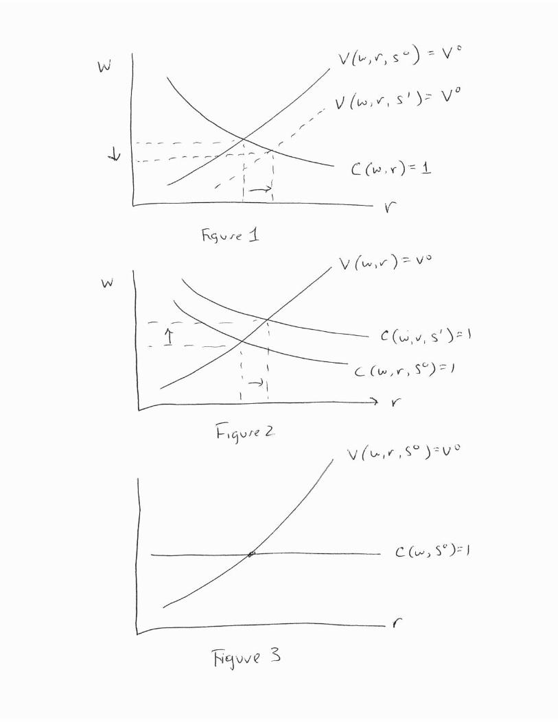
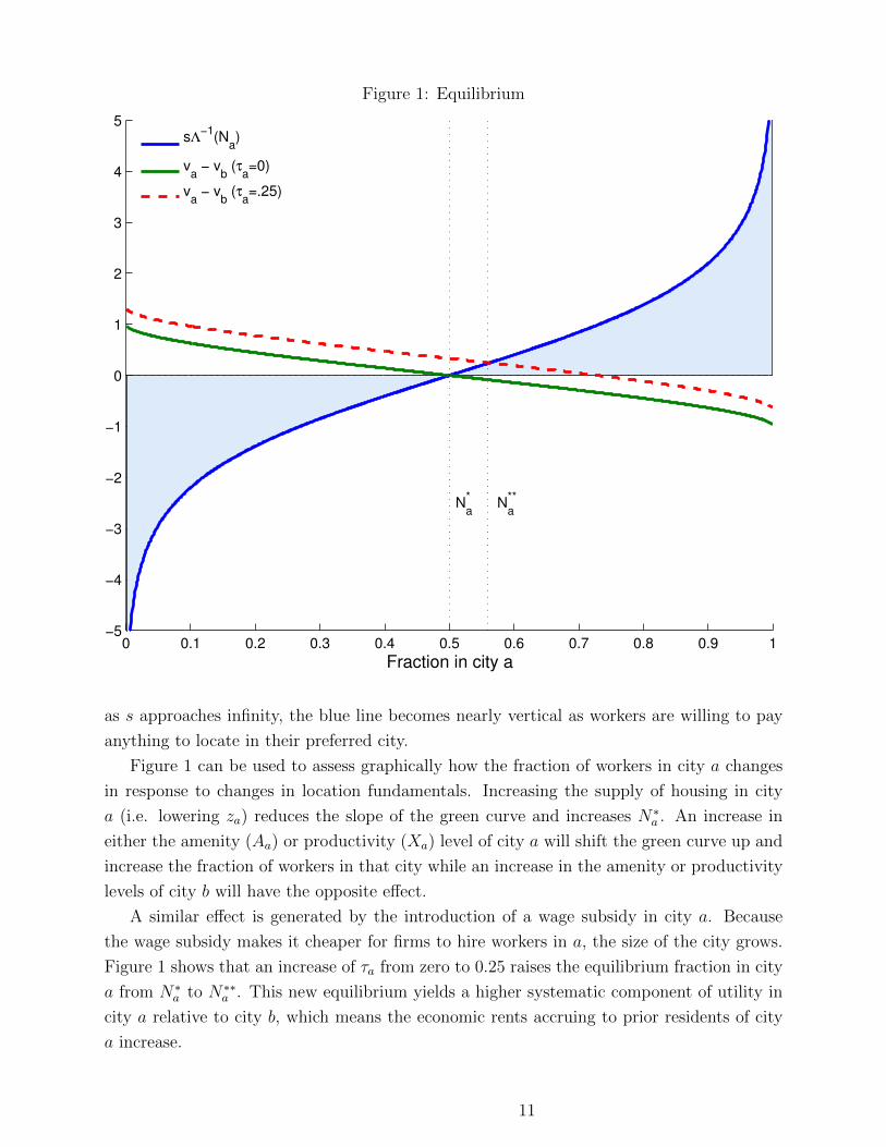
Figure 1: Equilibrium

0 0.1 0.2 0.3 0.4 0.5 0.6 0.7 0.8 0.9 1−5

−4

−3

−2

−1

0

1

2

3

4

5

Fraction in city a

sΛ

−1(N

a)

va − v

b (τ

a=0)

va − v

b (τ

a=.25)

Na

*N

a

**

as s approaches infinity, the blue line becomes nearly vertical as workers are willing to pay

anything to locate in their preferred city.

Figure 1 can be used to assess graphically how the fraction of workers in city a changes

in response to changes in location fundamentals. Increasing the supply of housing in city

a (i.e. lowering za) reduces the slope of the green curve and increases N∗a . An increase in

either the amenity (Aa) or productivity (Xa) level of city a will shift the green curve up and

increase the fraction of workers in that city while an increase in the amenity or productivity

levels of city b will have the opposite effect.

A similar effect is generated by the introduction of a wage subsidy in city a. Because

the wage subsidy makes it cheaper for firms to hire workers in a, the size of the city grows.

Figure 1 shows that an increase of τa from zero to 0.25 raises the equilibrium fraction in city

a from N∗a to N∗∗a . This new equilibrium yields a higher systematic component of utility in

city a relative to city b, which means the economic rents accruing to prior residents of city

a increase.

11

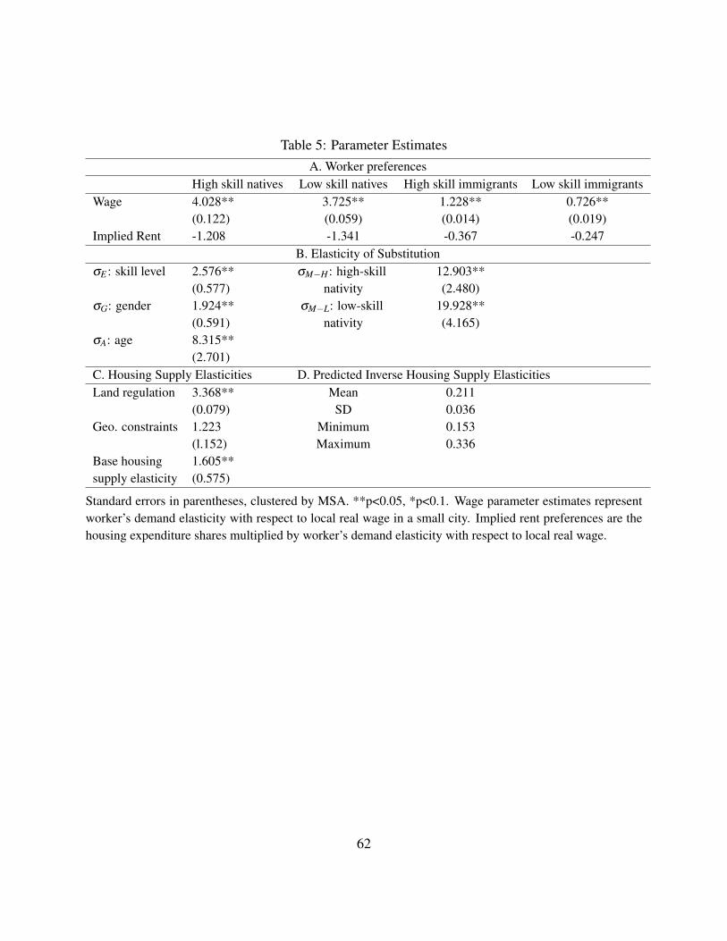
Table 5: Parameter EstimatesA. Worker preferences

High skill natives Low skill natives High skill immigrants Low skill immigrantsWage 4.028** 3.725** 1.228** 0.726**

(0.122) (0.059) (0.014) (0.019)Implied Rent -1.208 -1.341 -0.367 -0.247

B. Elasticity of SubstitutionσE : skill level 2.576** σM−H : high-skill 12.903**

(0.577) nativity (2.480)σG: gender 1.924** σM−L: low-skill 19.928**

(0.591) nativity (4.165)σA: age 8.315**

(2.701)C. Housing Supply Elasticities D. Predicted Inverse Housing Supply ElasticitiesLand regulation 3.368** Mean 0.211

(0.079) SD 0.036Geo. constraints 1.223 Minimum 0.153

(l.152) Maximum 0.336Base housing 1.605**supply elasticity (0.575)

Standard errors in parentheses, clustered by MSA. **p<0.05, *p<0.1. Wage parameter estimates representworker’s demand elasticity with respect to local real wage in a small city. Implied rent preferences are thehousing expenditure shares multiplied by worker’s demand elasticity with respect to local real wage.

62

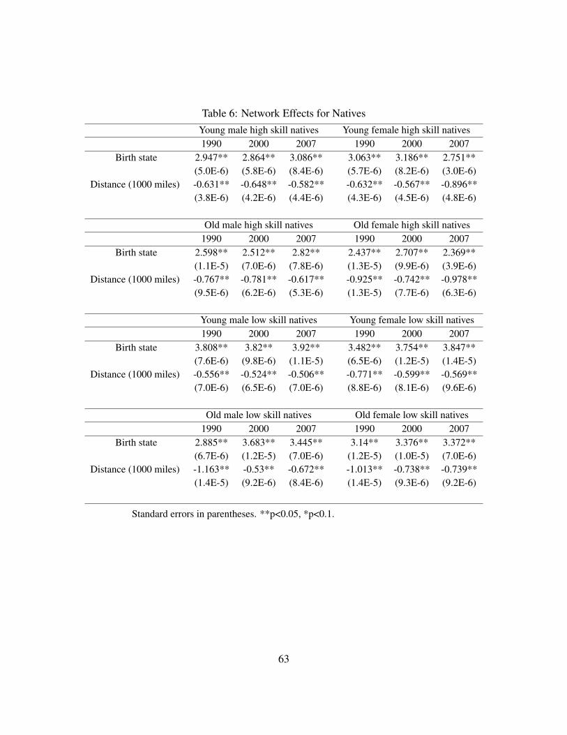
Table 6: Network Effects for NativesYoung male high skill natives Young female high skill natives1990 2000 2007 1990 2000 2007

Birth state 2.947** 2.864** 3.086** 3.063** 3.186** 2.751**(5.0E-6) (5.8E-6) (8.4E-6) (5.7E-6) (8.2E-6) (3.0E-6)

Distance (1000 miles) -0.631** -0.648** -0.582** -0.632** -0.567** -0.896**(3.8E-6) (4.2E-6) (4.4E-6) (4.3E-6) (4.5E-6) (4.8E-6)

Old male high skill natives Old female high skill natives1990 2000 2007 1990 2000 2007

Birth state 2.598** 2.512** 2.82** 2.437** 2.707** 2.369**(1.1E-5) (7.0E-6) (7.8E-6) (1.3E-5) (9.9E-6) (3.9E-6)

Distance (1000 miles) -0.767** -0.781** -0.617** -0.925** -0.742** -0.978**(9.5E-6) (6.2E-6) (5.3E-6) (1.3E-5) (7.7E-6) (6.3E-6)

Young male low skill natives Young female low skill natives1990 2000 2007 1990 2000 2007

Birth state 3.808** 3.82** 3.92** 3.482** 3.754** 3.847**(7.6E-6) (9.8E-6) (1.1E-5) (6.5E-6) (1.2E-5) (1.4E-5)

Distance (1000 miles) -0.556** -0.524** -0.506** -0.771** -0.599** -0.569**(7.0E-6) (6.5E-6) (7.0E-6) (8.8E-6) (8.1E-6) (9.6E-6)

Old male low skill natives Old female low skill natives1990 2000 2007 1990 2000 2007

Birth state 2.885** 3.683** 3.445** 3.14** 3.376** 3.372**(6.7E-6) (1.2E-5) (7.0E-6) (1.2E-5) (1.0E-5) (7.0E-6)

Distance (1000 miles) -1.163** -0.53** -0.672** -1.013** -0.738** -0.739**(1.4E-5) (9.2E-6) (8.4E-6) (1.4E-5) (9.3E-6) (9.2E-6)

Standard errors in parentheses. **p<0.05, *p<0.1.

63

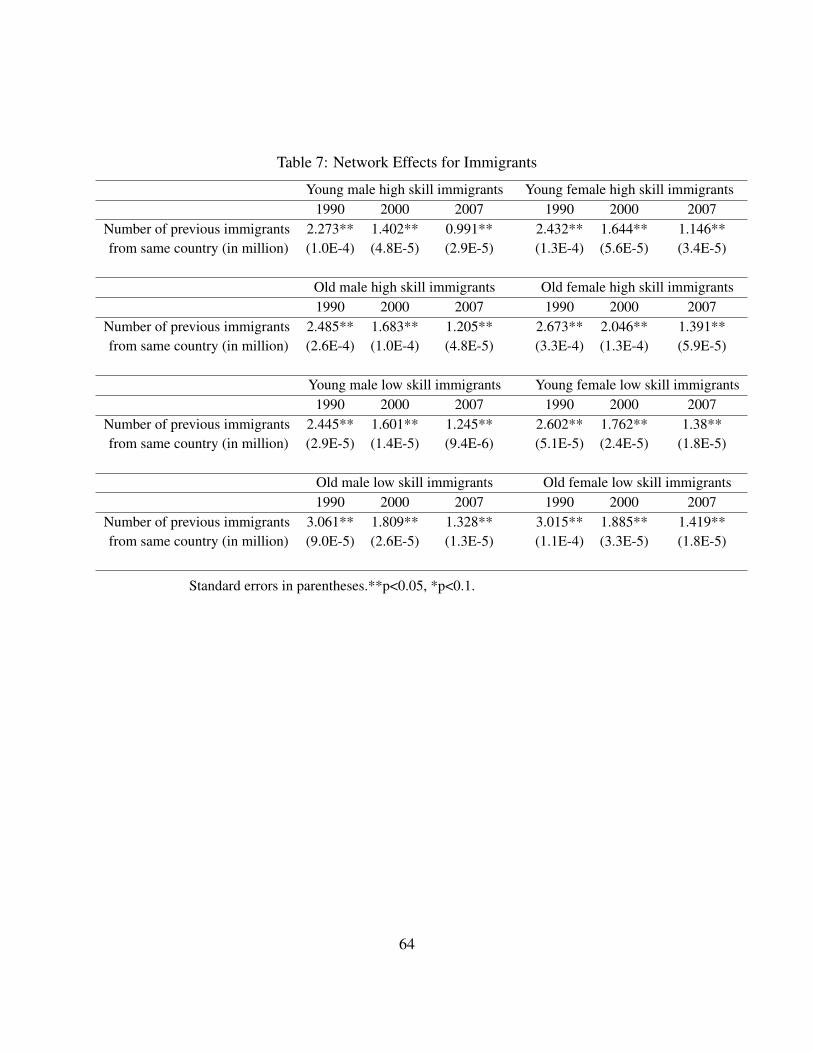
Table 7: Network Effects for Immigrants

Young male high skill immigrants Young female high skill immigrants1990 2000 2007 1990 2000 2007

Number of previous immigrants 2.273** 1.402** 0.991** 2.432** 1.644** 1.146**from same country (in million) (1.0E-4) (4.8E-5) (2.9E-5) (1.3E-4) (5.6E-5) (3.4E-5)

Old male high skill immigrants Old female high skill immigrants1990 2000 2007 1990 2000 2007

Number of previous immigrants 2.485** 1.683** 1.205** 2.673** 2.046** 1.391**from same country (in million) (2.6E-4) (1.0E-4) (4.8E-5) (3.3E-4) (1.3E-4) (5.9E-5)

Young male low skill immigrants Young female low skill immigrants1990 2000 2007 1990 2000 2007

Number of previous immigrants 2.445** 1.601** 1.245** 2.602** 1.762** 1.38**from same country (in million) (2.9E-5) (1.4E-5) (9.4E-6) (5.1E-5) (2.4E-5) (1.8E-5)

Old male low skill immigrants Old female low skill immigrants1990 2000 2007 1990 2000 2007

Number of previous immigrants 3.061** 1.809** 1.328** 3.015** 1.885** 1.419**from same country (in million) (9.0E-5) (2.6E-5) (1.3E-5) (1.1E-4) (3.3E-5) (1.8E-5)

Standard errors in parentheses.**p<0.05, *p<0.1.

64