Economic Valuation of Product Features

⇤

Greg M. Allenby

Fisher College of Business

Ohio State University

Jeff Brazell

The Modellers

John R. Howell

Smeal College of Business

Pennsylvania State University

Peter E. Rossi

Anderson School of Management

UCLA

September 2013

revised, October 2013

Abstract

We develop a market-based paradigm to value the enhancement or addition of features

to a product. We define the market value of a product or feature enhancement as the

change in the equilibrium profits that would prevail with and without the enhancement.

Conjoint data can be use to construct the demand system necessary to compute equilib-

rium prices but assumptions about competitive offerings and cost are required as well. We

contrast our approach to the frequent practice of computing what we call pseudo-WTP

(willingness to pay) and show that pseudo-WTP may greatly over-estimate the value of

a feature. We illustrate our methods using a survey of digital camera owners.

⇤Rossi would like to acknowledge the Collins Chair, Anderson School of Management, UCLA for reearchfunding. Allenby thanks the Fisher College of Business at Ohio State University for generous research support.All correspondence may be addressed to the authors at the UCLA, Anderson School of Management, 110Westwood Plaza, Los Angeles, CA 90095; or via e-mail at perossichi@gmail.com.

1

1 Introduction

Valuation of product features is a critical part of the development and marketing of products

and services. Firms are continuously involved in the improvement of existing products by

adding new features and many “new products” are essentially old products which have been

enhanced with features previously unavailable. For example, consider the smartphone cate-

gory of products. As new generations of smartphones are produced and marketed, existing

features such as screen resolution/size or cellular network speed are enhanced to new higher

levels. In addition, features are added to enhance the usability of smartphone. These new

features might include integration of social networking functions into the camera application

of the smartphone. A classic example, which was involved in litigation between Apple and

Samsung, is the use of icons with rounded edges. New and enhanced features often involve

substantial development costs and sometimes also require new components which drive up

the marginal cost of production.

The decision to develop new features is a strategic decision involving not only the cost of

adding the feature but also the possible competitive response. The development and marketing

costs of feature enhancement must be weighed against the expected increase in profits which

will accrue if the product feature is added or enhanced. Expected profits in a world with the

new feature must be compared to expected profits in a world without the feature. Computing

this change in expected profits involves predicting not only demand for the feature but also

assessing the new industry equilibrium that will prevail with a new set of products and

competitive offerings.

In a litigation context, product features are often at the core of patent disputes.1 The

practical content of both apparatus and method patents can be viewed as the enabling of

product features. The potential value of the product feature(s) enabled by patent is what

gives the patent value. That is, patents are valuable only to the extent that they enable1In this paper, we will not consider the legal questions of whether or not the patent is valid and whether or

not the defendant has infringed the patent(s) in dispute. We will focus on the economic value of the featuresenabled by the patent. The market value of the patent is determined both by the value of the features enabledas well as by the probability that the patent will be deemed to be a valid patent and the costs of defendingthe patent’s validity and enforcement.

2

product features not obtainable via other (so-called “non-infringing”) means. Valuation of

product features places a central role in damages analysis for patent disputes. Damages may

accrue to the patent holder either from royalty fees that should have been paid by the firm

accused of infringing the patent and, in some cases, because the patent holder’s existing

products suffer from lost profits from the infringing products. In either case, the valuation of

the product feature in terms of expected profits will be at the core of the damages analysis.

The hypothetical negotiation for royalties can be viewed as comprised of two parts: 1. what

is the value of the patent in terms of increases in expected profits for the licensee? and 2.

how should these expected profits be divided between the licensor and licensee. In lost profits

analysis, we must compare actual sales of the licensor’s products that practice the patent to

the sales that would have occurred in the absence of competition from the accused products

and compute profits on this change in sales. This is closely related to the problem of predicting

incremental profits from use of the patent-enabled feature.

In both commercial and litigation realms, therefore, valuation of product features is crit-

ical to decision making and damages analysis. Conjoint Analysis (see, for example, Orme

(2009) and Gustafsson, Herrmann, and Huber (2000)) is designed to measure and simulate

demand in situations where products can be assumed to be comprised of bundles of features.

While conjoint analysis has been used for many years in product design (see the classic ex-

ample in Green and Wind (1989)), the use of conjoint in patent litigation has only developed

recently. Both uses of conjoint stem from the need to predict demand in the future (after the

new product has been released) or in a counterfactual world in which the accused infringing

products are withdrawn from the market. However, the literature has struggled, thus far, to

precisely define meaning of “value” as applied to product features. The current practice is to

compute what many authors call a Willingness to Pay (hereafter, WTP) or a Willingness To

Buy (hereafter, WTB). WTP for a product feature enhancement is defined as the monetary

amount which would be sufficient to compensate a consumer for the loss of the product fea-

ture or for a reduction to the non-enhanced state. WTB is defined as the change in sales or

market share that would occur as the feature is added or enhanced. The problem with both

3

the WTP and WTB measures is that they are not equilibrium outcomes. WTP measures

only a shift in the demand curve and not what the change in equilibrium price will be as the

feature is added or enhanced. WTB holds prices fixed and does not account for the fact that

as a product becomes more valuable equilibrium prices will typically go up.

We advocate using equilibrium outcomes (both price and shares) to determine the incre-

mental economic profits that would accrue to a firm as a product is enhanced. In general,

the WTP measure will overstate the change in equilibrium price and profits and the WTB

measure will overstate the change in equilibrium market share. We illustrate this using a

conjoint survey for digital cameras and the addition of a swivel screen display as the object

of the valuation exercise. Standard WTP measures are shown to greatly overstate the value

of the product feature.

To compute equilibrium outcomes, we will have to make assumptions about cost and

the nature of competition and the set of competitive offers. Conjoint studies will have to

be designed with this in mind. In particular, greater care to include an appropriate set of

competitive brands, handle the outside option appropriately, and estimate price sensitivity

precisely must be exercised.

2 Pseudo-WTP, True WTP, and WTB

In the context of conjoint studies, feature valuation is achieved by using various measures that

relate only to the demand for the products and features and not to the supply. In particular,

it is common to produce estimates of what some call Willingness To Pay and Willingness To

Buy. Both WTP and WTB depend only on the parameters of the demand system. As such,

the WTP and WTB measure cannot be measures of the market value of a product feature

as they do not directly relate to what incremental profits a firm can earn on the basis of the

product feature. In this section, we review the WTP and WTB measures and explain the

likely biases in these measures in feature valuation. We also explain why the WTP measures

used in practice are not true WTP measures and provide the correct definition of WTP.

4

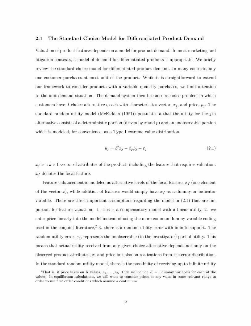
2.1 The Standard Choice Model for Differentiated Product Demand

Valuation of product features depends on a model for product demand. In most marketing and

litigation contexts, a model of demand for differentiated products is appropriate. We briefly

review the standard choice model for differentiated product demand. In many contexts, any

one customer purchases at most unit of the product. While it is straightforward to extend

our framework to consider products with a variable quantity purchases, we limit attention

to the unit demand situation. The demand system then becomes a choice problem in which

customers have J choice alternatives, each with characteristics vector, xj

, and price, pj

. The

standard random utility model (McFadden (1981)) postulates a that the utility for the jth

alternative consists of a deterministic portion (driven by x and p) and an unobservable portion

which is modeled, for convenience, as a Type I extreme value distribution.

u

j

= �

0x

j

� �

p

p

j

+ "

j

(2.1)

x

j

is a k⇥ 1 vector of attributes of the product, including the feature that requires valuation.

x

f

denotes the focal feature.

Feature enhancement is modeled as alternative levels of the focal feature, xf

(one element

of the vector x), while addition of features would simply have x

f

as a dummy or indicator

variable. There are three important assumptions regarding the model in (2.1) that are im-

portant for feature valuation: 1. this is a compensatory model with a linear utility, 2. we

enter price linearly into the model instead of using the more common dummy variable coding

used in the conjoint literature,2 3. there is a random utility error with infinite support. The

random utility error, "j

, represents the unobservable (to the investigator) part of utility. This

means that actual utility received from any given choice alternative depends not only on the

observed product attributes, x, and price but also on realizations from the error distribution.

In the standard random utility model, there is the possibility of receiving up to infinite utility2That is, if price takes on K values, p1, . . . , pK , then we include K � 1 dummy variables for each of the

values. In equilibrium calculations, we will want to consider prices at any value in some relevant range inorder to use first order conditions which assume a continuum.

5

from the choice alternative. This means that in evaluating the option to make choices from a

set of products, we must consider the contribution not only of the observed or deterministic

portion of utility but also the distribution of the utility errors. The possibilities for realization

from the error distribution provide a source of utility for each choice alternative.

To derive the standard choice model, we must calculate the probability that the jth

alternative has the maximum utility, employing the assumption that the error terms have a

specific distribution. As is well known, the utility index in (2.1) is arbitrary and is preserved

under both a location and scale shift. That is, if any number is subtracted from the utility of

all choice alternatives, then the index of the maximum remains unchanged. Another way of

saying this is that utility can only be expressed in a relative sense and that utility is not on

a ratio scale. This is also true that the index of the maximum utility is not changed if each

alternative scaled by the same positive number. In conjoint applications with dummy variable

coding the attributes (each level except one is introduced via dummy variables), there is one

level of all variables (the “default” or base level) which is assigned a utility of zero. This

means that, in conjoint designs, there is no location invariance problem. However, there is

still a scaling problem. Typically, researchers set the scale parameter of the Type I extreme

value distribution to 1. Another approach to the scaling invariance problem is to set the price

coefficient to the value �1.0 and estimate the scale parameter. This later approach may have

some advantages as Sonnier, Ainslie, and Otter (2007) point out. However, all of the conjoint

studies we are familiar with use the convention restriction of setting the scale parameter to

1 and allowing for a price coefficient. This means that absolute value of the price coefficient

should be interpreted as the reciprocal of the logit error scale parameter.

Assuming that every consumer has sufficient budget to purchase any alternative, the

random utility model yields that standard logit specification commonly used to analyze choice-

based conjoint setting the scale parameter to 1.0.

Pr (j) =

exp (�

0x

j

� �

p

p

j

)

PJ

j=1 exp (�0x

j

� �

p

p

j

)

(2.2)

In the conjoint literature, the � coefficients are called part-worths. It should be noted that the

6

part-worths are expressed in a utility scale which has an arbitrary origin (as defined by the

base alternative) and an equally arbitrary scaling (somewhat like the temperature scale). This

means that we cannot compare elements of the � vector in ratio terms or utilizing percentages.

In addition, if different consumers have different utility functions (which is almost a truism

of marketing) then we cannot compare part-worths across individuals. For example, suppose

that one respondent gets twice as much utility from feature A as feature B, while another

respondent gets three times as much utility from feature B as A. All we can say is that the

first respondent ranks A over B and the second ranks B over A; no statements can be made

regarding the relative “liking” of the various features.

2.2 Pseudo WTP

The arbitrary scaling of the logit choice parameters presents a challenge to interpretation.

For this reason, there has been a lot of interest in various ways to convert part-worths into

quantities such as market share or dollars which are defined on ratio scales. What is called

“WTP” in the conjoint literature is one attempt to convert the part-worth of the focal feature,

�

f

, to the dollar scale. Using a standard dummy variable coding, we can view the part-worth of

the feature as representing the increase in deterministic utility that occurs when the feature

is turned on.3 If the feature part worth is divided by the price coefficient, then we have

converted to the ratio dollar scale. We will call this “pseudo-WTP” as it is not a true WTP

measure as we explain in section 2.3.

p-WTP ⌘�

f

�

p

(2.3)

This p-WTP measure is often justified by appeal to the simple argument that this is the

amount by which price could be raised and still leave the “utility” for choice alternative J the

same when the product feature is turned on. Others define this as a “willingness to accept”

by giving the completely symmetric definition as the amount by which price would have to be3For feature enhancement, a dummy coding approach would require that we use the difference in part-

worths associated with the enhancement in the “WTP” calculation.

7

lowered to yield the same utility in a product with the feature turned off as with a product

with the feature turned on. Given the assumption of a linear utility model and a linear price

term, both definitions are identical.4 In the literature (Orme (2001)), p-WTP is sometimes

defined as the amount by which the price of the feature-enhanced product can be increased

and still leave its market share unchanged. In a homogeneous logit model, this is identical to

(2.3).

The p-WTP measure is properly viewed simply as a scaling device. That is, p-WTP is

measured in dollars and is on a ratio scale so that valid inter and cross respondent comparisons

can be made. However, the p-WTP is not a measure of Willingness To Pay as defined in

economics literature. WTP is usually defined as the reservation price or maximum amount

a customer would pay for a product. As such, p-WTP should properly be interpreted as an

estimate of the change in WTP from the addition of the feature.

�WTP = p-WTPf⇤ � p-WTP

f

(2.4)

Here p-WTPf⇤ is the p-WTP for the product with the feature and p-WTP

f

is the p-WTP

for the product without the feature.

Inspection of the p-WTP formula (2.3) reveals at least two reasons why p-WTP formula

cannot be true WTP. First, the change in WTP should depend on which product is being

augmented with the feature. The conventional p-WTP formula is independent of which

product variant is being augmented due to the additivity of the deterministic portion of the

utility function. Second, true WTP must be derived ex ante - before a product is chosen. That

is, adding the feature to one of the J products in the market place enhances the possibilities

for attaining high utility. Removing the feature, reduces levels of utility by diminishing the

opportunities in the choice set. This is all related to the assumption that on each choice

occasion a separate set of choice errors are drawn. Thus, the actual realization of the random

utility errors is not known and we must calculate the expected maximum utility afforded by4In practice, reference price effects often make WTA differ from WTP, see Viscusi and Huber (2012) but,

in the standard economic model ,these are equivalent.

8

any one choice set. This must be the basis for a correct computation of WTP. We will see

that the p-WTP measure used in practice is not a valid estimate of the true WTP.

2.3 True WTP

WTP is a measure of social welfare derived from the principle of compensating variation.

That is, WTP for a product is the amount of income that will compensate for the loss of

utility obtained from the product; in otherwords, a consumer should be indifferent between

having the product or not having the product with an additional income equal to the WTP.

Indifference means the same level of utility. For choice sets, we must consider the amount

of income (called the compensating variation) that I must pay a consumer faced with a

diminished choice set (either an alternative is missing or diminished by omission of a feature)

so that consumer attains the same level of utility as a consumer facing a better choice set

(with the alternative restored or with the feature added). A consumers evaluate choices a

priori or before choices are made. Features are valuable to the extent to which they enhance

the attainable utility of choice. Consumers do not know the realization of the random utility

errors until they make choices. Addition of the feature shifts the deterministic portion of

utility or the mean of the random utility. Variation around the mean due to the random

utility errors is equally important as a source of value.

The random utility model was designed for application to revealed preference or actual

choice in the marketplace. The random errors are thought to represent information unob-

servable to the researcher. This unobservable information could be omitted characteristics

that make particular alternatives more attractive than others. In a time series context, the

omitted variables could be inventory which affects the marginal utility of consumption. In a

conjoint survey exercise, respondents are explicitly asked to make choices solely on the basis

of attributes and levels presented and to assume that all other omitted characterisics are to

be assumed to be the same. It might be argued, then that there role of random utility er-

rors is different in the conjoint context. Random utility errors might be more the result of

measurement error rather than omitted variables that influence the marginal utility of each

9

alternative.

However, even in conjoint setting, we believe it is still possible to interpret the random

utility errors as representing a source of unobservable utility. For example, conjoint studies

often include brand nanmes as attributes. In these situations, respondents may infer that

other characteristics correlated with the brand name are present even though the survey

instructions tell them not to make these attributions. One can also interpret the random

utility errors as arising from functional form mis-specification. That is, we know that the

assumption of a linear utility model (no curvature and no interactions between attributes) is

a simplification at best. We can also take the point of view that a consumer is evaluating

a choice set prior to the realization of the random utility errors which occurs during the

purchase period. For example, I consider the value of choice in the smartphone category at

some point prior to a purchase decision. At the point, I know the distribution of random

utiltiy errors which will depend on features I have not yet discovered or from demand for

features which is not yet realized (i.e. I will realize that I will get a great deal of benefit from

a better browser). When I go to purchase a smartphone, I will know the realization of these

random utility errors.

To evaluate the utility afforded by a choice set, we must consider the distribution of the

maximum utility obtained across all choice alternatives. This maximum has a distribution

because of the random utility errors. For example, suppose we add the feature to a product

configuration that is far from utility maximizing. It may still be that, even with the feature,

the maximum deterministic utility is provided by a choice alternative without the feature.

This does not mean that feature has no value simply because the product it is being added to

is dominated by other alternatives in terms of deterministic utility. The alternative with the

featured added can be chosen after realization of the random utility errors if the realization

of the random utility error is very high for the alternative that is enhanced by addition of the

feature.

More formally, we can define WTP from a feature enhancement by using the indirect

utility function associated with the choice problem. Let A be a matrix which defines the set

10

of products in a choice set. A is a J ⇥K matrix, where J is the number of choice alternatives

and K is the number of attributes which define each choice alternative (other than price).

The rows of the choice set matrix, aj

, show the configuration of attributes for the jth product

in the choice set. That is, the jth row of A defines a particular product – a combination of

attribute levels for each of K attributes. If the kth attribute is the feature in question, then

a

j,k

= 1 implies that the feature has been added to the jth product. Let A denote a set of

products which represent the marketplace without the new feature and A

⇤ denotes the same

set of products but where one of the products has been enhanced by adding the feature. We

define the indirect utility function for a given choice set as

V (p, y|A) = max

x

U (x|A) subject to p

0x y (2.5)

WTP is defined as the compensating variation required to make the utility derived from the

“feature-poor” choice set, A, equal to the utility obtained from the feature-rich choice set, A⇤.

V (p, y +WTP |A) = V (p, y|A⇤) (2.6)

As such, WTP is a measure of the social welfare conferred by the feature enhancement ex-

pressed in dollar terms. The choice set may include not only products defined by the K

product attributes but also an outside option which is coded as row of zeroes in the feature

matrix and a price of 1.0. Thus, a consumer receives utility from three sources: 1. observed

characteristics of the set of products in the market, 2. expenditure on a possible outside

alternative and 3. the random utility error.

For the logit demand system, the indirect utility function is obtained by finding the ex-

pectation of the maximum utility (see, for example, McFadden (1981)).

V (p, y|A) = E [max

j

U

j

|A]

= �

p

y + ln

JX

j=1

exp

⇣a

0j

� � �

p

p

j

⌘(2.7)

11

To translate this utility value into monetary terms, we divide by the marginal utility of income.

In these models, the price coefficient is viewed as the marginal utility of income. The “social

surplus” function results (Trajtenberg (1989)).

W (A|p,�,�p

) = y + ln

2

4JX

j=1

exp

��

0a

j

� �

p

p

j

�3

5/�

p

(2.8)

We can then solve for WTP using the (2.6).

WTP = ln

2

4JX

j=1

exp

��

0a

⇤j

� �

p

p

j

�3

5/�

p

� ln

2

4JX

j=1

exp

��

0a

j

� �

p

p

j

�3

5/�

p

(2.9)

Proper WTP defined as the social surplus generated by the feature enhancement is a measure

of the utility obtained from the enhanced choice set and cannot be expressed in the form of

the pseudo-WTP measure in (2.3).

2.4 WTB

In some analyses, product features are valued using a “Willingness To Buy” concept. WTB

is the change in market share that will occur if the feature is added to a specific product.

WTB ⌘ MS (j|p,A⇤)�MS (j|p,A) (2.10)

MS(j) is the market share equation for product j. The market share depends on the entire

price vector and the configuration of the choice set. (2.10) holds prices fixed as the feature

is enhanced or added. The market share equations are obtained by summing up the logit

probabilities over possibly heterogeneous (in terms of taste parameters) customers. The WTB

measure does depend on which product the feature is added to (even a world with identical

or homogeneous customers) and, thereby, remedies one of the defects of the pseudo-WTP

measure. However, WTB assumes that firms will not alter prices in response to a change in

the set of products in the marketplace as the feature is added or enhanced. In most competitive

situations, if a firm enhances its product and the other competing products remain unchanged,

12

we would expect the focal firm to be able to command a somewhat higher price, while the

other firms’ offerings would decline in demand and therefore, the competing firms would

reduce their price.

2.5 Why p-WTP and WTB are inadequate

Both pseudo-WTP and WTB do not take into account equilibrium adjustments in the market

as one of the products is enhanced by addition of a feature. For this reason, we cannot view

pseudo-WTP as what a firm can charge for a feature-enhanced product nor can we view WTB

as the market share than can be gained by feature enhancement. Computation of changes in

the market equilibrium due to feature enhancement of one product will be required to develop

a measure of the economic value of the feature. In many cases, p-WTP will overstate the

price premium afforded by feature enhancement and WTB will also overstate the impact of

feature enhancement on market share. Equilibrium computations in differentiated product

cases are difficult to illustrate by simple graphical means. In this section, we will use the

standard demand and supply graphs to provide a informal intuition as to why p-WTP and

WTB will tend to overstate the benefits of feature enhancement.

Figure 1 shows a standard industry supply and demand set-up. The demand curve is

represented by the blue downward sloping lines. “D” denotes demand without the feature

and “D*” denotes demand with the feature. The vertical difference between the two demand

curves is the change in WTP as the feature is added. We assume that addition of the feature

may increase the marginal cost of production (note: for some features such as those created

purely via software, the marginal cost will not change). It is easy to see that, in this case, the

change in WTP exceeds the change in equilibrium price.

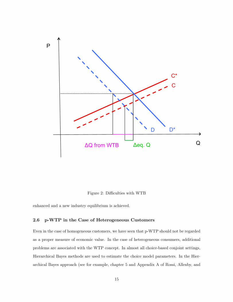
The analogous situation is shown for WTB in figure 2. We have the same cost and demand

curves, but we illustrate the WTB exercise which is to compute the change in quantity sold

assuming prices do not change. WTB clearly overstates the changes in equilibrium quantity

demanded. The figures show very clearly that both p-WTP and WTB are purely demand-

based quantities which do not take into account changes in prices and costs as the feature is

13

1"

Q

D*

P

ΔWTP

ΔEq. Price

D

C

C*

Figure 1: Difficulties with WTP

14

1"

Q

D*

P

D

C

C*

Δeq. Q ΔQ from WTB

Figure 2: Difficulties with WTB

enhanced and a new industry equilibrium is achieved.

2.6 p-WTP in the Case of Heterogeneous Customers

Even in the case of homogeneous customers, we have seen that p-WTP should not be regarded

as a proper measure of economic value. In the case of heterogeneous consumers, additional

problems are associated with the WTP concept. In almost all choice-based conjoint settings,

Hierarchical Bayes methods are used to estimate the choice model parameters. In the Hier-

archical Bayes approach (see for example, chapter 5 and Appendix A of Rossi, Allenby, and

15

McCulloch (2005)), each respondent may have different logit parameters, � and �

P

, and the

complete posterior distribution is computed for all model parameters, including individual

respondent level parameters. The problem, then, becomes how to summarize the distribu-

tion of p-WTP which is revealed via the HB analysis. The concept of p-WTP provides no

guidance as to how this distribution should be summarized. One natural summary would

be the expectation of p-WTP where the expectation is taken over the distribution of model

parameters.

E [p-WTP] =Z

�

f

�

p

p (�

f

,�

p

|Data) d�

f

d�

p

Ofek and Srinivasan (2002) propose a refinement which requires a weighted average of the

p-WTP for each consumer where the weights will depend on the probability of purchase.5

However, there is no compelling reason to prefer the mean over any other scalar summary of

the distribution of p-WTP. Some propose using a median value of p-WTP instead. Again,

there are no economic arguments as to why the mean or median or any other summary should

be preferred. The statistical properties of various summaries (e.g. mean vs. median) are

irrelevant as we are not considering the sampling performance of an estimator but rather what

is the appropriate summary of a population distribution. A proper economic valuation will

consider the entire demand curve as well as competitive and cost considerations. Equilibrium

quantities will involve the entire distribution via the first order conditions for firm profit-

maximization. These quantities cannot be expressed as a function of the mean, median or

any other simple set of scalar summaries of the distribution of p-WTP.

However, it is possible to provide a rough intuition as to why the mean of p-WTP may

be a particularly poor summary of the distribution for equilibrium computations. It is the

marginal rather than the average consumer that drive the determination of equilibrium prices.

Exactly where, in the distribution of WTP, will the marginal customer be is determined by

nature of the distribution as well as where supply factors that “slice” into the distribution of5Equation (14) on p.403 expresses the p-WTP (what the authors call MVAI) as the ratio of weighted

averages. However, in the logit model used by the authors, there is both a scale parameter and a pricecoefficient. This is not an identified model. If you include a price coefficient, then the scale parameter(denoted µ by the authors) is the negative reciprocal of the price coefficient. If substituted into (14), theMVAI expression simplifies to a weighted average of the standard p-WTP measure.

16

WTP. It is possible to construct cases where the average WTP vastly overstates the WTP

of the marginal customer. This is one of the main points of Orme (2001). If the bulk of the

market has a low value of WTP and there is a small portion of the market with extremely high

WTP (the Howells in Orme’s Gilligan’s Island metaphor), then a profit maximizing firm may

set price much lower than average WTP so as to sell to the majority of potential customers

who have relatively low WTP. There are situations where the greater volume from low WTP

consumers outweighs the high margins that might be earned from the high WTP segment.

In these cases, mean WTP will vastly overstate the price premium a firm will charge over

cost for a product. It is more difficult, but possible, to construct similar scenarios for median

WTP.

3 Economic Valuation of Features

The goal of feature enhancement is to improve profitability of the firm introducing product

with feature enhancement into an existing market. Similarly, the value of a patent is ultimately

derived from the profits that accrue to firms who practice the patent by developing products

that utilize the patented technology. In fact, standard economic argument for allowing patent

holders to sell their patents is that, in this way, patents will eventually find their way into

the hands of those firms who can best utilize the technology to maximize demand and profits.

For these reasons, we believe that the only sensible measure of the economic value of feature

enhancement is the incremental profits that the feature enhancement will generate.

�⇡ = ⇡ (p

eq

,m

eq|A⇤)� ⇡ (p

eq

,m

eq|A) (3.1)

⇡ is the profits associated with the industry equilibrium prices and shares given a particular set

of competing products which is represented by the choice set defined by the attribute matrix.

This definition allows for both price and share adjustment as a result of feature enhancement,

removing some of the objections to the p-WTP and WTB concepts. Incremental profits is

closer in spirit, though not the same, to the definition of true WTP in the sense that (3.1)

17

depends on the entire choice set and the incremental profits may depend on which product is

subject to feature enhancement. However, social WTP does not include cost considerations

and does not address how the social surplus is divided between the firm and the customers.

In the abstract, our definition of economic value of feature enhancement seems to be the

only relevant measure for the firm that seeks to enhance a feature. All funds have an op-

portunity cost and the incremental profits calculation is fundamental to deploying product

development resources optimally. In fairness, industry practitioners of conjoint analysis also

appreciate some of the benefits of an incremental profits orientation. Often marketing re-

search firms construct “market simulators” that simulate market shares given a specific set of

products in the market. Some even go further as to attempt to compute the “optimal” price

by simulating different market shares corresponding to different “pricing scenarios.” In these

exercises, practitioners fix competing prices at a set of prices that may include their informal

estimate of competitor response. This is not the same as computing a marketing equilibrium

but moves in that direction.

3.1 Assumptions

Once that principle of incremental profits is adopted, the problem becomes to define the

nature of competition, the competitive set and to choose an equilibrium concept. These

assumptions must be added to the assumptions of a specific parametric demand system (we

will use a heterogeneous logit demand system which is flexible but still parametric) as well as

a linear utility function over attributes and the assumption (implicit in all conjoint analysis)

that products can be well described by bundles of attributes. Added to these assumptions,

our valuation method will also require cost information.

Specifically, we will assume

1. Demand Specification: A standard heterogenous logit demand that is linear in the

attributes (including price)

2. Cost Specification: Constant marginal cost

18

3. Single product firms

4. Feature Exclusivity: The feature can only be added to one product

5. No Exit: Firms cannot exit or enter the market after product enhancement takes place

6. Static Nash Price Competition

Assumptions 2, 3, 4 can be easily relaxed. Assumption 1 can be replaced by any valid

or integrable demand system. Assumptions 5 and 6 cannot be relaxed without imparting

considerable complexity to the equilibrium computations.

3.2 Computing Equilibrium Prices

The standard static Nash equilibrium in a market for differentiated products is a set of prices

such that simultaneously satisfy all firms profit-maximization conditions. Each firm chooses

price to maximize firms profits, given the prices of all other firms. These conditional demand

curves are sometimes called the “best response” of the firm to the prices of other firms. An

equilibrium, if it exists,6 is a set of prices that is simultaneously the best response or profit

maximizing for each firm given the others.

In a choice setting, the firm demand is

⇡ (p

j

|p�j

) = ME [Pr (j|p,A)] (pj

� c

j

) . (3.2)

M is the size of the market, p is the vector of the prices of all J firms in the market, cj

is the

marginal cost of producing the firms product. The expectation is taken with respect to the6There is no guarantee that a Nash equilibrium exists for heterogeneous logit demand.

19

distribution of choice model parameters. In the logit case,7

E [Pr (j|p,A)] =Z

exp (�

0a

j

� �

p

p

j

)Pj

exp (�

0a

j

� �

p

p

j

)

p (�,�

p

) d�d�

p

. (3.3)

The first order conditions of the firm are

@⇡

@p

j

= E

@

@p

j

Pr (j|p,A)�(p

j

� c

j

) + E [Pr (j|p,A)] (3.4)

The Nash equilibrium price vector is a root of the system of nonlinear equations which

define the F.O.C. for all J firms. That is if we define

h (p) =

2

66666664

h1 (p) =@⇡

@p1

h2 (p) =@⇡

@p2

...

h

J

(p) =

@⇡

@pJ

3

77777775

(3.5)

then the equilibrium price vector, p⇤, is a zero of the function h (p).

There are two computational issues that arise in the calculation of Nash equilibrium prices.

First, both the firm profit function (3.2) and the FOC conditions for the firm (3.4) require the

computation of integrals to compute the expectation of the market share (market demand)

and expectation of the derivative of market share in the FOC. Second, an algorithm must

be devised for calculating the equilibrium price, given a method of approximating the inte-

grals. The most straightforward method to approximate the requisite integrals is a simulation

method. Given a distribution of demand parameters over consumers, we can approximate the

expectations by simple average of draws from this distribution. Given that both the market

share and the derivatives of market share are virtually costless to evaluate, an extremely large7We do not include a market wide shock to demand as we are not trying to build an empirical model

of market shares. We are trying to approximate the firm problem. In a conjoint setting, we abstract fromthe problem of omitted characteristics as the products we use in our market simulators are defined only interms of known and observable characteristics. Thus, the standard interpretation of the market wide shock isnot applicable here. Another interpretation is that the market wide shock represents some sort of marketingaction by the firms (e.g. advertising). Here we are directly solving the firm pricing problem holding fixed anyother marketing actions. This means that the second interpretation of the market wide shock as stemmingfrom some unobservable firm action is not applicable here.

20

number of draws can be used to approximate the integrals (we routinely use in excess of 50,000

draws).

Given the method for approximating the integral, we must choose an iterative method

for computing equilibrium prices. There are two methods available. The first is an iterative

method where we start from some price vector, compute the optimal price for each firm given

other other prices, updating the price vector as we progress from the 1st to the Jth firm.

After one cycle thru the J firms, we have updated the price vector to a second guess of the

equilibrium. We continue this process until��p

r � p

r�1��< tol. The method of iterative firm

profit maximization will work if there is a stable equilibrium. That is, if we perturb the price

vector away from the equilibrium price, the iterative process will return to the equilibrium

(at least in a neighborhood of the equilibrium). This is not guaranteed to occur even if there

is exists a unique equilibrium.

The second method for computing equilibrium prices is to find the root of set of FOCs

(3.5). The optimization problem

min

p

kh (p)k

can be solved via a quasi-Newton method which is equivalent to finding the roots directly

using Newton’s method with line search. This provides a more robust way of finding equilibria,

if they exist, but does not provide a way of finding the set of equilibria if multiple equilibria

exist. The existence of multiple equilibria would have to be demonstrated by construction

via starting the optimizer/root finder from different starting points. In our experience with

heterogeneous logit models, we have not found any instance of multiple equilibria; however

we have found situations where we cannot find any equilibria (though only rarely and for

extreme parameter values).

4 Using Conjoint Designs for Equilibrium Calculations

Economic valuation of feature enhancement requires a valid and realistic demand system as

well as cost information and assumptions about the set of competitive products. If conjoint

21

studies are to be used to calibrate the demand system, then particular care must be taken to

design a realistic conjoint exercise. The low cost of fielding and analyzing a conjoint design

makes this method particularly appealing in a litigation context. In addition, with internet

panels, conjoint studies can be fielded and analyzed in a matter of days, a time frame also

attractive in the tight schedules of patent litigation. However, there is no substitute for careful

conjoint design. Many designs fielded today are not useful for economic valuation of feature

enhancement. For example, in recent litigation, conjoint studies in which there is no outside

option, only one brand, and only patented features were used. A study with any of these

limitations is of questionable value for true economic valuation.

Careful practitioners of conjoint have long been aware that conjoint is appealing because

of it’s simplicity and low cost but that careful studies make all the difference between real-

istic predictions of demand and useless results. We will not repeat the many prescriptions

for careful survey analysis which include thorough crafting questionnaires with terminology

that is meaningful to respondents, thorough and documented pre-testing and representative

(projectable) samples. Furthermore, many of the prescriptions for conjoint design including

well-specified and meaningful attributes and levels are extremely important.8 Instead, we will

focus on the areas we feel are especially important for economic valuation and not considered

carefully enough.

4.1 Set of Competing Products

The guiding principle in conjoint design for economic valuation of feature enhancement is

that the conjoint survey must closely approximate the marketplace confronting consumers.

In industry applications, the feature enhancement has typically not yet been introduced into

the marketplace (hence the appeal of a conjoint study), while in patent litigation the survey

is being used to approximate demand conditions at some point in the past in which patent

infringement is alleged to have occurred.

Most practitioners of conjoint are aware that, for realistic market simulations, the major8See, for example, Federal Judicial Center (2011), Reference Manual on Scientific Evidence and Orme

(2009).

22

competing products must be used. This means that the product attributes in the study

should include not only functional attributes such as screen size, memory etc but also the

major brands. This point is articulated well in Orme (2001). However, in many litigation

contexts, the view is that only the products and brands accused of patent infringement should

be included in the study. The idea is that only a certain brand’s products are accused of

infringement and, therefore, that the only relevant feature enhancement for the purposes of

computing patent damages are feature enhancement in the accused products.

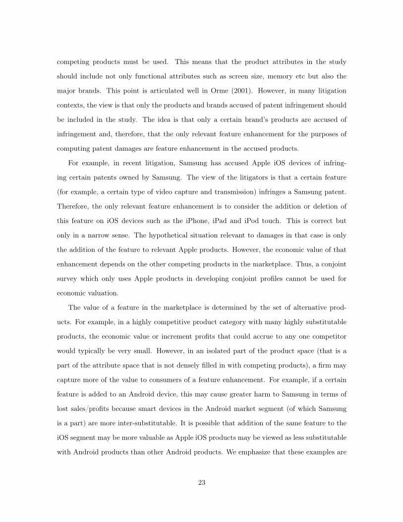
For example, in recent litigation, Samsung has accused Apple iOS devices of infring-

ing certain patents owned by Samsung. The view of the litigators is that a certain feature

(for example, a certain type of video capture and transmission) infringes a Samsung patent.

Therefore, the only relevant feature enhancement is to consider the addition or deletion of

this feature on iOS devices such as the iPhone, iPad and iPod touch. This is correct but

only in a narrow sense. The hypothetical situation relevant to damages in that case is only

the addition of the feature to relevant Apple products. However, the economic value of that

enhancement depends on the other competing products in the marketplace. Thus, a conjoint

survey which only uses Apple products in developing conjoint profiles cannot be used for

economic valuation.

The value of a feature in the marketplace is determined by the set of alternative prod-

ucts. For example, in a highly competitive product category with many highly substitutable

products, the economic value or increment profits that could accrue to any one competitor

would typically be very small. However, in an isolated part of the product space (that is a

part of the attribute space that is not densely filled in with competing products), a firm may

capture more of the value to consumers of a feature enhancement. For example, if a certain

feature is added to an Android device, this may cause greater harm to Samsung in terms of

lost sales/profits because smart devices in the Android market segment (of which Samsung

is a part) are more inter-substitutable. It is possible that addition of the same feature to the

iOS segment may be more valuable as Apple iOS products may be viewed as less substitutable

with Android products than other Android products. We emphasize that these examples are

23

simply conjectures to illustrate the point that a full set of competing products must be used

in the conjoint study. However, we do not think it necessary to have all possible product vari-

ants or competitors in the conjoint study and subsequent equilibrium computations. In many

product categories, this would require a massive set of possible products with many features.

Our view is that it is important to design the study to consider the major competing products

both in terms of brands and the attributes used in the conjoint design. It is not required that

the conjoint study exactly mirror the complete set of products and brands that are in the

marketplace but that the main exemplars of competing brands and product positions must

be included.

4.2 Outside Option

There is considerable debate as to the merits of including an outside option in conjoint studies.

Many practitioners use a “forced-choice” conjoint design in which respondents are forced to

choose one from the set product profiles in each conjoint choice task. The view is that

“forced-choice” will elicit more information from the respondents about the tradeoffs between

product attributes. If the “outside” or “none of the above” option is included, advocates of

forced choice argue that respondents may shy away from the cognitively more demanding task

of assessing tradeoffs and select the “none” option to reduce cognitive effort. On the opposite

side, other practitioners advocate inclusion of the outside option in order to assess whether

or not the product profiles used in the conjoint study are realistic in the sense of attracting

considerable demand. The idea being that if respondents select the “none of the above”

option too frequently then the conjoint design has offered very unattractive hypothetical

products. Still others (see, for example, Brazell, Diener, Karniouchina, Moore, Severin, and

Uldry (2006)) argue the opposite side of the argument for forced choice. They argue that

there is a “demand” effect in which respondents select at least one product to “please” the

investigator. There is also a large literature on how to implement the “outside” option.

Whether or not the outside option is included depends on the ultimate use of the conjoint

study. Clearly, it is possible to measure how respondents trade-off different product attributes

24

against each other without inclusion of the outside option. For example, it is possible to

estimate the price coefficient in a conjoint study which does not include the outside option.

Under the assumption that all respondents are NOT budget constrained, the price coefficient

should theoretically measure the trade-offs between other attributes and price. The fact

that respondents might select a lower price and pass on some features means that they have

an implicit valuation of the dollar savings involved in this trade-off. If all respondents are

standard economic agents, then this valuation of dollar savings is a valid estimate of the

marginal utility of income. This means that a conjoint study without the outside option can

be used to compute the p-WTP measure (2.3) which only requires a valid price coefficient.

We have argued that p-WTP is not a measure of the economic value to the firm of feature

enhancement. This requires a complete demand system (including the outside good) as well

as the competitive and cost conditions. In order to compute valid equilibrium prices, we need

to explicitly consider substitution from and to other goods including the outside good. For

example, suppose we enhance a product with a very valuable new feature. We would expect

to capture sales from other products in the category as well as to expand the category sales;

the introduction of the Apple iPad dramatically grew the tablet category due, in part, to the

features incorporated in the iPad. Chintagunta and Nair (2011) make a related observation

that price elasticities will be biased if the outside option is not included.

We conclude that an outside option is essential for economic valuation of feature enhance-

ment as the only way to incorporate substitution in and out of the category is by the addition

of the outside option. At this point, it is possible to take the view that if respondents are

pure economic actors that they should select the outside option corresponding to their true

preferences and that their choices will properly reflect the marginal utility of income. How-

ever, there is a growing literature which suggests that different ways of expressing or allowing

for the outside option will change the frequency with which it is selected. In particular, the

so-called “dual response” way of allowing for the outside option (see Uldry, Severin, and Diener

(2002) and Brazell, Diener, Karniouchina, Moore, Severin, and Uldry (2006)) has been found

to increase the frequency of selection of the outside option. The “dual-response” method asks

25

the respondent first to indicate which of the product profiles (without the outside option) are

most preferred and then asked if the respondent would actually buy the product at the price

posted in the conjoint design. Our own experience confirms that this mode of including the

outside option greatly increases the selection of the outside option. Our experience has also

been that the traditional method of including the outside option often elicits a very low rate

of selection which we view as unrealistic. The advocates of the “dual response” method argue

that the method helps to reduce a conjoint survey bias toward higher purchase rates than in

the actual marketplace.

Another way of reducing bias toward higher purchase rates is to design a conjoint using

an “incentive-compatible” scheme in which the conjoint responses have real monetary conse-

quences. There are a number of ways to do this (see, for example, Ding, Grewal, and Liechty

(2005)) but most suggestions (an interesting exception is Dong, Ding, and Huber (2010)) use

some sort of actual product and a monetary allotment. If the products in the study are actual

products in the marketplace, then the respondent might actually receive the product chosen

(or, perhaps, be eligible for a lottery which would award the product with some probability).

If the respondent selects the outside option, they would receive a cash transfer (or equivalent

lottery eligibility).

5 Statistical Inference for Economic Valuation

Bayesian Hierarchical models are now by far the dominant method for use in analysis of

choice-based conjoint data. The leading vendors9 of statistical software designed to analyze

choice-based conjoint data both feature implementations of MCMC methods for hierarchical

logit models. We will not review these approaches, but, instead, consider some important

points relevant to the economic valuation method.9Sawtooth Software and SAS Institute

26

5.1 Individual or Market Quantities?

The appeal of Bayesian methods is based primarily on the ability to produce inferences at the

respondent level as well as to free statistical inference from asymptotic approximations which

are dubious at best in conjoint exercises where very few (invariably less than 20) observations

are collected per respondent. However, there has been a great deal of confusion as to how

to develop and use respondent level inferences. Many simply compute Bayesian estimates at

the respondent level based on averages of the MCMC draws of the parameter vector at the

respondent level.

ˆ

�

i

=

1

R

X

r

�

r

i

(5.1)

Here i is the index of the respondent and r is the index of the MCMC draws for that re-

spondent. While there is nothing inherently wrong with this estimate, the distribution of

these estimates across respondents is not a valid estimate of true distribution of preference

or part-worth parameters than constitutes the market. Intuitively, we all know that there

is a great deal of uncertainty in the respondent level parameter estimates as they are based

only on a handful of observations and the Bayes procedures do not borrow a great deal of

strength from other observations unless the distribution of heterogeneity is inferred to be very

tight. These problems are magnified for the p-WTP measure which is a ratio of logit param-

eters. It is a violation of coherent Bayesian inference to take the ratio of respondent-level

estimates and use the distribution of this ratio across respondents as valid inference for the

population distribution of p-WTP. This ad hoc procedure will not only introduce bias but

also mis-represent the true uncertainty in our inference regarding the mean of p-WTP in the

population of consumers.

Instead of focusing on individual estimates and exposing the attendant problems with

these estimates, economic valuation forces the investigator to estimate the distribution of

tastes which is then used to compute market demand. To review, if we know the distribution

of part-worths (preferences) over respondents we can compute market demand for any firm’s

27

product as

MS (j) =

ZPr (j|�) p (�) d�. (5.2)

Here MS(j) is the market share of product j. However, we do not know the exact distribution of

preferences. What we have is a model for preferences (the first stage of the hierarchical model)

and inferences about the parameters of this model. A proper Bayesian analysis would conduct

posterior inference on any market wide quantity (such as market share, market-wide p-WTP,

first order conditions of the firm which are based on market demand, etc). To compute the

posterior distribution of a quantity like market share, we begin with the assumptions in the

hierarchical model. Typically, we assume that the model parameters (or some transform of

them) is normally distributed.

p (�) = � (�|µ, V�

) (5.3)

Here � (•) is the multivariate normal density. This means that market share defined in (5.2)

is function of the hyper-parameters that govern the normal, first-stage or random coefficient,

distribution.

MS (j|µ, V�

) =

ZPr (j|�)� (�|µ, V

�

) d� (5.4)

To compute the posterior predictive distribution of market share, we must integrate (5.4)

with respect to the posterior distribution of the hyper-parameters.

p (MS (j) |data) =Z

MS (j|µ, V�

) p (µ, V

�

|data) dµ dV

�

(5.5)

Thus, the posterior predictive distribution of market share or any other market wide quantity

can easily be computed from posterior draws of the hyper-parameters. We simply draw from

the multivariate normal density given each draw of the hyper-parameters to obtain a draw

from the relevant posterior predictive distribution.

MS (j)

r

=

ZPr (j|�)�

��|µr

, V

r

�

�d� (5.6)

This idea can be used to compute the posterior distribution of any quantity including

28

the posterior distribution of equilibrium prices as equilibrium prices are also a function of

the random coefficient parameters. In the illustration of our method, we will take all of the

draws of the normal hyper-parameters and then for each draw we will solve for the equilibrium

prices. This will build up the correct posterior distribution of equilibrium quantities.

5.2 Estimating Price Sensitivity

Both p-WTP and equilibrium prices are sensitive to inferences regarding the price coefficient.

If the distribution of prices puts any mass at all on positive values, then there does not exist

a finite equilibrium price. All firms will raise prices infinitely, effectively firing all consumers

with negative price sensitivity and make infinite profits on the segment with positive price

sensitivity. Most investigators regard positive price coefficients as inconsistent with rational

behavior. However, it will be very difficult for a normal model to drive the mass over the

positive half line for price sensitivity to a negligible quantity if there is mass near zero on the

negative side. We must distinguish uncertainty in posterior inference from irrational behavior.

If a number of respondents have posteriors for price coefficients that put most mass on positive

values, this suggests a design error in the conjoint study; perhaps, respondents are using price

an a proxy for the quality of omitted features and ignoring the “all other things equals” survey

instructions. In this case, the conjoint data should be discarded and the study re-designed.

On the other hand, we find considerable mass on positive values simply because of the normal

assumption and the fact that we have very little information about each respondent. In these

situations, we have found it helpful to change the prior or random effect distribution to impose

a sign constraint on the price coefficient.

2

64�

�

⇤p

= ln (��

p

)

3

75 ⇠ N (µ, V

�

) (5.7)

Given that a RW-Metropolis step is used to draw logit parameters, this re-parameterization

can be implemented trivially in the evaluation of the likelihood function only. The only change

that should be made is in the assessment of the IW prior on V

�

. In the default settings, we

29

use a relatively diffuse prior, V�

⇠ IW (⌫, ⌫V ), with V = I. We must recognize that the price

element of � is now on a log-scale and it would be prudent to lower the prior diffusion to a

more modest level such as .05 rather than leaving that diagonal element at 1.0. It should be

noted that the prior outlined here will have a zero probability of a price coefficient which is

� 0. This is not true for more ad hoc methods such as the method of “tie-breaking” used in

Sawtooth Software.

Even with a prior that only puts positive mass only on negative values, there may still be

difficulties in computing sensible equilibrium prices due to a mass of consumers with negative

but very small price sensitivities. Effectively this will flatten out the profit function for each

firm and make it difficult to find an equilibrium solution. The lower the curvature of the profit

function, the more sensitive the profit function (or first order conditions) will be to simulation

error in the approximation of the integrals. In our illustration in section 6, we do not find

this problem but it is a potential problem with many conjoint studies.

In many conjoint studies, the goal is to simulate market shares for some set of products.

Market shares can be relatively insensitive to the distribution of the price coefficients when

prices are fixed to values typically encountered in the marketplace. It is only when one

considers relative prices that are unusual or relatively high or low prices that the implications

of a distribution of price sensitivity will be felt. By definition, price optimization will stress-

test the conjoint exercise by considering prices outside the small range usually consider in

market simulators. For this reason, the quality standards for design and analysis of conjoint

data have to be much higher when used from economic valuation than for many of the typical

uses for conjoint. Unless the distribution of price sensitivity puts little mass near zero, the

conjoint data will not be useful for economic valuation using either our equilibrium approach

or for the use of the more traditional and flawed p-WTP methods.

6 An Illustration Using the Digital Camera Market

To illustrate our proposed method for economic valuation and to contrast our method with

standard p-WTP methods, we consider the example of the digital camera market. We designed

30

a conjoint survey to estimate the demand for features in the point and shoot submarket. We

considered the following seven features with associated levels:

1. Brand: Canon, Sony, Nikon, Panasonic

2. Pixels: 10, 16 mega-pixels

3. Zoom: 4x, 10x optical

4. Video: HD (720p), Full HD (1080p) and mike

5. Swivel Screen: No, Yes

6. WiFi: No, Yes

7. Price: $79-279

We focused on evaluating the economic value of the swivel screen feature which is illustrated

in Figure 3. The conjoint design was a standard fractional factorial design in which each

respondent viewed sixteen choice sets, each of which featured four hypothetical products.

A dual response mode was used to incorporate the outside option. Respondents were first

asked which of the four profiles presented in each choice task was most preferred. Then

the respondent was asked if they would buy the preferred profile at the stated price. If no,

then this response is recorded as the “outside option” or “none of the above.” Respondents

were screened to only those who owned a point and shoot digital camera and who considered

themselves to be a major contributor to the decision to purchase this camera.

The survey was fielded to the Sampling Surveys International internet panel in August

2013. We received 501 completed questionnaires.10 We recorded time to complete the conjoint

portion of the survey. The median time to complete is 220 seconds or about 14 seconds per

conjoint task. The 25th percentile is 151 seconds and the 75th percentile is 333 seconds.10This study was part of a wave of four other very similar conjoint studies on digital cameras each with

the same screening criteria. For all studies in the wave, 16,185 invitations were sent to panelists, 6,384responded. Of those who responded to the invitation, 2,818 passed screening and of those passing screening2,503 completed the questionnaire. Thus, the overall completion rate is 89 per cent which is good by surveystandards.

31

Figure 3: Swivel Screen Attribute

To check sensitivity to time spent on the survey, we conducted analyses deleting the bottom

quartile of the respondents and found little change. It is a common and well-accepted practice

to remove respodents who “straight-line” or always select the same option (such as the left

most choice). The idea is that these “straightliners” are not putting sufficient effort into the

choice task. Of our 501 complete questioniares, only 2 respondents displayed straightline

behavior and were eliminated. We also eliminated 6 respondents who always selected the

same brand and two respondents who always selected the high price brand. Our reasoning is

that these respondents did not appear to be taking the trade-offs conjoint exercise seriously.

We also eliminated 23 respondents who always selected the outside option as their part-worths

are not identified without prior information. Thus, our final sample sie was 468 out of an

original size of 501.

To analyze the conjoint data, we use the bayesm routine rhierMnlMixture. We employed

standard diffuse prior settings as discussed in section 5 and 50,000 MCMC draws were made.

The first 10,000 draws were discarded for burn-in purposes. The hierarchical model we em-

ployed assumes that the conjoint price-worths are normally distributed. We can compute the

posterior predictive distribution of part-worths as follows:

p (�|data) =Z

� (�|µ, V�

) p (µ, V

�

|data) dµ dV

�

(6.1)

(6.1) shows the influence of both the model (the normal random coefficient distribution) and

the data through the posterior distribution of the normal hyper-parameters. The resulting

32

Price\Mkt Share MSSony

MSCanon

MSNikon

MSPansonic

P

Sony

-1.69 .50 .36 .34P

Canon

.53 -1.79 .37 .44P

Nikon

.40 .39 -1.56 .28P

Panasonic

.46 .55 .34 -1.73

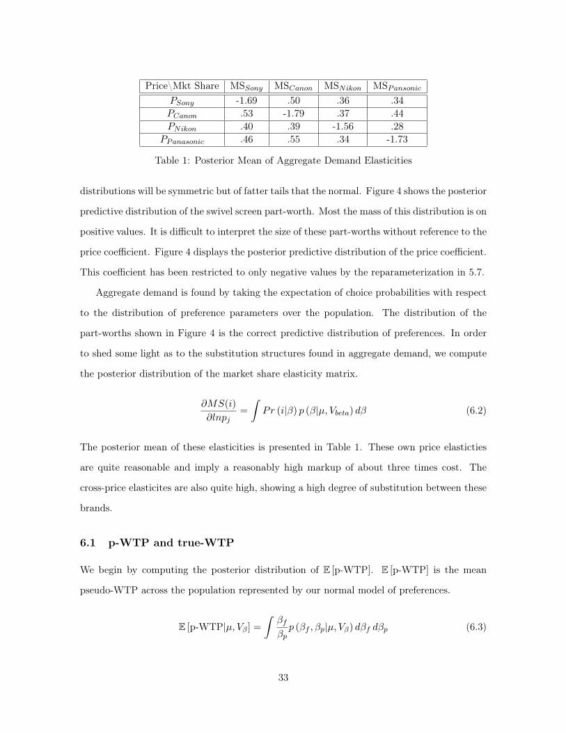
Table 1: Posterior Mean of Aggregate Demand Elasticities

distributions will be symmetric but of fatter tails that the normal. Figure 4 shows the posterior

predictive distribution of the swivel screen part-worth. Most the mass of this distribution is on

positive values. It is difficult to interpret the size of these part-worths without reference to the

price coefficient. Figure 4 displays the posterior predictive distribution of the price coefficient.

This coefficient has been restricted to only negative values by the reparameterization in 5.7.

Aggregate demand is found by taking the expectation of choice probabilities with respect

to the distribution of preference parameters over the population. The distribution of the

part-worths shown in Figure 4 is the correct predictive distribution of preferences. In order

to shed some light as to the substitution structures found in aggregate demand, we compute

the posterior distribution of the market share elasticity matrix.

@MS(i)

@lnp

j

=

ZPr (i|�) p (�|µ, V

beta

) d� (6.2)

The posterior mean of these elasticities is presented in Table 1. These own price elasticties

are quite reasonable and imply a reasonably high markup of about three times cost. The

cross-price elasticites are also quite high, showing a high degree of substitution between these

brands.

6.1 p-WTP and true-WTP

We begin by computing the posterior distribution of E [p-WTP]. E [p-WTP] is the mean

pseudo-WTP across the population represented by our normal model of preferences.

E [p-WTP|µ, V�

] =

Z�

f

�

p

p (�

f

,�

p

|µ, V�

) d�

f

d�

p

(6.3)

33

Price Part−Worth

−10 −8 −6 −4 −2 0

Swivel Screen Part−Worth

−4 −2 0 2 4 6

Figure 4: Posterior Predictive Distribution of Price and Swivel Screen Part-Worths

34

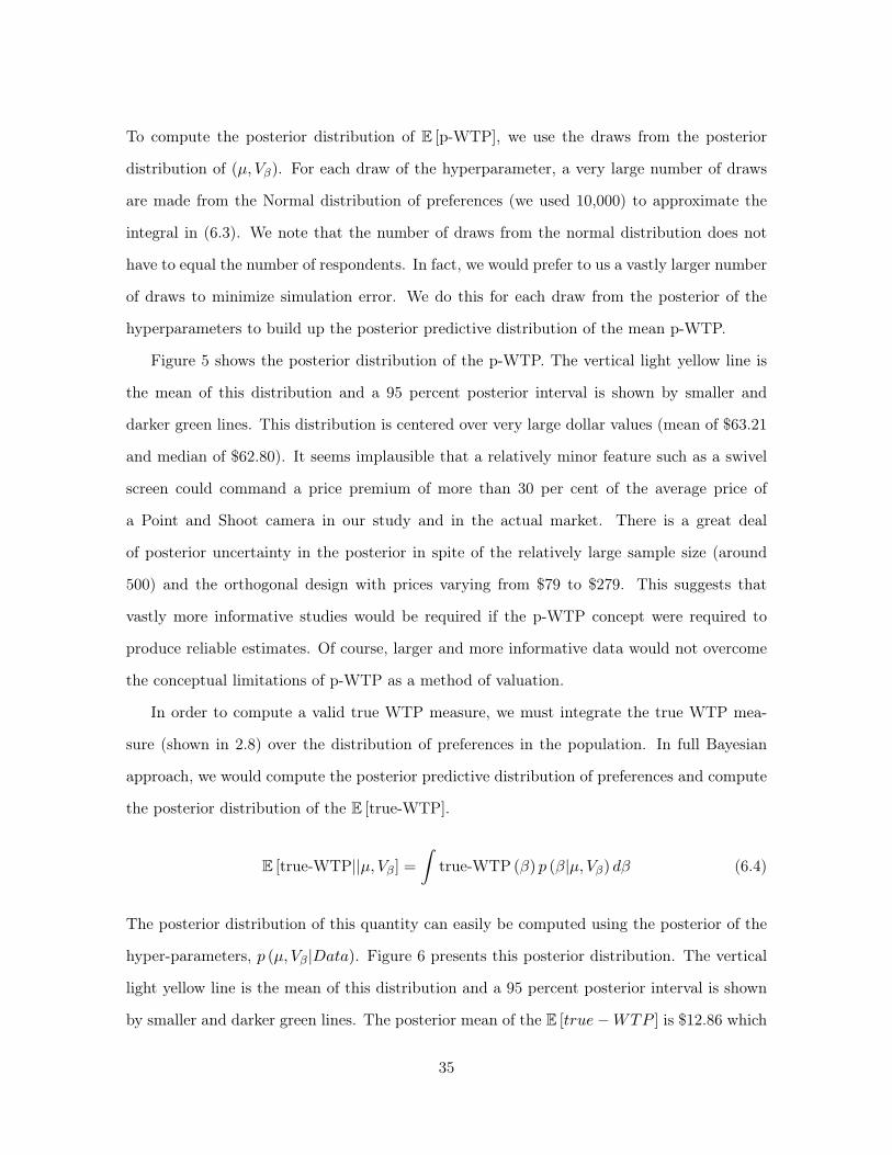
To compute the posterior distribution of E [p-WTP], we use the draws from the posterior

distribution of (µ, V�

). For each draw of the hyperparameter, a very large number of draws

are made from the Normal distribution of preferences (we used 10,000) to approximate the

integral in (6.3). We note that the number of draws from the normal distribution does not

have to equal the number of respondents. In fact, we would prefer to us a vastly larger number

of draws to minimize simulation error. We do this for each draw from the posterior of the

hyperparameters to build up the posterior predictive distribution of the mean p-WTP.

Figure 5 shows the posterior distribution of the p-WTP. The vertical light yellow line is

the mean of this distribution and a 95 percent posterior interval is shown by smaller and

darker green lines. This distribution is centered over very large dollar values (mean of $63.21

and median of $62.80). It seems implausible that a relatively minor feature such as a swivel

screen could command a price premium of more than 30 per cent of the average price of

a Point and Shoot camera in our study and in the actual market. There is a great deal

of posterior uncertainty in the posterior in spite of the relatively large sample size (around

500) and the orthogonal design with prices varying from $79 to $279. This suggests that

vastly more informative studies would be required if the p-WTP concept were required to

produce reliable estimates. Of course, larger and more informative data would not overcome

the conceptual limitations of p-WTP as a method of valuation.

In order to compute a valid true WTP measure, we must integrate the true WTP mea-

sure (shown in 2.8) over the distribution of preferences in the population. In full Bayesian

approach, we would compute the posterior predictive distribution of preferences and compute

the posterior distribution of the E [true-WTP].

E [true-WTP||µ, V�

] =

Ztrue-WTP (�) p (�|µ, V

�

) d� (6.4)

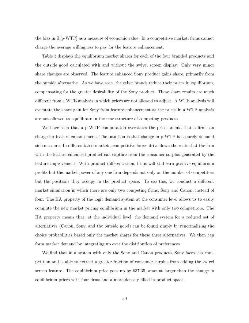
The posterior distribution of this quantity can easily be computed using the posterior of the

hyper-parameters, p (µ, V�

|Data). Figure 6 presents this posterior distribution. The vertical

light yellow line is the mean of this distribution and a 95 percent posterior interval is shown

by smaller and darker green lines. The posterior mean of the E [true�WTP ] is $12.86 which

35

0 50 100 150| |Figure 5: Posterior Distribution of E [p-WTP]

is much lower than the p-WTP measure. This is because the true-WTP measure integrates

over the possible realizations of the random utility errors which diminishes the effect of the

increase in mean utility for any one alternative.

6.2 Changes in Equilibrium Prices and Shares

We have argued that economic value should be expressed as incremental profits that accrue

to the firm that engages in feature enhancement. It is difficult to provide a realistic base or

scaling for firm profits without more information regarding market size and cost. However,

we can compute equilibrium prices with and without feature enhancement to provide an idea

36

5 10 15 20 25 30| |

Figure 6: Posterior Distribution of E [true-WTP]

37

Sony Canon Nikon PanasonicW/O SS $173.68 $188.44 $211.44 $182.40W SS $208.64 $183.77 $199.63 $176.53� $34.96 -$4.67 -$11.81 -$5.87

Table 2: Changes in Equilibrium Prices

of how much the focal firm can charge as a price premium and how market shares will adjust

in the new industry equilibrium. Here we consider the change in equilibrium outcomes from

adding the swivel screen display to the Sony base product (a Sony brand camera with all

attributes turned to their “lowest” value except, of course, price which is not constrained).

The value conferred by the addition of the swivel screen with also depend on the configuration

of other competing products. For illustration purposes only, we considered a competitive set

that consists of three other brands (Canon, Nikon, and Panasonic) all similarly configured at

the “base” level of attributes. We set the marginal cost of product for all brands to be $75.

When the Swivel Screen feature is added, we assume marginal cost is increased by $5 to $80.

Table 2 presents the posterior means of the equilibrium prices computed with and without

the swivel screen addition to the Sony product.11 As we might expect, adding the swivel screen

gives the Sony brand more effective market power relative to the other branded competitors

who do not have the feature (note: we could have easily simulated a competitive reaction in

which some or all of the other brands adopted the feature). Not only does Sony find it optimal

to raise price, the stronger competition and diminished value of the other brands forces them

to lower prices in equilibrium.

Given our finding that inference about p-WTP is imprecise, we might be concerned that

the same is true for the change in equilibrium prices which we are interpreting as what Sony

can charge for the feature enhancement in the marketplace. Figure 7 plots the posterior distri-

bution of the change in equilibrium price. This distribution is much more tightly distributed

around the mean of $34.96, represented by the vertical yellow bar. The green vertical bars

along the horizontal axis represent a 95 per cent posterior interval. Even the right most end

point of this interval is not near the posterior mean of E [p-WTP]. This clearly demonstrates11The numbers displayed in the table are posterior means.

38

the bias in E [p-WTP] as a measure of economic value. In a competitive market, firms cannot

charge the average willingness to pay for the feature enhancement.

Table 3 displays the equilibrium market shares for each of the four branded products and

the outside good calculated with and without the swivel screen display. Only very minor

share changes are observed. The feature enhanced Sony product gains share, primarily from

the outside alternative. As we have seen, the other brands reduce their prices in equilibrium,

compensating for the greater desirability of the Sony product. These share results are much

different from a WTB analysis in which prices are not allowed to adjust. A WTB analysis will

overstate the share gain for Sony from feature enhancement as the prices in a WTB analysis

are not allowed to equilibrate in the new structure of competing products.

We have seen that a p-WTP computation overstates the price premia that a firm can

charge for feature enhancement. The intuition is that change in p-WTP is a purely demand

side measure. In differentiated markets, competitive forces drive down the rents that the firm

with the feature enhanced product can capture from the consumer surplus generated by the

feature improvement. With product differentiation, firms will still earn positive equilibrium

profits but the market power of any one firm depends not only on the number of competitors

but the positions they occupy in the product space. To see this, we conduct a different

market simulation in which there are only two competing firms, Sony and Canon, instead of

four. The IIA property of the logit demand system at the consumer level allows us to easily

compute the new market pricing equilibrium in the market with only two competitors. The

IIA property means that, at the individual level, the demand system for a reduced set of

alternatives (Canon, Sony, and the outside good) can be found simply by renormalizing the

choice probabilities based only the market shares for these three alternatives. We then can

form market demand by integrating up over the distribution of preferences.

We find that in a system with only the Sony and Canon products, Sony faces less com-

petition and is able to extract a greater fraction of consumer surplus from adding the swivel

screen feature. The equilibrium price goes up by $37.35, amount larger than the change in

equilibrium prices with four firms and a more densely filled in product space.

39

Sony Canon Nikon Panasonic Outside GoodW/O SS 13% 13% 11% 10% 53%W SS 14% 13% 11% 10% 52%� 1% -1%

Table 3: Changes in Equilibrium Shares

20 40 60 80 100 120| |

Figure 7: Posterior Distribution of the Change in Sony Equilibrium Price

40

6.3 Comparison of Change in Equilibrium Shares to a WTB Analysis

As discussed in section 2, a WTB analysis holds prices fixed and examines how market share

may increase with the addition of a product feature. We have emphasized that a WTB

analysis will overstate share gains as, in equilbrium, prices will adjust and this will reduce

the share effects. To illustrate this, we consider a WTB analysis for the Sony product. In

Table 3, we show that when the Swivel Screen product is added to the Sony brand there is an

increase in equilibrium price of around $34 but that, in the new equilibrium, the Sony share

increase by only one per cent. To undertake the WTB computations, we hold price fixed at

the equilibrium that prevails without the Swivel Screen enhancement and we compute the

posterior predictive distribution of the difference in market share for the Sony product with

and without the Swivel Screen. Figure 8 show this distribution. The mean WTB share change

is about 5.5 share points more than five times the change in equilbrium share. Moreover, the

posterior interval for this change in share does not even extend much below 4 share points, far

above the equilibrium change. This shows that a WTB analysis can dramatically overstate

share or sales changes due to feature enhancement.

7 Conclusions

Valuation of product features is an important part of the development and marketing of new

products as well as the valuation of patents which are related to feature enhancement. We take

the position that the only sensible measure of the economic value of a feature enhancement

(either the addition of a completely new feature or the enhancement of an existing feature) is

incremental profits. That is, we compare the equilibrium outcomes in a marketplace in which

one of the products (corresponding to the focal firm) is feature enhanced with the equilibrium

profits in the same marketplace but where the focal firm’s product is not feature enhanced.

This measure of economic value can be used to make decisions about the development of new

features or to choose between a set of feature that could be enhanced. In the patent litigation

setting, the value of the patent as well as the damages that may have occurred due to patent

41

0.03 0.04 0.05 0.06 0.07 0.08| |

Figure 8: Posterior Distribution of the Change in Sony Share: WTB Analysis

42

infringement should be based on an incremental profits concept.

Conjoint studies can play a vital role in feature valuation provided that they are properly

designed, analyzed, and supplemented by information on the competitive and cost structure

of the marketplace in which the feature-enhanced product is introduced. Conjoint methods

can be used to develop a demand system but require careful attention to the inclusion of the

outside option and inclusion of the relevant competing brands. Proper negativity constraints

must be used to restrict the price coefficients to negative values. In addition, the Nash

equilibrium prices computed on the basis of the conjoint-constructed demand system are

sensitive to the precision of inference with respect to price sensitivity. This may mean larger

and more informative samples than typically used in conjoint applications today.

We explain why the current practice of using a change in “WTP” as a way valuing a

feature is not a valid measure of economic value. In particular, the calculations done today

involving dividing the part-worths by the price coefficient are not even proper measures of

WTP. Current pseudo-WTP measures have a tendency to overstate the economic value of

feature enhancement as they are only measures of shifts in demand and do not take into

account the competitive response to the feature enhancement. In general, firms competing

against the focal feature-enhanced product will adjust their prices downward in response to

the more formidable competition afforded by the feature enhanced product. In addition,

WTB analyses will also overstate the effects of feature enhancement on market share or sales

as these analyses also do not take into account the fact that a new equilibrium will prevail in

the market after feature enhancement takes place.

We illustrate our method by an application in the point and shoot digital camera market.

We consider the addition of a swivel screen display to a point and shoot digital camera

product. We designed a fielded a conjoint survey with all of the major brands and other

major product features. Our equilibrium computations show that the economic value of the

swivel screen is substantial and discernible from zero but about one half of the pseudo WTP

measure commonly employed. In the standard WTB analysis, prices are held fixed and the

increase in market share is computed from addition of a feature. We show that WTB analysis

43

overstates changes in market share by more than five times the change in equilibrium share.

44

References

Brazell, J., C. Diener, E. Karniouchina, W. Moore, V. Severin, and P.-F. Uldry

(2006): “The No-Choice Option and Dual Response Choice Designs,” Marketing Letters,

17(4), 255–268.

Chintagunta, P., and H. Nair (2011): “Discrete-Choice Models of Consumer Demand in

Marketing,” Marketing Science, 30(6), 977–996.

Ding, M., R. Grewal, and J. Liechty (2005): “Incentive-Aligned Conjoint,” Journal of

Marketing Research, 42(1), 67–82.

Dong, S., M. Ding, and J. Huber (2010): “A Simple Mechanism to Incentive-align Conjoint

Experiments,” International Journal of Research in Marketing, 27(25-32).

Green, P. E., and Y. Wind (1989): “Courtyard by Marriott: Designing a Hotel Facility

with Consumer-based marketing Models,” Interfaces, 19(1), 25–47.

Gustafsson, A., A. Herrmann, and F. Huber (eds.) (2000): Conjoint Measurement:

Methods and Applications. Springer-Verlag.

McFadden, D. L. (1981): “Econometric Models of Probabilistic Choice,” in Structural Anal-

ysis of Discrete Choice, ed. by M. Intrilligator, and Z. Griliches, pp. 1395–1457. North-

Holland.

Ofek, E., and V. Srinivasan (2002): “How Much Does the Market Value an Improvement

in a Product Attribute,” Marketing Science, 21(4), 398–411.

Orme, B. K. (2001): “Assessing the Monetary Value of Attribute Levels with Conjoint

Analysis,” Discussion paper, Sawtooth Software, Inc.

Orme, B. K. (2009): Getting Started with Conjoint Analysis. Research Publishers, LLC.

Rossi, P. E., G. M. Allenby, and R. E. McCulloch (2005): Bayesian Statistics and

Marketing. John Wiley & Sons.

45

Sonnier, G., A. Ainslie, and T. Otter (2007): “Heterogeneity Distributions of

Willingness-to-Pay in Choice Models,” Quantitative Marketing and Economics, 5, 313–331.

Trajtenberg, M. (1989): “The Welfare Analysis of Product Innovations, with an Applica-

tion to Computed Tomography Scanners,” Journal of Political Economy, 97(2), 444–479.

Uldry, P., V. Severin, and C. Diener (2002): “Using a Dual Response Framework in

Choice Modeling,” in AMA Advanced Research Techniques Forum.

Viscusi, W. K., and J. Huber (2012): “Reference-dependent Valuations of Risk: Why

willingness-to-accept exceeds willingness-to-pay,” Journal of Risk and Uncertainty, 44, 19–

44.

46