Embed Size (px)
Citation preview

1
ECONOMIC POTENTIAL OF DEMAND SIDE MANAGEMENT IN AN INDUSTRIALIZED COUNTRY – THE CASE OF GERMANY
Dipl.-Wi.-Ing. Moritz Paulus Institute of Energy Economics (EWI)
at the University of Cologne Albertus-Magnus-Platz
50923 Cologne [email protected]
Dipl.-Wi.-Ing. Frieder Borggrefe Institute of Energy Economics (EWI)
at the University of Cologne Albertus-Magnus-Platz
50923 Cologne [email protected]
Abstract This paper provides results from a model-based analysis of long-term investments into Demand Side Management (DSM) potentials for the German power market. The paper investigates the impact of investments in DSM technologies on the reserve and spot markets in Germany up to the year 2020. Model input is an array of technical potentials from industrial processes as well as household appliances with relevant potential for load reduction, which are identified in the first part of the paper. Calibration of technical properties and long term technical capacity potentials are based on an analysis of German household appliances by Stadler (2006) as well as a thorough industry survey by Borggrefe and Paulus (2009). Both household and industrial potentials show opposing cost structure with high investments and low variable costs for household DSM and low investments and high variable costs in industrial DSM. The model extends the European electricity market simulation DIME and determines the impact on cost of electricity supply and overall DSM potentials. We discover that investment costs and opportunity costs for lost load restrict Demand Side Management mostly to the tertiary reserve capacity markets up to 2020. Nevertheless, total system cost savings through DSM are expected to amount to 0.5 bn € up to the year 2020. Keywords: Demand Side Management, integration of renewable energies, load shedding, load shifting, peak shaving, valley filling, value of lost load, energy intensive industries
Introduction Installed wind capacity in Europe is expected to rise from today’s figure of 57.2 GW, to 226.7 GW in 2020 (Benston, 2008). The current volatility in forecasted wind supply already affects European electricity systems (Auer et al. 2005). Wind supply uncertainties further affect the reserve capacities and demand for balancing power to ensure reliable electricity generation (Brückel et al. 2006, Geiger et al. 2004). A large study of the transmission system operators (TSO) and the German Energy Agency (Bartels et al., 2006) showed that despite of improved wind forecasts, increased wind capacities will lead to a growing demand for positive and negative balancing power in Germany. By 2015 the maximum hourly demand for positive and negative regulating power will threefold compared to 2003. The sharp increase in an in general highly stochastic wind energy feed-in will have significant effects on the shape of the residual load curve which the conventional power plant fleet has to satisfy. The residual load curve will become more and more volatile and therefore disadvantageous. Furthermore the annual load duration curve will become steeper. Such volatile residual load curve poses higher requirements on the flexibility of the conventional power plant fleet in order to rapidly increase or decrease load according to the current deviations of actual wind energy feed-in from the day-ahead forecasted and thus expected feed-in. Flexibility options include increased investments into generation such as more gas turbines or investing into electricity storage options such as pump storages or
2
compressed air energy storages (CAES). One alternative option does not affect the supply side in the electricity supply chain, but the demand side. This flexibility option is referred to as Demand Side Management (DSM).1 DSM exploits flexibilities in power demand by forwarding real-time price data to the customers. There are several scenarios of how this can be realized, some including a so-called „traffic light“ approach where the customer decides whether to reduce his power demand or not. Another approach is that of full automation by installing energy management systems and smart meters. In this option, the customer is not involved in the decision of whether to reduce load or not. The latter approach will be investigated in this article, because only these DSM measures might be able to provide balancing power. Key question in this paper is to determine how cost efficient and how effective are the different DSM flexibility options in a competitive market. In this context effectiveness is defined as the magnitude of flexibility provided and cost-efficiency is understood as the monetary effort necessary to bring specific flexibility option to life. There has been only very little research on German potentials as well as cost estimates for DSM with respect to balancing markets . Stadler (2006) investigated an exhaustive number of industrial processes and household appliances. However, he focused on technical potentials, thus the question of the overall magnitude of existing flexibility options, while leaving out any economic analysis of these technologies. Klobasa (2007) considered not only the potential magnitude of Demand Side Management but also investigated possible cost savings coming from additional flexibility in the electricity system through DSM technologies. His approach is based on a dispatch model for the German electricity market where the technical potentials of different DSM processes are treated as exogenous parameters to the model. The delta of the total system cost function could then be interpreted as monetary value of such additional flexibility in the system. However, Klobasa (2007) did not investigate the question of how investments into DSM potentials develop and what technologies are likely to be integrated into the German electricity market.. In our opinion, these questions are of significance as investment costs are considerable high in some of the investigated processes and investment decisions should therefore be included endogenously into the modeling approach. This article identifies market driven investment into DSM potentials until 2020 in Germany on the one hand and shows how DSM technologies will compete in the upcoming years. The paper therefore provides an integrated analysis and aims to answer the question of magnitude and cost efficiency of DSM technologies in the household and industrial sector. To answer these questions the paper comprises of four parts. In Chapter 1 theoretical potentials of DSM are identified. The paper shortly discusses how the concept of DSM fits into economic theory and how this translates into welfare effects and cost effects. Chapter 2 discusses technical capacities and restrictions. The necessary data is derived from the work of Stadler (2006) for selected household appliances. Potentials in energy-intensive processes are estimated on in-depth interviews with industry representatives. The third chapter constitutes of estimates on costs for the use of DSM-technologies. To evaluate the economic potentials information on investment costs and variable costs are necessary. Chapter 0 analyzes how both types of costs can be interpreted for the case of DSM. Fourth and main part of the paper is a model-based analysis. The model used in this paper depicts an extension of the DIME model developed at the Institute of Energy Economics, Cologne and determines an optimal dispatch and investment strategy for Germany and its bordering countries under the assumption of perfect competition (Bartels 2008, Bartels 2009). The paper concludes with an 1 Demand side management (DSM) thus the active participation of end consumer in the electricity market is here defined as measures on the demand side of the market to provide flexibility in either spot or balancing markets, based on market signals or based on a (central) dispatch by market actors (EVUs)

3
outline of scenario results, cost saving and welfare effects generated by DSM and depicts further steps to improve analysis of DSM in Germany.
1. Theoretical potentials of Demand Side Management Demand Side Management tries to exploit still untapped flexibility in demand for power. While most power contracts for industrial customers already incorporate levers to pass on risks of price volatility directly to the customer, there exists no comprehensive study on exactly how flexible industrial customers are able to adjust to price volatilities. In contrast, household customers primarily rely on “fixed price” contracts, which comprise of an inflexible power price for every hour of the year. While these contracts correspond well to existing risk aversion of household customers, it reduces demand side flexibility for power production and thus yields welfare losses as the power supply must differ fundamentally from the efficient market equilibrium if prices do not correspond to marginal costs in the equilibrium (assuming a perfect market, i.e. no market player exerts market power). Note that this idea is based on an elastic demand and fixed average customer prices in contrast to many other studies which define demand as inelastic in order to model demand side inflexibilities. While the notion of welfare losses in a market equilibrium differing from the competitive equilibrium is not new to economists we will nevertheless briefly explain how this situation manifests in the power market. We will therefore analyze a power market (e.g. Germany) with three types of players:
• Power plant owners • Final customers (households and industry) • Retailers
We will first discuss only demand side management potentials for total power system costs. Afterwards, we will extend the analysis and will investigate welfare changes for all three participating types of actors.
Cost saving potentials of Demand Side Management The economic potential of DSM stems from the increasing flexibility by which the demand for power reacts to price signals from the spot market for electricity. The increasing flexibility of power demand articulates in two different ways: Load Shedding and Load Shifting. Let MO be the merit order supply curve function for the power spot market and let x be the amount of power supplied. Furthermore, MO(x) strictly increases in x and is continuously differentiable. Load is shedded as soon as the marginal utility MUg generated by a certain industrial process or household appliance g is surpassed by its marginal costs MCg(p), with one of the main drivers being power price p = MO(x).
)( with ),( xMOpgpMCMU gg =∀< Typically, load is shifted as soon as marginal costs in period t, MCg,t(p), are higher than marginal costs in period T, MCg,T(p) minus costs of load storage SCg,T-t (with t<T and perfect foresight assumed).
,)()( ,,, gSCpMCpMC tTgTgtg ∀>− − This means if the marginal cost savings generated by load shifting surpass load storage costs, a load shift becomes economically feasible. Load shifting faces technical limits regarding volume of shifted load as well as shifting duration which are dependent on the underlying industrial process or household appliance. If both of the mentioned criteria for load shifting and load shedding hold, they lead to a non-negative change of utility in their respective markets or sectors.

4
If load shifting and load shedding take place, they lead to changes in aggregated demand for power. These changes are commonly known as Peak Shaving and Valley Filling. • Peak Shaving: Total load is reduced during hours of high spot power prices (i.e. peak hours).
The reduced load is either shedded or shifted to a later point in time. • Valley Filling: Load which was shifted from a period of high spot power prices is recovered and
increases aggregated demand during hours of low spot prices (i.e. off-peak hours). Total marginal production costs TC(x) for the spot power market are defined by the merit order supply curve MO(x) and the relevant load level x. TC(x) without DSM is equivalent to
dxxMOxTCx
∫=0
)()( .
Let us now consider DSM with two periods of different load levels. In the peak period, the load level is xP, in the off-peak period the load level is xOP, with xP > xOP. Let us further consider the amount of load economically feasible for load shifting between both periods as xshift and the amount of load economically feasible for load shedding in the peak period as xshed. The production costs which are avoided during the peak period by load shedding and load shifting are:
∫−−
=P
shedshiftP
x
xxxP dxxMOxDSM )()( .
Total marginal production cost with DSM during the peak period is:
∫−−
=−shedshiftP xxx
oPP dxxMOxDSMxTC )()()( .
In the off-peak period, the shifted load is retrieved:
∫+
=shiftOP
OP
xx
xOP dxxMOxDSM )()(
Which results in total costs TC(xOP) of:
∫+
=+shiftOP xx
oOPOP dxxMOxDSMxTC )()()(
As MO is a strictly increasing continuous function and as xP – xShift – xShed > xOP – xShift, it follows that DSM(xP) > DSM(xOP). A graphical representation of peak shaving and valley filling can be found in Figure 1.

5
Valley Filling Peak Shaving
pold
xshift
pnew
xshift xshed
pnew
pold
Figure 1: Valley filling during off-peak hours (left) and Peak Shaving during peak hours (right) (EWI).
Welfare effects of Demand Side Management on the power market While chapter 1 provided insights into the effects of Demand Side Management on total costs of production, this section will assess its impact on welfare and change of distribution of rents. We assume the same reference model where customer contracts are based on a fixed price not necessarily corresponding to the marginal costs of production. A third party of market participants, which we will call retailers, take over the role as smoothing function between the constant power price delivered to the customer and the variable power price. The variable power price is the price of the power exchange which equals marginal production costs of the most expensive power plant utilized in a competitive environment. Naturally, this constant customer price should lie somewhere between off-peak prices and peak prices on the power exchange. This would mean that the constant price delivered to the customer will be higher than marginal production costs during off-peak hours (thus generating a positive rent for the retailers) and lower than marginal production costs during peak hours (generating a negative rent for the retailers). Overall, the sum of positive and negative rents for retailers should even out over a larger time period. While this market constellation satisfies the risk aversive character of power demand for customers, where retailers essentially assume the role of an insurer, it is nevertheless inefficient. As the amount of power supplied differs from the actual efficient equilibrium during peak and off-peak hours welfare is lost. To illustrate welfare effects, we will start in a market situation without DSM and with retailers taking over a smoothing function between constant customer prices and variable power exchange prices based on marginal costs of production. Firstly, we will analyze the off-peak case. Let D(x) be a strictly decreasing aggregated demand function, pconst be the constant price the customers face from the retailers and xOP is the amount of power supplied in the market equilibrium without DSM in the off-peak. The consumer rent is then defined as:
[ ] dxpxDxCROPx
constOP ∫ −=0
)()( .
The producer rent is defined by xOP and the price which the retailers have to pay power plant owners is pmarg,OP. This is a marginal cost-based price resulting from trading operations on the power exchange between retailers and power plant owners. Note that pconst > pmarg,OP by definition.
[ ]∫ −=OPx
OPmOP dxxMOpxPR0
arg, )()( .

6
Retailers earn a positive rent in the off-peak case, as the price discrepancy between final customers and power plant owners is positive. Thus, rent of retailers is
[ ] [ ]OPmconstOP
x
OPmconstOP ppxdxppxRRop
arg,0
arg,)( −⋅=−= ∫ .
The distribution of rents and overall welfare does change in the case that DSM is introduced. The introduction of DSM means that retailers step back from their insurance function and market equilibrium is found only based on interaction between power plant owners and consumers (or retailers which forward the marginal cost-based prices). This situation corresponds to a power market where consumers are charged for their power consumption on real marginal production cost basis employing DSM technologies such as smart metering. In the off-peak case with DSM this means that demand and supply increases, as pconst > pmarg,OP and D(x) is a strictly decreasing function. xOP remains the amount of power demanded during off-peak hours without DSM and xDSM is the additional amount of power demanded if DSM is introduced to final customers. The new equilibrium marginal cost based price is called pmarg,OP,DSM. Change in rent distribution is then as follows: Consumer rent:
[ ] [ ]∫+
−+−⋅=∆DSMOP
OP
xx
xDSMOPmDSMOPmtOPOP dxpxDppxxCR ,arg,,arg,cos )()( ,
Producer rent:
[ ] [ ]∫+
−+−⋅=∆DSMOP
OP
xx
xDSMOPmmDSMOPmOPOP dxxMOpppxxPR )()( ,arg,arg,arg, ,
Retailer rent:
[ ]OPmconstOPOP ppxxRR arg,)( −⋅−=∆ .
∆CR(xOP), ∆PR(xOP) and ∆RR(xOP) denote the respective changes of rents between a situation with DSM minus a situation without DSM. Rent of retailers is zero with DSM, as the two prices existing before pconst and pmarg,OP converge to pmarg,OP,DSM. Rents of producers and consumers increase, by dividing up the former retailers’ rent and by increasing overall consumption and production from xOP to xOP + xDSM. Overall net welfare change by introducing DSM in the off-peak period is then:
[ ]∫+
−=
∆+∆+∆=∆DSMOP
OP
xx
x
OPDSMOPDSMOPDSMOP
dxxMOxD
xRRxPRxCRxDSM
)()(
)()()()(,
which corresponds to the welfare generated by the additional consumption xDSM. A graphical representation of the welfare increase and change in rent distribution can be found in Figure 2. During peak periods the constant consumer price is lower than the marginal cost of production pconst < pmarg,P. The customer price delivered by retailers is lower than the actual power exchange price based on marginal costs of production during peak hours. Let xP be the amount of power supplied without DSM during peak periods. The rents during the peak are then:
[ ]dxpxDxCRPx
constP ∫ −=0
)()( ,

7
[ ]∫ −=Px
PmP dxxMOpxPR0
arg, )()(,
and [ ]PmconstPP ppxxRR arg,)( −⋅= .
Note that the retailer rent is negative in this case as pconst < pmarg,P.
DemandOff-Peak
xOP
Merit Order MO(xOP)
Consumer rent withDSM
Producer rent withDSM
xOP +xDSM
Pmarg,DSM Welfare increase
Pconst
DemandOff-peak
xOP
Merit order
Supplyretail
Consumer rent w/o DSM
Producer rent w/o DSM
Pmarg
Retailer rent w/o DSM
Figure 2: Distribution of rents and welfare changes during the off-peak period with and without DSM
(EWI).
If we consider DSM in the peak periods the demand and supply decreases, as pconst < pmarg,P and as D(x) is a strictly decreasing function. xP remains the amount of power demanded during peak hours without DSM and xDSM is the amount of power less demanded if DSM is introduced to final customers. The new equilibrium marginal cost based price is called pmarg,P,DSM. Changes in the distribution of rents are as follows:
[ ] [ ]∫−
−−−⋅−=∆P
DSMP
x
xxDSMPmconstDSMPmPP dxpxDppxxCR ,arg,,arg, )()(
[ ] [ ]∫−
−+−⋅−=∆P
DSMP
x
xxDSMPmDSMPmPmPP dxpxMOppxxPR ,arg,,arg,arg, )()(
and
[ ]constPmPOP ppxxRR −⋅=∆ arg,)( .
Note that both ∆CR(xP) and ∆PR(xP) are always negative if D(x) is a strictly decreasing function, xP ≠ xDSM and xP ≠ 0. ∆RR(xOP) is always positive in this case based on the assumption that pconst < pmarg,P. The overall net welfare change is then:
[ ]dxxDxMOxDSMp
DSMp
x
xxp ∫
−
−=∆ )()()( .
Losses in rents for power plant owners and consumers are offset by discarding the negative rent of the retailers during peak hours. Welfare gains are realized through reducing the economically inefficiently high production volume xP to the efficient production level in the economic market equilibrium xP - xDSM,P. Figure 3 shows the rents and welfare changes in the peak case.
8
Peak demand
Merit Order
Consumer rent withDSM
Producer rent withDSM
Welfare increase
PMarg,DSM
x Px P - x DSM
Pconst
Peak demand
x P
Merit order
Supplyretailers
Consumer rent w/o DSM
Producer rent w/o DSM
Negative rent of retailers
PMarg
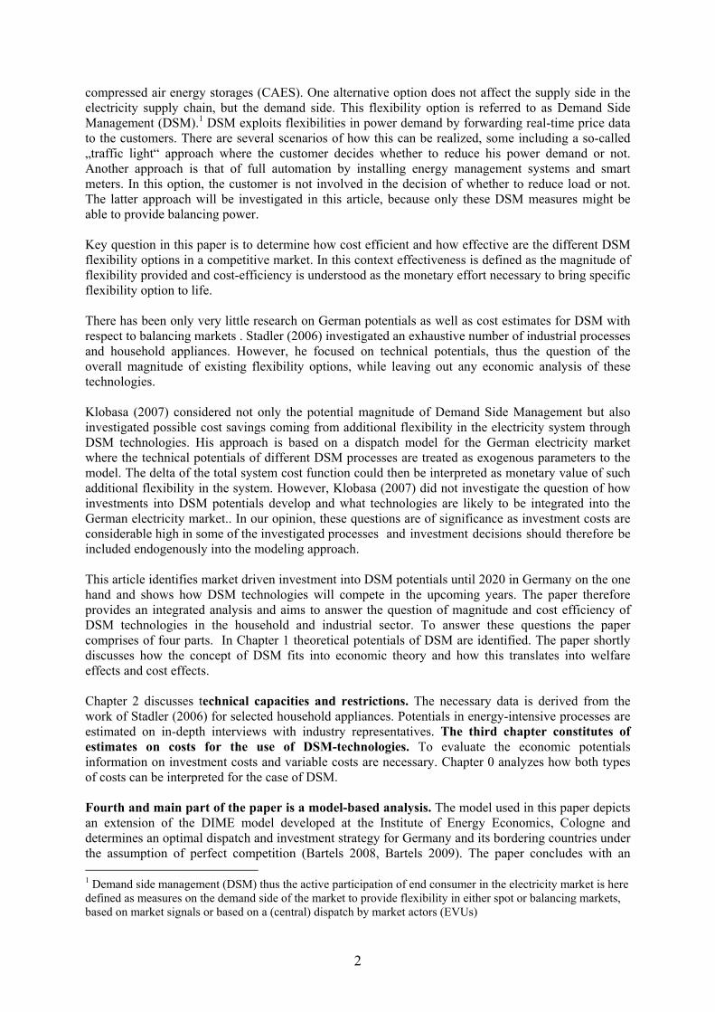
Figure 3: Distribution of rents and welfare changes during off-peak hours with and without DSM (EWI).
The total welfare change by introducing Demand Side Management depends on the number of peak hours hP and off-peak hours hOP with hP + hOP = 8760 (average number of hours per year). Total annual welfare change through introduction of DSM results in:
[ ] [ ]∫∫+
−
−⋅+−⋅=∆DSMOP
OP
p
DSMp
xx
xOP
x
xxPOPPDSM dxxMOxDhdxxDxMOhxxWelfare )()()()(),( .
For xDSM > 0 and xP > xOP the welfare change will always be positive. If xDSM = 0 welfare change will be zero as no load is shifted between high-price and low-price periods due to the fact that load shifting might not be economically attractive or not possible from a technical point of view for the underlying DSM processes. If xP = xOP there exists no price deviation which would make a load shift attractive. The case that xP < xOP is not relevant as this would mean a “reversed” Peak-Offpeak case which would again yield positive welfare change.
2. Demand Side Management potentials in households and energy-intensive industries
Potentials for Demand Side Management arise in a wide range of industries and applications. Power input for industrial processes is often already contracted with a flexible price structure. Typical underlyings for such contracts are spot power exchange prices or fuel prices. It is assumed that household appliances still rely mostly on fixed price power contracts or on contracts which only feature a limited set of prices depending only on the time of day (i.e.: “night-tariffs” and “day tariffs”). A third segment is the trade and commerce sector. All of the three sectors, industry, households as well as trade & commerce feature significant technical potentials for DSM (Stadler, 2006). During the course of the ongoing DENA Netzstudie 2 conducted by EWI and German TSOs for the German grid agency (dena), research focused on the analysis of economically feasible DSM potentials in a number of selected household appliances and energy intensive industries only. This approach tried to capture the most important processes and appliances with the largest technical potential for DSM. The following paragraphs will provide information on the input data later used for the model-based analysis of economically feasible DSM potentials. This input data can be interpreted as technical potentials for Demand Side Management in the investigated industries and processes. The data is based on primary research conducted by the EWI for the energy intensive industries and on research conducted by Stadler (2006) for household appliances.

9
2.1 Classification of industrial sectors Highest economic potential for demand side management in the industrial sector arises from large-scale and energy-intensive processes based on a single source of demand. Contrary to energy intensive industries bundling of small sources of industrial demand becomes a difficult task due to individual characteristics of the underlying processes. Thus significant costs for monitoring and control would arise to integrate these processes into the balancing market. (Borggrefe and Paulus, 2009) The analysis of the industrial sector in this paper focuses on the analysis of large-scale industrial processes for demand side management. Following the approach by Borggrefe and Paulus (2009) processes with high economic potential for DSM are identified within a structured top down analysis. This analysis is based on two criteria “overall potential” as well as “economic efficiency” and is combined with a technical bottom-up analysis for specific processes.
Figure 4: Top down analysis of demand side management potential in balancing markets in Germany (EWI).
Results of the top down approach are depicted in Figure 4. The industrial sector in Germany with an annual electricity demand of 252,6 TWh can be categorized by its branches of industry. From these approximately 250 branches identified by the official statistics2 those sectors are selected and further analyzed with a high electricity demand (Criterion 1) and high specific costs for electricity within each sector. (Criterion 2). For the first criterion the share of electricity consumption in overall industrial electricity demand is used in this analysis as an indicator for overall electricity consumption. This criterion implies that similar processes can be bundled to meet the capacity requirement for bids in the balancing market of 15 MW. The specific costs for electricity in criterion 2 are measured based on electricity costs per gross value added in each sector. This implies that energy intensive industries have a higher willingness to interfere into their production process due to high opportunity costs arising from the potential to sell their DSM potentials into spot and balancing markets. Industry branches with small electricity demand compared to overall production costs, however, are unlikely to disrupt their production process due to small opportunity costs. 2 For more information please refere to www.destatis.de, Fachserie 4 (industry, commerce and trade).

10
To reduce the processes that undergo an bottom-up process by process analysis we only investigate processes with minimum values of 1,5% (Criterium 1: electricity demand) and 5% (Criterium 2: specific electricity costs). Eight branches remain with an electricity consumption of 97 TWh this corresponds to 40% of the overall electricity demand in the industrial sector. Thus the selected industrial branches depict large energy consumers with a high share of electricity costs within their production processes. For each of these industrial branch all important DSM relevant process have been determined based on a detailed bottom-up analysis of its company structure as well as its production processes.3 The analysis identifies especially all processes that have the technical potential to provide DSM and are capable to provide balancing power. All together the analysis identifies a process based DSM potential of 49 TW which corresponds to maximum capacity of 2660 MW that can be used to provide balancing power. The following section describes the relevant processes in more detail.
Industrial processes Chloralkali process The Chloralkali process is an important method for the production of chloride. Chloride is produced via an electrolytic process involving a chloralkali dilution. Chloride production stemming from Chloralkali processes amounted to approximately 5.1 mn. tons in 2005 (DSTATIS, 2009). The two most common processes employed are the so-called Mercury process and the Diaphragm process. Both processes have in common that they are relatively power-intensive and that there exists flexibility in reducing the load for a certain period of time until the temperature of the electrolysis has reached a certain lower threshold temperature. Through personal interviews, we evaluated the flexibility of the chloralkali process and its potential for DSM.
0%10%20%30%40%50%60%70%80%90%
100%
Figure 5: Annual utilization levels of a typical chloralkali producer on a quarter-hourly basis (EWI).
The Chloralkali process is normally executed at full capacity to assure maximum returns of this capital-intensive chemical process. Utilization levels usually range between 80-90%. The load of the Chloralkali process can be reduced by up to 40% for up to 2 hours. Most importantly, the potential to shift load between time periods is severely hampered by the high utilization level which only allows a very slow catch up of load which was shedded. Today, that 40% of capacity (around 660 MW) is already marketed as positive tertiary power reserve capacity. Positive DSM potentials of the Chloralkali process are already fairly exploited. Through the high value of lost load only a minimum number of actual scheduling and physical dispatch occur for positive reserve energy. Positive capacity reserve is already certified and used for demand side 3 For more detail see Borggrefe and Paulus (2009)

11
management in the German electricity market. Negative DSM potentials remain undeveloped but also fairly small. Negative tertiary reserve energy could be marketed in small amounts but also faces very tight storage restrictions. Mechanical wood pulp production The paper industry produces a variety of goods such as different types of cardboard and paper. Main inputs are old paper and pulp. The pulp consists of fibers which are extracted either by a mechanical process or by a chemical process from wood. Primary DSM potentials lies in the mechanical process for pulp production, due to its high energy intensity. When analyzing the production process the main DSM potentials lies in the so-called refiner. These are powered by electric engines with significant power consumption. The refiners can be fully activated or shut down within a few minutes. The only restriction is that the intervals between ramp-up and shutdown do not happen immediately in sequence, due to an excessive wear off of the components. Utilization levels vary but typically lie within a range of 80%. Mechanical wood pulp production was 1.5 mn. tons in 2007 (DSTATIS, 2009). According to our analysis, there exists significant load shifting potential, due to the possibility to store the pulp. This potential can be used either on the spot market or through the positive and negative tertiary reserve markets. Positive DSM potentials are equivalent to the average load of refiners which is 250 MW (80% of 312 MW) and negative DSM potential is defined by the average unutilized capacity of 62 MW (see Figure 6). The current pulp storage volume at most of the paper mills is large enough to accommodate 1.5 hours at maximum capacity, thus giving the process a storage capacity of 468 MWh.
0
50
100
150200
250
300
350
t
MW
Negativepotential
PositivepotentialLoad
Figure 6: Positive potential and negative potential for DSM of the refiner-based wood pulp production
(EWI).
Aluminum electrolysis Aluminum electrolysis converts aluminum oxide through an electrolytic process into aluminum and oxygen. The power demand for activating the electrolysis and bringing the process up to temperature is significant, resulting in an energy intensity of 15 MWh/t of aluminum. Utilization levels ranged from around 95%-98% on an annual basis due to the capital intensiveness of the process. Thus, aluminum electrolysis falls into the category of load shedding as almost no load can be caught up later on. According to the interviews the power demand of the electrolysis can be reduced by up to 25% for up to 4 hours before the process runs into danger of coming to a halt. This 25% or 277 MW is typically already marketed as positive tertiary capacity. The price for actually calling positive reserve energy is high, as the value of lost load is defined by the price of aluminum and technical dangers of destabilizing the electrolytic process (see Figure 7).

12
400
700
1000
1300
60 120 180 240 300MW
€/M
Wh
Figure 7: Merit Order of tertiary positive regulating energy for Aluminum electrolysis in Germany in
2008.
Generally, DSM potentials in this industry are already exploited to a significant extent. This is mostly due to very high intensity energy and thus companies have already marketed their flexibility as positive reserve capacity and observe the spot market for intra-day load reduction or load increase.
Electric arc furnace An energy intensive way of producing steel is by melting scrap steel in an electric arc furnace. In this process, heat is generated by an electric arc or induction which starts the melting of the scrap metal in the furnace. This process can be disrupted immediately. If the disruption takes more than 30 minutes, the scrap metal will cool down and the overall melting process has to begin again. Energy intensity of the process is approximately 0.525 MWh/t of steel produced. Utilization levels are around 75%, as the typical melting process takes 45 minutes to melt the scrap steel and about 15 minutes to empty and refill the furnace. This utilization level cannot be increased due to the aforementioned process. As utilization cannot be increased the DSM potential is strictly load shedding. The company has the flexibility of completely shutting down the process to sell the contracted power on the spot market or on the market for regulating energy. Further extra costs arise if the disruption of the process takes longer than 30 minutes. Currently, approximately 50% of steel mills in Germany have pre-qualified their furnaces in the tertiary reserve market as positive capacity. Capacity prices tend to be fairly moderate, while prices for reserve energy lie beyond 1000 €/MWh due to the high value of lost load in the process.
Cement mills Cement mills crush cement clincer produced in upstream processes and mix it with other ingredients such as hard plaster to generate cement with the desired characteristics. Cement mills constitute the part of cement production with the highest energy intensity. Estimated installed capacity of all cement mills in Germany is 314 MW with an average utilization level of around 80%. These cement mills can be regulated in a flexible way, shutting it down and ramping it up again within minutes. Nevertheless, interviews with industry representatives lead to the conclusion that utilization levels have almost reached technical limits and that storage capacity is a bottleneck for many cement mills. Furthermore, production dependencies with upstream and downstream process parts are a hindering factor in realizing load shifting potential in the cement mills. Therefore, DSM potential in cement mills can only be realized by load shedding. The value of lost load varies widely, as it depends mainly on cement prices.
13
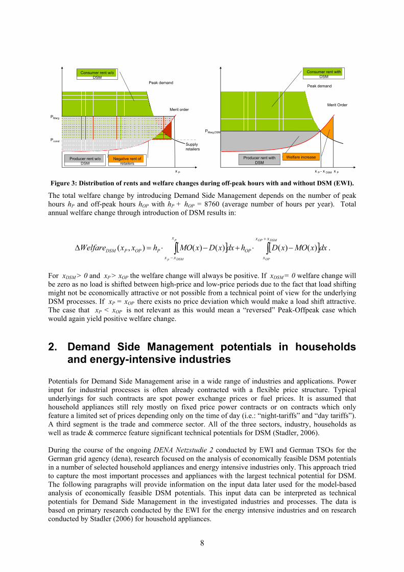
Overview industrial processes Table 1 and Table 2 summarize technical parameters of the investigated energy-intensive industrial processes and classify them either as load shifting potential or as load shedding potential.
Table 1: Overview and scope of the investigated industrial processes (EWI).
Process Relevant elements Technical capacity [MW] Classification
Chloralkali electrolysis Electrolysis 660 Load shifting/shedding Aluminum electrolysis Electrolysis 277 Load shedding Cement mills Milling 314 Load shedding Wood pulp production Mechanical refining 312 Laod shifting Electric arc furnace Melting 1097 Load shedding
Table 2: Overview of technical parameters of the investigated industrial processes.
Process Technical potential [TWh/a]
Storage volume [MWh] Restrictions
Energy intensity [MWh/t]
Chloralkali electrolysis 14.6 1320 Utilization, storage size, process risk 2.85
Aluminum electrolysis 9.7 n/a Utilization, process risk 15
Cement mills Wood pulp production 2.2 468 Medium storage size 1.5
Electric arc furnace 7.2 n/a Utilization, cool-
down, energy intensity
0.53
2.2 Household appliances Total power consumption in German households amounted to 159.5 TWh in 2005 (28.8% of total power consumption in 2005). A small number of appliances constitute around 50% of total power consumption in households:
• Night storage heaters (23 TWh in 2005) • Electrical warm water supply (7 TWh in 2005) • Fridges & Freezers (19 TWh in 2005) • Washing machines, dish washers & tumblers (15 TWh in 2003) • Heating pumps (15TWh in 2005)
Other household appliances like lighting and small-scale electrical devices where not considered in the analysis due to the their low item-specific power consumption or due to technical restrictions.

14
150,14
82,8
16023
7
19
15
15
82,5
161,5
Industry
Craft & trade
Transportation
Night storage heating
El. Warm water
Fridges & freezers
Washing maschines, dish washers& tumblersHeating pumps
Rest households
Figure 8: Overview of power-intensive household appliances (in TWh/a) in comparison to total energy
consumption in Germany in 2005 (DESTATIS).
We will now briefly describe the technical DSM potentials of the investigated load shifting and load shedding processes and appliances in households. Besides capacities usable for DSM, costs of operation and load shifting as well as technical limits to the total shifting volume and other technical descriptions will be discussed. Night storage heating Night heaters were installed during the 60s and 70s in Germany where power generation costs were relatively low due to low fossil fuel prices. The main advantage of night heaters was the smoothing of the daily load curve by charging the heaters only during the night. Today, night heaters are considered to be energy inefficient compared to other modern heating systems and are no longer installed. A law introduced in April 2009 allows banishment of night heaters in Germany starting from 2020 (§4 Abs. 3 EnEG 2009). Night heaters consist of a core which serves as a thermal energy storage. This core is typically made of a material with high specific heat capacity, such as magnesite or other ferric oxides. Total thermal storage volume depends on outside temperature (cf.. Figure 9). During summertime, storage capacities are practically zero to prevent overheating of room temperatures.

15
0%
20%
40%
60%
80%
100%
Spring Summer Autumn Winter
Figure 9: Variable night storage heater capacities for average seasonal temperatures (EWI).
DSM potential of night storage heaters is classified as load shifting potential. Positive DSM potential for night storage heaters is available during periods when the heaters would conventionally generate load, e.g. during the night and early morning hours. During these periods, the heaters could stop charging anytime and thus reduce generated load. Negative DSM potential is available during all hours when the heaters could possibly increase load. This is possible almost anytime, as even during night hours, the heaters generally do not charge at maximum capacity, as outside temperatures rarely reach such that levels which require a charging of heaters at full capacity.
Electric warm water storages in households Electric warm water storages consist of two devices: an heating device for heating water and a storage device in which the warm water can be stored over longer periods of time without significant energy losses. Typical storage volumes range from 5 l to 1000 l (Source Stadler 2006). Only larger warm water storages (more than 30 l in capacity) are suited for Demand Side Management as installation costs of the necessary hardware would be prohibitively high. Warm water storages work very similarly to night storage heaters. One main difference is that their storage is not made of ferrous oxide but water. Water has a comparatively high specific heat capacity, though not as high as that of magnesite. During night hours, the water storage generates load by heating up the stored water. Warm water is consumed during the day hours and, if the storage should prove to be insufficient to serve demand, extra heating occurs during the day. This concept provides a natural thermal storage for DSM and load shifting potentials. Positive DSM potentials are available during night hours, when the warm water supply typically heats up its water storage. During the day, there exists only a very small load shifting potential coming from the occasional daytime warm water heating. Negative DSM potentials are available during any hour when the warm water supply could possibly increase its power demand, e.g. especially during daytime hours. But also at night, capacity of warm water heating is utilized only to a low extent, at least if average numbers for the whole year are considered. Refrigerators and freezers in households The electrical production of cooling works in a similar way to night storage heaters and electrical warm water supplies. Refrigerators and freezers function as a thermal storage but this time in the reverse way by constantly reducing the temperature of their storage contents below outside temperature. The storage contents have an important impact on the size of the storage capacity. The specific heat capacities of different food types differ widely. Air has a lower specific heat capacity than any food. Therefore, the more a refrigerator is filled, the higher its storage capacity. Consistent with night storage heaters and electrical warm water supply, DSM potentials are defined as positive if existing load is shedded- and as negative if load is caught up. A difference with cooling devices is that they typically have to catch up their load in advance, that means cooling down to

16
abnormally low temperatures to be able to shed load later on. Otherwise, food quality could not be assured. Positive and negative DSM potentials are displayed in Figure 10.
0GW
3GW
6GW
9GW
12GW
1 3 5 7 9 11 13 15 17 19 21 23
Figure 10: Positive DSM potentials (blue) and negative DSM potentials (grey) for refrigerators and freezers (EWI).
Tumble dryers, dishwashers and washing machines Tumble dryers, dishwashers and washing machines have in common that they are all non-thermal appliances in contrast to the other appliances investigated so far. These non-thermal appliances can nevertheless be interpreted as a power storage facility with DSM load shifting potential. In contrast to the other appliances, this potential does not stem from managing a thermal storage more efficiently but from altering the consumers’ habits of using these appliances. One important aspect in this context is how severely consumers are restricted by altered using schemes and to what level one must compensate them. The load shifting potential of these appliances lies in altering the time of day at which the respective item is used. E.g.: instead of washing a load of laundry at noon, it could be washed late in the evening. The aggregated load curves scaled to the level of all households in Germany for the year 2003 can be seen in Figure 11.
0
0,5
1
1,5
2
2,5
3
3,5
4
1 2 3 4 5 6 7 8 9 10 11 12 13 14 15 16 17 18 19 20 21 22 23 24
hour
Load
[G
W]
Figure 11: Daily aggregated load curve for non-thermal household appliances in Germany in 2003
(Stadler, 2005).
The load curve in Figure 11 can be interpreted as the positive DSM potential for the investigated non-thermal appliances. The negative DSM potential, the amount by which the appliances can increase their power consumption, is calculated by subtracting the aggregated daily load curve from the calculated installed capacity of 20.8 GW in every hour (Figure 12).

17
0
5
10
15
20
25
1 2 3 4 5 6 7 8 9 10 11 12 13 14 15 16 17 18 19 20 21 22 23 24
hours
Cap
acit
y [
GW
]
Figure 12: Negative DSM potential for non-thermal household appliances in Germany in 2003 (Stadler,
2005).
Heating pumps Heating pumps are used to distribute the heat produced in the boiler to the radiator where it is dispensed into the room. Heating pumps are generally significantly oversized. Furthermore, their use becomes more inefficient if outside temperatures reach a certain band. For a more detailed description, see Stadler (2005). Heating pumps feature no load shifting potential but load shedding potential only. This potential stems from deactivating the heating pump during time periods with moderate outside temperatures until room temperatures have reached a certain lower threshold when the heating pump comes into action again. This positive DSM potential is dependent on outside temperatures and on the time span since the heating pump was deactivated (a function of the insulation of the respective buildings). A graph of this DSM load shedding potential can be seen in Fehler! Verweisquelle konnte nicht gefunden werden..
120
39
58
-12 -8 -4 0 4 8
12 16 20
0
0,5
1
1,5
2
2,5
Posi
tive
DSM
pot
entia
l [G
W]
duration of discharge [h]
Outside temperature [°C] Figure 13: Positive DSM load shedding potential for heating pumps in Germany (Stadler, 2005).
Overview household appliances Table 3 and Table 4 depict aggregated information on technical restrictions, parameters and potentials of the investigated household appliances.

18
Table 3: Overview of household appliances and their classification (EWI).
Appliance Type Technical capacity [GW] Classification
Night storage heating Thermal storage 34.9 Load shifting El. warm water supply Thermal storage 5.7 Load shifting Fridges & freezers Thermal storage 10.6 Load shifting Washing machines, dish washers & tumblers
Storage through change of usage pattern 20.8 Load shifting
Heating pumps Efficiency increase 2.2 Load shedding
Table 4: Overview of household appliances and their technical parametwers (EWI).
Appliance Technical potential [TWh/a]
Storage volume [GWh] Restrictions Specific size
[W]
Night storage heating 23 185.0
Storage volume dependent on temperature
14000
El. warm water supply 7 44.4
Positive potential only during night
time 1400
Fridges & freezers 19 29.0 Low specific storage volumes 300
Washing machines, dish washers & tumblers 15 41.6
Short storage times, consumer utility
reduced 730
Heating pumps
15 n/a
Low specific capacities, potentials dependent on outside
temperature
25
2.3 Costs for accessing DSM potentials There are three types of costs relevant for accessing and using DSM potentials: investment costs for installing the necessary smart metering equipment, variable costs to account for the value of lost load and fixed costs mainly depending on data exchange between the single DSM units and a central control center which pools the DSM units into larger chunks of capacity. Investment costs are especially relevant for household appliances. They cover costs for the smart meter, cost for software and maintenance of the control center, costs of the energy management system and costs for the data exchange unit. The energy management system is attached to each single DSM unit and allows an automated control of the power demand of that unit.
19
1
10
100
1000
10000
2010 2015 2020
€/K
W
Night heaters & warm waterFreezers & FridgesTumblers, washing maschines & dryersHeating Pumps
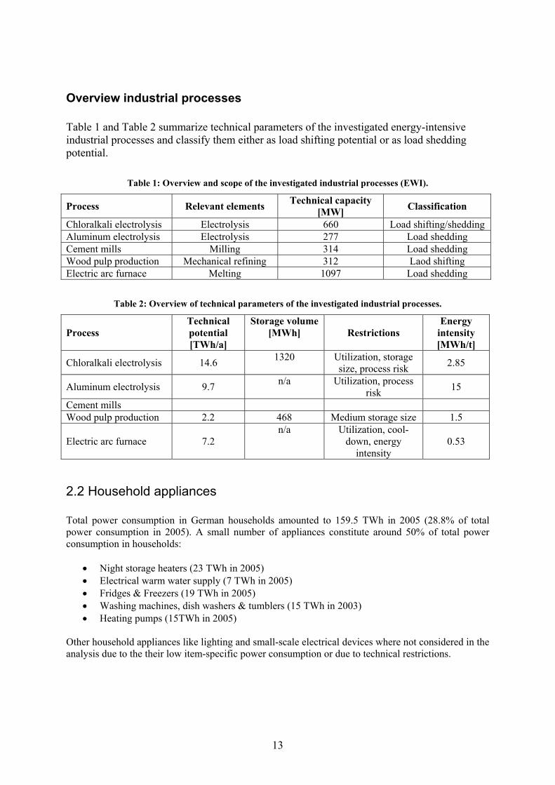
Figure 14: Investment costs in €/KW for household appliances in Germany until 2020 (EWI).
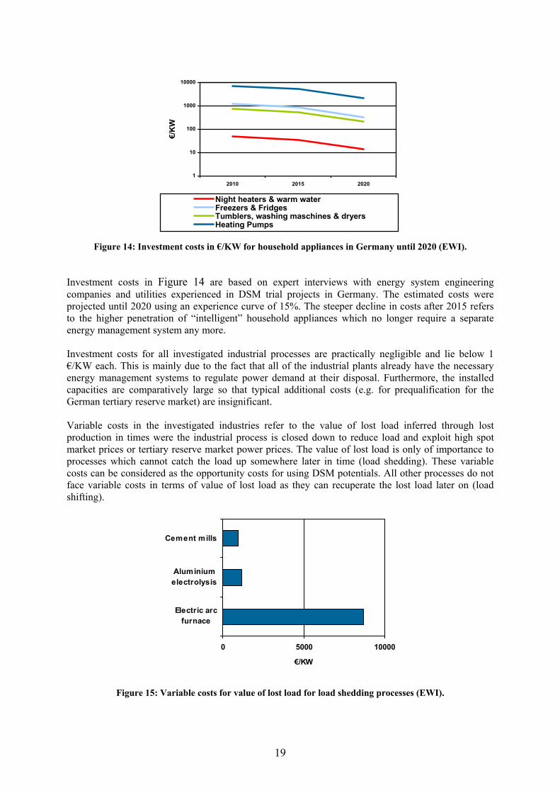
Investment costs in Figure 14 are based on expert interviews with energy system engineering companies and utilities experienced in DSM trial projects in Germany. The estimated costs were projected until 2020 using an experience curve of 15%. The steeper decline in costs after 2015 refers to the higher penetration of “intelligent” household appliances which no longer require a separate energy management system any more. Investment costs for all investigated industrial processes are practically negligible and lie below 1 €/KW each. This is mainly due to the fact that all of the industrial plants already have the necessary energy management systems to regulate power demand at their disposal. Furthermore, the installed capacities are comparatively large so that typical additional costs (e.g. for prequalification for the German tertiary reserve market) are insignificant. Variable costs in the investigated industries refer to the value of lost load inferred through lost production in times were the industrial process is closed down to reduce load and exploit high spot market prices or tertiary reserve market power prices. The value of lost load is only of importance to processes which cannot catch the load up somewhere later in time (load shedding). These variable costs can be considered as the opportunity costs for using DSM potentials. All other processes do not face variable costs in terms of value of lost load as they can recuperate the lost load later on (load shifting).
0 5000 10000
Electric arcfurnace
Aluminiumelectrolysis
Cement mills
€/KW
Figure 15: Variable costs for value of lost load for load shedding processes (EWI).

20
Figure 15 shows the variable costs for the three investigated load shedding processes. Note that variable costs of the electric arc furnace are far higher than for example for aluminum electrolysis as the energy intensity of the steel production process is significantly lower (0.525 MWh/t) compared to aluminum electrolysis (15 MWh/t). Industrial processes which can be classified as load shifting processes have practically no variable costs. Household appliances have no strictly variable costs in general as no household compensation for participating in the DSM scheme was considered. Fixed costs for accessing DSM potentials stem from the data connection between the smart meter and the energy management system of each appliance on the one hand, and between the smart meter and the control center on the other. It was assumed that roughly 90% of all households would use DSL technology for the data exchange due to its broad availability and cost efficiency. The other 10% of households would use the cellular phone network for communication in the case that no DSL technology is available.
Night heaters & w arm w ater
Freezers & Fridges
Tumb-lers, w ashing maschi-nes, dish w ashers
Heating pumps
€/KWa
10€/KWa
20€/KWa
30€/KWa
40€/KWa
50€/KWa
2€/KWa
41€/KWa
33€/KWa
45€/KWa
Figure 16: Fixed costs for data exchange for household appliances in Germany (EWI).
Figure 16 shows fixed cost assumptions for the household appliances. Note that these indivisible costs for communication advocate the appliances where larger potentials can be accessed, such as night storage heaters. The investigated industrial processes have negligible fixed costs as communication links between their plants and control centers are typically already installed. Even in the case of no installed communication technology, the fixed costs would be insignificant because of the size of DSM potential typically available in each plant.
3. Modeling investments into Demand Side Management potentials
The question of what the market driven investment into DSM potentials could be can only be answered consistently if the interdependencies between DSM potentials, power plant fleet, aggregated demand and increasing volatile renewable energy feed-in is respected. The electricity market model employed by us is DIME (Dispatch and Investment Model for Electricity Markets in Europe). DIME was developed to combine the advantages of earlier simulation tools of the Institute of Energy Economics, namely GEMS (German Electricity Market Simulation) and CEEM (Cogeneration in European Electricity Markets). At the same time, the regional coverage of the earlier models was extended. DIME is designed for long term forecasting. The model is formulated as a linear optimization model for the European electricity generation market. It is applied to simulate dispatch as well as investment decisions regarding the supply side of the electricity sector. The objective function minimizes total discounted costs based on the assumption of a competitive generation market.

21
In our model, 12 countries, mainly located in Western and Central Europe as well as the Danish UCTE area (Denmark West), are represented in the model. For further description of DIME, see Bartels (2008). For a detailed overview of the DSM-specific model enhancement necessary please refer to Appendix A on page 26.
4. Scenario runs Scenario runs were conducted with the enhanced DIME model to investigate endogenous investments in DSM. The model horizon covered reference years from 2007 to 2040. However, only results up to 2020 will be analyzed due to decreasing robustness of results. The DIME model was parameterized with assumptions to be found in the forthcoming dena2 Netzstudie (DENA 2010). Main assumptions especially important for the endogenous investment in DSM potentials are the feed-in of renewable energy sources and fossil fuel prices (Figure 17 and Figure 18).
0
10
20
30
40
50
60
2008 2010 2015 2020
€/M
Wh(
th)
Hard coal Lignite Natural gas Oil
Figure 17: Cost assumptions of fossil fuels for scenario runs (EWI).
Further parameters used in the DIME model include assumptions on CO2 prices, power plant investment costs, ramp-up costs of power plants as well as assumptions on cogeneration levels up to the year 2040. All assumptions will be published in the forthcoming dena2 Netzstudie (DENA 2010). A short summary of the main model results for DIME can be found in the appendix on page 30.
30%
23%
15%12%40
80
120
2007 2010 2015 2020
TWh
0%
10%
20%
30%
40%
Others Wind Ratio RE
Figure 18: Assumptions on renewable energy feed-in until 2020 in Germany (EWI).

22
4.1 Results Already installed DSM capacity of the investigated industrial processes amounted to approximately 1500 MW in 2007 (c.f. Figure 19). All untapped DSM potential is made accessible until 2010. Afterwards, DSM capacities remain almost constant, except for small reductions due to overall production reduction of these industries in Germany. The rapid exploitation of remaining DSM potential in the energy intensive industries seems reasonable, as investment costs for accessing these potentials is negligible. Especially of interest here is that until 2008 neither wood pulp producers nor cement mill owners had been active in marketing their processes on tertiary reserve markets or spot power markets. Reasons therefore could lie in the relatively dispersed structure of these industries, especially of the wood pulp industry, which could hinder the development of such specialized services. Technical restrictions do not seem to be very probable reasons, as our expert interviews with industry representatives should have let such restrictions come to surface.
667 667 643 618
312 312 312277277 277 277549
1098 1098 1098
314 347 383
0
500
1000
1500
2000
2500
3000
2007 2010 2015 2020
MW
Chloralkali electrolysis Wood pulp production
Aluminium electrolysis Electric arc furnace
Cement mills
Figure 19: Endogenous DSM capacity development for energy-intensive industries in Germany until 2020 (EWI).
The situation for household appliances is different, as Figure 20 shows. Only night storage heater potential and heat pumps potential is made accessible until 2020. This outcome is not only due to the high investment costs for tapping the household potentials (The heat pumps have by far the highest investment costs with more than 7000 €/KWh), but also due to technical constraints which are in some cases severely limiting. Washing machines, dryers and dish washers can only offer their load shifting potentials for short periods (24 hours) before they have to catch up load again. Freezers and refrigerators are more flexible with regard to the time span of load shifting, but do suffer from moderately large specific capacities for shifting electricity demand. One important aspect is also the underlying assumptions regarding the learning curve inferred investment cost reductions. Model outputs are quite sensitive to these assumptions (currently, doubling the number of smart metering devices reduces unit costs by 15%). The model results for 2025, for example, show significantly higher investments in household appliances, also in refrigerators and freezers.

23
173
36
36
0
10
20
30
40
50
60
2007 2010 2015 2020
MW
Heating pumps Night storages & warm water
Figure 20: Endogenous DSM capacity development for households in Germany until 2020 (EWI).
While significant DSM capacities are available in energy-intensive industries from 2010 onwards, Figure 19 and Figure 20 do not give any information about how often these capacities are called upon, i.e. how much load is shedded or shifted. As seen in chapter 2, several energy-intensive processes face significant high price levels for their value of lost load. This high opportunity costs should limit the actual load reduction of these „expensive“ DSM capacities to several rare hours of high price peaks or inhibit them completely. Table 5: Load reductions and load catch-ups for all DSM processes and appliances available in Germany
in 2020 (EWI).
Process Load reduction [GWh] Load catch-up [GWh]
Spot Reserve Spot Reserve
Night storage heaters 12.3 1.8 5.6 8.6
Chloralkali-process 11.4 0.0 0.0 11.4
Wood pulp production 232.1 0.0 33.4 198.7
Heat pumps 99.3 0.0 0.0 0.0 As can be seen in Table 5, the only significant load shifting takes place in wood pulp production. This process has very low opportunity costs, due to its capability to catch-up load and because of the high flexibility with which it can be handled. Note that all processes which can only engage in load shedding (aluminum electrolysis, electric arc furnace and cement mills) do not reduce load in any hour of the year 2020. The Chloralkali process has the ability to catch up lost load later on and therefore avoid the high opportunity costs for lost load. Nevertheless, technical restrictions such as storage volumes and other production processes along the supply chain in which this process is embedded, prevent any significant load reduction in 2020. Load reduction and load catch-ups in Table 5 refer to tertiary reserve energy markets and spot power markets. On the other hand, the DSM capacities developed in energy intensive industries do supply capacity to the capacity reserve markets. Table 6 shows the positive capacities and negative capacities which are marketed as tertiary reserve capacity in DIME. All together, the DSM processes and appliances will amount to 60% of total necessary tertiary reserve capacity in 2020. This represents a significant impact of DSM on the markets, as it will reduce the requirement to built new conventional (gas-fired) power plants which typically supply reserve capacity.

24
Table 6: Positive and negative tertiary reserve capacity for all DSM processes and appliances available in Germany in 2020 (EWI).
Process Ø Positive capacity offered [MW]
Call prob. [%]
Ø Negative capacity offered [MW]
Call prob. [%]
Night storage heaters 0.2 98.9 20.3 4.8
Chloralkali-process 616.3 0.0 8.0 16.2
Wood pulp production 119.6 0.0 24.2 93.9
Aluminum electrolysis 166.8 0.0 0.0 0
Electric arc furnace 684.5 0.0 0.0 0
Cement mills 204.0 0.0 0.0 0 The amount of positive reserve capacity supply is significantly higher than the amount of negative capacity, as most of the processes already operate on high utilization levels which limit the amount of supplied negative reserve capacity. One can argue that it should not be possible in reality to decouple the supply of capacity and the supply of actual energy in this particular way. Any offer of reserve capacity yields a possibility of also having to supply reserve energy depending on the reserve energy price offered. While this holds true and shows a weakness of the deterministic model used, it can also be interpreted from an economical point of view: Owners of the industrial plants offer reserve capacities for moderate prices on the tertiary reserve markets. Their offered reserve energy prices are very high, mirroring their value of lost load and thus reduce chances of being called on for reserve energy. Actually, this strategy is already used by several companies operating the Chloralkali process. As previously mentioned, cost savings are generated by the substantial amount of positive tertiary reserve capacity administered by energy intensive industries. To a smaller extent, the load shifting also generates cost reductions. Figure 21 shows a split-up of cumulated system cost savings (million €, discounted to 2007). Total system cost savings amount to 481 mn. € up to 2020. This cost reduction corresponds to 0.36 % of the total cumulated power market system costs in Germany up to 2020. Major cost savings are generated by reduction of investment costs. These costs translate into the avoided investments for gas turbines which often supply the tertiary positive capacity. In terms of model investments the saved investment costs correspond to roughly 800 MW of gas turbine capacity. Other cost savings are relatively minor and come mostly from reduced power demand during peak hours, which reduce the net import during these periods. Reserve energy cost savings refer to the average reserve energy prices which are lowered by the introduction of DSM. Welfare change can be calculated on the basis of cost savings generated by load shifting only. Load shedding generates no welfare increase as cost reductions equal generated welfare if load is shedded. Total welfare increase amounts to 474 mn € up to the year 2020.

25
342
481
0-2 64032
-18
63
0
100
200
300
400
500
600
Total Reserveenergy
Grid Production Ramp-up Part-load IM-EX FO&M Investment
Mio
. € [2
007]
∆Costs: -0,3% -4,1% +0,1% 0,0% 0% 0% -0,7% -0,4% -2,3% Figure 21: Split-up of cumulated cost savings generated by introduction of DSM in selected industries and
appliances in Germany up to 2020 (EWI).
5. Conclusions We discovered that the main market for an economic usage of DSM potentials of the selected industrial processes and household appliances will be the tertiary capacity reserve market up to the year 2020. The reason therefore lies in the cost structure of the industry and household DSM potentials. Energy-intensive processes have only negligible investments for accessing their DSM potentials but have high opportunity costs due to the value of lost load in the case that they cannot recover their load later on. On the other side, household appliances have significant investment costs due to the costly smart metering equipment and energy management systems. Opportunity costs for household appliances are negligible, as the services provided by such appliances are not constrained in any (observable) way. The conducted analysis faces two main sensitive parameters: the calculation of the value of lost load for energy intensive industries and the investment cost assumptions for household appliances. Both parameters are not easily surveyed and are therefore prone to significant estimation errors. The focus of further research will continue to be obtaining robust estimates for the aforementioned parameters. A possible next step could be to develop a standardized method for estimating the value of lost load in different industries. The estimates of this method could be compared to the interview-based estimates used so far. Furthermore, the focus of the analysis could also be broadened to cover other relevant processes like industrial cooling, as well as an analysis of processes in the commerce and trade sector.

26
6. Appendix A DIME can be described as:
( ) ( ) ( ) ( )
( )00:
≥∀≤
xixf
s.t.xRC+xIC+xFC+xVC=zmin
i
x Decision vector
VC Variable costs of production
FC Fixed costs
IC Investment costs
RC Costs for reserve energy and capacity
fi Linear constraint i
z Total electricity market system costs DSM potentials were modeled by interpreting load shifting processes as power storages and load shedding processes as virtual power plants. The temporal dimension in the model is broken down into years y, seasons s, days d and hours t. Processes were modeled by introducing new linear constraints to the model. All DSM load shedding processes j have to fulfill the capacity criterion. This means that the sum of spot market shedding and reserve capacity supply has to be lower or equal than initially installed capacity of the process plus investments which happened in the meantime:
∑ −=≤
∀DSM
aj,ya
DSMj
pDSM,ys,t,j,
DSMys,t,j, Inv+Caprc+x
yt,s,j,12008
.
x j ,t , s , y
DSM DSM spot market load reduction by process j in hour t, season s and year y.
r j , t , s , yDSM , p
DSM positive tertiary reserve energy of process j in hour t in season s and year y.
rc j , t , s , yDSM , p
DSM positive tertiary reserve capacity by process j in hour t, season s and year y.
Cap jDSM
Maximum positive DSM potential in starting year.
Inv j , aDSM
Investment in positive DSM potential in year a.
Furthermore, all load shedding processes face a maximum load shedding potential per season, due to technical constrains (e.g: the cooling down of the electrolysis in the case of Aluminum):
( ) ( )∑∑ −=⋅≤
∀DSM
aj,ya
DSMj
DSMys,t,j,
DSMys,t,j,t Inv+Capar+x
yj,s,12008
.
a Technical factor representing the maximum amount of load shedded by process j

27
Load shifting processes are modeled similarly to pump storage facilities. Inflows and outflows for each load shifting process k are modeled through a storage equation. The storage volume for the next hour is defined as storage level of the previous hour plus any spot market load increases and negative reserve energy minus spot market load reductions and positive reserve energy. Furthermore, the actual real demand of the process is subtracted in every hour (e.g.: for night storage heaters the actual demand for power to generate the necessary heating in the respective hour).
actualys,t,k,
pDSM,ys,t,k,
pDSM,ys,t,k,
nDSM,ys,t,k,
nDSM,ys,t,k,
DSMys,t,k,
DSMys,+tk, Demandrxr+x+sto=sto
ys,t,k,−−−
∀
1,
.
stok ,t , s , y
DSM Amount of load shifting potential available of process k in hour t in season s in year y
xk ,t , s , yDSM , n
DSM spot market load increase
r k ,t , s , yDSM , n
DSM negative tertiary reserve energy
xk ,t , s , yDSM , p
DSM spot market load reduction
r k ,t , s , yDSM , p
DSM positive tertiary reserve energy
Demandk ,t , s , yactual
Actual real demand of process k
Load shifting processes face a storage limit. This limit is a multiple of the installed capacity of the process. The multiple can be time variant, depending on the process, e.g. the parameter is zero for night storage heaters during summertime.
( )∑ −=⋅≤
∀DSM
aj,ya
DSMjystk
DSMys,+tk, Inv+CaperStoParametsto
yt,s,k,12008,,,1,
ystkerStoParamet ,,,
Storage parameter defining the storage volume of process k in hour t, season s and year y.
Certain load shifting processes h face restrictions on how long they can store load. For example, wood pulp is only storable for about a week before it starts to deteriorate. Night storage heaters cannot store heat in autumn for the next spring as this would mean significant energy losses and overstress for the heater cores. Therefore, a restriction has to satisfy that storage inflows and outflows sum up to zero for certain time intervals:
actualys,b,k,
pDSM,ys,b,k,
pDSM,ys,b,k,
nDSM,ys,b,k,
nDSM,ys,b,k,
tctb Demandrxr+x=
ys,th,−−−
∀
∑ −=0,
c Maximum storage duration in hours of process h in hour t, season s and year y.
Maximum inflow capacity is similar defined as for load shedding processes:
∑ −=+≤
∀DSM
ak,ya
DSMk
nDSM,ys,t,k,
nDSM,ys,t,k, InvCaprc+x
ys,t,k,12008

28
rck ,t , s , yDSM , n
DSM negative tertiary reserve capacity by process k in hour t, season s and year y.
Furthermore, positive spot market load reductions and positive reserve energy are restricted by the reference case with no DSM potential used. This means that there can be no more positive DSM potential than there was been load formerly:
noDSMys,t,k,
pDSM,ys,t,k,
pDSM,ys,t,k, Demandrc+x
ys,t,k,≤
∀
rck ,t , s , y
DSM , p DSM positive tertiary reserve capacity by process k in hour t, season s and year y.
Demandk ,t , s , ynoDSM
Reference demand of process k in hour t, seasons and year y without DSM
The model constraint for the power balance changes. Spot market load reductions and spot market load increases for DSM have to be incorporated. For load shedding processes, only the delta between spot market load increases and actual real demand of the process have to be respected to avoid double counting:
( ) ys,t,actual
ys,t,k,nDSM,
ys,t,k,knDSM,
ys,t,j,jpDSM,
ys,t,k,kpDSM,
ys,t,j,jys,t, AggDemand+Demandx+x=x+x+ionAggProductyt,s,
∑∑∑∑ −
∀
AggProductiont ,s , y Aggregated conventional production of power plants and storages in hour t, season s and year y
AggDemandt , s , y Aggregated conventional demand and power storage inflows in hour t, season s and year y
The constraints which secure that reserve energy is supplied have to be updated. Positive and negative reserve energy demand can now also be satisfied via DSM processes:
pys,t,
pDSM,ys,t,k,k
pDSM,ys,t,j,j
pys,t, Othersr+r=ResEn +∑∑
n
ys,t,nDSM,
ys,t,k,knDSM,
ys,t,j,jn
ys,t, Othersr+r=ResEn +∑∑ .
ResEnt , s , yp
Positive tertiary reserve energy demand in hour t, seasons and year y
ResEnt , s , yn
Negative tertiary reserve energy demand in hour t, seasons and year y
Otherst , s , yp
Conventional positive tertiary reserve energy suppliers like part-loaded power plants and pump storages
Otherst , s , yn
Conventional negative tertiary reserve energy suppliers like part-loaded power plants and pump storages
Similar restrictions have to be changed for reserve capacities:
pys,t,
pDSM,ys,t,k,k
pDSM,ys,t,j,j
pys,t, OtherCaprc+rc=ResCap +∑∑

29
nys,t,
nDSM,ys,t,k,k
nDSM,ys,t,j,j
nys,t, OtherCaprc+rc=ResCap +∑∑
ResCapt , s , y
p Positive tertiary reserve capacity demand in hour t, season s and year y
ResCapt , s , yn
Negative tertiary reserve capacity demand in hour t, season s and year y
OtherCapt , s , yp
Conventional positive tertiary reserve capacity suppliers like part-loaded power plants and pump storages
OtherCapt , s , yn
Conventional negative tertiary reserve capacity suppliers like part-loaded power plants and pump storages
Lastly, the objective function components for variable costs, fixed costs and investment costs have to include costs of the DSM processes and appliances:
yDSM
yk,inv
yk,kDSM
yj,inv
yj,jy ConInv+InvcInvc=IC ⋅+⋅ ∑∑ ,
( ) ( ) ( )( ) y
nDSM,ys,t,k,
nDSM,ys,t,k,
nvar,yk,stk
pDSM,ys,t,k,
pDSM,ys,t,k,
pvar,yk,stk
nDSM,ys,t,j,
nDSM,ys,t,j,
nvar,yj,stj
pDSM,ys,t,j,
pDSM,ys,t,j,
pvar,yj,stjy
ConVar+r+xc+
r+xc+r+xc+r+xc=VC
⋅
⋅⋅⋅
∑∑∑∑
,,
,,,,,, ,
and ( ) ( ) y
fixyk,
DSMak,
yak
fixyj,
DSMaj,
yajy ConFix+cInv+Cap+cInv+Cap=FC ⋅⋅ ∑∑ −
=−=
12008
12008 .
c j , y
inv Investment costs for load shedding process j in year y
ck , yinv
Investment costs for load shifting process k in year y
ConInv y Investment costs of conventional plants in year y
c j , yvar , p
Variable costs for positive DSM potential of load shedding process j in year y
c j , yvar , n
Variable costs for negative DSM potential of load shedding process j in year y
ck , yvar , p
Variable costs for positive DSM potential of load shifting process k in year y
ck , yvar , n
Variable costs for negative DSM potential of load shifting process k in year y
ConVar y Variable production costs of conventional plants in year y
c j , yfix
Fixed costs for load shedding process j in year y
ck , yfix
Fixed costs for load shifting process k in year y
ConFix y Fixed costs of conventional plants in year y

30
7. Appendix B
0
20
40
60
80
100
120
2007 2010 2015 2020
GW
hardcoal lignite gas nuclear hydro CAES DSM
Figure 22: DIME results for installed conventional power plant fleet and DSM capacities until 2020 (EWI).
40
50
60
70
2007 2010 2015 2020
€/M
Wh
Figure 23: DIME results for base load prices for Germany until 2020 (EWI).

31
-100
0
100
200
300
400
500
600
2007 2010 2015 2020
TWh
Im-ExRenewableshydronuclear
gaslignitehardcoal
Figure 24: DIME results for power generation unitl 2020 (EWI).
32
References Auer H., Huber C., Faber T., Resch G. 2006. Economics of Large-scale Intermittent RES-E Integration into the European Grids: Analyses based on the Simulation Software GreenNet. International Journal of Global Energy Issues, Vol. 25, no. 3: 219-242. Bartels M., Gatzen C., Peek M., Schulz W. 2006. Planning of the grid integration of wind energy in Germany onshore and offshore up to the year 2020. International Journal of Global Energy Issues, Vol. 25, no. 3: 257-275. Bartels M., Lindenberger D. 2008. Systemanalyse und Szenariorechnung. Schwerpunkte und Effizienzstrategien in der Energieforschung, final report, AGFW. Bartels M. 2009. Cost efficient expansion of district heat networks in Germany. PhD diss., University of Cologne. Benston A. editor. 2008. Implementing Agreement on Demand-Side Management Technologies and Programmes – Annual Report 2007, IEA Demand- Side Management Programme. Borggrefe F., Paulus M. 2009. Integrating renewable energies – Long term technical and economic potential for demand side management from energy intensive industries in spot and balancing electricity markets. Forthcoming 5th Dubrovnik Conference on Sustainable Development of Energy Water and Environment Systems. October 2009, Dubrovnik, Croatia. Brückel O., Neubarth J., Wagner U. 2006. Regel- und Reserveleistungsbedarf eines Übertragungsnetzbetreibers Energiewirtschaftliche Tagesfragen 56 (1/2): 50-55. DSTATIS, 2007. Produierendes Gewerbe – Produktion im Produzierenden Gewerbe. Fachserie 4 Reihe 3.1. Statistisches Bundesamt. GDA, 2009. German Aluminium Industry Association on Production Figures for Germany, http://www.aluinfo.de/index.php/produktion.html, 05.08.2009. Geiger B., Hardi M., Brückl O., Roth H., Tzscheutschler P. 2005. CO2 – Vermeidungskosten im Kraftwerksbereich, bei den erneuerbaren Energien sowie bei nachfrageseitigen Energieeffizienzmaßnahmen. Herrsching: Energie & Management Verlag. Klobasa M. 2007. Dynamische Simulation eines Lastmanagements und Integration von Windenergie in ein Elektrizitätsnetz auf Landesebene unter regelungstechnischen und Kostengesichtspunkten. PhD diss., ETH Zürich. Stadler I. 2006. Demand Response: Nichtelektrische Speicher für Elektrizitätsversorgungssysteme mit hohem Anteil erneuerbarer Energien. Berlin: dissertation.de. WV Stahl, 2005. German Economic Association for Steel on Production Figures for Germany. http://www.stahlonline.de/wirtschaft_und_politik/stahl_in_zahlen/start.asp?-highmain=4&highsub=0&highsubsub=0, 05.08.2009.