Embed Size (px)
Citation preview

ECONOMIC PERSPECTIVE OF FARMERS INDEBTEDNESS IN SUICIDAL PRONE
AREA – PUNJAB, INDIA
by
VINAY JAYAPPA
B.Sc., University of Agricultural Science, 2006
A THESIS
submitted in partial fulfillment of the requirements for the degree
MASTER OF SCIENCE
Department of Agricultural Economics
College of Agriculture
KANSAS STATE UNIVERSITY
Manhattan, Kansas
2010
Approved by:
Major Professor
Dr. Allen M. Featherstone

Copyright
VINAY JAYAPPA
2010

Abstract
The number of farmer suicides has been high in Andhra Pradesh, Karnataka,
Kerala, Maharashtra, and Punjab since 2000. Farmers‟ suicide in India is reported to be
due to the burden of debt. While it makes some sense to attribute farmer suicides in
Kerala, Karnataka, Maharashtra, and Andhra Pradesh to indebtedness in view of the
widespread poverty, it is more difficult to consider in the context of the Punjab which is
known for its prosperity.
Others have found that the prime cause for farmer suicides is indebtedness. The
purpose of this research focuses on identifying and quantifying the reasons for farmers‟
indebtedness compared to non-indebted farmers in the same region. This was achieved by
documenting the socio-economic profile of the farmers; studying the extent of
indebtedness and pattern of capital use by farmers, and evaluating the farm business
performance.
Results obtained for the socio-economic profile of the farmer indicated that age,
education, family size and landholding had a significant effect on the probability of a
farmer being indebted. Family size had the largest effect on the probability of indebtness.
A study on the extent of indebtedness and pattern of capital use showed that farmers
depend on non-institutional loans for meeting their financial needs and some loans are
used for non-agricultural purposes. Farm business performance of the sample respondents
showed that they had a negative balance on farm business performance. Some of the
methods to improve the situation would to improve and expand free and compulsory
primary education, thereby reducing the debt incurred on education; diversifying towards
high value/more remunerative crops, reviewing the system of subsidization of

agricultural inputs, and expanding institutional sectors for providing loans at reasonable
interest rates.

v
Table of Contents
List of Figures ..............................................................................................................vii
List of Tables ............................................................................................................. viii
Acknowledgements ....................................................................................................... ix
Dedication ..................................................................................................................... xi
CHAPTER 1: Introduction ........................................................................................... 1
1.1 Farmer Suicides Worldwide ...................................................................................1
1.2 Indebtedness - the prime culprit for farmers‟ suicides? ...........................................3
1.3 Study Objective .....................................................................................................4
1.4 Organization of Study ............................................................................................5
CHAPTER 2: Review of Literature .............................................................................. 6
2.1 Indebtedness of farmers .........................................................................................6
2.2 Extent and pattern of indebtedness of farmers to private and public financial
institution ................................................................................................................9
CHAPTER 3: Methodology ........................................................................................ 11
3.1 Description of the study area ................................................................................ 11
3.2 Sampling procedure ............................................................................................. 26
3.3 Data ..................................................................................................................... 27
3.4 Analytical techniques employed ........................................................................... 27
3.4.1 Tabular analysis – Ratio‟s, percentages ......................................................... 27
3.4.2 T-test ............................................................................................................. 27
3.4.3 Farm Business Analysis Tool ........................................................................ 28
3.4.4 Debt-Equity Ratio (Leverage)........................................................................ 28
3.4.5 Debt Asset Ratio (DAR) ................................................................................ 28
3.4.6 Net Worth ..................................................................................................... 29
3.4.7 Net Capital Ratio ........................................................................................... 29
3.4.8 Logistic Regression Model ............................................................................ 29
3.4.9 Tobit Model .................................................................................................. 31
3.4.10 Tobit model for censored observations ........................................................ 31
3.4.11 Expected Values for Tobit Model (Decomposition) ..................................... 32
vi
3.4.12 Estimation with Heckman‟s Two-Step Procedure ........................................ 33
CHAPTER 4: Results .................................................................................................. 36
4.1 Socio-Economic Profile of the Sample Respondents ............................................ 36
4.1.1 Age ............................................................................................................... 36
4.1.2 Education Level ............................................................................................ 36
4.1.3 Family size .................................................................................................... 39
4.1.4 Land Holding ................................................................................................ 39
4.1.5 Occupational pattern...................................................................................... 39
4.1.6 Distribution of indebtedness by retrospectively reconstructed reasons ........... 41
4.2 Farm Business Performance ................................................................................. 43
4.2.1 Cropping patterns of Indebted and Non-indebted farmers .............................. 43
4.2.2 Cost-return Profile of Major Crops Grown by the Respondents (Rs. /hectares)45
4.2.3 Farm financial ratios ...................................................................................... 47
4.2.4 Asset Position of Sample Respondents .......................................................... 48
4.3 Extent of Indebtedness and Pattern of Capital Use ............................................... 50
4.3.1 Interest Rates ................................................................................................. 50
4.3.2 Liability position of Indebted and Non-indebted farmers in the beginning of
the year .............................................................................................................. 51
4.3.2 Overdue position of the indebted and non-indebted farmers ........................... 55
4.3.3 Sources and pattern of capital use by indebted and non-indebted farmers ...... 57
4.3.4 Logit Estimation Results ............................................................................... 60
4.3.5 Tobit estimation results ................................................................................. 65
4.3.6 McDonald and Moffitt Decomposition .......................................................... 66
4.3.7 Estimation results for Probit and Heckman‟s Two-Step method..................... 68
CHAPTER 5: Summary and Conclusion ................................................................... 72
CHAPTER 6: Policy Implications .............................................................................. 79
References .................................................................................................................... 81

vii
List of Figures
Figure 3.1 Location of the Study Area within India ........................................................ 11
Figure 3.2 Location of the Study Area within the Punjab State....................................... 12
Figure 4.1: Social Characteristics of Indebted Farmers- Age .......................................... 38
Figure 4.2: Social Characteristics of Indebted Farmers- Education ................................. 38
Figure 4.3: Distribution of Indebted Cases by Retrospectively Reconstructed Reasons .. 42
Figure 4.4: Amount Borrowed Per Farmer among the Indebted and Non-indebted
Farmers .................................................................................................................. 54
Figure 4.5: Overdue Position of Indebted and Non-indebted Farmers............................. 57
Figure 4.6: Change in Probability of Indebtedness as Age Changes ............................... 61
Figure 4.7: Change in Probability of Indebtedness as Education Changes ...................... 62
Figure 4.8: Change in Probability of Indebtedness as Family Size Changes ................... 63
Figure 4.9: Change in Probability of Indebtedness as Landholding Changes .................. 64
viii
List of Tables
Table 1.1: Total Outstanding Loans per farmer ................................................................3
Table 3.1: Land Utilization Pattern in Selected Districts ................................................ 23
Table 3.2: Socio-Economic Features of the Study Area.................................................. 24
Table 3.3: Area under Major Crops in the Study Area (thousand hectares) ..................... 25
Table 4.1: Social Charteristics of the Sample Respondents ............................................ 37
Table 4.2: Agro-Economic Profile of Respondents ........................................................ 40
Table 4.3: Distribution of Indebtedness Cases by Retrospectively Reconstructed Reasons
.............................................................................................................................. 41
Table 4.4: Cropping Pattern of the Farms of Indebted and Non-indebted Farmers .......... 44
Table 4.5: Cost and Returns Profile of Major Crops Grown by the Farmer Respondents 46
Table 4.6: Farm Financial Ratios ................................................................................... 47
Table 4.7: Asset Position of Sample Respondents .......................................................... 49
Table 4.8: Interest Rates Charged by Different Institutional Sources for both Indebted and
Non-indebted Farmers ............................................................................................ 50
Table 4.9: Liability Position of Indebted and Non-indebted Farmers in the Beginning of
the Year ................................................................................................................. 53
Table 4.10: Overdue Position of Indebted and Non-Indebted Farmers at the End of the
Year ....................................................................................................................... 56
Table 4.11: Sources and Pattern of Capital Use by Indebted and Non-indebted Farmers 59
Table 4.12: Logistic Regression Estimates of Probability of Farmers Being Indebted .... 60
Table 4.13: Tobit Estimation Results ............................................................................. 65
Table 4.14: Estimation Results for McDonald and Moffitt Decomposition ..................... 66
Table 4.15: Probit Estimation Results ............................................................................ 68
Table 4.16: Heckman Model Estimation Results for 220 Indebted Farmers .................... 70

ix
Acknowledgements
As I reach the completion of my studies successfully I recall all the faces and
spirits in the form of teachers, friends, near and dear ones.
I am gratefully indebted to magnanimity of all my respondents for sharing the
most valuable information without which this study would not have been possible.
I feel the inadequacy of my diction to find a more suitable word for a whole
hearted thanks to Dr. Allen M. Featherstone, Professor, for inspiring guidance at every
step, critical comments, constant supervision, which not only molded my thesis into a
right form but also my personality. I am highly grateful to him for critically going
through the manuscript and for his valuable suggestions for the improvement of my
thesis. It was a great pleasure and privilege for me to have him as my advisor.
I avail this opportunity to express my deep sense of reverence and gratitude to the
members of my Advisory Committee Dr. Michael Langemeier, Professor and Dr. Bryan
Schurle, Professor, for their valuable suggestions and kind co-operation throughout the
duration of this study.
My sincere thanks are due to all the staff members of Department of Agricultural
Economics, Kansas State University, for their help and co-operation during my studies.
I am highly indebted to Dr. Rajinder Singh Sidhu, HOD, Punjab Agriculture
University, Ludhiana, for providing me with the valuable data without which this thesis
would not have been completed.

x
The support, encouragement and manual labor from my friends in India and
agricultural economics grad friends at K-state was a key factor in my personal and
professional success. A word of special praise is always reserved for Suresh, Subhash,
Vikas, Abhinav, and Krishna for their kind help in completion of my thesis.
Last but not the least I want to thank my girlfriend, Vani, who always stood on
my back and supported and encouraged me to keep going even in tough times.

xi
Dedication
Affectionately dedicated to my Beloved Parents K. N. Jayappa and D.B. Manjula,
Brothers - Prasanna and Adarsh, grandparents, relatives and friends and to the Farmers
who have laid down their lives while toiling.

1
CHAPTER 1: Introduction
The current number of farmer suicides in Kerala, Karnataka, Maharashtra, Andhra
Pradesh and Punjab, India is certainly a disturbing phenomenon. According to the
statement made by the Prime Minister of India, “Farmers‟ suicides have to be viewed as a
national disaster”. This opens our eyes to the agrarian crisis that haunts India today
(Anonymous, 2006). Tens of thousands of farmers in different states in India have
committed suicide. These suicides can no more be considered isolated cases of farmers‟
deaths but a symbol of a deepening crisis of Indian Agriculture. There is a debate
regarding causes and number of deaths of farmers in the country. In the initial periods of
the late 1990s when there were sporadic incidents of suicides across country, there was
general indifference and apathy towards these incidents. But, in early 2000 when the
number of farmer deaths started rising fast in Andhra Pradesh, Karnataka, Kerala,
Maharashtra and Punjab, the Governments took immediate relief measures with some
appointing commissions to probe into the cause of the matter.
1.1 Farmer Suicides Worldwide
Farmers across the globe succumb to suicides when they face distressed
conditions. Although suicide is a universal phenomenon, its nature and rates vary from
country to country. Studies in the USSR attributed disintegration of the USSR to a high
suicide rate in Russia and Eastern Europe (RIA Novosti, 2006). The United States of
America faced the problem of suicide during the great depression of 1930s (Eugene and
Learner, 1971). In the 1980s, many farmers in United Kingdom committed suicide during
Bovine Spongiform Encephalopathy (BSE), because of mental depression caused by the

2
crisis and lost farming income. There were also farmer suicides in the United Kingdom
between 1979 and 1990 (Kelly et al, 1995) due to a series of difficulties developed over a
period of time rather than a sudden response to an acute crisis. China has also
experienced farmer suicides. Similarly Malaysia, Pakistan, Bangladesh have reported
cases of farmer suicides. Sri Lanka reports the highest suicide rates especially among the
farming communities (Eddleston, Sheriff and Hawton, 1998).
Any perspective on farmers‟ suicide should involve a holistic and global outlook.
It is more so in the context of the globalization of the agricultural economy. Therefore,
the issue of farmer suicides should be treated dispassionately without prejudice to avoid a
global agrarian disaster.
What makes farmer suicides in India more worrisome is the reported common
cause of suicide: the burden of debt. While it makes some sense to attribute farmer
suicides in Kerala, Karnataka and Andhra Pradesh to indebtedness in view of the
widespread poverty, it is more difficult to consider this attribute in the context of Punjab
which is known for its prosperity. For this and various other reasons, the increase in
suicides among Punjab farmers warrants a serious study. There have appeared several
journalistic accounts about the incidence and causes of farmer suicides in Punjab, but
they vary enormously in their estimates and explanations.
In recent years, the rural credit delivery system in Punjab has been changing.
Formal credit institutions whether in the form of commercial banks or cooperative banks
are reducing their operations in rural areas. The immediate fallout of this is an increasing
reliance on informal sources of credit, particularly money lenders, with higher interest
and debt burden. Debt burden refers to insufficient profitability of the farms, socio-

3
economic conditions of the farmers, credit system and farmers incapability to repay the
debt which causes the debt to accumulate and become a burden. Increasing indebtedness
has been cited as one of the important risk factors associated with suicide of farmers
(Bhalla et al, 1998; Dandekar et al, 2005; Deshpande, 2002; Iyer and Manick, 2000;
Mishra, 2006a, b, c; Mohan Rao, 2004; Mohanty, 2001; and Mohanty and Shroff, 2004).
1.2 Indebtedness - the prime culprit for farmers’ suicides?
As observed above, indebtedness is one of the major factors argued to be
responsible farmers‟ suicides and the agrarian crisis in India. According to NSSO (2005)
data, as many as 48.6 percent of farmer households are indebted in the country. Per capita
income in Punjab for the year 2005-2006 was Rs. 36,759. Indebtedness is the highest in
Andhra Pradesh (82 percent), followed by Tamil Nadu (74.5 percent), Punjab (65.4
percent), Kerala (64.4 percent), Karnataka (61.6 percent) and Maharashtra (54.8 percent).
The NSSO study found that in Haryana, Rajasthan, Gujarat, Madhya Pradesh and West
Bengal 53 percent of farmer households were indebted. States with a lower percentage of
indebted households were Meghalaya, Arunachal Pradesh and Uttaranchal with less than
10 percent of the farmers being in debt.
Table 1.1: Total Outstanding Loans per farmer
States Outstanding loan per farmer (Rs)
Punjab 41576
Kerala 33907
Haryana 26007
Andhra Pradesh 23965
Karnataka 18135
Source: NSSO 2005

4
The average amount of outstanding loans per farmer was the highest in Punjab
followed by Kerala, Haryana, Andhra Pradesh and Karnataka (Table 1.1). Borrowing in
the farming season and returning the principal with interest at the time of harvest is a
routine activity most commonly followed by farmers over the years (NSSO, 2005).
The inability to repay past debt resulting in no or limited access to new loans has
been widely accepted as the most significant cause of farmer suicides that were so
widespread in Andhra Pradesh and Karnataka and are apparently continuing in Kerala,
Maharashtra and Punjab.
The foregoing facts indicate that suicides were not just individual actions alone
but perhaps driven by certain socio-economic pressures either sudden or accumulated.
The causes for suicides are „multifactorial, interlinked and progressive‟. It is clear that
suicide cannot be just attributed to mental depression. Various socio-economic factors
together contribute to mental depression (Vidyasagar and Suman Chandra, 2004).
It is important in the present context to solve this problem. Finding a solution to
these problems, calls for an understanding of its root causes. As discussed before,
indebtedness is thought to be a prime culprit, so there is a need to understand the nature
and extent and underlying causes of farmers‟ indebtedness.
1.3 Study Objective
1. To document the socio-economic profile of the farmer respondents.
2. To study the extent of indebtedness and pattern of capital use by the farmers.
3. To evaluate the farm business performance of farmer respondents.
4. To suggest appropriate policy measures.

5
1.4 Organization of Study
The remaining chapters of this thesis are organized as follows. Chapter 2 reviews
previous research conducted on indebtedness of farmers. Chapter 3 provides the
description of the study area, sampling procedure, presents the sources of data and
identifies the methodologies utilized in this study. Chapter 4 presents the results. Chapter
5 provides the summary and conclusions for the thesis. Chapter 6 suggests appropriate
policy implications and suggestions for future research.

6
CHAPTER 2: Review of Literature
The purpose of this chapter is to briefly summarize previous work on farmer
indebtedness. Also reviewed are studies that discuss the extent and pattern of
indebtedness of farmers to private and public financial institutions.
2.1 Indebtedness of farmers
Sucha S. Gill (2005) studied and established a close relationship between
economic hardship, indebtedness, and suicide. This study found that poor economic
conditions led to indebtedness and sometimes led to economic distress causing suicide. In
59.9 percent of cases, it was a quarrel between family members, primarily caused by
indebtedness or economic hardship. The pressure of commission agents or banks for the
return of loans and fear of loss of social status led to 21.6 percent of the suicides. High
interest rates charged on loans and diversion of loans for non-productive purposes or crop
failure placed them into a debt trap, creating pressure for suicides.
Nagesh (2005) reported that indebtedness was the major factor for farmer suicides
in Karnataka. As many as 61.6 percent of farmer households were indebted compared to
a national average of 48.6 percent. The study found that banks were a major source of
loans (50 percent) followed by moneylenders (20 percent), co-operative societies (16.9
percent), relatives and friends (6.8 percent), and traders and government agencies (1.9
percent each). However, the study revealed that 34 percent of indebted farmer households
borrowed from moneylenders. Thirty two percent took loans from banks and 23 percent
from co-operatives. Seventy one percent farmers were unaware about the minimum
support price scheme and 57 percent of farmers‟ had no knowledge about the crop
insurance scheme.
7
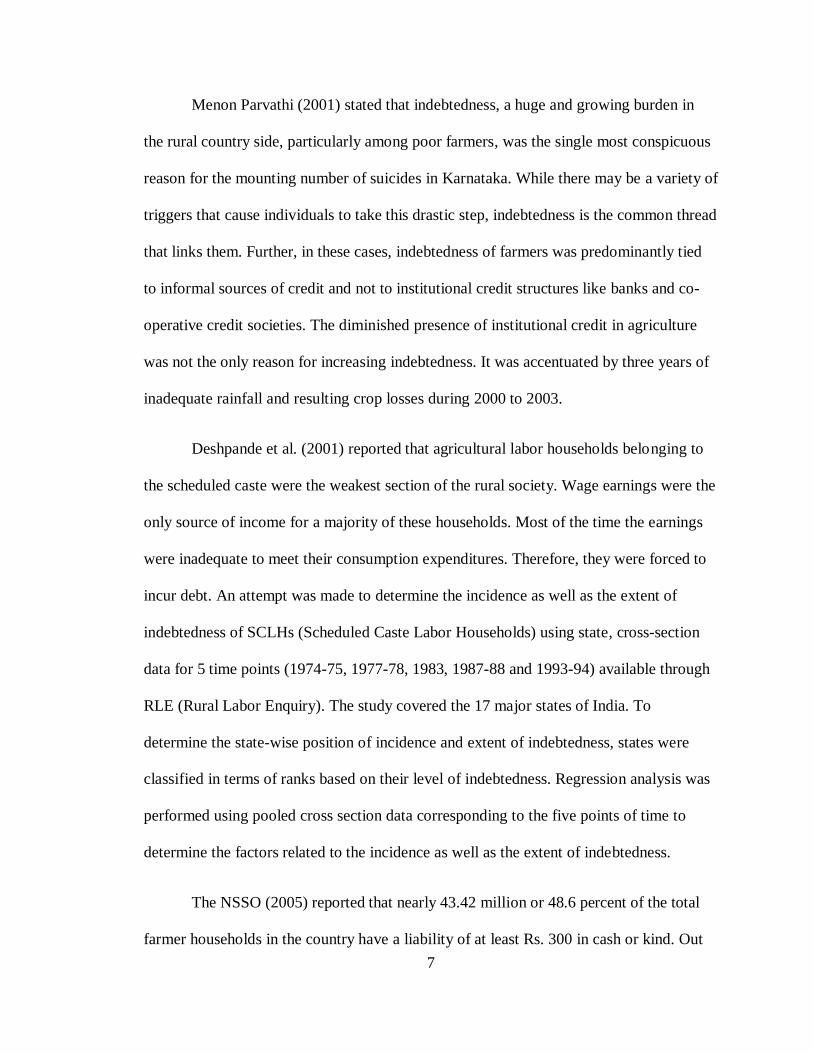
Menon Parvathi (2001) stated that indebtedness, a huge and growing burden in
the rural country side, particularly among poor farmers, was the single most conspicuous
reason for the mounting number of suicides in Karnataka. While there may be a variety of
triggers that cause individuals to take this drastic step, indebtedness is the common thread
that links them. Further, in these cases, indebtedness of farmers was predominantly tied
to informal sources of credit and not to institutional credit structures like banks and co-
operative credit societies. The diminished presence of institutional credit in agriculture
was not the only reason for increasing indebtedness. It was accentuated by three years of
inadequate rainfall and resulting crop losses during 2000 to 2003.
Deshpande et al. (2001) reported that agricultural labor households belonging to
the scheduled caste were the weakest section of the rural society. Wage earnings were the
only source of income for a majority of these households. Most of the time the earnings
were inadequate to meet their consumption expenditures. Therefore, they were forced to
incur debt. An attempt was made to determine the incidence as well as the extent of
indebtedness of SCLHs (Scheduled Caste Labor Households) using state, cross-section
data for 5 time points (1974-75, 1977-78, 1983, 1987-88 and 1993-94) available through
RLE (Rural Labor Enquiry). The study covered the 17 major states of India. To
determine the state-wise position of incidence and extent of indebtedness, states were
classified in terms of ranks based on their level of indebtedness. Regression analysis was
performed using pooled cross section data corresponding to the five points of time to
determine the factors related to the incidence as well as the extent of indebtedness.
The NSSO (2005) reported that nearly 43.42 million or 48.6 percent of the total
farmer households in the country have a liability of at least Rs. 300 in cash or kind. Out

8
of 147.90 million rural households, 60.4 percent or about 89.35 million are engaged in
farming. Estimated indebtedness was the highest in Andhra Pradesh at 82 percent
followed by Tamil Nadu at 74.5 percent and Punjab at 65.4 percent. Outstanding loan
balance per farmer was highest in Punjab, followed by Kerala, Haryana, Andhra Pradesh
and Karnataka.
Vidyasagar and Chandra (2004) reported that about 3,000 Andhra Pradesh
farmers committed suicide in five years because of the debt trap, drought and crop
failure. The government perspective on farmer suicides in India has been critically
analyzed by Vidyasagar and Chandra who argue that farmer suicides cannot be reduced
to a personal problem, but rather are related to an agrarian crisis. There was also a view
that an ex-gratia payment to the suicide victims would encourage suicides. Their study
revealed that the debt trap was the main cause of farmers taking the extreme step of
committing suicide. The debt trap tightened because of the agrarian crisis on the one hand
and inaccessibility of institutional credit on the other. No institution was lending money
to the farming community for the same purposes for which they lend money to the urban
middle class. Thus, farmers depend on non-institutional credit. In many cases, the
extreme step of suicide was taken as recourse due to the heavy pressure and humiliation
from the non-institutional sources (money lenders).
Deshpande and Nageshprabhu (2005) reported that the prevalence of indebtedness
among farmers was seen to be highest in Andhra Pradesh (82%) and lowest in
Uttaranchal (less than 10 percent). More than 50 percent of farmers availed loans for
capital or to meet current expenditures for farming purposes, 58 percent of borrowing
accrued to cultivation and other agriculture activities while the remaining percentage met

9
other consumption needs. The largest percentage of indebted farmers was in the size class
of 0.01 to 1 hectare. More than 70 percent of farmers who owned less than 2 hectares
were indebted. The average amount of loan outstanding was Rs. 12,585 (1 US dollar =
Rs. 44.895)
2.2 Extent and pattern of indebtedness of farmers to private and public financial
institution
Ramamurthy et al. (1972) found that cooperatives, commercial banks, and money
lenders were the main sources of supply of credit to sample farmers of two districts in
Tamil Nadu. The credit from the government was absent. They further showed that
cooperatives were the most important source of lending accounting for 61.73 percent,
followed by commercial banks and money lenders constituting 12.61 percent and 25.06
percent, respectively.
Manto and Torres (1975) found that even in the areas of high participation
farmers continued to seek credit from private sources at high rates of interest. This
situation signified a need to strengthen public credit sources so that farmers can acquire
credit at reasonable costs.
Sinha (1979), while studying the development and prospects of agricultural credit,
found that simultaneous functioning of multiple agencies did not succeed in providing
credit to weaker sections of the community.
Banakar and Suryaprakash (1987) studied the supply and utilization of crop
production credit in Karnataka and concluded that small and medium sized farms

10
received a lower proportion of total loans compared to their numerical strength in the
total number of borrowers, while the large farmers received a larger share.
Singh and Sharma (1990) while studying agricultural finance and management
argued that the cost of loans was one of the important basic characteristics of a good loan
and should be at a reasonable cost that involves not only interest rates but also fees for
documents and services associated with the loan.
Pouchepparadjou (1992) found that the cost of credit was more in the case of
money lenders than commercial banks because of a higher rate of interest charged by
them. Farmers were happier with commercial bank credit because the interest rate
charged was lower.
Singh and Tyagi (1995) concluded that cooperatives, by providing adequate and
timely credit could create a favorable impact on agriculture development even in
subsistence areas. This study was conducted in the Vikramjot block of Basti district of
Uttar Pradesh.
Surender S. Jodhka (1995) studied the changing structure of informal credit in
rural Haryana. His results were based on a field study of three villages selected from a
Green Revolution district in the Haryana state. He analyzed the sociology of informal
credit with a focus on understanding the changing structure of the informal credit market
and the emerging patterns of debt dependencies in light of i) the agrarian transformation
experienced with the success of the green revolution and ii) increasing availability and
growing popularity of institutional sources of credit.

11
CHAPTER 3: Methodology
This chapter outlines briefly the characteristics of the study area, the sampling
procedure, the nature and source of data, and the statistical tools and techniques
employed for analyzing the data.
3.1 Description of the study area
The present study was conducted in Hoshiarpur, Amritsar, Gurdaspur,
Kapurthala, Ludhiana, Bathinda and Ferozepur.
Figure 3.1 Location of the Study Area within India
Source: District at a glance 2005, Punjab.

12
Figure 3.2 Location of the Study Area within the Punjab State
Source: District at a glance 2005, Punjab.
3.1.1 Hoshiarpur district
The Hoshiarpur district falls in the eastern part of the Punjab State and covers an
area of 3,365 sq. km. The district is drained by the river Beas in the north and northwest
and Satluj in the south. The main townships are Hoshiarpur-I and Hoshiarpur-II.
Administratively the district has four tahsils, five sub-tahsils, and ten blocks. The tahsils
are Hoshiarpur, Dasuya, Garh Shankar, and Mukerian. The blocks are Hoshiarpur-I,

13
Hoshiarpur-II, Bhunga, Tanda, Dasuya, Garh Shankar, Mahipur, Mukerian, Talwara, and
Hajipur. The district is the second lowest densely populated district of the state. The total
population of the district as per the 2001 census is 1,480,736. The population density is
440 persons per square kilometer. The decennial growth rate of population in the district
for the decade 1991-2001 was 14.02 percent. A majority of population in the district live
in rural areas (i.e., 80.28% of population (1,188,662) live in rural areas; 19.72%
(292,074) live in urban areas). The land utilization pattern and details of demographic
features of the study area are presented in Table 3.1 and Table 3.2 respectively.
The climate of Hoshiarpur district is classified as tropical steppe, hot, and semi-
arid, and is mainly dry with very hot summers and cold winters except during the
monsoon season when the moist air of oceanic origins penetrates the district. There are
four seasons a year. The hot weather season starts from mid-March to the last week of
June followed by the southwest monsoon which lasts up to September. The transition
period from September to November forms the post monsoon season. The winter season
starts late in November and remains to the first week of March.
The normal annual rainfall of the district is 938 mm which is unevenly distributed
over the area in 38 days. The southwest monsoon contributes about 77% of annual
rainfall. July and August are the wettest months. The remaining 23% of rainfall is
received during the non-monsoon period in the wake of western disturbances and
thunderstorms. Generally, rainfall in the district increases from southwest to northeast.
The information on cropping patterns of the district is presented in the Table 3.3.
The district forms a part of Indo-Gangetic plain and Sutlej sub-basin of the main
Indus basin. The area comprises three distinct geomorphologic units, a hilly area in the

14
northeast, the piedmont zone belt, and the alluvial plains in the southwestern part of the
district. The soils are yellowish brown to dark brown in color. These range from
calcareous sand to fine sandy loam to silt. Sand is mostly cultivated and is well drained
with an estimated infiltration rate of 8-10 cm/hour.
3.1.2 Amritsar district
The Amritsar district is located in the northern part of the Punjab state. The total
area of the district is 5056 sq. km. Amritsar I, Amritsar II, Baba Bakala and Ajnala are
four teshils of the district. Majitha, Attari, Tarsikka, Lopoke, and Ramdas are sub tehsils
in the district. There are eight development blocks namely Tarsikka, Rayya, Ajnala,
Chogawaan, Majitha, Verka, Jandiala Guru, and Harsha China. The population of the
district was 2,157,020 as per the 2001 census which constitutes 8.85% of the total
population of the state. The total population of the Amritsar district in 1991 was
1,745,252 and indicated a 23.59% decennial growth from1991 to 2001. The population
density of the district is 804 persons per square kilometer versus the state average of 484
persons per square kilometer. The Amritsar district falls between river Ravi and Beas.
The land utilization pattern of the study area is presented in Table 3.1. Table 3.2 presents
details of demographic features.
The climate of the district is classified as tropical steppe, semi-arid, and hot; and
is mainly dry with a very hot summer and cold winter except during the southwest
monsoon season. There are four seasons in a year namely the cold season from
November to March, the hot season from April to June, the southwest monsoon season
from the last week of June to the middle of September, and the post monsoon season
from September to the beginning of November. During the cold season, a series of

15
western disturbances affect the climate of the district. The normal annual rainfall of the
district is 680 mm unevenly distributed over 31 days. The southwest monsoon contributes
75% of yearly rainfall and sets in the last week of June and withdraws in the middle of
September. The remaining 25% of annual rainfall occurs in the non-monsoon months.
The rainfall increases from the southwest to the northeast in the district. The information
on cropping patterns for the district is presented in Table 3.3.
The Amritsar district falls in between Ravi river and Beas river. The Ravi river
flows in the northwest of the district and forms the international border with Pakistan.
The Beas river flows in the eastern part of the district. The soils in the western part of the
district are coarse loamy, calcareous soils, whereas in the central part of the district, the
soils are fine loamy, calcareous, and are well drained. The soils are Ustochrepts to
Haplustaff types.
3.1.3 Gurdaspur district
The Gurdaspur district is located in the northern most part of the Punjab state. It
shares the boundary with Jammu and Kashmir and Himachal Pradesh. The district is
bounded by the Ravi and Beas river. It has a unique characteristic of sharing the
international boundary with Pakistan. Hoshiarpur, Kapurthala, and Amritsar are situated
on the eastern, southern, and western side of the district, respectively. It covers an area of
3,513 square kilometer and forms a part of the upper Bari Doab area. Physiographically,
the area is divided into three units (i) the Siwalik Hills lying in northeast of the district,
(ii) the Kandi Zone lying immediately southwest of the foothill zone of Siwalik hills, (iii)
and the Alluvial plains lying southwest of Kandi. The district is divided into five tehsils
and 16 development blocks for the purposes of administrative control. The land

16
utilization patterns and demographic features of the study area are presented in Table 3.1
and Table 3.2, respectively.
The normal annual rainfall of the area is 1113 mm which is unevenly distributed
over the district. The southwestern monsoon (July to September) contributes about 80%
of the rainfall and the rest occurs during the non-monsoon period. The rainfall in the
district increases from the southwest to the northeast. The highest annual rainfall of 1443
mm, 30% more than the normal, was recorded in 1988 and the lowest of 615 mm, 44%
less than the normal, was experienced in 1989. The climate of the district is tropical with
four well defined seasons. The maximum temperature is 41 C and minimum is 6 C. The
information on cropping patterns for the district is presented in Table 3.3.
The district can be divided into three geomorphologic types-a Hilly area, a
Piedmont zone, and an alluvial plain. The hilly area is predominately on the northeast
part of the district and called Siwalik which are mainly clays and clay with boulders. The
Dherkalan block is predominantly covered by hilly terrain. The Piedmont comprises
pebbles, and cobbles drain from the Siwalik along with sand of medium to coarse grained
gravel. The alluvial plain is sand intercalated with clays deposited by the rivers Ravi and
Beas.
3.1.4 Kapurthala district
The Kapurthala District is situated in the Bist Doab and comprises two
noncontiguous parts separated by some 32 kilometers. Kapurthala, Sultanpur Lodhi and
Bholath Tehsils form one part and Phagwara Tehsil, the second separated portion. The
geographical area of the district is 1,633 square kilometer. The Kapurthala District is
bounded partly in the North and wholly in the West by the Beas River, named as the
Hydaspes River. The Kapurthala district is surrounded by Amritsar in the West,

17
Hoshiarpur in the North, Jalandhar in the east, and Firozepur in the South. The Phagwara
block is surrounded on three sides, the northwest, west, and southwest by the Jalandhar
District, on the northeast and east by Hoshiarpur District, and by Nawan Shehar in the
south. The Kapurthala district ranks 13th in the Punjab with a population of 754,521
which is 3% of the total population of the Punjab state. The population density is 461 per
square kilometer. The literacy rate is 73%. Sixty seven percent of the population lives in
rural areas while the remaining 33% lives in urban areas. The land utilization pattern and
details of demographic features of the study area are presented in Table 3.1 and Table
3.2, respectively.
The climate of the district is characterized by general dryness except for a short
period during the southwest monsoon season. There are four seasons a year namely the
cold season from November to March, the hot season from April to June, the monsoon
season from the last week of June to the middle of September, followed by post monsoon
season through the beginning of November. During the cold season, a series of western
disturbances affect the climate. During the summer months (i.e., from April to June) the
weather is very hot, dry, and uncomfortable. The weather becomes humid and cloudy
from July to September with the penetration of moist air of oceanic origin in the
atmosphere.
The normal annual rainfall of the district is 779 mm, which is distributed over 33
days a year. The southwest monsoon contributes 75% of the rainfall and sets in the last
week of June and withdraws in the middle of September. July and August are the rainiest
months. The information on the cropping patterns of the district are presented in the
Table 3.3.

18
The Kapurthala district is occupied by Indo-Gangetic alluvim soil. The major
portion of this region lies in the river tract falling between the Beas and Black Bein and is
called „BET‟. To the south of the Black Bein lies the tract known as „Dona‟. The word
„Dona‟ means that the soil is formed of two constituents, sand and clay, with sand
predominating. The numerous streams coming down from Hoshiarpur district keep the
soil moist all year. Some of the streams are silt laden and at first deposit fertile soil
though later deposits are more sandy. Due to the existence of drainage channels, patches
and strata‟s of hard clay are also found. The major soil types in the district are the arid
brown soils and tropical arid brown soils. The arid brown soils are found mostly in the
southern parts of the district and the tropical arid brown soils are found in the northern
part and Phagwara block of the district. The arid brown soils are calcareous in nature and
tropical arid brown soil is deficient in nitrogen, potassium, and phosphorus.
3.1.5 Ludhiana district
The Ludhiana district falls in the central part of Punjab. The Satluj forms the
border of the district in the north with the Jalandhar and Hoshiarpur districts. The Ropar
and Fatehgarhsahib districts mark the eastern and southeastern boundaries. The western
border adjoins the Moga and Ferozpur districts. The geographical area of the district is
3790 square kilometers. Administratively, Ludhiana falls under the Patiala division. The
district has four sub-divisions, Ludhiana, Khanna, Samrala, and Jagraon, and eleven
development blocks: Ludhiana, Mangat, Doraha, Khanna, Dehlon, Pokhwal, Samrala,
Machiwara, Jagraon, Sidhwanbet, and Sudhar. The land utilization patterns and details of
demographic features are presented in Table 3.1 and Table 3.2 respectively.
The climate of the Ludhiana district can be classified as tropical steppe, hot, and
semi-arid; and is mainly dry with very hot summers and cold winters except during the

19
monsoon season when the moist air of oceanic origin penetrates into the district. There
are four seasons. The hot weather season starts from mid-March to the last week of June,
followed by the southwest monsoon which lasts up to September. The transition period
from September to November forms the post-monsoon season. The winter season starts
late in November and remains up to the first week of March.
The normal annual rainfall of the district is 680 mm which is unevenly distributed
over the area in 34 days. The southwest monsoon sets in from the last week of June and
withdraws at the end of September and contributes about 78% of annual rainfall. July and
August are the wettest months. Generally, rainfall in the district increases from the
southwest to the northeast. The information on cropping patterns for the districts is
presented in the Table 3.3.
The district is occupied by Indo-Gangatic alluvium soils. There are no surface
features except that the area is a plain with its major drains being the Satluj and its
tributaries. The soil is the end product of the parent material resulting from the influence
of climate, topography, and the natural vegetation over a long period of time. In the
district, soil characteristics are influenced to a very limited extent by the topography,
vegetation, and parent rock. The variations in the soil profile are much more pronounced
because of the regional climatic differences. The soil of this zone has developed under
semi-arid conditions. The soil is sandy loam to clay with a normal pH from 7.8 to 8.5.
3.1.6 Bathinda
The Bathinda district is situated in the southern part of Punjab. It covers an area of
3367 square kilometer. The district is surrounded by the Sirsa and Fatehabad districts of
the Haryana State in the south, the Sangrur and Mansa districts in the east, the Moga in
the northeast, and the Faridkot and Muktsar districts in the northwest. The Bathinda

20
district has three sub-divisions: Bathinda, Rampura phul, and Talwandi Sabo. It has seven
blocks: Bathinda, Nathana, Rampura, Phool, Talwandi Sabo, Sangat, and Maur. The
district has a good network of canals for irrigation and domestic water use. The land
utilization patterns and demographic features of the study area are presented in Table 3.1
and Table 3.2, respectively.
The climate of the Bathinda district can be classified as tropical steppee, semi-arid
and hot; and is mainly dry except in rainy months and characterized by an intensely hot
summer and cold winter. During the three months of monsoon season from July to
September, the moist air of oceanic origin penetrates into the district and causes high
humidity, cloudiness, and a good monsoon rainfall. The period from October to
November constitutes the post monsoon season. The cold weather season prevails from
December to February followed by the hot weather season that ends the last week of
June.
The normal annual rainfall of the Bhatinda District is 408 mm in 20 days which is
unevenly distributed over the district. The southwest monsoon sets in the last week of
June and withdraws towards the end of September, and contributes 82% of annual
rainfall. July and August are the rainiest months. The rainfall in the district increases
from southwest to northeast. The information on cropping patterns is presented in the
Table 3.3.
The district area is occupied by Indo-Gangetic alluvim soils. The maximum
elevation in the area is 220.6 m. and the minimum elevation is 197.5 m. The master slope
of the area is towards the southwest. The southern part contains isolated sand dunes of
various dimensions. The district has two types of soils, the arid brown soils and siezoram

21
soils. The arid brown soils are calcareous in nature. These soils are imperfectly to
moderately drained. Salinity and alkalinity are the principal problems of this soil. In
siezoram soils, the accumulation of calcium carbonate is in the amorphous or
concretionary form. The presence of a high amount of calcium carbonate and poor
fertility are the main problems of this soil. The arid brown soils are found mostly in the
eastern parts of the district and the siezoram soils are found in the western parts of the
district.
3.1.7 Ferozepur
The Ferozpur district is the southwestern most district of Punjab with a total
geographical area of 5850 square kilometer. Administratively, the district is under the
control of the Ferozpur division and is divided into five sub-divisions, Ferozpur, Fazilka,
Abohar, Zira, and Jalalabad; and four sub tehsils; Arniwala Sheikh Subhan, Mamdot,
Talwandi Bhai, and Makhu. The Ferozpur district forms a part of Sutlej sub-basin of
main Indus basin and is interrupted by clusters of sand dunes. The district contains almost
a flat terrain with a gentle slope towards the southwest. Physiographically, it is
characterized by four distinct features, the upland plain, sand dune tracts, younger flood
plain, and active flood plain. The river Sutlej is of a perrineal nature that mainly drains
the area. The river Sutlej shows both the influent and effluent nature in the area. The area
is traversed by a dense network of canals. In terms of irrigation practices, the contribution
of tube wells is large compared to the canal system. The land utilization patterns and
demographic features of the study area are presented in Table 3.1 and Table 3.2,
respectively.
22
The climate of the district can be classified as tropical desert, arid, and hot. The
area receives about 389 mm of annual rainfall that is unevenly distributed over the area in
23 days, out of which about 79% occurs during the southwest monsoon season. The
rainfall in the district decreases from northeast to southwest. Information on cropping
patterns is presented in the Table 3.3.
The district forms a part of Indo-gangetic plain and the Sutlej sub basin of the
main Indus basin. The area as a whole is almost flat with a gentle slope towards the
southwest. The physiographic of the district is broadly classified from north to south into
four distinct features, Upland plain, Sand dune tract, younger flood pain, and active flood
plain of Sutlej. The soil of the district is of two types (i.e., sierozem (in northern parts)
and desert soils (in southern parts)).

23
Table 3.1: Land Utilization Pattern in Selected Districts
Districts
Item Hoshiarpur Amritsar Gurdaspur Kapurthala Ludhiana Bathinda Ferozepur
Total Geographical area (sq. km.) 3364 5094 3560 1633 3680 3382 5850
Area under forest (sq. km.) 1000 100 213 20 100 8 -0.12
Cultivable area (sq. km.) 3410 4260 2850 1350 6080 297 0.0247
Other uncultivated land (ha) 1000 1000 2000 1000 0 0 2000
Fallow land (ha) below 500 below 500 0 1000 5000 0 below 500
Net sown area (sq. km.) 2180 2220 2850 1350 3250 297 0.0133
Net irrigated area (sq. km.) 1570 2220 2360 1350 3060 2910 4735
Source: Statistical abstract of Punjab, 2005

24
Table 3.2: Socio-Economic Features of the Study Area
Districts
Variables Hoshiarpur Amritsar Gurdaspur Kapurthala Ludhiana Bathinda Ferozepur
Number of inhabited village (No.) 1386 1185 1532 618 897 280 968
Total Population (No.) 1480736 3096077 2104011 754521 3032831 1183295 1746107
a. Rural 1188662 1872802 1568788 507994 1339178 831541 1295382
b. Urban 292074 122327 535223 246527 1693653 351754 450725
c. Male 765132 1650589 1113077 399623 1662716 632809 926224
d. Female 715604 1445488 990934 354898 1370115 550486 819883
Population density (persons/sq.km.) 440 608 590 462 805 350 329
Literacy rate (%) 81.0 67.3 73.8 73.9 76.5 61.2 60.7
a. Male 86.5 72.6 79.8 79.0 80.3 67.8 68.7
b. Female 75.3 61.3 67.1 68.3 71.9 53.7 51.7
Normal rainfall (mm) 523.7 303.1 761.1 230.9 270 209.5 32.1
Agricultural holding (ha)
a. Marginal holdings 23887 19763 27581 5980 9924 8779 11238
b. Small holdings 18937 25739 22467 7498 12696 7565 12798
c. Medium holdings 23627 46303 32901 13274 17756 14147 29655
d. Large holdings 15810 35408 22246 9368 20515 19603 36824
Source: Statistical abstract of Punjab, 2001

25
Table 3.3: Area under Major Crops in the Study Area (thousand hectares)
Districts
Variables Hoshiarpur Amritsar Gurdaspur Kapurthala Ludhiana Bathinda Ferozepur
Cereals
Paddy 58 334 202 105 247 102 238
Maize 64 4 13 3 2 1 0
Wheat 145 372 227 115 258 241 386
Barley 0 0 0 0 0 1 1.4
Pulses 0.4 1.1 0.7 0.2 1.7 1.1 1.4
Oilseeds 1.9 1.6 1.2 0.5 0.3 1.1 1.5
Commercial Crops
Cotton 0 0.1 0 0 0.2 129 123
Sugarcane 18 7 20 5 3 0 2
Source: Statistical abstract of Punjab, 2005
26
Table 3.1 shows the land utilization patterns in selected districts of Punjab for
2005. The data were collected for each district by the Punjab state department. The total
geographical area was the highest in Ferozepur followed by Amritsar, Ludhiana,
Gurdaspur, Bathinda, Hoshiarpur, and Kapurthala. The net-sown area was highest in
Ludhiana, followed by Gurdaspur, Amritsar, Hoshiarpur, Kapurthala, Bathinda and
Ferozepur. This indicates that Ferozepur, having the highest geographical area, has the
lowest cultivable area and net-sown area.
Table 3.2 shows the socio-economic features in the selected districts of the
Punjab. The data were collected for each district in 2001 by the Punjab state government.
Ludhiana had the highest population density followed by Amritsar, Gurdaspur,
Kapurthala, Hoshiarpur, Bathinda, and Ferozepur. The literacy percentage was the
highest in Hoshiarpur, followed by Ludhiana, Kapurthala, Gurdaspur, Amritsar,
Bathinda, and Ferozepur. We can also observe from the table that a majority of the
farmers fall into small and medium land holdings.
Table 3.3 shows the area under major crops in selected districts of Punjab.
Farmers mainly grow wheat, paddy, and maize and do not concentrate on pulses, oil
seeds, and commercial crops. This is one of the reasons why farmers may not be able to
repay loans. They follow traditional cropping patterns. Farmers may need to adopt newer
cropping systems that involve cash crops.
3.2 Sampling procedure
A random sampling procedure was adopted for the selection of the district, taluks,
villages, and cultivators to collect the required information for this research (Dr. Rajinder
Sidhu).

27
3.3 Data
For evaluating the specific objectives of the study, primary data were obtained
from families in suicide prone areas through personal interviews with the help of a
structured survey. The data collected pertained to agriculture for the year 2005. The data
collected from respondents included general information about the farmer, their resource
position, land holdings, cropping patterns, debt condition, sources of income, asset
position, sources of credit, and any other information the family wished to share. The
researchers were able to interact with the next of kin in the family and other members of
the family in addition to the farmer to get the required information. The method of
personal interview was adopted to ensure that the data obtained from the respondents
were relevant, comprehensive, consistent, and reasonably correct.
3.4 Analytical techniques employed
For the purpose of achieving the specific objectives of the study, the data were
subjected to the following analysis.
3.4.1 Tabular analysis – Ratio’s, percentages
Tabular analyses involves the computation of means, percentages, etc, that were
used to present the data regarding demographic features, socio-economic profile,
cropping systems, costs, and returns of the farmers. Similarly, data pertaining to different
sources of income were also computed.
3.4.2 T-test
A t-test is any hypothesis test in which the test statistic follows a simple t-
distribution if the null hypothesis is true. It is most commonly applied when the test

28
statistics would follow a normal distribution if the value of a scaling term in the test
statistics were known. When the scaling term is unknown and is replaced by an estimate
based on data, the test statistics follows a simple t-distribution.
3.4.3 Farm Business Analysis Tool
Ratios are important measurements to analyze the performance of any business
organization. Relevant financial ratios determined for the farm enterprises were the debt
equity ratio, debt asset ratio, net worth, and net capital ratio.
3.4.4 Debt-Equity Ratio (Leverage)
This ratio is also known as the leverage ratio. It indicates what proportion of
equity and debt the company is using to finance the asset base. It compares the owner‟s
stake in the business with outside liabilities. A lower value of the ratio indicates that
leverage is small and the major capital being equity.
Debt-Equity ratio = WorthNet
sLiabilitieLongterm
In the above ratio, debt represents only long term liabilities and not current
liabilities, while equity refers to net worth after deducting intangible assets. Net worth
includes statutory reserves and share capital.
3.4.5 Debt Asset Ratio (DAR)
The Debt Asset Ratio (DAR), is a ratio of amount of debt to amount of assets per
farm. The higher the value of DAR the higher the risk.
Debt asset ratio = AssetsTotal
sLiabilitieTotal

29
3.4.6 Net Worth
Net worth indicates what the business owes to the owners of business. It measures
the excess of assets compared to liabilities and indicates the soundness of the business.
Net worth = sLiabilitieTotalAssetsTotal
3.4.7 Net Capital Ratio
This ratio indicates the degree of liquidity in a business for the long term. It
measures the availability of assets to pay long term liabilities.
Net Capital Ratio = sLiabilitieTotal
AssetsTotal
The higher the net capital ratio, the greater the margin of safety against a decline
in the prices of major assets.
3.4.8 Logistic Regression Model
Based on the survey, the data were categorized into farmers‟ who are indebted
and farmers‟ who are non-indebted. Debt use (indebted or non-indebted) was
hypothesized to depend on the farmers‟ age, education, family size, landholding,
occupation, and net income. The influence of various socio-economic factors on the
probability of incidence is often investigated using logit analysis (Mishra, 2006). In this
thesis, five types of models were estimated using Stata: logit, tobit, McDonald and
Moffitt decomposition, probit, and the heckman two-step method.
The logit model was used to analyze the probability of a farmer being indebted or
non-indebted. The tobit model was used for the data that were censored. Decomposition

30
was used to analyze the conditional mean functions in the tobit model. The probit model
was used to construct the selection bias control factor. The heckman two step method was
used to remove the bias in the results. All these models were used for different purposes
in this study.
The logit model assumes that the probability of an individual, i, being indebted
has the form (Mishra, 2006):
Pi = P (Yi=1/Xi) = eX
iβ / (1+e
Xiβ)
where Xi is the set of explanatory variables that include individual characteristics and β is
the set of unknown parameters. Similarly, the probability of an individual being non-
indebted is:
1-Pi = P (Yi=0/Xi) = 1 / (1+eX
iβ)
Taking the ratio of the two expressions we get
P (Yi=1) / P (Yi=0) = eXiβ
Taking the natural log of both sides we get
ln [Pi / (1-Pi)] = Xβ = β0 + β1X1 + β2X2 + … + βnXn
These parameters can be estimated using maximum likelihood estimation techniques. The
logit model guarantees probabilities in the range of (0, 1).
The specific LOGIT model to predict the odds of a farmer being indebted is
specified as follows:
ln [Pi/(1-Pi)]=β0+β1X1+β2X2+β3X3+β4X4+β5X5+β6X6

31
where Pi= probability that the ith
farmer will be indebted,
1-Pi= Probability that the ith
farmer will not be indebted,
Age (X1) = The respondents were asked their actual age in years,
Education (X2) = The respondents were asked for their education level,
Family size (X3) = The respondents were asked for the number of people in the family,
Landholding (X4) = The respondents were asked for their total farm size (land holding),
Occupation (X5) = Occupation (0 = Agriculture; 1 = Agriculture + Business), and
Net-income (X6) = Net income calculated in rupees
3.4.9 Tobit Model
Tobit analysis is used for data that are censored, meaning that the dependent
variables have several observations clustered at a lower or upper limiting value. Tobit
analysis includes all observations, including those at the limit, to estimate the regression
parameters. Tobit analysis corrects for omitted variable bias and accounts for the fact that
the expected values of the errors are changing.
3.4.10 Tobit model for censored observations
Censoring occurs when data on the dependent variable is lost or limited but not
data on the regressors. Censoring is a defect in the sample – if there were no censoring,
the data would be a representative sample from the population of interest.

32
When the distribution is censored on the left, observations with values at or below
0 are set to
Y =
0*0
0**
yif
yify
The Tobit model is:
If Xβ + e > 0, then y = Xβ + e
If Xβ + e ≤ 0, then y = 0,
where X represents the independent variables, β is the Tobit coefficient corresponding to
the independent variables, and e is an error term with a normal distribution (Roncek,
1992). A combination of these two equations results in the total derivative for Tobit
analysis.
3.4.11 Expected Values for Tobit Model (Decomposition)
The expected value of y when y is greater than 0:
E[y|y > 0] = Xiβ + σλ(α)
where λ(α) =
i
i
X
X
is the inverse mills ratio. (.) is the standard normal probability
distribution function and (.) is the standard normal cumulative distribution function.
The expected value of y when y is equal to 0:

33
E[y] = Ф
iX [Xiβ + σλ(α)]
where λ(α) =
i
i
X
X
is the inverse mills ratio. (.) is the standard normal probability
distribution function and (.) is the standard normal cumulative distribution function.
This is the probability of being uncensored multiplied by the expected value of y given y
is uncensored. This is known as the McDonald and Moffitt‟s decomposition.
3.4.12 Estimation with Heckman’s Two-Step Procedure
The Heckman approach corrects for selection bias in the data. Selection bias may
arise when a sample does not randomly represent the underlying population. The inverse
mills ratio (Heckman) controls for selection bias and including it allows for unbiased
coefficient estimates.
There are basically two versions of selection bias. In the standard case of selection
bias, information on the dependent variable for part of the respondents is missing.
Secondly, information on the dependent variable is available for all respondents, but the
distribution of respondents over categories of the independent variable we are interested
has taken place in a selective way. This kind of bias is also called as heterogeneity bias.
Heckman proposed a two-step procedure that involves the estimation of a
standard probit and a linear regression model. In the first step, the standard probit model
is estimated and a selection bias control factor called Lambda is constructed. This factor
reflects the effects of all unmeasured characteristics in the model.

34
Prob(y=1|X1,X2,X3,X4,X5,X6) = Ф (β1X1,β2X2,β3X3,β4X4,β5X5,β6X6)
where y is 1 if indebted and 0 otherwise, X1, X2, X3, X4, X5, X6 are vectors of explanatory
variables. βs are unknown parameters and Ф is cumulative distribution function of the
standard normal distribution.
Estimation of the model yields results that can be used to predict the probability
of each individual being in debt.
In the second step, a regression model is estimated along with the selection bias
control factor lambda (inverse mills ratio) as an additional independent variable. Because
this factor reflects the effects of the unmeasured characteristics related to the
indebtedness decision, the coefficient of this factor in the analysis catches the part of the
effect from these characteristics that are related to non-indebtedness. Because we have a
control factor in the analysis for the effect of the indebtedness, the other predicators in the
equation are free from this effect and the regression analysis produces unbiased
coefficients for them.
The loan equation is specified as:
L* = β1age + β2education + β3family size + β4landholding + β5occupation +β6net-income
+ u
where L* denoted the total amount borrowed in rupees. The conditional expectation of
loan given the farmer takes the loan is then
E [L|X1,X2,X3,X4,X5,X6, y=1] = β1X1+β2X2+β3X3+β4X4+β5X5+β6X6+ e
Under the assumption that the error terms are jointly normal, we have
E [L|X1,X2,X3,X4,X5,X6, y=1] =
β1X1+β2X2+β3X3+β4X4+β5X5+β6X6+ ρσuλ(β1X1+β2X2+β3X3+β4X4+β5X5+β6X6)

35
where ρ is the correlation between unobserved determinants indebtedness. The term, σu is
the standard deviation of u, and λ is the inverse mills ratio evaluated at
β1X1+β2X2+β3X3+β4X4+β5X5+β6X6
Applying the theoretical model in practice is not straight forward. An important
condition for its use is that the main equation contains at least one variable not related to
the dependent variable in the lambda equation. If such a variable is not present (and
sometimes even if such a variable is present), there may arise severe problems of
multicollinearity and the addition of the correction factor (lambda) may lead to estimation
difficulties and unreliable coefficients.

36
CHAPTER 4: Results
4.1 Socio-Economic Profile of the Sample Respondents
To understand the nature and cause of indebtedness, the socio-economic profile of
the sample respondents was studied.
4.1.1 Age
Age was categorized into three groups, less than 35 years, 36-50 years, and more
than 50 years (Table 4.1; Figure 4.1). The average age of indebted farmers was 48.72.
The middle age group is more likely to be in debt than younger or older farmers. This is
the age when a large number of decisions are made for the households. A majority of the
respondents belonged to 36-50 years age group (45 percent). The remaining 37.5 percent
belonged to the older age group and remainder (17.5 percent) in the younger age group.
The average age of sample respondents without debt was 47.69. The mean t-test for age
variable is statistically significant at 1 percent level indicating a statistical difference
between the age of indebted and non-indebted individuals.
4.1.2 Education Level
The education level of farmers was categorized into four groups, illiterate,
primary, secondary, and college education (Table 4.1; Figure 4.2). A majority of farmers
who were indebted were educated up to primary level (45.45%). About 26 % were
illiterate, about 20% were educated up to secondary level, and 8% were educated up to
college level. Among non-indebted farmers, 40% had secondary education followed by
primary (30%), illiterate (25%), and college education (5%). The mean t-test for

37
education variable is statistically significant at 5 percent levels indicating a statistical
difference between education of indebted and non-indebted farmers.
Table 4.1: Social Charteristics of the Sample Respondents
Particulars Indebted Farmers
Non-indebted Farmers
Frequency % Frequency %
Age
Young (<35) 27 12.27 14 17.5
Middle (36-
50)
108 49.09 36 45
Old (>50) 85 38.64 30 37.5
Average 48.72
47.69
Education
Illiterate 58 26.36 20 25
Primary 100 45.45 24 30
Secondary 44 20.00 32 40
College 18 8.18 4 5
Average 6.67
5.85
Family Size
Male 447 39.56 155 35.71
Female 384 33.98 150 34.56
Children 299 26.46 129 29.72
Total 1130 100 434 100
Average 5.14
5.43

38
Figure 4.1: Social Characteristics of Indebted Farmers- Age
Figure 4.2: Social Characteristics of Indebted Farmers- Education

39
4.1.3 Family size
Family size included the number of male, female and children in the family. The
average family size was slightly smaller with an average number of 5.14 for the indebted
farmers when compared to non-indebted farmers (5.43). Within the family there was not
much difference in the distribution of the male, female, and children of both indebted and
non-indebted farmers. The mean t-test for family size variable is statistically significant 5
percent level indicating a statistical difference in family size among the with and without
debt.
4.1.4 Land Holding
Land holding was categorized into four groups, less than 1 hectare, 1 to 2
hectares, 2 to 4 hectares, and more than 4 hectares (Table 4.2). An analysis of the
distribution of various land holding categories revealed that among the indebted farmers a
majority of the farmers had between 2 and 4 hectares (35.45 percent) or more than 4
hectares (30.91 percent). Among the non-indebted farmers, a majority of the farmers had
between 2 and 4 hectares (28.75 percent) and between 1 and 2 hectares (26.25 percent).
The mean t-test for landholding variable is statistically significant at 1 percent level
indicating a statistical difference in landholding with and without debt.
4.1.5 Occupational pattern
Occupational patterns of sample respondents (Table 4.2) revealed that a majority
of farmers were dependent on agriculture. Among the indebted farmers, 93% were
dependent upon agriculture and the remaining had a supplementary business (7%).
Among the non-indebted farmers, 90% depended upon agriculture. The percentage of

40
farmers with a supplementary business was slightly higher than that of indebted farmers
(10%).
A greater dependency of farmers on farming with negligible supplementary
enterprises indicates a vulnerability to natural and financial risks. The mean t-test for
occupational pattern variable is not statistically significant at 10 percent level.
Table 4.2: Agro-Economic Profile of Respondents
Particulars Indebted
Farmers
Non-indebted
Farmers
Frequency % Frequency %
Land holdings
Marginal (<1ha) 25 11.36 16 20
Small (1-2ha) 49 22.27 21 26.25
Medium (2-4ha) 78 35.45 23 28.75
Large (>4ha) 68 30.91 20 25
Total 220 100.00 80 100
Occupational Pattern
Agriculture 205 93.18 72 90
Agriculture + Business 15 6.82 8 10
Total 220 100 80 100
Total Land Holding (ha) 748.81
235.09
Average Land Holding (ha) 3.40
2.94

41
4.1.6 Distribution of indebtedness by retrospectively reconstructed reasons
Various reasons have been suggested as causes for farmers‟ indebtedness. In this
study, the method of retrospectively reconstructed reasons was adopted to determine the
probable causes for farmers‟ indebtedness (Table 4.3; Figure 4.3).
The most predominant reason as revealed by respondents was for agricultural debt
(Table 4.3). About 41 percent of the respondents ascribed agriculture debt to be the major
factor. This was followed by others like medical treatment (13.28%), excessive social
expenditure (12.11%), and education (10.35%). Other causes reported were agriculture
activity (5.86%), purchase of gold (5.47%), and religious functions (5.47%).
Table 4.3: Distribution of Indebtedness Cases by Retrospectively Reconstructed
Reasons
Reasons for Indebtedness Number Percentage
Excessive Social Expenditure 62 12.11
Purchase of gold 28 5.47
Religious functions 28 5.47
Education 53 10.35
Medical Treatment 68 13.28
Education (abroad) 2 0.39
Purchase of land 4 0.78
Agriculture Debt 212 41.41
Agriculture activity 30 5.86
Any other 25 4.88

42
Figure 4.3: Distribution of Indebted Cases by Retrospectively Reconstructed
Reasons

43
4.2 Farm Business Performance
4.2.1 Cropping patterns of Indebted and Non-indebted farmers
An examination of cropping patterns on the farms of sample respondents is
presented in table 4.4. There was not much difference in the cropping pattern of the two
types of farms.
In the kharif season, farmers that were indebt grew kharif paddy (23.68%), cotton
American (17.53%), kharif fodder (6.25%), and maize (1.93%). Other crops grown were
vegetables, sugarcane, and kharif oilseeds. Similar patterns were noticed on the farms of
non-indebted farmers. They grew Kharif paddy (25.20%), kharif fodder (11.35), maize
(4.73%), and cotton American (4.41%).
In the rabi season, farms with and without debt had similar cropping patterns.
Wheat was the dominant rabi crop. Farms with debt grew wheat (44.24%), rabi fodder
(4.60%), and rabi oilseeds (.04%). The crops of farmers without debt were wheat
(44.27%), rabi fodder (7.65%), and rabi pulses (0.04%).

44
Table 4.4: Cropping Pattern of the Farms of Indebted and Non-indebted Farmers
Season Crop Indebted Farmers Non-indebted Farmers
Area (ha) Percent Area (ha) Percent
Kharif Paddy 353.94 23.68 138.59 25.20
Cotton American 262.02 17.53 24.28 4.41
Cotton Desi 0 0.00 0.28 0.05
Maize 28.8 1.93 26.04 4.73
Sugarcane 5.6 0.37 10.2 1.85
Kharif Pulses 0 0.00 0.2 0.04
Kharif Oilseeds 0.6 0.04 0 0.00
Kharif Fodder 93.49 6.25 62.43 11.35
Vegetable 17.6 1.18 1.6 0.29
Fruits 0 0.00 0 0.00
Others 1.6 0.11 0 0.00
Rabi Wheat 661.28 44.24 243.45 44.27
Barley 0 0.00 0 0.00
Rabi Pulses 0 0.00 0.2 0.04
Rabi Oilseeds 0.6 0.04 0.6 0.11
Rabi Fodder 68.81 4.60 42.08 7.65
Others 0.4 0.03 0 0.00
Total 1494.74 100.00 549.95 100.00

45
4.2.2 Cost-return Profile of Major Crops Grown by the Respondents (Rs. /hectares)
To calculate the cost-return profile of major crops the following equations were
used.
Cost A = seed cost + fertilizer cost + pesticide cost + hired labor + hired
machinery + rent paid for leased land.
Cost B = Cost A + interest on fixed capital excluding land.
Cost C = Cost B + input value of family labor.
Farm Business Income = Gross returns – Cost A
Family Labor Income = Gross returns – Cost B
Net Income = Gross returns – Cost C
The relative profitability of major crops was determined by farm business
analysis. Farm business income is a difference between gross returns and cost A whereas
net income is the difference between gross returns and cost C.
Among the indebted farms, out of the three crops examined, the farm business
income was positive for kharif paddy (Rs. 8,311), and cotton American (Rs. 1,028), and
negative for wheat (-2,813) (Table 4.5). Net income per hectare for cotton American and
wheat was found to be negative.
A different situation occurred for non-indebted farmers. Among the three crops,
the farm business income was positive for kharif paddy (Rs. 17,320), cotton American
(Rs. 2,474), and wheat (Rs. 1,133). Net profit for kharif paddy and cotton American was
Rs. 15,435 and Rs. 418, respectively and net loss for wheat was Rs. 783.
Cost return profile of major crops indicated less profitability for farmers in debt.

46
Table 4.5: Cost and Returns Profile of Major Crops Grown by the Farmer Respondents
Indebted Cases Non-indebted Cases
Variables Kharif Paddy Cotton American Wheat Kharif Paddy Cotton American Wheat
Cost A 23281.34 26708.84 25459.9 20014.7 27000.79 21092.07
Cost B 24792.47 28219.97 26971.03 21183.85 28169.94 22261.22
Cost C 25727.74 29287.28 27820.99 21899.43 29056.6 23008.53
Gross Returns 31492.2 27737.31 22647.27 37334.33 29474.63 22225.47
Farm Business Income 8210.86 1028.47 -2812.63 17319.63 2473.84 1133.4
Family Labor Income 6699.73 -482.66 -4323.76 16150.48 1304.69 -35.75
Net Income 5764.46 -1549.97 -5173.72 15434.9 418.03 -783.06
Cost A = seed cost + fertilizer cost + pesticide cost + hired labor + hired machinery + rent paid for leased land
Cost B = Cost A + interest on fixed capital excluding land
Cost C = Cost B + input value of family labor

47
4.2.3 Farm financial ratios
Farm financial ratios are calculated and represented in table 4.6. The Net Capital
Ratio is an indicator of long term liquidity position of farm business. The net capital ratio
for indebted farmers and for non-indebted farmers was 0.98 and 6.99, respectively. For a
farm business to be successful, net capital ratio should be more than one. In this case, the
net capital ratio was less than one for indebted farmers, but more than one for non-
indebted farmers indicating a poor solvency position for indebted farmers.
The debt to asset ratio is a ratio of total amount of debt per farmer to total amount
of assets per farmer. The debt to asset ratio was higher for the indebted farmers (0.91)
when compared to non-indebted farmers (0.13). A higher debt to asset ratio indicates a
higher potential for loss when income falls. This shows that debt was higher among
indebted farmers in relation to their asset position.
The Debt to Equity Ratio (DER) is the ratio of total liabilities to owner‟s equity. It
indicates the capacity of farmer to meet long-term commitments. The debt-equity ratio
was 3.62 among the indebted farmers compared to 0.12 for non-indebted farmers. A very
high ratio indicates a greater degree of dependence on borrowing.
Table 4.6: Farm Financial Ratios
Variable Indebted Farmers Non-indebted Farmers
Net capital ratio 0.98 6.99
Debt to Asset ratio 0.91 0.13
Debt to Equity ratio 3.62 0.12

48
4.2.4 Asset Position of Sample Respondents
Table 4.7 shows the asset and per farm asset position of the indebted and non-
indebted farmers. Assets of sample farmers were classified into land, farm machinery and
equipment, livestock, and non-farm assets.
The value of assets of indebted farmers was higher compared to those of non-
indebted farmers (Table 4.7). A large proportion of this value was contributed to farm
assets. Among farm assets, land contributed about 96 percent of the total value of assets.
This was followed by farm machinery and equipments (1.76%), livestock (0.71%), and
the rest was contributed by non-farm assets (1.18%). It can be noticed from the table that
the overall per farm value of assets of indebted farmers was more compared to the non-
indebted farmers. The per farm assets of the indebted farmers was Rs. 5,298,893.
The value of farm assets of non-indebted farmers contributed 98 percent of total
assets. Among the farm assets, share of land was about 95.46 percent followed by farm
machinery and equipments (1.58%), and livestock (1.13%). The non-farm assets
contributed to the remaining 1.82 percent of the total value of assets. The per farm capital
asset position of non-indebted farmers was 4,617,490.

49
Table 4.7: Asset Position of Sample Respondents
Assets (resources) Indebted
Farmers
Non-indebted
Farmers
Quantity Value (Rs) Rs./Farm Quantity Value (Rs) Rs./Farm
Land (ha)
Total 748.81 1,123,215,000 5,105,522.7 235.09 352,635,000 4,407,937.5
Farm machinery and Equipments
Tractor 104 13,714,000 62,336.4 23 4,036,000 50,450.0
Seed drill 84 243,600 1,107.3 41 118,900 1,486.3
Power tiller 33 3,481,500 15,825.0 12 1,266,000 15,825.0
Thresher 57 228,000 1,036.4 37 144,300 1,803.8
Pump set 34 2,867,000 13,031.8 3 280,000 3,500.0
Sub-Total
20,534,100 93,336.8
5,845,200 73,065.0
Livestock
Sub-Total 1,446 8,287,668 37,671.2 495 4,179,300 52,241.3
Non-farm assets
Construction/repair of house 61 5,349,500 24,315.9 23 3,874,500 48,431.3
Vehicles 13 2,003,000 9,104.5 3 375,000 4,687.5
Bikes 164 3,444,000 15,654.5 47 948,000 11,850.0
Fridge/TV/Washing machine 55 558,500 2,538.6 55 731,250 9,140.6
Telephone/Mobile 50 149,150 678.0 22 54,700 683.8
Gold 67 2,045,300 9,296.8 20 673,500 8,418.8
Furniture 88 170,230 773.8 14 82,750 1,034.4
Sub-Total
13,719,680 62,362.2
6,739,700 84,246.3
Total
1,165,756,448 5,298,892.9
369,399,200 4,617,490.0

50
4.3 Extent of Indebtedness and Pattern of Capital Use
4.3.1 Interest Rates
Table 4.8: Interest Rates Charged by Different Institutional Sources for both
Indebted and Non-indebted Farmers
Source Rate of Interest (%)
Institutional
Co-operative Society 10
Regional Rural Bank 10.3
Commercial Bank 11.4
Any Other 10.5
Non-Institutional
Commission Agent 22.6
Land Lords 24
Friends & Relatives 24.6
Village shopkeeper 22
Employee working in village 20
Others 24.4
Table 4.8 shows the different interest rates charged by different institutional and
non-institutional sources for indebted and non-indebted farmers. From the institutional
sources, cooperatives charge 10%, regional rural banks charge 10.3%, commercial banks
charge 11.4%, and any other charge 10.5%.
From non-institutional sources, commission agents charge 22.6%, landlords
charge 24%, friends and relatives charge 24.6%, village shopkeeper charge 22%,
employee working in village charge 20%, and others charge 24.4%.
This reflects the fact that non-institutional sources charge higher rates of interest
when compared to institutional sources.

51
4.3.2 Liability position of Indebted and Non-indebted farmers in the beginning of
the year
Major sources of borrowing for both indebted and non-indebted farmers were
categorized into Institutional (Co-operative society, Regional banks, Commercial banks,
and any other) and Non-Institutional (Commission agents, Landlords, Friends and
Relatives, Employees working in village, and others). Information regarding the liability
position of indebted and non-indebted farmers is summarized in table 4.9. Figure 4.4
shows the amount borrowed per farmer among the indebted and non-indebted farmers.
Farmers borrow loans for agricultural purposes and personal use from different
sources (Table 4.9). The number of farmers who cleared all their debts (non-indebted
farmers) and those who did not clear their debts (indebted farmers) is presented in the
Table 4.10.
Indebted Farmers
Major sources of borrowing by respondents were co-operative banks, regional
rural banks, commercial banks, commission agents, village shopkeepers, friends and
relatives, and landlords.
The average amount borrowed from regional rural banks was Rs. 160,545
followed by commercial banks Rs. 119,653, others Rs. 122,583, commission agents Rs.
94,696, friends and relatives Rs. 58,167, the cooperative society Rs. 40,161, village
shopkeepers Rs. 10,735, and landlords Rs. 10,000. The average amount borrowed per
farmer from different sources among the indebted cases was Rs. 628,592.

52
Non-Indebted Farmers
The amount borrowed per farmer was highest from commercial banks Rs.
300,000, followed by regional rural banks Rs. 85,300, the cooperative society Rs. 23,999,
commission agents Rs. 11,145, and village shopkeepers Rs. 4,000. The average amount
borrowed per farmer from different sources among the non-indebted farmers was Rs.
424,444. It can be observed that total amount of loans borrowed by indebted farmers was
32.5 percent more than that for non-indebted farmers.

53
Table 4.9: Liability Position of Indebted and Non-indebted Farmers in the Beginning of the Year
Source Indebted
Farmers
Non-Indebted
Farmers
Number of
borrowers
Amount Borrowed per
farmer (Rs)
Number of
borrowers
Amount Borrowed per
farmer (Rs)
Institutional
Co-operative Society 190 40161 36 23999
Regional Rural Bank 44 160545 10 85300
Commercial Bank 75 119653 1 300000
Any Other 6 122583 0 0
Non-Institutional
Commission Agent 143 94696 17 11145
Landlords 1 10000 0 0
Friends & Relatives 9 58167 0 0
Village shopkeeper 17 10735 1 4000
Employee working in
village 0 0 0 0
Others 2 12050 0 0
Total 220 628592 80 424444

54
Figure 4.4: Amount Borrowed Per Farmer among the Indebted and Non-indebted
Farmers

55
4.3.2 Overdue position of the indebted and non-indebted farmers
With regards to the extent of overdue loans, table 4.10 and figure 4.5 suggests that
indebted farmers have 53.45% of their amount overdue, but in case of non-indebted
farmers all debts were cleared by the end of the year.
Among the indebted cases, the extent of overdue loans was higher for institutional
than non-institutional lending (113.20% and 99.59%), followed by commission agents
(70.91%), commercial banks (67.86%), the cooperative society (46.45%), village
shopkeeper (41.37%), friends and relatives (36.58%), and regional rural banks (6.04%).

56
Table 4.10: Overdue Position of Indebted and Non-Indebted Farmers at the End of the Year
Indebted Farmers
Non-indebted
Farmers
Source Number of
borrowers Amount Overdue (Rs)
Number of
borrowers
Amount Overdue
(Rs)
Institutional
Co-operative Society 190 3544174 36 0
[46.45]
Regional Rural Bank 44 416900 10 0
[6.04]
Commercial Bank 75 6089425 1 0
[67.86]
Any Other 6 732500 0 0
[99.59]
Non-Institutional
Commission Agent 143 9602965 17 0
[70.91]
Landlords 1 0 0 0
[0]
Friends & Relatives 9 191500 0 0
[36.58]
Village shopkeeper 17 75500 1 0
[41.37]
Employee working in village 0 0 0 0
[0]
Others 2 27280 0 0
[113.2]
Total 220 20680244 80 0
[53.45]
Number in the parenthesis shows the percentage overdue of the total amount borrowed.

57
Figure 4.5: Overdue Position of Indebted and Non-indebted Farmers
4.3.3 Sources and pattern of capital use by indebted and non-indebted farmers
Table 4.11 depicts the sources of capital and their uses. Indebted and non-
indebted farmers borrowed more from institutional sources than from non-institutional
sources, but when we compared non-institutional sources, indebted farmers borrowed
about 36.91% more. Non-indebted farmers borrowed about 8.76% from non-institutional
sources. This reflects the fact that the indebted farmers depend more on private sources
than institutional sources.
Of the total amount borrowed (Rs.24,404,140.5) by indebted farmers from
institutional sources, 87.66% was utilized for agricultural purposes and the remaining
was utilized for non-agricultural purposes. But it was not the same case with non-

58
institutional sources where of total amount (Rs.14281695) borrowed only 53.53% was
utilized for agriculture purposes and rest was used for non-agricultural purposes.
Among indebted cases, nearly 75.05% of loans were used for agricultural
purposes and the remaining was for non-agricultural purposes.
Among the non-indebted farmers, institutional sources contributed about 91.24%
of the total loans while the remaining came from non-institutional sources. With regards
to use of borrowed institutional capital, Table 4.11 reveals that among the non-indebted
cases, 92.07% was used for agricultural purposes while the remaining was utilized for
non-agricultural purposes. This revealed the fact that more institutional finance was used
for agricultural purposes among non-indebted farmers than compared to indebted
farmers.
Among the non-indebted farmers, of the total amount borrowed from non-
institutional sources Rs.193,468, about 91.08% was used for agricultural purposes.
Among the non-indebted farmers, 91.98% of total funds were used for
agricultural purposes while the remaining was for non-agricultural purposes. This
highlights the fact that more of non-institutional amount was used for agricultural
purposes.

59
Table 4.11: Sources and Pattern of Capital Use by Indebted and Non-indebted Farmers
Source/Categories Indebted Farmers Non-Indebted Farmers
Pattern of Capital Use Pattern of Capital Use
Agricultural
Purpose
Non-Agricultural
Purpose Total
Agricultural
Purpose
Non-Agricultural
Purpose Total
Institutional
21392140.5 3012000 24404140.5 1856960 160000 2016960
(87.66)* (12.34)* (63.09)** (92.07)* (7.93)* (91.24)**
Non-Institutional
7644695 6637000 14281695 176218 17250 193468
(53.53)* (46.47)* (36.91)** (91.08)* (8.91)* (8.76)**
Total
29036835.5 9649000 38685835.5 2033178 177250 2210428
75.05 24.94 100 91.98 8.02 100
* Percentage of Agricultural purpose and Non-agricultural purpose to total
** Percentage of Institutional and Non-institutional sources to total

60
4.3.4 Logit Estimation Results
The estimated coefficients for the logit model analyzing respondents‟ choices
between farmers being indebted or non-indebted are presented in table 4.12.
Table 4.12: Logistic Regression Estimates of Probability of Farmers Being Indebted
Variables Coefficients Std. Err. t-statistic P>|t|
Age 0.0228* 0.0124 1.83 0.067
Education 0.0785** 0.0343 2.29 0.022
Family size -0.2286*** 0.0807 -2.83 0.005
Landholding 0.1165* 0.0629 1.85 0.064
Occupation -0.5068 0.4971 -1.02 0.308
Net-income 0.0035 0.004 0.87 0.384
Constant 0.298 0.7701 0.39 0.699
Log Likelihood -164.3109
* **, **, * represents statistical significant at 1%, 5% and 10% level, respectively.
In the model investigating the choice of debt, the estimates on age, education,
family size, and landholdings were significant at the 10 percent level of statistical
significance.

61
The age variable has a positive sign, implying there is a positive effect of age on
the probability of farmer being indebted. For every one unit increase in age, the log odds
of indebtedness increases by a factor of 0.0228 (Table 4.12).
The relationship between age and the probability of debt is plotted in figure 4.6.
Age increases the likelihood of a farmer being indebted. As age increases from 30 to 40
years, the probability of debt increases from 0.664 to 0.712 at the means of the other
variables.
Figure 4.6: Change in Probability of Indebtedness as Age Changes

62
The education variable has the positive sign, implying there is a positive effect of
education on the probability of farmer being indebted. For every one unit increase in
education, the log odds of indebtedness increases by a factor of 0.0785 (Table 4.12).
The relationship between education and the probability of debt is plotted in figure
4.7. Education increases the likelihood of a farmer being indebted. As education
increases from 3 to 6 years, the probability of debt increases from 0.6989 to 0.746 at the
means of the other variables.
Figure 4.7: Change in Probability of Indebtedness as Education Changes

63
The family size variable has a negative sign indicating a negative correlation on
the probability of farmers being indebted. For every one unit increase in family size, the
log odds of indebtedness decreases by a factor of 0.2286 (Table 4.12).
The relationship between family size and the probability of debt is found in figure
4.8. Family size is negatively related to the likelihood of farmer being indebted. As
family size increases from 2 to 4, the probability of debt decreases from 0.8638 to 0.8005
at the means of the other variables.
Figure 4.8: Change in Probability of Indebtedness as Family Size Changes

64
The landholding variable has the positive sign, implying there is a positive effect
of land holding on the probability of farmer being indebted. For every one unit increase
in family size, the log odds of indebtedness decreases by a factor of 0.1165 (Table 4.12).
The graph relationship between landholding and the probability of debt is found
in figure 4.9. Landholdings increase the likelihood of farmer being indebted. As
landholding increases from 2 to 4 hectares, the probability of debt increases from 0.7209
to 0.7653 at the means of the other variables.
Figure 4.9: Change in Probability of Indebtedness as Landholding Changes
The occupation and net income variables are not statistically significant in the
model but they both had a positive sign. From the above analysis we can observe that the
family size variable has a large effect on the probability of default.

65
4.3.5 Tobit estimation results
The estimated coefficients for 220 observations are presented in table 4.13.
Table 4.13: Tobit Estimation Results
Variables Coefficients Std. Err. t-statistic P>|t|
Age 7.6381 5.1656 1.48 0.14
Education 23.1113 14.1439 1.63 0.103
Family size -10.4827 33.725 -0.31 0.756
Landholding 46.1161** 23.1372 1.99 0.047
Occupation -379.6924* 214.9498 -1.77 0.078
Net-income 7.6189*** 1.0083 7.56 0
Constant -747.122 324.1336 -2.30 0.022
* **, **,* represents statistical significance at 1%, 5% and 10% level, respectively.
In the model investigating the indebted farmers, occupation, landholdings and net-
income were significant at the 10 percent level of statistical significance in explaining
indebtedness.

66
The age, education and family size variables were not statistically significant in
the model. Age and education had positive sign and family size had a negative sign.
The landholding variable was statistically significant at the 5 percent level and has
a positive sign implying a positive effect on landholding on indebtedness. The occupation
variable was statistically significant at the 10 percent level and has a negative sign,
implying a negative effect on indebtedness. The net-income variable was statistically
significant at the 1 percent level and has a positive sign, implying a positive effect on
indebtedness.
4.3.6 McDonald and Moffitt Decomposition
The decomposition of the marginal effects of farmer being indebted is presented
in table 4.14 for all the variables.
Table 4.14: Estimation Results for McDonald and Moffitt Decomposition
Variables Latent
Variable
Unconditional
Expected Value
Conditional on
Being Censored
Probability
Censored
Age 0.0058 0.0051 0.0039 0.0021
Education 0.0201 0.0175 0.0135 0.0072
Family size -0.0605 -0.0529 -0.0408 -0.0218
Landholding 0.0266 0.0233 0.0179 0.0096
Occupation -0.1202 -0.1028 -0.0779 -0.048
Net-income 0.0004 0.0003 0.0002 0.0001
Constant 0.4784 0.4187 0.3225 0.173

67
We are interested in only the unconditional expected value and conditional on
being censored columns in the table 4.14. Increases in mean age tend to increase the
farmer being indebted by 0.0039 years for all the farmers and by 0.0051 years for all
those who are already in debt. Increases in mean education tend to increase the
indebtedness by 0.0139 years for all the farmers and by 0.0175 years for all the farmers
who are already in debt. Increases in mean landholdings tend to increase the indebtedness
by 0.0179 for all the farmers and by 0.0233 for all the farmers who are already in debt.
Increases in mean net-income tend to increase the indebtedness by 0.0002 for all the
farmers and by 0.0003 for all the farmers who are already in debt.
Increases in mean family size tend to decrease the farmer being indebted by
0.0408 for all the farmers and by 0.0529 for all the farmers who are already indebted. On
average, an increase in mean occupation tends to decrease the indebtedness by 0.0779 for
all the farmers and by 0.1028 for all the farmers who are already in debt.

68
4.3.7 Estimation results for Probit and Heckman’s Two-Step method
The estimated coefficients for the probit model and heckman two-step method are
presented in the tables 4.15 and 4.16.
Table 4.15: Probit Estimation Results
Variables Coefficients Std. Err. t-statistic P>|t|
Age 0.0138* 0.0074 1.86 0.062
Education 0.04651** 0.0204 2.27 0.023
Family size -0.1371*** 0.0483 -2.83 0.005
Landholding 0.065* 0.0352 1.84 0.065
Occupation -0.2935 0.2961 -0.99 0.321
Net-income 0.0015 0.0019 0.80 0.423
Constant 0.2042 0.4637 0.44 0.66
Log Likelihood -164.4225
***, **,* represents statistical significance at 1%, 5% and 10% respectively
In the model investigating the choice of debt using the Probit model estimates,
age, education, family size, and land holding were significant at the 10 percent level of
statistical significance.

69
Comparing the results of the Probit model in table 4.15 to the Logit model in table
4.12, it is evident that the same variables are significant regardless of model specification.
The sign of the parameter estimates are identical and the magnitudes of the coefficients
are similar.
As age increases the probability of indebtedness increases by 1.38 and 2.28 for
the probit and logit models respectively. As education increases the probability of
indebtedness increases by 4.65 and 7.85 for the probit and logit models respectively. As
family size increases, the probability of indebtedness decreases by 13.71 and 22.86 for
the probit and logit models respectively. As landholding increases the probability of
indebtedness increases by 6.5 and 11.65 for the probit and logit models respectively.

70
Table 4.16: Heckman Model Estimation Results for 220 Indebted Farmers
Variables Coefficients Std. Err. t-statistic P>|t|
Age 37.517** 17.13 2.19 0.03
Education 125.684** 58.005 2.17 0.031
Family size -312.921* 172.96 -1.81 0.071
Landholding 182.014** 75.58 2.41 0.017
Occupation -1042.42** 426.64 -2.44 0.015
Net-income 10.754*** 1.566 6.87 0
Inverse Mills 5515.306** 2643.25 2.09 0.038
Constant -3895.9 1683.75 -2.31 0.022
R-Square 0.2749
F-Stat (7, 212) 11.48
***, **,* represents statistical significance at 1%, 5% and 10% respectively
In the model investigating the selection bias among the indebted farmers, all the
variables including the inverse mills are significant at the 10 percent level, indicating
there is selection bias in the results.
The age variable is statistically significant at the 5 percent level and has a positive
sign, implying that there is a positive effect on the loan amount borrowed (Table 4.16).

71
For every one year increase in age the amount borrowed increases by 37.51 rupees. The
education variable is statistically significant at the 5 percent level and has a positive sign,
implying that there is a positive effect on the loan amount borrowed. For every one year
increase in education the amount borrowed increases by 125.68 rupees.
The family size variable is statistically significant at the 10 percent level and has a
negative sign, implying that there is a negative effect on the loan amount borrowed
(Table 4.16). For every one member increase in family size the amount borrowed
decreases by 312.92 rupees. The landholding variable is statistically significant at the 5
percent level and has a positive sign, implying that there is a positive effect on the loan
amount borrowed. For every one hectare increase in landholding the amount borrowed
increases by 182.01 rupees.
The occupation variable is statistically significant at the 5 percent level and has a
negative sign, implying that there is a negative effect on the loan amount borrowed
(Table 4.16). On average, if the occupation is agriculture or agriculture + business, then
the amount borrowed decreases by 1042.4 rupees. The net-income variable is statistically
significant at the 1 percent level and has a positive sign, implying that there is a positive
effect on the loan amount borrowed. For every one rupee increase in net-income the
amount borrowed increases by 10.75 rupees.
The inverse mills ratio variable is statistically significant at the 5 percent level and
has a positive sign, implying there is a selection bias in the results due to the significant
inverse mills ratio (Table 4.16).

72
CHAPTER 5: Summary and Conclusion
This research investigated factors related to farmer indebtedness in Punjab, India.
The analysis is based on data collected from interviews with the help of a structured
questionnaire. With a relatively large sample size, not all variables were statistically
significant.
To understand the nature and cause of indebtedness, the socio-economic profile of
sample respondents was obtained. From the data collected, the average age of the
indebted farmer was 48.72 years. The middle aged group is more likely to be in debt than
younger or older farmers.
A majority of farmers who were indebted were educated up to primary level
followed by illiterate, secondary level, and college. Among non-indebted farmers, the
majority of farmers belong to secondary level followed by primary level, illiterates and
college. Thus, education seems to reduce that amount of indebtedness.
Family size included the number of males, females, and children in the family.
The average family size was slightly smaller for indebted farmers when compared to non-
indebted farmers. We could observe from the data that there was not much difference in
the distribution of the number of males, females, and children for both indebted and non-
indebted farmers.
Landholdings of the farmers were categorized into four groups. Among the
indebted farmers, a majority of farmers had between 2 and 4 hectares or more than 4
hectares. Among the non-indebted farmers a majority of farmers had between 2 and 4
hectares and between 1 and 2 hectares.

73
Occupation pattern was categorized into two groups. Among the indebted farmers
93 percent were dependent on agriculture and the remaining had a supplementary
business. Among the non-indebted farmers, 90% depended on agriculture. The
percentage of farmers with supplementary business was slightly higher for non-indebted
farmers than for indebted farmers. Thus, the greater dependence of farmers on farming
with very less supplementary businesses revealed their vulnerability for natural and
financial risks.
From the literature reviewed, various reasons have been cited for farmers‟
indebtedness. Results indicate that the agriculture debt burden was the major cause for
indebtedness. However, this is not the primary cause. It is manifested in secondary
factors like crop failure, non-remunerative prices for their produce, etc. The debt burden
is a debt trap. The Indian farmer is caught in the grid because commercial farming has
forced the farming community to invest more by taking higher risk in anticipation of
higher returns. But with intervening factors like drought, failure of water sources, crop
failure, and low prices, debt may keep increasing. Meanwhile there are social obligations
for farmers like any other member of society. These include medical expenses, social
expenditures, and education, among others. The debt trap is interwoven with losses from
farm activities resulting in a decline in repayment capacity.
Farm business performance of the sample respondents was calculated to examine
cropping patterns, cost-return profiles of major crops grown, farm financial ratios, and
asset and per farm asset positions of sample respondents. The overall observation of the
cropping patterns on farms of both indebted and non-indebted farmers revealed that there
was not much difference in the cropping pattern. Prices were a crucial factor in deciding

74
the cropping pattern of farms. To avoid financial risk, elements of sustainability and
diversification need to be incorporated into the farming system to ensure sustainability of
income and avoidance of financial risks.
The cost-return profiles of major crops were calculated and indicate the causes for
distress in the farming community. Farmers pay heavily for the inputs from borrowed
funds. On the other hand, he receives less in terms of prices for his produce. In between
he has off-farm commitments. These factors together put the farm business in a negative
cash flow balance. To make up for the negative balance, he borrows from both public and
private sources. When the debt burden goes beyond his material capacity, he faces the
threat of losing his land. Land is the best source of security for Indian farmers.
Farm financial ratio analysis considered three financial ratios namely, the net
capital ratio which is an indicator of the long term liquidity position of farm business.
This ratio was less than one which indicated a poor solvency position of the farms for
indebted cases. The debt to asset ratio for indebted farms indicated that debt was higher
in relation to the asset position of farmers. A very high debt to equity ratio indicates a
greater degree of dependence on borrowing.
The asset position of sample respondents was calculated based on the data and
indicated that the value of assets of indebted farmers was higher compared to non-
indebted farmers. Among farm assets, land contributed the most to the total value
followed by farm machinery and livestock.
The extent of indebtedness and pattern of capital use was considered to
understand the liability position, overdue position and sources and patterns of capital use

75
by indebted and non-indebted farmers. The liability position of indebted farmers‟ shows
that the total amount borrowed by indebted farmers is much higher when compared to
non-indebted farmers and also their borrowing was scattered between more sources. The
present study focuses on the debt burden of indebted cases and we can see that 71% of
farmers borrow from commission agents that are non-institutional lenders. This clearly
shows that the farmers in the rural areas depend on commission agents for their financial
needs. This shows a low share of public institution debt.
Based on the data collected, we observed that indebted farmers had higher amount
overdue. Negative balances in the farm business coupled with social obligations, crop
failures, and drought are some of the causes for the overdue loans in the case of indebted
farmers. The government may want to initiate a survey on an country basis, along the
lines of the All India Rural Credit Surveys of 1960s, to study the gamut of farm lending
activities and the problems of indebtedness and non-repayment.
The sources and patterns of capital use by indebted farmers show that borrowing
from non-institutional sources should be reduced because we can observe that non-
institutional sources charge higher rates of interest compared to institutional sources and
diversion of loans intended for agriculture to loans for non-agricultural purposes should
be made more difficult. The earlier practices of commercial banks to probe into the
technical aspects of credit needs of farmers should be restored. There is also a need to
look into the off-farm financial requirements of the farmer that lacks the funds.
The analytical results for the various socio-economic factors on the probability of
indebtedness were obtained by estimating a logit model. The model was built to estimate

76
how independent variables affect the probability of farmers being indebted. The factors
considered in this study included age, education, family size, landholding, occupation,
and net-income. The estimated results showed that age, education, family size, and
landholding variables were significant at 10 percent level of statistical significance, but
occupation and net-income variables were not statistically significant. Specifically, the
results suggested that increases in age, education and landholding variables have a
positive effect on the probability of farmers being indebted. The family size variable had
a negative sign.
As age increases, family responsibilities increase, but the ability to work in the
field is less as a farmer begins to face health problems that are prevalent in the rural
areas, thereby increasing the probability of being indebted. As education increases,
farmer tends to concentrate more on education than on fields, and this decreases the farm
incomes. Government schools and colleges are very few and there is a lot of competition
because of an increasing population. Getting into private schools and higher education is
expensive. Therefore, increasing education increases the probability of farmers being
indebted. Increases in family size, decreases the probability of farmers being in debt.
Additional members of the family provide the farmer with additional labor thereby
increasing the income and reducing the probability of being in debt. As landholdings
increase, the probability of the farmer being indebted also increases. As landholding
increases, field input costs like fertilizer costs, seed costs, pesticide cost, and hired
machinery costs also increase therefore to farm the land, the family tends to borrow more.
The analytical results for the various socio-economic factors on the probability of
indebtedness were also obtained using a probit model. Comparing the results of the probit

77
model to the logit model, we observe that the same variables were significant regardless
of the model specification. The signs of the parameter estimates were also identical and
the magnitudes of the coefficients were similar.
Tobit analysis and McDonald and Moffitt decomposition was calculated. Tobit
analysis corrects the omitted variable bias and accounts for the fact that the expected
values of the errors are changing. The decomposition of the marginal effects provides a
richer and better understanding of the magnitude of the effect of independent variables on
the dependent variable (McDonald and Moffitt, 1980). The Tobit model results showed
that net-income, landholding, and occupation variables were significant at the 1, 5, and
10 percent levels of statistical significance respectively, but age, education, and family
size variables remained insignificant in the model.
The tobit results indicated that the net-income, and landholding variables have a
positive sign, indicating that there is a positive effect on the loan amount borrowed. The
occupation variable has a negative sign, indicating a negative effect on the loan amount
borrowed. For every one unit increase in net-income and landholding, the loan amount
borrowed would increase by Rs. 46.11 and Rs 7.61, respectively. On average, if the
occupation is agriculture or agriculture plus business, then the loan amount borrowed
would decrease by Rs. 379.69.
The decomposition results suggested, with increases in mean age, education,
landholding, and net-income, indebtedness increases by .0039, 0.0135, 0.0179, and 0.002,
respectively for all the farmers and by 0.0051, 0.0175, 0.0233, and 0.0003 for all the
farmers who are already in debt. Increases in mean family size and occupation tends to

78
decrease the indebtedness by 0.0408 and 0.0779, respectively for all the farmers and by
0.0529 and 0.1028 for all the farmers who are already in debt.
Lastly, the study corrected for selection bias in the data. The Heckman two-step
approach was used for removing any potential bias in the data. The estimation found
heterogeneity bias that was corrected by using the Heckman two-step method. In the first
step, the standard probit model was estimated and a selection bias control factor is
constructed. This factor reflects the effects of all unmeasured characteristics in the model.
In the second step, the regression model is estimated along the with the selection bias
control factor as an additional independent variable.
The estimated results showed that all the variables including the inverse mills are
statistically significant at the 10 percent level indicating there is selection bias in the
results due to the significant inverse mills ratio. Results indicated that for every one unit
increase in age, education, landholding, and net-income the loan amount borrowed
increases by Rs. 37.51, Rs. 125.68, Rs. 182.01, and Rs. 10.72, respectively. For every one
unit increase in family size and occupation the loan amount borrowed would decrease by
Rs. 312.92 and Rs. 1042.4, respectively.

79
CHAPTER 6: Policy Implications
The analytical results for various social-economic factors on the probability of
farmers being indebted were obtained. The estimated results showed that the age,
education, and landholding were positively related but family size was negatively related
to the probability of the farmer being indebted. Education being an important sector for
achieving employment, human resource development, and bringing about change in the
social environment leads to overall progress through the efficient use of resources.
Results obtained in this thesis showed that an additional unit of education increased the
probability of indebtedness. The government may want to consider reducing the
expenditure on education by providing free and compulsory education, promoting free
lunch schemes, free transportation services for distance schools, and providing text books
up to elementary level of education. Government schools, evening schools and colleges
should be started for farmers at no cost. Thereby reducing the cost and decreasing the
debt on education. Promoting free vocationalisation of education in the field of their
choice to self-employment helps to increase their income and decrease debt.
Farm business performance of the sample respondents was calculated to give a
clear picture on cropping patterns, cost-return profiles of major crops, and farm financial
ratios. From the study, we observed that the cropping pattern on the farms of both
indebted and non-indebted farmers were similar. We observed that most of the farmers
grew paddy and wheat as their major crops. This could be because of food security
issues, low risk, and easy market access. The cropping system and cost-returns calculated
showed that farmers had negative returns. We observed a monocropping system
throughout the study area which has resulted in over exploitation of natural resources and

80
therefore adversely affecting crop diversification. Therefore, the thrust should be on crop
diversification towards high value/more remunerative crops considering the agro-climatic
conditions, endowment of land and water resources and the market demand both within
the country and outside. The subsidy system for agricultural inputs has to be reviewed by
the government.
The extent of indebtedness and pattern of capital use was considered for the
liability position, overdue loans and sources and patterns of capital use. From the study,
we observed that farmers borrowed loans from various sources (institutional and non-
institutional) and diversion of these loans from agricultural to non-agricultural purposes
was noticed. This shows that farmers in the rural areas depend upon non-institutional
loans for their financial needs. To overcome these problems, the government may want to
develop policy to ensure sufficient and timely credit at reasonable rates of interest to a
larger segment of the rural population. The strategy devised for the purpose should be on
expansion of the institutional sector or direct lending to disadvantaged borrowers at lower
interest rates. The diversion of loans to non-agricultural purposes should be stopped. The
banks should look into these technical aspects and allocate technical experts to make sure
loans are directed mainly for agricultural purposes.
81
References
Anonymous, 2006. Suicide of Farmers in Maharashtra. Indira Gandhi institute of
Development Research, Mumbai, p.85.
Assadi, Muzaffar, 1998. Farmers‟ Suicides: Signs of Distress in Rural Economy,
Economic and Political Weekly, Vol. 33, No. 14.
Banakar, B. and Suryaprakash, 1987. Borrowing and Utilization Pattern of Crop
Production Credit in Karnataka: A case study. Prajnan, 16 (1): 77-83.
Bhalla, G.S., 1998. Suicides in Rural Punjab, IDC, Chandigarh.
Dandekar, A. S. Narawade, R. Rathod, R. Ingle, V. Kulkarni, and Y. D. Setappa, 2005.
Causes of farmer suicides in Maharashtra: An Enquiry, Final Report Submitted to the
Mumbai High Court. Tata Institute of Social Sciences. Mumbai, India.
Deshpande, R. S., 2002. Suicide by Farmers in Karnataka: Agrarian Distress and Possible
Alleviatory Steps, Economic and Political Weekly, 37 (25): 2601-10.
Deshpande, R.S. and Nageshprabhu, 2005. Farmers‟ Distress – Proof Beyond Questions.
Economic and Political Weekly, 40 (44&45): 4663-4665.
Deshpande, R.S., Amalendu, J. and Narayanmurthy, A., 2001. Indebtedness Among the
Agricultural Laborers from Deprived Castes – Towards an Explanation. Arthavijana,
43(1-2): 159-172.
Eddleston, M., Sheriff, M.H.R. and Haawton, K., 1998. Deliberate Self – Harm in Sri
Lanka. An overlooked tragedy in the Developing World. British Medical Journal, 317:
133-135.
Eugene, M and Learner, 1971. Managerial Finance, Harcourt Brace Jovanoveih, Inc.,
New York, pp. 43-67.

82
Foulke, R.A., 1945. Practical Financial Statements Analysis. McGrew Hill Publishing
Company Ltd., New Delhi.
Gill, Anitha., 2006. The Punjab Peasant, He too dies in debt Maristream, 44 (24): 19-25.
Gill, S.S. et. al., 2001. Suicide in Rural Punjab, Association for Democratic Rights,
Punjab, Patiala.
Government of India, (2005) Statistical Abstract of Punjab, Economic Survey 2005-06.
Heckman, James., 1979. Sample Selection Bias as a Specification Bias, Econometrica 47:
153-61.
Iyer, K.G. and Manick, M.S., 2000. Indebtedness, Impoverishment and Suicide in Rural
Punjab. Indian Publishers Distributors, New Delhi.
Kelly, S., Charlton, J and Jenkins, R., 1995. Suicide Deaths in England and Wales 1982-
92. The Contribution of Occupational and Geography Population Trends, 80: 16-25.
Manto, J.M. and Torres, R.D., 1975. Sources and Cost of Credit to Rice Farmers in
Central Luzon. Economic Research Journal, 22 (1): 11-24.
McDonald, F. John, Moffitt, A. Robert, 1980. The Uses of Tobit Analysis, Review of
Economics and Statistics 62, 318-321.
Menon, Parvathi., 2001. Round up from States, Frontline, Jan 20-Feb. 02, 18: 2.
Mishra, S., 2006. Suicide Mortality Rates Across States of India, 1975-2001: A Statistical
Note, Economic and Political Weekly, Vol. 41, No. 16, pp. 1566-1569.
Mishra, S., 2006a. Suicide of Farmers in Maharashtra, Indira Gandhi Institute of
Development Research, Mumbai.
Mishra, S., 2006b. Farmers‟ Suicides in Maharashtra, Economic and Political Weekly,
Vol. 41, No. 16, pp. 1538-1545.

83
Mishra, S., 2007a. Agrarian Scenario in Post-reform India: A Story of Distress, Despair
and Death, WP-2007-001, Indira Gandhi Institute of Development Research, Mumbai.
Mishra, S., 2007b. Agrarian Crisis in Post-reform India, in Alternative Survey Group
Alternative Economic Survey, India, 2006-07: Pampering Corporates, Pauperizing
Masses, Danish Books, Delhi.
Mohan Rao, R M., 2004. Suicides among Farmers: A Study of Cotton Growers, Concept
Publishing Company, New Delhi.
Mohanty, B B and S Shroff, 2004. Farmers‟ Suicides in Maharashtra, Economic and
Political Weekly, 39 (52): 599-606.
Mohanty, B B., 2001. Sucides of Farmers in Maharashtra, Review of Development and
Change, 6 (2): 146-88.
NSSO, 2005. Indebtedness of Farmer Households, NSS59th Round, January-December
2003, Report No 498(59/33/1), National Sample Survey Organisation, Ministry of
Statistics and Programme Implementation, Government of India, May.
Pathania, K. and Sharma, S., 1997. The Ratio Analysis Aspects of H.P. State Cooperative
Agriculture and Rural Development Bank. Indian Cooperative Review, 34 (3): 255-259.
Pouchepparadjou, A., 1992. An analysis of Commercial Banks Financing to Agriculture
in the Union Territory of Pondicherry. M.Sc.(Agri.) Thesis, University of Agricultural
Sciences, Bangalore.
Prabhu, Nagesh, 2005. States Farmer Households are in Debt. The Hindu, dates
18.09.2005.
Rajinder, Singh, Sidhu, 2005. Punjab Agriculture University (Data.xls), Punjab, India.
Ramamurthy, K., Subramanyam, S.R. and Varadujan, S., 1972. Credit Needs and
Availability of Farmers. Financing Agriculture, 4: 9-12.

84
Ria Novosti, 2008. Russia has World‟s Second Worst Suicide Rate after Lithuania. RIA
Novosti. 2008. 23, November 2006.
Roncek, Dennis W., 1992. Learning More From Tobit Coefficients: Extending a
Comparative Analysis of Political Protest. American Sociological Review 57:503-7.
Shergill, H.S., 1998. Rural Credit and Indebtedness in Punjab, Institution for
Development and Communication, Chandigarh, Monograph Series No. IV.
Siddhanti, S.A., 1999. Financial Performance of IFFCO. Cooperative Perspective, 34(1):
43-46.
Sidhu, H. S., 2002. Crises in Agrarian Economy in Punjab – Some Urgent Step,
Economic and Political Weekly, 37 (30) July27, Review of Agriculture, 3132-3138.
Singh and Sharma, 1990. Agricultural Finance and Management, FriendsPublications,
Meerut.
Singh, A.K. and Tyagi, V.P., 1995. Comparative Finance and Agricultural Development,
Indian Cooperative Review, 33 (2): 138-142.
Sinha, S.P., 1979. Agricultural Credit Development and Prospects. Commerce, Annual
Number, 139: 101.
Sridhar, V., 2006. Why do Farmers Commit Suicide? The Case of Andhra Pradesh.
Economic and Political Weekly 41(16): 1559–1565.
Sucha, S. Gill, 2005. Economic Distress and Farmer Suicide in Rural Punjab, Journals of
Punjab Studies, Vol. 12, No. 2.
Surinder, S. Jodhka, 1995. Who Borrows? Who Lends?: Changing Structure of Informal
Credit in Rural Haryana‟, Economic and Political Weekly, Vol.(39).
Tobin J., 1958. Estimation of Relationships for Limited Dependent Variables.
Econometrica 26: 24-36.
85
Vidyasagar, R, and Suman Chandra, K., 2004. Farmers‟ Suicides in Andhra Pradesh and
Karnataka. National Institute of Rural Development, Hyderbad, p.133.