Economic Impacts of Renewable Energy Promotion …theargeo.org/August/files/Economic Impacts of Renewable...Germany’s renewable energy promotion. We ﬁnd that the regressive effects

189

* Corresponding author. Chair of Economic Policy, Department of Economics, University of Oldenburg, D-26111 Ol-denburg, Germany. E-mail: [email protected].

** ETH Zurich, Switzerland.*** Center for European Economic Research (ZEW), Mannheim, Germany.

The Energy Journal, Vol. 38, SI1. Copyright � 2017 by the IAEE. All rights reserved.

Economic Impacts of Renewable Energy Promotion in Germany

Christoph Bohringer,* Florian Landis,** and Miguel Angel Tovar Reanos***

ABSTRACT

Over the last decade Germany has boosted renewable energy in power productionby means of massive subsidies. The flip side are very high electricity prices whichraise concerns that the transition cost towards a renewable energy system will bemainly borne by poor households. In this paper, we combine computable generalequilibrium and microsimulation analyses to investigate the economic impacts ofGermany’s renewable energy promotion. We find that the regressive effects ofrenewable energy promotion could be attenuated by alternative subsidy financingmechanisms.

Keywords: Renewable energy policy, feed-in tariffs, computable generalequilibrium, microsimulation

https://doi.org/10.5547/01956574.38.SI1.cboh

1. INTRODUCTION

Germany has been a forerunner in the promotion of renewable energy over the last decadewith the outspoken objective to achieve a share of renewable energy in gross power production of35% by 2020 and of 80% by 2050. The central legislation in Germany’s renewable energy policyis the Renewable Energy Sources Act—the so-called Erneuerbare-Energien-Gesetz (EEG; seeBMWi, 2014). The core element of the EEG are technology-specific feed-in tariffs (FITs) thatguarantee purchases of green power at fixed prices over longer periods. The FITs are combinedwith the system operators’ obligation to provide connection to the electricity grid and to give feed-in priority to electricity from renewable energy sources over electricity from conventional energysources. The difference between FITs and the (lower) electricity market price is borne by theelectricity consumers via the EEG reallocation charge (RAC). For reasons of international com-petitiveness, electricity-intensive industries are paying a reduced RAC.

Over the last ten years the share of renewable energy in Germany’s gross power productionhas increased from around 11% in 2006 to ca. 32% in 2015—with rapid expansions especially inwind power, photovoltaic, and biomass. The flip side of the massive expansion of renewable poweris the drastic increase of subsidy payments. From 2006 to 2014, the total subsidies almost quadru-pled from 5.8 to roughly 21.4 billion euros. As a consequence, the EEG surcharge on households’electricity bills meanwhile exceeds 6 euro cent/kWh, which is roughly a quarter of the averagehousehold electricity price in Germany (Bundesnetzagentur, 2015). The high cost burden has pro-voked an intense public debate on the economic impacts of Germany’s renewable energy policy.One key issue is whether the subsidy scheme could be changed to achieve the same share of

190 / The Energy Journal

Copyright � 2017 by the IAEE. All rights reserved.

renewable power production at lower cost. Another pressing question is how costs are spread acrossdifferent households. In this paper we provide quantitative evidence to both issues.

We investigate how the overall macroeconomic cost of renewable energy promotionchange by switching to uniform as compared to differentiated FITs. Regarding cost incidence, weexamine how the abolition of exemptions for electricity-intensive industries or a more fundamentalshift towards value-added financing of green subsidies affect the burden across households. Clearly,in a broader economic perspective the efficiency and incidence of policy design are intertwined andpotentially subject to trade-offs. For our quantitative assessment we use a numerical frameworkwhich combines a computable general equilibrium (CGE) model with a microsimulation (MS)model. The advantage of the CGE–MS combination is that we can analyse the overall macroeco-nomic cost of policy reforms while at the same time provide a very detailed perspective on house-holds’ cost incidence. The integrated modelling framework does not only feature a rich represen-tation of household heterogeneity but accounts for important inter-sectoral linkages andprice-dependent market feedbacks across the whole economy. Another special feature of our mod-elling framework—owing to the requirements of technology-specific policy regulations in the elec-tricity sector—is the bottom-up representation of discrete power generation technologies within thetop-down CGE model following the seminal contributions by Bohringer (1998) and Bohringer andRutherford (2008).

We find that phasing out the exemptions from the RAC for electricity-intensive sectorslower the macroeconomic cost of the EEG. Replacing the RAC by increasing the value-added tax(VAT) uniformly across all consumption goods would lower cost even further. The VAT financingwould also attenuate the adverse incidence on the poorest households which are particularly hurtunder the current policy design. Making FIT uniform across subsidised renewable technologiesneither improves on the total economic adjustment cost nor on the regressive impacts of renewableenergy promotion as long as the distortive RAC is in place.

So far, economic analyses of Germany’s renewable energy promotion largely focused onthe implications of the EEG in the context of EU-wide climate policies. Taking CO2 emissionreduction as the major objective of renewable energy promotion, the EEG has been particularlycriticised on the grounds of missing climate effectiveness. As a matter of fact, CO2 emissions fromthe power sector as well as other energy-intensive industries in Germany and the rest of the EU arecapped through an EU-wide emissions trading system—the so-called EU ETS. Massive subsidiesto renewable power production will simply reallocate emissions across these EU ETS sectors whilethe overall compliance cost to the EU-wide emission cap will rise due to costly CO2 emissionabatement from excessive expansion of renewable energies and too little abatement from other(cheaper) mitigation opportunities such as fuel switching from coal to gas or energy efficiencyimprovements (Bohringer et al., 2009; Frondel et al., 2010). Beyond inducing excess cost in climatepolicy, the EEG generates potentially undesired shifts in cost incidence across regions, industries,and technologies. The EEG lowers the demand pressure on the supply of emission certificates,which depresses the price for CO2 emission allowances. Cross-region and cross-industry carbon‘leakage’ then benefits countries that are importers of emission certificates (industries that purchaseemission allowances) and hurts regions that are exporters of emission certificates (industries thatsell emission allowances); likewise the most CO2-intensive power technologies such as lignite-firedpower plants gain a cost advantage at the expense of non-renewable technologies with lower CO2

intensity such as gas power plants (Bohringer and Rosendahl, 2010).A more narrow cost perspective on the EEG—which is also adopted in the current paper—

does not question renewable energy targets against the background of overlapping counterproduc-

Economic Impacts of Renewable Energy Promotion in Germany / 191


1. The fact that electricity-intensive manufacturing companies have to pay only a reduced EEG RAC so as to remaincompetitive leads to an even greater cost burden for residual electricity consumers.

tive regulation with the EU ETS. The major point for discussion is rather the redesign of renewablepromotion policy to make compliance with exogenous renewable targets less costly. In the absenceof technology-specific market failures such as differential knowledge spillover or adoption exter-nalities, economic efficiency suggests expansion of renewable power in a manner that marginalcosts of green production across technologies are equalised. In practice, however, FITs as stipulatedin the EEG vary depending on the technology. For instance, electricity generated from solar powergets remunerated with a much higher price than electricity generated from wind power. As a result,too much solar power is being produced and the expansion target for renewable energy is notimplemented at least cost. Reform concepts by various expert commissions (Statistisches Bunde-samt, 2011; Monopolkommission, 2013) propose to select renewable power plants eligible forfunding through a tendering procedure; an alternative mechanism would be to switch to tradablegreen certificates, i.e., a market-based regulatory system that is already in place in various otherEU countries such as Belgium, Sweden, and Poland.

Due to the sharp increase in the RAC over the last decade, the distributional impacts ofthe EEG have gained more and more attention. According to a survey by the German NetworkAgency, German private consumers rank third in Europe in terms of electricity prices (Bundes-netzagentur and Bundeskartellamt, 2014). Average electricity prices for a three-person householdhave risen from 18.01 cent/kWh in 2006 by more than 50% to 29.16 cent/kWh in 2015 with thesubsidies to renewable energy as the main cost driver. Since demand for electricity is very inelastic,one would assume that low-income households are burdened to a higher degree than high-incomehouseholds, yielding regressive effects of the German transition towards renewable energy.1 Theregressive effects on the expenditure side may be further strengthened when accounting who islikely to gain from the renewable energy subsidies on the income side: payments emerging fromthe EEG’s provisions accrue to owners of rooftop photovoltaic installations or shareholders in windparks—these beneficiaries tend to belong to a more affluent segment of society.

Neuhoff et al. (2013) use household micro data to explore the distributional implicationsof the EEG. Their analysis confirms that poorer households are more heavily affected and proposethree options for alleviation: lump-sum transfers, a reduction of electricity taxes, or additionalsubsidies to improve energy efficiency. Grosche and Schroder (2013) show that the redistributiveeffects of the German FIT system persist for alternative inequality indices. Existing literature onthe distributional effects of renewable promotion policies focuses largely on the expenditure (spend-ing) side, i.e., how consumers are affected by policy-induced price changes given the way theyspend their income. These studies tend to base the incidence analysis on exogenous price changesor use simple input–output models to gauge the direct and indirect impacts of policy intervention.Such analyses remain, however, an incomplete attempt with respect to assessing the full distribu-tional impacts as they (i) suppress behavioural responses of consumers, (ii) assume away the rolefor price-dependent market interactions, and (iii) do not take into account how (various componentsof) consumer income may be affected. To our best knowledge of the existing literature, our paperis the first that combines an economy-wide impact assessment with a detailed incidence analysisof the German EEG. A comprehensive and coherent impact assessment is warranted through thecombination of computable general equilibrium analysis with microsimulation analysis.

The remainder of this paper is organised as follows. In Section 2, we describe the numericalframework underlying our quantitative analysis. In Section 3, we lay out the policy scenarios. InSection 4, we present and discuss our simulation results. In Section 5, we conclude.



2. For example, the Armington price for intermediate input is denoted PAi.i

2. NUMERICAL FRAMEWORK

To assess the economic impacts of Germany’s renewable promotion strategy, we couple aCGE model calibrated to German national input–output (IO) accounts with a MS model of Germanhousehold income and expenditure. Our combined CGE–MS model system is static and providesinsights into the long-run allocative impacts of changes in policy regulations. We do not captureeconomic adjustment along the transition path which would call for a dynamic (intertemporal) timetreatment. In the following, we describe the CGE and MS components of our modelling frameworkseparately and also lay out the specific data requirements.

2.1 Computable general equilibrium (CGE) model

2.1.1 Model summary

Our CGE model features a standard small-open economy representation of the Germaneconomy. The CGE approach accommodates counterfactual ex-ante comparisons, assessing theoutcomes of changes in policy regulation against a business-as-usual reference without regulatorychanges. CGE models are rooted in general equilibrium theory combining assumptions on theoptimising behaviour of economic agents with the analysis of equilibrium conditions: producersemploy primary factors and intermediate inputs at least cost subject to technological constraints;consumers with given preferences maximise their well-being subject to budget constraints. TheCGE approach provides a comprehensive microeconomic representation of price-responsive marketinteractions and income-expenditure circles. CGE analysis quantifies the changes in key macroec-onomic indicators (e.g. gross domestic product) as well as sector-specific economic activities (e.g.output, export, import) as compared to a business-as-usual situation. CGE analysis does not onlydeliver positive information on policy-induced changes in key economic indicators at the macro-economic level, at the sector level and at the household level; CGE analysis also allows for nor-mative rankings of alternative policy options to achieve some given policy target such as thepromotion of renewable energy.

Below we provide a non-technical description of key model features. A detailed algebraicexposition of the generic economic logic is provided in Bohringer et al. (2005).

Production technologies and firm behaviour. Industries produce gross output (Y) usingprimary inputs labour (L) and capital (K) as well as intermediate inputs of energy (E) and materials(M). Intermediate inputs are composed of a domestically produced variety and an imported variety.

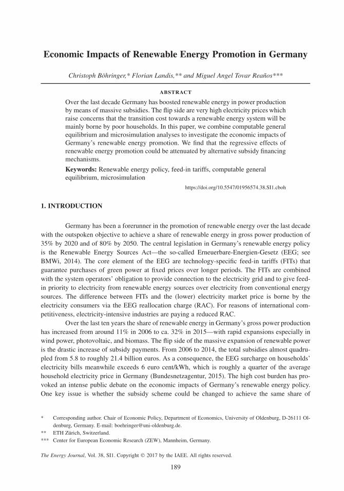
We employ separable nested constant-elasticity-of-substitution (CES) cost functions tocharacterise price-responsive trade-offs across inputs in production. Figure 1 provides a diagram-matic representation of the nesting structure where we refer to inputs with their input prices.2 Theelasticities of substitution that govern how easy one input can be replaced by another in the pro-duction process are denoted with . In the bottom-level nest, labour and capital are combined in aσvalue-added (VA) nest. VA is then combined with energy in a CES nest that represents a VA–energycomposite. In the top-level nest, a composite of intermediate material inputs trades off against theVA–energy composite at a CES. The composites of energy and material in itself are again CESaggregates of various energy or material inputs. All industries except for fuel resource extractionand electricity generation are characterised by constant-returns-to-scale production functions.



Figure 1: Cost function in production

3. For instance, our approach cannot reflect that a renewable technology such as solar may be a substitute for gas at lowsolar production levels, while the two become complements at higher levels of solar power generation.

In the production of fossil fuels, all inputs, except for the sector-specific fossil fuel resource,are aggregated in fixed proportions. This aggregate trades off with the sector-specific fossil fuelresource at a constant elasticity of substitution.

Given the paramount importance of the electricity sector with respect to the promotion ofrenewable power generation we distinguish discrete generation technologies that produce electricityby combining technology-specific capital with inputs of labour, fuel, and materials. Electricityoutput from different technologies is treated as a homogeneous good. For each technology, powergeneration takes place with decreasing returns to scale and responds to changes in electricity pricesaccording to technology-specific supply elasticities (see Rutherford, 2002, for details on the cali-bration technique). In addition, lower and upper bounds on production capacities can provide ex-plicit limits to the decline and the expansion of technologies. While our activity analysis approachprovides policy-relevant details on individual power generation technologies (compared to the con-ventional aggregate top-down characterisation of production), it must be seen as crude approxi-mation of real-world power production.3

Fossil fuel resources and generation capacity to power technologies are treated as specificcapital in fixed supply, whereas capital otherwise is assumed to be perfectly mobile across sectors;likewise labour can move freely across sectors. Firms operate in perfectly competitive markets andmaximise their profits by selling their products at a price equal to marginal cost.

Preferences and household behaviour. Final consumption demand is determined by a rep-resentative agent who maximises welfare subject to a budget constraint with fixed savings whichdetermines investment demand. The representative household receives income from net factor earn-ings and government transfers. The disposable income is then spent across consumption categoriesat given prices subject to CES preferences where the different consumption categories are tradedoff at a constant elasticity of substitution. Each consumption category consists of goods producedby industrial sectors.



4. Our small-open-economy assumption neglects the potential scope of those German industries that are large globalplayers to pass on a fraction of domestic regulatory cost via higher export prices.

Government. The government collects taxes to finance transfers and the provision of apublic good. The public good is produced with commodities purchased at market prices. Across allpolicy simulations the level of public good provision is kept constant in order to assure a meaningfulcross-comparison analysis without the need to trade off private consumption and government (pub-lic) consumption. By default, the equal-yield public good provision is warranted through lump-sumtransfers between the government and households.

International trade. In international trade, Germany is treated as small relative to the worldmarket. That is, we assume that changes in German import and export volumes have no effect onits terms of trade.4 Domestic and foreign products are distinguished by the Armington assumptionof product heterogeneity (Armington, 1969). On the import side, domestic goods and importedgoods of the same variety are combined to a so-called Armington composite that enters intermediateand final demands. On the export side, goods destined for domestic and international markets aretreated as imperfect substitutes, produced subject to a constant elasticity of transformation. Weimpose a constant trade balance with respect to the rest of the world, accounting for an exogenouslyspecified net trade surplus which is warranted through an endogenous real exchange rate.

2.1.2 Data

As is customary in applied general equilibrium analysis, benchmark quantities and prices—together with exogenous elasticities—are used to calibrate the model. They determine the freeparameters of the functional forms that capture production technologies and consumer preferences.

We use the input–output table of the German federal statistical office for the year 2006 asthe central data source for model calibration. The choice of 2006 as the base-year for model cali-bration is motivated by the fact that renewable energy subsidies under the EEG started to becomequite substantial from 2006 onward. The first quadrant of the input–output table reports intermediateinputs for each sector. The second quadrant provides information on final demand components:private and public consumption, investment, inventory changes, and exports. Factor payments tolabour and capital (combined with profits in the row ‘operating surplus’) are included in the thirdquadrant which also reports the inflows of foreign goods and services to each production sector.Output by production sector is linked to consumption by private households in terms of consumptionexpenditure categories through the Z-matrix (the so-called ‘Konsumverflechtungstabelle’). Theelectricity sector is decomposed into discrete power generation technologies according to technol-ogy-specific production shares provided by AG Energiebilanzen e.V. (2016) and input cost sharesprovided by Wissel et al. (2008).

Elasticities of substitution for the input structure sketched in Figure 1 are chosen in ac-cordance to empirical estimates by Koesler and Schymura (2012) and Steinbuks and Narayanan(2015). The elasticities of substitution in fossil fuel sectors are calibrated to match exogenousestimates of fossil fuel supply elasticities (Graham et al., 1999; Krichene, 2002). The price elastic-ities of electricity supply by technologies are calibrated to match the changes in power generationshares across technologies following the massive subsidies to renewables over the period between2006 and 2014 (see scenario DIFFRACX in Section 3).



Table 1: Overview of sectors, consumption categories, and power generation technologies

SectorsPrimary and secondary energy Crude oil (cru)†, Coal mining (coa)‡, Natural gas (gas)*

Electricity supply (ele), Coke and mineral oil products (oil)*,Electricity-intensive and trade-exposed Food production (fod), Textiles (tex), Leather (lea),

Timber (tim), Paper (pap), Paper products (ppp),Chemicals (chm), Rubber (rub), Plastics (syn),Glass (gla), Stoneware (sto),Iron and wrought material from iron (cir),Non-iron metals and wrought material from such metals (nim),Foundry products (fnd), Metal products (mpr),Research and development (red),

Remaining industries Not electricity-intensive and trade-exposed (NEITE),Electricity-intensive and not trade-exposed (EINTE),Not electricity-intensive and not trade-exposed (NEINTE),

Consumption categories Food, Housing, Electricity, Heating, Transport,Education and leisure, Other non-durable goods and services,Durables

Electricity generation technologies Coal, Nuclear, Gas, Hydro, Solar, Wind, Biomass

† cru is electricity-intensive and trade-exposed.‡ coa is grouped with EINTE in the results section.* gas and oil are grouped with NEINTE in the results section.

Table 1 provides an overview of sectors, consumption categories and power generationtechnologies that are explicitly represented in our CGE model. As to sectors, we include all primary(coal, crude oil, gas) and secondary (refined oil, electricity) energy carriers that are present in theGerman IO table. The distinction of energy carriers is relevant for capturing inter-fuel substitutionpossibilities in production and consumption. As we want to highlight the effects of RAC exemptionson electricity-intensive and trade-exposed sectors, we refrain from aggregating sectors from the IOtable that display above-average electricity-intensity (electricity expenditures per sales revenue) andtrade-exposure (value share of exports in total sales). The remainder is aggregated in three compositesectors: electricity-intensive and not trade-exposed (EINTE), not electricity-intensive and trade-exposed (NEITE), not electricity-intensive and not trade-exposed (NEINTE).

As to consumption categories, we follow Nichele and Robin (1995) for the representationof expenditure groups in the demand system where energy-intensive goods such as electricity,heating, and transport are singled out. Our specification avoids multiple zeros in the reported cate-gories which would require more complex estimation methods. For power technologies, the modeldistinguishes between four types of renewable power that receive different feed-in tariffs: hydropower, wind power, photovoltaics, and biomass. The model also considers coal, gas, and nuclearas major conventional power generation technologies.

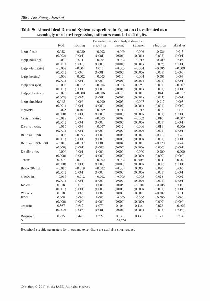
2.2 Microsimulation (MS) model

The core of the microsimulation model is the AIDS established by Deaton and Muellbauer(1980). Data from income and expenditure surveys is used to estimate the AIDS which then drivesdemand responses of households in the MS model. As is the case for the representative householdin the CGE model, each household in the MS model is represented by its factor endowments from



5. The estimated parameters follow the standard constraints for homogeneity and .α = 1 γ = γ = β = 0∑ ∑ ∑ ∑i ij ij ii i j i

6. For the econometric estimation, we follow standard practice by approximating the price index P using the Stone index(Deaton and Muellbauer, 1980).

which it receives income, its savings decision, and its spending of disposable income across con-sumption categories.

2.2.1 Model summary

The AIDS assumes an expenditure function which is homogeneous of degree onere(p,u)in prices.5 Applying Shephard’s lemma yields the following system of budget shares:

mh = α + γ log p + β log , (1)∑i i ij j i Pj

where , , denote expenditure shares for commodities , commodity prices and total expen-h p m ii i

ditures. is a price index given byP

1log P = α + α log p + γ log p log p , (2)∑ ∑∑0 i i i,j i j2i i j

Our econometric estimation is based on data for 128,245 households. In order to captureheterogeneity in consumption behaviour, the parameters and are allowed to differ across sevenγ βij i

household groups (see Blundell et al., 1993). These groups, which account for household size andage of the head of household, are as follows: single + 65 (above 65 years), single no children,single with children, 2 adults + 65 no children, 2 adults no children, 2 adults one child, 2 adultstwo children.

The system is then estimated employing the Seemingly Unrelated Regression (Zellner,1962). The estimated parameters related to price and income changes are statistical significant (seeTable 9 in Appendix 6.1).6 Changes in commodity prices and income simulated by the CGE modelare passed to the AIDS system through the terms and . The equilibrium prices are used top mi

estimate as defined in equation (2). These values are then used to compute our welfare metric ofPequivalent variation (EV) which following Creedy and Sleeman (2006), is derived as follows:

βi¯EV P p mi= exp ∏ log –1, (3)� � � � � � ��m m p Pi i

where and are the reference price levels and total expenditure. Moreover, we use Atkinson’sp mi

index (Atkinson, 1970) to quantify the trade-off between efficiency and equity (e.g., mean equiv-alent income and its distribution across households), which is defined as follows:

(Y + EV ) hsize∑ �no-policy,h h hhSocial Welfare = � (1– A�),

hsize∑ hh (4)14444244443Mean equivalent income (MEI)



7. Education and leisure, Transport, Other non-durable goods and services, Durables

where is total household expenditure in the no-policy situation (in our case the base-yearYno-policy

equilibrium), hsize is household size, and is Atkinson’s inequality index at a given level of theA�

inequality aversion parameter (see e.g. King, 1983).�

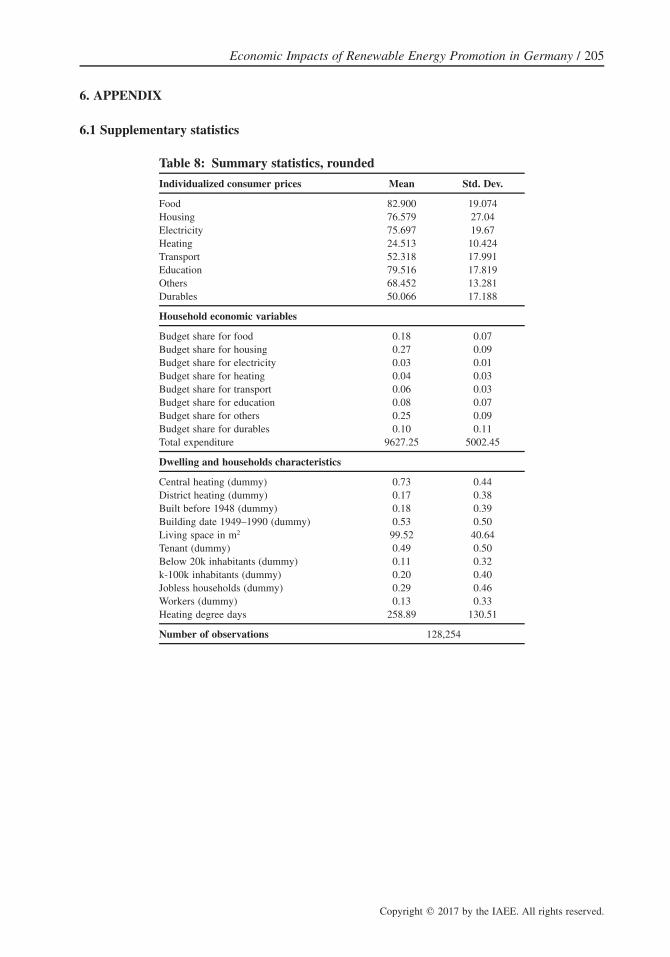
2.2.2 Data

The AIDS is based on the German income and expenditure survey (the so-called Einkom-mens- und Verbrauchsstichprobe—EVS), which provides information on expenditure across dif-ferent commodities, income, and other socioeconomic variables. The survey is carried out everyfive years. We use the waves 1993, 1998, 2003, 2008 and 2013 for the econometric estimation andonly the wave 2008 (closest to 2006, the year the input–output table for the CGE model refers to)for the microsimulation exercise. Thus, the econometric estimation is based on 128 245 observationsand the MS model includes 34 506 households. Regarding prices, we use Lewbel’s (1989) meth-odology to obtain household-specific prices by combining the micro data and prices reported bythe German Statistical Office. Table 8 in the Appendix provides mean and standard deviation ofthe variables used in the estimation.

2.3 Linkage of CGE and MS models

The coupling approach follows the decomposition method by Rutherford and Tarr (2008).It uses the CGE model which represents households by one single representative household in orderto evaluate impacts of given policies on market prices for consumer goods and production factors.The MS model then takes these prices as given and calculates first household income and thenhousehold consumption at the given prices. The representative household in the CGE model is thenrecalibrated such that it reproduces aggregate consumption according to the MS model at presentprices. This creates new imbalances in the markets for the consumption goods. By repeatedlyresolving the top-down model and re-evaluating the MS model at new market prices the two modelsconverge towards an overall consistent solution of the integrated CGE–MS model system. Thus,the coupled model produces the same results as would a stand-alone CGE model with all thehouseholds now included in the MS model. The combined CGE–MS approach has the advantagethat the two parts of the model remain numerically tractable for large numbers of households andthereby also makes the numerical solution process less time-consuming.

In order to achieve a tight link between the CGE model and the MS model, we need theaggregate incomes and consumption demands of households in the MS model to match the corre-sponding numbers in the CGE model. The survey data used in the MS model comes with statisticalweights, which indicate how many of Germany’s actual households are represented by one house-hold in the survey. The aggregate consumption and income from the survey data in general, however,does not coincide with national accounts in the Z-matrix. We scale up households’ total expenditurefrom the survey to match total household expenditure according to national accounts. For imple-menting the AIDS, it is imperative that we leave expenditure shares as they are in the survey. Thus,differences in national household expenditure on a commodity basis must be adjusted for in theCGE model. We do so by shifting the residual demands to government consumption. Thus, forconsumption categories where a positive amount of consumption is transferred to the government,7

overall market demand is less responsive to price changes than in a situation where all of con-



Table 2: Scenario overview

differentiated RAC uniform RAC VA tax

uniform FIT UNIRACX UNIRAC UNIVATdifferentiated FIT DIFFRACX DIFFRAC DIFFVAT

8. Food, Electricity, Heating, Housing9. In 2014 the average FITs amounted to roughly 34 euro cents per kWh for photovoltaics, 20 euro cents per kWh for

biofuels, and 13 euro cents per kWh for wind power.10. Complementary analysis would involve an explicit dynamic perspective assessing different unwinding scenarios

with FITs and subsidy payments being shifted over time from DIFFRACX to the alternative schemes listed in Table 2.

sumption according to the IO table was subject to household’s demand response. For consumptioncategories, where the government has to supply consumption categories for household demand thatis beyond what is supplied according to the IO table,8 demand is more responsive.

On the income side, we scale capital and labour income in the MS model uniformly acrossall households. Lacking information about savings from the survey, we distribute saving decisionsamong households in proportion to their capital income. The residual between expenditure, savings,and factor income is allocated to government transfers.

3. SCENARIOS

The reference scenario for our economic impact assessment is established by the designof Germany’s renewable promotion policy as mandated under the EEG: (i) there are FITs that varysubstantially across renewable technologies, and (ii) the difference between the electricity marketprice and the technology-specific FITs is financed by a RAC across electricity consumers withelectricity-intensive industries paying only a fraction of the nominal RAC. In our simulation analysiswe investigate how the cost magnitude and cost distribution of renewable promotion policy changeas we change the EEG prescriptions along two dimensions. The first dimension refers to the cost-effectiveness of renewable subsidies. Instead of differentiated FITs,9 one could grant uniform sub-sidies in order to equalise marginal cost of renewable expansion across technologies. The seconddimension reflects concerns on distributional impacts of the RAC: to avoid discrimination acrosselectricity consumers, one would at least postulate electricity-intensive sectors to pay the full RAC;alternatively, one might abolish the RAC and switch to a financing of the renewable energy subsidiesby increasing value-added taxes.

We distinguish renewable promotion policy scenarios with respect to tariff design [differ-entiated (labelled DIFF-) versus uniform (labelled UNI-)] and the financing of subsidy payments(RAC with exemptions (labelled -RACX), RAC without exemptions (labelled -RAC), or VA tax(labelled -VAT)). In total, we obtain six scenarios with acronyms as provided in Table 2. Note thatscenario DIFFRACX most closely reflects the current design of the EEG and represents the referenceagainst which we try to find improvements. Given that Germany cannot unwind its EEG policy inthe past, our analysis of alternative policy options is retrospective. However, our insights into themagnitude and distribution of economic adjustment cost for alternative regulatory designs may spurthe German discussion on future reforms regarding the future design of FITs and the payments forsubsidies.10



11. Fischer (2010) shows that promotion of renewable energy sources in electricity generation can have ambiguouseffects on electricity prices depending on the price elasticities of supply across technologies.

12. The EEG allows firms that use more than 1 GWh of electric power per annum and spend more on electricity than14% of their value-added to apply for reduced rates. Annual electricity demand beyond 1 GWh is then charged a lowerRAC with further reductions for demand beyond 10 GWh and 100 GWh.

13. See Appendix 6.2 for details.

Across all renewable promotion scenarios, we keep the electricity generation from renew-able energy sources at the level of scenario DIFFRACX to accommodate a coherent cost-effective-ness analysis of alternative policy designs. The economic impacts of renewable promotion aremeasured against a no-policy scenario which we take as the 2006 base-year equilibrium before themassive penetration of renewable energy into the power system started.

In our scenario analysis, we abstain from any other policy regulations—such as the EUETS—but focus solely on the impacts of renewable energy promotion.

4. RESULTS

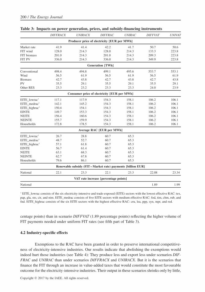
We start the discussion of simulation results with electricity market effects. Changes inelectricity prices induced by alternative designs of renewable power promotion constitute a keydriver of economic impacts at the sector level, in particular for electricity-intensive industries. Wethen assess the aggregate macroeconomic cost of policy reforms from the perspective of a repre-sentative agent neglecting any details and concerns on cost distribution. Finally, we discuss theincidence of renewable energy promotion policies across different households.

If not mentioned otherwise, all results are reported in percentage change from the no-policy benchmark.

4.1 Electricity market effects

Table 3 shows the impacts across our policy scenarios on electricity generation, electricityprices, and the policy instruments to finance renewable power. Overall power generation changeslittle across the different scenarios that finance the FIT with a RAC. Only if the FIT is financed bya value-added tax, does electricity generation increase due to a demand-side effect from lowerconsumer prices. Consumer prices of electricity vary considerably in scenarios in which RAC hasexemptions (UNIRACX and DIFFRACX). The average RAC rate that different electricity consumerspay are given in the fourth section of Table 3. The total volume of RAC payments necessary forreaching the targeted renewable energy sources (RES) generation in electricity generation is givenin the fifth section and increases somewhat for scenarios in which the FIT is uniform.11 Withoutpreferential treatment of electricity-intensive industries (scenarios DIFFRAC and UNIRAC), allconsumer groups face a uniform RAC rate. The RAC is applied to total electricity consumptionand finances the difference between FIT payments and the (lower) market value of RES electricitygeneration. With differentiated RAC rates (scenarios DIFFRACX and UNIRACX), electricity-inten-sive industries pay a lower rate.12 We use base-year statistics to determine for each industry in ourdataset what fraction of electricity demand applies for the reduced rate which then yields the ef-fective adjustment factor to the nominal RAC rate.13 The nominal RAC rate (which applies forhousehold consumption and industries that do not qualify for exemptions) then must increase tomake up for lower effective RAC rates of industries with exemptions. The increase in the value-added tax that is necessary for financing the FIT again is higher in scenario UNIVAT (1.99 per-



Table 3: Impacts on power generation, prices, and subsidy-financing instruments

DIFFRACX UNIRACX DIFFRAC UNIRAC DIFFVAT UNIVAT

Producer price of electricity [EUR per MWh]

Market rate 41.9 41.4 42.2 41.7 50.7 50.6FIT wind 128.0 214.3 128.0 214.3 133.3 223.8FIT biomass 201.0 214.3 201.0 214.3 209.3 223.8FIT PV 336.0 214.3 336.0 214.3 349.9 223.8

Generation [TWh]

Conventional 498.4 494.8 499.1 495.6 553.7 553.1Wind 56.5 61.9 56.5 61.9 56.5 61.9Biomass 42.7 43.8 42.7 43.8 42.7 43.8PV 35.5 29.1 35.5 29.1 35.5 29.1Other RES 23.3 23.2 23.3 23.3 24.0 23.9

Consumer price of electricity [EUR per MWh]

EITE_lowrac† 117.1 117.9 154.3 158.1 106.2 106.1EITE_medrac† 142.1 145.2 154.3 158.1 106.2 106.1EITE_highrac† 150.4 154.1 154.3 158.1 106.2 106.1EINTE 149.7 153.3 154.3 158.1 106.2 106.1NEITE 156.4 160.6 154.3 158.1 106.2 106.1NEINTE 155.7 159.9 154.3 158.1 106.2 106.1Households 172.8 178.5 154.3 158.1 106.2 106.1

Average RAC [EUR per MWh]

EITE_lowrac† 26.7 28.8 60.7 65.3EITE_medrac† 48.7 52.7 60.7 65.3EITE_highrac† 57.1 61.8 60.7 65.3EINTE 56.7 61.4 60.7 65.3NEITE 63.1 68.3 60.7 65.3NEINTE 62.7 67.8 60.7 65.3Households 79.6 86.1 60.7 65.3

Renewable subsidy (FIT–Market rate) payments [billion EUR]

National 22.1 23.3 22.1 23.3 22.08 23.34

VAT rate increase [percentage points]

National 1.89 1.99

† EITE_lowrac consists of the six electricity-intensive and trade-exposed (EITE) sectors with the lowest effective RAC: tex,pap, gla, sto, cir, and nim. EITE_medrac consists of five EITE sectors with medium effective RAC: fod, tim, chm, rub, andfnd. EITE_highrac consists of the six EITE sectors with the highest effective RAC: cru, lea, ppp, syn, mpr, and red.

centage points) than in scenario DIFFVAT (1.89 percentage points) reflecting the higher volume ofFIT payments needed under uniform FIT rates (see fifth part of Table 3).

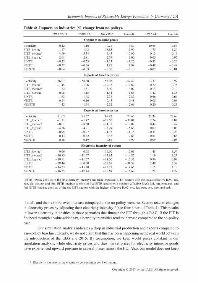
4.2 Industry-specific effects

Exemptions to the RAC have been granted in order to preserve international competitive-ness of electricity-intensive industries. Our results indicate that abolishing the exemptions wouldindeed hurt those industries (see Table 4): They produce less and export less under scenarios DIF-FRAC and UNIRAC than under scenarios DIFFRACX and UNIRACX. But it is the scenarios thatfinance the FIT through an increase in value-added taxes that would constitute the most favourableoutcome for the electricity-intensive industries. Their output in these scenarios shrinks only by little,



Table 4: Impacts on industries (% change from no-policy).


Output at baseline prices

Electricity –0.42 –1.10 –0.21 –0.87 10.65 10.54EITE_lowrac† –1.17 –1.43 –18.85 –19.90 1.75 1.80EITE_medrac† –4.99 –5.34 –7.45 –7.90 0.13 0.16EITE_highrac† –2.61 –2.81 –2.79 –3.00 –0.05 –0.05EINTE –0.53 –0.53 –1.23 –1.26 –0.32 –0.29NEITE –0.37 –0.36 1.87 1.99 –0.48 –0.49NEINTE –0.04 –0.03 –0.10 –0.10 –0.02 –0.01

Imports at baseline prices

Electricity –56.07 –58.60 –55.03 –57.49 –3.37 –3.97EITE_lowrac† –1.45 –1.66 –10.32 –10.82 0.72 0.75EITE_medrac† –1.72 –1.81 –3.90 –4.07 –0.14 –0.10EITE_highrac† –0.95 –1.15 –1.44 –1.66 1.42 1.38EINTE –1.63 –1.68 –2.78 –2.87 –0.66 –0.64NEITE –0.14 –0.16 –0.45 –0.48 0.05 0.06NEINTE –1.42 –1.54 –2.52 –2.69 0.20 0.23

Exports at baseline prices

Electricity 71.63 75.57 69.92 73.63 22.34 22.69EITE_lowrac† –1.11 –1.42 –28.50 –30.01 2.74 2.82EITE_medrac† –8.01 –8.60 –11.37 –12.09 0.44 0.47EITE_highrac† –4.56 –4.91 –5.29 –5.68 0.02 0.03EINTE –0.95 –0.97 –1.13 –1.15 –0.31 –0.28NEITE –0.43 –0.42 2.47 2.63 –0.61 –0.63NEINTE 0.18 0.19 0.86 0.90 0.09 0.08

Electricity intensity of output

EITE_lowrac† –0.06 –0.08 –16.60 –17.63 1.48 1.54EITE_medrac† –10.85 –11.67 –13.95 –14.82 1.19 1.23EITE_highrac† –10.91 –11.67 –11.60 –12.32 0.96 0.99EINTE –28.46 –30.30 –29.65 –31.38 2.48 2.58NEITE –14.23 –15.20 –13.77 –14.65 1.15 1.19NEINTE –16.35 –17.44 –15.69 –16.67 1.21 1.27

† EITE_lowrac consists of the six electricity-intensive and trade-exposed (EITE) sectors with the lowest effective RAC: tex,pap, gla, sto, cir, and nim. EITE_medrac consists of five EITE sectors with medium effective RAC: fod, tim, chm, rub, andfnd. EITE_highrac consists of the six EITE sectors with the highest effective RAC: cru, lea, ppp, syn, mpr, and red.

14. Electricity intensity is the electricity consumption per € of output.

if at all, and their exports even increase compared to the no-policy scenario. Sectors react to changesin electricity prices by adjusting their electricity intensity14 (see fourth part of Table 4). This resultsin lower electricity intensities in those scenarios that finance the FIT through a RAC. If the FIT isfinanced through a value-added tax, electricity intensities tend to increase compared to the no-policycase.

Our simulation analysis indicates a drop in industrial production and exports compared toa no-policy baseline. Clearly, we do not claim that this has been happening in the real world betweenthe introduction of the EEG and 2015. By assumption, we keep world prices constant in oursimulation analysis, while electricity prices and thus market prices for electricity intensive goodshave experienced upward pressure in several places across the EU. Also, our model does not keep



Table 5: Impacts on consumer and factor prices (% change from no-policy)


Consumption goods

Food 0.24 0.26 0.18 0.20 1.93 2.04Education and leisure 0.03 0.02 –0.15 –0.16 1.94 2.05Electricity 58.48 63.63 41.51 44.97 –0.76 –0.75Heating –1.07 –1.11 –1.13 –1.16 1.75 1.87Housing –0.24 –0.26 –0.51 –0.54 1.94 2.06Transport –0.11 –0.12 –0.31 –0.32 1.94 2.05Other goods and services –0.16 –0.17 –0.38 –0.40 1.94 2.05Durables 0.08 0.09 –0.08 –0.08 1.95 2.06

Income factors

Wages –0.68 –0.76 –0.83 –0.91 0.23 0.22Rents on

capital –0.44 –0.45 –0.86 –0.89 –0.15 –0.13resources –13.73 –14.40 –16.79 –17.59 –1.75 –1.69technologies 70.87 81.48 71.66 82.33 105.42 118.25average 0.59 0.75 0.17 0.30 1.50 1.72

15. Equivalent income denotes the amount of money that households would need to afford a scenario’s utility level ofconsumption at prices of the no-policy scenario.

track of which power utilities own which assets and thus is not able to capture the financial distressthat particular German power companies have gone through over the last decade.

4.3 Macroeconomic cost

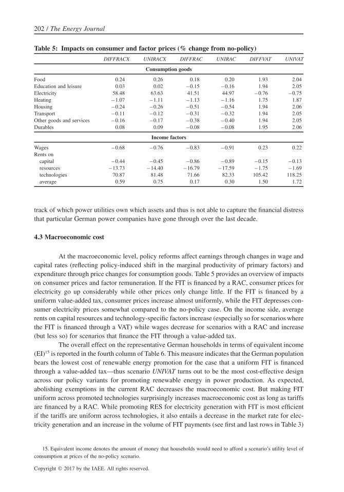
At the macroeconomic level, policy reforms affect earnings through changes in wage andcapital rates (reflecting policy-induced shift in the marginal productivity of primary factors) andexpenditure through price changes for consumption goods. Table 5 provides an overview of impactson consumer prices and factor remuneration. If the FIT is financed by a RAC, consumer prices forelectricity go up considerably while other prices only change little. If the FIT is financed by auniform value-added tax, consumer prices increase almost uniformly, while the FIT depresses con-sumer electricity prices somewhat compared to the no-policy case. On the income side, averagerents on capital resources and technology-specific factors increase (especially so for scenarios wherethe FIT is financed through a VAT) while wages decrease for scenarios with a RAC and increase(but less so) for scenarios that finance the FIT through a value-added tax.

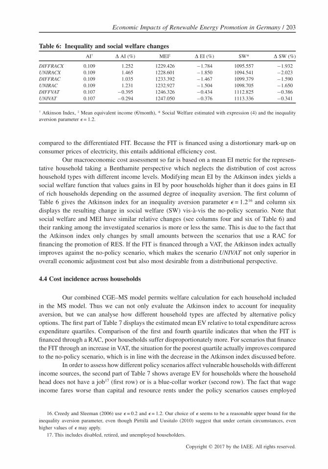
The overall effect on the representative German households in terms of equivalent income(EI)15 is reported in the fourth column of Table 6. This measure indicates that the German populationbears the lowest cost of renewable energy promotion for the case that a uniform FIT is financedthrough a value-added tax—thus scenario UNIVAT turns out to be the most cost-effective designacross our policy variants for promoting renewable energy in power production. As expected,abolishing exemptions in the current RAC decreases the macroeconomic cost. But making FITuniform across promoted technologies surprisingly increases macroeconomic cost as long as tariffsare financed by a RAC. While promoting RES for electricity generation with FIT is most efficientif the tariffs are uniform across technologies, it also entails a decrease in the market rate for elec-tricity generation and an increase in the volume of FIT payments (see first and last rows in Table 3)



Table 6: Inequality and social welfare changes

AI† D AI (%) MEI‡ D EI (%) SW* D SW (%)

DIFFRACX 0.109 1.252 1229.426 –1.784 1095.557 –1.932UNIRACX 0.109 1.465 1228.601 –1.850 1094.541 –2.023DIFFRAC 0.109 1.035 1233.392 –1.467 1099.379 –1.590UNIRAC 0.109 1.231 1232.927 –1.504 1098.705 –1.650DIFFVAT 0.107 –0.395 1246.326 –0.434 1112.825 –0.386UNIVAT 0.107 –0.294 1247.050 –0.376 1113.336 –0.341

† Atkinson Index, ‡ Mean equivalent income (€/month), * Social Welfare estimated with expression (4) and the inequalityaversion parameter � = 1.2.

16. Creedy and Sleeman (2006) use and . Our choice of seems to be a reasonable upper bound for the� = 0.2 � = 1.2 �

inequality aversion parameter, even though Pirttila and Uusitalo (2010) suggest that under certain circumstances, evenhigher values of may apply.�

17. This includes disabled, retired, and unemployed householders.

compared to the differentiated FIT. Because the FIT is financed using a distortionary mark-up onconsumer prices of electricity, this entails additional efficiency cost.

Our macroeconomic cost assessment so far is based on a mean EI metric for the represen-tative household taking a Benthamite perspective which neglects the distribution of cost acrosshousehold types with different income levels. Modifying mean EI by the Atkinson index yields asocial welfare function that values gains in EI by poor households higher than it does gains in EIof rich households depending on the assumed degree of inequality aversion. The first column ofTable 6 gives the Atkinson index for an inequality aversion parameter 16 and column six� = 1.2displays the resulting change in social welfare (SW) vis-a-vis the no-policy scenario. Note thatsocial welfare and MEI have similar relative changes (see columns four and six of Table 6) andtheir ranking among the investigated scenarios is more or less the same. This is due to the fact thatthe Atkinson index only changes by small amounts between the scenarios that use a RAC forfinancing the promotion of RES. If the FIT is financed through a VAT, the Atkinson index actuallyimproves against the no-policy scenario, which makes the scenario UNIVAT not only superior inoverall economic adjustment cost but also most desirable from a distributional perspective.

4.4 Cost incidence across households

Our combined CGE–MS model permits welfare calculation for each household includedin the MS model. Thus we can not only evaluate the Atkinson index to account for inequalityaversion, but we can analyse how different household types are affected by alternative policyoptions. The first part of Table 7 displays the estimated mean EV relative to total expenditure acrossexpenditure quartiles. Comparison of the first and fourth quartile indicates that when the FIT isfinanced through a RAC, poor households suffer disproportionately more. For scenarios that financethe FIT through an increase in VAT, the situation for the poorest quartile actually improves comparedto the no-policy scenario, which is in line with the decrease in the Atkinson index discussed before.

In order to assess how different policy scenarios affect vulnerable households with differentincome sources, the second part of Table 7 shows average EV for households where the householdhead does not have a job17 (first row) or is a blue-collar worker (second row). The fact that wageincome fares worse than capital and resource rents under the policy scenarios causes employed



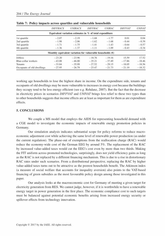
Table 7: Policy impacts across quartiles and vulnerable households


Equivalent variation estimates in % of total expenditure

1st quartile –2.07 –2.19 –1.68 –1.77 0.01 0.042nd quartile –1.98 –2.06 –1.62 –1.68 –0.44 –0.393rd quartile –1.71 –1.75 –1.41 –1.43 –0.64 –0.574th quartile –1.36 –1.37 –1.11 –1.09 –0.43 –0.34

Monthly equivalent variation for vulnerable households (€)

Jobless –23.20 –23.96 –18.76 –19.16 15.59 17.52Blue-collar workers –43.08 –46.00 –35.21 –37.49 –17.86 –18.46Tenants –33.84 –35.99 –27.52 –29.15 –18.05 –18.56Occupants of old dwellings –27.95 –26.79 –23.47 –21.73 –21.19 –18.32

working age households to lose the highest share in income. On the expenditure side, tenants andoccupants of old dwellings may be more vulnerable to increases in energy cost because the buildingsthey occupy tend to be less energy efficient (see e.g. Rehdanz, 2007). But the fact that the decreasein electricity prices in scenarios DIFFVAT and UNIVAT brings less relief to these two types thanto other households suggests that income effects are at least as important for them as are expenditureeffects.

5. CONCLUSIONS

We couple a MS model that employs the AIDS for representing household demand witha CGE model to investigate the economic impacts of renewable energy promotion policies inGermany.

Our simulation analysis indicates substantial scope for policy reforms to reduce macro-economic adjustment cost while achieving the same level of renewable power production (as underthe current regulation). The phase-out of exemptions from the reallocation charge (RAC) wouldreduce the economy-wide cost of the German EEG by around 5%. The replacement of the RACby increased value-added taxes would cut the EEG’s cost even by more than two thirds. Makingthe FIT uniform across promoted technologies, surprisingly, does not yield efficiency gains as longas the RAC is not replaced by a different financing mechanism. This is due to a rise in distortionaryRAC rates under such scenarios. From a distributional perspective, replacing the RAC by highervalue-added taxes turns out to be attractive as the poorest households benefit. The Atkinson index(a measure of social welfare that accounts for inequality aversion) also points to the VAT-basedfinancing of green subsidies as the most favourable policy design among those investigated in thispaper.

Our analysis looks at the macroeconomic cost for Germany of meeting a given target forelectricity generation from RES. We cannot judge, however, if it is worthwhile to have a renewableenergy target in power generation in the first place. The economic compliance cost to such targetsmust be balanced against potential economic benefits arising from increased energy security orspillover effects from technology innovation.



6. APPENDIX

6.1 Supplementary statistics

Table 8: Summary statistics, rounded

Individualized consumer prices Mean Std. Dev.

Food 82.900 19.074Housing 76.579 27.04Electricity 75.697 19.67Heating 24.513 10.424Transport 52.318 17.991Education 79.516 17.819Others 68.452 13.281Durables 50.066 17.188

Household economic variables

Budget share for food 0.18 0.07Budget share for housing 0.27 0.09Budget share for electricity 0.03 0.01Budget share for heating 0.04 0.03Budget share for transport 0.06 0.03Budget share for education 0.08 0.07Budget share for others 0.25 0.09Budget share for durables 0.10 0.11Total expenditure 9627.25 5002.45

Dwelling and households characteristics

Central heating (dummy) 0.73 0.44District heating (dummy) 0.17 0.38Built before 1948 (dummy) 0.18 0.39Building date 1949–1990 (dummy) 0.53 0.50Living space in m2 99.52 40.64Tenant (dummy) 0.49 0.50Below 20k inhabitants (dummy) 0.11 0.32k-100k inhabitants (dummy) 0.20 0.40Jobless households (dummy) 0.29 0.46Workers (dummy) 0.13 0.33Heating degree days 258.89 130.51

Number of observations 128,254



Table 9: Almost Ideal Demand System as specified in Equation (1), estimated as aseemingly unrelated regression, estimates rounded to 3 digits.

Dependent variable: budget share for . . .food housing electricity heating transport education durables

log(p_food) 0.028 –0.030 –0.002 –0.009 –0.006 –0.026 0.015(0.002) (0.001) (0.001) (0.001) (0.001) (0.002) (0.001)

log(p_housing) –0.030 0.031 –0.004 –0.002 –0.012 –0.000 0.006(0.001) (0.002) (0.000) (0.001) (0.001) (0.002) (0.001)

log(p_electricity) –0.002 –0.004 0.015 –0.003 –0.004 –0.006 –0.000(0.001) (0.000) (0.001) (0.000) (0.000) (0.001) (0.000)

log(p_heating) –0.009 –0.002 –0.003 0.010 –0.004 –0.001 0.003(0.001) (0.001) (0.000) (0.001) (0.001) (0.001) (0.001)

log(p_transport) –0.006 –0.012 –0.004 –0.004 0.025 0.001 –0.007(0.001) (0.001) (0.000) (0.001) (0.001) (0.001) (0.001)

log(p_education) –0.026 –0.000 –0.006 –0.001 0.001 0.044 –0.017(0.002) (0.002) (0.001) (0.001) (0.001) (0.002) (0.001)

log(p_durables) 0.015 0.006 –0.000 0.003 –0.007 –0.017 0.003(0.001) (0.001) (0.000) (0.001) (0.001) (0.001) (0.002)

log(M/P) –0.025 –0.107 –0.009 –0.013 –0.012 0.002 0.113(0.000) (0.001) (0.000) (0.000) (0.000) (0.001) (0.001)

Central heating –0.018 0.009 –0.005 0.009 –0.002 0.010 –0.007(0.001) (0.001) (0.000) (0.000) (0.000) (0.001) (0.001)

District heating –0.016 0.007 –0.007 0.012 –0.006 0.011 –0.006(0.001) (0.001) (0.000) (0.000) (0.000) (0.001) (0.001)

Building: 1948 –0.006 –0.053 0.002 0.006 0.002 –0.017 0.049(0.001) (0.001) (0.000) (0.000) (0.000) (0.001) (0.001)

Building:1949-1990 –0.010 –0.037 0.001 0.004 0.001 –0.020 0.044(0.000) (0.001) (0.000) (0.000) (0.000) (0.000) (0.001)

Dwelling size –0.000 0.001 0.000 0.000 –0.000 –0.000 –0.000(0.000) (0.000) (0.000) (0.000) (0.000) (0.000) (0.000)

Tenant 0.007 –0.011 –0.002 –0.002 0.000* 0.004 –0.001(0.000) (0.001) (0.000) (0.000) (0.000) (0.000) (0.001)

Below 20k inh –0.013 –0.019 –0.002 –0.004 0.000 0.020 0.006(0.001) (0.001) (0.000) (0.000) (0.000) (0.001) (0.001)

k-100k inh –0.015 –0.012 –0.002 –0.006 –0.003 0.028 0.002(0.001) (0.001) (0.000) (0.000) (0.000) (0.001) (0.001)

Jobless 0.018 0.013 0.003 0.005 –0.010 –0.006 0.000(0.001) (0.001) (0.000) (0.000) (0.000) (0.001) (0.001)

Workers 0.018 0.005 0.002 0.003 0.002 –0.009 0.011HDD 0.000 0.000 0.000 –0.000 –0.000 –0.000 0.000

(0.000) (0.000) (0.000) (0.000) (0.000) (0.000) (0.000)constant 0.367 0.652 0.070 0.106 0.136 0.078 –0.405

(0.002) (0.003) (0.001) (0.001) (0.001) (0.003) (0.004)

R-squared 0.275 0.443 0.222 0.139 0.137 0.171 0.214N 128,254

Household specific parameters for prices and expenditure are available upon request.



18. Compare to Mayer and Burger (2014) available at https://www.ise.fraunhofer.de/de/downloads/pdf-files/data-nivc-/kurzstudie-zur-historischen-entwicklung-der-eeg-umlage.pdf

6.2 Derivation of RAC rates

We assume for the share of electricity demand getting exemptions from RAC andsel = 0.2for the share of RAC payed for exempted electricity demand.18 We computesracx = 0.015 rracx

to be

All breaks from RAC sracx 1– selrracx: = = sel ⋅ 1– .� �nominal RAC rate ⋅German electricity demand sel 1– sracx

We define as sector ’s ratio between electricity demand and value-added and argue thateva i di ele,i

eva –0.14ierf ⋅ dele,i� �0.10sre =i eva –0.14jerf ⋅ d∑ ele,jj � �0.10

is a useful assumption about the share of national RAC exemptions going to sector . , theRACi li

difference between the nominal RAC rate and the average effective RAC rate for sector , is thenicomputed as

Effective RAC rate for sector iRACl : =i Nominal RAC rate

Exempt electricity demand of sector i= 1–

Total electricity demand of sector i

sre ⋅ rracx ⋅ d∑i ele,gg= 1– ,dele,i

if index covers all economic agents that demand electricity in Germany.g

ACKNOWLEDGEMENTS

Miguel A. Tovar is grateful for financial support of the German Ministry of Education andResearch (BMBF) under grant 01UT1411A (“Integrierte Analyse einer grunen Transformation”).

Christoph Bohringer is grateful for support from Stiftung Mercator (ZentraClim).Florian Landis is grateful for financial support by the Swiss Commission for Technology

and Innovation (CTI) through the Swiss Competence Center for Energy Research, “CompetenceCenter for Research in Energy, Society and Transition” (SCCER-CREST).

REFERENCES

AG Energiebilanzen e.V. (2016). Bruttostromerzeugung in Deutschland ab 1990 nach Energietragern.Armington, P. S. (1969). A Theory of Demand for Products Distinguished by Place of Production. Staff Papers (International

Monetary Fund), 16(1):159–178. https://doi.org/10.2307/3866403.



Atkinson, A. B. (1970). On the measurement of inequality. Journal of Economic Theory, 2(3):244–263. https://doi.org/10.1016/0022-0531(70)90039-6.

Bohringer, C. (1998). The synthesis of bottom-up and top-down in energy policy modeling. Energy Economics, 20(3):233–248. https://doi.org/10.1016/S0140-9883(97)00015-7.

Bohringer, C., s. Boeters, and M. Feil (2005). Taxation and unemployment: an applied general equilibrium approach.Economic Modelling, 22(1):81–108. https://doi.org/10.1016/j.econmod.2004.05.002.

Bohringer, C., A. Loschel, U. Moslener, and T. F. Rutherford (2009). EU climate policy up to 2020: An economic impactassessment. Energy Economics, 31, Supplement 2:S295–S305. https://doi.org/10.1016/j.eneco.2009.09.009.

Bohringer, C. and K. E. Rosendahl (2010). Green promotes the dirtiest: on the interaction between black and green quotasin energy markets. Journal of Regulatory Economics, 37(3):316–325. https://doi.org/10.1007/s11149-010-9116-1.

Bohringer, C. and T. F. Rutherford (2008). Combining bottom-up and top-down. Energy Economics, 30(2):574–596. https://doi.org/10.1016/j.eneco.2007.03.004.

Blundell, R., P. Pashardes, and G. Weber (1993). What Do We Learn About Consumer Demand Patterns from Micro Data?American Economic Review, 83(3):570–590.

BMWi (2014). Act on the Development of Renewable Energy Sources (Renewable Energy Sources Act - RES Act 2014).Bundesnetzagentur (2015). EEG in Zahlen 2014.Bundesnetzagentur and Bundeskartellamt (2014). Monitoringbericht 2013. Technical report.Creedy, J. and C. Sleeman (2006). The Distributional Effects of Indirect Taxes: Models and Applications from New Zealand.

Edward Elgar Publishing.Deaton, A. and J. Muellbauer (1980). An almost ideal demand system. The American economic review, 70(3):312–326.Fischer, C. (2010). Renewable Portfolio Standards: When Do They Lower Energy Prices? The Energy Journal, 31(1):101–

119. https://doi.org/10.5547/ISSN0195-6574-EJ-Vol31-No1-5.Frondel, M., N. Ritter, C. M. Schmidt, and C. Vance (2010). Economic impacts from the promotion of renewable energy

technologies: The German experience. Energy Policy, 38(8):4048–4056. https://doi.org/10.1016/j.enpol.2010.03.029.Graham, P., S. Thorpe, and L. Hogan (1999). Non-competitive market behaviour in the international coking coal market.

Energy Economics, 21(3):195–212. https://doi.org/10.1016/S0140-9883(99)00006-7.Grosche, P. and C. Schroder (2013). On the redistributive effects of Germany’s feed-in tariff. Empirical Economics,

46(4):1339–1383. https://doi.org/10.1007/s00181-013-0728-z.King, M. A. (1983). Welfare analysis of tax reforms using household data. Journal of Public Economics, 21(2):183–214.

https://doi.org/10.1016/0047-2727(83)90049-X.Koesler, S. and M. Schymura (2012). Substitution Elasticities in a CES Production Framework. An Empirical Analysis on

the Basis of Non-Linear Least Squares Estimations. ZEW Discussion Paper 12-007, ZEW, Mannheim.Krichene, N. (2002). World crude oil and natural gas: a demand and supply model. Energy Economics, 24(6):557–576.

https://doi.org/10.1016/S0140-9883(02)00061-0.Lewbel, A. (1989). Identification and Estimation of Equivalence Scales under Weak Separability. The Review of Economic

Studies, 56(2):311–316. https://doi.org/10.2307/2297464.Mayer, J. N. and B. Burger (2014). Kurzstudie zur historischen Entwicklung der EEG-Umlage. Fraunhofer ISE: Freiburg,

Germany.Monopolkommission (2013). Energie 2013: Wettbewerb in Zeiten der Energiewende. Sondergutachten 65, Bonn.Neuhoff, K., S. Bach, J. Diekmann, M. Beznoska, and T. El-Laboudy (2013). Distributional Effects of Energy Transition:

Impacts of Renewable Electricity Support in Germany. Economics of Energy & Environmental Policy, 2(1):41–54. https://doi.org/10.5547/2160-5890.2.1.3.

Nichele, V. and J.-M. Robin (1995). Simulation of indirect tax reforms using pooled micro and macro French data. Journal

of Public Economics, 56(2):225–244. https://doi.org/10.1016/0047-2727(94)01425-N.Pirttila, J. and R. Uusitalo (2010). A ‘Leaky Bucket’ in the Real World: Estimating Inequality Aversion using Survey Data.

Economica, 77(305):60–76. https://doi.org/10.1111/j.1468-0335.2008.00729.x.Rehdanz, K. (2007). Determinants of residential space heating expenditures in Germany. Energy Economics, 29(2):167–

182. https://doi.org/10.1016/j.eneco.2006.04.002.Rutherford, T. (2002). Lecture notes on constant elasticity functions.Rutherford, T. F. and D. G. Tarr (2008). Poverty effects of Russia’s WTO accession: Modeling ‘real’ households with

endogenous productivity effects. Journal of International Economics, 75(1):131–150. https://doi.org/10.1016/j.jinteco.2007.09.004.

Statistisches Bundesamt, editor (2011). Jahresgutachten: Sachverstandigenrat zur Begutachtung der gesamtwirtschaftlichen

Entwicklung. 2011/12: Verantwortung fur Europa wahrnehmen. Sachverstandigenrat zur Begutachtung der gesamtwirt-schaftlichen Entwicklung, Statistisches Bundesamt, Wiesbaden.



Steinbuks, J. and B. G. Narayanan (2015). Fossil fuel producing economies have greater potential for industrial interfuelsubstitution. Energy Economics, 47:168–177. https://doi.org/10.1016/j.eneco.2014.11.001.

Wissel, S., S. Rath-Nagel, M. Blesl, U. Fahl, and A. Voß (2008). Stromerzeugungskosten im Vergleich. Arbeitsbericht,Universitat Stuttgart, Institut fur Energiewirtschaft und Rationelle Energieanwendung [IER].

Zellner, A. (1962). An Efficient Method of Estimating Seemingly Unrelated Regressions and Tests for Aggregation Bias.Journal of the American Statistical Association, 57(298):348–368. https://doi.org/10.1080/01621459.1962.10480664.

Copyright of Energy Journal is the property of International Association for EnergyEconomics, Inc. and its content may not be copied or emailed to multiple sites or posted to alistserv without the copyright holder's express written permission. However, users may print,download, or email articles for individual use.

Documents

Economic Impacts of Renewable Energy Promotion …theargeo.org/August/files/Economic Impacts of Renewable...Germany’s renewable energy promotion. We ﬁnd that the regressive effects