CHAPTER 3

Economic Growth

3.1 Introduction

Of all the issues facing development economists, economic growth has tobe one of the most compelling. In Chapter 2, we noted the variety ofgrowth experiences across countries. It is true that all of these numbers,with very few exceptions, were in the single digits, but we also appreciatedthe power of exponential growth. A percentage point added or subtractedcan make the di↵erence between stagnation and prosperity over the periodof a generation. Small wonder, then, that the search for key variables in thegrowth process can be tempting. For precisely this reason, the theory andempirics of economic growth (along with the distribution of that growth)has fired the ambitions and hopes of academic scholars and policy makersalike. I was certainly inspired by Robert Lucas’s Marshall Lectures at theUniversity of Cambridge:

Rates of growth of real per-capita income are diverse, evenover sustained periods. Indian incomes will double every50 years; Korean every 10. An Indian will, on average, betwice as well o↵ as his grandfather; a Korean 32 times.1

I do not see how one can look at figures like these withoutseeing them as representing possibilities. . . The consequencesfor human welfare involved in questions like these aresimply staggering: Once one starts to think about them,it is hard to think about anything else.

1As we have seen, this is no longer true of India and Korea post 1990, but the general point,made at a time when India was growing slowly, is still valid.

58 Economic Growth

Never mind the fact that India has grown at far faster rates since thesewords were penned. The sentiment still makes sense: Lucas captures,more keenly than any other writer, the passion that drives the study ofeconomic growth. We can sense the big payo↵, the possibility of changewith extraordinarily beneficial consequences, if one only knew the exactcombination of circumstances that drives economic growth.

If only one knew. . . , but to expect a single theory about an incrediblycomplicated economic universe to deliver that would be unwise. Yettheories of economic growth do take us some way in understanding thedevelopment process, at least at an aggregate level. This is especially so ifwe supplement the theories with what we know empirically.

3.2 Modern Economic Growth: Basic Features

Economic growth, as the title of Simon Kuznets’ pioneering book [1966]on the subject suggests, is a relatively “modern” phenomenon. Today, wegreet 3% annual rates of per capita growth with approval but no greatsurprise. But throughout most of human history, such growth — or indeedany growth at all — was the exception rather than the rule. In fact, it isn’tfar from the truth to say that modern economic growth was born after theIndustrial Revolution in Britain.

Consider the growth rates of the world’s leaders over the past fourcenturies. During the period 1580–1820 the Netherlands was the leadingindustrial nation; it experienced an average annual growth in real GDPper worker hour2 of roughly 0.2%. The United Kingdom, leader duringthe approximate period 1820–90, experienced an annual growth of 1.2%.That’s (much) faster than the Netherlands, true, but nevertheless a veritabletortoise compared to today’s hares. And since then it’s been the UnitedStates, but from 1890 to the present it has averaged around 2% a year,dropping to more sedate 1.7% over 1990–2011. That is certainly impressive,but it still isn’t what we’ve seen lately: first from Japan and then from EastAsia more generally, and more recently South Asia.

A little calculation suggests that you don’t even have to look at historyto establish the modernity of economic growth. Simply run our trustyformula on doubling times backwards; (Chapter 2, footnote 15). Let’s usewhat by today’s high standards is a pretty moderate number: 3% per year.A country growing at that rate will halve its income every 23 years or so,

2Notice that we are referring here not to growth in per capita GDP as such, but growth inGDP per worker hour, or labor productivity. However, the data suggests that the former islargely driven by the latter.

Economic Growth 59

Country 1850 1930 2010 1930/1850 2010/1930

Austria 1,650 3,586 24,096 2.2 6.7Belgium 1,847 4,979 23,557 2.7 4.7Canada 1,330 4,811 24,941 3.6 5.2Denmark 1,767 5,341 23,513 3.0 4.4Finland 911 2,666 23,290 2.9 8.7France 1,597 4,532 21,477 2.8 4.7Germany 1,428 3,973 20,661 2.8 5.2Japan 681 1,850 21,935 2.7 11.9Netherlands 2,355 5,603 24,303 2.4 4.3Norway 956 3,627 27,987 3.8 7.7Sweden 1,076 4,238 25,306 3.9 6.0Switzerland 2,293 8,492 25,033 3.7 2.9United Kingdom 2,330 5,441 23,777 2.3 4.4United States 1,849 6,213 30,491 3.4 4.9

Simple Average 1,576 4,668 24,312 3.0 5.2

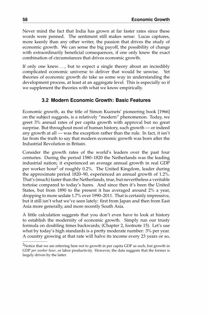
Table 3.1. Per capita GDP (1990 international dollars) inselected OECD countries, 1850–2010.

Source: Maddison [2008] and Bolt and Van Zanden [2013]. First-column Switzerland datafrom 1851.

which means that running back 200 years, that country would have to havean income around 1/350th of what it has today! For the United States, thatwould mean an princely annual income of around $100 per year in 1800.That was most assuredly not the case. And poorer countries extrapolatedbackwards at this rate would vanish.

But of course, this sort of calculation isn’t merely theoretical. You can seethe acceleration, even among now-developed countries, and even if we goright to 2010 (remembering that the first decade of the 21st century hasn’texactly been a bed of roses). Table 3.1 provides a historical glimpse of theperiod 1850–2010, and shows how growth has transformed the world. Thistable displays per capita real GDP (valued in 1990 international dollars)for selected OECD countries in the equally spaced years 1850, 1930, and2010. The penultimate column gives us the ratio of per capita GDP in 1930,at the peak just before the Depression, to its counterpart in 1950. The lastcolumn does the same for the years 2010 and 1930. The numbers are prettystunning. On average (see the last row of the table), GDP per capita in1930 was 3 times the figure for 1850, but the corresponding ratio for theequally long period period between 1930 and 2010 is by 1978 is 5.2! A nearly

60 Economic Growth

Country 1982 1996 2009 Country 1982 1996 2009

Argentina 34.8 28.8 31.6 India 3.7 4.4 7.2Bangladesh 2.4 2.2 3.1 Indonesia 5.7 8.6 9.1Botswana 15.8 22.4 29.1 Malaysia 20.9 28.3 30.5Brazil 27.6 22.3 22.5 Mexico 42.7 29.7 29.8Chile 19.4 27.8 31.3 Nigeria 5.4 4.1 4.8China 2.3 5.8 14.8 Pakistan 5.1 5.5 5.7Cote d’Ivoire 9.9 5.2 3.7 Rwanda 3.3 1.9 2.5Egypt 10.5 10.1 12.3 South Africa 34.8 22.0 22.3Ethiopia 2.3 1.5 2.0 Sri Lanka 6.5 7.3 10.4Ghana 3.3 2.8 3.4 Thailand 9.5 17.1 17.4

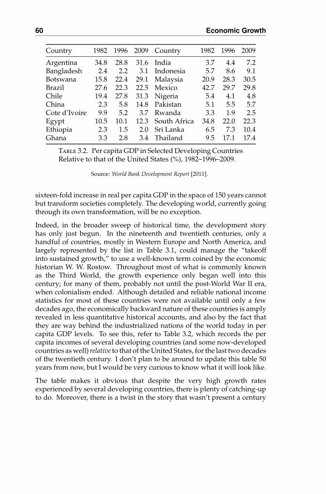
Table 3.2. Per capita GDP in Selected Developing CountriesRelative to that of the United States (%), 1982–1996–2009.

Source: World Bank Development Report [2011].

sixteen-fold increase in real per capita GDP in the space of 150 years cannotbut transform societies completely. The developing world, currently goingthrough its own transformation, will be no exception.

Indeed, in the broader sweep of historical time, the development storyhas only just begun. In the nineteenth and twentieth centuries, only ahandful of countries, mostly in Western Europe and North America, andlargely represented by the list in Table 3.1, could manage the “takeo↵into sustained growth,” to use a well-known term coined by the economichistorian W. W. Rostow. Throughout most of what is commonly knownas the Third World, the growth experience only began well into thiscentury; for many of them, probably not until the post-World War II era,when colonialism ended. Although detailed and reliable national incomestatistics for most of these countries were not available until only a fewdecades ago, the economically backward nature of these countries is amplyrevealed in less quantitative historical accounts, and also by the fact thatthey are way behind the industrialized nations of the world today in percapita GDP levels. To see this, refer to Table 3.2, which records the percapita incomes of several developing countries (and some now-developedcountries as well) relative to that of the United States, for the last two decadesof the twentieth century. I don’t plan to be around to update this table 50years from now, but I would be very curious to know what it will look like.

The table makes it obvious that despite the very high growth ratesexperienced by several developing countries, there is plenty of catching-upto do. Moreover, there is a twist in the story that wasn’t present a century

Economic Growth 61

ago. Then, the now-developed countries grew (although certainly notin perfect unison) in an environment uninhabited by nations of far greatereconomic strength. Today, the story is completely di↵erent. The developingnations not only need to grow, they must grow at rates that far exceedhistorical experience. The developed world already exists, and their accessto economic resources is not only far higher than that of the developingcountries, but the power a↵orded by this access is on display. The urgency ofthe situation is further heightened by the extraordinary flow of informationin the world today. People are increasingly and more quickly aware of newproducts elsewhere and of changes and disparities in standards of livingthe world over. Exponential growth at rates of 2% may well have significantlong-run e↵ects, but they cannot match the parallel growth of humanaspirations, and the increased perception of global inequalities. Perhapsno one country, or group of countries, can be blamed for the emergence ofthese inequalities, but they do exist, and the need for sustained growth isall the more urgent as a result.

3.3 The Beginnings of a Theory

3.3.1 Savings and Investment. In its simplest terms, economic growth isthe result of abstention from current consumption. An economy producesgoods and services. The act of production generates income, which in turnis used to buy these goods and services. Exactly which goods are produceddepends on individual preferences and the distribution of income, but asa broad first pass, the following statement is true: commodity productioncreates income, which creates the demand for those very same commodities.

Let’s go a step further and broadly classify commodities into two groups.We may think of the first group as consumption goods, which are producedfor the express purpose of satisfying human wants and preferences. Themangos you buy at the market, or a tshirt, or an iPad all come under thiscategory. The second group of commodities consists of what we might callcapital goods, which we may think of as commodities that are produced forthe purpose of producing other commodities. A blast furnace, a conveyorbelt, or a screwdriver might come under the second category.3

3It should be clear from our examples that there is an intrinsic ambiguity regarding thisclassification. Although a mango or a blast furnace may be easily classified into its respectivecategory, the same is not true of screwdrivers or an IPad. The correct distinction is betweengoods that generate current consumption and those that produce future consumption, andmany goods embody a little of each.

62 Economic Growth

Firms

Households

Consumption Expenditure

Savings

Investment

Wages, Profits, Rents

Outflow

OutflowInflow

Inflow

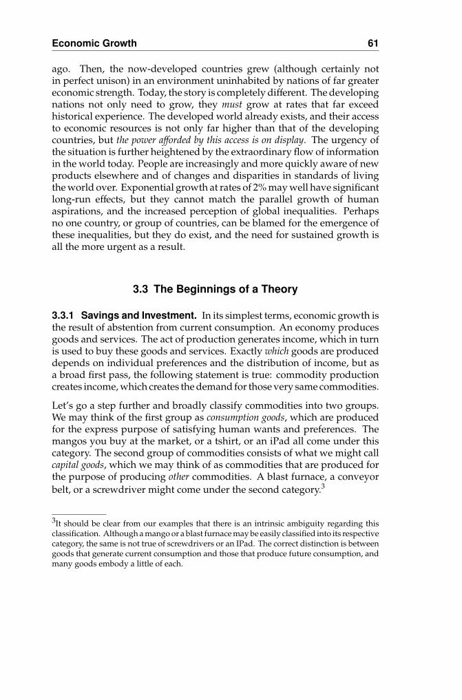
Figure 3.1. Production, consumption, savings, and investment.

Looking around us, it is obvious that the income generated from theproduction of all goods is spent on both consumer goods and capital goods.Typically, households buy consumer goods, whereas firms buy capitalgoods to expand their production or to replace worn-out machinery. Thatimmediately raises a question: if income is paid out to households, andif households spend their income on consumption goods, where does themoney for capital goods come from? How does it all add up?

The answer to this question is simple, although in many senses that weignore here, deceptively so: households save. No doubt some borrowtoo, to finance current consumption, but on the whole, national savings isgenerally positive. All income is not spent on current consumption. Byabstaining from consumption, households make available a pool of funds(via deposits, stock purchases, or undeclared dividends) that firms use tobuy capital goods. This latter purchase is the act of investment. Buyingpower is channeled from savers to investors through banks, individualloans, governments, and stock markets. How these transfers are actuallycarried out is a story in itself. Later chapters will tell some of this story.

Implicit in the story is the idea of macroeconomic balance. Figure 3.1 depictsa circuit diagram with income flowing “out” of firms as they produceand income flowing back “into” firms as they sell. You can visualizesavings as a leakage from the system: the demand for consumption goodsalone falls short of the income that created this demand. Investors fill this

Economic Growth 63

gap by stepping in with their demand for capital goods. Macroeconomicbalance is achieved when this investment demand is at a level that exactlycounterbalances the savings leakage.

By entering a new business, by expanding a current business, or byreplacing worn-out capital, investment creates a market demand for capitalgoods. These goods add to the stock of capital in the economy and endowit, in the future, with an even larger capacity for production, and so aneconomy grows. Note, however, that without the initial availability ofsavings, it would not be possible to invest and there would be no expansion.This is the simple starting point of all of the theory of economic growth.

3.3.2 Inputs, Outputs and the Production Function. At the heart of itall is, of course, production, that most central of all activities that convertsinputs to outputs. It will help — as an organizing device — to introduce theproduction function. It is a simple mathematical description of how variousinputs (such as capital, land, labor, and various raw materials) are combinedto produce outputs. An easy example is one in which just two inputs —capital and labor — combine to produce a single output. Symbolically, wewrite

Y = F(K,L)where K stands for capital, L for labor, Y for output, and F(K,L) ismathematical notation for some function that converts input pairs (K,L)to output Y. A classic instance is the Cobb-Douglas production function, inwhich we write

(3.1) Y = AK↵L�,

for some positive constants A, ↵ and �. The parameter A is a measure ofthe degree of technological proficiency in the economy. The larger it is, thehigher is output for any fixed combination of K and L. The parameters↵ and� capture both the relative importance of each input, as well as whether (andhow much) the marginal returns to each input diminish. It is easy to verifythat if ↵ lies between 0 and 1, then there are diminishing returns to capital:each additional input of capital increases output, but by a progressivelysmaller amount. (The same is true of labor, if � lies between 0 and 1.)Indeed, “diminishing returns to each input” is a reasonable presumption:if more and more of a particular input is added, without changing the amountsof any other input, its marginal e�cacy in producing fresh output should godown.

In contrast, if all inputs — or overall “scale” for short — are increased in thesame proportion, it seems reasonable that output should climb in the sameproportion as well. The argument that makes this sound reasonable is one

64 Economic Growth

of pure replication: if you’ve doubled every input, then it’s like installinga perfect twin of a manufacturing unit: how can output not double? Thattypically starts a discussion with some interesting philosophical twists, butwe will bypass such matters for the moment.4 This phenomenon in whichoutput changes in the same proportion as all inputs is called constant returnsto scale. It is very easy to verify that in the Cobb-Douglas case describedby equation (3.1), “constant returns to scale” is captured by the additionalrestriction that ↵ + � = 1.

That isn’t to say that the other cases of diminishing returns to scale (↵+� < 1)or increasing returns to scale (↵ + � > 1) should be summarily dismissed.We will return to such matters later in the text. But the assumption ofconstant returns to scale, coupled with diminishing returns to each input,is a good starting point.

When there are constant returns to scale, we can typically express allproductive activity in per capita terms; that is, by dividing by the amountof labor being used in production. The Appendix to this chapter showsyou how to do this quite generally for production functions, but the Cobb-Douglas case is particularly easy. Change � to 1 � ↵ in (3.1) to get

(3.2) Y = AK↵L1�↵,

which gives us a familiar functional form much used in the literature, andnow divide by L to see that

(3.3) y = Ak↵

where the lower case letters y and k stand for per capita magnitudes: Y/Land K/L respectively. As before, ↵, typically a number between 0 and 1, isan inverse measure of diminishing returns to capital. The lower the valueof ↵, the greater the “curvature” of the production function and the higherthe extent of diminishing returns.

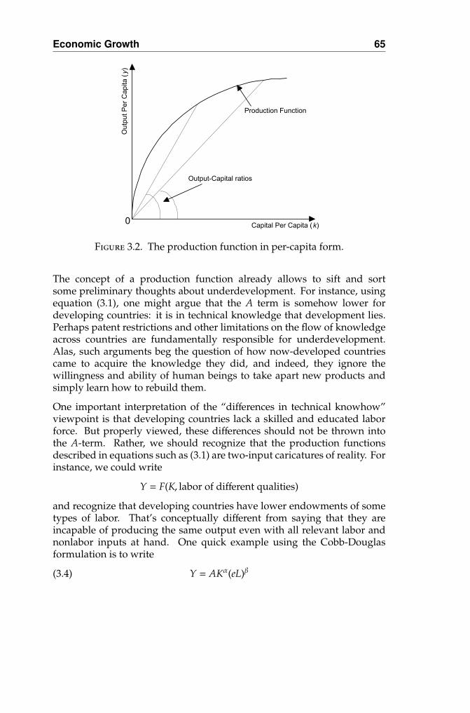
Figure 3.2 depicts a production function in per capita format. Typically,it will display diminishing returns to per-capita capital. As k increases,so does y (of course), but in a progressively more muted way. Thus theoutput-capital ratio y/k will fall as k climbs, because of a relative shortageof labor. Just how quickly it falls will depend on the extent of diminishingreturns to capital.

4One question has to do with whether we can really double all inputs within themathematical frame of the production function. What about, say, that elusive input calledentrepreneurship or oversight: are we doubling that too? If not, output might less thandouble. On the other hand, if bricks-and-mortar build a production facility and we doublethe amount of bricks, the volume of the facility will typically more than double, the formerbeing proportional to surface area and the latter rising at (surface area)3/2.

Economic Growth 65

Figure 3.2. The production function in per-capita form.

The concept of a production function already allows to sift and sortsome preliminary thoughts about underdevelopment. For instance, usingequation (3.1), one might argue that the A term is somehow lower fordeveloping countries: it is in technical knowledge that development lies.Perhaps patent restrictions and other limitations on the flow of knowledgeacross countries are fundamentally responsible for underdevelopment.Alas, such arguments beg the question of how now-developed countriescame to acquire the knowledge they did, and indeed, they ignore thewillingness and ability of human beings to take apart new products andsimply learn how to rebuild them.

One important interpretation of the “di↵erences in technical knowhow”viewpoint is that developing countries lack a skilled and educated laborforce. But properly viewed, these di↵erences should not be thrown intothe A-term. Rather, we should recognize that the production functionsdescribed in equations such as (3.1) are two-input caricatures of reality. Forinstance, we could write

Y = F(K, labor of di↵erent qualities)

and recognize that developing countries have lower endowments of sometypes of labor. That’s conceptually di↵erent from saying that they areincapable of producing the same output even with all relevant labor andnonlabor inputs at hand. One quick example using the Cobb-Douglasformulation is to write

(3.4) Y = AK↵(eL)�

66 Economic Growth

where e is years of schooling per person. That mathematically links upwith “lower A,” but it’s conceptually very di↵erent, pointing the finger asit does to education and not technology.

Another interpretation of “di↵erent A” is that while the same technologiesare available in both developed and developing countries, the resources toeach technology are misallocated in developing countries. For instance,entrepreneurs in the poorer country might not have enough access tocapital or credit markets to raise the funds for the move to a newer andbetter technology. Or the older technology may be in the hands of older,elite groups with political power, who block access to new technologiesthat could spell their own ruin. Or local communities — again, possiblyencouraged by domestic elites — might oppose new technologies for fearthat these will let “foreign interests” into the country.

We will have much to say about these and related issues later in thebook. But our quest for explanations starts with the limited input story.A developing country surely has less capital — physical and human —relative to labor, compared to its developed-country counterpart. Mightthis, and this alone, not explain persistent, ongoing di↵erences in per capitaincome across countries? To understand such matters, we must expand ourtheory to allow capital to be systematically accumulated. That is the job ofthe fundamental “growth equation,” to which we now turn.

3.3.3 The Growth Equation. A little algebra at this stage will make ourlives simpler. Divide time into periods t = 0, 1, 2, 3, . . . .We will tag relevanteconomic variables with the date: Y(t) for output, I(t) for investment, and soon. Investment augments the capital stock after accounting for depreciatedcapital, so in symbols:

K(t + 1) = (1 � �)K(t) + I(t),where � is the rate of depreciation. But we’ve just been going on about thefamous macroeconomic balance condition, that investment equals savings.It follows that I(t) = sY(t), where s is the rate of savings and Y(t) is aggregateoutput, and using this in the equation above, we see that(3.5) K(t + 1) = (1 � �)K(t) + sY(t),which tells us how the capital stock must change over time.

We’re going to convert this into per-capita terms by dividing by the totalpopulation, which we assume (only for expositional simplicity) to be equalto the active labor force L(t). If we assume that population grows at aconstant rate n, so that L(t + 1) = (1 + n)L(t), (3.5) changes to(3.6) (1 + n)k(t + 1) = (1 � �)k(t) + sy(t),

Economic Growth 67

where the lowercase ks and ys represent per capita magnitudes (K/L andY/L, respectively).

This is our basic growth equation: make sure you understand the economicintuition underlying the algebra. It really is very simple. The right-handside has two parts, depreciated per capita capital (which is (1 � �)k(t))and current per capita savings (which is sy(t)). Added together, this shouldgive us the new per capita capital stock k(t+1), except for one complication:population is growing, which exerts a downward drag on per capita capitalstocks. This is why the left-hand side of (3.6) has the rate of growth ofpopulation (n) in it: the larger that rate, the lower is per capita capital stockin the next period.

Take the growth equation for a spin: start in your mind’s eye with the percapita capital stock at any date t, k(t). That produces per capita output y(t)via the production function described in Section 3.3.2. Now the equationtells you what k(t + 1) must be, and the story repeats, presumably withoutend.

3.4 The Solow Model

So far we’ve described the ingredients of a basic growth model, any growthmodel. A more detailed study must rely on a specific form of the productionfunction, and we will start by presuming constant returns to scale anddiminishing returns to each input, as in the Cobb-Douglas formulation ofequation (3.2). The resulting analysis yields a fundamental and much-venerated theory of growth, due to Robert Solow (1957).

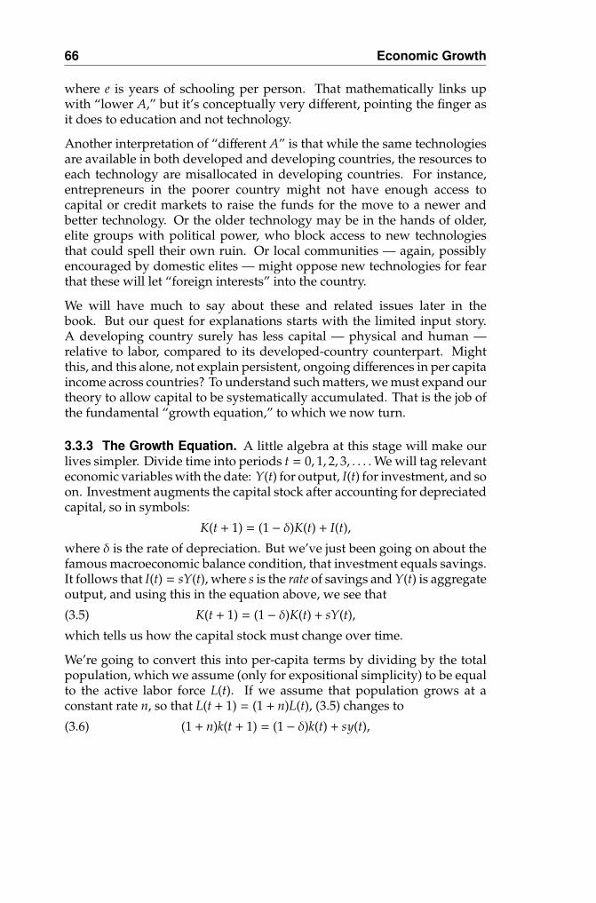
3.4.1 Dynamics of the Growth Equation. Figure 3.3 embeds a produc-tion function with diminishing returns into the growth equation (3.6).Mark any value of k on the horizontal axis, multiply the per capita outputproduced from it by s, which gives us fresh investment, and add the result tothe depreciated value of k. The end product is the curved line in Figure 3.3,which looks very much like the production function itself (and indeed, isclosely related), but has been transformed in the way we’ve just described.Figure 3.3 also plots the left-hand side of (3.6), the straight line (1+ n)k as kchanges. When there are diminishing returns, the curved line initially liesabove this straight line and then falls below.5

5If you’ve been following the argument particularly closely, you will see that this laststatement is exactly true if we make the additional assumption that the marginal product ofcapital is very high when there is very little capital and diminishes to zero as the per capitacapital stock becomes very high.

68 Economic Growth

Figure 3.3. The dynamics of the Solow model.

Armed with this diagram, we can make some very strong predictions aboutgrowth. Figure 3.3 shows us two initial historical levels of the per capitacapital stock — one “low” (Figure 3.3a) and one “high” (Figure 3.3b) —starting, in deference to the year I began writing this book, 1996. Withthe low stock, the marginal return to capital is very high and so the percapita capital stock expands quite rapidly. How do we see this in Figure3.3? Well, we know from (3.6) that the supply of per capita capital is reado↵ by traveling up to the point on the curved line corresponding to theinitial stock k(96). However, some of this supply is eroded by populationgrowth. To find k(97), we simply travel horizontally until the line (1 + n)kis touched; the capital stock corresponding to this point is 1997’s per capitacapital stock. Now just repeat the process. We obtain the zigzag path inFigure 3.3a. Note that the growth of per capita capital slows down and thatper capita capital finally settles close to k⇤, which is a distinguished capitalstock level where the curved and straight lines meet.

Likewise, you may trace the argument for a high initial capital stock, as inFigure 3.3b. Here, there is an erosion of the per capita stock as time passes,with convergence occurring over time to the same per capita stock, k⇤, as inFigure 3.3a. The idea here is exactly the opposite of that in the previousparagraph: the output-capital ratio is low, so the rate of expansion ofaggregate capital is low. Therefore, population growth outstrips the rate ofgrowth of capital, thus eroding the per capita capital stock.

3.4.2 The Steady State. We can think of k⇤ as a steady-state level of theper capita capital stock, to which the per capita capital stock, starting fromany initial level, must converge.

Economic Growth 69

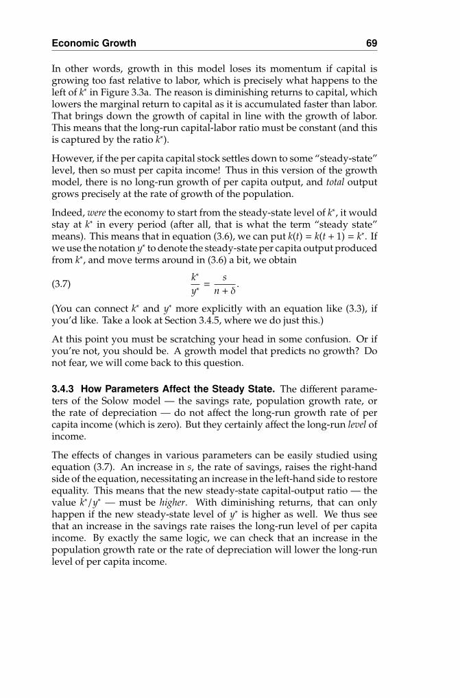
In other words, growth in this model loses its momentum if capital isgrowing too fast relative to labor, which is precisely what happens to theleft of k⇤ in Figure 3.3a. The reason is diminishing returns to capital, whichlowers the marginal return to capital as it is accumulated faster than labor.That brings down the growth of capital in line with the growth of labor.This means that the long-run capital-labor ratio must be constant (and thisis captured by the ratio k⇤).

However, if the per capita capital stock settles down to some “steady-state”level, then so must per capita income! Thus in this version of the growthmodel, there is no long-run growth of per capita output, and total outputgrows precisely at the rate of growth of the population.

Indeed, were the economy to start from the steady-state level of k⇤, it wouldstay at k⇤ in every period (after all, that is what the term “steady state”means). This means that in equation (3.6), we can put k(t) = k(t + 1) = k⇤. Ifwe use the notation y⇤ to denote the steady-state per capita output producedfrom k⇤, and move terms around in (3.6) a bit, we obtain

(3.7)k⇤

y⇤=

sn + �

.

(You can connect k⇤ and y⇤ more explicitly with an equation like (3.3), ifyou’d like. Take a look at Section 3.4.5, where we do just this.)

At this point you must be scratching your head in some confusion. Or ifyou’re not, you should be. A growth model that predicts no growth? Donot fear, we will come back to this question.

3.4.3 How Parameters Affect the Steady State. The di↵erent parame-ters of the Solow model — the savings rate, population growth rate, orthe rate of depreciation — do not a↵ect the long-run growth rate of percapita income (which is zero). But they certainly a↵ect the long-run level ofincome.

The e↵ects of changes in various parameters can be easily studied usingequation (3.7). An increase in s, the rate of savings, raises the right-handside of the equation, necessitating an increase in the left-hand side to restoreequality. This means that the new steady-state capital-output ratio — thevalue k⇤/y⇤ — must be higher. With diminishing returns, that can onlyhappen if the new steady-state level of y⇤ is higher as well. We thus seethat an increase in the savings rate raises the long-run level of per capitaincome. By exactly the same logic, we can check that an increase in thepopulation growth rate or the rate of depreciation will lower the long-runlevel of per capita income.

70 Economic Growth

But as always, make sure you understand the economics behind the algebra.For instance, a higher rate of depreciation means that more of nationalsavings must go into the replacement of worn-out capital. This meansthat, all other things being equal, the economy accumulates a smaller netamount of per capita capital, and this lowers the steady-state level. Youshould similarly run through — verbally — the e↵ects of changes in thesavings rate and the population growth rate.

3.4.4 Technical Progress. We promised to address the no-growth para-dox of the Solow model, and we shall do so at several points, startingnow.

First a quick review of that counterfactual conclusion: given diminishingreturns, the marginal contribution of capital to output must decline whencapital grows faster than population, and increase when capital growsslower than population. That eventually forces the growth rate of aggregatecapital — and output — to equal the growth rate of population, with zerogrowth per capita.

But this is the most parsimonious sca↵olding of the model, which we canmodify in several ways. For instance, the no-growth scenario disappearsif there is continuing technical progress; that is, if the production functionshifts upward over time as new knowledge is gained and applied. As long asthe optimistic force of this shift outweighs the doom of diminishing returns,there is no reason why per capita growth cannot be sustained indefinitely.

This twist on the model makes intuitive sense. Imagine a world in whichwe never learnt to do things better. Then the influence of fixed factors —land, oil, and other resources — would make itself felt, and growth couldconceivably vanish. In our simple model, we are benchmarking everythingrelative to labor by taking per-capita magnitudes, so labor plays the role ofthat fixed factor, and in the absence of technical progress, growth per capitamust slow to a crawl.

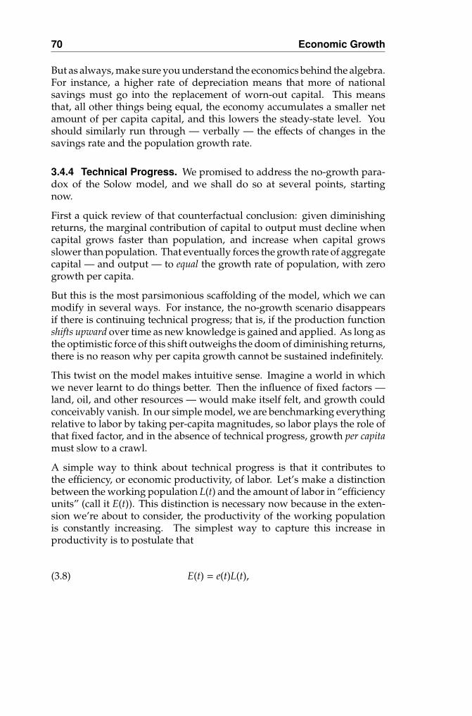
A simple way to think about technical progress is that it contributes tothe e�ciency, or economic productivity, of labor. Let’s make a distinctionbetween the working population L(t) and the amount of labor in “e�ciencyunits” (call it E(t)). This distinction is necessary now because in the exten-sion we’re about to consider, the productivity of the working populationis constantly increasing. The simplest way to capture this increase inproductivity is to postulate that

(3.8) E(t) = e(t)L(t),

Economic Growth 71

0 k^k*^

(1+n )(1+ �) k^

(1- � ) k�+�sy^ ^

Capital per efficiency unit

Out

put p

er e

fficie

ncy

unit

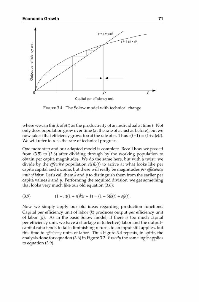
Figure 3.4. The Solow model with technical change.

where we can think of e(t) as the productivity of an individual at time t. Notonly does population grow over time (at the rate of n, just as before), but wenow take it that e�ciency grows too at the rate of⇡. Thus e(t+1) = (1+⇡)e(t).We will refer to ⇡ as the rate of technical progress.

One more step and our adapted model is complete. Recall how we passedfrom (3.5) to (3.6) after dividing through by the working population toobtain per capita magnitudes. We do the same here, but with a twist: wedivide by the e↵ective population e(t)L(t) to arrive at what looks like percapita capital and income, but these will really be magnitudes per e�ciencyunit of labor. Let’s call them k and y to distinguish them from the earlier percapita values k and y. Performing the required division, we get somethingthat looks very much like our old equation (3.6):

(3.9) (1 + n)(1 + ⇡)k(t + 1) = (1 � �)k(t) + sy(t).

Now we simply apply our old ideas regarding production functions.Capital per e�ciency unit of labor (k) produces output per e�ciency unitof labor (y). As in the basic Solow model, if there is too much capitalper e�ciency unit, we have a shortage of (e↵ective) labor and the output–capital ratio tends to fall: diminishing returns to an input still applies, butthis time to e�ciency units of labor. Thus Figure 3.4 repeats, in spirit, theanalysis done for equation (3.6) in Figure 3.3. Exactly the same logic appliesto equation (3.9).

72 Economic Growth

Over time, the amount of capital per e↵ective labor may rise or fall. Observethat if it is rising, this simply means that physical capital is growingfaster than the rate of population growth and technical progress combined.However, by diminishing returns, output per e�ciency unit rises less thanproportionately. That tones down the subsequent growth rate of capitalper e�ciency unit. In Figure 3.4, this discussion corresponds to the regionlying left of the intersection point k⇤. In this region, the growth rate of totalcapital falls over time as capital per e�ciency unit rises. Likewise, to theright of the intersection, capital per e�ciency unit falls over time. Onceagain, we have convergence, this time to the steady-state level k⇤.

To solve for the steady state, put k(t) = k(t + 1) = k⇤ in (3.9), just as we didto arrive at the steady state formula without technical progress; see (3.7).That gives us

(1 + n)(1 + ⇡)k⇤ = (1 � �)k⇤ + sy⇤,and rearranging this equation, we conclude that

k⇤

y⇤=

s(1 + n)(1 + ⇡) � (1 � �) .

For an easy-to-remember version of this equation, note that both⇡ and n aresmall numbers, such as 0.05 or 0.02, so their product is very small relativeto the other terms and can be ignored in a first-order approximation. Somultiplying out (1 + n)(1 + ⇡) and ignoring the term n⇡, we see that

(3.10)k⇤

y⇤' s

n + ⇡ + �.

(Once again, just as for equation (3.7), you can connect k⇤ and y⇤ with aspecific production function, as we will do in Chapter 4, Section 4.3.4.)

So far the analysis runs parallel to the case of no technical progress. Thenovelty lies in the interpretation. Even though capital per e�ciency unitconverges to a stationary steady state, the amount of capital per memberof the working population continues to increase. Indeed, the long-runincrease in per capita income takes place precisely at the rate of technicalprogress.

In summary, think of two broad sources of growth: one is through betterand more advanced methods of production (technical progress) and thesecond is via the continued buildup of plant, machinery, and other inputsthat bring increased productive power.6 The Solow model claims that in

6This is not to deny that these two sources are often intimately linked: technical progressmay be embodied in the new accumulation of capital inputs.

Economic Growth 73

the absence of the first source, the second is not enough for sustained per capitagrowth. Viewed in this way, the Solow model is a pointer to studying theeconomics of technological progress, arguing that it is there that one mustlook for the ultimate sources of growth. This is not to say that such a claimis necessarily true, but it is certainly provocative and very far from beingobviously wrong.

3.4.5 Another Route to Sustained Growth: The Harrod-Domar Model.Let’s take a second look at sustained growth. Eliminate technical progressfor the moment, and return to the fundamental growth equation (3.6),reproduced here for easy reference:(3.11) (1 + n)k(t + 1) = (1 � �)k(t) + sy(t).This turns into the Solow model under the additional assumption ofdiminishing returns to capital. That assumption creates variation in thecapital-output ratio, allowing the economy to settle at the distinguishedlevel k⇤ given by

(3.12)k⇤

y⇤=

sn + �

,

which is equation (3.7), again reproduced here. (This second equation isobtained, as already discussed, by setting k(t) = k(t+1) = k⇤ and y(t) = y⇤ inthe growth equation (3.11), and solving out for corresponding ratio k⇤/y⇤.)A solution exists because k/y varies from very high to very low values overthe range of the production function.7 For instance, when the productionfunction is Cobb-Douglas, so that

y = Ak↵,

the steady state condition (3.12) becomesk⇤

Ak⇤↵=

sn + �

,

so that after a little not-so-tedious algebra, we see that

(3.13) k⇤ =✓ sAn + �

◆1/(1�↵).

This is a simple and rewarding equation, because you can “see” the steadystate as explicitly as possible, and what is more, you can redo all theparametric exercises of Section 3.4.3 in a flash simply by eyeballing (3.13).

But there is something else that I’d like to draw your attention to. Lookat the “diminishing returns parameter” ↵ and remember that the smaller

7The careful reader will observe again that we’re assuming diminishing returns plus suitableend-point conditions on the marginal product of capital.

74 Economic Growth

it is, the more it is that returns diminish, while at the other end, as ↵becomes close to 1, the production function becomes almost linear andexhibits constant returns to capital. As we bring ↵ up close to 1, the steadystate level of capital becomes ever larger (if sA > n + �) or ever smaller (ifsA < n+�) and at ↵ equal to 1, when the production function is exactly linearin capital, there is no steady state: the economy either grows to infinity orshrinks to zero! This is not an algebraic sleight of hand; on the contrary,it makes intuitive sense. The easiest way to see it is to appreciate thatwhen ↵ = 1, the current scale of the economy (proxied by k) is irrelevant:whatever rate it can grow at k, it can replicate that at 2k, 3k, or a milliontimes k. With diminishing returns, that isn’t possible, which is why a steadystate is ultimately reached, but when there is constant returns to the capitalinput, everything can grow or decline at exactly the same rate, irrespectiveof scale.

The fundamental growth equation (3.11) can handle this without a problem,provided we don’t go down the garden path looking for steady states wherethere are none to be found. With constant returns to scale, the output-capitalratio is a constant; in fact, it is exactly A in the Cobb-Douglas productionfunction with ↵ = 1: y = Ak. Using this in the growth equation yields

(1 + n)k(t + 1) = (1 � �)k(t) + sAk(t),

and after the inevitable moving-around of terms, we have

(3.14) Rate of growth =k(t + 1) � k(t)

k(t)=

sA � (n + �)1 + n

.

This is an influential relationship, known as the Harrod-Domar equation.named after Roy Harrod and Evsey Domar, who wrote some of the earliestpapers on the subject in 1939 and 1946, respectively. The left-hand side isjust the rate of growth of the per capita capital stock, and by the linearityof the production function it is also the rate of growth of per capita income.Time appears here on the left-hand side, but it doesn’t in the rest of theequation, which shows that the rate of growth is constant and unchanging.What is more, it provides a formula for that rate of growth, given by theright-hand side of (3.14).

For an easy-to-remember version of (3.14), let g stand for the rate ofgrowth, multiply through by 1 + n, and note that both g and n are smallnumbers (analogous to our approach to deriving (3.10)), and their productgn is therefore extra small relative to these numbers. That gives us theapproximation

(3.15) sA ' g + n + �,

Economic Growth 75

which can be used in place of (3.14) without much loss of accuracy.

It isn’t hard to see why this equation was influential. It has the air of arecipe. Thomas Piketty, in his book Capital (2014) — on which more later— calls it the “second fundamental law of capitalism.” The equation firmlylinks the growth rate of the economy to fundamental variables, such asthe ability of the economy to save, the capital–output ratio and the growthrate of population. And capitalism apart, central planning in countriessuch as India and the erstwhile Soviet Union was deeply influenced by theHarrod–Domar equation (see box).

Growth Engineering: The Soviet Experience

The Harrod–Domar model, as we have seen, has both descriptive and prescriptivevalue. The growth rate depends on certain parameters and, in a free marketeconomy, these parameters are determined by people’s tastes and technology.However, in a socialist, centrally planned economy (or even in a mixed economywith a large public sector), the government may have enough instruments (suchas direct control over production and allocation, strong powers of taxation andconfiscation, etc.) to manipulate these parameters to influence the growth rate.Given a government’s growth objectives and existing technological conditions(e.g., the capital–output ratio), the Harrod–Domar model can be used to obtainpolicy clues; for example, the desired rate of investment to be undertaken so as toachieve this aim.

The first controlled experiment in “growth engineering” undertaken in the worldwas in the former Soviet Union, after the Bolshevik Revolution in 1917. Theyears immediately following the Revolution were spent in a bitter struggle—between the Bolsheviks and their various enemies, particularly the White Armyof the previous Czarist regime—over the control of territory and productive assetssuch as land, factories, and machinery. Through the decade of the 1920s, theBolsheviks gradually extended control over most of the Soviet Union (consistingof Russia, Ukraine, and other smaller states) that encompassed almost the whole ofindustry, channels of trade and commerce, food-grain distribution, and currency.The time had come, therefore, to use this newly acquired control over the economicmachinery to achieve the economic goals of the revolutionary Bolsheviks, theforemost among these goals being a fast pace of industrialization.8

8On the eve of the Revolution, Russia took a back seat among European nations in extentof industrialization, despite a rich endowment of natural resources. According to thecalculations of P. Bairoch, based on the per capita consumption of essential industrial inputs,namely, raw cotton, pig iron, railway services, coal, and steam power, Russia ranked lastamong nine major European nations in 1910, behind even Spain and Italy. See Nove [1969].

76 Economic Growth

1927–28 (actual) 1932–33 (plan) 1932 (actual)

National income 24.4 49.7 45.5Gross industrial production 18.3 43.2 43.3

(a) Producers’ goods 6.0 18.1 23.1(b) Consumers’ goods 12.3 25.1 20.2

Gross agricultural production 13.1 25.8 16.6Source: Dobb [1966].

aAll figures are in 100 million 1926–27 rubles.Table 3.3. Targets and achievements of the first Soviet fiveYear Plan (1928–29 to 1932–33).a

Toward the end of the 1920s, the need for a coordinated approach to tackle theproblem of industrialization on all fronts was strongly felt. Under the auspicesof the State Economic Planning Commission (called the Gosplan), a series ofdraft plans was drawn up which culminated in the first Soviet Five Year Plan(a predecessor to many more), which covered the period from 1929 to 1933. At thelevel of objectives, the plan placed a strong emphasis on industrial growth. Theresulting need to step up the rate of investment was reflected in the plan targetof increasing it from the existing level of 19.9% of national income in 1927–28 to33.6% by 1932–33. (Dobb [1966, p. 236]).

How did the Soviet economy perform under the first Five Year Plan? Table 3.3shows some of the plan targets and actual achievements, and what emerges is quiteimpressive. Within a space of five years, real national income nearly doubled,although it stayed slightly below the plan target. Progress on the industrial frontwas truly spectacular: gross industrial production increased almost 2.5 times.This was mainly due to rapid expansion in the machine producing sector (wherethe increment was a factor of nearly 4, far in excess of even plan targets), whichis understandable, given the enormous emphasis on heavy industry in order toexpand Russia’s meager industrial base. Note that the production of consumergoods fell way below plan targets.

An equally spectacular failure shows up in the agricultural sector, in which actualproduction in 1932 was barely two-thirds of the plan target and only slightly morethan the 1927–28 level. The reason was probably that the Bolsheviks’ control overagriculture was never as complete as that over industry: continuing strife withthe kulak farmers (large landowners from the Czarist era) took its toll on cropproduction.

Unlike the Solow model, the Harrod-Domar variant it generates sustainedgrowth without having to invoke technical progress. And yet, does that make

Economic Growth 77

it a “better” model? Not necessarily. There is a price to be paid for theresult, which is that the model assumes that labor is not a serious constrainton production at all (if it were, the returns to ever more capital, holdinglabor constant, would presumably diminish). But matters are a bit morecomplicated than that. In real life, there aren’t just two inputs, “capital”and “labor.” There is a whole host of them, and the predictive power ofHarrod-Domar versus Solow would ultimately stand or fall on the combineddiminishing returns — or lack thereof — of all those inputs relative to rawlabor.

We will be back to Solow versus Harrod-Domar at a later stage. For now,my only request is that you don’t get confused. It doesn’t matter that onemodel generates sustained growth while the other doesn’t. They rely, asI’ve tried to make clear, on di↵erent assumptions. Therefore, which modelis more relevant is ultimately an empirical question and, as we shall soonsee, the jury is still out on the issue. For now, the takeaway point is thatconstant technical progress is needed to generate sustained growth in theface of diminishing returns to capital, while capital accumulation per se isenough to do the trick when the return to capital is constant (or increasing).