Economic Growth and Financial Depth - UNU-WIDER€¦ · · 2015-08-18advocacy of policies leading ... country and panel datasets for the post-1960 period.2 The influence of financial

Copyright © UNU-WIDER 2005 1Vanderbilt University, [email protected]; 2Stern School of Business, [email protected]

This study has been prepared within the UNU-WIDER project on Financial Sector Development for Growth and Poverty Reduction, directed by Basudeb Guha-Khasnobis and George Mavrotas.

UNU-WIDER acknowledges the financial contributions to the research programme by the governments of Denmark (Royal Ministry of Foreign Affairs), Finland (Ministry for Foreign Affairs), Norway (Royal Ministry of Foreign Affairs), Sweden (Swedish International Development Cooperation Agency–Sida) and the United Kingdom (Department for International Development).

Discussion Paper No. 2005/10 Economic Growth and Financial Depth Is the Relationship Extinct Already? Peter L. Rousseau1 and Paul Wachtel2 December 2005

Abstract

Although the finance–growth nexus has become firmly entrenched in the empirical literature, studies that question the strength of the empirical results have appeared and seem to have become more frequent as well. In this paper we re-examine the core cross-country panel results that established the relationship between financial depth and growth rates. We examine the sensitivity of the core result to changes in time period and variation in the sample of countries included. We find that the finance–growth relationship in not as strong with more recent data as it was in the original studies with data for the period from 1960 to 1989. We offer two possible explanations. First, financial depth may have had greater value as a shock absorber in the 1970s and 1980s, decades characterized by worldwide nominal shocks Second, the spread of financial liberalization in the 1980s may have led to increasing financial depth in countries that lacked the legal or regulatory infrastructure to successfully exploit financial development. …/ Keywords: finance–growth nexus, rolling regression, robustness, cross-country growth JEL classification: E44, G10, O40

The World Institute for Development Economics Research (WIDER) was established by the United Nations University (UNU) as its first research and training centre and started work in Helsinki, Finland in 1985. The Institute undertakes applied research and policy analysis on structural changes affecting the developing and transitional economies, provides a forum for the advocacy of policies leading to robust, equitable and environmentally sustainable growth, and promotes capacity strengthening and training in the field of economic and social policy making. Work is carried out by staff researchers and visiting scholars in Helsinki and through networks of collaborating scholars and institutions around the world. www.wider.unu.edu [email protected]

UNU World Institute for Development Economics Research (UNU-WIDER) Katajanokanlaituri 6 B, 00160 Helsinki, Finland Camera-ready typescript prepared by Lorraine Telfer-Taivainen at UNU-WIDER Printed at UNU-WIDER, Helsinki The views expressed in this publication are those of the author(s). Publication does not imply endorsement by the Institute or the United Nations University, nor by the programme/project sponsors, of any of the views expressed. ISSN 1609-5774 ISBN 92-9190-748-0 (printed publication) ISBN 92-9190-749-9 (internet publication)

We use a rolling regression technique to see which countries provide stronger support for the finance growth relationship. Among poorer counties the relationship is positive but imprecisely measured, and among very rich countries it is absent. However, there is clear indication that financial deepening increases growth among the countries with real GDP per capita betweenUS$3,000 andUS$12,000 (1995). In sum, we find the widely accepted effect of finance on growth to be still present but fragile.

Acknowledgements

This paper was prepared for the UNU-WIDER conference on Financial Sector Development for Growth and Poverty Reduction, 1-2 July 2005, Helsinki.

1

1 Introduction

Among the profound changes to development economics in recent years has been the renewed emphasis on the role of the financial sector in promoting economic growth. Historical antecedents to the current revival of interest in the topic include, among others, Goldsmith (1969)1 and McKinnon (1973), who drew attention to the contributions of financial structure to growth and the benefits of financial liberalization. Since then, economists have slowly acknowledged that the tools of early development economists—credit allocation, interest rate ceilings and high reserve requirements—were undesirable. In 1991 (p.12) McKinnon could write with confidence that, ‘Now, however, there is widespread agreement that flows of saving and investment should be voluntary and significantly decentralized in an open capital market at close to equilibrium interest rates’. Indeed, the prevailing contemporary paradigm is that competitive private sector capital markets should be able to gather savings at market rates of interest and allocate capital to the most efficient private sector projects. What is most puzzling is that the contemporary paradigm emerged well before there was any solid evidence that related the financial sector to economic growth and stability. Thus, the initial efforts to demonstrate the positive relationship empirically were truly important contributions. The seminal work is King and Levine (1993), which extended the cross-country framework introduced in Barro (1991) by adding financial variables such as the ratios of liquid liabilities or claims on the private sector to gross domestic product (GDP) to the standard growth regression. They found a robust, positive, and statistically significant relationship between initial financial conditions and subsequent growth in real per capita incomes. Over the past decade, a number of empirical studies have expanded upon this, using both cross-country and panel datasets for the post-1960 period.2 The influence of financial development on economic growth shown in this literature is now a firmly established part of the economics cannon. The large literature that uses cross-country and panel data to investigate the sources of long-run economic growth also explores the sensitivity of the standard regression to the inclusion of conditioning variables such as government expenditure, the extent of international trade, and inflation. Levine and Renelt (1992), for example, used a wide range of policy and economic indicators to demonstrate the fragility of many cross-country links between growth on one

1 Goldsmith (1969), for example, found a positive relationship between economic growth and financial development using a comparative approach with data for thirty-five countries over the period 1860-1963. 2 Levine (1997) offers an excellent survey of the literature through the mid 1990s. Levine (2005) is a comprehensive treatment of the many contributions that have followed. See also Temple (1999).

2

hand and political and institutional factors on the other.3 Interestingly, the Levine and Renelt article predates the renewed interest in the finance–growth relationship and did not consider the robustness of financial factors in the standard growth regression. Although the finance–growth nexus has become firmly entrenched, studies that question the strength of the empirical results have appeared and seem to have become more frequent as well. Economists as disparate as Joan Robinson and Robert Lucas have expressed doubts about the link.4 More importantly, a number of authors have been less than enthusiastic about the strength of the recently established empirical consensus. While American authors (e.g., Levine and ourselves) often exhibit unbounded enthusiasm about the strength of the relationship, Europeans (Arestis, Demetriades and Temple, among others) are much more cautious and give more emphasis to the variability of the effects and the lack of robustness in some studies. Moreover, in the last few years a number of papers have appeared whose titles express the growing skepticism.5 Among the empirical studies that take issue with the cross-country findings is Demetriades and Hussein (1996), which uses time-series for sixteen less developed countries and finds that causality between finance and growth varies considerably across them. Arestis et al. (2001) show that the relationship exhibits considerable variation even among developed countries. Rousseau and Wachtel (1998) and Rioja and Valev (2004) suggest that the relationship varies with the level of economic development. Arestis and Demetriades (1997) and Wachtel (2003) consider potential conceptual and methodological problems associated with inferring causation from cross-country correlations. Our intention in this paper is to re-examine the core panel result. Earlier work has exposed it to careful econometric analysis and the result stands up to a barrage of sophisticated techniques—instrumental variables, panel dynamics, etc. However, the robustness of the result over time, especially in the past fifteen years, provides reason for pause and the sensitivity of the relationship to some particular small perturbations to the specification is troubling. Small changes in the sample of countries included in the regressions also have considerable effects. Here we address these issues and attempt to document how robust the standard finding happens to be.

3 Levine and Renelt (1992) found partial correlations to be robust only between growth and the investment rate and between the investment rate and the ratio of international trade to GDP. 4 Lucas (1988) suggests that the role of finance is ‘over-stressed’ and Robinson (1952: 80) asserts that ‘where enterprise leads, finance follows’. 5 For example, ‘How Much Do We Really Know about Growth And Finance?’ Wachtel (2003); and ‘Finance Causes Growth: Can We Be So Sure?’ Manning (2003), among others.

3

The next section describes the data and the by now standard approach to panel estimates of growth equations. In the following section we present baseline estimates and begin our investigation of robustness. The first issue is whether the finance relationship is as strong with more recent data as it appears in the original studies with data for the period from 1960 to 1989. The second issue addressed is whether the panel data results depend on unobserved or unmodeled country characteristics that are just well proxied by the finance measures. The fourth section explores the influence of country effects and the choice of countries included in the sample. In a word, we find the widely accepted effect of finance on growth to be fragile. We elaborate in the conclusion and consider possible explanations.

2 Data and methodology

Our study includes cross sectional and panel data on financial and macroeconomic indicators for 84 countries over the period 1960-2003.6 Data are from the 2004 version of the World Bank’s World Development Indicators database. To ensure comparability with King and Levine’s original study and others, we use three familiar measures of financial development, namely the ratios to GDP of liquid liabilities (M3), liquid liabilities less narrow money (M3 less M1), and credit allocated to the private sector. M3 as a percent of GDP has become a standard measure of financial depth and an indicator of the overall size of financial intermediary activity in cross-country studies. M3 less M1 removes the pure transactions asset and the credit measure isolates intermediation to the private sector from credit allocated to government or state enterprises.7 King and Levine’s (1993) version of the Barro growth regression, and the starting point for our analysis, has the form

Yit = α0 + αFit + βX it + uit, (1)

6 Our panel of 84 countries includes all for which the requisite WDI data are available. They are Algeria, Argentina, Australia, Austria, Bangladesh, Barbados, Belgium, Bolivia, Brazil, Cameroon, Canada, Central African Republic, Chile, Colombia, Costa Rica, Cote d’Ivoire, Denmark, Dominican Republic, Ecuador, Egypt, El Salvador, Fiji, Finland, France, Gambia, Ghana, Greece, Guatemala, Guyana, Haiti, Honduras, Iceland, India, Indonesia, Iran, Ireland, Israel, Italy, Jamaica, Japan, Jordan, Kenya, Republic of Korea, Lesotho, Luxembourg, Malawi, Malaysia, Malta, Mauritius, Mexico, Morocco, Nepal, Netherlands, New Zealand, Nicaragua, Niger, Nigeria, Norway, Pakistan, Panama, Papua New Guinea, Paraguay, Peru, Philippines, Portugal, Rwanda, Senegal, Sierra Leone, South Africa, Spain, Sri Lanka, Sudan, Sweden, Switzerland, Syrian Arab Republic, Thailand, Trinidad and Tobago, Togo, Turkey, United Kingdom, United States, Uruguay, Venezuela, and Zimbabwe. 7 Studies such as Levine and Zervos (1998) and Rousseau and Wachtel (2000) expand the set of financial indicators to include measures of stock market size, trading, and turnover. Most find a significant positive correlation between these measures of market activity and growth. Using these measures would limit the scope of our study to those countries and years for which stock market data are available, reducing the number of observations by nearly half. Since our aim is to examine the robustness of the most fundamental links between

4

where Yit is the growth rate of real per capita GDP, Fit is a measure of financial sector development, and Xit is a set of baseline explanatory variables that have been shown empirically to be robust determinants of growth. The X variables include the log of initial real per capita GDP, which should capture the tendency for growth rates to converge across countries and over time, and the log of the initial secondary school enrollment rate, which should reflect the extent of investment in human capital. We also consider specifications that include the ratio of trade (i.e., imports plus exports) to GDP and the ratio of government final consumption to GDP as supplemental elements of X. We estimate equation (1) with a panel of 5-year averages from 1960 to 2003.8 To reduce any simultaneity bias that would result from the influence of economic growth on the development of the financial sector, we follow the literature and use instrumental variables (two-stage least squares). Specifically, we attempt to extract the predetermined component of F by using its initial value (in the 5-year average) along with the initial values of government expenditure and trade as percentages of GDP as instruments in each regression equation.

3 Baseline regression estimates and robustness across time periods

Table 1 contains results from the baseline growth equations. For each of the three measures of financial depth, we show two regression specifications. The first includes only the log of initial real GDP (in constant 1995 US$) and log of the secondary school enrollment rate while the second adds government expenditure and trade, both as percentages of GDP. These baseline results are by and large consistent with the consensus in the literature. The coefficients on the financial variables are positive and usually significant. However, the coefficients are smaller than those in King and Levine (1993) and the coefficient on the credit ratio is not statistically significant in one of the specifications and is significant at only the 10 percent level in the other. This suggests that there might be some heterogeneity in the sample over time that needs to be explored. The coefficients on the financial ratios are relatively unaffected when the two additional regressors—government expenditure and trade as percentages of GDP—are included in the specifications. There are some differences in other coefficients between the two specifications. Only in the simpler specification is the coefficient on the log of initial real GDP negative (although not statistically significant), which supports the notion of beta convergence. The positive and significant coefficient on the log of the secondary school enrollment rate suggests that human capital investment matters for growth.

finance and long-run growth found in the early literature on the subject, we prefer a compact yet thorough treatment of the more traditional measures of financial sector development. 8 There is thus a maximum of nine panel observations for each country. The last panel observation includes data averaged over only four years.

5

Table 1: Baseline instrumental variables growth regressions, 1960-2003

Dependent variable: % Growth of per capita real GDP

(1) (2) (3) (4) (5) (6)

Log of initial real per capita GDP (1995 US$)

-0.143 (0.102)

0.005 (0.107)

-0.168 (0.104)

-0.034 (0.109)

-0.082 (0.116)

0.024 (0.118)

Log of secondary school enrollment rate

0.750** (0.178)

0.681** (0.177)

0.757** (0.178)

0.705** (0.177)

0.878** (0.176)

0.812** (0.174)

Liquid liabilities (M3) (% of GDP)

0.017** (0.004)

0.017** (0.004)

M3 less M1 (% of GDP)

0.026** (0.005)

0.023** (0.006)

Private sector credit (% of GDP)

0.006 (0.004)

0.007* (0.004)

Government expenditure (% of GDP)

-0.084** (0.022)

-0.083** (0.023)

-0.077** (0.021)

Trade (% of GDP)

0.009** (0.004)

0.009** (0.004)

0.012** (0.003)

R2 (no. observations)

.218 (625)

.251 (620)

.235 (605)

.262 (601)

.202 (639)

.241 (633)

Note: The table reports coefficients from two-stage least squares regressions using 5-year averages of the data with standard errors in parentheses. Instruments include initial values of government expenditure, international trade, and the respective financial variable as a percentage of GDP, with initial values taken as the first observation of each 5-year period. The regressions also include dummy variables for the 5-year time periods. * and ** denote statistical significance at the 10 percent and 5 percent levels respectively.

Source: Authors’ calculations.

The differences in these results from earlier published work with the same data definitions call for explanation. Our results extend the datasets used in earlier work to 2003 while the data in King and Levine’s groundbreaking paper ends in 1989.9 In Table 2 we present estimates of the two baseline equations for two time periods. The first period, 1960-89, coincides with the data used by King and Levine (1993) and others that established the consensus results that have

9 In addition, later editions of the World Bank’s World Development Indicators provide some estimates for observations in earlier years that were previously missing. On the other hand, there are fewer observations in the last panel because once the euro was established financial depth ratios were no longer calculated for the countries in the euro area.

Table 2: Instrumental variables growth regressions for two subperiods

Dependent variable: % growth of per capita real GDP

1960-1989 1990-2003

Log of initial real per

capita GDP (1995 US$)

-0.054

(0.123)

-0.037

(0.126)

-0.137

(0.132)

-0.064

(0.134)

-0.118

(0.146)

-0.056

(0.146)

-0.402**

(0.194)

-0.101

(.217)

-0.373**

(0.188)

-0.101

(.211)

-0.261**

(0.207)

-0.077

(.217)

Log of secondary school

enrollment rate

0.528**

(0.196)

0.508**

(0.193)

0.616**

(0.196)

0.601**

(0.104)

0.716**

(0.194)

0.676**

(0.191)

1.505**

(0.454)

1.236**

(0.458)

1.444**

(0.463)

1.238**

(0.465)

1.504**

(0.432)

1.320**

(0.430)

Liquid liabilities (M3)

(% of GDP)

0.026**

(0.006)

0.028**

(0.006)

0.008

(0.006)

0.003

(0.007)

M3 less M1

(% of GDP)

0.033**

(0.007)

0.034**

(0.007)

0.014*

(0.008)

0.007

(0.009)

Private sector credit

(% of GDP)

0.021**

(0.007)

0.024**

(0.007)

0.001

(0.005)

-0.007

(0.006)

Government expenditure

(% of GDP)

-0.086**

(0.028)

-0.074**

(0.029)

-0.075**

(0.027)

-0.084**

(0.038)

-0.100**

(0.041)

-0.080**

(0.036)

Trade (% of GDP)

0.005

(0.005)

0.006

(0.005)

0.012**

(0.005)

0.015**

(0.005)

0.014**

(0.005)

0.013**

(0.004)

R2

(no. observations)

.272

(412)

.298

(412)

.272

(410)

.292

(410)

.257

(412)

.289

(412)

.096

(213)

.148

(208)

.121

(195)

.168

(191)

.099

(227)

.158

(221)

Note: The table reports coefficients from two-stage least squares regressions with standard errors in parentheses. Instruments include initial values of government expenditure, international trade, and the respective financial variable, with initial values taken as the first observation of each 5-year period. The regressions also include dummy variables for the 5-year time periods. * and ** denote statistical significance at the 10 percent and 5 percent levels respectively.


6

7

become so important. The second period, which runs from 1989 to 2003, is shorter but each panel equation still includes about 200 observations. The differences between the two time periods are dramatic. The effect of financial depth on growth, which is always significant in the first 30-year period, all but disappears in the next 15. Whereas all of the F coefficients are significant at the 5 percent level in the early time period, only one is significant at the 10 percent level in the more recent data. The coefficients on the M3 ratio fall by two-thirds and the others by more. Interestingly, the standard errors of the estimates are about the same in both periods. That is, the precision of the estimates is unchanged; the effects are simply smaller and therefore not significantly different from zero. The other coefficients in the growth equations are relatively stable across time periods.

Table 3: Instrumental variables growth regressions with M3 (% of GDP), 5-year cross sections, 1960-2003


1960-64 1965-69 1970-74 1975-79 1980-84 1985-89 1990-94 1995-99 2000-03

Constant

-0.608

(2.291)

1.230

(1.53)

1.608

(1.672)

2.180

(1.782)

-2.236

(1.670)

-2.685*

(1.592)

-5.030**

(1.934)

-1.774

(1.464)

3.139

(3.004)



0.470

(0.360)

-0.285

(0.262)

-0.085

(0.303)

-0.016

(0.359)

-0.131

(0.336)

0.330

(0.286)

-0.028

(0.395)

-0.024

(.282)

-0.253

(.465)


enrollment rate

0.348

(0.448)

0.783**

(0.330)

0.629

(0.433)

-0.162

(0.562)

0.720

(0.610)

0.684

(0.603)

1.911**

(0.797)

0.950

(0.621)

-0.313

(1.046)

Liquid liabilities (M3)

(% of GDP)

-0.003

(0.019)

0.044**

(0.013)

0.033**

(0.013)

0.040**

(0.016)

0.035**

(0.015)

0.015

(0.012)

-0.001

(0.014)

-0.001

(0.009)

0.016

(0.014)

Government expenditure

(% of GDP)

-0.033

(0.113)

0.014

(0.066)

-0.085

(0.067)

-0.128*

(0.072)

-0.022

(0.062)

-0.186**

(0.059)

-0.177**

(0.072)

-0.019

(0.051)

-0.037

(0.073)

Trade (% of GDP) -0.006

(0.014)

-0.006

(0.011)

0.003

(0.012)

0.019

(0.013)

-0.007

(0.012)

0.020*

(0.010)

0.025**

(0.010)

0.005

(0.007)

0.012

(0.011)

R2

(no. observations)

.133

(52)

.371

(66)

.218

(67)

.101

(74)

.115

(78)

.249

(75)

.268

(81)

.098

(79)

.103

(48)

Note: The table reports coefficients from two-stage least squares regressions with standard errors in parentheses. Instruments include initial values of the full set of regressors, with initial values taken as the first observation of each 5-year period. * and ** denote statistical significance at the 10 percent and 5 percent levels respectively.


To further examine the differences over time in the effect of financial depth on growth we estimated the baseline equation separately with the cross section of data from each 5-year period. That is, from 1960 to 2003 there are nine cross sections. Estimates from instrumental variable regressions with each of the three measures of financial depth are shown in Tables 3 to 5 for the M3, M3 less M1 and private credit ratios respectively.10

10 The tables show the specification that includes the government expenditure and trade variables. The results without these variables are indistinguishable.

8

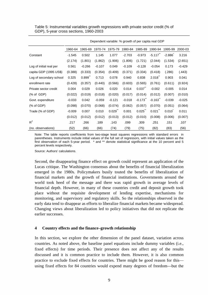
The coefficient on M3 as a percent of GDP is positive and significant for four successive time periods running from 1965 to 1984 but insignificant in the earlier and subsequent periods (Table 3). The same is true for the coefficients on M3 less M1 (Table 4) with the exception of one time period in the 1970s where the coefficient drops. In contrast, the coefficient on the private credit ratio is only significantly different from zero in one time period (Table 5). But the coefficient on private sector credit is clearly positive (averaging .025) from the late 1960s to the early 1990s and then falls to zero or below. The coefficient on the M3 ratio falls to zero from 1985 on and the coefficient on M3 less M1 falls to zero from 1990 on.

Table 4: Instrumental variables growth regressions with M3 less M1 (% of GDP), 5-year cross sections, 1960-2003


1960-64 1965-69 1970-74 1975-79 1980-84 1985-89 1990-94 1995-99 2000-03

Constant

-1.487

(2.455)

1.675

(1.539)

3.197

(1.996)

1.070

(1.958)

-1.526

(1.829)

-1.444

(1.620)

-4.264**

(2.092)

-2.319

(1.722)

2.251

(2.033)



0.464

(0.392)

-0.350

(0.256)

-0.265

(0.342)

0.136

(0.382)

-0.247

(0.355)

0.083

(0.284)

-0.130

(0.408)

0.062

(.306)

-0.292

(.376)

Log of secondary

school enrollment rate

0.514

(0.482)

0.725**

(0.318)

0.528

(0.456)

0.056

(0.580)

0.819

(0.606)

0.718

(0.564)

1.833**

(0.821)

0.956

(0.711)

0.217

(0.837)

M3 less M1

(% of GDP)

0.003

(0.026)

0.066**

(0.014)

0.044**

(0.020)

0.012

(0.019

0.039**

(0.018)

0.035**

(0.013)

0.012

(0.014)

-0.007

(0.015)

0.001

(0.016)

Govt. expenditure

(% of GDP)

-0.031

(0.123)

0.068

(0.065)

-0.060

(0.069)

0.129*

(0.078)

-0.011

(0.065)

-0.172**

(0.057)

-0.174**

(0.077)

-0.035

(0.057)

-0.033

(0.069)

Trade (% of GDP)

-0.002

(0.015)

-0.011

(0.011)

0.006

(0.012)

0.027**

(0.013)

-0.006

(0.013)

0.015

(0.010)

0.023**

(0.010)

0.009

(0.008)

0.013

(0.009)

R2

(no. observations)

.181

(55)

.441

(64)

.158

(68)

.134

(73)

.119

(77)

.297

(73)

.279

(76)

.109

(72)

.099

(43)



These tables provide a clear story. The finance effect on growth is a disappearing phenomenon. We will tender two possible explanations for this striking result. First, there may be something about the 1970s and 1980s that made the financial ratios seem to cause growth at that time but not otherwise. The periods are dominated by the oil shocks and periods of high inflation in many countries. It could well be that greater financial depth is associated with growth because these countries are better able to withstand the large nominal shocks that characterize the period. This would in fact be a benefit of deeper financial institutions but would not imply that increases in financial depth cause growth.

9

Table 5: Instrumental variables growth regressions with private sector credit (% of GDP), 5-year cross sections, 1960-2003


1960-64 1965-69 1970-74 1975-79 1980-84 1985-89 1990-94 1995-99 2000-03

Constant

-1.545

(2.174)

0.502

(1.801)

1.145

(1.862)

1.077

(1.906)

-2.703

(1.806)

-0.973

(1.721)

-5.117**

(2.044)

-2.886*

(1.534)

3.216

(2.651)



0.561

(0.388)

-0.266

(0.333)

-0.107

(0.354)

0.049

(0.409)

-0.109

(0.371)

-0.128

(0.334)

-0.054

(0.418)

0.173

(.286)

-0.429

(.443)


enrollment rate

0.325

(0.428)

0.899**

(0.357)

0.713

(0.440)

0.078

(0.566)

0.940

(0.603)

0.838

(0.565)

2.018**

(0.761)

0.903

(0.611)

0.041

(0.924)

Private sector credit

(% of GDP)

0.004

(0.022)

0.029

(0.019)

0.026

(0.018)

0.020

(0.020)

0.014

(0.017)

0.037**

(0.014)

-0.002

(0.012)

-0.005

(0.007)

0.014

(0.010)

Govt. expenditure

(% of GDP)

-0.033

(0.098)

0.042

(0.070)

-0.059

(0.068)

-0.121

(0.074)

-0.018

(0.062)

-0.173**

(0.057)

-0.163**

(0.070)

-0.039

(0.051)

-0.025

(0.064)

Trade (% of GDP)

-0.009

(0.012)

0.007

(0.012)

0.010

(0.012)

0.029**

(0.013)

0.001

(0.012)

0.025**

(0.010)

0.021**

(0.008)

0.010*

(0.006)

0.011

(0.007)

R2

(no. observations)

.217

(52)

.266

(66)

.189

(66)

.143

(74)

.099

(79)

.309

(75)

.251

(82)

.151

(83)

.107

(56)



Second, the disappearing finance effect on growth could represent an application of the Lucas critique. The Washington consensus about the benefits of financial liberalization emerged in the 1980s. Policymakers busily touted the benefits of liberalization of financial markets and the growth of financial institutions. Governments around the world took heed of the message and there was rapid growth in average levels of financial depth. However, in many of these countries credit and deposit growth took place without the requisite development of lending expertise, mechanisms for monitoring, and supervisory and regulatory skills. So the relationships observed in the early data tend to disappear as efforts to liberalize financial markets became widespread. Changing views about liberalization led to policy initiatives that did not replicate the earlier successes.

4 Country effects and the finance–growth relationship

In this section, we explore the other dimension of the panel dataset, variation across countries. As noted above, the baseline panel equations include dummy variables (i.e., fixed effects) for time periods. Their presence does not affect any of the results discussed and it is common practice to include them. However, it is also common practice to exclude fixed effects for countries. There might be good reason for this—using fixed effects for 84 countries would expend many degrees of freedom—but the

10

influence of country effects on the underlying finance–growth relationships warrants investigation. Estimates in Tables 6 to 8 take an alternative approach to avoiding simultaneity bias. In these estimates, the initial values of the variables from each 5-year period are used as regressors in standard OLS regressions. Each table shows results with one of the three financial depth measures, and first two columns in each are the OLS analogues of the baseline equations in Table 1. The results are remarkably similar; the choice of technique to ameliorate potential problems of simultaneity is immaterial. The coefficients on the financial depth measures are virtually the same when the different baseline regressions are compared. Thus, the finance–growth relationship seems robust to the choice of econometric technique. However, we already showed its lack of stability over time and will now proceed to explore the lack of stability across countries.

Table 6: Initial value growth regressions with M3 (% of GDP), 1960-2003


Benchmark Fixed Effects Random Effects



-0.151

(0.100)

-0.019

(0.104)

-1.686**

(0.438)

-2.328**

(0.450)

0.198

(0.132)

0.252

(0.153)


enrollment rate

0.781**

(0.173)

0.725**

(0.176)

-0.275

(0.313)

-0.386

(0.319)

-0.061

(0.311)

-0.135

(0.323)

0.141

(0.244)

0.101

(0.251)

Initial liquid liabilities (M3)

(% of GDP)

0.018**

(0.004)

0.016**

(0.004)

-0.005

(0.008)

-0.006

(0.008)

-0.014*

(0.008)

-0.017**

(0.008)

-0.010

(0.007)

-0.016**

(0.007)

Initial govt. expenditure

(% of GDP)

-0.076**

(0.020)

-0.129**

(0.028)

-0.120**

(0.028)

-0.109**

(0.026)

Initial trade (% of GDP) 0.009**

(0.003)

0.032**

(0.007)

0.023**

(0.007)

0.021**

(0.006)

R2

(no. observations)

0.219

(653)

0.239

(629)

.431

(653)

.473

(629)

.416

(653)

.447

(629)

.409

(653)

.438

(629)

Note: The table reports coefficients from regressions using initial values of the data in 5-year periods as regressors with standard errors in parentheses. The OLS regressions also include dummy variables for the 5-year time periods. The fixed effects and random effects models include both individual and time effects. * and ** denote statistical significance at the 10 percent and 5 percent levels respectively.


Unobserved country-specific influences introduce the possibility of bias in any panel regression. One way of dealing with this is to include country fixed effects in all estimated equations. However, co-linearity between the fixed effects and the phenomenon under investigation can lead to very imprecise and unstable coefficient estimates. Our measures of financial depth vary considerably across countries but change slowly over time in any given country. Thus, country-specific fixed effects are likely to explain much of the panel variation in the financial depth variables. It is no surprise that including fixed effects in the specification reduces the significance of the

11

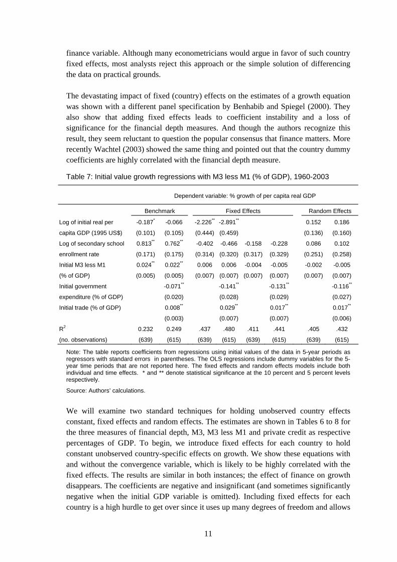
finance variable. Although many econometricians would argue in favor of such country fixed effects, most analysts reject this approach or the simple solution of differencing the data on practical grounds. The devastating impact of fixed (country) effects on the estimates of a growth equation was shown with a different panel specification by Benhabib and Spiegel (2000). They also show that adding fixed effects leads to coefficient instability and a loss of significance for the financial depth measures. And though the authors recognize this result, they seem reluctant to question the popular consensus that finance matters. More recently Wachtel (2003) showed the same thing and pointed out that the country dummy coefficients are highly correlated with the financial depth measure.

Table 7: Initial value growth regressions with M3 less M1 (% of GDP), 1960-2003





-0.187*

(0.101)

-0.066

(0.105)

-2.226**

(0.444)

-2.891**

(0.459)

0.152

(0.136)

0.186

(0.160)


enrollment rate

0.813**

(0.171)

0.762**

(0.175)

-0.402

(0.314)

-0.466

(0.320)

-0.158

(0.317)

-0.228

(0.329)

0.086

(0.251)

0.102

(0.258)

Initial M3 less M1

(% of GDP)

0.024**

(0.005)

0.022**

(0.005)

0.006

(0.007)

0.006

(0.007)

-0.004

(0.007)

-0.005

(0.007)

-0.002

(0.007)

-0.005

(0.007)

Initial government

expenditure (% of GDP)

-0.071**

(0.020)

-0.141**

(0.028)

-0.131**

(0.029)

-0.116**

(0.027)


(0.003)

0.029**

(0.007)

0.017**

(0.007)

0.017**

(0.006)

R2

(no. observations)

0.232

(639)

0.249

(615)

.437

(639)

.480

(615)

.411

(639)

.441

(615)

.405

(639)

.432

(615)

Note: The table reports coefficients from regressions using initial values of the data in 5-year periods as regressors with standard errors in parentheses. The OLS regressions include dummy variables for the 5-year time periods that are not reported here. The fixed effects and random effects models include both individual and time effects. * and ** denote statistical significance at the 10 percent and 5 percent levels respectively.


We will examine two standard techniques for holding unobserved country effects constant, fixed effects and random effects. The estimates are shown in Tables 6 to 8 for the three measures of financial depth, M3, M3 less M1 and private credit as respective percentages of GDP. To begin, we introduce fixed effects for each country to hold constant unobserved country-specific effects on growth. We show these equations with and without the convergence variable, which is likely to be highly correlated with the fixed effects. The results are similar in both instances; the effect of finance on growth disappears. The coefficients are negative and insignificant (and sometimes significantly negative when the initial GDP variable is omitted). Including fixed effects for each country is a high hurdle to get over since it uses up many degrees of freedom and allows

12

the dummies to pick up all country specific differences. A less demanding hurdle is provided by the random effects model, which allows for a country specific component in the regression error term. Estimates with random effects are shown in the last two columns of Tables 6 to 8. The effect on the coefficients on financial depth is dramatic in the random effects model as well. As with fixed effects, the coefficients are negative and not statistically significant.

Table 8: Initial value growth regressions with private sector credit (% of GDP), 1960-2003





-0.094

(0.110)

0.005

(0.113)

-1.954**

(0.444)

-2.609**

(0.455)

0.229*

(0.134)

0.231

(0.158)


enrollment rate

0.899**

(0.170)

0.842**

(0.173)

-0.335

(0.310)

-0.392

(0.316)

-0.155

(0.312)

-0.207

(0.324)

0.089

(0.245)

0.114

(0.253)

Initial private sector

credit (% of GDP)

0.007*

(0.004)

0.006

(0.004)

-0.006

(0.006)

-0.004

(0.006)

-0.016**

(0.006)

-0.016**

(0.006)

-0.015**

(0.005)

-0.017**

(0.005)

Initial government

expenditure (% of GDP)

-0.069**

(0.019)

-0.131**

(0.027)

-0.124**

(0.027)

-0.112**

(0.026)


(0.003)

0.030**

(0.007)

0.021**

(0.007)

0.020**

(0.006)

R2

(no. observations)

0.200

(667)

0.224

(643)

.428

(667)

.472

(643)

.416

(653)

.440

(643)

.401

(667)

.431

(643)

Note: The table reports coefficients from regressions using initial values of the data in 5-year periods as regressors with standard errors in parentheses. The OLS regressions also include dummy variables for the 5-year time periods. The fixed effects and random effects models include both individual and time effects. * and ** denote statistical significance at the 10 percent and 5 percent levels respectively.


Proponents of the standard growth rate equation would argue that the specification does not call for country fixed effects. The equation is derived from a production function relationship and so the country-specific unobserved effects disappear with the differencing. Whether fixed or random effects should be in the growth equation can be debated. The point is that these results are troubling. We have shown that the finance coefficient, which seems so robust and invariant in the baseline results, is sensitive to the time period for estimation and disappears entirely when we hold country-specific variations constant with either random or fixed effects. The core problem is to determine whether we are observing differences among countries or causality from financial depth to growth. Do estimates of (1) with appropriate econometric technique

13

Figure 1: Histograms of the three measures of financial depth by country

13

14

reflect causality from F to Y or summarize the idiosyncrasies of countries? The distinction is important because the former has strong policy lessons while the latter does not. A common source of sample composition problems is the role of outliers. As shown in Figure 1, the distributions of the financial depth measures by country are highly skewed with just a few countries exhibiting much higher levels of financial depth than the others.11 The high ratios of credit or M3 to GDP in Japan and Switzerland in panel (a) of Figure 1, for example, are the consequence of idiosyncratic capital structure of industry in one case and the prominence of the financial services sector in the other. Estimates of equation (1) with the outlier observations excluded (not shown here) indicate some sensitivity to their presence. Any one country has too few observations to substantially affect the statistical significance of a result observed in the aggregate data sample. However, there are changes in the size of the coefficients on financial depth when one or two outlier countries are removed.12 To examine the effects of sample composition more systematically we utilize the rolling regression techniques first applied to study of the finance–growth nexus by Rousseau and Wachtel (2002). Figure 2 presents results from two rolling IV regression experiments that use the simple baseline equation with the M3 ratio as the finance variable.13 We focus on the M3 ratio in this part of the analysis because it produces results that are representative of those obtained with the other two finance measures. The two panels in the figure present the coefficients on the finance variable for different ways of rolling in observations. The left and right hand pictures in each panel show the coefficients with alternative metrics along the horizontal axis. In each picture the estimated coefficients are given by the solid line and 5 percent confidence intervals are given by the dotted lines. In panel (a) we order the countries by the average level of financial depth (after adjusting for global time effects) and roll them in as the ratio of M3 to GDP increases. The initial regression includes the 20 countries with the lowest levels of financial depth and rolls in additional countries one by one. The results are presented in two ways. The left hand picture shows the evolution of the finance coefficient as the number of countries increases from 20 to 84. The picture on the right hand side shows the same coefficients graphed against the M3 ratio for the last country rolled in (it is about 40 percent for the largest of the first 20 counties and increases to over 160 percent when Malta is rolled in last).

11 To construct the histograms, we regress 5-year averages of the financial depth measures for all of the countries in our sample on a constant and on dummy variables for the time periods. The histograms then include averages of the adjusted series for each country (i.e., the residuals with the constant term added back in). 12 Manning (2003) shows that the influence of the Asian tiger countries may be driving empirical results on the finance growth relationship in a different modeling context. 13 The overall estimate for the entire sample is equation 1 in Table 1.

15

Figure 2: Evolution of coefficients on M3 (% GDP) in cross-country rolling regressions 1960-2003

(a) countries ordered by increasing M3 (% of GDP)

(b) countries ordered by decreasing M3 (% of GDP) The financial effect is negative for the countries with the least developed financial sectors and does not cross the zero line until about 30 countries are included in the regression. More importantly, the financial effect is not significantly different from zero until about 65 of 84 countries are included or the ratio of M3 to GDP reaches 70 percent. Apparently it is the comparison of less developed countries to more developed ones that is responsible for the observed effect. Somewhat different results are found in the panel (b), which shows the finance coefficients when countries are rolled into the regression by decreasing rather than increasing size of the M3/GDP ratio.14 In panel (b) the coefficient starts positive and

14 Note that the endpoints for panel (a) and (b), when all countries are rolled into the regression, are the same.

16

just about significantly different from zero. Because the distribution of the M3 ratio is skewed, there is lots of variation among the 20 countries with the most financial depth and many large, fast growing countries with well-developed financial sectors throughout (e.g. the US) are in the sample. This serves to suggest once again that the country effects dominate the causality that we are looking for. A drawback of these rolling regressions is that the sample size varies as we move along the graph. To avoid that, we present rolling regressions with a constant 20-country window in Figure 3.15 The top panel of Figure 3 shows the coefficients on financial depth with countries rolled in as the ratio of M3 to GDP increases. Thus, the first observation on the graphs is the coefficient from a regression that includes the 20 countries with the smallest financial depth ratios and the last observation is from the regression with the 20 countries with the largest ratios. As before, the financial depth coefficients are shown in two ways, by country and by size of the M3/GDP ratio. All along these figures, we are looking at regressions using data from 20 countries with relatively homogenous financial sectors. If there were causality from finance to growth we would expect to find it with these regressions as we examine small perturbations across time and country in financial depth. Among the financially less developed countries the coefficient is sometimes negative, is quite variable, and is imprecisely measured. Among the financially most developed countries the coefficient is about zero; although financial depth differs a lot among these countries (note the skewness of the distribution in Figure 1), it has no relationship to growth. However, there is some indication of a positive relationship in the middle ranges, countries with M3 to GDP ratios between 45 and 60 percent. For these countries increased financial depth has a strong effect on growth that is almost significant at the 5 percent level. The next panel in Figure 3 provides additional evidence of a finance–growth relationship for certain countries. It shows results from rolling regressions with a 20-country window where countries are rolled in by increasing average per capita income (in 1995 US$).16 For very low-income countries (income below US$3,000), the effect of financial deepening is positive but not significant. The effect is imprecisely estimated because in many of these countries increased financial depth might be due to directed finance and poor lending standards. However, in the middle income range (from US$3,000 to US$12,000) there seems to be clear evidence of a finance growth relationship. At these income levels, groups of countries that are relatively homogeneous by income have different growth experiences that are related to financial

15 Note that there are many more than 20 observations in each regression because there are as many as nine time period observations for each of the 20 countries. 16 We establish an income ordering of countries by regressing the initial values of per capita income in each 5-year period for all of the countries in our sample on a constant term and dummy variables for the time periods. We then use the averages of the adjusted series for each country (i.e., the residuals with the constant term added back in).

17

depth. The relationship disappears among higher income countries with the coefficients around zero.17 These results suggest that there might be some life yet to the finance growth nexus.

Figure 3: Evolution of coefficients on M3 (% GDP) in rolling window cross-country regressions 1960-2003

(a) 20-country rolling window ordered by increasing M3 (% of GDP)

(b) 20-country rolling window order by increasing per capita income (thousands of 1995 US$)

17 Deidda and Fattouh (2002) reach a different conclusion with threshold regression estimates with the King and Levine data for 1960 to 1989. They find that the finance effect on growth is weak in low income countries.

18

Conclusion

In this paper we examine the robustness of some now classic findings on the cross-country relationship between financial development and economic growth. Though we find the relationship to be robust to our choice of conditioning variables and econometric technique, our main findings offer good reason for pause. The finance–growth relationship that has seemed so robust in studies using data from the 1960s to the 1980s simply does not carry over to data from the past fifteen years. Further, the usual results disappear when fixed or random effects for countries are included in the specifications, suggesting that the measures of financial depth in the standard growth equation may be standing in for other unobserved country-specific factors. The sensitivity of the standard findings to the removal of countries that appear to be outliers also hints at the importance of such country effects. Our findings are in some ways reminiscent of Robert Lucas’s famous critique of econometric policy evaluation advanced nearly three decades ago. In Lucas (1975) the focus was on the now-obvious misuse of the Phillips curve in formulating policy prescriptions, but the basic lesson may apply in our application as well. In particular, policies that have promoted and/or forced increases in financial depth over the past two decades, perhaps in response to the prevailing Washington consensus, may well have altered the basic structural relationship between finance and growth. It would then be inappropriate to use the coefficients on finance obtained with data before 1990 (i.e., prior to the widespread acceptance of the finance–growth relationship) to estimate the impact of future policy initiatives aimed at spurring growth through increasing the size of a country’s financial sector. Yet many emerging economies around the world did exactly that. The devastating effects of premature financial liberalizations operating through the increased volatility of international capital flows on the emerging East Asian economies in the late 1990’s are just a few cases in point. All of this does not detract from the basic point that at one time countries with higher levels of financial development tended to have higher growth rates than those with lower levels of financial development. The question of how these countries acquired large financial sectors and how they may have served as engines of growth, however, remains imperfectly understood. Did finance emerge due to the presence of deeper institutional fundamentals that had a direct impact on growth as Acemoglu, Johnson, and Robinson (2001) suggest? Or is Joan Robinson (1952) correct that growth is the prime mover behind financial development? Our study, while by no means arguing that financial factors are unimportant for economic development, serves simply as a reminder that the correlations between finance and growth found in cross-country data may well reflect differences in country characteristics rather than any dynamic cause-effect relationship from finance to growth. If this is the case, the systematic study of the financial development experiences of individual countries becomes all the more critical as the next step in furthering our understanding of the nexus.

19

References

Acemoglu, Daron, Simon Johnson, and James A. Robinson (2001). ‘The colonial origins of economic development: an empirical investigation’, American Economic Review 91: 1369-401.

Arellano, Manuel, and Stephen Bond (1991). ‘Some tests of specification for panel data: Monte Carlo evidence and an application to employment fluctuations’, Review of Economic Studies 58: 277-97.

Arestis, Philip, and Panicos O. Demetriades (1997). ‘Financial development and economic growth: assessing the evidence’, Economic Journal 107: 783-99.

Arestis, Philip, Panicos O. Demetriades, and Kul B. Luintel (2001). ‘Financial development and economic growth: the role of stock markets’, Journal of Money, Credit, and Banking 33: 16-41.

Barro, Robert J. (1991). ‘Economic growth in a cross section of countries’, Quarterly Journal of Economics 106: 407-43.

Benhabib, Jess, and Mark M. Spiegel (1994). ‘The role of human capital in economic development: evidence from aggregate cross-country data’, Journal of Monetary Economics 34: 143-73.

Deidda, Luca, and Bassam Fattouh (2002). ‘Non-linearity between finance and growth’, Economic Letters 74: 339-45.

Demetriades, Panicos O., and Khaled A. Hussein (1996). ‘Does financial development cause economic growth? Time series evidence from sixteen countries’, Journal of Development Economics 51: 387-411.

Goldsmith, Raymond W. (1969). Financial structure and development, Yale University Press: New Haven CT. University Press.

King, Robert G., and Ross Levine (1993). ‘Finance and growth: Schumpeter might be right’, Quarterly Journal of Economics 108: 717-37.

Levine, Ross (1997). ‘Financial development and economic growth: views and agenda’. Journal of Economic Literature 35: 688-726.

Levine, Ross (2005). ‘Finance and growth: theory and evidence’, forthcoming in P. Aghion and S.N. Durlauf (eds), Handbook of Economic Growth, North Holland: Amsterdam.

Levine, Ross, Norman Loayza, and Thorsten Beck (2000). Financial intermediation and growth: causality and causes. Journal of Monetary Economics 46: 31-77.

Levine, Ross and David Renelt (1992). ‘A sensitivity analysis of cross-country growth regressions’, American Economic Review 84: 942-63.

20

Levine, Ross and Sara Zervos (1998). Stock markets, banks, and economic growth, American Economic Review 88: 537-58.

Lucas, Robert E., Jr. (1975). ‘Econometric policy evaluation: a critique’, Carnegie-Rochester Series on Public Policy 1: 19-46.

Lucas, Robert E., Jr. (1988). ‘On the mechanics of economic development’, Journal of Monetary Economics 22: 3-42.

Manning, Mark J. (2003). ‘Finance causes growth: can we be so sure?’, Contributions to Macroeconomics 3 www.bepress.com/bejm/contributions/vol3/iss1/art12

McKinnon, R.I., (1973). Money and Capital in Economic Development, The Brookings Institution: Washington DC.

McKinnon, R.I., (1991). The Order of Economic Liberalization, The Johns Hopkins University Press: Baltimore and London.

Rioja, Felix, and Neven Valev (2004). ‘Does one size fit all? A re-examination of the finance and growth relationship’, Journal of Development Economics 74: 429-47.

Robinson, Joan (1952). ‘The generalization of the general theory’, in The Rate of Interest and Other Essays, Macmillan: London.

Rousseau, Peter L., and Paul Wachtel (1998). ‘Financial intermediation and economic performance: historical evidence from five industrialized countries’, Journal of Money, Credit and Banking 30: 657-78.

Rousseau, Peter L., and Paul Wachtel (2000). ‘Equity markets and growth: cross-country evidence on timing and outcomes, 1980-1995’, Journal of Banking and Finance 24: 1933-57.

Rousseau, Peter L., and Paul Wachtel (2002). Inflation thresholds and the finance–growth nexus’, Journal of International Money and Finance 21: 277-93.

Temple, Jonathan (1999). ‘The new growth evidence’, Journal of Economic Literature 37: (March), 112-56.

Wachtel, Paul (2003). ‘How much do we really know about growth and finance?’, Federal Reserve Bank of Atlanta Economic Review 88: 33-47.

Documents

Economic Growth and Financial Depth - UNU-WIDER€¦ · · 2015-08-18advocacy of policies leading ... country and panel datasets for the post-1960 period.2 The influence of financial