Economic Growth and Evolution of Gender Equality∗

Tatiana Damjanovic † Geethanjali Selvaretnam‡

Abstract

We put forward a theoretical growth model where the degree of gender equality

evolves towards the value maximising social output. It follows that a woman’s

bargaining power positively depends on her relative productivity. When an economy

is less developed, physical strength is quite important for production and therefore

the total output is bigger when the man has larger share of the reward. As society

develops and accumulates physical and human capital, the woman becomes more

productive, which drives social norms towards gender equality. By endogenising

gender balance of power we can explain why it differs across societies and how it

evolves over the time.

Key Words: gender inequality, economic growth, female bargaining power,

human capital, natural resources

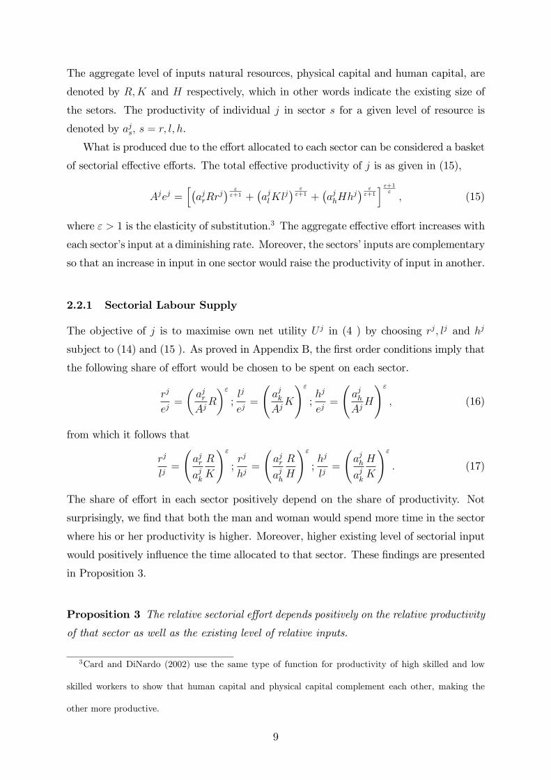
JEL: C72, C73, D13, J16, O41, O43

∗Acknowledgements: We thank seminar participants at the University of St Andrews, especially

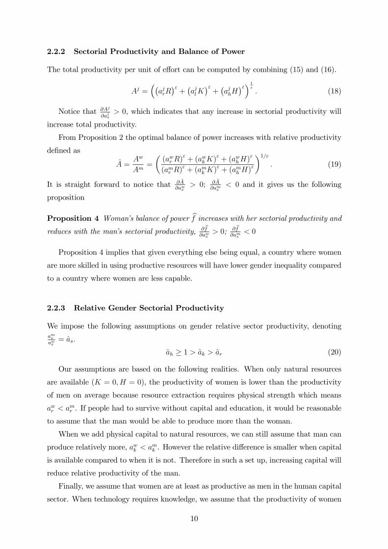
David Ulph, Paola Manzini, Radoslaw Stefanski, Ian Smith and Helmut Rainer for helpful comments

and discussions. The usual disclaimer applies.†Business School, Durham University Stockton Road, Durham, DH1 3LE; Tel: 0044 (0)191 33 45198;

email: tatiana.damjanovic@durham.ac.uk‡Adam Smith Business School, University of Glasgow, G12 8QQ; Tel: 0044 (0)141 330 4496; email:

Geethanjali.Selvaretnam@glasgow.ac.uk

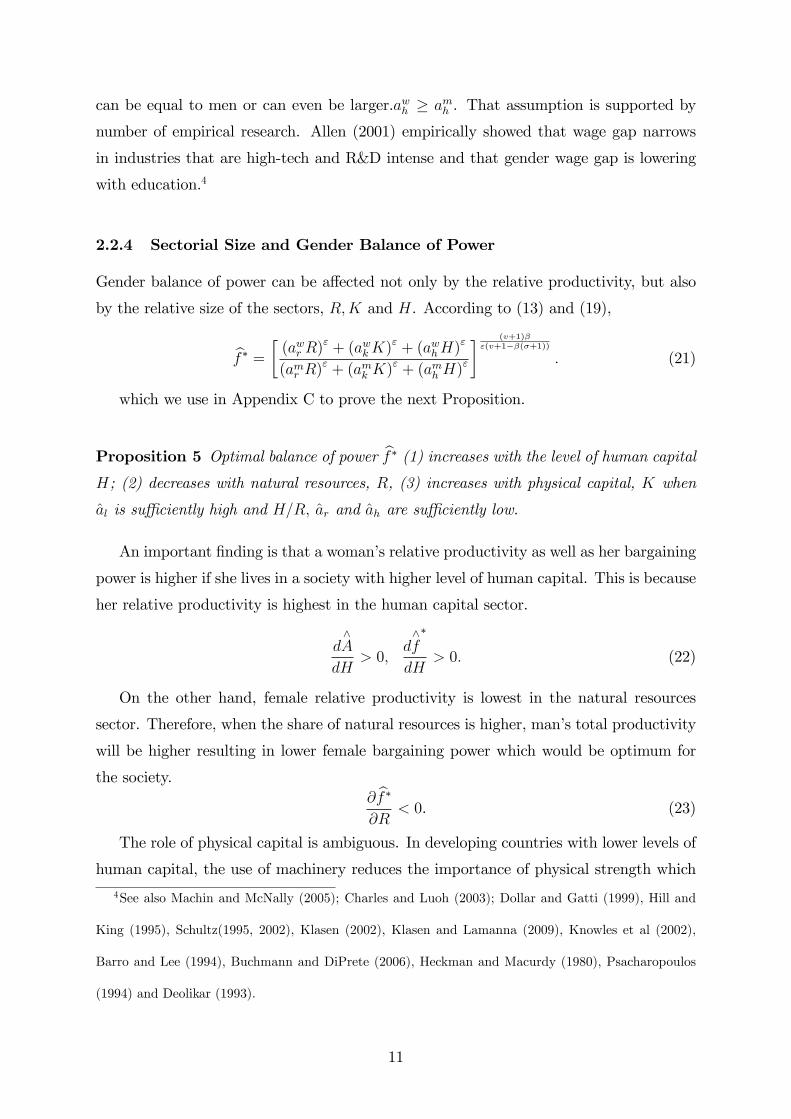
1

1 Introduction

Gender balance of power in a society is regulated by many institutions such as social

norms, religious traditions and legal regulations. These institutions not only vary across

countries but also change over history. Our paper proposes a growth model explaining

evolution of gender equality

We will use a popular assumption that social institutions evolve towards the largest

probability of survival. This idea was formulated by behaviour biologists (Hamilton 1964,

Levin and Kimer, 1974) and has been accepted and developed by economists (Frank,

1998; Bergstrom, 1995; Alger and Weibull, 2010, 2012). Ceteris paribus, a society which

produces larger economic output can afford a stronger defence and will survive with a

larger probability in a hostile environment. Its institutions are also more attractive for

imitation by other communities. Therefore, it is reasonable to assume that social norms

evolve towards those which maximise the social output. We apply that concept to explain

the evolution of gender balance of power.

Women have been subjected to many forms of discrimination within the family,

workplace and society throughout history. This discrimination can start even before

birth in some regions where boys are preferred to girls for various reasons, resulting

in sex selective abortions and deaths of baby girls (Bhaskar and Gupta, 2007; Edlund

and Lee, 2013; Almond et al, 2009). Many religions and cultures encourage women

to be subservient to men. This is implicitly reflected in the evidence of domestic abuse.

Borooah andMangan (2009) found that women are eight times more likely to be subjected

to spousal attacks in Australia and six times more likely in Canada. Kury et al (2004)

compare domestic violence across Europe and say that the variation is explained by

general tolerance towards domestic violence, economic conditions and cultural outlook

on women and their position.

An increasing trend in women’s position in society, labour market and family during

the last century has been observed and documented in academic literature and it has

been shown that gender wage gap has significantly decreased [Blau, 1998; Edin and

Richardson, 2002; Goldin, 2006; Mulligan and Rubinstein, 2008; Heathcote et al., 2010.

According to Dugan et al (1998) domestic homicide rate has been reduced in the US

over the past 25 years. Farmer and Tiefenthaler (2003) empirically show that increase in

economic conditions of women and better legal provision for victims have played a role

in the reduction of domestic violence over the recent past.

Although female balance of power has increased over time, its level and the rate of

2

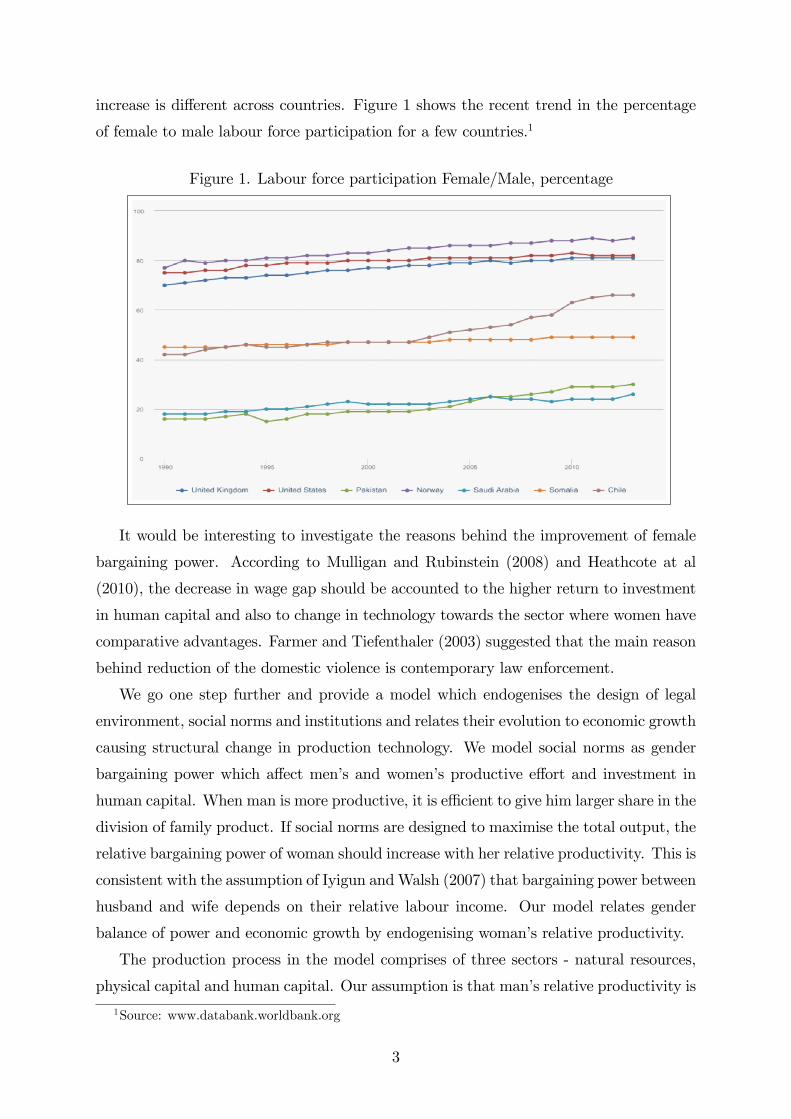
increase is different across countries. Figure 1 shows the recent trend in the percentage

of female to male labour force participation for a few countries.1

Figure 1. Labour force participation Female/Male, percentage

It would be interesting to investigate the reasons behind the improvement of female

bargaining power. According to Mulligan and Rubinstein (2008) and Heathcote at al

(2010), the decrease in wage gap should be accounted to the higher return to investment

in human capital and also to change in technology towards the sector where women have

comparative advantages. Farmer and Tiefenthaler (2003) suggested that the main reason

behind reduction of the domestic violence is contemporary law enforcement.

We go one step further and provide a model which endogenises the design of legal

environment, social norms and institutions and relates their evolution to economic growth

causing structural change in production technology. We model social norms as gender

bargaining power which affect men’s and women’s productive effort and investment in

human capital. When man is more productive, it is effi cient to give him larger share in the

division of family product. If social norms are designed to maximise the total output, the

relative bargaining power of woman should increase with her relative productivity. This is

consistent with the assumption of Iyigun andWalsh (2007) that bargaining power between

husband and wife depends on their relative labour income. Our model relates gender

balance of power and economic growth by endogenising woman’s relative productivity.

The production process in the model comprises of three sectors - natural resources,

physical capital and human capital. Our assumption is that man’s relative productivity is

1Source: www.databank.worldbank.org

3

very high in resource extraction sector but it declines when physical capital accumulated.

Furthermore, we assume that the marginal productivity of a woman with respect to

human capital is not less than that of a man. The level and composition of the three

production sectors change over time. In the early days of civilization, male physical

strength was very important in resource extraction. As technology improved, his relative

productivity declines and therefore the social institution evolved towards lower gender

inequality. That in turn, incentivises female education and labour market participation.

Over time, as human capital accumulates, total production keeps increasing and relative

productivity of man declines, which increases female bargaining power. So long as human

capital productivity is the same for both man and woman, gender balance of power will

converge to equality.

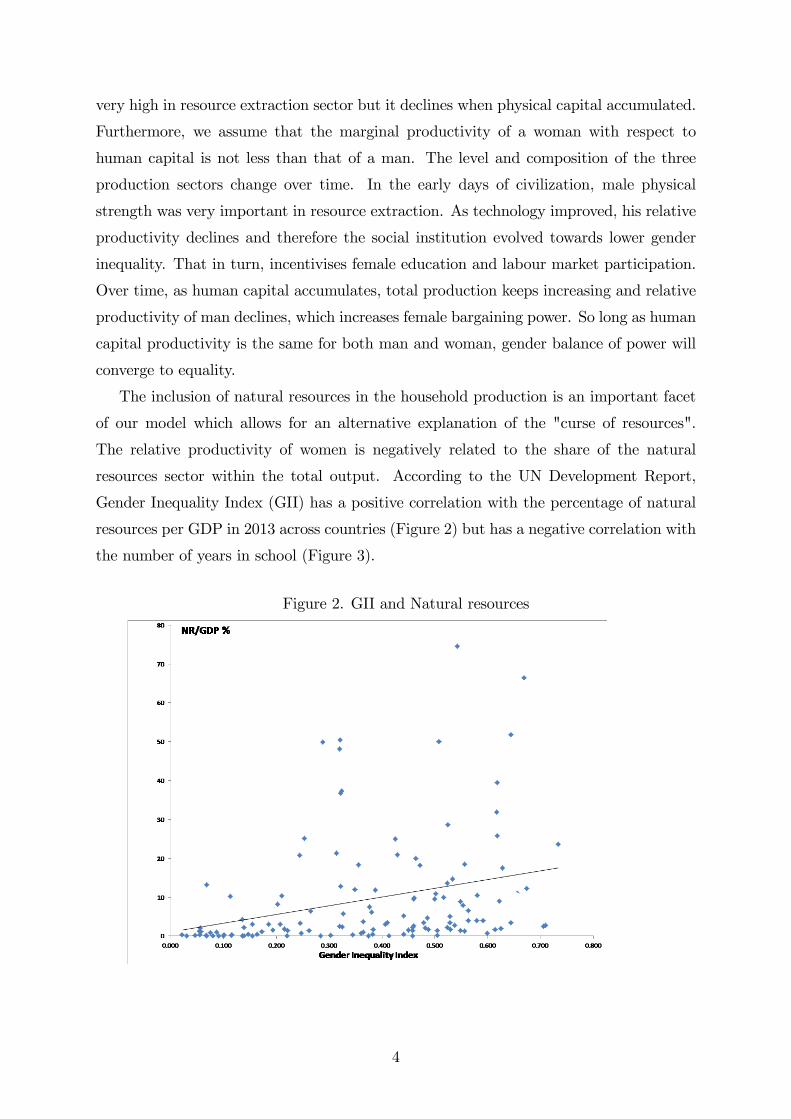
The inclusion of natural resources in the household production is an important facet

of our model which allows for an alternative explanation of the "curse of resources".

The relative productivity of women is negatively related to the share of the natural

resources sector within the total output. According to the UN Development Report,

Gender Inequality Index (GII) has a positive correlation with the percentage of natural

resources per GDP in 2013 across countries (Figure 2) but has a negative correlation with

the number of years in school (Figure 3).

Figure 2. GII and Natural resources

4

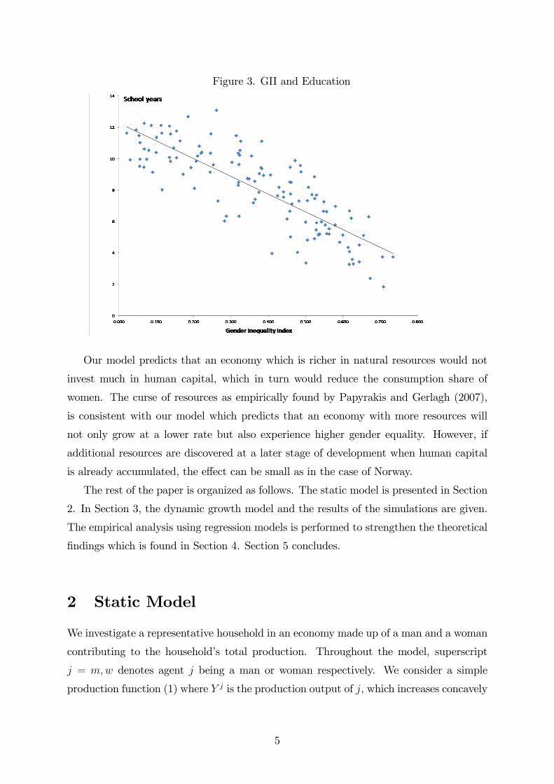
Figure 3. GII and Education

Our model predicts that an economy which is richer in natural resources would not

invest much in human capital, which in turn would reduce the consumption share of

women. The curse of resources as empirically found by Papyrakis and Gerlagh (2007),

is consistent with our model which predicts that an economy with more resources will

not only grow at a lower rate but also experience higher gender equality. However, if

additional resources are discovered at a later stage of development when human capital

is already accumulated, the effect can be small as in the case of Norway.

The rest of the paper is organized as follows. The static model is presented in Section

2. In Section 3, the dynamic growth model and the results of the simulations are given.

The empirical analysis using regression models is performed to strengthen the theoretical

findings which is found in Section 4. Section 5 concludes.

2 Static Model

We investigate a representative household in an economy made up of a man and a woman

contributing to the household’s total production. Throughout the model, superscript

j = m,w denotes agent j being a man or woman respectively. We consider a simple

production function (1) where Y j is the production output of j, which increases concavely

5

with effort ej. The term Aj captures some parameters which influence the productivity.

Y j =(Ajej

)β, (1)

where β < 1 is effort elasticity of production. The joint family income of the household

is given by Y,

Y = Y m + Y w. (2)

Each agent j receives a proportion f j ∈ [0, 1] of the total household production forconsumption (fw + fm = 1). This proportion is determined by the bargaining power of

w and m which is generally accepted as the social norm

Cj = f jY. (3)

Net utility of j is U j. It increases with consumption, Cj, and decreases with effort, ej.

U j = u(Cj)− V (ej), (4)

where uC > 0 and uCC < 0. Furthermore, we assume that 0 < −CuCCuc

< 1, so

that j’s relative risk aversion is between zero and one. Disutility of effort is convex:

Ve > 0, Vee > 0, Veee > 0. We assume the following functional forms for the purpose of

our analysis and simulations

u =Cσ

σ; V =

e1+v

1 + v. (5)

where 0 < σ ≤ 1 and v ≥ 1.

2.1 Bargaining Power and Production

Decision problems are the same for both the man and woman who are similar in everything

except for their productivity and bargaining power. Given fw, the woman maximises her

utility by choosing the level of effort as shown in (6).2

Maxew

u [fw (Y w (ew) + Y m)]− V (ew). (6)

The first order condition given by (7) defines the woman’s supply of effort

fwuC (fwY )Y w

ew − Vew = 0. (7)

2The second order condition is satisfied because ujCC , YjeW eW

< 0.

f2uwCCYwewY

wew + fu

wc Y

wewew − V wewew < 0.

6

The man’s decision is similar. Applying the implicit function theorem to condition (7)

we can prove that the woman’s effort increases with her bargaining power. However we

cannot increase the bargaining power of woman without decreasing that of the man’s.

The social return on extra effort ej depends on the productivity Aj and we expect that

output maximising solution would be to give a larger share to a more productive person.

We can check it formally.

Given the effort supply decisions of m and w, we calculate fw which would maximise

social product Y . The first order conditions imply the following proposition.

Proposition 1 The optimal relative bargaining power is equal to the relative output,fw

fm= Y w

Ym.

Proof. See Appendix A

Proposition 1 states that the man’s share should be larger when his relative output

is higher. It is optimal on the whole to give a higher share to the agent who is more

productive to encourage higher production.

For further reference, it is convenient to define relative parameters. Let∧e, A, Y and

f be the woman’s relative choice of effort, productivity, production and balance of power

respectively.∧e =

ew

em; A =

Aw

Am; Y =

Y w

Y m; f =

f

1− f . (8)

Notice that Proposition 1 presents only the partial equilibrium result as the production

of the man and woman are endogenous to their choice of effort. The effort supply

equations implyfwuc (f

wY )Y we e

w

fmuc (fmY )Y me e

m=V we e

w

V me e

m, (9)

which for the constant elasticity functional forms (5) gives(f)σY = (e)v+1 . (10)

Combining it with production function (1), we get relative effort and relative output as

a function of relative productivity and gender inequality.

e =(A) βv+1−β

(f) σv+1−β

. (11)

Y =(A)β(v+1)v+1−β

(f) βσv+1−β

. (12)

As expected, d∧e

df> 0. When the share obtained by the woman increases, it has a

positive effect on her effort and a negative effect on the man’s effort, ewf > 0, emf < 0.

7

Using Proposition 1 and (12) optimum balance of power can be written as

f ∗ =(A) β(v+1)(v+1)−β(σ+1)

. (13)

The optimum balance of power is what would maximise total production. An

important observation from this result is that the relative share received by j positively

depend on j’s relative productivity, df∗

dA> 0. When the man is given more power (i.e.

when f is low), it will incentivise him to put in more effort, but it will discourage the

woman. So long as the increase in his production is higher than the decrease in the

woman’s production, the total production will be higher. We can therefore conclude that

when the relative productivity A is lower, f ∗ would be lower, as stated in Proposition 2.

Proposition 2 An increase in relative productivity results in higher relative effort,

relative production and balance of power.

2.2 Structural Composition

Now we will explain the difference in productivity between man and woman. Our

production process consists of three sectors. The first, natural resource sector, uses

available natural resources and manual labour. This includes hunting, fishing, gathering

fruits and vegetables, building shelter, weaving etc. Here we also include extraction of the

natural resources such as oil and minerals. The second, physical capital sector, produces

with the aid of machinery. Finally, human capital sector, produces using creativity and

brain power, rather than physical strength. Activities which fall into this category would

not only be those such as the high-tech industry, financial services etc., but also effi cient

organisation of daily activities, management, creative work, art and entertainment etc.

We will assume that female relative productivity is highest in the human capital

sector. As the economy develops, human capital accumulates and this sector becomes

more important in production. That causes an increase in female relative productivity,

and consequently on female bargaining power.

We consider effort ej to be devoted by j to the production in each of these sectors,

namely natural resource, physical capital and human capital denoted by rj, lj and hj

respectively.

ej = rj + lj + hj (14)

The total productivity of j in each given sector depends on the existing level of

resources in the whole economy as well as j’s own productivity in that particular sector.

8

The aggregate level of inputs natural resources, physical capital and human capital, are

denoted by R,K and H respectively, which in other words indicate the existing size of

the setors. The productivity of individual j in sector s for a given level of resource is

denoted by ajs, s = r, l, h.

What is produced due to the effort allocated to each sector can be considered a basket

of sectorial effective efforts. The total effective productivity of j is as given in (15),

Ajej =[(ajrRr

j) εε+1 +

(ajlKl

j) εε+1 +

(ajhHh

j) εε+1

] ε+1ε, (15)

where ε > 1 is the elasticity of substitution.3 The aggregate effective effort increases with

each sector’s input at a diminishing rate. Moreover, the sectors’inputs are complementary

so that an increase in input in one sector would raise the productivity of input in another.

2.2.1 Sectorial Labour Supply

The objective of j is to maximise own net utility U j in (4 ) by choosing rj, lj and hj

subject to (14) and (15 ). As proved in Appendix B, the first order conditions imply that

the following share of effort would be chosen to be spent on each sector.

rj

ej=

(ajrAjR

)ε;lj

ej=

(ajkAjK

)ε

;hj

ej=

(ajhAjH

)ε

, (16)

from which it follows that

rj

lj=

(ajrajk

R

K

)ε

;rj

hj=

(ajrajh

R

H

)ε

;hj

lj=

(ajhajk

H

K

)ε

. (17)

The share of effort in each sector positively depend on the share of productivity. Not

surprisingly, we find that both the man and woman would spend more time in the sector

where his or her productivity is higher. Moreover, higher existing level of sectorial input

would positively influence the time allocated to that sector. These findings are presented

in Proposition 3.

Proposition 3 The relative sectorial effort depends positively on the relative productivity

of that sector as well as the existing level of relative inputs.

3Card and DiNardo (2002) use the same type of function for productivity of high skilled and low

skilled workers to show that human capital and physical capital complement each other, making the

other more productive.

9

2.2.2 Sectorial Productivity and Balance of Power

The total productivity per unit of effort can be computed by combining (15) and (16).

Aj =((ajrR

)ε+(ajlK

)ε+(ajhH

)ε) 1ε. (18)

Notice that ∂Aj

∂ajs> 0, which indicates that any increase in sectorial productivity will

increase total productivity.

From Proposition 2 the optimal balance of power increases with relative productivity

defined as

A =Aw

Am=

((awr R)

ε + (awkK)ε + (awhH)

ε

(amr R)ε + (amk K)

ε + (amh H)ε

)1/ε. (19)

It is straight forward to notice that ∂A∂aws

> 0; ∂A∂ams

< 0 and it gives us the following

proposition

Proposition 4 Woman’s balance of power f increases with her sectorial productivity and

reduces with the man’s sectorial productivity, ∂f∂aws

> 0; ∂f∂ams

< 0

Proposition 4 implies that given everything else being equal, a country where women

are more skilled in using productive resources will have lower gender inequality compared

to a country where women are less capable.

2.2.3 Relative Gender Sectorial Productivity

We impose the following assumptions on gender relative sector productivity, denotingamsaws= as.

ah ≥ 1 > ak > ar (20)

Our assumptions are based on the following realities. When only natural resources

are available (K = 0, H = 0), the productivity of women is lower than the productivity

of men on average because resource extraction requires physical strength which means

awr < amr . If people had to survive without capital and education, it would be reasonable

to assume that the man would be able to produce more than the woman.

When we add physical capital to natural resources, we can still assume that man can

produce relatively more, awk < amk . However the relative difference is smaller when capital

is available compared to when it is not. Therefore in such a set up, increasing capital will

reduce relative productivity of the man.

Finally, we assume that women are at least as productive as men in the human capital

sector. When technology requires knowledge, we assume that the productivity of women

10

can be equal to men or can even be larger.awh ≥ amh . That assumption is supported by

number of empirical research. Allen (2001) empirically showed that wage gap narrows

in industries that are high-tech and R&D intense and that gender wage gap is lowering

with education.4

2.2.4 Sectorial Size and Gender Balance of Power

Gender balance of power can be affected not only by the relative productivity, but also

by the relative size of the sectors, R,K and H. According to (13) and (19),

f ∗ =

[(awr R)

ε + (awkK)ε + (awhH)

ε

(amr R)ε + (amk K)

ε + (amh H)ε

] (v+1)βε(v+1−β(σ+1))

. (21)

which we use in Appendix C to prove the next Proposition.

Proposition 5 Optimal balance of power f ∗ (1) increases with the level of human capital

H; (2) decreases with natural resources, R, (3) increases with physical capital, K when

al is suffi ciently high and H/R, ar and ah are suffi ciently low.

An important finding is that a woman’s relative productivity as well as her bargaining

power is higher if she lives in a society with higher level of human capital. This is because

her relative productivity is highest in the human capital sector.

d∧A

dH> 0,

d∧f∗

dH> 0. (22)

On the other hand, female relative productivity is lowest in the natural resources

sector. Therefore, when the share of natural resources is higher, man’s total productivity

will be higher resulting in lower female bargaining power which would be optimum for

the society.∂f ∗

∂R< 0. (23)

The role of physical capital is ambiguous. In developing countries with lower levels of

human capital, the use of machinery reduces the importance of physical strength which

4See also Machin and McNally (2005); Charles and Luoh (2003); Dollar and Gatti (1999), Hill and

King (1995), Schultz(1995, 2002), Klasen (2002), Klasen and Lamanna (2009), Knowles et al (2002),

Barro and Lee (1994), Buchmann and DiPrete (2006), Heckman and Macurdy (1980), Psacharopoulos

(1994) and Deolikar (1993).

11

reduces the relative productivity of men. When human capital to natural resource ratio

is low, accumulation of physical capital will empower women. However, in a society with

relatively high level of human capital, extra physical capital may reduce female bargaining

power.∂f ∗

∂K> 0 if

H

R<

[((al)

ε − (ar)ε)((ah)

ε − (al)ε)

]1/εamramh

. (24)

3 Dynamic Model

Now that we have analysed how a representative man and woman allocate their effort

in a static model, we would like to investigate how this set up affects the production in

successive periods. We use a simple growth model to analyse this issue within a dynamic

framework.

The physical capital changes over time as in Solow (1956)

Kt+1 = (1− δ)Kt + ϕYt, (25)

where δ is the rate of depreciation and ϕ is the proportion of output which is saved and

invested into capital.

Human capital accumulates according to Becker et al (1990)

Ht+1 = Ht + ω (hwt + hmt )1−θ (Ht)

θ (26)

where the investment in human capital, hjt , is chosen by j in period t according to the

decision problem introduced in the static model. Formula (26) assumes that capital

accumulation depends on the time which the current generation spent working in the

human capital sector, hjt , but also on the current level of technological knowledge in the

economy, Ht. Parameter ω represents the productivity of the human capital formation;

and θ ∈ (0, 1) captures the elasticity of human capital accumulation with respect to itscurrent level.

When it comes to natural resources, agricultural and animal husbandry can increase

or be replaced. On the other hand, excessive hunting, mining or cultivation will result

in depletion. Countries which rely a lot on depleting natural resources are those which

consider the resource to be plenty. So in a sense, we can consider the depletion rate to

be quite small. In this paper, change of natural resources appears as a parameter rather

than a choice variable because we want to concentrate on gender balance of power. We

ensure that Rt is always positive by setting the evolution of natural resources to be

Rt+1 = ρRt, (27)

12

where we assume that ρ ≤ 1.

3.1 Evolution of Gender Balance of Power

Following the best tradition in the social evolution theory (Frank, 1998; Bergstrom, 1995;

Anger and Weibul, 2010, 2012) we assume that social norms ft evolve towards social

optimum. At time t the relative balance of power which maximises Yt, is f ∗t as defined

in (21). Over the time as physical and human capital are accumulated, the sectorial

composition of the national output changes. That will in turn amend the optimal f ∗ttowards which the evolutional forces drive the actual social norms ft.

We assume that although gender balance of power may be far from its optimum value,

it would gradually drift towards that level. The speed of social adaptation of the optimum

norm of gender balance of power is captured by the parameter φ ∈ (0, 1) as following

∧f t = (1− φ)

∧f t−1 + φ

∧ft

∗. (28)

The larger is φ, the quicker the society adapts the optimal gender balance power.

Notice that∧ft

∗is what maximises Yt, which means Yt(

∧f t) < Yt(

∧f∗

t ). So the output in each

period will be higher if φ is higher. Faster adaptation does not necessarily mean more

share for the woman, but the share which maximises total output. However, if∧ft

∗>∧f t−1

an economy with faster adaptation will experience higher∧f t. This helps us to relate the

speed of social reforms φ to economic growth.

Proposition 6 If∧f t−1 <

∧ft

∗, then faster adaptation of the optimal balance of power

promotes higher rate of economic growth.

Proof. See Appendix D.

Next we work out the level to which some of the important variables converge. From

(26) we can compute the growth rate of human capital

Ht+1 −Ht

Ht

= ω

(hwt + hmtHt

)1−θ, (29)

which implies that total human capital can be unlimited, limt→∞

Ht = ∞;. We can say thesame about physical capital Kt, however, the rate of its growth is smaller that the growth

of Ht. There is a growing literature which empirically and theoretically argue that the

more developed a country is, the larger is the share of high-skilled sector (Buera and

Kaboski, 2012a, 2012b; Eichengreen and Gupta, 2011; Jorgenson and Timmer, 2011).

13

For the parameters which we use in our simulation, the human capital sector grows much

faster than the others,

limt→∞

Kt/Ht = 0. (30)

In which case, the optimal relative balance of power f ∗t converges to a power function of

the relative productivity in the human capital sector.

limt→∞

f ∗t = limt→∞

Aβ(v+1)

v+1−β(σ+1)t (31)

= limt→∞

[(awr Rt)

ε + (awkKt)ε + (awhHt)

ε

(amr Rt)ε + (amk Kt)

ε + (amh Ht)ε

] 1ε

β(v+1)v+1−β(σ+1)

(32)

= aβ(v+1)

v+1−β(σ+1)h . (33)

If ah = 1, then limt→∞

f ∗t = 1 which corresponds to total gender equality. However, if

awh > amh , then limt→∞

f ∗t > 1, which means women’s social position, may converge to a level

which is even higher than that of men.

Proposition 7 The optimum balance of power converges to a level which depends only

on the relative productivity of human capital; if awh T amh , then limt→∞

f ∗t T 1.

3.2 Economic Development and Endowment of Resources

In this section we will simulate economic development within the framework of our model.

We will find that although the limit of f ∗ does not depend on the original level of natural

resources, the transition does. It would be useful to do some simulations to understand

the path of the variables. We use the parameter values as in Table 1. Notice that human

capital productivity is assumed to be the same for the man and woman.

Table 1. Parameter values

parameter awr awk awh amr amk amh β σ v ϕ θ H0 ε ω φ ρ

value 2 15 30 4 20 30 0.5 0.9 2 0.3 0.9 1 3 0.2 0.1 1

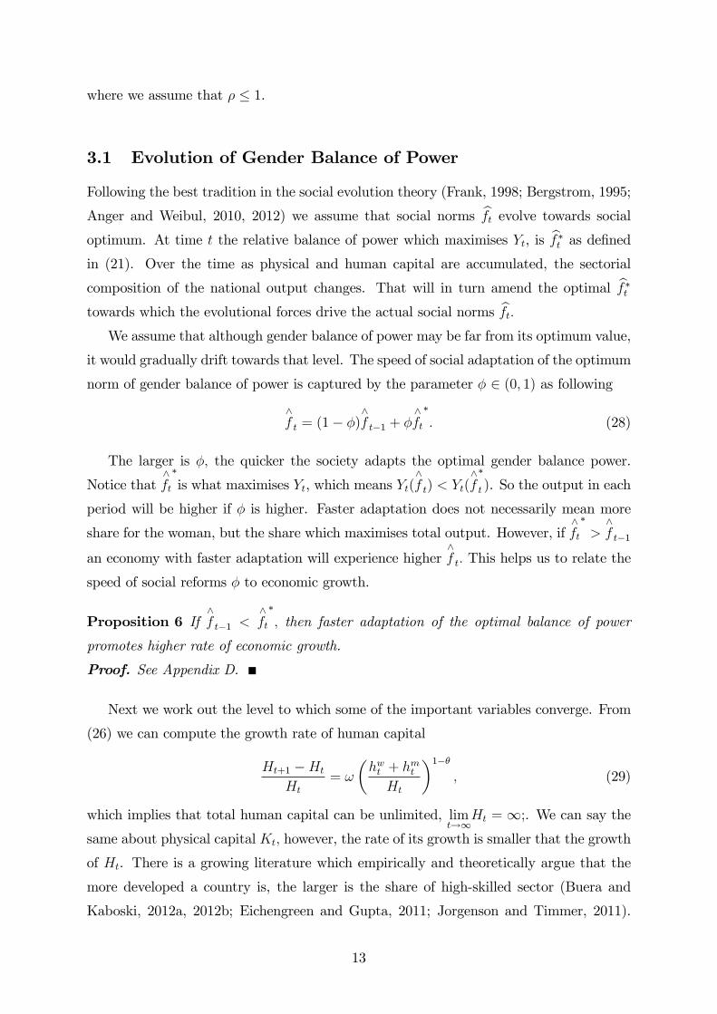
3.2.1 Relative Effort

As physical capital and human capital increases over time, woman’s relative productivity

increases, resulting in her willingness to choose higher level of effort. Moreover, the

model predicts that relative effort e would be lower in countries which starts with larger

endowment of natural resources, as shown in Figure 4,. Because the woman’s relative

14

productivity in the natural resource sector is lower than that of the man’s, her relative

effort is lower in countries with higher natural resources. Even without including religious

and cultural barriers which exist in some countries, this model explains why labour

participation rates of women is lower in countries with high natural resources.

Figure 4. Evolution of Relative Effort

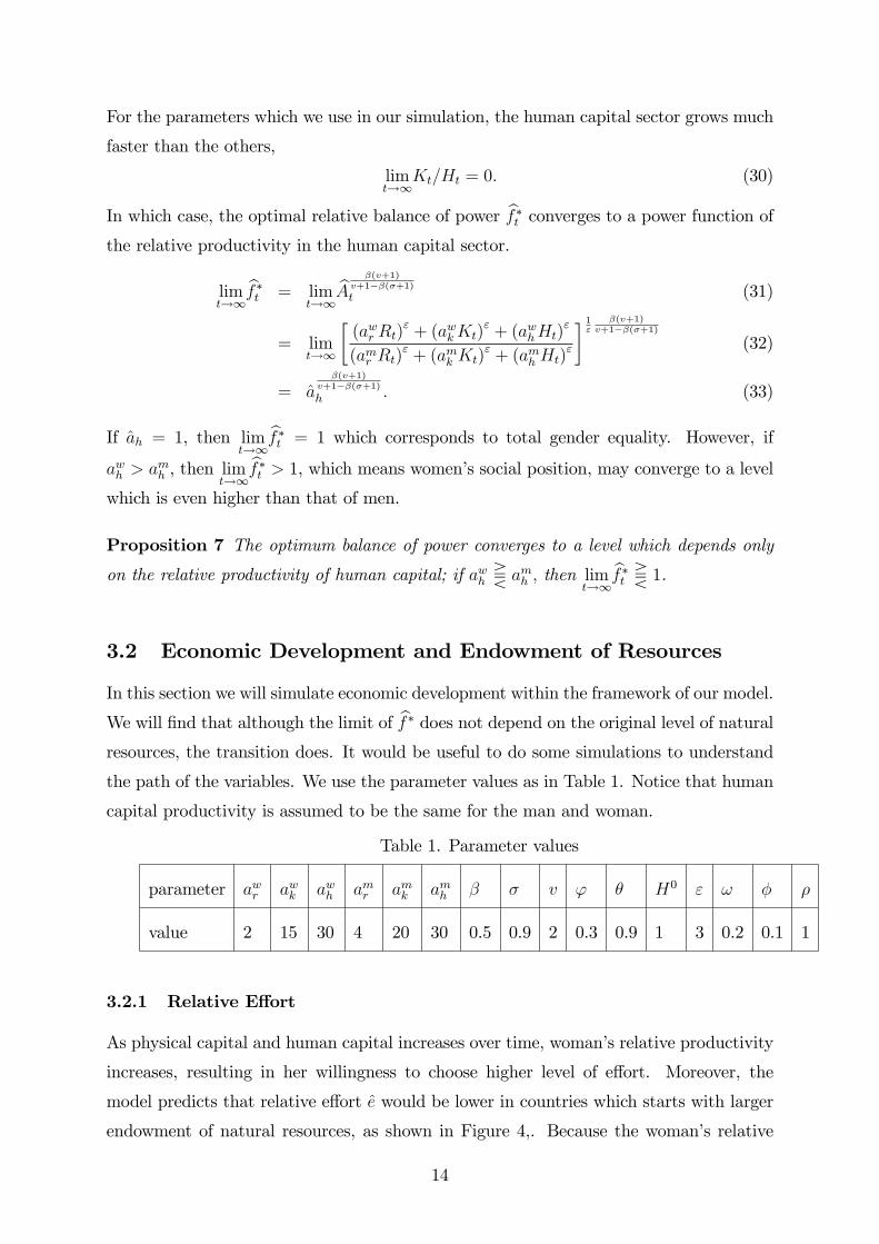
3.2.2 Human Capital

Figure 5 shows that in a country with higher natural resources, human capital is

accumulated at a lower speed by both man and woman.This is quite intuitive because

the comparative advantage in natural resources extraction demotivates the society from

investment in human capital intensive industries.

Figure 5. Evolution of investment in Human Capital

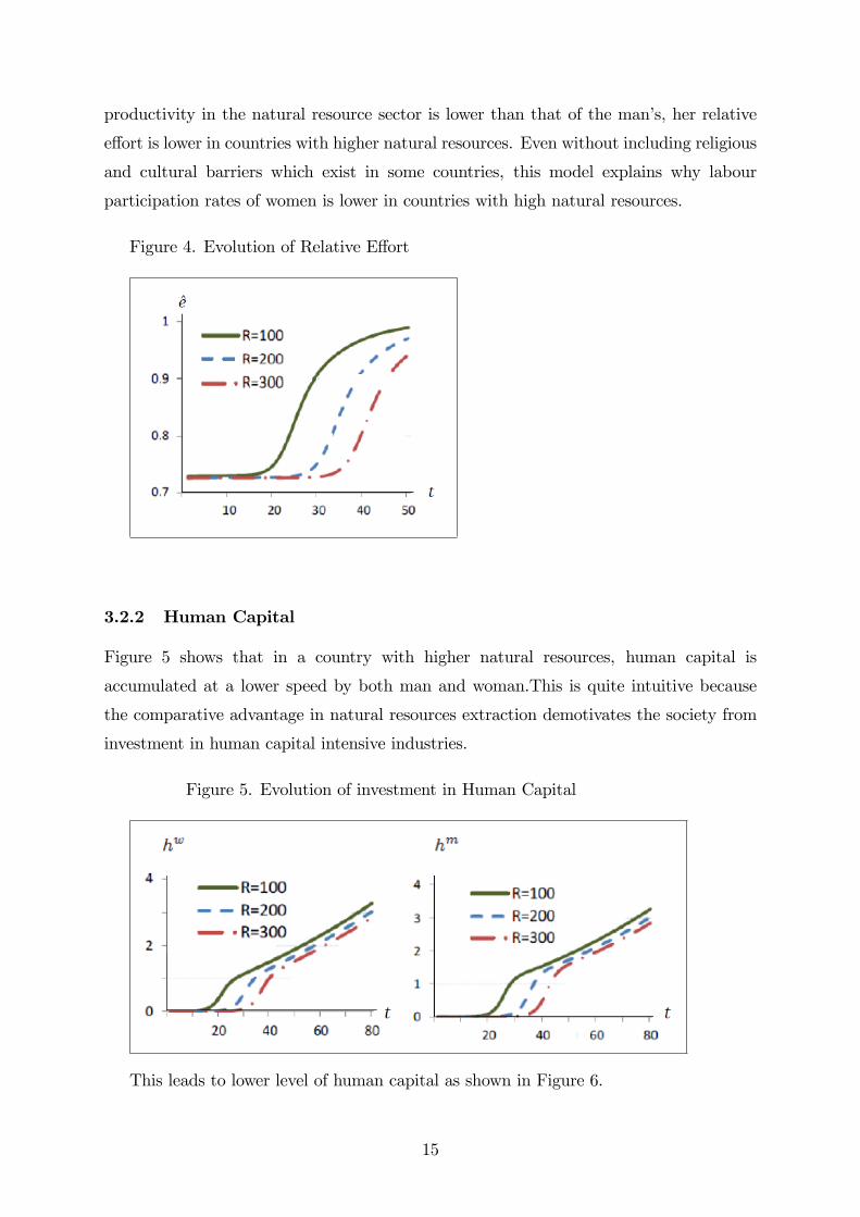
This leads to lower level of human capital as shown in Figure 6.

15

Figure 6. Evolution of Human Capital.

Although, natural resources reduce the investment into human capital by both men

and women, the model predicts, that relative contribution of effort into education by

women h would be higher in resource abundant countries, as shown in Figure 7.

Figure 7. Relative investment in Human Capital.

This is because men would choose to divert more effort into the natural resource sector

where male productivity is higher. As time goes on, the investment into education by

both men and women converge, which is shown by h reducing towards equality.

3.2.3 Production

Agents in an economy with larger level of natural resources spend a larger proportion

of effort on resource extraction and less time on education. Such an economy starts

off with higher income because it takes time for human capital accumulation. Agents

in an economy which is not endowed with much natural resources would devote more

16

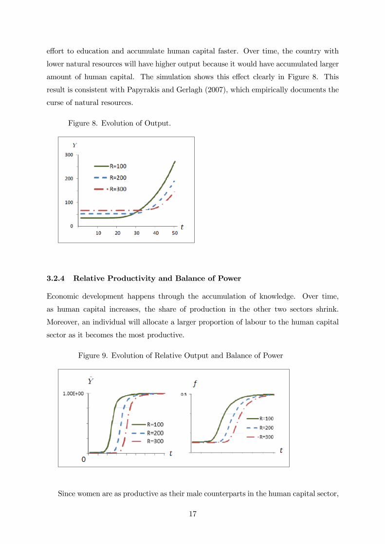
effort to education and accumulate human capital faster. Over time, the country with

lower natural resources will have higher output because it would have accumulated larger

amount of human capital. The simulation shows this effect clearly in Figure 8. This

result is consistent with Papyrakis and Gerlagh (2007), which empirically documents the

curse of natural resources.

Figure 8. Evolution of Output.

3.2.4 Relative Productivity and Balance of Power

Economic development happens through the accumulation of knowledge. Over time,

as human capital increases, the share of production in the other two sectors shrink.

Moreover, an individual will allocate a larger proportion of labour to the human capital

sector as it becomes the most productive.

Figure 9. Evolution of Relative Output and Balance of Power

Since women are as productive as their male counterparts in the human capital sector,

17

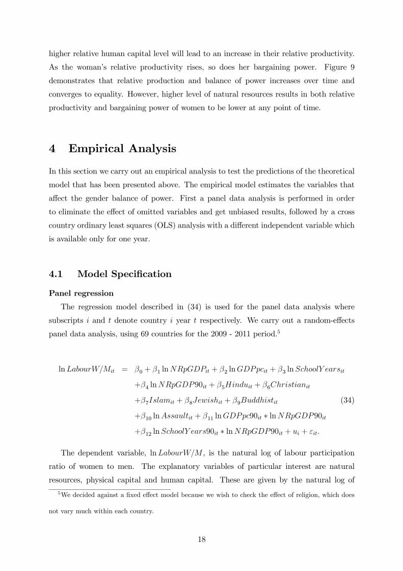
higher relative human capital level will lead to an increase in their relative productivity.

As the woman’s relative productivity rises, so does her bargaining power. Figure 9

demonstrates that relative production and balance of power increases over time and

converges to equality. However, higher level of natural resources results in both relative

productivity and bargaining power of women to be lower at any point of time.

4 Empirical Analysis

In this section we carry out an empirical analysis to test the predictions of the theoretical

model that has been presented above. The empirical model estimates the variables that

affect the gender balance of power. First a panel data analysis is performed in order

to eliminate the effect of omitted variables and get unbiased results, followed by a cross

country ordinary least squares (OLS) analysis with a different independent variable which

is available only for one year.

4.1 Model Specification

Panel regression

The regression model described in (34) is used for the panel data analysis where

subscripts i and t denote country i year t respectively. We carry out a random-effects

panel data analysis, using 69 countries for the 2009 - 2011 period.5

lnLabourW/Mit = β0 + β1 lnNRpGDPit + β2 lnGDPpcit + β3 lnSchoolY earsit

+β4 lnNRpGDP90it + β5Hinduit + β6Christianit

+β7Islamit + β8Jewishit + β9Buddhistit (34)

+β10 lnAssaultit + β11 lnGDPpc90it ∗ lnNRpGDP90it

+β12 lnSchoolY ears90it ∗ lnNRpGDP90it + ui + εit.

The dependent variable, lnLabourW/M , is the natural log of labour participation

ratio of women to men. The explanatory variables of particular interest are natural

resources, physical capital and human capital. These are given by the natural log of

5We decided against a fixed effect model because we wish to check the effect of religion, which does

not vary much within each country.

18

the rent from total natural resources (coal, forest, mineral, natural gas, oil rent) as a

percentage of GDP; the natural log of GDP per capita (constant 2005, $) and the natural

log of the average years of schooling of those over 15 years old which are denoted by

lnNRpGDP, lnGDPpc and lnSchoolY ears respectively. The effect of natural resources

on female bargaining power in the long term is captured by the natural log of natural

resources in 1990 denoted by lnNRpGDP90.6

The proxy for social norms of the previous period,∧f t−1, can be measured in terms of

safety and female-friendly environment. To capture this, we use data on the percentage

of the population following different religions in each country in 2010, Hindu, Islam,

Christian, Buddhist and Noreligion, along with the natural log of assault rate denoted

by lnAssault in 2009, which is the number of attacks per 100,000 people who suffer

physical attack against the body of another person resulting in serious bodily injury.7

The last two variables are interactive terms which show the effect of natural resources in

1990 being further enhanced by the GDP per capita and the level of education in 1990

denoted by lnGDPpc90 and lnSchoolY ears90 respectively. The summary statistics of

the variables are presented in Appendix E.

Data on labour participation ratio, account holding ratio, GDP per capita, natural

resources and school years were obtained from the world bank database. Data on religion

for 2010 is from The World Fact Book and International Religious Freedom Report for

2012. Data on assault rate is from the United Nations offi ce on drugs and crime (UNODC)

Ordinary Least Squares Regression Analysis

An ordinary least squares analysis is carried out using the model shown in (35) across

205 countries in the year 2011.

lnAccW/Mi = β0 + β1 lnNRpGDPi + β2 lnGDPpci + β3 lnSchoolY earsi

+β4 lnNRpGDP90i + β5Hindui + β6Christiani

+β7Islami + β8Jewishi + β9Buddhisti + β10 lnAssaulti (35)

+β11 lnLabourW/Mi + β12 lnSchoolY ears90i ∗ lnNRpGDP90i

+β13 lnGDPpc90i ∗ lnNRpGDP90i + ui.

The independent variable is the natural log of the ratio of women to men over 15 years

6It is diffi cult to get formal data about the level of natural resources going back many years, but 1990

will shed some light about the direction in which it affects gender balance of power.7This excludes indecent/sexual assault; threats and slapping/punching. Most of the data is for 2009

but for some countries we had to use 2008 figures because of data availability

19

old who are account holders in a formal financial institution, denoted by lnAccW/Mi.

We include the labour participation ratio lnLabourW/Mi as an explanatory variable in

this model. This is to control for outside jobs playing a role in account holding, as well

as a proxy to capture the accessibility of labour opportunities. All the other variables

are as described before.

4.2 Results and Discussion

The results of the random effect panel regression is presented in Table 2, which shows the

effect each of the explanatory variable has on lnLabourW/Mi. The results of the ordinary

least squares regression across the countries is presented in Table 3, which shows the

effect of the explanatory variables on lnAccW/Mi. Recall that female balance of power is

proxied by female labour participation ratio and the proportion of women holding bank

accounts in the panel regression and OLS regression respectively.

To avoid the problem of heteroscedasticity we use robust standard errors to determine

the significance of the variables. The robust standard errors which are shown within

parenthesis while *, ** and *** indicate the level of significance to be 10%, 5% and 1%

respectively. The results of the random effects are unbiased which eliminate ui so that

correlation between the error terms due to omitted variables that are particular to each

country is not present.

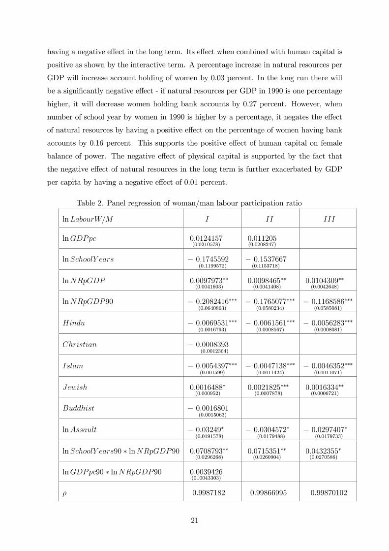
The results of the panel regression show that while the current level of natural

resources has a positive effect on female balance of power (at 5% significance level),

in the long term natural resources has a highly significant negative effect (at 1% level).

Its effect when combined with human capital is positive as shown by the interactive term

(at 10% significance level). We have also checked the effect of GDP per capita in 1990

and found it to be not significant.

A percentage increase in natural resources per GDP will increase labour participation

ratio by 0.01 percent. Natural resources being detrimental to woman’s balance of power

in the long run is supported with high significance at 1% level -if natural resources per

GDP in 1990 is one percentage higher, it will decrease female labour participation by

0.11 percent. However, when number of school years by women in 1990 is higher by a

percentage, it negates the effect of natural resources by having a positive effect on female

labour participation by 0.04 percent.

Similarly the OLS results confirm at 1% significance level that the level of natural

resources has a positive effect on female balance of power in the current period, while

20

having a negative effect in the long term. Its effect when combined with human capital is

positive as shown by the interactive term. A percentage increase in natural resources per

GDP will increase account holding of women by 0.03 percent. In the long run there will

be a significantly negative effect - if natural resources per GDP in 1990 is one percentage

higher, it will decrease women holding bank accounts by 0.27 percent. However, when

number of school year by women in 1990 is higher by a percentage, it negates the effect

of natural resources by having a positive effect on the percentage of women having bank

accounts by 0.16 percent. This supports the positive effect of human capital on female

balance of power. The negative effect of physical capital is supported by the fact that

the negative effect of natural resources in the long term is further exacerbated by GDP

per capita by having a negative effect of 0.01 percent.

Table 2. Panel regression of woman/man labour participation ratio

lnLabourW/M I II III

lnGDPpc 0.0124157(0.0210578)

0.011205(0.0208247)

lnSchoolY ears − 0.1745592(0.1199572)

− 0.1537667(0.1153718)

lnNRpGDP 0.0097973∗∗(0.0041603)

0.0098465∗∗(0.0041408)

0.0104309∗∗(0.0042648)

lnNRpGDP90 − 0.2082416∗∗∗(0.0640863)

− 0.1765077∗∗∗(0.0580234)

− 0.1168586∗∗∗(0.0585081)

Hindu − 0.0069531∗∗∗(0.0016793)

− 0.0061561∗∗∗(0.0008567)

− 0.0056283∗∗∗(0.0008081)

Christian − 0.0008393(0.0012364)

Islam − 0.0054397∗∗∗(0.001599)

− 0.0047138∗∗∗(0.0011424)

− 0.0046352∗∗∗(0.0011071)

Jewish 0.0016488∗(0.000952)

0.0021825∗∗∗(0.0007878)

0.0016334∗∗(0.0006721)

Buddhist − 0.0016801(0.0015063)

lnAssault − 0.03249∗(0.0191578)

− 0.0304572∗(0.0179488)

− 0.0297407∗(0.0179733)

lnSchoolY ears90 ∗ lnNRpGDP90 0.0708793∗∗(0.0296268)

0.0715351∗∗(0.0260904)

0.0432355∗(0.0270586)

lnGDPpc90 ∗ lnNRpGDP90 0.0039426(0..0043303)

ρ 0.9987182 0.99866995 0.99870102

21

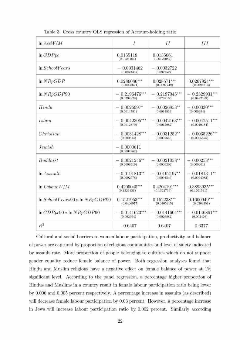
Table 3. Cross country OLS regression of Account-holding ratio

lnAccW/M I II III

lnGDPpc 0.0155119(0.0125184)

0.0155661(0.0126082)

lnSchoolY ears − 0.0031462(0.0973487)

− 0.0032722(0.0972527)

lnNRpGDP 0.0286086∗∗∗(0.0098621)

0.028571∗∗∗(0.0097749)

0.0267924∗∗∗(0.0096213)

lnNRpGDP90 − 0.2196476(0.0794928)

∗∗∗ − 0.2197045(0.0792166)

∗∗∗ − 0.2329931(0.0482189)

∗∗∗

Hindu − 0.0026997(0.0014781)

∗ − 0.0026853(0.0014833)

∗∗ − 0.00330(0.000994)

∗∗∗

Islam − 0.0042305(0.0012879)

∗∗∗ − 0.0042163(0.0012982)

∗∗∗ − 0.0047511(0.0010184)

∗∗∗

Christian − 0.0031428(0.000814)

∗∗∗ − 0.0031252(0.0007646)

∗∗ − 0.0035226(0.0005525)

∗∗∗

Jewish − 0.0000611(0.0004962)

Buddhist − 0.0021246(0.0009519)

∗∗ − 0.0021058(0.0009206)

∗∗ − 0.00253(0.000601)

∗∗∗

lnAssault − 0.0191813(0.0092578)

∗∗ − 0.0192197(0.0091546)

∗∗ − 0.0181311(0.0094082)

∗∗

lnLabourW/M 0.4205045(0.1329131)

∗∗∗ 0.4204191(0.1322736)

∗∗∗ 0.3893935(0.1201541)

∗∗∗

lnSchoolY ears90 ∗ lnNRpGDP90 0.1521953∗∗∗(0.0406977)

0.152238∗∗∗(0.0405315)

0.1600949∗∗∗(0.0264151)

lnGDPpc90 ∗ lnNRpGDP90 − 0.0141623(0.002694)

∗∗∗ − 0.0141604(0.0026882)

∗∗∗ − 0.0146861(0.002426)

∗∗∗

R2 0.6407 0.6407 0.6377

Cultural and social barriers to women labour participation, productivity and balance

of power are captured by proportion of religious communities and level of safety indicated

by assault rate. More proportion of people belonging to cultures which do not support

gender equality reduce female balance of power. Both regression analyses found that

Hindu and Muslim religions have a negative effect on female balance of power at 1%

significant level. According to the panel regression, a percentage higher proportion of

Hindus and Muslims in a country result in female labour participation ratio being lower

by 0.006 and 0.005 percent respectively. A percentage increase in assaults (as described)

will decrease female labour participation by 0.03 percent. However, a percentage increase

in Jews will increase labour participation ratio by 0.002 percent. Similarly according

22

to the OLS analysis, a percentage higher proportion of Hindus, Muslims, Christians

and Buddhists in a country result in the percentage of women holding bank account

being lower by 0.003, 0.005, 0.003 and 0.003 percent respectively. A percentage increase

in assaults will decrease percentage of women holding bank accounts by 0.02 percent.

A percentage increase in women to men labour participation ratio will result in the

percentage of women holding financial account by 0.39 percentage which is statistically

highly significant at 1% level.

5 Conclusion

This paper explains the difference in gender balance of power across countries and

across time. We based our model on the assumption that social norms evolve towards

those maximising economic production. We show that an increase in woman’s relative

productivity will increase her bargaining power. The dynamic framework highlights

the negative impact of natural resources and positive impact of human capital on the

evolution of female balance of power. The empirical analysis with recent data supports

this prediction. The dynamic model predicts that the gender balance of power converges

to equality only when women are as productive as men in human capital intensive

industries.

References

[1] Alfano., W. Arulampalam., and U. Kambhampati (2011). "Maternal Autonomy and

the Education of the Subsequent Generation: Evidence from three Contrasting States

in India". IZA Discussion Papers 6019.

[2] Alger, I., and J. W. Weibull, (2010). "Kinship, Incentives, and Evolution," American

Economic Review, American Economic Association, vol. 100(4), pages 1725-58,

September.

[3] Alger, I., and J. W. Weibull (2013). "Homo Moralis– Preference Evolution Under

Incomplete Information and Assortative Matching," Econometrica, Vol. 81(6), pp

2269-2302.

23

[4] Allen, S, G. (2001). "Technology and the Wage structure", Journal of Labour

Economics, Vol. 19.2 pp 440 —482.

[5] Almond., L. Edlund., and K. Milligan (2009). "O Sister, Where Art Thou? The Role

of Son Preference and Sex Choice: Evidence from Immigrants to Canada". NBER

Working Paper 15391.

[6] Arulampalam, W., A. L. Booth., and M. L. Bryan (2007). "Is there a Glass Ceiling

Over Europe? Exploring the Gender Pay Gap Across the Wage Distribution".

Industrial and Labour Relations Review Vol. 60 (2) pp 163 - 186.

[7] Barro, R. J. and J. W. Lee (1994). "Sources of Economic Growth". Carnegie-

Rochester Conference Series on Public Policy, Volume 40, pp 1—46.

[8] Becker, G. S., K. M. Murphy and R. Tamura (1990). "Human Capital, Fertility,

and Economic Growth", Journal of Political Economy, Vol. 98, No. 5, Part 2,

The Problem of Development: A Conference of the Institute for the Study of Free

Enterprise Systems (Oct., 1990), pp. S12-S37.

[9] Bergstrom, T. C. (1995), "On the Evolution of Altruistic Ethical Rules for Siblings,"

American Economic Review, American Economic Association, Vol. 85(1), pp 58-81.

[10] Bhaskar, V., and B. Gupta (2007). "India’s Missing Girls: Biology, Customs and

Economic Development". Oxford Review of Economic Policy Vol. 2 No. 2, pp 221 -

238.

[11] Blau, F.D. (1998). "Trends in the Well-Being of American Women, 1970-1995".

Journal of Economic Literature XXXVI(1), 112-165.

[12] Borooah, V. and Mangan, J. (2009). "Home is where the hurt is: a statistical analysis

of injuries caused by spousal assault". Applied Economics, Vol. 41, Issue 21, pp 2779

- 2787.

[13] Buchmann, C., and T. A. DiPrete (2006). "The Growing Female Advantage in

College Completion: The Role of Family Background and Academic Achievement"

American Sociological Review, Vol. 71, No. 4. pp. 515-541.

[14] Buera, F. J., and J. P. Kaboski. (2012a). "The Rise of the Service Economy".

American Economic Review, 102(6), 2540 - 2569.

24

[15] Buera, F. J., and J. P. Kaboski. (2012b). "Scale and the Organiser Structured

Change". Journal of Economic Theory, 142.2, 684 - 712.

[16] Card, D and J. E. DiNardo (2002). "Skill-biased technological change and rising

wage inequality: some problems and puzzles" Journal of Labour Economics, Vol. 20,

No 4, pp 733 - 783.

[17] Charles, K and M. C. Luoh, (2003). "Gender differences in completed schooling",

Review of Economics and Statistics, 85(3), pp 559 - 77.

[18] Deolalikar, A. B. (1993). "Gender differences in the returns to schooling and in school

enrollment rates in Indonesia". The Journal of Human Resources, pp 899 - 932.

[19] Dollar, D and R. Gatti (1999). "Gender Inequality, Income, and Growth: Are Good

Times Good for Women?". Policy Research Report on Gender and Development,

The World Bank Working Paper Series, No. 1.

[20] Dugan, L., Nagin, D. and Rosenfeld, R. (1998). "Explaining the decline in intimate

partner homicide: the effect of changing domesticity, women’s status and domestic

violence resources". Homicide Studies, 3(3).

[21] Edin, Per-Anders and Katarina Richardson, 2002, Swimming with the Tide: Solidary

Wage Policy and the Gender Earnings Gap, The Scandinavian Journal of Economics,

Vol. 104, No. 1 (Mar., 2002), pp. 49-67

[22] Edlund, L., and C. Lee (2013). "Son Preference, Sex Selection and Economic

Development: The Case of South Korea". NBER Working Papers 18679.

[23] Eichengreen, B., and P. Gupta (2011). "The two-waves of service sector growth".

Oxford Economic Papers 65(1) 96 - 123.

[24] Farmer, A. and Tiefenthaler, J. (2003). "Explaining the Recent Decline in Domestic

Violence". Contemporary Economic Policy, 21(2), 158-172.

[25] Frank, S. A. (1998). Foundations of Social Evolution. Princeton, N. J.: Princeton

University Press.

[26] Goldin, Claudia. 2006. “The Quiet Revolution That Transformed Women’s Employ-

ment, Education, and Family.”A.E.R. Papers and Proc. 96 (May): 1—21

25

[27] Heathcote Jonathan , Kjetil Storesletten and Giovanni L. Violante, The Macro-

economic Implications of Rising Wage Inequality in the United States,Journal of

Political Economy, Vol. 118, No. 4 (August 2010), pp. 681-722

[28] Hamilton, W. D. (1964). “Genetical Evolution of Social Behavior I and II”Journal

of Theoretical Biology 7: 1-52.

[29] Heckman , J. J. and T. E. Macurdy, (1980). "A Life Cycle Model of Female Labour

Supply", The Review of Economic Studies , Vol. 47, No. 1, Econometrics Issue, pp.

47-74.

[30] Hill, M. A and E. King (1995). "Women’s education and economic well-being".

Feminist Economics Volume 1, Issue 2, pp 21 - 46.

[31] Iyigun, M. F. and R. P. Walsh (2007), "Endogenous gender power, household labour

supply and the quantity - quality trade-off". Journal of Development Economics, 138

- 155.

[32] Jorgenson, D. W., and M. O. Timmer. (2011). "Structural change in Advanced

Nations: A New Set of Stylised Facts". Scandinavian Journal of Economics 113 (1),

1 - 29.

[33] Klasen, S. (2002). "Low Schooling for Girls, Slower Growth for All? Cross-

Country Evidence on the Effect of Gender Inequality in Education on Economic

Development". The World Bank Economic Review, Volume 16 Issue 3, pp 345 - 373.

[34] Klasen, S and F. Lamanna (2009). "The Impact of Gender Inequality in Education

and Employment on Economic Growth: New Evidence for a Panel of Countries".

Feminist Economics, Vol. 15, Issue 3, pp 91 - 132.

[35] Knowles, S., P. K. Lorgelly and P. D. Owen (2002). "Are educational gender gaps

a brake on economic development? Some cross-country empirical evidence". Oxford

Economic Papers, Vol. 54 Issue 1, pp 118 - 149.

[36] Kury, H., Obergfell-Fuchs, J. andWoessner, G. (2004). "The extent of family violence

in Europe, Violence Against Women". 10(7), 749-769.

[37] Levin, B.R., and W. L. Kilmer (1974). "Interdemic selection and the evolution of

altruism: a computer simulation study". Evolution 28, pp 527—545.

26

[38] Lundberg, S and R. A. Pollak (2003). "Effi ciency in Marriage". Review of Economics

of the Household, pp 153 - 167.

[39] Machin, S and S. McNally, (2005). "Gender and student achievement in English

schools". Oxford Review of Economic Policy, Vol. 21. 3, pp 357 - 372.

[40] Max, W., Rice, D.P., Finkelstein, E., Bardwell R. A. and Leadbetter, S. (2004).

"The economic toll of intimate partner violence against women in the United States".

Violence and Victims, 19(3), 259-72.

[41] Mulligan Casey B. and Yona Rubinstein,(2008), "Selection, Investment, and

Women’s Relative Wages over Time,", The Quarterly Journal of Economics, Vol.

123, No. 3, pp. 1061-1110

[42] Olivetti, C., Petrongolo, B. (2011). "Gender gaps across countries and skills: supply,

demand and the industry structure". Review of Economic Dynamics Vol. 17, Issue

4, pp 842 - 859.

[43] Papyrakis, E., & Gerlagh, R. (2007). "Resource abundance and economic growth in

the United States". European Economic Review, 51(4), pp 1011-103

[44] Psacharopoulos, G. (1994) "Returns to investment in education: A global update".

World Development, Volume 22, Issue 9, Pages 1325—1343.

[45] Rainer, H. (2008). "Gender discrimination and effi ciency in marriage: the bargaining

family under scrutiny". Journal of Population Economics 21, pp 305 - 329.

[46] Schultz, T. P. (1995). "Woman’s human capital". University of Chicago Press.

[47] Schultz, T. P. (2002). "Why Governments Should Invest More to Educate Girls".

World Development, Volume 30, Issue 2, Pages 207—225.

[48] Solow, Robert M. (1956). "A contribution to the theory of economic growth".

Quarterly Journal of Economics (Oxford Journals) 70 (1): 65—94.

27

6 Appendix

A. Proof of Proposition 1

The woman’s share f is chosen to maximise Y , subject to the two effort supply

equation

LY = (Y m + Y w) + sw (fwuwc Ywe − V w

e ) + sm ((1− fw)umc Y me − V m

e ) . (A1)

The first order conditions are presented below

dLY

dfw= sw (uwc Y

we + fwY uwccY

we )− smfmY umccY m

e − smumc Y me = 0

dLY

dew= Y w

e + sw[(fw)2 uwccY

we Y

we + fwuwc Y

wee − V w

ee

]+ sm(fm)2umccY

me Y

we = 0 (A2)

dLY

dem= Y m

e + sw((fw)2 uwccY

we Y

me

)+ sm

[(fm)2umccY

me Y

me + fm)umc Y

mee − V m

ee

]= 0.

We solve the system using the functional forms uj = (Cj)σ

σ, V j = κ (e

j)1+v

1+v. First we define

elasticity ηjuc,c =fjY ujccujc

; ηjVe,e =Veeej

Ve; ηjYe,e =

Y jeeej

Y je; ηjY,e =

Y je ej

Y j. We use that definition in

the above equations to get

dLY

dfw= swuwc Y

wew

(1 + ηwuc,c

)− smumc Y me

(1 + ηmuc,c

)= 0

dLY

dew= Y we + smfm

(ηmuc,cu

mc

Y me Y weY

)+ sw

[fwηwuc,c

uwcYY we Y

we + fwuwc

Y weew

ηwYe,e − ηwVe,e

V weew

]= 0(A3)

dLY

dem= Y me + sm

[fmηmuc,cu

mc

Y me Y meY

+ fmumcY meem

ηmYe,e − ηmVe,e

V meem

]+ sw

(fwηwuc,cu

wc

Y we Yme

Y

)= 0.

We can rewrite this using effort supply equation (7), f jujcYje = V j

e

dLY

dfw= swuwc Y

we

(1 + ηwuc,c

)− smumc Y me

(1 + ηmuc,c

)= 0;

dLY

dew= Y we + smfmumc Y

me ηmuc,c

Y weY+ swuwc

Y weew

fw[ηwuc,c

Y we ew

Y+ ηwYe,e − η

wVe,e

]= 0; (A4)

dLY

dem= Y me + smfmumc

Y meem

[ηmuc,c

Y meYem + ηmYe,e − η

mVe,e

]+ swuwc Y

wew

(fwηwuc,c

Y meY

)0.

28

We substitute for one of the Lagrange multiplier, smumc Ymem = swuwc Y

wew(1+ηwuc,c)(1+ηmuc,c)

dLY

dew= Y wew + s

wuwc Ywe

1 + ηwuc,c

1 + ηmuc,cfmηmuc,c

Y weY+ swuwc Y

wew1

ewfw[ηwuc,c

Y we ew

Y+ ηwYe,e − η

wVe,e

]= 0,(A5)

dLY

dem= Y mem + s

wuwc Ywe

1 + ηwuc,c

1 + ηmuc,cfm

1

em

[1

Yηmuc,cY

me em + ηmYe,e − η

mVe,e

]+ swuwc Y

we f

wηwuc,cY meY

= 0.

(A6)

and combine that in one relation as

Y we e

w

Y me e

m=

(1 + ηwuc,c

)fmηmuc,c

Y we ew

Y+(1 + ηmuc,c

)fw[ηwuc,c

Y we ew

Y+ ηwYe,e − ηwVe,e

](1 + ηwuc,c

)fm[Yme em

Yηmuc,c + ηmYe,e − ηmVe,e

]+(1 + ηmuc,c

)fwηwuc,c

Yme em

Y

, (A7)

we simplify it further using elasticities

ηwY,eYw

ηmY,eYm=

(1 + ηwuc,c

)fmηmuc,cη

wY,eY

w +(1 + ηmuc,c

)fw[ηwuc,cη

wY,eY

w +(ηwYe,e − ηwVe,e

)Y]

(1 + ηwuc,c

)fm[ηmY,eY

mηmuc,c +(ηmYe,e − ηmVe,e

)Y]+ fwηwuc,c

(1 + ηmuc,c

)Y mηmuc,c

.

(A8)

In our simple case when all functions have constant elasticities and the functional forms

are the same for man and woman, it can be simplified as Y w

Ym= fw

fm.

B. Proof of Proposition 3

The Lagrangian of the decision problem when choosing ew and its allocation to the

three sectors optimally by j = w is solved below.

L =

[f((Awew)β + Y M)

]σσ

− (ew)v+1

v + 1

−µ[Awew −

((awr Rr

w)εε+1 + (awl Kl

w)εε+1 + (awhHh

w)εε+1

) ε+1ε

](B1)

−λ (−ew + [rw + lw + hw]) ,

The first order conditions are

∂L

∂AwAw = fβ (Awew)β

[f((Awew)β + Y M)

]σ−1− µewAw = 0;

∂L

∂ewew = fβ (Awew)β

[f((Awew)β + Y M)

]σ−1− µAwew − (ew)v+1 + λew = 0;

∂L

∂rwrw = µ (Awew)

1ε+1 (awr Rr

w)εε+1 − λrw = 0; (B3)

∂L

∂lwlw = µ (Awew)

1ε+1 (awl Kl

w)εε+1 − λlw = 0;

∂L

∂hwhw = µ (Awew)

1ε+1 (awhHh

w)εε+1 − λhw = 0.

29

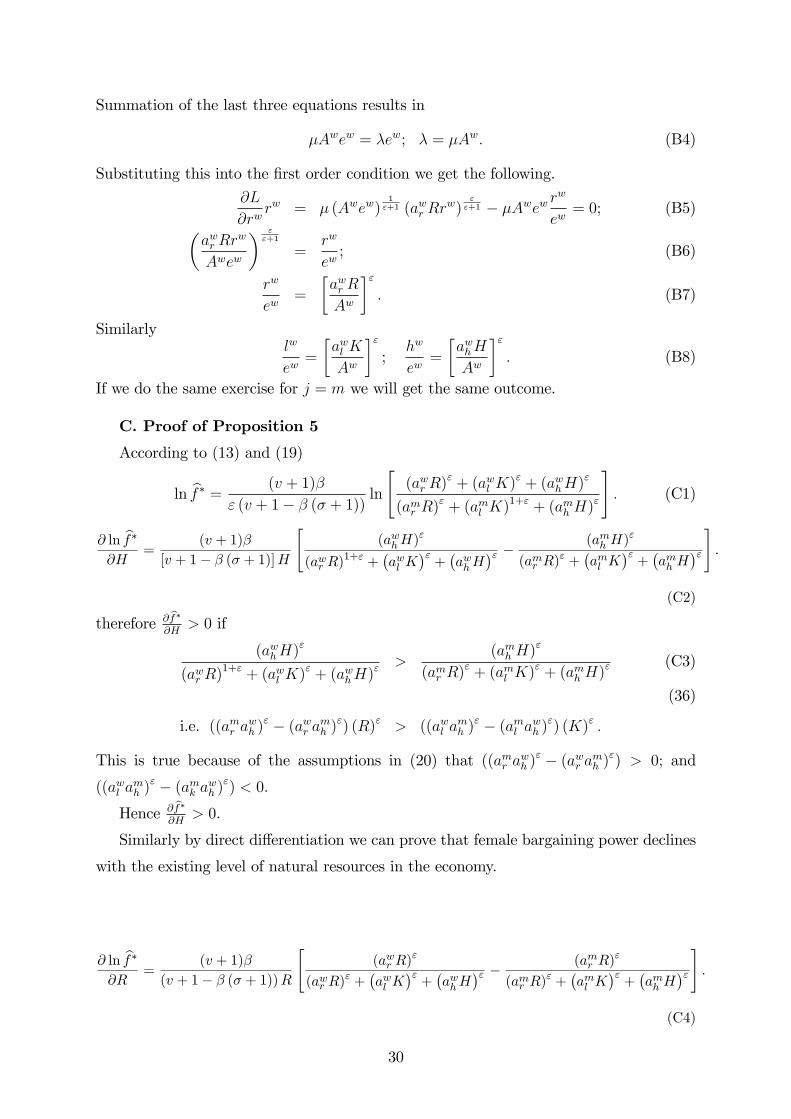
Summation of the last three equations results in

µAwew = λew; λ = µAw. (B4)

Substituting this into the first order condition we get the following.

∂L

∂rwrw = µ (Awew)

1ε+1 (awr Rr

w)εε+1 − µAwew r

w

ew= 0; (B5)(

awr Rrw

Awew

) εε+1

=rw

ew; (B6)

rw

ew=

[awr R

Aw

]ε. (B7)

Similarlylw

ew=

[awl K

Aw

]ε;

hw

ew=

[awhH

Aw

]ε. (B8)

If we do the same exercise for j = m we will get the same outcome.

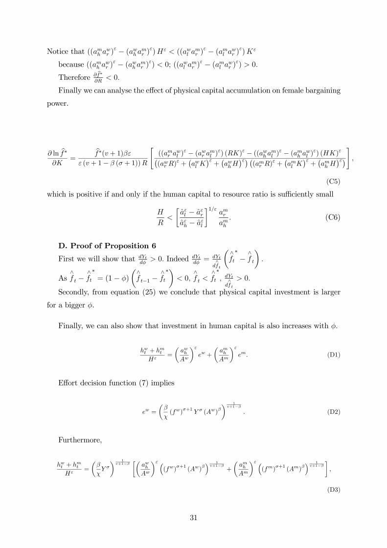
C. Proof of Proposition 5

According to (13) and (19)

ln f ∗ =(v + 1)β

ε (v + 1− β (σ + 1)) ln[(awr R)

ε + (awl K)ε + (awhH)

ε

(amr R)ε + (aml K)

1+ε + (amh H)ε

]. (C1)

∂ ln f∗

∂H=

(v + 1)β

[v + 1− β (σ + 1)]H

[(awhH)

ε

(awr R)1+ε +

(awl K

)ε+(awhH

)ε − (amh H)ε

(amr R)ε +

(aml K

)ε+(amh H

)ε].

(C2)

therefore ∂f∗

∂H> 0 if

(awhH)ε

(awr R)1+ε + (awl K)

ε + (awhH)ε >

(amh H)ε

(amr R)ε + (aml K)

ε + (amh H)ε (C3)

(36)

i.e. ((amr awh )

ε − (awr amh )ε) (R)ε > ((awl a

mh )

ε − (aml awh )ε) (K)ε .

This is true because of the assumptions in (20) that ((amr awh )

ε − (awr amh )ε) > 0; and

((awl amh )

ε − (amk awh )ε) < 0.

Hence ∂f∗

∂H> 0.

Similarly by direct differentiation we can prove that female bargaining power declines

with the existing level of natural resources in the economy.

∂ ln f∗

∂R=

(v + 1)β

(v + 1− β (σ + 1))R

[(awr R)

ε

(awr R)ε +

(awl K

)ε+(awhH

)ε − (amr R)ε

(amr R)ε +

(aml K

)ε+(amh H

)ε].

(C4)

30

Notice that ((amh awr )

ε − (awh amr )ε)Hε < ((awl a

mr )

ε − (aml awr )ε)Kε

because ((amh awr )

ε − (awh amr )ε) < 0; ((awl a

mr )

ε − (aml awr )ε) > 0.

Therefore ∂f∗

∂R< 0.

Finally we can analyse the effect of physical capital accumulation on female bargaining

power.

∂ ln f∗

∂K=

f∗(v + 1)βε

ε (v + 1− β (σ + 1))R

[((amr a

wl )ε − (awr aml )

ε) (RK)ε − ((awh aml )ε − (amh awl )

ε) (HK)ε((awr R)

ε +(awl K

)ε+(awhH

)ε) ((amr R)

ε +(aml K

)ε+(amh H

)ε)],

(C5)

which is positive if and only if the human capital to resource ratio is suffi ciently small

H

R<

[aεl − aεraεh − aεl

]1/εamramh

. (C6)

D. Proof of Proposition 6

First we will show that dYtdφ

> 0. Indeed dYtdφ= dYt

d∧f t

(∧ft

∗−∧f t

).

As∧f t −

∧ft

∗= (1− φ)

(∧f t−1 −

∧ft

∗)< 0,

∧f t <

∧ft

∗, dYtd∧f t

> 0.

Secondly, from equation (25) we conclude that physical capital investment is larger

for a bigger φ.

Finally, we can also show that investment in human capital is also increases with φ.

hwt + hmt

Hε=

(awhAw

)εew +

(amhAm

)εem. (D1)

Effort decision function (7) implies

ew =

(β

χ(fw)

σ+1Y σ (Aw)

β

) 1v+1−β

. (D2)

Furthermore,

hwt + hmt

Hε=

(β

χY σ) 1v+1−β

[(awhAw

)ε ((fw)

σ+1(Aw)

β) 1v+1−β

+

(amhAm

)ε ((fm)

σ+1(Am)

β) 1v+1−β

],

(D3)

31

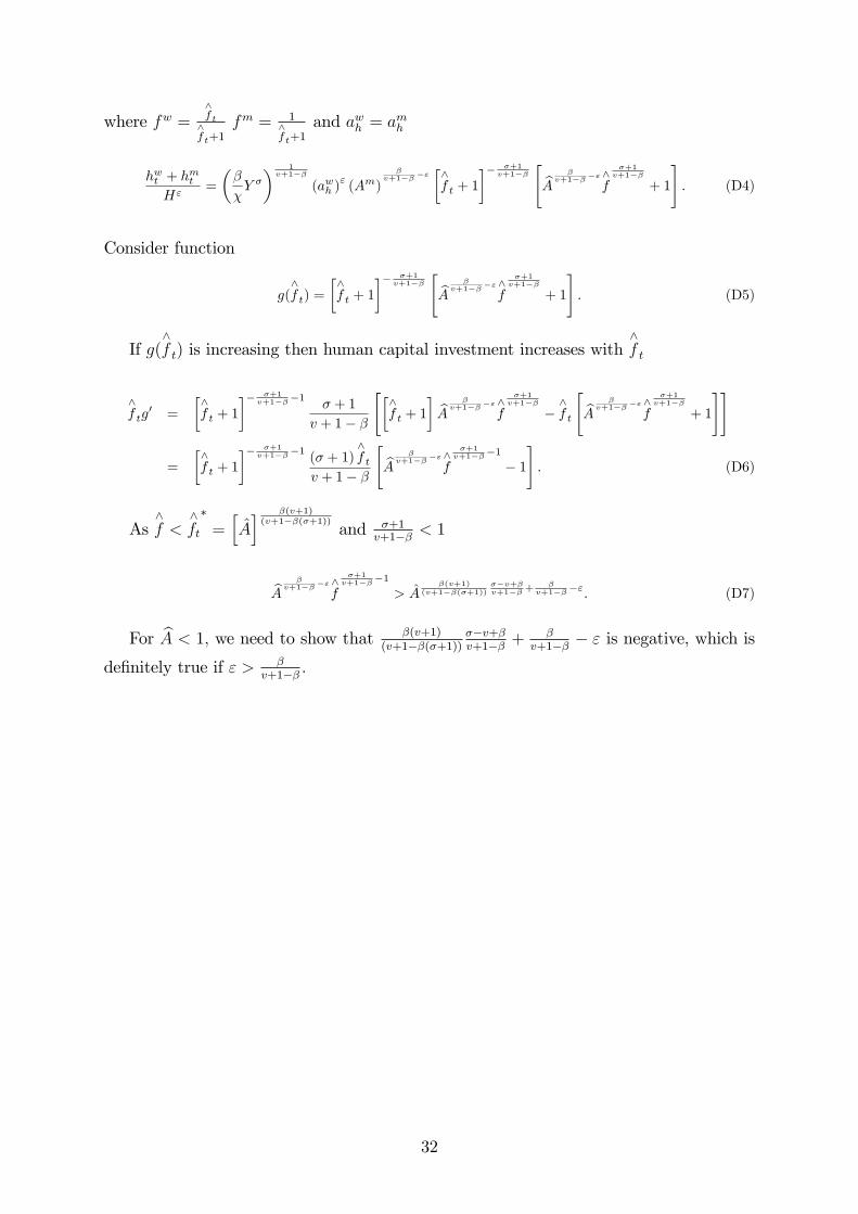
where fw =∧f t∧f t+1

fm = 1∧f t+1

and awh = amh

hwt + hmt

Hε=

(β

χY σ) 1v+1−β

(awh )ε(Am)

βv+1−β−ε

[∧f t + 1

]− σ+1v+1−β

[A

βv+1−β−ε∧

f

σ+1v+1−β

+ 1

]. (D4)

Consider function

g(∧f t) =

[∧f t + 1

]− σ+1v+1−β

[A

βv+1−β−ε∧

f

σ+1v+1−β

+ 1

]. (D5)

If g(∧f t) is increasing then human capital investment increases with

∧f t

∧f tg′ =

[∧f t + 1

]− σ+1v+1−β−1 σ + 1

v + 1− β

[[∧f t + 1

]A

βv+1−β−ε∧

f

σ+1v+1−β

−∧f t

[A

βv+1−β−ε∧

f

σ+1v+1−β

+ 1

]]

=

[∧f t + 1

]− σ+1v+1−β−1 (σ + 1)

∧f t

v + 1− β

[A

βv+1−β−ε∧

f

σ+1v+1−β−1

− 1]. (D6)

As∧f <

∧ft

∗=[A] β(v+1)(v+1−β(σ+1))

and σ+1v+1−β < 1

Aβ

v+1−β−ε∧f

σ+1v+1−β−1

> Aβ(v+1)

(v+1−β(σ+1))σ−v+βv+1−β +

βv+1−β−ε. (D7)

For A < 1, we need to show that β(v+1)(v+1−β(σ+1))

σ−v+βv+1−β +

βv+1−β − ε is negative, which is

definitely true if ε > βv+1−β .

32

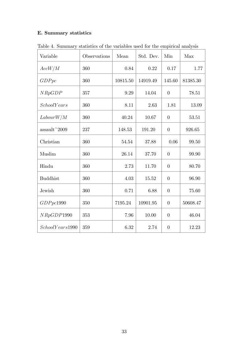
E. Summary statistics

Table 4. Summary statistics of the variables used for the empirical analysis

Variable Observations Mean Std. Dev. Min Max

AccW/M 360 0.84 0.22 0.17 1.77

GDPpc 360 10815.50 14919.49 145.60 81385.30

NRpGDP 357 9.29 14.04 0 78.51

SchoolY ears 360 8.11 2.63 1.81 13.09

LabourW/M 360 40.24 10.67 0 53.51

assault~2009 237 148.53 191.20 0 926.65

Christian 360 54.54 37.88 0.06 99.50

Muslim 360 26.14 37.70 0 99.90

Hindu 360 2.73 11.70 0 80.70

Buddhist 360 4.03 15.52 0 96.90

Jewish 360 0.71 6.88 0 75.60

GDPpc1990 350 7195.24 10901.95 0 50608.47

NRpGDP1990 353 7.96 10.00 0 46.04

SchoolY ears1990 359 6.32 2.74 0 12.23

33