Embed Size (px)
Citation preview

Economic Filters for Evaluating Porphyry Copper Deposit Resource Assessments Using Grade-Tonnage Deposit Models, with Examples from the U.S. Geological Survey Global Mineral Resource Assessment
Scientific Investigations Report 2010–5090–H
Version 1.2, March 2014
U.S. Department of the InteriorU.S. Geological Survey
Global Mineral Resource Assessment

This page left intentionally blank.

Economic Filters for Evaluating Porphyry Copper Deposit Resource Assessments Using Grade-Tonnage Deposit Models, with Examples from the U.S. Geological Survey Global Mineral Resource Assessment
By Gilpin R. Robinson, Jr., and W. David Menzie
Scientific Investigations Report 2010–5090–H
U.S. Department of the InteriorU.S. Geological Survey
Global Mineral Resource Assessment
Michael L. Zientek, Jane M. Hammarstrom, and Kathleen M. Johnson, editors
Version 1.2, March 2014

U.S. Department of the InteriorKEN SALAZAR, Secretary
U.S. Geological SurveyMarcia K. McNutt, Director
U.S. Geological Survey, Reston, Virginia: 2012
Revised: March 2014, version 1.2
For more information on the USGS—the Federal source for science about the Earth, its natural and living resources, natural hazards, and the environment—visit http://www.usgs.gov or call 1–888–ASK–USGS For an overview of USGS information products, including maps, imagery, and publications, visit http://www.usgs.gov/pubprod
Suggested citation:Robinson, G.R., Jr., and Menzie, W.D., 2012, Economic filters for evaluating porphyry copper deposit resource assessments using grade-tonnage deposit models, with examples from the U.S. Geological Survey global mineral resource assessment (ver 1.2, March 2014): U.S. Geological Survey Scientific Investigations Report 2010–5090–H, 21 p., http://pubs.usgs.gov/sir/2010/5090/h/.
Any use of trade, product, or firm names is for descriptive purposes only and does not imply endorsement by the U.S. Government. Although this information product, for the most part, is in the public domain, it also may contain copyrighted materials as noted in the text. Permission to reproduce copyrighted items must e secured from the copyright owner.

iii
ContentsAbstract ...........................................................................................................................................................1Introduction.....................................................................................................................................................1
Terminology ............................................................................................................................................2Overview of Grade and Tonnage Models and Simplified Economic Filters .........................................2
Simplified Mining Engineering Cost Models ....................................................................................4Overview of Engineering Cost Models .....................................................................................4USBM Simplified Mining Engineering Cost Models ..............................................................5
Mine Capacity and Lifetime ..............................................................................................6Mine Models ........................................................................................................................6Mill Models ..........................................................................................................................7Infrastructure Models (Tailings Pond, Dam, and Liner) ................................................7Adjustments to Cost Equations for High Cost Settings .................................................8Cost Updating ......................................................................................................................8
Summary........................................................................................................................................8Economic Filters for Porphyry Copper Deposits ..............................................................................8
Commodity Prices and Calculation of Copper Equivalent Grades ......................................9Updating the Engineering Cost Models ...................................................................................9Porphyry Copper Deposit Economic Filter Example ..............................................................9Comparison of the Economic Filters with a Recent Analysis of the
Economic Status of Copper Deposits .......................................................................10Application of Economic Filters on Six Assessment Tract Results .....................................................10
Economic Filters Applied to the Six Tract Areas ...........................................................................11Application of the Economic Filter to Estimates of Undiscovered Resources
in the Six Tracts .....................................................................................................................14Examples of Tract-Based Economic Filter Results ........................................................................17
Conclusions...................................................................................................................................................17References Cited..........................................................................................................................................19
Figures1. Cumlative copper resources in the general porphyry copper deposit grade-tonnage model
as a percentage of ranked deposits accumulated .................................................................32. Cumulative copper resources in the general porphyry
copper deposit grade-tonnage model showing deposit importance categories ..............43. Tonnage and copper grade characteristics of deposits in the general porphyry copper
deposit grade-tonnage model ....................................................................................................54. Comparison of the cutoff grade calculated for porphyry copper deposits
using updated simplified engineering cost models for open-pit and block caving mines as a function of deposit depth and ore tonnage ................................11
5. Selected permissive tracts for porphyry copper deposits in North America ............................136. Sensitivity of expected number of economic deposits and amount of copper resources
in porphyry copper deposits composing the general porphyry copper model ................14

iv
Conversion FactorsInch/Pound to SI
Multiply By To obtainLength
foot (ft) 0.3048 meter (m)mile (mi) 1.609 kilometer (km)yard (yd) 0.9144 meter (m)
Areasquare mile (mi2) 2.590 square kilometer (km2)
Masston, short (2,000 lb) 0.9072 metric ton (mt) ton per day (ton/d) 0.9072 metric ton per day
SI to Inch/Pound
Multiply By To obtainLength
meter (m) 3.281 foot (ft) kilometer (km) 0.6214 mile (mi)meter (m) 1.094 yard (yd)
Areasquare kilometer (km2) 0.3861 square mile (mi2)
Massmetric ton (mt) 1.102 ton, short (2,000 lb) metric ton per day 1.102 ton per day (ton/d)
Tables 1. Mine Dilution and Recovery Factors .................................................................................................6 2. Equations estimating capital and operating costs of eight mine types ......................................7 3. Equations estimating capital and operating costs of underground mine depth factors ..........7 4. Equations for estimating capital and operating costs of eleven types of mills .........................8 5. Tailings pond features and capital costs ..........................................................................................8 6. Metal prices and metallurgical recovery rates used in equivalent
copper grade calculation and economic resource estimates ..............................................9 7. Provided as an online file 8. Provided as an online file 9. Selected permissive tracts, porphyry copper deposit assessment, North America ..............1210. Economic filter results for the general porphyry copper deposit model ..................................1411. Economic filter results for the Cu-Au porphyry copper deposit subtype .................................1512. Economic filter results for the BCYK porphyry copper deposit subtype .............................. 1513. Economic filter results based on tract-based scenarios ............................................................18

AbstractAn analysis of the amount and location of undiscovered
mineral resources that are likely to be economically recoverable is important for assessing the long-term adequacy and availability of mineral supplies. This requires an economic evaluation of estimates of undiscovered resources generated by traditional resource assessments (Singer and Menzie, 2010). In this study, simplified engineering cost models were used to estimate the economic fraction of resources contained in undiscovered porphyry copper deposits, predicted in a global assessment of copper resources. The cost models of Camm (1991) were updated with a cost index to reflect increases in mining and milling costs since 1989. The updated cost models were used to perform an economic analysis of undiscovered resources estimated in porphyry copper deposits in six tracts located in North America. The assessment estimated undiscovered porphyry copper deposits within 1 kilometer of the land surface in three depth intervals.
The results of the updated engineering cost model analysis for open-pit porphyry copper deposits are in agreement with the grade-tonnage boundary defining positive economic returns for copper deposits developed between 1989 and 2008. This correspondence demonstrates that the updated engineering cost equations are performing well and appear to be appropriate to evaluate the economic status of open-pit porphyry copper mines under current, and potentially future, economic conditions. Economic filters based on these simplified engineering cost models provide a method for estimating potential tonnages of undiscovered metals that may be economic in individual assessment areas.
One implication of the economic filter results for undiscovered copper resources is that global copper supply will continue to be dominated by production from a small number of giant deposits. This domination of resource supply by a small number of producers may increase in the future, because an increasing proportion of new deposit discoveries are likely to occur in remote areas and be concealed deep beneath covering rock and sediments. Extensive mineral
Economic Filters for Evaluating Porphyry Copper Deposit Resource Assessments Using Grade-Tonnage Deposit Models, with Examples from the U.S. Geological Survey Global Mineral Resource Assessment
By Gilpin R. Robinson, Jr., and W. David Menzie
exploration activity will be required to meet future resource demand, because these deposits will be harder to find and more costly to mine than near-surface deposits located in more accessible areas. Relatively few of the new deposit discoveries in these high-cost settings will have sufficient tonnage and grade characteristics to assure positive economic returns on development and exploration costs.
IntroductionThis paper reports on a methodology that is used with
estimates of undiscovered resources produced as part of the U.S. Geological Survey (USGS) global assessment of undiscovered copper resources (Schulz and Briskey, 2003). The methodology is used to evaluate the likely contribution that predicted resources in undiscovered porphyry copper deposits will make to mineral supplies in the foreseeable future. The global assessment used the three-part form of assessment (Singer, 1993a; Singer and Menzie, 2010) to estimate undiscovered porphyry copper resources. In the three-part form of assessment, (1) assessment tracts are delineated according to the geologic features that permit the occurrence of deposits of a particular type, (2) the amount of metal and some ore characteristics are estimated using grade and tonnage models specific to the deposit type, and (3) the number of undiscovered deposits of that type is estimated at different confidence levels. The assessment method was modified to explicitly consider the depth distribution of undiscovered deposits. The selection of a deposit model, selection of the appropriate grade and tonnage model, estimation of number of undiscovered deposits, and specification of the depth distribution of undiscovered deposits constitute a resource scenario that can be subjected to further analysis to evaluate the portion of the estimated resources that may be economic to develop.
In addition, this paper presents updated engineering cost models that are used in the economic analysis of estimated resources. The engineering cost models used in this study

2 Economic Filters for Evaluating Porphyry Copper Deposit Resource Assessments
were originally developed by Camm (1991), but have been updated here to account for cost inflation and for regions with higher costs than in the western United States due to inadequate infrastructure to support mining. Advantages of the simplified cost model approach include: (1) the methodology can be applied to a variety of deposit types, (2) it is easy to apply and modify cost escalation and cost updating factors, and (3) the method requires only limited design and setting parameters to develop a cost estimate (Camm, 1994).
After development, the economic analysis methodology was tested by being applied to the assessment results of six porphyry copper deposit tracts—three in Mexico, two in Canada, and one in Central America.
Terminology
The terminology used in this report follows the definitions used in the 1998 USGS assessment of undiscovered deposits of gold, silver, copper, lead, and zinc in the United States (U.S. Geological Survey National Mineral Resource Assessment Team, 2000) and in Singer and Menzie (2010). This terminology represents standard definitions that reflect general usage by the minerals industry and the resource assessment community.Block caving mining—An underground mining method used for large massive ore bodies that have large vertical extension and rock that will cave and break into manageable masses.Capital cost—Money invested in the development of an operation.Cost index—An economic index that compares equivalent costs at different time frames.Cutoff grade—The lowest grade of ore material that can be included in a resource estimate that has reasonable prospects for application of a feasible mining method.Economic filter—A methodology to estimate the fraction of resources contained in a mineral deposit that may be recovered by application of a feasible mining method and provide a positive return on investment.Engineering cost model—An engineering-based analysis of capital and operating costs associated with an industrial operation.Grade-tonnage model—The frequency distributions and relations of tonnage and ore grades of a group of well-explored deposits that belong to the mineral deposit type being modeled. The data include the average grades of metals and mineral commodities of economic interest and associated tonnage based on the total production, reserves, and resources at the lowest possible cutoff grade for each deposit.Identified resources—Resources whose location, grade, quality, and quantity are known or can be estimated from specific geologic evidence. For this report, identified resources are those in the porphyry copper deposits included in the grade and tonnage models used in resource assessment.
Metal endowment—The sum of metal in an occurrence with specified characteristics, such as concentration, size, and depth.Mineral deposit—A mineral concentration of sufficient size and grade that it might, under the most favorable of circumstances, be considered to have potential for economic development.Mineral deposit type—A group of deposits sharing a relatively wide variety and large number of attributes (Cox and others, 1986).Monte Carlo simulation—A computer method of randomly sampling probability distributions of variables so that variables can be combined and the computational results investigated.Net present value—A measure of the value of an investment after discounting the cash flow at a rate of return and subtracting an initial capital investment.Open-pit mining—A surface mining method of extracting rock or minerals from the earth by their removal from an open pit or excavation.Operating costs—The day-to-day expenses associated in running a business or activity.Permissive tract—The surface projection of a volume of rock where the geology permits the existence of a mineral deposit of a specified type. The probability of deposits of the type being studied occurring outside the boundary is negligible.Quantitative assessment—An assessment where the result is presented as numerical values.Resource—A mineral concentration of sufficient size and grade and in such form and amount that economic extraction of a commodity from the concentration is currently or potentially feasible.Sensitivity analysis—A study of how uncertainty in the output of a model is related to sources of uncertainty in model input (Pannell, 1997).Undiscovered mineral deposit—A mineral deposit believed to exist within a specified depth below the surface of the ground, or an incompletely explored mineral occurrence or prospect that could have sufficient size and grade to be classified as a deposit. In this study, the depth limit is 1 kilometer for assessment of undiscovered porphyry copper deposits.Undiscovered resources—An estimate of the resources contained within an individual or group of undiscovered deposits believed to exist within a specified area and depth.
Overview of Grade and Tonnage Models and Simplified Economic Filters
Methodologies to quantitatively estimate undiscovered mineral resources typically rely on tonnage and grade distribution models of deposits with varying economic

Overview of Grade and Tonnage Models and Simplified Economic Filters 3
viability (Singer, 1993b). The premise underlying the use of these models is that the grade and tonnage characteristics of undiscovered deposits will be similar to those of the population of known deposits of a given type. The grade-tonnage models include many deposits that have not been mined, but could be mined in the future if technological advances lower mining costs and (or) commodity prices increase (Singer and Menzie, 2010). A number of discovered but unmined deposits in the grade-tonnage model may be currently economic, as suggested by Drew and others (1999), because the timeline to move a grassroots deposit discovery through prefeasibility, permitting, and project development planning typically takes more than 15 years and can take as long as a century (Doggett and Leveille, 2010).
The USGS three-part form of assessment (Singer, 1993a) relies on deposit-type-specific models of grades and tonnages and probabilistic estimates of numbers of undiscovered deposits. These distributions can be combined using Monte Carlo simulation to estimate undiscovered mineral resources (Root and others, 1992). The resource estimates based on the USGS three-part methodology are for undiscovered resources in the ground (Singer and Menzie, 2010). Land use and resource policy issues typically consider the importance and effects of resources that might be economic to develop under assumed conditions and settings, requiring an economic filter to provide an estimate of resources that may be economic to extract (Harris and Rieber, 1993). For the purposes of assessing the longer term adequacy of resources, an assessment goal is to report tonnages of undiscovered metal that may be economic to recover as well as estimates of total resources—that is, both resources in undiscovered deposits and those in identified deposits in individual assessment tracts.
A simple economic filter for evaluating mineral resource assessment results may be based on the premise that simulated
deposits can be compared with the sub-population of known economic deposits in a grade-tonnage model to estimate what portion of estimated undiscovered resources in the simulation results may be considered economic to produce (Singer and others, 2000; Singer and Menzie, 2010). The traditional approach to estimate the proportion of contained resources that might be economically produced under stated conditions relies on simplified mining engineering cost models, such as those developed by the U.S. Bureau of Mines (Camm, 1991, 1994).
However, a large degree of uncertainty is involved with implementing a simple engineering cost model as an economic filter to a grade-tonnage model-based resource simulation. This raises questions about whether the economic analysis can be realistic relative to real-world conditions, geologic variability, and the variation of costs by location and metal values over time.
Some rudimentary insights on likely economic filter criteria and results are provided by the characteristics of the grade-tonnage models for the mineral deposits types that supply the bulk of world production for a given commodity. For example, porphyry copper deposits account for approximately 60 percent of world copper supply (Singer, 1995). Grade and tonnage characteristics for 422 individual porphyry copper deposits are included in the general porphyry deposit model of Singer and others (2008). In this model, deposit tonnage varies by almost four orders of magnitude while deposit grade varies by one order of magnitude; endowed copper resources on an individual deposit scale vary by more than four orders of magnitude, with copper resources correlating strongly with tonnage. Due to economies of scale, the largest tonnage deposits can be economic to produce at lower ore grades (Doggett and Leveille, 2010; Singer, 2010; Singer and Menzie, 2010).
The copper endowment of deposits in the general porphyry copper model of Singer and others (2008) is highly skewed toward the largest tonnage deposits that represent a small percentage of the deposits in the database. One percent
100
90
80
70
60
50
40
30
20
10
00 10 20 30 40 50 60 70 80 90 100
Perc
ent c
oppe
r res
ourc
e in
eco
nom
ic d
epos
its
Percent of ranked deposits accumulated
20% deposits =80% resource
50% deposits <5% resource
1% deposits =30% resource
Figure 1. Cumlative copper resources in the general porphyry copper deposit grade-tonnage model (Singer and others, 2008) as a percentage of ranked deposits accumulated.

4 Economic Filters for Evaluating Porphyry Copper Deposit Resource Assessments
of the deposits in the database accounts for 30 percent of the global copper resource contained in porphyry copper deposits, 5 percent of deposits account for 50 percent of the copper resource, 20 percent of deposits account for 80 percent of the copper resource, while 50 percent of the smallest deposits account for less than 5 percent of the copper resource (fig. 1). As a result, the mean resource of a deposit in the grade-tonnage model and resulting from a resource simulation is larger than the resource contained in the median deposit or resource simulation. The probability of a resource outcome equal to or greater than the mean is less than 50 percent.
Four percent of the largest tonnage deposits in the database, classified as giant deposits see Singer, 1995), account for 45 percent of the copper resource contained in porphyry copper deposits (fig. 2). The giant deposit group clusters in the large-tonnage region of the copper grade-tonnage diagram for the general porphyry copper deposit model (fig. 3, 45-percent copper resource group), and giant porphyry copper deposits have been developed in a wide variety of settings. The implication for an economic filter is that these deposits can be considered economic under nearly all settings and conditions. The next 14 percent of large tonnage deposits in the database that account for an additional 30 percent of the copper resource can be considered economic to produce in all but high cost (remote and (or) deep) settings. The smallest 50 percent of deposits in the database account for only 5 percent of the copper resource, so their economic status is not of great importance to the economic filter for resource simulations based on the general porphyry copper deposit model. The 32 percent of deposits with moderate tonnage, which account for about 20 percent of the copper resource in the model, include deposits of considerable importance for discrimination by the economic filter (fig. 2). However, errors
in economic-subeconomic classification in this deposit size category will likely result in errors of less than 10 percent for the overall economic filter results. Figure 3 shows the tonnage and copper grade of the deposits in the general porphyry copper model categorized by the resource groups shown in figure 2.
Simplified Mining Engineering Cost Models
Overview of Engineering Cost ModelsThe simplified mining engineering cost models developed by
the U.S. Bureau of Mines (USBM; Camm, 1991, 1994) provide a practical basis to estimate the costs of mine and mill development and operation and allow an economic analysis useful for resource assessment and mineral exploration prefeasibility studies (Harris, 1990; Singer, 2010). The models can be applied to a number of deposit types, mining methods, and location settings with a level of uncertainty common in prefeasibility engineering evaluation. In addition, the models include a method to update cost parameters in the equations to reflect changing economic conditions and inflation from their calibration year of 1989 (Camm, 1991).
Although the simplified engineering cost estimates have a large uncertainty and do not consider all costs, they provide a means to discriminate clearly uneconomic from clearly economic deposits under a variety of grade, tonnage, and deposit setting conditions (Singer, 2010). The tonnage of ore in individual deposits is used to derive estimates of the operating capacity of the mine, lifetime of mine, and various capital and operating mining costs by using the appropriate mining and processing equations. Due to economies of scale and the influence of operating lifetime on economic returns, mine capacity and mine life estimates play
Figure 2. Cumulative copper resources in the general porphyry copper deposit grade-tonnage model (Singer and others, 2008) as a percentage of ranked deposits, showing deposit importance categories.
100
90
80
70
60
50
40
30
20
10
00 10 20 30 40 50 60 70 80 90 100
Perc
ent c
oppe
r res
ourc
e in
eco
nom
ic d
epos
its
Percent of ranked deposits accumulated
Giant deposits economic in nearly all settings
Large deposits economic in all but high cost settings
Moderate tonnage deposits are theimportant discrimination area foreconomic filter [~20% resource]
Economic status of small tonnagedeposits is not important

Overview of Grade and Tonnage Models and Simplified Economic Filters 5
environmental studies, taxes, corporate overhead, site reclamation, concentrate transportation, or smelter and refinery charges.
USBM Simplified Mining Engineering Cost ModelsThe simplified engineering cost models use a rule
developed by Taylor (1978, 1986) to relate mine life to deposit tonnage and mine capacity.
L = 0.2 × (Td)0.25, (1)
where L is mine life in years, and Td is the reserve tonnage or tonnage of ore.
Capacity is the tonnage of material to be mined or processed divided by mine life, L, times the number of days mined per year. The general form of the cost models is (Camm, 1991, 1994):
Y = A × (C)B, (2)
where Y is the cost estimate; C is the daily capacity of the mine or mill; and A and B are constants.
The parameters in the following discussion and equations follow the units adopted by Camm (1991) and express tonnage in short tons and depth in feet or yards, as noted.
dominant roles in economic cost evaluations (Singer, 2010; Singer and Menzie, 2010).
Metal grades and long-term commodity prices are used to estimate the value of each ton of ore in the deposit. The value of production per year is calculated as the difference between (1) the product of value per ton times the operating capacity per day times the number of operating days per year (350 days assumed for a full-time mining operation) and (2) the total operating costs per year. The present value of production is derived from the value of production per year and the lifetime of the mine assuming an acceptable rate of return sufficient to secure capital. The present value of the production minus the estimated total capital costs is the present value of the deposit.
The following section briefly examines simplified engineering cost models for mining and beneficiation (milling). The equation parameter units and equation coefficient values reported by Camm (1991) are maintained in this report. The equation parameters of Camm (1991) involving tonnage use short ton units and the depth parameters use either feet or yards, as noted for individual equations. Conversion factors are used to convert metric tons to short tons (1 metric ton equals 1.102 short tons) and meters to feet (1 meter equals 3.281 feet) for deposit feature data in SI units. These model equations are then used to calculate the proportion of resources contained in undiscovered porphyry copper deposits in selected tracts in North America that might be economically produced at stated conditions. The analysis uses updated versions of the Camm (1991) cost models of capital and operating costs required to build and operate a mine and a mill, and the infrastructure that supports them. These models do not include estimates of the costs of preproduction exploration, permitting,
0.1
1
10
1 10 100 1,000 10,000 100,000
Copp
er g
rade
(%)
Million metric tons ore
45% Copper resource30% Copper resource20% Copper resource5% Copper resource
EXPLANATION
Figure 3. Tonnage and copper grade characteristics of deposits in the general porphyry copper deposit grade-tonnage model (Singer and others, 2008), labeled by the copper resource groupings shown in figure 2. Copper grade in percent (%).

6 Economic Filters for Evaluating Porphyry Copper Deposit Resource Assessments
Mine Capacity and LifetimeThe capacity of the mine or mill varies depending on the ton-
nage of material being processed and the rate at which the facility is operated. The daily capacity of the facility is the key variable in these models. Daily mine capacity can be calculated as follows:
Cm = T/(L × dpy), (3)
where Cm is mine capacity in tons per day, T is the tonnage of material to be mined or
milled over the life of the operation, L is mine life in years, and dpy is the days of operation per year.
The tonnage of material to be mined can be calculated from the deposit tonnage, Td. This tonnage can be adjusted for dilution and recovery by the following equation:
Tm = (Td) × (rfm) × (1+dfm), (4)
where Tm is the mine tonnage,Td is the tonnage of ore in the deposit, rfm is the mine recovery factor, anddfm is the mine dilution factor.
Table 1 lists values for mine dilution and recovery factors for seven types of mining methods (Camm, 1991).
the tonnage of waste material divided by the tonnage of ore and can be calculated as follows using the open-pit geometry and tonnage to volume features reported in Camm (1991, appendix B, p. 30).
SR = (2.225 × 4.1 × d3/Td)−1, (5)
where 2.225 is the tonnage/volume factor, 4.1 is a constant based on open-pit geometry
and ore recovery, d is the depth to the bottom of the deposit
measured in yards, and Td is the tonnage of ore in short tons.
The capacity, Cm, in tons per day, of an open-pit mine with strip ratio, SR, and tonnage of ore, Td, may be calculated from the following equation (Camm, 1991):
Cm = (SR + 1) × (Td)/[(L) × (dpy)], (6)where
Cm is daily mine capacity,Td is ore tonnage, and(L) × (dpy) is the lifetime of the mine in working
days.If the mine works 350 days per year or 260 days per
year, then the above mine capacity equation may be combined with Taylor’s rule relating mine life to deposit tonnage and rewritten, respectively, as follows:
Cm = [(SR + 1) × (Td)0.75]/70 (7)
Cm = [(SR + 1) × (Td)0.75]/52. (8)
Adjustment for ore recovery (rfm) and dilution (dfm) factors can be made by multiplying Cm by (rfm) × (1 + dfm).
Mine ModelsThe simplified cost models estimate capital and operating
costs for a number of types of surface and underground mines. Models are available for small (1,000- to 10,000-ton-per-day) and large (10,000- to 50,000-ton-per-day) open-pit mines and for six underground mining methods—block caving, cut-and-fill, room-and-pillar, shrinkage stope, sublevel longhole, and vertical crater retreat. For each type, equations are provided to estimate capital and operating costs associated with nine categories of expenses—labor, equipment, steel, fuel, lubrication (lube category), explosives, tires, construction material, and sales tax. For underground mines, equations are provided for capital and operating costs for lumber and electricity, as well as the nine categories estimated for open-pit mines. Camm (1991) also presented summary equations that estimate the costs associated with all categories for each mining method. Table 2 lists the summary equations for capital and
For some types of deposits, mining may take place at a faster rate than is predicted by Taylor’s rule. In such cases, Camm’s (1994) simplified models must be modified or new cost models must be developed. For example, this is the case for sediment-hosted gold (Au) (Carlin-type), hot-spring Au-silver (Ag), and other deposits that can be mined by open-pit heap-leach methods; Singer and others (1998) present a cost model for these deposit types. In addition, if the deposit is to be mined by open-pit methods, the tonnage of material to be mined must be adjusted to account for overburden. The stripping ratio, SR, of the deposit is
Table 1. Mine Dilution and Recovery Factors.
Mining methodDilution
Factor (%) [dfm]
Recovery Factor (%)
[rfm]
Mine Ore Tonnage re-covery factor (rfm)(1+dfm)
Open pit 5 90 0.95
Block caving 15 95 1.09
Cut-and-fill 5 85 0.89
Room-and-pillar 5 85 0.89
Shrinkage 10 90 0.99
Sublevel longhole 15 85 0.98
Vertical crater retreat 10 90 0.99

Overview of Grade and Tonnage Models and Simplified Economic Filters 7
operating costs for each type of mine (Camm, 1991). Summary cost equations have the advantage of being easier to calculate than equations for nine expense categories.
The underground mine models are based on adit entry. For deeper underground mines with shaft entry, the depth factors in table 3 must be added to the base capital and operating cost equations. For deposit depths greater than 150 m, shaft entry to the ore body is assumed. For larger operations, the depth factors reflect the costs of additional shafts as needed. The depth variable, D, is based on the depth to the bottom of the ore body.
Mill ModelsCamm (1991) presented models for beneficiating, or
milling, the mined ore. The mill cost models have the same general form as those for mine cost and, like the mine cost models, the daily capacity of the facility is the key variable in these equations. Tonnage of material that is sent to the mill is another important variable. Mill capacity, Cml, is defined as:
Cml=[(rfm) × (dfm) × (Td)]0.75/70 for 350 days per year operations, (9)
whereTd is the tonnage of ore, rfm is the mine recovery factor, anddfm is the mine dilution factor (table 1).
The simplified cost models estimate capital and operating costs for 11 types of mills—autoclave carbon-in-leach-electrowinning (CIL-EW), carbon-in-leach-electrowinning
(CIL-EW), carbon-in-pulp (CIP), countercurrent decantation-Merrill Crowe (CCD-MC), float-roast-leach, one-product flotation, two-product flotation, three-product flotation, gravity, heap leach, and solvent extraction-electrowinning. For each type of mill, Camm (1991) presented equations that estimate the capital and operating costs associated with up to 10 categories of expenses, including labor, equipment, steel, fuel, lubrication (lube category), tires, construction material, electricity, reagents, and sales tax. He also presented summary equations that estimate capital and operating costs directly. Table 4 lists the summary equations that estimate the overall capital and operating costs of each milling method (Camm, 1991).
Infrastructure Models (Tailings Pond, Dam, and Liner)Camm (1991) also presented cost models for selected
infrastructure construction and operation, including road building, powerline construction, and tailings pond, dam, and liner.
Tailings ponds are required for most milling facilities, except heap leach and solvent extraction operations. To estimate the capital costs of tailings ponds, the total area of the pond and length of the retaining dam to be constructed are required. The mill capacity (Cml) and mine life (L) are used to estimate the tailings pond area. The tailings pond area and mine life are used to estimate the length of the tailings pond retaining dam and the capital costs associated with the tailings pond, liner, and retaining dam (summary equations in table 5).
Table 2. Equations estimating capital and operating costs of eight mine types (Camm, 1991).[Cm = capacity of mine in short tons per day]
Mine type Capital cost Operating cost
Open pit mines
Small open pit Kc = 160,000 × Cm0.515 Ko = 71.0 × Cm
-0.414
Large open pit Kc = 2,670 × Cm0.917 Ko = 5.14 × Cm
-0.148
Underground mines
Block caving Kc = 64,800 × Cm0.759 Ko = 48.4 × Cm
-0.217
Cut-and-fill Kc = 1,250,000 × Cm0.644 Ko = 279.9 × Cm
-0.294
Room-and-pillar Kc = 97,600 × Cm0.644 Ko = 35.5 × Cm
-0.171
Shrinkage stope Kc = 179,000 × Cm0.620 Ko = 74.9 × Cm
-0.160
Sublevel longhole Kc = 115,000 × Cm0.552 Ko = 41.9 × Cm
-0.181
Vertical crater retreat Kc = 45,200 × Cm0.747 Ko = 51.0 × Cm
-0.206
Table 3. Equations estimating capital and operating costs of underground mine depth factors (Camm, 1991).[D = depth of shaft to bottom of ore body (feet); Cm = capacity of mine in short tons per day]
Mine type Capital cost Operating cost
Underground Shaft Entry Mine Kc = 371 × Cm +180 × D × (Cm)0.404 Ko = 2343/(Cm) + 0.440 × D/(Cm) + 0.00163 × D
8 Economic Filters for Evaluating Porphyry Copper Deposit Resource Assessments
Adjustments to Cost Equations for High Cost SettingsAdjustments to the base case equations may be needed
if the deposits being evaluated are located in a region with a different cost structure than that of the western United States, on which these models are based. In such cases, cost-factor differences for individual cost categories can be used to modify base case equations. For example, Sherman and others (1990) estimate that capital and operating costs were escalated by 2.0–2.9 and 1.3–1.6 times, respectively, for a mining feasibility analysis of mineral deposits located in four coastal areas in Alaska with limited infrastructure to support mining. In the high cost scenario examples considered here, capital and operating costs were set at 1.8 and 1.4 times higher, respectively, than the base case to reflect a high cost scenario somewhat less inflated than the 1990 Alaska example of Sherman and others (1990). These cost adjustment factor values can be modified in the filter to reflect cost estimates for specific areas as needed. To apply these models to high cost areas, one must multiply the base cost equations for appropriate categories by the associated cost escalation factor to obtain a new cost model. Cost escalation factors can be easily modified in the models as needed.
Cost UpdatingThe mine and mill cost models of Camm (1991) were
based on average 1989 U.S. dollars. Engineering cost indices, such as the Marshall & Swift index, can be used to update the cost models to different base years. To update the costs for a given equation, the index for the specified date is divided by the base year cost index and the cost equation is multiplied by this factor (Camm, 1991). The cost updating index, Ku, should be compatible with the base year defining the commodity prices used in the calculations.
SummaryBy estimating the net present value of these mineral
deposits, we can identify those deposits that might be producible at a profit under stated conditions. We can then estimate the proportion of deposits, and the proportion of different metals in the deposits included in the mineral deposit model, that might be economic to produce at stated conditions. These variables constitute an “economic filter” that may be used in mineral resource assessments.
Economic Filters for Porphyry Copper Deposits
Development of the basic economic filters for deposits in the general porphyry copper deposit model (Singer and others, 2008) is discussed in this section. Because an undiscovered porphyry copper deposit might be mined by either open-pit or underground (block caving) methods, depending on the depth at which the deposit is located, filters are developed for mining by both methods for deposits located at the surface and at depths of 125, 375, and 750 meters.
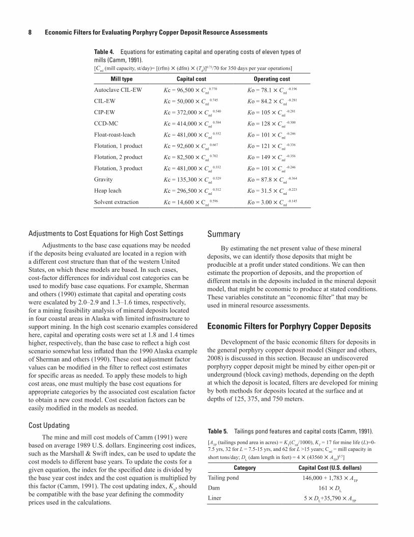
Table 4. Equations for estimating capital and operating costs of eleven types of mills (Camm, 1991).[Cml (mill capacity, st/day)= [(rfm) × (dfm) × (Td)]
0.75/70 for 350 days per year operations]
Mill type Capital cost Operating cost
Autoclave CIL-EW Kc = 96,500 × Cml0.770 Ko = 78.1 × Cml
-0.196
CIL-EW Kc = 50,000 × Cml 0.745 Ko = 84.2 × Cml
-0.281
CIP-EW Kc = 372,000 × Cml 0.540 Ko = 105 × Cml
-0.281
CCD-MC Kc = 414,000 × Cml 0.584 Ko = 128 × Cml
-0.300
Float-roast-leach Kc = 481,000 × Cml 0.552 Ko = 101 × Cml
-0.246
Flotation, 1 product Kc = 92,600 × Cml 0.667 Ko = 121 × Cml
-0.336
Flotation, 2 product Kc = 82,500 × Cml 0.702 Ko = 149 × Cml
-0.356
Flotation, 3 product Kc = 481,000 × Cml 0.552 Ko = 101 × Cml
-0.246
Gravity Kc = 135,300 × Cml 0.529 Ko = 87.8 × Cml
-0.364
Heap leach Kc = 296,500 × Cml 0.512 Ko = 31.5 × Cml
-0.223
Solvent extraction Kc = 14,600 × Cml 0.596 Ko = 3.00 × Cml
-0.145
Table 5. Tailings pond features and capital costs (Camm, 1991).
[ATP (tailings pond area in acres) = KT(Cml/1000), KT = 17 for mine life (L)=0-7.5 yrs, 32 for L = 7.5-15 yrs, and 62 for L >15 years; Cml = mill capacity in short tons/day; DL (dam length in feet) = 4 × (43560 × ATP)
0.5]
Category Capital Cost (U.S. dollars)
Tailing pond 146,000 + 1,783 × ATP
Dam 161 × DL
Liner 5 × DL+35,790 × ATP

Overview of Grade and Tonnage Models and Simplified Economic Filters 9
To develop the filters, two issues must be addressed: (1) selecting commodity prices for the analysis and (2) updating the original Camm equations to account for the change in prices since 1989 when the models were developed. After these issues are addressed, examples of the economic filter scenarios will be presented and discussed. Finally, we compare the results of our base porphyry copper deposit filters with the results of an economic analysis of copper mines developed between 1989 and 2008 (Doggett and Leville, 2010).
Commodity Prices and Calculation of Copper Equivalent Grades
Many porphyry copper deposits contain potentially recoverable byproduct metals; these byproduct metals include molybdenum, gold, and silver. The economic influence of byproduct metals is included in the economic filter by summing the recoverable value of the production of copper and the byproduct metals into the estimate of the value of ore per ton. This ore value can also be expressed as a copper equivalent grade. Copper equivalence is used by the mining industry to compare economic ore grades incorporating a variety of byproduct metals. Copper equivalence (CuEq) is calculated as:
CuEq (percent) = Gcu × [∑iRiViGi]/(RCuVCuGCu ), (10)
whereR is the respective metallurgical metal recovery
rate,V is time-averaged metal price/ton, andGi is metal commodity grade in percent of ore for
the suite of potentially recoverable com-modities, i, relative to copper (Cu).
The 1989–2008 average prices in 2008 U.S. dollars reported by Doggett and Leveille (2010) are used in the worked examples to calculate the value of ore per short ton and equivalent copper grade (table 6).
Updating the Engineering Cost ModelsLong and Singer (2001) and Long (2009) recognized
that, although Camm’s engineering cost equations provided a
robust basis for estimation of the costs of mining and milling deposits at an early stage of exploration, the original models, which were calibrated using 1989 data, needed to be updated to reflect the general change in price level. The cost updating methodology of Camm (1991, p. 4) was used to develop the economic filters described below. The Camm equations for cost parameters were updated from the 1989 calibration year using engineering cost index ratios, including the Marshall & Swift Index for mining and milling (Chemical Engineering, 1989–2008) and engineering cost index ratios derived from the “World Mine Cost Data Exchange” database (Mine Cost, 2009). Shafiee and others (2009) provided a 1980–2009 time-series analysis of average total costs of existing mining projects and operations, defined relative to Mine Cost cost indices for mining projects, including: (1) mill construction and labor costs; (2) machinery, heavy equipment, and line haul railroads (all services); (3) explosives, accessories, and miscellaneous materials and supplies; (4) capital costs (Canada trend); and (5) Marshall & Swift Index (mining, milling). The Shafiee and others (2009) study was developed to forecast trends in mining development and operating costs into the future. The variable used to update the cost parameters in the Camm equations was calculated as (average index 1989–2008)/(1989 index), similar to the method used to calculate the 1989–2008 average metal commodity prices that Doggett and Leveille (2010) used in their analysis. The time-averaged mining cost category indices derived from the Mine Cost database and Marshall & Swift Index had average values ranging from 1.25 to 1.27 for all of the cost group categories. An overall cost index (Ku) value of 1.26 was used to update the total operating and capital costs in the Camm equations, in conjunction with the 1989–2008 time averaged metal prices in table 6.
Porphyry Copper Deposit Economic Filter Example
Economic filters for porphyry copper deposits that are mined either by open-pit or block caving methods are presented in table 7. The following mine development conditions were assumed to apply: (1) the mine has 350 working days per year; (2) the depth to the top of the deposit, as specified in column D, is treated as an increase to the
Table 6. Metal prices and metallurgical recovery rates used in equivalent copper grade calculation and economic resource estimates.
[Source for average metal prices is Doggett and Leveille (2010), adjusted to 2008 U.S. dollars using U.S. Consumer Price Index Series U. Metallurgical recovery rates from Smith (1992, Table A-1, column 8)]
Value1989-2008
Copper Molybdenum Silver Gold
20-Year average price (2008 U.S. dollars)
Average price per short ton $3,460 $21,380 $233,921 $15,021,087 Metallurgical recovery 0.91 0.63 0.8 0.76

10 Economic Filters for Evaluating Porphyry Copper Deposit Resource Assessments
bottom depth of the open pit or shaft to the block caving mine; (3) the ore is beneficiated in a two-product flotation mill; (4) infrastructure in the cost model consists of a tailings pond and dam (the tailings pond is not lined); (5) the prices of metals and their metallurgical recovery rates are as given in table 6; (6) the cost models use a cost updating index (Ku) of 1.26, consistent with the base year criteria of the metal prices in table 6; (7) an increase in operating costs of 40 percent and capital costs of 80 percent is assumed for high cost mining settings; and (8) a 15-percent return on investment is assumed to attract capital. Table 7 is a worksheet that uses the updated cost models to estimate the net present values of 10 porphyry copper deposits (Singer and others, 2008) under four cover depth scenarios. Table 8 lists and briefly describes each column in the worksheet in table 7.
[Tables 7 and 8 are provided as an online electronic supplement.]
Table 7 presents the deposit characteristics, the assumed mining parameters, the estimated costs of mining, milling, and smelting the ore, and the net present values at a 15-percent rate of return for 10 porphyry copper deposits at four depth scenarios mined by either open pit (column AW) or block caving (column AX) methods. If either or both of the net present values is positive, the mining method with the larger present value is assumed to be used to mine the deposit, and the resources in the deposit can be considered to be economic. The final four columns of table 7 (columns BE through BH) contain the estimated recoverable resources of copper, molybdenum, gold, and silver in the deposit. A similar analysis can be performed for all deposits in a grade-tonnage model. The sum of resources that are in deposits evaluated as economic under each set of conditions divided by the total resources of the commodity in the grade-tonnage model defines the proportion of the undiscovered resources that are estimated to be economic to recover under the stated conditions.
Further, one may select some tonnages so as to cover a tonnage range of the deposits in the model and then vary their copper equivalent grade such that they have a net present value of zero, which is at the break-even cutoff grade of equivalent copper. These points can then be used to define a boundary between economic and uneconomic deposits. This limiting grade-tonnage boundary portrays the economic filter results for the stated depth and cost setting conditions.
Comparison of the Economic Filters with a Recent Analysis of the Economic Status of Copper Deposits
Doggett and Leveille (2010) report deposit-specific analysis of economic returns for 100 new copper mines brought into production from 1989 to 2008. Their analysis provides recent data on the economic characteristics of copper deposits that can be used for comparison with the results of the economic filters developed here with updated
Camm equations. The Doggett and Leveille (2010) analysis is based on reported tonnages, grades, and reported costs for individual copper deposits, assuming a minimum return of 8 percent to be considered economic. Although their analysis considered many types of copper deposits, many of the deposits are porphyry copper types, and most of the large tonnage-low grade deposits in their database that define the lower boundary of economic grades are porphyry copper deposits. Their economic analysis was in 2008 U.S. dollars using average commodity prices (1989–2008) for copper, gold, silver, zinc, molybdenum, and cobalt to calculate equivalent copper grade values (table 6). For porphyry copper deposits, gold, silver, and molybdenum are the relevant byproduct commodities. The break-even copper equivalent grade results from the simplified engineering cost economic filters calculated using the updated Camm cost equations under four depth-of-cover scenarios for porphyry copper deposits in the Singer and others (2008) database. The results are shown overlain on the grade-tonnage graph of Doggett and Leveille (2010) in figure 4.
Figure 4 demonstrates that the break-even grade-tonnage characteristics resulting from the updated simplified engineering cost filters, assuming current economic conditions and minimal cover, are consistent with the break-even grade-tonnage characteristics defining positive economic returns to development defined by Doggett and Leveille (2010). The updated economic filters show deposit depth/cost relations under current (2012) economic conditions consistent with recent industry experience and are considered appropriate to evaluate the economic status of porphyry copper mines under current economic conditions. Because metal prices and mining costs are similarly influenced by inflation and currency value trends, conclusions about relative costs and values of deposits of a particular type at varying depth are likely to be more stable over time than cost equation parameters estimated on any particular dataset of tonnage, grade, and prices (see Singer and others, 1998).
An interesting feature of the economic filters calculated by combining the open-pit and block caving models can be seen in the economic filter cutoff grades calculated for depths of 375 and 750 meters in the large tonnage part of the filter (fig. 4). The change in slope of these cutoff grades reflects a transition from open-pit to block caving mining in the model results.
Application of Economic Filters on Six Assessment Tract Results
In this section, the economic filters are applied to the resource assessment results of six porphyry copper deposit resource assessment tracts in North America. Table 9 lists the tract identifier codes, tract names, tract area, porphyry copper deposit model applied in the resource assessment, and a brief description of the geologic setting of porphyry copper deposits of each tract.

Application of Economic Filters on Six Assessment Tract Results 11
The selected tracts are shown in figure 5 by tract ID and name as given in table 9 and identified in text using tract ID. Two of the tracts are from an assessment of porphyry copper deposits in western Canada (CA–02, CA–04; Frost and others, 2011), three of the tracts are from an assessment of porphyry copper deposits in Mexico (MX–L1, MX–L2, MX–L3; Hammarstrom and others, 2010), and one tract is from an assessment of porphyry copper deposits in the Caribbean and Central America (CACB–T2; Gray and others, in press).
Several of the applications required the basic economic filters to be modified to be appropriate for porphyry copper deposit subtype models and for regions where existing infrastructure is markedly less available than that required for the basic economic filters based on costs in the western United States.
Economic Filters Applied to the Six Tract Areas
Undiscovered resources are estimated as:
(number of deposits) × (tonnage) × (ore grade) = (resource), (11)
where the number of deposits, tonnage, and ore grade features are described by probabilistic distributions (Singer and Menzie, 2010).
Monte Carlo simulation is used in the USGS three-part assessment method to estimate the mean undiscovered resource, based on the average of all simulation results. The economic resource is estimated as:
(resource) × (economic filter) = (economic resource), (12)
where resource is the mean undiscovered resource estimated by simulation; and the economic filter is the fraction of resources estimated to be economically recoverable based on the features of the grade-tonnage model used in the simulation, the depth distribution estimate for the undiscovered deposits, and adjustments for high cost settings if any are assumed for the assessment tract area.
The updated engineering cost equations were applied to the general porphyry copper deposit model and to two subtype models under both typical and high cost settings to define the economic filters that were used to calculate the fraction of deposits and the proportion of the resources within the deposit model that might be economic to recover at four cover depth intervals (0, 125, 375, and 750 m). The mine cost settings are: (1) typical cost setting with existing regional infrastructure to support mining and (2) a high cost setting typified by remote settings with a lack of infrastructure to support mining. For the high cost setting scenario used in
100.0
10.0
1.0
0.1
% C
uEq
Positive returns to developmentPositive returns to exploration
0.01 0.1 1 10 100 1,000 10,000Million metric tons (Mt) ore
EXPLANATION
0.01 Mt Copper
0.1 Mt Copper
1 Mt Copper
10 Mt Copper
0.01 Mt Copper
0.1 Mt Copper
1 Mt Copper
10 Mt Copper Economic status of copper
deposits 1989-2008Positive returns to explorationPositive returnsto development
Developed deposits
All others
DepositsPorphyry copper
Updated Camm (1991)cost model
Depth0 meters125 meters375 meters750 meters
Figure 4. Comparison of the cutoff grade calculated for porphyry copper deposits using updated simplified engineering cost models for open-pit and block caving mines as a function of deposit depth and ore tonnage. Also shown are the grade-tonnage features defining the case-study economics status of recently developed copper deposits (shown as large diamond symbols) from Doggett and Leveille (2010). % CuEq, percent copper equivalence, as defined in equation 10.

12 Economic Filters for Evaluating Porphyry Copper Deposit Resource Assessments
the examples, operating costs are assumed to be 40 percent higher than the typical case and capital costs are assumed to be 80 percent higher than the typical case; these factors can be modified to reflect estimates for specific areas. Table 10 shows the economic filter classification results for the general porphyry copper deposit model of Singer and others (2008), indicating both the fraction of undiscovered deposits and the fraction of ore metals in these deposits in the grade-tonnage model that are classified as economic under the different deposit depth and cost settings.
Uncertainty in estimated capital and operating costs influences the fraction of deposits and their contained resources classified as economic by the filter. The sensitivity of the expected number of economic deposits and amount of metal has been explored by applying cost escalation factors to the economic filter cost equations. An example using porphyry copper deposits under the assumption of typical mining conditions and a uniform depth distribution of undiscovered deposits from the surface to 1 km depth is shown in figure 6.
A 20 percent decrease in costs (base change, both capital and operating costs, equal to 0.8) results in a 41-percent increase in the number of deposits that are economic and a 10-percent increase in copper resources that are economic; a 20-percent increase in costs (base change equal to 1.2) results in a 29-percent decrease in the number of deposits that are economic and an 11-percent decrease in copper resources that are economic. The base rate change of number of economic deposits exceeds or is similar to the base rate change in costs, whereas the base rate change in amount of metal that is economic is about one-half that of the base rate change in costs. These smaller differences likely reflect the importance of the resource contribution from the giant deposits that are economic in nearly all settings.
Due to the influence of large tonnage deposits on mean deposit resources, the economic metal fractions exceed the percent of deposits classified as economic. The sensitivity analysis (fig. 6) indicates that the economic filter results for economic resources are not highly sensitive to modest uncertainty in the estimated capital and operating costs.
Table 9. Selected permissive tracts, porphyry copper deposit assessment, North America.
[Tract ID is used to identify specific tracts in figures and text; km2, square kilometers. General model is that of Singer and others (2008); Cu-Au subtype, copper-gold porphyry copper subtype (Singer and others, 2008); BCYK subtype, Canadian calc-alkaline porphyry copper ± gold ± molybdenite model (Frost and others, 2011)]
Tract ID Tract name/ location Coded ID Tract area (km2)
Porphyry copper deposit model Geologic setting for the tract
CA-02 Intermontane Island Arc (Canada)
003pCu2002 109,350 Cu-Au subtype Triassic to Jurassic alkaline igneous rocks of the Quesnel and Stikine accreted island-arc terranes.
CA-04 Cordilleran Continental Arc (Canada)
003pCu2004 684,140 BCYK subtype Jurassic to Eocene predominantly calc-alkaline igneous rocks of post-accretionary continental magmatic arcs.
MX-L1 Western Mexican Basin and Range (Mexico)
003pCu3006 74,140 General model Late Cretaceous to middle Eocene (Laramide) calc-alkaline magmatic arc rocks along the western margin of Mexico.
MX-L2 Sierra Madre Occidental (W) (Mexico)
003pCu3007 115,110 General model Late Cretaceous to middle Eocene (Laramide) calc-alkaline magmatic arc rocks in the Sierra Madre Occidental of northern Mexico.
MX-L3 Laramide Central Plateau (Mexico)
003pCu3008 58,720 General model Belt of Late Cretaceous to middle Eocene (Laramide) magmatic arc rocks in the eastern part of the Sierra Madre Occidental, eastern Mexican Basin and Range, and the Mesa Central of northern Mexico.
CACB-T2 Cocos (Central America) 003pCu4004 203,630 General model Miocene and younger volcanic arc rocks in southwest Mexico and Central America, including the modern Chiapanecan volcanic arc and Central American volcanic arc.

Application of Economic Filters on Six Assessment Tract Results 13
100°120°140°
50°
30°
10°
Laramide Central Plateau(MX–L3)
Western Mexican Basin and Range(MX–L1)
Intermontane Island-Arc Porphyry Cu-Au(CA–02)Cordilleran Continental Arc(CA–04)
Cocos(CACB–T2)
Sierra Madre Occidental(MX–L2)
EXPLANATION
PACIFIC OCEAN
Gulf of Mexico
Caribbean Sea
CANADA
UNITED STATES
MEXICO
GT
NI
CR
CO
HN
CU
SV
PA
0 500 1,000 KILOMETERS
0 250 500 MILES
Political boundary source: U.S. Department of State (2009)Projection: North American Lambert Conformal Conic;Central meridian 65° W; Latitude of Origin 35° N
BZ
Figure 5. Selected permissive tracts for porphyry copper deposits in North America. Tract identifiers, names, and descriptions are given in table 9. GT, Guatemala; BZ, Belize; SV, El Salvador; HN, Honduras; NI, Nicaragua; CR, Costa Rica; PA, Panama; CO, Columbia; CU, Cuba.

14 Economic Filters for Evaluating Porphyry Copper Deposit Resource Assessments
Application of the Economic Filter to Estimates of Undiscovered Resources in the Six Tracts
Quantitative resource assessments are model-based estimates using information available at the time the assessment is conducted and the assumptions adopted by the assessment team. An economic filter applied to quantitative assessment results creates a scenario based on assumed costs, prices, and geologic conditions, such as depth and setting of the undiscovered deposits.
USGS three-part quantitative assessments provide estimates of in-ground undiscovered resources on a tract basis. In the USGS global assessment of undiscovered porphyry
Tables 11 and 12 present results from applying economic filters to the porphyry copper-gold deposit subtype model (model 20c, Cox, 1986; using grade-tonnage data from Singer and others, 2008) and the calc-alkaline porphyry Cu-Mo-Au deposits of the Canadian Cordillera subtype model (Frost and others, 2011), abbreviated as the BCYK model in the following examples. Owing to the presence of giant deposits, the copper-gold subtype model (table 11) has similar economic filter characteristics to the general porphyry copper deposit model (table 10). Owing to the lower tonnages and grades of the BCYK subtype model, the economic filter results are lower (table 12). For both models, individual economic metal recovery rates are given for contained copper, molybdenum, gold, and silver resources.
Table 10. Economic filter results for the general porphyry copper deposit model (Singer and others, 2008) assuming the specified metal recovery rates for each commodity.[Cu, copper; Mo, molybdenum; Au, gold; and Ag, silver. The fraction of undiscovered deposits and their contained metal resources classified as economic according to filter criteria are shown. Metal recovery rate is the product of the ore recovery rate times the metallurgical recovery rate for each commodity; the high cost setting assumes that operating costs and capital costs are 40 and 80 percent higher, respectively, than typical costs. Deposit depth is the depth to the top of ore]
Depth (meters) Cost settingEconomic fraction of resource simulation
Deposits Cu Mo Au Ag
0 Typical 0.780 0.808 0.560 0.676 0.718
125 Typical 0.633 0.791 0.552 0.657 0.707
375 Typical 0.367 0.729 0.511 0.570 0.655
750 Typical 0.192 0.581 0.438 0.439 0.546
0 High cost 0.436 0.734 0.517 0.590 0.648
125 High cost 0.318 0.688 0.497 0.557 0.625375 High cost 0.142 0.554 0.424 0.411 0.539
750 High cost 0.038 0.358 0.310 0.196 0.361
Metal recovery rate 0.82 0.57 0.68 0.72
Figure 6. Sensitivity of expected number of economic deposits and amount of copper resources in porphyry copper deposits composing the general porphyry copper model of Singer and others (2008) with respect to possible changes in expected base operating and capital costs, assuming a uniform depth distribution of undiscovered deposits.
0.4
0.6
0.8
1.2
1.4
1.6
1.8
1
0.6 0.8 1 1.2 1.4
Chan
ge in
exp
ecte
d am
ount
Change to base expected costs
CopperDeposits
EXPLANATION

Application of Economic Filters on Six Assessment Tract Results 15
copper deposits, an expert panel estimated the number of undiscovered deposits likely to occur in tracts at three or more different confidence levels. A probability distribution of deposits was calculated that is consistent with the estimates of the panel (Root and others, 1992). A Monte Carlo simulation combines the distribution of number of undiscovered deposits with the grade-tonnage model or submodel appropriate for each tract, to generate resource estimates at different confidence levels (Singer, 1993a). An economic filter for both open-pit and block caving mining methods was then applied to the simulated undiscovered resources estimated for each
tract. For each tract, the assessment process provides estimates of undiscovered deposits at different confidence levels and their relative distribution by depth, a grade-tonnage model that is used to simulate the undiscovered resources contained in these deposits, and a cost setting parameter based on tract geology and infrastructure features, all combined to estimate undiscovered economic resources.
The simple tract-based economic filter scenario described below is based on information in the grade-tonnage model applied to the tract and some additional general tract setting information that can be estimated by the assessment panel. In
Table 11. Economic filter results for the Cu-Au porphyry copper deposit subtype (Singer and others, 2008) assuming the specified metal recovery rates for each commodity.[Cu, copper; Mo, molybdenum; Au, gold; and Ag, silver. The fraction of undiscovered deposits and their contained metal resources classified as economic accord-ing to filter criteria are shown. Metal recovery rate is the product of the ore recovery rate times the metallurgical recovery rate for each commodity; the high cost setting assumes that operating costs and capital costs are 40 and 80 percent higher, respectively, than typical costs. Deposit depth is the depth to the top of ore]
Depth (meters) Cost settingEconomic fraction of resource simulation
Deposits Cu Mo Au Ag
0 Typical 0.852 0.813 0.566 0.674 0.714
125 Typical 0.670 0.793 0.556 0.649 0.692
375 Typical 0.374 0.716 0.506 0.577 0.616
750 Typical 0.235 0.611 0.494 0.432 0.538
0 High cost 0.487 0.747 0.517 0.586 0.645
125 High cost 0.348 0.709 0.502 0.548 0.615
375 High cost 0.157 0.577 0.472 0.405 0.525
750 High cost 0.043 0.318 0.219 0.178 0.384
Metal recovery rate 0.82 0.57 0.68 0.72
Table 12. Economic filter results for the BCYK porphyry copper deposit subtype assuming the specified metal recovery rates for each commodity.[BCYK subtype, Canadian calc-alkaline porphyry copper±gold±molybdenite model (Frost and others, 2011). Cu, copper; Mo, molybdenum; Au, gold; and Ag, silver. The fraction of undiscovered deposits and their contained metal resources classified as economic according to filter criteria are shown. Metal recovery rate is the product of the ore recovery rate times the metallurgical recovery rate for each commodity; the high cost setting assumes that operating costs and capital costs are 40 and 80 percent higher, respectively, than typical costs. Deposit depth is the depth to the top of ore]
Depth (meters) Cost settingEconomic fraction of resource simulation
Deposits Cu Mo Au Ag
0 Typical 0.647 0.739 0.513 0.556 0.689
125 Typical 0.382 0.662 0.486 0.506 0.673
375 Typical 0.059 0.295 0.228 0.088 0.127
750 Typical 0.029 0.226 0.130 0.005 0.127
0 High cost 0.088 0.323 0.249 0.111 0.154
125 High cost 0.029 0.226 0.130 0.005 0.127
375 High cost 0.000 0.000 0.000 0.000 0.000750 High cost 0.000 0.000 0.000 0.000 0.000Metal recovery rate 0.82 0.57 0.68 0.72

16 Economic Filters for Evaluating Porphyry Copper Deposit Resource Assessments
the examples presented here, the simple economic filter analysis is applied to the mean amount of undiscovered resources esti-mated by the Monte Carlo simulation. This approach allows the economic filter criteria to be defined based on the actual deposits in the grade-tonnage model and not on the characteristics of each simulated deposit resulting from the Monte Carlo simulation (that is, the economic filter only has to determine the potentially economic resource fraction once for each unique grade-tonnage model using the depth and cost-setting scenario criteria). However, it is possible to implement the economic filter analysis as part of the Monte Carlo simulation process to estimate the full distribution of estimated economic resources.
The depth distribution criteria of undiscovered deposits was implemented by each assessment team estimating the proportion of the undiscovered porphyry copper deposits in the tract likely to occur in three depth intervals, for example 0–250 m, 250–500 m, and 500–1,000 m. For porphyry copper deposits, and prob-ably many other deposit types, the likely undiscovered deposit distribution will be a function of recognizable tract features. Porphyry copper deposits are commonly associated with shal-lowly emplaced (1–5 km) igneous bodies of intermediate to felsic composition. Porphyry copper deposits have been interpreted to form slightly above the depth (pressure) of the critical point of their associated source fluids (Burnham, 1981, 1985). Under these depth-pressure conditions, fluid exsolving from the magma provides the mechanical energy to produce the extensive hydro-fractured vein-breccia network that is an ore-host characteristic of porphyry deposits. The assignment of proportions of deposits to depth classes for individual tracts depends on an analysis of the characteristics of the existing igneous bodies as well as the uplift, erosion, and younger cover depositional history of the tract. Many deposit types may have depth distributions that could be estimated by assessors using mineralizing system concepts appropriate for the deposit type of interest, or a default assumption of uniform depth distribution could be assumed.
The cost settings of each tract were defined by the assessment team as the estimated fraction of the tract that was likely to have “typical” mining costs and the fraction of the tract that was likely to have “high” mining costs. The economic filter then consists of the percentages of deposits and undiscovered resources (Ru) estimated to be economic for the grade-tonnage model and cost settings of each tract. The tract-scale economic filter is calculated as follows, for economic recovered copper:
Potential economic recovered Cu = Ru,cu[∑i∑j(DDFi)(SFj)(MCuFij)], (13)
where Ru,cu is mean amount undiscovered Cu
resource from the Monte Carlo simulation, DDFi is deposit depth distribution fraction in
depth interval i (defined by assessors), SFj is cost setting fraction estimate for setting
j (defined by assessors), and MCuFij is fraction of economic Cu resource in
deposit model, as a function of depth and cost settings.
The fractions of the number of undiscovered deposits that are potentially economic in the tract is calculated as follows:
Economic deposit fraction (EDF) = [∑i∑j(DDFi)(SFj)(MDFij)], (14)
where DDFi is deposit depth distribution fraction in
depth interval i (defined by assessors), SFj is cost setting fraction estimate for setting
j (defined by assessors), and MDFij is fraction of the number of deposits
classed economic in the grade-tonnage model by the economic filter, as a function of depth and cost setting parameters.
The fraction of undiscovered resources classed as economic for each depth and tract setting criteria are tabulated in table 10 for the general porphyry copper grade-tonnage model. Tables 11 and 12 present the same information for the copper-gold porphyry copper subtype model and for the BCYK porphyry copper subtype model, respectively.
These economic resource fractions are used in conjunction with assessment team estimates of undiscovered deposit fractions in the depth groups and tract settings to estimate the economic fraction of the mean undiscovered resource estimates by tract. In addition to an estimate of mean economic resources, the probability of no economic resources in a tract can be estimated. The probability of no economic resource occurring in the tract is a binomial probability function involving: (1) the probability of no deposits occurring in the tract estimated by the assessment panel and as a result of Monte Carlo simulation, (2) the fraction of deposits in the grade-tonnage model that is classified by the economic filter as economic under tract conditions (EDF), and (3) the mean number of undiscovered deposits in the tract. The Monte Carlo simulation probability of no deposits occurring in the tract (MC0) is based on the assessment panel estimates of undiscovered deposit numbers at different confidence levels, expressed as the probability of zero deposits in the Monte Carlo simulation output.
Pf = MC0 + (1–MC0) (1–EDF)n, (15)
where Pf is the probability of no economic resource
in the tract (probability of failure), (MC0) is the Monte Carlo probability of no
resources occurring in the tract, (1–EDF) is the probability that a simulated
deposit will be subeconomic under tract conditions, and
n is the estimate of mean undiscovered deposits for the tract (which is an estimate of the number of sample trials for the tract).

Conclusions 17
Examples of Tract-Based Economic Filter Results
A simple economic filter scenario has been developed for six porphyry copper deposit tracts in North America included as part of the USGS Global Mineral Resource Assessment (Schulz and Briskey, 2003). The selected tract locations are shown in figure 5 and tract characteristics are summarized in table 9. The tract ID code in table 9 is used to identify the tracts discussed below. Four tracts in Mexico and Central America (MX–L1, MX–L2, and MX–L3, and CACB–T2) used the general porphyry copper deposit model for assessment. Tract CA–02 in Canada used the Cu-Au subtype model (Cox, 1986; Singer and others, 2008) and tract CA–04 in Canada used the BCYK subtype model (Frost and others, 2011).
Examples of depth distribution estimates and mining cost settings for each tract are given below and summarized in table 13. Active mining operations of a variety of types and scales are common in the northern Mexico region containing tracts MX–L1, MX–L2, and MX–L3 (Hammarstrom and others, 2010), and the climate and infrastructure base is conducive for mine development. These tracts are classed as “typical” setting status. Tract MX–L2 is the most productive porphyry tract in Mexico and is at an optimal exhumation level for discovery of porphyry deposits based on known deposits and the distribution of permissive intrusive and volcanic rocks (Hammarstrom and others, 2010). The undiscovered deposit distribution in MX–L2 is likely to be skewed toward shallow depths compared with that expected by a uniform depth distribution (40 percent <250 m, 30 percent 250–500 m, and 30 percent >500 m; table 13). Tract MX–L1 has similar characteristics to MX–L2, but is dominated by exposed permissive volcanic rocks and has more extensive younger cover. For the MX–L1 tract, the undiscovered deposit distribution is likely to be skewed slightly toward mid-level depths (20 percent <250 m, 40 percent 250–500 m, and 40 percent >500 m; table 13). Tract MX–L3 has very few known porphyry copper deposits, but has a number of polymetallic and epithermal deposits that might be associated with porphyry systems at depth. Exposed Laramide-age intrusions are scarce, but are inferred at depth based on epithermal systems and aeromagnetic anomalies. Younger Tertiary and Quaternary volcanic rocks and sediments cover parts of the tract. For tract MX–L3, the depth distribution of undiscovered porphyry deposits is likely to be skewed toward greater depths and with few deposits in the shallow depth interval (5 percent <250 m, 25 percent 250–500 m, and 70 percent >500 m; table 13).
Tract CACB–T2 covers part of southernmost Mexico and extends through Central America. This tract contains a few large active mines. However, most of the tract is covered by rain forest, and large remote areas in the tract have little infrastructure development (Gray and others, in press). Tract CACB–T2 was classified as “high cost”
setting. The tract covers a large area, and because the undiscovered deposit depth distribution is uncertain, has a uniform deposit distribution with depth (25 percent <250 m, 25 percent 250–500 m, and 50 percent >500 m; table 13) was assumed.
The BCYK subtype grade-tonnage model (Frost and others, 2011) is applied to the CA–04 tract in Canada (Mihalasky and others, 2011). The CA–04 tract is dominated by volcanic rocks, and the depth distribution of undiscovered deposits is likely to be skewed slightly toward greater depths than expected by a uniform depth distribution. Two cost filters were applied to this tract: (1) typical mining cost setting and (2) a 50:50 percent typical and high cost setting allocation to illustrate the influence of the cost variable for this deposit subtype.
The Cu-Au subtype model is applied to tract CA–02 in Canada (Mihalasky and others, 2011). Tract CA–02 has a mix of exposed permissive volcanic and plutonic rocks; the depth distribution of undiscovered deposits is likely to be skewed slightly toward shallower depths than a uniform depth distribution. Much of this tract is in remote areas with high relief. The assessment team classified 40 percent of the tract as having typical mining cost and 60 percent as high cost mining for this example.
The results are tabulated in table 13. The individual commodity metal recovery rates listed in table 6 were used in the calculations.
ConclusionsMineral resource estimates are dominated by the larger
tonnage deposits in the grade-tonnage model applied in the assessment process. The largest tonnage deposits that make up 1 percent of all porphyry copper deposits (Singer and others, 2008) account for 30 percent of the copper resource, those that make up 20 percent of the deposits account for 80 percent of the copper resource, and the smallest 50 percent of the deposits account for less than 5 percent of the copper resource. As a result, the economic filter results are not sensitive to economic-subeconomic discrimination criteria for low tonnage deposits.
The grade-tonnage break-even curve predicted using cost updated Camm equations for open-pit porphyry copper deposits is consistent with the grade-tonnage break-even economic curve defined by a study of copper mines of all types developed from 1989 to 2008 (Doggett and Leveille, 2010). The agreements between these two different datasets provide evidence that the price-adjusted Camm equations provide a useful rudimentary economic filter to evaluate the economic status of porphyry copper and other mineral deposits under current, and potentially future, economic conditions.
The economic filter can be easily applied to mean undiscovered resource results outside of the Monte Carlo simulation process. In addition, it provides an estimate of
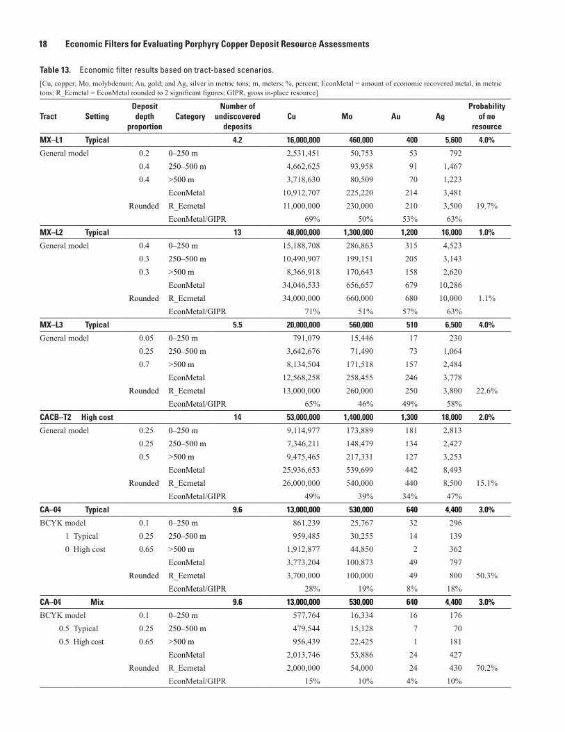
18 Economic Filters for Evaluating Porphyry Copper Deposit Resource Assessments
Table 13. Economic filter results based on tract-based scenarios.[Cu, copper; Mo, molybdenum; Au, gold; and Ag, silver in metric tons; m, meters; %, percent; EconMetal = amount of economic recovered metal, in metric tons; R_Ecmetal = EconMetal rounded to 2 significant figures; GIPR, gross in-place resource]
Tract SettingDeposit depth
proportionCategory
Number of undiscovered
depositsCu Mo Au Ag
Probability of no
resource
MX–L1 Typical 4.2 16,000,000 460,000 400 5,600 4.0%
General model 0.2 0–250 m 2,531,451 50,753 53 7920.4 250–500 m 4,662,625 93,958 91 1,4670.4 >500 m 3,718,630 80,509 70 1,223
EconMetal 10,912,707 225,220 214 3,481Rounded R_Ecmetal 11,000,000 230,000 210 3,500 19.7%
EconMetal/GIPR 69% 50% 53% 63%MX–L2 Typical 13 48,000,000 1,300,000 1,200 16,000 1.0%
General model 0.4 0–250 m 15,188,708 286,863 315 4,5230.3 250–500 m 10,490,907 199,151 205 3,1430.3 >500 m 8,366,918 170,643 158 2,620
EconMetal 34,046,533 656,657 679 10,286Rounded R_Ecmetal 34,000,000 660,000 680 10,000 1.1%
EconMetal/GIPR 71% 51% 57% 63%MX–L3 Typical 5.5 20,000,000 560,000 510 6,500 4.0%
General model 0.05 0–250 m 791,079 15,446 17 2300.25 250–500 m 3,642,676 71,490 73 1,0640.7 >500 m 8,134,504 171,518 157 2,484
EconMetal 12,568,258 258,455 246 3,778Rounded R_Ecmetal 13,000,000 260,000 250 3,800 22.6%
EconMetal/GIPR 65% 46% 49% 58%CACB–T2 High cost 14 53,000,000 1,400,000 1,300 18,000 2.0%
General model 0.25 0–250 m 9,114,977 173,889 181 2,8130.25 250–500 m 7,346,211 148,479 134 2,4270.5 >500 m 9,475,465 217,331 127 3,253
EconMetal 25,936,653 539,699 442 8,493Rounded R_Ecmetal 26,000,000 540,000 440 8,500 15.1%
EconMetal/GIPR 49% 39% 34% 47%CA–04 Typical 9.6 13,000,000 530,000 640 4,400 3.0%
BCYK model 0.1 0–250 m 861,239 25,767 32 2961 Typical 0.25 250–500 m 959,485 30,255 14 1390 High cost 0.65 >500 m 1,912,877 44,850 2 362
EconMetal 3,773,204 100,873 49 797Rounded R_Ecmetal 3,700,000 100,000 49 800 50.3%
EconMetal/GIPR 28% 19% 8% 18%CA–04 Mix 9.6 13,000,000 530,000 640 4,400 3.0%
BCYK model 0.1 0–250 m 577,764 16,334 16 1760.5 Typical 0.25 250–500 m 479,544 15,128 7 700.5 High cost 0.65 >500 m 956,439 22,425 1 181
EconMetal 2,013,746 53,886 24 427Rounded R_Ecmetal 2,000,000 54,000 24 430 70.2%
EconMetal/GIPR 15% 10% 4% 10%

References Cited 19
the probability of no economic resources occurring in a tract based on the fraction of deposits in the grade-tonnage model that are classified as subeconomic under tract scenario conditions and the probability of no deposits occurring in the tract. The economic filter could be applied during the Monte Carlo simulation to estimate the complete distribution of economic resources. However, the current simulation program would require substantial modification to implement this option.
The grade-tonnage distributions of porphyry copper deposits provide insights into the likely future patterns of resource supplies needed to satisfy increasing consumption of mineral commodities on a global scale. Deposit tonnage, through its influence on total contained metal (Singer and Menzie, 2010), mine capacity, mine life, and economic status, has a profound influence on the pattern of resource supply. Based on the frequency and range of the grade and tonnages of known porphyry copper deposits, global copper supply will continue to be dominated byproduction from a small number of giant deposits (Singer, 1995). Assessment results of undiscovered resources and continuing mineral deposit discoveries suggest that mineral resource supply will not limit growth in the near future (Menzie and others, 2005). However, the bulk of global resource supply will likely continue to come from a small number of giant tonnage deposits, and this limitation on resource supply may increase in the future, because an increasing proportion of new deposit discoveries are likely to occur in remote areas and concealed deep beneath covering rock and sediments. Extensive mineral exploration activity likely will be required to meet future resource demand, because those deposits will be hard to find and more costly to mine.
References Cited
Burnham, C.W., 1981, Physicochemical constraints on porphyry mineralization: Geological Society of Arizona Digest, v. 14, p. 71–77.
Burnham, C.W., 1985, Energy release in subvolcanic environments—Implications for breccias formation: Economic Geology, v. 80, p. 1515–1522.
Camm, T.W., 1991, Simplified cost models for prefeasibility mineral evaluations: U.S. Bureau of Mines Information Circular 9298, 35 p.
Camm, T.W., 1994, Simplified cost models for prefeasibility mineral evaluations: Mining Engineering, June 1994, p. 559–562.
Chemical Engineering, 1989–2009, Economic indicators [online]: Chemical Engineering, accessed October 10, 2011, at www.che.com.
Cox, D.P., 1986, Descriptive model of porphyry Cu-Au, in Cox, D.P., and Singer, D.A., eds., Mineral deposit models: U.S. Geological Survey Bulletin 1693, p. 110, available at http://pubs.usgs.gov/bul/b1693/.
Cox, D.P., Barton, P.R., and Singer, D.A., 1986, Introduction, in Cox, D.P., and Singer, D.A., eds., Mineral deposit models: U.S. Geological Survey Bulletin 1693, p. 1–10.
Doggett, M.D., and Leveille, R.A., 2010, Assessing the returns to copper exploration, 1989–2008: Exploration and Mining Geology, v. 19, no. 1–2, p. 23–33.
Table 13. Economic filter results based on tract based scenarios.—Continued[Cu, copper; Mo, molybdenum; Au, gold; and Ag, silver in metric tons; m, meters; %, percent; EconMetal = amount of economic recovered metal, in metric tons; R_Ecmetal = EconMetal rounded to 2 significant figures; GIPR, gross in-place resource]
Tract SettingDeposit depth
proportionCategory
Number of undiscovered
depositsCu Mo Au Ag
Probability of no
resource
CA-02 MIX 7 22,000,000 130,000 1,600 7,400 3.0%
Cu-Au model 0.3 0–250 m 4,901,539 20,422 283 1,4330.4 Typical 0.3 250–500 m 4,177,060 18,948 224 1,2460.6 High cost 0.4 >500 m 3,828,717 17,109 179 1,320
EconMetal 12,907,316 56,479 685 3,998
Rounded R_Ecmetal 13,000,000 56,000 690 4,000 12.0%
EconMetal/GIPR 59% 43% 43% 54%

20 Economic Filters for Evaluating Porphyry Copper Deposit Resource Assessments
Drew, L.J., Singer, D.A., Menzie, W.D., and Berger, B.R., 1999, Mineral-resource assessment—State of the art: Geologica Hungarica Series Geologica, v. 24, p. 31–40.
Frost, T.P., Bookstrom, A.A., and Mihalasky, M.J., 2011, Grade and tonnage model for calc-alkaline porphyry Cu+Mo+Au deposits of the Canadian Cordillera, in Mihalasky, M.J., Bookstrom, A.A., Frost, T.P., and Ludington, S.D., with contributions from Logan, J.M., Panteleyev, Andre, and Abbott, Grant, Porphyry copper assessment of British Columbia and Yukon Territory, Canada: U.S. Geological Survey Scientific Investigations Report 2010–5090–C, p. 118–125, available at http://pubs.usgs.gov/sir/2010/5090/c/.
Gray, Floyd, Hammarstrom, J.M., Ludington, S.D., Zürcher, Lukas, Nelson, C.E., Robinson, G.R., Jr., Miller, R.J., and Moring, B.C., in press, Porphyry copper assessment of the Caribbean and Central America: U.S. Geological Survey Scientific Investigations Report 2010–5090–I.
Hammarstrom, J.M., Robinson, G.R., Jr., Ludington, S.D., Gray, Floyd, Drenth, B.J., Cendejas-Cruz, Francisco, Espinosa, Enrique, Pérez-Segura, Efrén, Valencia-Moreno, Martín, Rodríguez-Castañeda, José Luis, Vásquez-Mendoza, Rigoberto, and Zürcher, Lukas, 2010, Porphyry copper assessment of Mexico: U. S. Geological Survey Scientific Investigations Report 2010–5090–A, 176 p., available at http://pubs.usgs.gov/sir/2010/5090/a/.
Harris, D.P., 1990, Mineral exploration decisions: New York, John Wiley and Sons, 436 p.
Harris, D.P., and Rieber, Michael, 1993, Evaluation of the United States Geological Survey’s three-step assessment methodology: U.S. Geological Survey Open File Report 93–258A, 675 p.
Long, K.R., 2009, A test and re-estimation of Taylor’s empirical capacity-reserve relationship: Natural Resources Research, v. 18, no. 1, p. 57–63.
Long, K.R., and Singer, D.A., 2001, A simplified economic filter for open-pit mining and heap-leach recovery of copper in the United States: U.S. Geological Survey Open-File Report 01–218, 21 p., available at http://geopubs.wr.usgs.gov/open-file/of01-218/.
Menzie, W.D., Singer, D.A., and DeYoung, J.H., Jr., 2005, Mineral resources and consumption in the twenty-first century, in Simpson, R.D., Torman, M.A., and Ayres, R.U., eds., Scarcity and growth revisited—Natural resources and the environment in the new millennium: Washington, D.C., Resources for the Future, p. 33–53.
Mihalasky, M.J., Bookstrom, A.A., Frost, T.P., and Ludington, S.D., with contributions from Logan, J.M., Panteleyev, Andre, and Abbott, Grant, 2011, Porphyry copper assessment of British Columbia and Yukon Territory, Canada: U.S. Geological Survey Scientific Investigations Report 2010–5090–C, 128 p., available at http://pubs.usgs.gov/sir/2010/5090/c/.
Mine Cost, 2009, World mine cost data exchange [online]: accessed October 10, 2011, at http://www.minecost.com.
Pannell, D.J., 1997, Sensitivity analysis of normative economic models—Theoretical framework and practical strategies: Agricultural Economics, v. 16, p. 139–152.
Root, D.H., Menzie, W.D., and Scott, W.A., 1992, Computer Monte Carlo simulation in quantitative resource estimation: Nonrenewable Resources, v. 1, no. 2, p. 125–138.
Schulz, K.J., and Briskey, J.A., 2003, The Global Mineral Resource Assessment Project: U.S. Geological Survey Fact Sheet 053–03, 4 p., available at http://pubs.usgs.gov/fs/fs053-03/.
Shafiee, S., Nehring, M., and Topal, E., 2009, Estimating average total cost of open pit coal mines in Australia: Australian Mining Technology Conference, October 27–28, 2009, p. 134–145, accessed November 3, 2011, at http://www.infomine.com/publications/docs/Shafiee2009a.pdf.
Sherman, G.E., Coldwell, J.R., Herzog, Denise, and Meyer, M.P., 1990, Analysis of Balboa Bay, Beluga, Point MacKenzie, and Lost River as port sites for use by the mineral industry: U.S. Bureau of Mines Open-File Report 36–90, 54 p.
Singer, D.A., 1993a, Basic concepts in three-part quantitative assessments of undiscovered mineral resources: Nonrenewable Resources, v. 2, no. 2, p. 69–81.
Singer, D.A., 1993b, Development of grade and tonnage models for different deposit types, in Kirkham, R.V., Sinclair, W.D., Thorpe, R.I., and Duke, J.M., eds., Mineral deposit modeling: Geological Association of Canada, Special Paper 40, p. 21–30.
Singer, D.A., 1995, World-class base and precious metal deposits—A quantitative analysis: Economic Geology, v. 90, no. 1, p. 88–104.
Singer, D.A., 2010, Progress in integrated quantitative mineral resource assessments: Ore Geology Reviews, v. 38, p. 242–250.
Singer, D.A., and Menzie, W.D., 2010, Quantitative mineral resource assessments—An integrated approach: New York, Oxford University Press, 219 p.

References Cited 21
Singer, D.A., Menzie, W.D., and Long, K.R., 1998, A simplified economic filter for open-pit gold-silver mining in the United States: U.S. Geological Survey Open-File Report 98–207, 10 p.
Singer, D.A., Menzie, W.D., and Long, K.R., 2000, A simplified economic filter for underground mining of massive sulfide deposits: U.S. Geological Survey Open-File Report 00–349, 20 p.
Singer, D.A., Berger, V.I., and Moring, B.C., 2008, Porphyry copper deposits of the world—Database, map, and grade and tonnage models, 2008: U.S. Geological Survey Open-file Report 2008–1155, 45 p., available at http://pubs.usgs.gov/of/2008/1155/.
Smith, R.C., 1992, PREVAL—Prefeasibility software program for evaluating mineral properties, version 1.01: U. S. Bureau of Mines Information Circular 9307, 35 p.
Taylor, H.K., 1978, Mine valuation and feasibility studies, in Hoskins, J.R., and Green, W.R., eds., Mineral industry costs (2nd ed.): Spokane, Washington, Northwest Mining Association, p. 1–17.
Taylor, H.K., 1986, Rates of working mines—A simple rule of thumb: Transactions of the Institution of Mining and Metallurgy, v. 95, p. A203–A204.
U.S. Department of State, 2009, Small-scale digital international land boundaries (SSIB)-Lines, edition 10, and polygons, beta edition 1, in Boundaries and sovereignty encyclopedia (B.A.S.E.): U.S. Department of State, Office of the Geographer and Global Issues.
U.S. Geological Survey National Mineral Resource Assessment Team, 2000, 1998 assessment of deposits of gold, silver, copper, lead, and zinc in the United States: U.S. Geological Survey Circular 1178, 21 p.
Produced in the Menlo Park Publishing Service Center, CaliforniaManuscript approved for publication, August 14, 2012Edited by Gail SladekLayout and design by Vivian Tuong and Jeanne S. DiLeo

Robinson and Menzie—
Economic Filters for Evaluating Porphyry Copper D
eposit Resource Assessm
ents—Scientific Investigations Report 2010–5090–H
, ver. 1.2