Embed Size (px)
Citation preview

ECONOMIC FACTORS AFFECTING THE INCREASE IN OBESITY
IN THE UNITED STATES: DIFFERENTIAL RESPONSE TO PRICE
A Paper Submitted to the Graduate Faculty
of the North Dakota State University
of Agriculture and Applied Science
By
Hélène de Chastenet
In Partial Fulfillment of the Requirements for the Degree of
MASTER OF SCIENCE
Major Department: Agribusiness and Applied Economics
June 2005
Fargo, North Dakota
iii
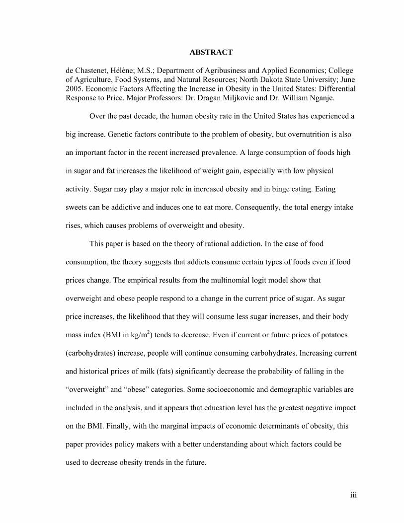
ABSTRACT
de Chastenet, Hélène; M.S.; Department of Agribusiness and Applied Economics; College of Agriculture, Food Systems, and Natural Resources; North Dakota State University; June 2005. Economic Factors Affecting the Increase in Obesity in the United States: Differential Response to Price. Major Professors: Dr. Dragan Miljkovic and Dr. William Nganje. Over the past decade, the human obesity rate in the United States has experienced a
big increase. Genetic factors contribute to the problem of obesity, but overnutrition is also
an important factor in the recent increased prevalence. A large consumption of foods high
in sugar and fat increases the likelihood of weight gain, especially with low physical
activity. Sugar may play a major role in increased obesity and in binge eating. Eating
sweets can be addictive and induces one to eat more. Consequently, the total energy intake
rises, which causes problems of overweight and obesity.
This paper is based on the theory of rational addiction. In the case of food
consumption, the theory suggests that addicts consume certain types of foods even if food
prices change. The empirical results from the multinomial logit model show that
overweight and obese people respond to a change in the current price of sugar. As sugar
price increases, the likelihood that they will consume less sugar increases, and their body
mass index (BMI in kg/m2) tends to decrease. Even if current or future prices of potatoes
(carbohydrates) increase, people will continue consuming carbohydrates. Increasing current
and historical prices of milk (fats) significantly decrease the probability of falling in the
“overweight” and “obese” categories. Some socioeconomic and demographic variables are
included in the analysis, and it appears that education level has the greatest negative impact
on the BMI. Finally, with the marginal impacts of economic determinants of obesity, this
paper provides policy makers with a better understanding about which factors could be
used to decrease obesity trends in the future.

iv
ACKNOWLEDGMENTS
I would like to thank my major advisors, Dr. Dragan Miljkovic and Dr. William
Nganje, for their support and guidance. I appreciate the help from my committee members,
Dr. Cheryl Devuyst and Dr. Jane Edwards, for their constructive comments throughout the
academic year.
I would like to thank my parents and my friends, especially Prashant Varma and Dr.
& Mrs. Croll, for their encouragement.

v
TABLE OF CONTENTS
ABSTRACT.......................................................................................................................... iii
ACKNOWLEDGMENTS .................................................................................................... iv
LIST OF TABLES............................................................................................................... vii
LIST OF FIGURES ............................................................................................................viii
CHAPTER 1. INTRODUCTION .......................................................................................... 1
Background/Problem Statement ........................................................................................ 1
Justification of the Study ................................................................................................... 4
Description of the Study .................................................................................................... 5
Study Objectives and Hypothesis ...................................................................................... 6
Outline ............................................................................................................................... 6
CHAPTER 2. LITERATURE REVIEW............................................................................... 7
Trends of BMI in the World and in the United States ....................................................... 7
Does Eating Sugar Make People Obese?......................................................................... 13
CHAPTER 3. A MODEL OF RATIONAL ADDICTION ................................................. 21
CHAPTER 4. EMPIRICAL METHODS AND PROCEDURES........................................ 26
CHAPTER 5. EMPIRICAL RESULTS AND DISCUSSIONS.......................................... 29
Data and Estimation Procedures...................................................................................... 29
Empirical Results............................................................................................................. 32
CHAPTER 6. CONCLUSIONS .......................................................................................... 41
Summary of Problem....................................................................................................... 41
Summary of Objectives ................................................................................................... 41
vi
Summary of Methodology............................................................................................... 42
Summary of Results......................................................................................................... 42
Study Limitations............................................................................................................. 43
Implication for Further Study .......................................................................................... 44
REFERENCES CITED........................................................................................................ 45
APPENDIX A. SUPPLEMENT RESULTS........................................................................ 52

vii
LIST OF TABLES
Table Page
1. Prevalence of overweight, obesity, and severe obesity among U.S. adults............ 8
2. Prevalence of overweight U.S. adults by age and gender....................................... 9
3. Prevalence of obesity among U.S adults by age and gender ................................ 10
4. Increase in prevalence of overweight and obesity among U.S. adults by age and gender between 1988-1994 and 1999-2000........................................................... 10
5. Prevalence of obesity according to education levels ............................................ 11
6. Prevalence of obesity for adults in U.S. regions................................................... 12
7. Prevalence of obesity for U.S. adults in the four states used in the study between 1991 and 2001 ......................................................................................... 13
8. Descriptive statistics of data ................................................................................. 30
9. Results of Multinomial Logit Model .................................................................... 34
10. Summary of marginal effects................................................................................ 38
11. Summary of marginal effects on probability of being in the “normal,” “overweight,” or “obese” category ........................................................................ 52

viii
LIST OF FIGURES
Figure Page
1. Obesity trends among U.S. adults (CDC, 2003)...................................................... 2
2. The 2000 USDA Food Guide Pyramid (USDA and USDHHS, 2000) ................ 14

1
CHAPTER 1. INTRODUCTION
Background/Problem Statement
Today, in the United States, one of the most important problems in public health is
overnutrition (American Obesity Association. “Obesity in the U.S.,” 2002). Overnutrition
is defined as eating too much or eating too much of certain types of foods. Many health
problems find their origins in this recent phenomenon. Each year, nearly two-thirds of all
deaths in the United States are due to diet-related chronic diseases, including coronary
heart disease, cancer, stroke, and diabetes. Annually, diet-related illness costs the U.S.
society about $75 billion in medical expenditures (Finkelstein et al., 2004).
Obesity is measured by the body mass index (BMI), which is the weight in
kilograms divided by height in meters squared. Overweight, obesity, and severe obesity are
defined as BMIs greater than 25, 30, and 40, respectively.
From the end of the 1970s to the beginning of the 1990s, the prevalence of
overweight children almost doubled, from 8 percent to 14 percent among 6 to 11-year-old
children and from 6 percent to 12 percent among adolescents. During the same period, the
fraction of overweight adults increased from 25 percent to 35 percent. During the 1990s,
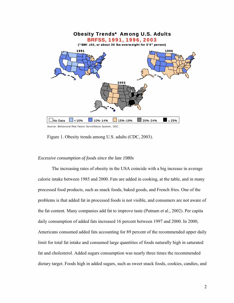
the obesity rate for adults rose from 12 percent to 18 percent (Nestle, 2002). In 2003,
according to the Centers for Disease Control and Prevention (CDC, 2003), 15 states had
obesity prevalence rates between 15 and 19 percent; 31 states were between 20 and 24
percent; and 4 states had rates greater than 25 percent. Figure 1 highlights this phenomenon
across the states between 1991 and 2003.
2
Source: Behavioral Risk Factor Surveillance System, CDC.
19961991
2003
Obesity Trends* Among U.S. AdultsBRFSS, 1991, 1996, 2003
No Data <10% 10%-14% 15%-19% 20%-24% ≥ 25%
(*BMI ≥30, or about 30 lbs overweight for 5’4” person)
Source: Behavioral Risk Factor Surveillance System, CDC.
199619911991
2003
Obesity Trends* Among U.S. AdultsBRFSS, 1991, 1996, 2003
No Data <10% 10%-14% 15%-19% 20%-24% ≥ 25%
(*BMI ≥30, or about 30 lbs overweight for 5’4” person)
Figure 1. Obesity trends among U.S. adults (CDC, 2003).
Excessive consumption of foods since the late 1980s
The increasing rates of obesity in the USA coincide with a big increase in average
calorie intake between 1985 and 2000. Fats are added in cooking, at the table, and in many
processed food products, such as snack foods, baked goods, and French fries. One of the
problems is that added fat in processed foods is not visible, and consumers are not aware of
the fat content. Many companies add fat to improve taste (Putnam et al., 2002). Per capita
daily consumption of added fats increased 16 percent between 1997 and 2000. In 2000,
Americans consumed added fats accounting for 89 percent of the recommended upper daily
limit for total fat intake and consumed large quantities of foods naturally high in saturated
fat and cholesterol. Added sugars consumption was nearly three times the recommended
dietary target. Foods high in added sugars, such as sweet snack foods, cookies, candies, and

3
cola drinks often supply calories but few nutrients. Average annual consumption of caloric
sweeteners grew by 22 percent between 1980-84 and 2000. Moreover, U.S. per capita fruit
consumption is low. American consumers eat too few fruits and vegetables and tend to eat
a limited variety of vegetables. Half of Americans ate less than 1 serving of fruit daily in
1994-96 and less than a quarter consumed 3 fruits servings a day, which is the number
recommended by the U.S. Department of Agriculture Food Guide Pyramid (Putnam et al.,
2002).
Obesity, a socioeconomic problem
The societal cost of obesity in the United States has become a socioeconomic
problem. Low income U.S. households spend a greater percentage of their annual budget
on food than those with higher incomes. Low income households buy lower cost items with
a high energy density, such as sweets and fats. Diets with added sugars and fats have
replaced whole grain diets. With more resources, people do not necessarily consume
healthier foods (Drewnowski, 2003).
Darmon et al. (2002) show that economic constraints contribute to unhealthy food
choices. They predict the food choices individuals take to reduce their food budgets while
maintaining diets similar to the average population diet. They model isoenergetic diets by
linear programming. Then, they introduce a cost constraint to assess the effect of cost on
the foods selection by the program. Among low socioeconomic groups (households with
low income and low education level), the results show that the proportion of energy by
meat, dairy products, vegetables, and fruits decreases, but the proportion by sweets, added
fats, and cereals increases. Thus, a cost constraint influences food selection and decreases
the nutrient densities of diets for low income consumers. According to their study,
4
economic measures could be efficient in improving the nutritional intake of low
socioeconomic populations. The study also shows that although nutrition knowledge plays
an important role, economic constraints influence behavior such as dietary habits.
The U.S. Government envisions new policies to combat obesity problems. The first
option is to promote better food choices through better education, especially at the
childhood level. The second one is to implement new tax and price policies. Today, in at
least 18 states, sales of sweet and fat foods, such as soft drinks, snack foods, and candy are
taxed. These taxes yield more than $1 billion per year (Nestle, 2002). The proposal is to
put taxes on such products and to use tax proceeds to support health promotion campaigns.
As changing prices influence purchase choices, one of the solutions is to decrease prices of
vegetables and fruits to stimulate the purchase of these items (Nestle, 2002).
Justification of the Study
Obesity and overweight are both social and economic problems. The U.S.
Department of Health and Human Services is worried about interwoven societal problems.
How can the obesity trends among the U.S. population be reduced? What would be the
leverage to achieve this goal?
The goal of this study is to use socio-demographic factors to explain food
consumption leading to overweight and obesity. Results from this study can be used to
develop fiscal and policy measures to reduce obesity. The study explores the question of
whether increasing prices of fat and sweet food products, by putting higher taxes on these
types of foods, is relevant to encourage people to allocate their resources toward the
purchase of healthier foods, such as vegetables, fruits, and whole grain?
5
Description of the Study
In this study, we develop a model of rational addiction in food consumption based
on the “Theory of Rational Addiction” of Becker and Murphy (1988). Rational people
decide what they consume on the basis of food price and income, knowing the future health
consequences of eating certain types of foods. People are potentially addicted to certain
foods if an increase in their past consumption of these foods leads to an increase in their
current consumption of these same foods. In this study, we use a framework suggested by
this model to analyze empirically consumption of certain types of foods by using food price
variables as instruments for food consumption. The Body Mass Index (BMI) is the
dependent variable, divided in three categories: normal (BMI<25 kg/m2), overweight
(25≤BMI<30 kg/m2), and obese (BMI≥30 kg/m2). Six groups of independent variables are
considered: 1) the price of calories consumed derived from prices of different food groups
identified as representative of sugar, carbohydrates, and fats which are recognized to
induce gain in weight when they are overconsumed; 2) household income; 3) age; 4)
gender; 5) education level (top grade level attained); and 6) race.
A limited dependent variable model is used to determine which attributes
(independent variables) impact BMI of overweight and obese individuals. Classifying the
BMI of individuals in categories is an advantage: the effect of each attribute on the BMI is
assumed to be different for consumers according to their BMI category. Marginal impacts
of the independent variables on the three BMI categories (dependent variables) are
determined.
Data from the National Center for Chronic Disease Prevention and Health
Promotion, extracted from the Behavioral Risk Factor Surveillance System (BRFSS), are
6
used for this study. The objective of the BRFSS is to collect data across states by a
telephone survey on preventive health practices and risk behaviors in the adult population.
In our study, data for four states and three years (1991, 1997, and 2002) are used to account
for the evolution of the BMI for the last decade. Monthly food prices data from the Annual
Summaries of the National Agricultural Statistics Service (United States Department of
Agriculture) are matched with the BRFSS survey data.
Study Objectives and Hypothesis
The specific objectives of this study are
1) To develop a model of rational addiction in food consumption
2) To determine the relationship between BMI and the selected food groups
3) To test the rational addiction model empirically and to estimate differential price
effects of addictive foods on normal, overweight, and obese people
As sugar is considered as an addictive food, the hypothesis tested in this study is that
lower sugar price significantly increases the Body Mass Index and the obesity rate among
the population.
Outline
Chapter 2 focuses on a literature review about trends of overweight and obesity in
the world and in the United States, and the addictive consumer behavior related to sugar.
Chapter 3 develops the theoretical model of rational addiction in food consumption. The
empirical model and data used in the analysis are presented in Chapter 4. Chapter 5 reports
and discusses the results. Chapter 6 presents the conclusion and provides suggestions for
policy considerations, limitations, and recommendations for further studies.

7
CHAPTER 2. LITERATURE REVIEW
Trends of BMI in the World and in the United States
Obesity was compared to an “epidemic” by the World Health Organization (WHO)
in 2000 in Geneva and recognized it as a “neglected public health problem” today in the
United States (American Obesity Association. “Obesity in the U.S.,” 2002). Overweight
and obesity result from an imbalance involving excessive calorie consumption and/or
inadequate physical activity. For each individual, body weight is the result of a
combination of genetic, metabolic, behavioral, environmental, cultural, and socioeconomic
influences. A person gains weight when he/she consumes more calories from food than the
body uses through its normal functions (Basal Metabolic Rate, BMR) and physical activity
(U.S. Department of Health and Human Services).
Trend of BMI in the world
More than 1 billion adults in the world are overweight, and approximately 300
million are obese. The WHO (2003) mentions “epidemic proportions” and deals with
“globesity.” The underlying shifts in society, such as modernization and urbanization, are
partially responsible for the rising prevalence of overweight and obesity.
In Africa and Asia, the BMI for adults is about 22-23 kg/m2. But in North America,
Europe, and in North African, Latin American, and Pacific Island countries, the BMI
reaches 25-27 kg/m2. In China and Japan, the current obesity level is less than 5 percent
(WHO, 2002). Nevertheless, in some big cities, the obesity prevalence is much higher and
can hit 20 percent. In economically advanced regions of developing countries, especially in
urban areas, the obesity rate has become equal to the rate reached by industrialized
countries (American Obesity Association. “Obesity – A Global Epidemic,” 2002).

8
In Europe, obesity rates have increased by 10 to 40 percent during the last 10 years
(American Obesity Association. “Obesity – A Global Epidemic,” 2002). Globally, among
children and adolescents, obesity rates increased in both developing and developed
countries. Moreover, the higher obesity rates were obtained with women and the higher
overweight rates with men. Note that under-nutrition1 and obesity co-exist in many
developing countries.
Trend of BMI in the United States
In the United States, 127 million adults are overweight; 60 million are considered as
obese; and 9 million are severely obese. Table 1 contains figures about the prevalence of
overweight, obesity, and severe obesity among American adults from 1976 to 2000
(American Obesity Association. “Obesity in the U.S.,” 2002). Between the end of the
1970s and the end of the 1990s, the prevalence of overweight people increased by 40
percent. During this same period, the obesity prevalence had more than doubled. Between
the end of the 1980s and the end of the 1990s, the severe obesity prevalence increased by
62 percent.
Table 1. Prevalence of overweight, obesity, and severe obesity among U.S. adults Overweight
(BMI>25) Obesity
(BMI>30) Severe Obesity
(BMI>40) 1999 to 2000 64.5 30.5 4.7 1988 to 1994 56.0 23.0 2.9 1976 to 1980 46.0 14.4 No data
Source: CDC, National Center for Health Statistics, National Health and Nutrition Examination Survey. Health, United States, 2002. Flegal et. al. JAMA. 2002;288:1723-7. NIH, National Heart, Lung, and Blood Institute, Clinical Guidelines on the Identification, Evaluation and Treatment of Overweight and Obesity in Adults, 1998. (American Obesity Association. “Obesity in the U.S.,” 2002). 1 Under-nutrition: a Body Mass Index less than 18.5.
9
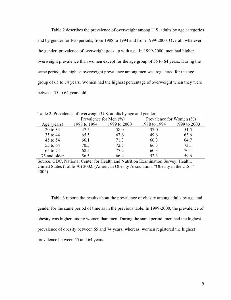
Table 2 describes the prevalence of overweight among U.S. adults by age categories
and by gender for two periods, from 1988 to 1994 and from 1999-2000. Overall, whatever
the gender, prevalence of overweight goes up with age. In 1999-2000, men had higher
overweight prevalence than women except for the age group of 55 to 64 years. During the
same period, the highest overweight prevalence among men was registered for the age
group of 65 to 74 years. Women had the highest percentage of overweight when they were
between 55 to 64 years old.
Table 2. Prevalence of overweight U.S. adults by age and gender Prevalence for Men (%) Prevalence for Women (%)
Age (years) 1988 to 1994 1999 to 2000 1988 to 1994 1999 to 2000 20 to 34 47.5 58.0 37.0 51.5 35 to 44 65.5 67.6 49.6 63.6 45 to 54 66.1 71.3 60.3 64.7 55 to 64 70.5 72.5 66.3 73.1 65 to 74 68.5 77.2 60.3 70.1
75 and older 56.5 66.4 52.3 59.6 Source: CDC, National Center for Health and Nutrition Examination Survey. Health, United States (Table 70) 2002. (American Obesity Association. “Obesity in the U.S.,” 2002).
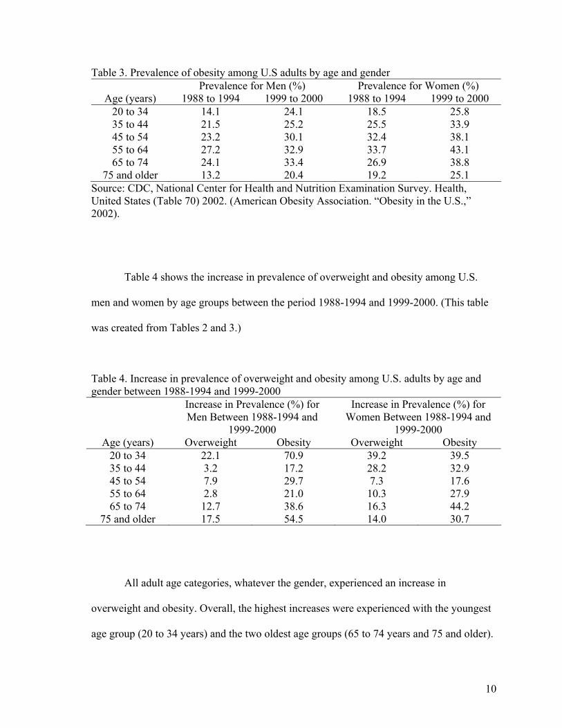
Table 3 reports the results about the prevalence of obesity among adults by age and
gender for the same period of time as in the previous table. In 1999-2000, the prevalence of
obesity was higher among women than men. During the same period, men had the highest
prevalence of obesity between 65 and 74 years; whereas, women registered the highest
prevalence between 55 and 64 years.
10
Table 3. Prevalence of obesity among U.S adults by age and gender Prevalence for Men (%) Prevalence for Women (%)
Age (years) 1988 to 1994 1999 to 2000 1988 to 1994 1999 to 2000 20 to 34 14.1 24.1 18.5 25.8 35 to 44 21.5 25.2 25.5 33.9 45 to 54 23.2 30.1 32.4 38.1 55 to 64 27.2 32.9 33.7 43.1 65 to 74 24.1 33.4 26.9 38.8
75 and older 13.2 20.4 19.2 25.1 Source: CDC, National Center for Health and Nutrition Examination Survey. Health, United States (Table 70) 2002. (American Obesity Association. “Obesity in the U.S.,” 2002).
Table 4 shows the increase in prevalence of overweight and obesity among U.S.
men and women by age groups between the period 1988-1994 and 1999-2000. (This table
was created from Tables 2 and 3.)
Table 4. Increase in prevalence of overweight and obesity among U.S. adults by age and gender between 1988-1994 and 1999-2000 Increase in Prevalence (%) for
Men Between 1988-1994 and 1999-2000
Increase in Prevalence (%) for Women Between 1988-1994 and
1999-2000 Age (years) Overweight Obesity Overweight Obesity
20 to 34 22.1 70.9 39.2 39.5 35 to 44 3.2 17.2 28.2 32.9 45 to 54 7.9 29.7 7.3 17.6 55 to 64 2.8 21.0 10.3 27.9 65 to 74 12.7 38.6 16.3 44.2
75 and older 17.5 54.5 14.0 30.7
All adult age categories, whatever the gender, experienced an increase in
overweight and obesity. Overall, the highest increases were experienced with the youngest
age group (20 to 34 years) and the two oldest age groups (65 to 74 years and 75 and older).
11
Among men, the overweight prevalence for people between 20 and 34 years old and for the
age group of 75 and older increased by 22.1 percent and by 17.5 percent respectively.
Concerning the male obesity prevalence, in one decade, the number of obese people aged
20 to 34 years increased by 70.9 percent. A high increase was also registered for men older
than 75 years. High increases in overweight were registered among young women between
20 and 34 years and 35 and 44 years, respectively 39.2 percent and 28.2 percent. Other age
groups had lower increases. Among women, all age groups had experienced high increases
in obesity prevalence. The lowest increase was recorded among women between 45 and 54
years old (17.6 percent) and the highest one between 65 and 74 years old (44.2 percent).
Overall, men had a higher prevalence in overweight than women (68.8 percent
versus 63.8 percent in 1999-2000). On the other hand, women had a higher prevalence in
obesity at the same date (34.1 percent versus 27.7 percent). In the last decade, men had the
highest increase in obesity (+38.7 percent); whereas, women had the highest rise in
overweight (+25.7 percent).
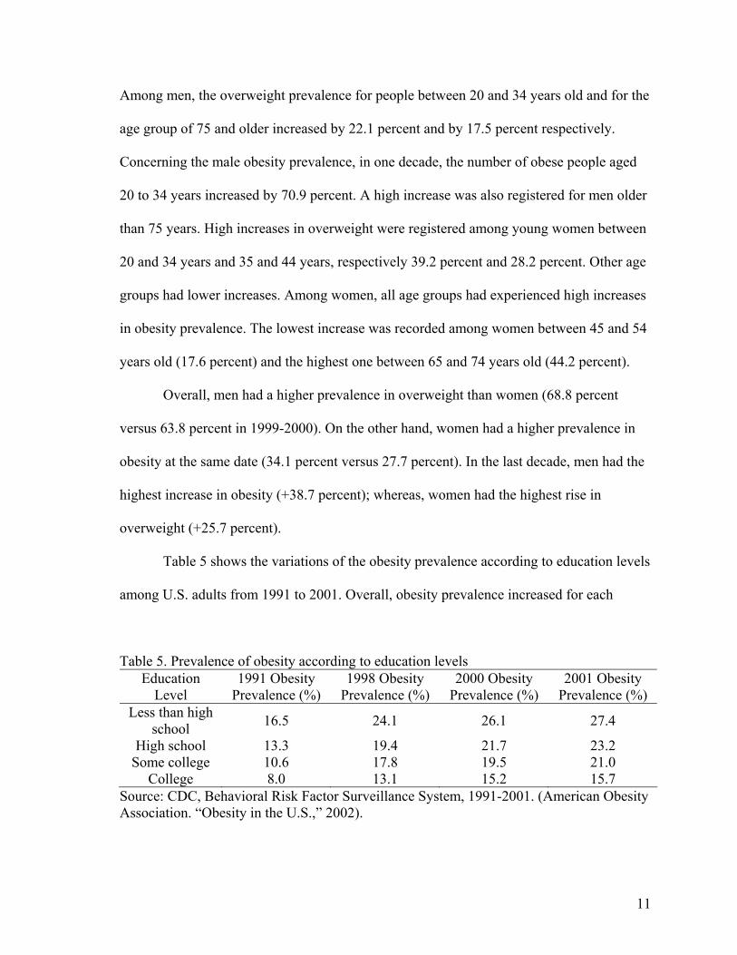
Table 5 shows the variations of the obesity prevalence according to education levels
among U.S. adults from 1991 to 2001. Overall, obesity prevalence increased for each
Table 5. Prevalence of obesity according to education levels Education
Level 1991 Obesity
Prevalence (%) 1998 Obesity
Prevalence (%) 2000 Obesity
Prevalence (%) 2001 Obesity
Prevalence (%) Less than high
school 16.5 24.1 26.1 27.4
High school 13.3 19.4 21.7 23.2 Some college 10.6 17.8 19.5 21.0
College 8.0 13.1 15.2 15.7 Source: CDC, Behavioral Risk Factor Surveillance System, 1991-2001. (American Obesity Association. “Obesity in the U.S.,” 2002).
12
education level in the last decade. However, people with higher education levels had lower
obesity rates than people with less education.
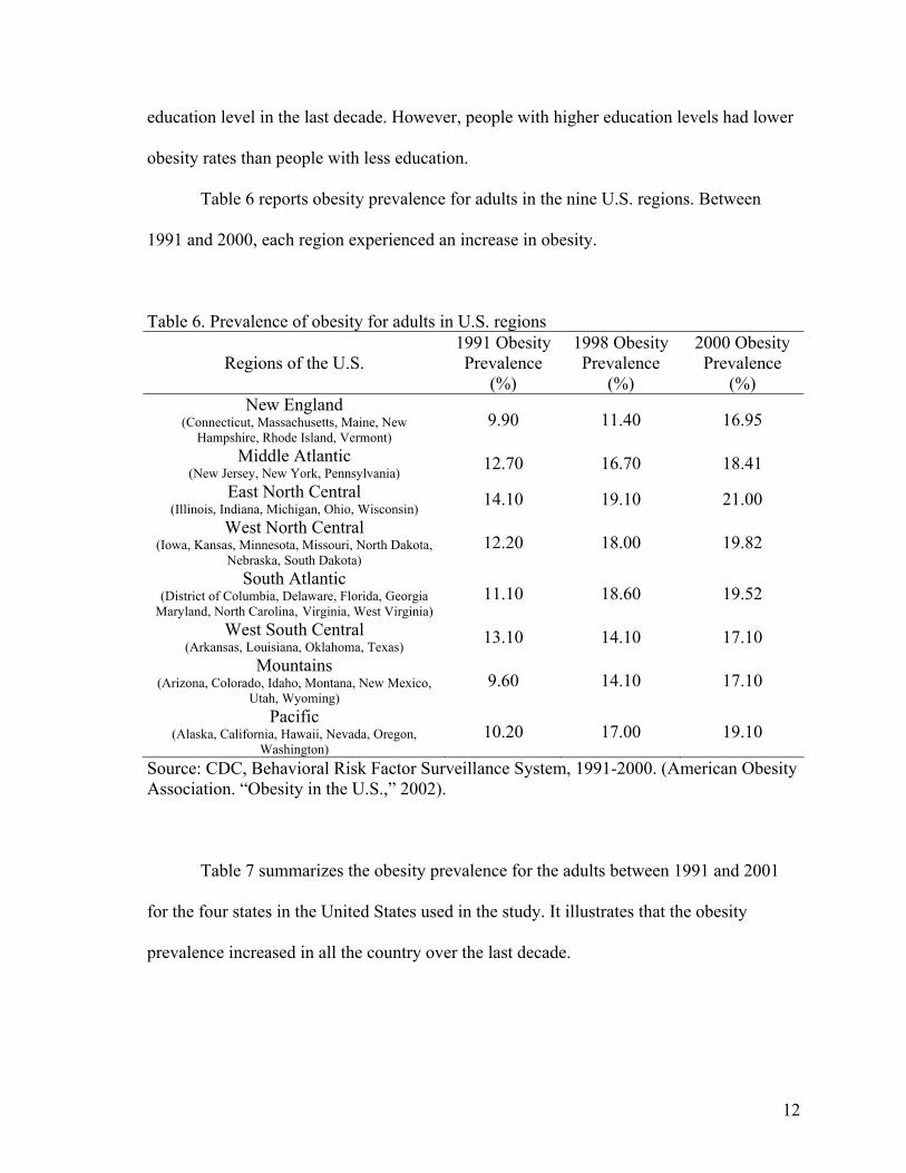
Table 6 reports obesity prevalence for adults in the nine U.S. regions. Between
1991 and 2000, each region experienced an increase in obesity.
Table 6. Prevalence of obesity for adults in U.S. regions
Regions of the U.S. 1991 Obesity Prevalence
(%)
1998 Obesity Prevalence
(%)
2000 Obesity Prevalence
(%) New England
(Connecticut, Massachusetts, Maine, New Hampshire, Rhode Island, Vermont)
9.90 11.40 16.95
Middle Atlantic (New Jersey, New York, Pennsylvania) 12.70 16.70 18.41
East North Central (Illinois, Indiana, Michigan, Ohio, Wisconsin) 14.10 19.10 21.00
West North Central (Iowa, Kansas, Minnesota, Missouri, North Dakota,
Nebraska, South Dakota) 12.20 18.00 19.82
South Atlantic (District of Columbia, Delaware, Florida, Georgia
Maryland, North Carolina, Virginia, West Virginia) 11.10 18.60 19.52
West South Central (Arkansas, Louisiana, Oklahoma, Texas) 13.10 14.10 17.10
Mountains (Arizona, Colorado, Idaho, Montana, New Mexico,
Utah, Wyoming) 9.60 14.10 17.10
Pacific (Alaska, California, Hawaii, Nevada, Oregon,
Washington) 10.20 17.00 19.10
Source: CDC, Behavioral Risk Factor Surveillance System, 1991-2000. (American Obesity Association. “Obesity in the U.S.,” 2002).
Table 7 summarizes the obesity prevalence for the adults between 1991 and 2001
for the four states in the United States used in the study. It illustrates that the obesity
prevalence increased in all the country over the last decade.

13
Table 7. Prevalence of obesity for U.S. adults in the four states used in the study between 1991 and 2001
U.S. states 1991 Obesity Prevalence (%)
1998 Obesity Prevalence (%)
2000 Obesity Prevalence (%)
2001 Obesity Prevalence (%)
California 10.0 16.8 19.2 20.9 Idaho 11.7 16.0 18.4 20.0
Michigan 15.2 20.7 21.8 24.4 Minnesota 10.6 15.7 16.8 19.2
Source: CDC, Behavioral Risk Factor Surveillance System, 1991-2001. (American Obesity Association. “Obesity in the U.S.,” 2002).
Does Eating Sugar Make People Obese?
According to the Reference Dietary Intakes, the Food Guide Pyramid, the Dietary
Guidelines for Americans, and the American Dietetic Association, all foods consumed in
moderation can fit into a healthful eating style. Many factors influence eating practices:
taste and food preferences, lifestyle, environment, concerns about nutrition and weight
control, and food product safety.
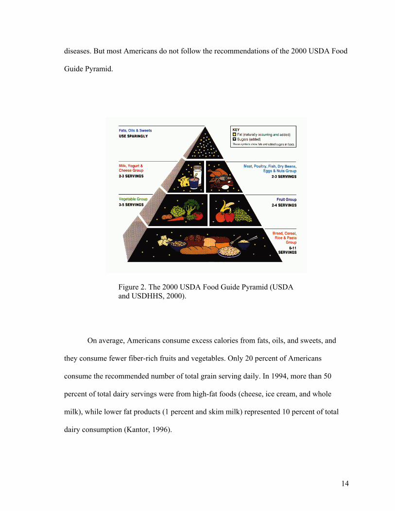
The 2000 USDA Food Guide Pyramid provides some information and
recommendations for the quantity and type of foods to eat from 5 major groups: 1) bread,
cereals, rice, and pasta; 2) vegetables; 3) fruits; 4) milk, yogurt, and cheese; 5) meat,
poultry, fish, dry beans, eggs, and nuts.
The pyramid (Figure 2) presents a range of recommended servings for each food
group for sample levels of energy intakes. The number of servings recommended for each
food group depends on an individual’s age, physiological status, and energy requirements.
Healthy diets, including vegetables, grains, and fruits, and low in fat, saturated fat, and
cholesterol, combined with moderate and regular physical activity, reduce the risk of
14
diseases. But most Americans do not follow the recommendations of the 2000 USDA Food
Guide Pyramid.
Figure 2. The 2000 USDA Food Guide Pyramid (USDA and USDHHS, 2000).
On average, Americans consume excess calories from fats, oils, and sweets, and
they consume fewer fiber-rich fruits and vegetables. Only 20 percent of Americans
consume the recommended number of total grain serving daily. In 1994, more than 50
percent of total dairy servings were from high-fat foods (cheese, ice cream, and whole
milk), while lower fat products (1 percent and skim milk) represented 10 percent of total
dairy consumption (Kantor, 1996).
15
A high-fat diet promotes the development of obesity with a direct relationship
between the amount of dietary fat and the degree of obesity. Golay and Bobbioni (1997)
indicate by animal studies that high-fat diets induce greater food intake and weight gain
than high-carbohydrate diets because of several factors, such as caloric density, satiety
properties, and post-absorptive processing. For instance, the satiating effects after meals
with a weak “fat/carbohydrate” ratio are greater than for meals with a higher ratio. The
overconsumption of energy as fat in obese patients would be due to eating a high-fat meal
when hunger is high. Thus, dietary fat induces overconsumption and weight gain because
of its high caloric density and its low satiety properties (Hill, 1999).
Preference for fat is a factor which must be taken into account for obesity. Some
research shows that obese people prefer the same concentration of sugar but higher
concentrations of fat than normal-weight people. Many popular sweet foods, such as
chocolate, ice cream, cookies, and cakes, contain fat. Moreover, it is demonstrated that
eating five to nine servings of fruits and vegetables daily reduces the incidence of several
diseases, such as heart diseases and high blood pressure (Hill, 1999). Fruits and vegetables
are sources of fiber. Fiber plays a role in regulating blood sugar, lowering blood cholesterol,
and also in controlling weight.
Newby et al. (2003) find that smaller gains in BMI and waist circumference are
associated with a consumption of diets high in vegetables, fruits, reduced-fat dairy, and
whole grains; and low in red and processed meat, fast food, and soda (diet low in glycemic
load). The greater gains are obtained with a consumption of diets high in meat and potatoes
and with a consumption of diets high in white bread, pizza, and fast food (food with a high
glycemic index value and low in fiber). The explanations are that fiber in vegetables, fruits,

16
and whole grains increases satiety and decreases insulin response, which decreases hunger
and energy intake. Moreover, vegetables, fruits, and whole grains are low in energy density
(Newby et al., 2003).
One of the explanations about the increasing rates of overweight or obesity in the
United States is recent eating habits with a sedentary lifestyle. Commonly, nutritionists
implicate consumption of snacks, fast foods, and soft drinks. It is true that Americans often
consume foods away-from-home. The problem is that these items contain usually more salt,
sugar, and fat. Overall, the percentage of household total expenditures dedicated to food
purchases decreases as income increases. According to Economic Research Service (ERS)
of the USDA, in 1998, 11.6 percent of Americans’ income is spent for food. Of this
percentage, 7.4 percent was for at-home food and 4.2 percent for away-from-home foods
(Putnam and Allhouse, 1999). Similarly, with easier access to new food technologies and to
processed foods, people tend to eat more daily meals, and consequently their caloric intake
increases (Culter et al., 2003). Moreover, overconsumption of sugar-sweetened beverages,
corn syrup, potatoes, and refined grains induce a higher risk of diabetes and heart diseases
(Drewnoswski et al., 2004).
In 2000, 77 percent of Americans thought that there were “good” and “bad” foods.
But this belief induces dichotomous thinking (Freeland-Graves and Nitzke, 2002). For
instance, the person feels certain self-control when he/she stays in the diet. But he/she may
lose control in a high risk situation (in front of an appealing food). Freeland-Graves and
Nitzke (2002) take the example of ice-cream. This food is considered as “bad”, but when
the dieter is attracted by this food, he/she may think, “I ate the ice-cream, I have blown my
diet. I’m going to finish the carton”. This thinking is related to addictive or compulsive

17
behaviours. The parallel is done with alcoholics when they break abstinence. When the
dieter breaks his/her objectives, he/she becomes weak and indulgent with himself/herself,
and the common idea is that a diet can start tomorrow.
The problem is that lower food prices induce people to consume more. Some people
have trouble controlling what they eat. Culter et al. (2003) discuss about “self-control
problems.” According to them, $30 to $50 billion is spent per year on diets. Overall, people
still overeat although they would like to lose weight.
The most important factor influencing food choice seems to be taste. The initial
factors influencing the taste are primarily genetic, metabolic, and physiological. Then,
individual experiences and eating behaviours play a role. Taste preference for sweetness is
inborn; whereas, taste preference for fat is learned in early childhood (Drewnowski, 1997).
A sweet taste has an attraction for many animals and for humans. Many studies
investigate food preference and diet-induced overeating, especially on laboratory rats. If
rats have the choice between foods with different compositions, they prefer high-fat and/or
high-sugar foods. Moreover, their total energy intake may rise by 20 to 40 percent. Rats
may become mildly or moderately obese in eating “supermarket” foods, such as cookies or
milk, with their standard chow (Sclafani, 2001). The hedonism phenomenon plays an
important role with the flavor stimuli on food selection and intake.
The combination of fat and sugars in foods are commonly preferred. For fat and
sugar appetites, some studies give explanations related to hormonal mechanisms, including
endogenous opiate peptides (endorphins) and binge eating. Other studies find that peak
hedonic rating is achieved with mixtures containing 20 percent fat and 8 percent sucrose.
This peak is obtained with products such as ice cream, sweetened cream cheese, and cake
18
frostings. The common point between these foods is that they contain milk, cream, and
sugar (Drewnowski, 1997).
Brain peptides or neurotransmitters may mediate the sensory pleasure response to
sweetness and fat. Endorphins play a role in food cravings, drug reward, and in the binge-
eating syndrome in obesity and bulimia nervosa. It is shown that preferences for sweet taste
are increased by opiate secretion. On the other hand, opiate antagonists reduce food intake
in declining taste preferences for sweet and high-fats foods. Parallels between binge-eating
and drug addiction can be done because these phenomena are both under opiate control and
imply loss of control and cravings. Appetites for sweets and opiate addictions are
associated. Eating ice cream and chocolate decreases the feeling of opiate lack
(Drewnowski, 1997).
Binge-types of foods are commonly ice cream, doughnuts, candy, cookies, popcorn,
milk, and sandwiches. They are rich in fat and sugar and consumed in large quantities
during a binge. According to clinical experiences, carbohydrates play the major role in
obesity and in binge-eating. When people are stressed, they tend to eat sweet snacks
because sugar increases endorphin production, which has a tranquilizing effect. Obese
people have stronger preference for sweet tastes than non-obese people. They usually have
an excess of carbohydrates in their daily diet (Fullerton et al., 1985).
Bray et al. (2004) suggest that consumption of high-fructose corn syrup (HFCS) in
beverages may play a role in the increase in obesity. In the United States, HFCS represents
more than 40 percent of caloric sweeteners added to foods and beverages. Moreover, it is
the only caloric sweetener used for soft drinks. Between 1970 and 1990, consumption of
HFCS rose more than 1,000 percent. The main reason is that HFCS is much cheaper than

19
sucrose (sugar) for manufacturers. HFCS is included in most soft drinks and fruit drinks,
canned fruits, flavoured yogurts and dairy desserts, many cereals, jellies, and in most baked
goods. This evolution is parallel to the increase of obesity. It is suggested that dietary
fructose may contribute to increased energy intake and may induce weight gain. Hence,
sweetened beverages may bring up caloric overconsumption. Nevertheless, many factors
induce excessive caloric intake, such as increased portion sizes, overconsumption of
sweetened beverages, high-fat foods, and diets high both in simple sugars such as sucrose
and in HFCS as a source of fructose.
In this context, the obvious question is the following: is there significant difference
between sucrose from traditional sugar (produced for instance from sugarbeets) and
fructose from the high fructose corn syrup? Apparently, there is no difference. Jacobson
(2004) suggests that even if soft drinks were still sweetened with sucrose, they would have
contributed just as much to overweight and obesity prevalence. Moreover, the body gets
almost similar amounts of glucose and fructose in consuming either HFCS or sucrose. In
the beverage industry, the fructose content of high-fructose corn syrup is only slightly
higher (5 percent) than the fructose content of sucrose. Overall, according to Saris (2003),
there is no significant change in metabolic response with an increasing use of HFCS. Price
is the only difference between sucrose and HFCS. Food companies gain 1 cent in
sweetening a 12-ounce can of soft drink with HFCS instead of sucrose. In other words, it is
not useful to differentiate foods sweetened with HFCS or sucrose. Moreover, it is
impossible to determine by how much the shift from sucrose to high fructose corn syrup
has contributed to the increasing consumption of soft drinks and in consequence to the
20
development of obesity (Bray et al., 2004). Finally, in this study, prices of sucrose and
HFCS are assumed to be positively correlated.
In summary of the literature cited, carbohydrates, and particularly sugars, are
implicated in the problem of overweight and obesity. Eating sugar leads to eating more,
and the combination of increasing consumption of carbohydrate-sweetened beverages and
foods with the decreasing physical activity contributes much to raise the risk of weight gain.
21
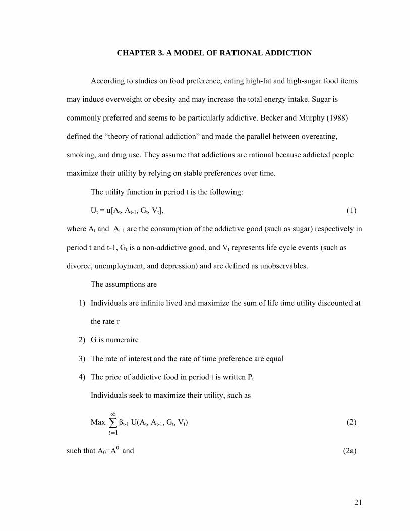
CHAPTER 3. A MODEL OF RATIONAL ADDICTION
According to studies on food preference, eating high-fat and high-sugar food items
may induce overweight or obesity and may increase the total energy intake. Sugar is
commonly preferred and seems to be particularly addictive. Becker and Murphy (1988)
defined the “theory of rational addiction” and made the parallel between overeating,
smoking, and drug use. They assume that addictions are rational because addicted people
maximize their utility by relying on stable preferences over time.
The utility function in period t is the following:
Ut = u[At, At-1, Gt, Vt], (1)
where At and At-1 are the consumption of the addictive good (such as sugar) respectively in
period t and t-1, Gt is a non-addictive good, and Vt represents life cycle events (such as
divorce, unemployment, and depression) and are defined as unobservables.
The assumptions are
1) Individuals are infinite lived and maximize the sum of life time utility discounted at
the rate r
2) G is numeraire
3) The rate of interest and the rate of time preference are equal
4) The price of addictive food in period t is written Pt
Individuals seek to maximize their utility, such as
Max ∑∞
=1tβt-1 U(At, At-1, Gt, Vt) (2)
such that A0=A0 and (2a)

22
W = ∑∞
=1tβt-1 (Gt + PtAt), (2b)
where β=1/(1+r), Pt is the price of foods in period t, and W is the present value of wealth.
Effects of addictive food’s consumption on earnings, on the present value of wealth, and on
the length of life are not taken into account. A0 is the initial condition for the consumer in
period 1 and measures the level of addictive food in the period prior to that under
consideration.
The first-order conditions are as follows:
Ug(At, At-1, Gt, Vt) = λ (3a)
U1(At, At-1, Gt, Vt) + βU2(At, At-1, Gt+1, Vt+1) = λ Pt. (3b)
Ug is the marginal utility of consumption in each period. The summation of U1, marginal
utility of current addictive food consumption, and U2, the discounted marginal effect of the
current consumption on the future utility, is equal to the current price multiplied by the
marginal utility of wealth, λ. U2 is negative with harmful, addictive food.
Since the marginal utility of wealth, λ, is constant over time, changes in the price of
the addictive food over time trace out marginal utility of wealth-constant demand curves
for G and A. If utility is considered as non separable, the demand curves depend on prices
in all periods through the effects of past and future prices on past and future consumption.
For instance, consider a utility function quadratic in Gt, At, and Vt. The first-order
conditions are as follows:
Ug + UggGt + UgAt + Uy2At-1 + UgvVt = λ (4a)
U1 + U1gGt + U11At + U12At-1 + U1vVt + ß(U2 + U2gGt+1 + U22At + U2vVt+1) = λPt. (4b)
Equation 4a can be solved for Gt in terms of λ and At:
23
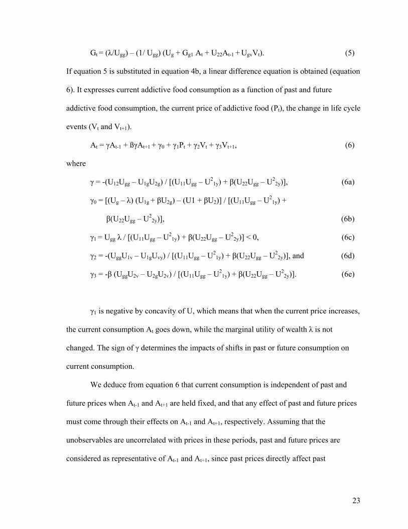
Gt = (λ/Ugg) – (1/ Ugg) (Ug + Gg1 At + U22At-1 + UgvVt). (5)
If equation 5 is substituted in equation 4b, a linear difference equation is obtained (equation
6). It expresses current addictive food consumption as a function of past and future
addictive food consumption, the current price of addictive food (Pt), the change in life cycle
events (Vt and Vt+1).
At = γAt-1 + ßγAt+1 + γ0 + γ1Pt + γ2Vt + γ3Vt+1, (6)
where
γ = -(U12Ugg – U1gU2g) / [(U11Ugg – U21y) + β(U22Ugg – U2
2y)], (6a)
γ0 = [(Ug – λ) (U1g + βU2g) – (U1 + βU2)] / [(U11Ugg – U21y) +
β(U22Ugg – U22y)], (6b)
γ1 = Ugg λ / [(U11Ugg – U21y) + β(U22Ugg – U2
2y)] < 0, (6c)
γ2 = -(UggU1v – U1gUvy) / [(U11Ugg – U21y) + β(U22Ugg – U2
2y)], and (6d)
γ3 = -β (UggU2v – U2gU2v) / [(U11Ugg – U21y) + β(U22Ugg – U2
2y)]. (6e)
γ1 is negative by concavity of U, which means that when the current price increases,
the current consumption At goes down, while the marginal utility of wealth λ is not
changed. The sign of γ determines the impacts of shifts in past or future consumption on
current consumption.
We deduce from equation 6 that current consumption is independent of past and
future prices when At-1 and At+1 are held fixed, and that any effect of past and future prices
must come through their effects on At-1 and At+1, respectively. Assuming that the
unobservables are uncorrelated with prices in these periods, past and future prices are
considered as representative of At-1 and At+1, since past prices directly affect past
24
consumption, and future prices have a direct impact on future consumption. Thus, γ and γ1
are estimated empirically by using past and future price variables as instruments for past
and future consumption.
Lower past or future food prices are assumed to increase past or future consumption.
Thus, if γ is positive, lower past or future food prices will increase current consumption.
On the contrary, if γ is negative, increases in past or future consumption would bring down
current consumption. Past and current consumption are complement only if γ is positive,
and the addiction is stronger when γ is higher. This phenomenon is called reinforcement: it
means that people with a high past consumption of goods have greater desire for present
consumption. The greater the reinforcement from past consumption, the more addictive the
food. In other words, a good is addictive if γ > 0 and when γ is larger, the degree of
addiction is higher. The second phenomenon is called tolerance, which means that when
past consumption is greater, the current utility is lower because of the harmful effects of
addictive goods.
Two categories of consumers are defined. The “myopic utility maximizers” do not
take into account the future consequences of their current consumption; whereas, the
“rational utility maximizers” do (Becker et al., 1990). Among rational addicts, people who
discount the future heavily are more likely to be addicted because they are not worried
about the harmful consequences. In addition, the addiction is greater when the effects of
past consumption depreciate more rapidly. In this case, current consumption does not
decrease the future utility much.
Models of myopic and rational addiction are different, and their results are also
different. Myopic individuals do not consider the future consequences of current

25
consumption and do not consider a potential change in their future utility. For them, current
consumption depends on current price, the marginal utility of wealth, lagged consumption,
and current events. Thus, they do not respond to future price changes as rational individuals
do. For instance, if the future price changes, it will not have any impact on the current
consumption of the addictive food for myopic consumers.
In this model, the first-order conditions are
Ug + UggGt + UgAt + Ug2At-1 + UgvVt = λ (8a)
U1 + U1gGt + U11At + U12At-1 + U1vVt = λPt (8b)
The term of the future impact ßU2 does not appear in equation 8b because current
consumption, in this case, is not related to future consumption At+1 and future life events
Vt+1.
It is important to notice that the model of rational addiction and the model of
myopic addiction, by their different structures, give different results about responses to
future changes. The study focuses on the model of rational addiction in food consumption.
From the model of rational addiction developed for food consumption, an empirical
test is performed (Chapter 4) using past and future prices (Pt-1 and Pt+1) as instruments
representative of past and future consumption (At-1 and At+1) of the addictive foods. The
objective of the study is to know how overweight and obese people respond to a change of
prices on sweet food products in order to help to develop an effective policy using taxes.

26
CHAPTER 4. EMPIRICAL METHODS AND PROCEDURES
Equation (6) derived from the utility function (equation 1) is used as the basis of the
empirical model in this study. Addictive food consumption in period, t, is defined as a
function of addictive food consumption in period, t-1, and in period, t+1, the current price
of addictive food, Pt, and the unobservables Vt and Vt+1. This estimation induces biased
estimates because unobservable errors that affect utility in each period are likely to be
serially correlated. Positive serial correlation in the unobserved effects erroneously implies
that past and future consumptions have a positive impact on current consumption, even
when the true value γ is equal to zero. Nevertheless, this problem can be avoided thanks to
developments by Hansen (1982). Equation (6) involves that current consumption is
independent of past and future prices when At-1 and At+1 are held fixed. This equation also
implies that any impacts of past and future prices are reflected by their impacts on At-1 and
At+1. Moreover, the unobservables are assumed to be uncorrelated with prices in these
periods. Thus, past and future prices can be used to approach past and future consumption.
The empirical strategy is to estimate γ and γ1 from equation 6 by using Pt-1 and Pt+1 as
instruments for At-1 and At+1. As data for current consumption of food are not available
from the BRFSS survey, the current consumption is empirically approached by the
individual body mass index. It is assumed that when the food consumption increases, the
BMI increases, and vice versa.
To test the rational addiction model empirically and to estimate differential price
effects of addictive foods on people, the multinomial logit model is used. This study
assumes that individuals can fall into three BMI categories: normal, overweight, and obese.
In this model, the probability of falling in one of the three BMI categories is a function of

27
past, current, and future prices of foods (sugarbeet, potato, and whole milk). Some
socioeconomic variables and demographic variables are also taken into account, such as
gender, age, household income, grade, and race.
The multinomial logit model is used because the dependent variable, the BMI
category, is qualitative in nature, and it is classified in more than two alternatives. The
marginal impacts of the independent variables, such as food prices, gender, age, income,
grade, and race on the three BMI categories can be determined.
The three advantages of multinomial logit model are the following (Kennedy, 1996):
1) its computational ease; 2) the expression of the probability that a consumer selects a
given alternative is easy to obtain; and 3) a likelihood function can be determined and
maximized straightforward.
The probability that a consumer will fall in a given BMI category is estimated as a
function of food prices and consumer attributes. The assumptions required by the model are
1) We assume that people can choose to increase their BMI by overeating addictive
foods, especially when prices of these foods are low
2) εij is a random independent variable with a Weilbull distribution, and the
distribution of the differences between εij is logistic (Domencich and McFadden,
1975)
It is assumed that the BMI category “normal” is the base category and is chosen
outside of the modeling framework. Therefore, the probability of selecting or falling in the
base category is undetermined in the present choice set. Nevertheless, in normalizing the
coefficients for “normal” to zero, the problem disappears (Amemiya and Nold, 1975).
Maximum likelihood is utilized to estimate the coefficients for the other “overweight” and
28
“obese” categories. The probability of the jth individual adopting ith BMI category can be
calculated as (Greene, 1995):
Probij = ∑i
Xji'
iXj'
ee
β
β
(12)
To measure the effects of economic and demographic factors on the choice of BMI
category by individuals, a single equation multinomial logit model estimated by maximum
likelihood is used.
The marginal effects of price impacts and of the other socioeconomic variables can
also be estimated. In the discrete choice model, the effect of a change in attribute m (such
as prices, income, etc.) of the alternative j on the probability that the individual would
choose alternative k (where k may or may not equal j) is (Greene, 1995):
)(mjk∂ = ∂ Prob[yi=k]/∂ xij(m) = [1(j=k) – PjPk] mβ (13)
where Pj and Pk are the sample proportions of observations that make choices j and k
respectively and, mβ is the set of parameters which reflects the changes in X on the
probability.
It is essential to evaluate the differential price impacts on BMI to show that some
food pricing strategies could be employed in order to decrease BMI and, therefore decrease
the obesity prevalence. It is also interesting to determine which socioeconomic factors must
be considered to create some policies for the same goal.
The set of coefficients and marginal effects from the multinomial logit model are
estimated by the LIMDEP econometrics software package (Nlogit version 3.0).

29
CHAPTER 5. EMPIRICAL RESULTS AND DISCUSSIONS
Data and Estimation Procedures
Three years of BRFSS survey data are used: 1991, 1997, and 2002. They are
considered as period t. To this data set, prices for three different food commodities are
added. Food commodities include sugarbeets for sugar or sweetener category, potatoes for
carbohydrates, and whole milk for fat. State- and month-specific prices come from the
USDA. All price measures are deflated to 1989 dollar price to obtain real prices.
States for which price data are incomplete are deleted. Consequently, data for four
states are kept: California, Idaho, Minnesota, and Michigan. These represent three different
regions in the United States according to the climate and life-style: California for the West
Coast (Pacific), Minnesota and Michigan for the Upper Midwest, and Idaho for the Rocky
Mountains. The data set is representative of three major markets among five in the United
States. There is no gap in the state-specific price series for these four states. t-1 prices are
compiled for the years 1990, 1996, and 2001, and t+1 prices are compiled for the years
1992, 1998, and 2003.
In the data set, there are 45,440 observations (from the four states over three years).
State-specific demographic variables and BMI measures are available for the years of 1991,
1997, and 2002 and come directly from the survey. The analysis uses twenty-three
explanatory variables. Among these variables, ten variables are continuous variables and
represent age and food prices (historical, current, and future); two variables are discrete and
represent the income and education level (grade); and eleven are dummy variables for
gender, trends (time), regions, and races. The basic data used in the multinomial logit

30
model are presented in Table 8. This table reports variable definitions, means, and standard
deviations of the variables (data for four states and for the years 1991, 1997, and 2002).
Table 8. Descriptive statistics of data
Variable Name Variable Description Mean Standard Deviation
CURRENTS Current price of sugarbeet ($/ton) 38.95 1.75 CURRENTP Current price of potato ($/ton) 7.62 4.04 CURRENTM Current price of milk ($/ton) 12.18 1.06 HISTSUGA Historical price of sugarbeet ($/ton) 40.96 4.05 HISTPOTA Historical price of potato ($/cwt) 7.71 3.17 HISTMILK Historical price of milk ($/cwt) 13.91 1.39 FUTURESU Future price of sugarbeet ($/ton) 38.95 3.52 FUTUREPO Future price of potato ($/cwt) 7.31 3.39 FUTUREMI Future price of milk ($/cwt) 13.2 2.01 AGE Age of survey participants 46.65 17.64 INCOME Household income
1=less than $10,000 2=$10,000 to less than $15,000 3=$15,000 to less than $20,000 4=$20,000 to less than $25,000 5=$25,000 to less than $35,000 6=$35,000 to less than $50,000 7=$50,000 to less than $75,000 8=$75,000 or more 77=Don't know/Not sure 99=Refused
GRADE Highest grade or year of school completed 1=Eight grade or less 2=Some high school 3=High school grad. or GED cert. 4=Some technical school 5=Technical school graduate 6=Some college '7=College graduate 8=Post grad or professional degree 9=Refused
SEX Dummy for gender 1=Male 0=Female
DY97 Dummy for the year 1997 1=Year 1997 0=Otherwise

31
Table 8. (continued) Variable Name Variable Description Mean Standard
Deviation DY02 Dummy for the year 2002
1=Year 2002 0=Otherwise
DR1 Dummy for California 1=California 0=Otherwise
DR2 Dummy for Idaho 1=Idaho 0=Otherwise
DR4 Dummy for Minnesota 1=Minnesota 0=Otherwise
RBLACK Race:Black 1=Black 0=Otherwise
RASIAN Race: Asian or Pacific Islander 1=Asian or Pacific Islander 0=Otherwise
RINDIAN Race: American Indian or Alaska Native 1=American Indian or Alaska Native 0=Otherwise
ROTHER Race: Other 1=Other 0=Otherwise
DHISP Hispanic origin 1=Hispanic origin 0=Otherwise
In the BRFSS survey, only adults, defined as individuals with an age equal or
greater than 18 years, are interviewed. The average age of the sample used for the analysis
in this paper is 46.65 years, and the standard deviation is 17.64 years. The data set is
composed of 43.32 percent of men and 56.68 percent of women; whereas, for the United
States, the estimates for gender in 2004 are 49.22 percent of men and 50.78 percent of
32
women (Population Division, U.S. Census Bureau, 2005). Women are more interviewed
than men by the BRFSS.
Empirical Results
The number of individuals interviewed in 1991, 1997, and 2002 are 10,388, 16,029,
and 19,023 respectively for the four states. In this sample, 46.1 percent of the individuals
are classified as normal weight (BMI<25), 35.8 percent as overweight (25<BMI<30), and
18.1 percent as obese (BMI>30) according to their BMI.
The goal of the study is to determine which category of individuals, according to
their BMI, is more responsive to change in price of addictive foods. In the model of
rational addiction, the main implication is that addictive food consumption decisions are
linked over time. Indeed, current consumption is affected by both past and future
consumption. Past and future prices of addictive food affect directly past and future
consumption of this commodity and affect indirectly its current consumption when current
prices are held constant.
Three goodness of fit measures evaluate the overall fit of the model. This is due to
the type of model employed. Multinomial logit model has more than one goodness of fit
measure. It differs from the least square models, which have a single goodness of fit
measure.
Three goodness of fit measures are used in this study and are as follows:
1) McFadden R2 is defined as R2 = 1 – LΩ /Lφ, where LΩ is the unrestricted
maximum log-likelihood, and Lφ is the restricted maximum log-likelihood (slope
coefficients equal to zero)
33
2) The likelihood ratio test is calculated as 2(LΩ - Lφ) and is distributed as a χ²
random variable
3) The third goodness of fit measure is the percentage of correct predictions
These three measures, together, indicate the explanatory power’s level of the model.
The estimated value of the McFadden R2 is 13.12 percent. The explanatory
variables explain a significant portion of the variation in each variable on BMI categories.
The estimated chi-square test statistic is equal to 12,327.04 with 44 degrees of freedom,
and it is significant at 1 percent level. The percentage of correct predictions is equal to
90.94. The three measures of fit together indicate that the explanatory power of the model
is good. Moreover, a choice-based sampling is used to ensure the robustness of the model.
Thus, the estimation errors are minimized, but the coefficients are not affected.
To evaluate the significance of a variable, the p-value is used. The p-value is
determined when the standard normal probability of N[0,1] is greater or equal to the ratio
of the estimated variable to the estimated standard error of the variable (Greene, 1990). To
interpret the results, a 5 percent level of significance is chosen.
As the model is a multinomial logit, two sets of coefficients are mentioned: one for
“overweight” BMI category and one for “obese” BMI category. Whatever the set, most of
the coefficients are significant at 5 percent. Table 9 shows the estimated results. At 5
percent level of significance, higher current prices of sugar significantly decrease the
probability of being overweight and obese. At the same level of significance, future prices
of sugar significantly decrease the probability of being overweight, but they do not affect
the probability of being obese. According to the theory of rational addiction, people
consider the future. Knowing that the future sugar price will increase, addicted people such

34
as overweight people reduce their current consumption of sugar. Nevertheless, obese
people do not change their behavior if they perceive an increase in future prices of sugar.
Table 9. Results of Multinomial Logit Model Variable Coefficient Standard Error P[|Z|>z] Mean of X Characteristics in numerator of Prob[Y = overweight] CURRENTS -.07680001 .01080260 .0000 38.9491915 CURRENTP .04528994 .00632349 .0000 7.61806756 CURRENTM -.15255329 .01541028 .0000 12.1823059 HISTSUGA .01070024 .00963436 .2667 40.9633321 HISTPOTA -.06424005 .00663573 .0000 7.70904137 HISTMILK -.20540939 .01218226 .0000 13.9051664 FUTURESU -.01154373 .00474701 .0150 38.9475040 FUTUREPO .04361099 .00782818 .0000 7.31170401 FUTUREMI .57064080 .00919774 .0000 13.2036466 AGE .01371975 .00066510 .0000 46.6506162 INCOME -.00301098 .00057399 .0000 10.6086048 DSEX -.91287802 .02271410 .0000 .56683539 GRADE -.06795582 .00799855 .0000 4.76170775 DY97 -.65729332 .04267503 .0000 .35275088 DY02 .74438978 .06145698 .0000 .41863996 DR1 -.25700066 .06498955 .0001 .24282570 DR2 .26278263 .06789775 .0001 .24991197 DR4 -.03647870 .06363508 .5665 .27451585 RBLACK .31481508 .05589249 .0000 .04612676 RASIAN -.55477871 .08706321 .0000 .01828785 RINDIAN .21817161 .11222424 .0519 .01100352 ROTHER .08167952 .09030770 .3658 .01762764 DHISP .20056348 .04636514 .0000 .07185299 Characteristics in numerator of Prob[Y = obese] CURRENTS -.10144671 .01498595 .0000 38.9491915 CURRENTP .09746130 .00832766 .0000 7.61806756 CURRENTM -.34685136 .02045973 .0000 12.1823059 HISTSUGA .01550283 .01376143 .2599 40.9633321 HISTPOTA -.14303207 .00921846 .0000 7.70904137 HISTMILK -.41522533 .01618589 .0000 13.9051664 FUTURESU -.00982464 .00610750 .1077 38.9475040 FUTUREPO .08373276 .00974071 .0000 7.31170401 FUTUREMI .99200330 .01417189 .0000 13.2036466 AGE .00975946 .00082204 .0000 46.6506162 INCOME -.00652733 .00077843 .0000 10.6086048 DSEX -.45742857 .03012516 .0000 .56683539 GRADE -.16756340 .01102296 .0000 4.76170775 DY97 -1.28613944 .05599277 .0000 .35275088 DY02 1.43462536 .08817164 .0000 .41863996 DR1 -.73003552 .08531408 .0000 .24282570 DR2 .09243341 .08620950 .2836 .24991197 DR4 -.41096176 .08322180 .0000 .27451585 RBLACK .65952757 .06653430 .0000 .04612676 RASIAN -1.33054840 .14795942 .0000 .01828785 RINDIAN .55100566 .12989077 .0000 .01100352 ROTHER .22196769 .11035116 .0443 .01762764 DHISP .25710376 .05608637 .0000 .07185299
Obese people might be too addicted to sweet foods to reduce their consumption of
sweets. The other problem is that, in consuming sweet foods, people feel immediate
gratification, but the harmful consequences occur only in the future (Culter et al., 2003).
35
The effect of historical prices of sugar on the probability of falling in the “overweight” or
“obese” category is not significant.
In addition, the impact of current and future prices for potatoes (the proxy for
carbohydrates) on the BMI is significant and positive. According to the medical literature,
people addicted to sugar tend to eat more foods with high fat content and more
carbohydrates. Thus, even if current or future prices of potatoes increase, people will
continue consuming carbohydrates, and they may consume higher quantities due to their
addiction to sugar. For overweight and obese consumers, the impact of historical prices for
potatoes is negative. It seems that higher historical prices for this food will be more likely
to induce people to decrease the consumption of potatoes and to decrease the probability of
being overweight or obese. One reason for this phenomenon is that potatoes are not an
addictive food.
Current and historical prices of milk, representing fats, significantly decrease the
probability of adopting each of the BMI categories (“overweight” and “obese”) and vice
versa. However, if the future price of milk goes up, it is more likely that people will move
to BMI categories other than the “normal” category.
Some demographic variables are analyzed, such as age, household income, and
education level. The prevalence of overweight and obese adults goes up with age whatever
the gender: as people age, they become more likely to be overweight or obese. As the
household income rises, people are more likely to be less overweight and less obese. With
higher income, people can afford a variety of healthy foods, such as fruits and vegetables.
The results show that, with a higher education level, people are less likely to have a BMI
classified as overweight or obese. This result was expected because we suppose that

36
individuals with better education receive more information about nutrition and are more
aware of what a good diet should be. Moreover, with more disposable income, they can
afford more quality foods.
Finally, in the last set of variables, some binary dummy variables are used. They
provide information about trend (time), gender, races, and regions. The interpretation of the
coefficients from these dummies is done relative to the omitted dummy for each category
of variables.
Compared to 1991, the BMI trend in 2002 is significantly positive at 5 percent level
for “overweight” and “obese” categories. Indeed, CDC statistical results show a big
increase in overweight and in obesity in the United States between the beginning of 1990s
and now. The significant and negative estimate obtained for the year 1997 is unexpected.
This result could be explained by the fact that, between 1991 and 1997, the obesity rates for
the four given states did not increase much compared to the national obesity trend.
Concerning gender, men are less likely to be obese. This result corresponds to the literature
and CDC statistics. Nevertheless, it appears that men are less likely to be overweight,
which is belied by the CDC statistics. One explanation might be that the sample used for
the analysis is reduced and is not representative enough for the variable “gender”. Indeed,
more women than men were interviewed in the survey. Concerning races, the omitted
dummy is white individuals. All the interpretations are done relative to white individuals.
The results show that all the races, such as Blacks, American Indians, and Hispanics are
more likely to have overweight and obese people than the white race. The only exception is
represented by the Asians. Compared to white people, they may have significantly lower
BMI. Note that these results are not surprising.
37
The estimated coefficients of the regional dummies are interpreted relative to
Michigan. Individuals living in California are more likely to have a lower BMI than
Michigan because of the high percentage of Asians in this state (10.9 percent versus 1.8
percent)2, and the lower percentage of Blacks also (6.7 percent versus 14.2 percent)
contribute to these results. In addition, California residents are recognized as the healthiest
eaters in the United States. These people consume more salads, fresh eggs and yogurt,
bottled water, and wine (Nielsen, 2002). According to the U.S. Census Bureau, in San
Francisco, more than 94,000 people walk to get to work-at least twice as many per capita as
in any other city. San Francisco has many fitness centers, and a quarter of the Bay City’s
fitness facilities is constituted by yoga studios; whereas, Detroit has few fitness centers-
only about 1 for every 69,000 people (Horn, 2002). In Idaho, people are more likely to be
overweight than people living in Michigan. The reason could be that in Idaho there are
more people with Hispanic origin than in Michigan (7.9 percent versus 3.3 percent), and as
we have seen before, Hispanics are more likely to have a higher BMI compared to Whites.
Idaho is not significantly different from Michigan for the “obese” category. In addition,
Minnesota is not significantly different from Michigan for the “overweight” category, but
people from this state are less likely to be obese than people in Michigan. Michigan is more
industrial than Minnesota, and the population is composed by 14.2 percent of Blacks versus
3.5 percent in Minnesota. As previously, black people are more likely to be overweight and
obese compared to white people.
Marginal Impacts Analysis
2 Source: 2000 resident census population.

38
To understand how each independent variable impacts the results of the model, the
marginal probability of the variable must be determined. Table 10 reports the marginal
impacts of variables averaged over individuals on the probability to be classified as
“normal”, “overweight,” and “obese” according to the BMI. The entire results of the
marginal impacts are included as Appendix A.
Table 10. Summary of marginal effects Variable Y=Normal Y=Overweight Y=Obese CURRENTS .0166 -.0091 -.0075 CURRENTP -.0119 .0026 .0093 CURRENTM .0411 -.0075 -.0336 HISTSUGA -.0024 .0012 .0012 HISTPOTA .0171 -.0034 -.0137 HISTMILK .0524 -.0139 -.0385 FUTURESU .0022 -.0018 -.0004 FUTUREPO -.0109 .0033 .0076 FUTUREMI -.1366 .0503 .0863 AGE -.0025 .0022 .0003 INCOME .0008 -.0002 -.0006 DSEX .1550 -.1623 .0073 GRADE .0190 -.0024 -.0166 DY97 .1654 -.0475 -.1179 DY02 -.1861 .0554 .1307 DR1 .0774 -.0021 -.0753 DR2 -.0424 .0496 -.0072 DR4 .0283 .0220 -.0502 RBLACK -.0817 .0196 .0621 RASIAN .1534 -.0224 -.1310 RINDIAN -.0619 .0068 .0551 ROTHER -.0240 .0014 .0226 DHISP -.0429 .0243 .0185
Increasing the current price of sugar by one percent decreases the probability of
being in the “overweight” category by 0.91 percent, decreases the probability of being in
the “obese” category by 0.75 percent, and increases the likelihood of being in the “normal”
BMI category by 1.66 percent. Whatever the BMI category, marginal effects of historical
prices of sugar are not significant. People classified as “normal” and “overweight”

39
significantly respond to change in future prices of sugar. If future prices of sugar rise by
one percent, the likelihood of being in the “normal” BMI category goes up by 0.22 percent,
and the likelihood of being in the “overweight” category goes down by 0.18 percent, at 5
percent significance level. On the other hand, obese people do not significantly respond to
shifts in future prices of sugar. This lack of response may find its origin in the higher level
of addiction in sugar for obese people. As these individuals are highly addicted to sweet
foods, the future does not seem important to them. According to this analysis, obese people
do not change their consumption of sugar even if prices of sugar in the future increase. For
overweight and obese individuals, one percent higher current and future prices of potato
significantly increase the BMI.
On the other hand, a rise in historical prices of potatoes induces a decrease in the
probability of being in the “overweight” and “obese” categories by respectively 0.34
percent and 1.37 percent. Opposite results are found for individuals who are neither
overweight nor obese. Concerning whole milk, an increase by one percent in its historical
and current prices decreases the probability of being in the “overweight” and “obese”
categories; whereas, the same increase in future price for this commodity causes this
probability to increase. Results for individuals in the “normal” category are opposite.
With the age, the probability of being in the “normal” category decreases by 0.25
percent, and the probability to move to “overweight” and “obese” categories increases
respectively by 0.22 percent and 0.03 percent. The marginal effect of income is significant
and decreases the probability of higher BMI for overweight and obese individuals,
respectively by 0.02 percent and 0.06 percent. These effects are not really important
because Americans spend less than 10 percent of their income on food (Nestle, 2002).
40
Likewise, the marginal effect of education level decreases the probability of being in the
“overweight” and “obese” categories, respectively by 0.24 percent and 1.66 percent. These
higher figures show that education may be an essential policy variable to decrease the
prevalence of overweight and obesity.
Among the regions, when the marginal effects are significant at 5 percent level,
they are important. In this way, compared to Michigan, living in Idaho induces an increase
in the probability of being overweight by 4.96 percent. Marginal effects of regions such as
California and Minnesota on the probability of being overweight compared to Michigan are
not significant at 5 percent level. Likewise, the marginal effect of Idaho on the probability
of being obese compared to Michigan is also not significant for the same level.
Nevertheless, the marginal effects of living in California and in Minnesota decrease the
probability of being obese by 7.53 percent and 5.02 percent respectively, compared to
Michigan.
41
CHAPTER 6. CONCLUSIONS
Brief summaries are presented in this chapter about the problem addressed, the
objectives, the methodology, and the results. Finally, limitations of this study and
implications for further studies are stated.
Summary of Problem
In the United States, obesity is identified by the authorities now as the most
important public health concern. Moreover, it has become a socioeconomic problem due to
the cost to society. Approximately two-thirds of all deaths in the United States per year are
blamed on diet-related chronic diseases attributable to excess of weight. It costs the country
hundreds of billions of dollars annually in medical care and lost productivity (Finkelstein et
al., 2004). To bring down the obesity rate among the population, the U.S. Department of
Health and Human Services seeks a leverage as solution.
Some new policies are envisioned. The leverage would be to implement new tax
and price policies on some types of foods considered as harmful for health.
Summary of Objectives
The main objective of this study was to determine which economic factors affect
the increase in obesity in the United States. A theory of rational addiction adapted to food
consumption has been developed and has been tested by multinomial logit model. It was
used to predict how people, according to their body mass index, would respond to price
changes of “addictive” foods. The impacts of prices on people who were neither
overweight nor obese, on overweight people, and on obese people were determined. This
study will help policy makers quantify the marginal effects of food prices on the
probability of people being in one of the three categories of BMI.

42
Summary of Methodology
According to the medical literature, sugar is an addictive food. Thus, eating large
quantities of sugar is compared to an addictive behavior. This study developed a model of
rational addiction in food consumption based on the “Theory of Rational Addiction” of
Becker and Murphy (1988). The model was tested empirically using the multinomial logit
model. The population was divided into three categories according to the body mass index
to specify the differential responses to price of each group. In this model, the probability of
being in one of the three BMI categories (“normal,” “overweight,” and “obese”) was a
function of past, current, and future prices of foods and a function of several
socioeconomic and demographic variables.
Summary of Results
To evaluate the effectiveness of a potential “fat” tax policy, it is necessary
beforehand to determine which economic factors have impacts on people and, more
particularly, on which categories (“normal,” “overweight,” and/or “obese”). The
application of the multinomial logit model to our sample gave interesting results.
At a 5 percent level of significance, while current prices of the addictive food
(sugar) are higher, the probability of being overweight and obese decreases because
overweight and obese people respond to this change in price by lowering their consumption
of sugar. Conversely, while the current price of sugar is low, people tend to eat more
sweets because they are affordable. Moreover, overweight individuals, assumed addicted to
sugar, might change their sugar consumption if they are aware that the price of sugar will
be higher in the future. In the same context, people who are obese will not reduce their
consumption because their addiction level is too high. Besides, knowing that eating sugar

43
leads to higher consumption of other foods, it is not surprising to obtain the following
result: even if current or future prices of potatoes (carbohydrates) increase, individuals who
are overweight or obese will still consume this food and may even increase their
consumption.
Concerning demographic factors, education level appears to have the greatest
impact on the BMI. People who get higher education level are less likely to be overweight
and obese than people with lower levels of education. This result shows that efforts
undertaken to reduce overweight and obesity prevalence should turn their attention to a
better education about nutrition and health.
Study Limitations
This study provides explanation of how consumers respond to change in food
prices. However, this study was limited by availability of food price data. First, a high
variability in food prices was wished. Monthly data for each commodity representing
sugar, carbohydrates, and fats were sought for each U.S. state and for three years (1991,
1997, and 2002). The problem was that many states did not have any prices available.
Thus, we deleted from the survey all the data from the states having missing prices. Data
from only four states were kept to create the data sample of the framework.
All prices come from the Annual Summary of Agricultural Prices of the USDA.
The summary contains prices that farmers receive for commodities sold, such as sugarbeets
and potatoes, and prices paid for production input goods, such as whole milk. These prices
do not correspond to prices that consumers pay in grocery stores. But these last prices are
difficult to obtain and, such a data set is expensive too. Nevertheless, even if food prices
from grocery stores were available, the analysis should not have been more accurate
44
because it is impossible to know exactly which price an individual has paid for a given
commodity in a given place at a given time because notably of the multiple different types
of grocery stores and promotion. As we have seen, high fructose corn syrup is the main
sweetener used in food industry today. But prices for this commodity were not available, so
prices for sugarbeets were used in the analysis. Although all these prices are believed to be
highly correlated, the results may have been more conclusive with the high fructose corn
syrup prices.
Finally, in the survey, individuals interviewed by phone may have underreported
their actual weight, so their BMI may have been lower than actual values. Nevertheless, if
this underreporting is constant over time, the analysis still holds.
Implication for Further Study
The increasing obesity prevalent among the entire U.S. population concerns now all
public sectors. The U.S. government and the medical and health sectors are worried about
this epidemic. Similarly, economists have become involved in this preoccupation because
of the cost to society that increases each year. Some researches have attempted to evaluate
this cost, but few have been undertaken to find solutions to check the increasing evolution
of obesity. Until now, no research has identified which economic factors have impact on
food consumption, and how they can be a leverage to bring down the obesity prevalence.
This study tried to provide some information about the effects of some economic factors on
the BMI index which can help policy makers faced with this problem to envision some new
efficient policies.
45
REFERENCES CITED
Amemiya, T., and F.C. Nold. “A modified logit model.” Review of Economics and
Statistics (1975), 57(1):255-257.
American Obesity Association. “Obesity – A Global Epidemic.” AOA Fact Sheets (2002).
Online: http://www.obesity.org/subs/fastfacts/obesity_global_epidemic.shtml.
Updated May 2, 2005. Accessed May 11, 2005.
American Obesity Association. “Obesity in the U.S.” AOA Fact Sheets (2002). Online:
http://www.obesity.org/subs/fastfacts/obesity_US.shtml. Updated
May 2, 2005. Accessed May 11, 2005.
Becker, G. S., and K.M. Murphy. “A theory of rational addiction.” The Journal of Political
Economy (1988), 96(4):675-700.
Becker, G.S., Grossman, M., and K.M. Murphy. “An empirical analysis of cigarette
addiction.” National Bureau of Economic Research Working Paper No. 3322,
(April 1990).
Bray, G.A., Nielsen, S.J., and B.M. Popkin. “Consumption of high-fructose corn syrup in
beverages may play a role in the epidemic of obesity.” American Journal of
Clinical Nutrition (2004), 79:537-543.
46
Centers for Disease Control and Prevention. “Obesity Trends Among U.S. Adults between
1985 and 2003.” (2003). Online:
http://www.cdc.gov/nccdphp/dnpa/obesity/trend/obesity_trends_2003.ppt. Updated
April 29, 2005. Accessed May 7, 2005.
Cutler, D.M., Glaeser, E.L., and J.M. Shapiro. “Why have Americans become more obese.”
Harvard Institute of Economic Research, Discussion Paper No.1994, (2003).
Online: http://post.economics.harvard.edu/hier/2003papers/HIER1994.pdf.
Accessed October 26, 2004.
Darmon, N., Ferguson, E.L., and A. Briend. “A cost constraint alone has adverse effects on
food selection and nutrient density: an analysis of human diets by linear
programming.” Journal of Nutrition (2002), 132:3764-3771.
Domencich, T., and D. McFadden. Urban Travel Demand: Behavioral Analysis.
Amsterdam Netherlands: North-Holland Publishing Company, 1975.
Drewnowski, A. “Fat and sugar: An economic analysis.” Journal of Nutrition (2003),
133:838S–840S.
Drewnowski, A. “Taste preferences and food intake.” Annual Review of Nutrition (1997),
17:237-253.

47
Drewnoswki, A., Darmon, N., and A. Briend. “Replacing fats and sweets with vegetables
and fruits-A question of cost.” American Journal of Public Health (September
2004), 94(9).
Finkelstein, E.A., Fiebelkorn, I.C., and G. Wang. “State-level estimates of annual medical
expenditures attributable to obesity.” Obesity Research (2004), 12(1):18–24.
Freeland-Graves, J., and S. Nitzke. “Total diet approach to communicating food and
nutrition information.” Journal of the American Dietetic Association (2002),
102:100.
Fullerton, D.T., Getto, C.J., Swift, W.J., and Carlson. “Sugar, opioids and binge eating.”
Brain Research Bulletin (June 1985), 14(6):673-680.
Golay, A., and E. Bobbioni. “The role of dietary fat in obesity.” International Journal of
Obesity and Related Metabolic Disorders, Suppl (1997), 3:S2-11.
Greene, W.H. Econometric Analysis (1990). Macmillan Publishing Company.
Greene, W.H. User’s manual LIMDEP version 7.0. (1995). Econometric Software, Inc.
Hansen, L.P. “Large-sample properties of generalized method of moments estimators.”
Econometrica (1982), 50(4): 1029-1054.
48
Hill, J.O. “The role of carbohydrates in weight management”. University of Colorado
Health Sciences Center, Sugar Association's 1999 annual report. Inc. Online:
www.sugar.org/science/carbohydrates.html. Accessed December 7, 2004.
Horn, C. “America’s healthiest cities.” Natural Health (April 2002), 32(3).
Infoplease. “2000 resident census population.” Online:
http://www.infoplease.com/ipa/A0108207.html. Accessed June 5, 2005.
Jacobson, M.F., Bray, G.A., Nielsen, S.J., and B.M. Popkin. “High-fructose corn syrup and
the obesity epidemic.” Letters to the Editor, American Journal of Clinical Nutrition
(2004), 80:1081-1090.
Kantor, L.S. “Many Americans are not meeting food guide dietary recommendations.”
Food and Consumer Economics Division, Economic Research Service, USDA
(1996).
Kennedy, P. A Guide to Econometrics. Third Edition (1996), Cambridge, Massachusetts:
The MIT Press.
National Center for Chronic Disease Prevention and Health Promotion. Behavioral Risk
Factor Surveillance System (BRFSS). “Technical Information and Data.” Online:
49
http://www.cdc.gov/brfss/technical_infodata/surveydata.htm. Accessed November
20, 2004.
National Center for Chronic Disease Prevention and Health Promotion. Behavioral Risk
Factor Surveillance System (BRFSS). “Trend Data.” Online:
http://apps.nccd.cdc.gov/brfss/Trends/TrendData.asp. Accessed April 5, 2005.
Nestle, M. “Food politics: how the food industry influences nutrition and health.”
University of California Press (2002), 1-30.
Newby, P.K., Muller, D., and J. Hallfrisch, et al. “Dietary patterns and changes in
body mass index and waist circumference in adults.” American Journal of Clinical
Nutrition (2003), 77:1417-1425.
Nielsen, A.C. “The healthiest city.” The Economist (May 1999), 351, Issue 8119.
Population Division, U.S. Census Bureau. “Annual Estimates of the Population by Selected
Age Groups and Gender for the United States: April 1, 2000 to July 1, 2004.”
Table 2. Release Date: June 9, 2005.
Putnam, J., Allshouse, J., and L.S. Kantor. “U.S. per capita food supply trends: more
calories, refined carbohydrates, and fats.” Food Reviews (2002), 25:2-15.

50
Putnam, J., and J. Allshouse. “Food consumption, prices, and expenditures, 1970-97.” Food
and Rural Economic Division, Economic Research Service. USDA Statistical
Bulletin No. 965, (April 1999).
Saris W.H.M. “Sugars, energy metabolism, and body weight control.” American Journal of
Clinical Nutrition (2003), 78(Suppl):850S-7S.
Sclafani A. “Psychobiology of food preferences.” International Journal of Obesity (2001),
25: Suppl 5, S13-S16.
U.S. Department of Agriculture and U.S. Department of Health and Human Services.
“Dietary guidelines for Americans: Food Guide Pyramid, a guide to daily food
choices.” Home and Garden Bulletin No. 232, (2000). Online:
http://www.usda.gov/cnpp/DietGd.pdf. Accessed January 14, 2005.
U.S. Department of Agriculture, National Agricultural Statistics Service. “Agricultural
Prices-Annual Summary.” Online:
http://usda.mannlib.cornell.edu/reports/nassr/price/. Accessed February 10, 2005.
U.S. Department of Health and Human Services. “The facts about overweight and obesity.”
Online: http://surgeongeneral.gov./topics/obesity/calltoaction/fact_glance.htm.
Accessed November 20, 2004.

51
World Health Organization. “Controlling the global obesity epidemic.” Online:
http://www.who.int/nut/obs.htm. Updated September 3, 2003. Accessed May 10,
2005.
World Health Organization. “Global Strategy on Diet, Physical Activity, and Health;
Obesity and overweight.” Online:
http://www.who.int/dietphysicalactivity/publications/facts/obesity/en/. Accessed
May 10, 2005.
World Health Organization. “Obesity, An epidemic.” Geneva 2000. Online:
www.emro.who.int/nutrition/PDF/obesity_Epidemic.pdf. Accessed May 10, 2005.

52
APPENDIX A. SUPPLEMENT RESULTS
Table 11. Summary of marginal effects on probability of being in the “normal,” “overweight,” or “obese” category Variable Coefficient Standard Error P[|Z|>z]
Marginal effects on Prob[Y = normal]
CURRENTS .02075563 .00256457 .0000 CURRENTP -.01483788 .00146147 .0000 CURRENTM .05126104 .00352337 .0000 HISTSUGA -.00298628 .00227381 .1891 HISTPOTA .02137705 .00153910 .0000 HISTMILK .06544597 .00288463 .0000 FUTURESU .00274537 .00111166 .0135 FUTUREPO -.01358956 .00176502 .0000 FUTUREMI -.17066369 .00222302 .0000 AGE -.00313054 .00015666 .0000 INCOME .00098976 .00013679 .0000 DSEX .19504857 .00536064 .0000 GRADE .02373581 .00187071 .0000 DY97 .20648475 .00964555 .0000 DY02 -.23233126 .01472376 .0000 DR1 .09641556 .01510067 .0000 DR2 -.05343814 .01575125 .0007 DR4 .03490053 .01462669 .0170 RBLACK -.10190156 .01308350 .0000 RASIAN .19119252 .02084114 .0000 RINDIAN -.07710408 .02618669 .0032 ROTHER -.02994883 .02105386 .1549 DHISP -.05366327 .01074831 .0000
Marginal effects on Prob[Y = overweight]
CURRENTS -.01229057 .00232282 .0000 CURRENTP .00501484 .00138397 .0003 CURRENTM -.01579029 .00340037 .0000 HISTSUGA .00163119 .00211266 .4401 HISTPOTA -.00682886 .00146549 .0000 HISTMILK -.02433475 .00257115 .0000 FUTURESU -.00216918 .00101420 .0325 FUTUREPO .00542910 .00173343 .0017 FUTUREMI .07718681 .00186948 .0000 AGE .00269183 .00013883 .0000 INCOME -.00033056 .00012177 .0066 DSEX -.19049556 .00480966 .0000 GRADE -.00625923 .00174722 .0003 DY97 -.08039365 .00956166 .0000 DY02 .09234803 .01315822 .0000 DR1 -.01795614 .01408475 .2024 DR2 .05716472 .01462455 .0001 DR4 .01568639 .01397559 .2617 RBLACK .03592282 .01165631 .0021 RASIAN -.05331868 .02018560 .0083 RINDIAN .01932124 .02333810 .4077 ROTHER .00630314 .01910016 .7414 DHISP .03256110 .00985276 .0010
Table 11. (continued) Variable Coefficient Standard Error P[|Z|>z]
Marginal effects on Prob[Y = obese]
CURRENTS -.00846506 .00174238 .0000
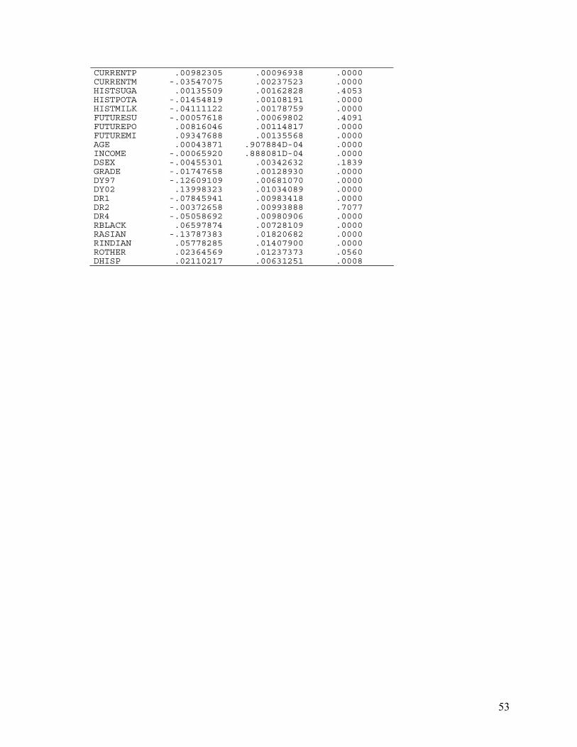
53
CURRENTP .00982305 .00096938 .0000 CURRENTM -.03547075 .00237523 .0000 HISTSUGA .00135509 .00162828 .4053 HISTPOTA -.01454819 .00108191 .0000 HISTMILK -.04111122 .00178759 .0000 FUTURESU -.00057618 .00069802 .4091 FUTUREPO .00816046 .00114817 .0000 FUTUREMI .09347688 .00135568 .0000 AGE .00043871 .907884D-04 .0000 INCOME -.00065920 .888081D-04 .0000 DSEX -.00455301 .00342632 .1839 GRADE -.01747658 .00128930 .0000 DY97 -.12609109 .00681070 .0000 DY02 .13998323 .01034089 .0000 DR1 -.07845941 .00983418 .0000 DR2 -.00372658 .00993888 .7077 DR4 -.05058692 .00980906 .0000 RBLACK .06597874 .00728109 .0000 RASIAN -.13787383 .01820682 .0000 RINDIAN .05778285 .01407900 .0000 ROTHER .02364569 .01237373 .0560 DHISP .02110217 .00631251 .0008