GEOL. CROAT. 49/2 289 - 293 3 Figs. ZAGREB 1996

RevielV paper

Economic Evaluation of Oil Exploration Projects

Arso PUTNIKOVIC and Hrvoje LIPOV AC

Key words: Economic evaluation, Reserve size, Monte-Carlo simulation.

Abstract This paper has a goa l 10 describe, in brief, the mathematical cal­

culations in economic evaluation of oi l exploration projects. Described arc calculation of geological risks, reserve size, develop­ment costs, production curves, production sharing and discoullting. Mathematical methods include cxpcc(Cd value theory, probability the­ory and Montc Carlo simulation . All is put toget her in Ihe fonn of a compllicr data input sheet, as a single procedure with Ihe purpose of giving the ,1Ilswcr is expected profit from a potential pro spec I big enough to justify the risk and money invested ill exploration.

I. INTRODUCTION

The economics of oil exp loration is the topic of many articlcs and academic discussions. Therc are many computer programs available on the markct, somc of which are very complex and can compute prof­itability in dctail. In exploration projects, which provc to be unprofitable to develop, the cause of failure is most frequcntly the incorrect evaluation of geological factors. However, it can be the ease that insuffie ienl and/or ovcrcomplex economic evaluation is the cause of such unproCitability, especially in marginal projects. Th e method described here is recommended for the eval uation of exploration projects because of its sim ­plicity and versatility of use in diferent fiscal-tax regimes.

2. DEFINITION OF PHASES

The procedure of economic evaluation of oil explo­ration projects can be divided into the following phases:

Phase 1. Geological estimates of the probability of suc­cess (factors for: the existence of a valid trap, reser­voir quality, seal, source rock, favourable migration -- coincidence of factors 10 produce a hydrocarbon accumulation);

INA -Naftaplin, Seklor za iSlrazivanjc i razvoj, Subiceva 29, I-IR-10000 Zagreb, Croatia.

PROCEEDINGS

Kljucnc rijcCi: ckonornska procjena, velicina rezervi, Monte-Carlo racunica.

Sazetak Rad ima za eilj opisali matemalicki postupak u ekonomskoj

ocjeni naftnih istrazllih projckala. Opisano jc racunanje s gcoloskim rizicima, racunanje kolicinc zaliha, razradnih lroskova, krivulja proi7.vodnje, raClll1anjc podjele proizvodnje i diskonliranjc. Ukljucene Sll postavke teorije ocek iv anc vrijednosti, teorijc vjcrojatnosti i Monle-Carlo sirnulacije. Svc jc objeclinjeno II jedinstveni poslupak, u obliku kompjulorskog programa, koji ima za cilj odgovoriti na pitanje jc Ii occkivana dobil projekt<l dovoljno velika cia opravda ulaganje kapilala II istra7.ivanja.

Phase 2. Eva luation of exploration costs (bonuses, seis­mic, drilling);

Phase 3. Evaluation of reserve parametcrs (acreage, bed thickness, accumulations);

Phase 4. Evaluation of field development parameters (price of oil, price of development well, required number of wells , cost of other dcvelopment, wcll li fc, perccntage of the oil sharing and the participation in the profit, taxes, choicc of the discount rate);

Phase 5. Compilation and intcgration calculation (probability theory, expected values and Monte Carlo multiplication's) and conclusion .

3. EXPLANATION OF THE CALCULATION PROCEDURE IN EACH PHASE

Disregarding the problcm of [he evaluation of a parameters' sizes, the calculation procedure for each phase is as follows.

PHASE I

The probable factors are:

• existence of a valid trap;

reservoir quality;

seal;

• source rock;

• favourable migration - co incidence or factor to pro­ducc a hydrocarbon accuillulation.

290

Geological estimates of probabilities arc expressed as a percentage and, assuming that the evaluated geo­logical probabilities arc independent, we can apply the multiplication theorem which will give the complex value - discovery probability.

Each probability factor can be subdivided into morc components but in such a case the overall probability of success (discovery probability) will be Jower.

As a rule each factor is expressed on a scale from 5-90%. 80-90% probability indicates a good factor (vcry low risk), 60-80% is probable (low risk), 40-60% is possible (medium risk), 20-40% is likely (high risk) and 5-20% represents the unlikely presence of a factor (very high risk).

The comparison of diHercnt exploration projects has sense only if probabilities are expressed using the same number of factors.

PHASE 2

The explorat ion costs arc evaluated from experience and current market prices. The sum of these also reprc­sent the risk that will have to be taken in case of failure as expressed financially. Many otherwise attractive pro­jects with a high expected value can be dropped because of this parameter alone, as the investor simply feels the amount or risk moncy is to high for him to take.

PHASE 3

Profit eva lu ation starts with thc evaluation of the sizc of the reserves. Here it is possible to:

a) eva luate the size or the reserves based on neigh­bouring fields so in this case no further compl icated calculations are necessary.

b) evaluate the parameters of reserve calculations, and by multiplication using the volumetric formula, reach the total size of the reserves.

Reserves (m)) = acreage x bed thickness x porosity x oil saturation x perccntagc of recoverab ility of total reserve x volumetric factor.

c) Many authors consider that the eva luation of paramcters such as a unique size does not represent the possible size of reserves, (as we can not be certain that the chosen size is realistic), but they recommend the parameters to be evaluated in the range from-to with or without stress on the most probable value, and that the usc or the special multipl ication procedure known as "Montc Carlo simu lation" lcads to the most probable reserves sIzes.

The Monte Carlo cal cui at ion procedure can be explained in the following way:

- imagine a graph with X and Y axes;

- the first parameter is put on X axis and its smallest and biggest value should be marked;

Y axis represents probability in the range from 0% to 100%;

Geologia Cronlica 49/2

100 % r----,."":-r--~~--------c_---___,

80%

.~ 60%

:g o o 0: 40%

20 %

2% O%'--"_L

~ 41 49 ~ U n ~ 87 M 102 Recoverable reserves (MM nil)

Fig. 1 Recoverable rese rves for Prospect "A", North Africa.

- the cumulative probabil ity is set for all the parameter

va lues on the X-axis slarting from the smallest one, by answering to the question "how sure are we lhat

the parameter value is at least that grea t". 'vVe should get a declining line with thc 100% valucs on thc Y­

axis up to 0% for the largest value;

- a random number in the rangc from 0 to 1 is chosen. II the chosen random number is i.e. 0.23, the value

23% on the Y axis must be found;

- from the drawn cumulative probability (declining lines) parameter values shou ld be read on the X-axis;

- the procedure is repeated for all the parameters;

- when the values are read off on the basis of the ran-

dom number for all the parameters enteri ng the for­mula, the value is calculated and the result is written

down. It is necessary to mention that it is not correct to multiply all the parameters with the same random

number. When the same random number is used all the time, then the small value of one parameter would be multiplied with a small value of other parameters, and the aim that we want to accompl ish is the result of testing with all the possible combi nations of the in­

coming parameters (the biggest x the biggest, the biggest x the smallest, the smallest x the smallest);

the procedure should be repeated until a satisfac tory number or written results is reached, usually 1000-1500 times;

- the written results are summed and the arithmetic

average is calculated through the probability distribu­tion in the following way:

- the groups are establ ished (classes) in which the sin­

gle results are sorted and this provides us the infonna­tion of how many single results each group contains. If the procedure is show n graphically throu gh the columns, the class with the highest column is so called modal class or the class where the most com ­

mon probability is found;

- the class is calculated as a percentage of the total number of cases and this number is multiplied with the middle number (lower class boundary + (upper -lower boundary) / 2) of each class;

PUlllikovic & LiPOV:1C: Economic EV:llu:lIion of Oil EXl>lor~lion Projecl.~ 291

"al;d "aD m;n max auaHIV ;1 90 120

I , ; I

" ;

I " 1.3 22 50

2:500 ~ 3ToD ~Bt9

; 'O~ ;

ooJ I ;

I.",

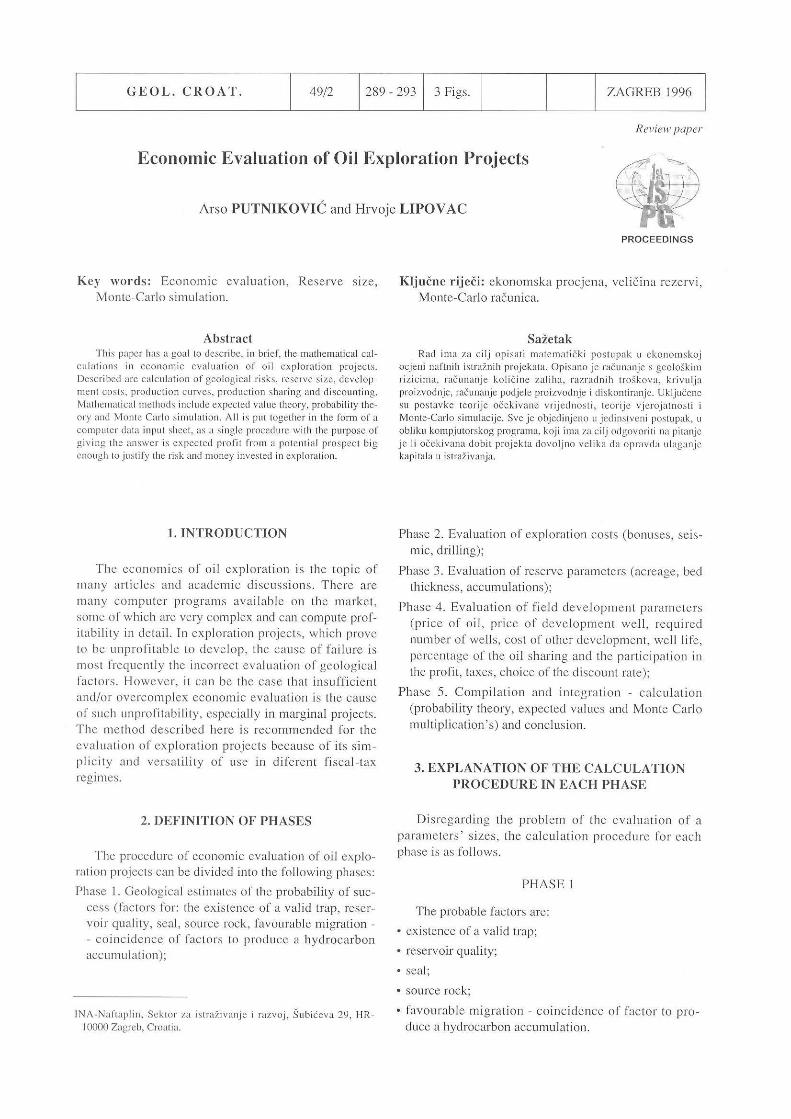
~ In" aav ; I ~ [(j]jQjjjjfI lO027' .006577 m;n moan max = -, 1 ",,"'., fMMm' l 1.B B.7 1B. ~ 3:5i< .. 6% numb" 01 w,II, 9 29 75

= ....... 70ii 75% om" fMM$1 -. 52 26' i% 9% ~ 19% f'iA[UE OF LOSS(MM$f 3

jQ 1.2. 1.3 , OF PROFIT IMM$1 9 ) VALUE OF 6

~ 1 vad,bla

r;;;;t;;;W =fm'/d,vl m. ..- --;;;:n max Prospect: Albania onshore

liS 120 i% 110 i% 95 i% 90

1i ii% Be • • , m"", i

I of 36 dg,API oil

Ig'~~:'~ feet*O.02832=Cubic metre metre*35.31 =Cubic Feet

I IU ~Eati I"

" roig.2 Economic cvaluat ion by Montc Carlo simu lati on; Prospect: A lbania onshore. IBTU ~ ;:~:; ;;;:;,:;;;'I;;';~':o~;~p:~,c;~ IKo"' ~, , i 0., c ..

- the sum o f the results gives the expected value or arithmetic average of a ll the results.

The advantage of the MonIC Carlo method versus the eval uation of reserve size based on the most proba­blc parameter va luc (dcscri bed in b) is tlwt it also takes into considcration all minimal and maximal parameter valucs. In thc dcsc ri bed cxample (rig. I) instead or a value of 5] x I 0" m ~ ror the most probable reserve size wc rcached the val ue of 64 x j ali m~ . Us ing the Montc­Ca rlo s imu lation we proved that a highe r val ue o f reserves was probable.

PI-lASE4

Th e required number of well s and th e ex pecled profit is calculated simultaneou sly to the quantification of expected reserves. The numbe r of well s is dete r­mined from the data o r initi a l and minimal da il y pro­duc tion or cach well (N EWENDORP, 1975) . Using " Darcy 's Law " a co rrelati on is made between the ex pected value or the bed thickness and the initial daily product ion. The rormula for the exponent ial production curve is being used and it is corrected for the number of ex pected negative well s (N EWEN DORP, 1975). The result of the poss ibl e well number can be checked on

ReMrv .. (NMm',

th e basis of data on the usual density of the develop­meIll well s grid applied to study area. Profit is calculat­ed on the basis o f the contractual terms deta iling the product ion percentages of profit share and is d iscounted at the chosen rate.

4. CONCLUSION (PHASE 5)

The ultimate aim is a comparison of expected ga in versus risk. In order to do thi s the expected va lue o f prorit (ar ithmetic average of profit multiplied by the probabil ity of di scovery) was compared with the excepted value of loss (m ultiplication of the exploration cost w ith the probabilit y of a ncgative we ll ) . .If the ex pected profitability valuc is higher than the ex pected loss va lue a decision can be undertaken as 10 either undertaki ng the ri sk or funile r evaluation.

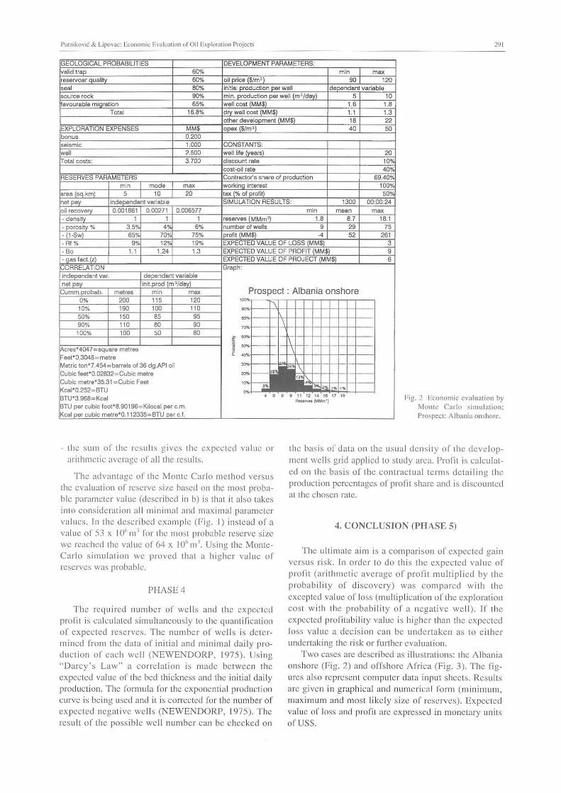
T wo cases are described as ill ust rations: the Albania onshore (Fig. 2) and o rrshore Arrica (Fi g . 3). The rig­ures al so represent computer data input sheets. Results arc gi ven in graphical and numcrical fo rm (minimum, maximum and most li kely size o f reserves). Expected val ue of loss and profi t are expressed in monetary unit s or uss.

292 Geologia Croatica 49/2

I I valid ,

I i i II sou,"a m,k ,

~ I , , II

~ ,oou,

well ~ Ii

olal '0""

mio ~

, area ('q.km) 3'

~ oel pay I oil ,.,ove>y 0.012802 0.02 - da",'ty 1 (ra,a>ve, (MMm') 29.4 69.5 110.3 - po>o,11y % lB.Oo/< 20% 22% loumbar otwall' 36 B2 287 - (I·Sw) 55% 60% 65% Ipro," (MM$) 529 1151 -Rt% 15% 20% 30% , VALUE OF LOSS (MMS) 9

- Bo .16 1.2 1.25 , VALUE OF PROFIT (MMS) 76 - 9a, ta,q,) , VALUE OF PROJEC (MM$) 67

I IGraph, , I var'able, ,I vor'able oel pay I'oil.prod, "/dey)

metre, m'n max Prospect: Africa offshore 0% 100 500 600 , 10% 95 450 490 50% BO 35 450 90% 65 200 300

60 100 150

'"~ ,melre,

Metr." 0'7., ,

Cub', , "'''. ",'n

BTU'; 'u . I

of 36 dg.API oil , mei re i Feet "Eilt OO,'~ ", fig. 3 Economic evaluation by

Montc Carlo simulation: BTU. per cu~!c foot ft 8.90196:=Kilocel per c.m. IK,al per cub', metre'O.I12335=BTU per of.

One inadequacy of the mcthod is that the political and financial risks are not being evaluated. Also only the expected value of a single prospect is considercd so it docs not includc the total geological potential of the area. This can be ovcrcomc by applying separate evalu­ations of political and financial risk (choosing an higher discount rate for example for those prospects which have such higher risks). For total evaluat ion of the geo­logical potential of the area a series of calcu lations as described herein have to be taken for each potential prospcct and, by summing the expected values, a mea­sure of the total geological potcntial of a certa in area can be achicvcd.

5, FORMULAS AND DEFINITIONS

I) Definition of probability:

P(D):= min

The probability of the event 0 is the ratio of all the favorable cases (m) to the number of all possible cas­es (n), where P = probability.

Prospect: Arrica orrshore.

2) Complex probability equals the probability product or each event

P(D I &D2& ... &Dn) = P(D I )xP(D2)x ... xP(DIl)

Pro bability "j~i", multiplication theorem. If the events D I, D2, ... Dn are independent, but they arc 110t mutually exclusive, in other words all of these or several of these, can appear sequentially, then this probability is called complex probability.

3) Formulas ror estab li shing the parameter values (NEWENDORP, 1975) based on the random nllmber (cf) if the known is: a) minimal and maximal value of parameter x:

x = xmin+cf*(xmax-xmin);

b) minimal, maximal andlhe most probable value of parameter x:

- for the x values s:; xmode

x=xm in+(xmaX-X111in)*sqrt(cf*(xlllodc-xrnin)/(xmax-xmin»

- for the x values :?: xmode

x=xmin+(xmax-xmin)*( I-sqrt« I-ct)*( 1-(xmodc-m in)1

(xmax -xmin»))

Putnikovic & LipoV;lC: Economic Evaluat ion or Oil Exploration Projects

considering that if c1' .:s; (xmode-xmi n)/(x max ­xmin) the first equat ion is used, a nd if e1' 2: (xmode-xmin)/(xmax -xmi n) the second one is app lied.

e) if the known cu mul ative parameter frequ e ncy is wri!len in the shape of: value of variable: 146 150 154 163 174

cUl1\u lative frequency : 0 0.4002 0.7959 0.9006 0.9674

the formula is:

x=x(n)+( cf-cf(n» *(x(n+ I )-x(n»/( ef(n+ I )-ef( n»

the calculation procedure is as fo llows:

the random number is chosen cf (from 0 to I)

the test is made if cf.:s; cf (2)

ifso than n:::ol and solve the equat ion for x if not question whether cr.s; cr (3)

if so than n:::o2 and solve the equation ror x if not question whether cr.s; c f (4)

if so than n:::o3 and solve the equation for x if not quest ion if of <; cf (5)

if so than n:::o4 and solve the equation for x if not than n:::o5 and solve the equation for x

lS I

4) Formula fo r the exponential declining production curve (used wh ile calculating the reserves per we ll ):

a= ln(q/q :,)/t

where a:::o dec linin g coeffi c ient; In :::0 natural loga ­rithm ; qt :::0 in it ial well production (tons/year) ; (h :::0

fina l wcl! production (tons/year); t :::o production time (year).

5) Rccovcrable reserves per well

dcln = ( l/a)*(ql -q2)

6) Number of wells per fie ld:

number of wells == total reserves / deln

7) Number of negative developmen t wells if the number of wells> 20

!leg = (2/15)*number of wells+ 3.33

if the number of wells .:s; 20

neg == (4/ 15)*nulllber of wells +0.67

(the numbers arc empirical)

293

8) time needed ro r the compl etion of the deve lopm ent wells

ti me = number of wel ls (posi ti ve and negative)/16

(time in years) assuming that 16 we ll s per year can be completed

9) d iscounted value of the development costs:

npvdeosl = development cost*e·O.I(,.,ime/2

10) discounted production value

income = reserves*priee (a/(a+.DV« l _e-t .("'j))!( I-c""')

a :::0 exponentia l c urve coeffi cien t; j :::0 discount rate; t :::0 time in years (field duration)

II ) discounted income

npvincome = ineome*e·O.]( .. ti m r/2

12) Defin it ion or the expected value 4) :

The expected value of some evcnt is the multiplica­tion or the events probability and the profit value of the same event.

e.g. emv = 20%*3 MM$ = 0.6 MM$

The expected value of the decision whether or not to accept the ri sk (expected value of a decis ion altcrna­tive) is the sum of the expected values o f all the pos­s ible events that are the subject of the decision.

e.g . SQOlo*$2MM = $1 MM Expected profit value

50%*-$1 MM = -$ O.SMM Expected value 01" loss

$1 MM~$O .5MM = $O.5MM

As the e xpected profit value is h ighcr than the

expected loss value the decision oj" accepting the risk should be made.

6. REFERENCE

NEWENDROP. P.D. (1975): D ecis ion analysis fo r pe tro leum exploration.- Penwell Boo ks, Tul sa, 5611'.

294 Geologia Croatiea 49(2