Embed Size (px)
Citation preview
This working paper has been developed within the Alcoa Advancing Sustainability Initiative to Research and Leverage
Actionable Solutions on Energy and Environmental Economics
WP FA15/2013
Economic Crisis and Elasticities of Car Fuels: Evidence for Spain
Mohcine Bakhat, José M. Labeaga Xavier Labandeira, Xiral López
2172 / 8437

1
Economic Crisis and Elasticities of Car Fuels: Evidence for Spain
Mohcine Bakhat a, José M. Labeaga a,b,*, Xavier Labandeira a,c, Xiral López a
a Economics for Energy. Doutor Cadaval 2, 3 E, 36202 Vigo, Spain b Departament of Economic Analysis II, UNED. Senda del Rey 11, 28040 Madrid, Spain c Rede and Departament of Applied Economics, Universidade de Vigo. Campus As Lagoas, 36310 Vigo, Spain
Abstract
This paper provides an updated calculation of the price and income responsiveness of Spanish consumers of car fuels, with an explicit exploration of the effects of the current economic crisis. We examine separate gasoline and diesel demand models using a set of estimators, including generalized method of moments and bias-corrected dynamic fixed-effect models, on a panel of 16 Spanish regions over the 1999-2011 period. The paper confirms the persistence of rather low own-price elasticities both for diesel and gasoline and both in short and long runs. It also shows that the crisis has slightly increased the price elasticity of demand, with a higher effect on gasoline than on diesel. On the contrary, the crisis has hardly affected the income elasticity of car-fuel demand. These updated results are obviously relevant for the current Spanish debate on the design and implementation of energy, environmental, fiscal and distributional policies. Moreover, given the duration and extent of the Spanish economic crisis, our conclusions may be also interesting and useful from an international perspective.
Keywords: diesel, gasoline, income, price, regions, panel data
JEL classification: C23, D12, Q41
* Corresponding author: [email protected] This paper could be carried out with the economic support of the Spanish Ministry of Economy and Competitiveness through its research project ECO2009-14586-C2-01 (Xavier Labandeira and Xiral López), Alcoa Foundation (Mohcine Bakhat and Xavier Labandeira). The usual disclaimer applies.

2
1. Introduction
From the mid 1990s and until the outbreak of the 2008 crisis, the demand of car fuels in Spain
saw an impressive and unprecedented evolution: from 1999 to 2007 gasoline and diesel
consumption grew at an average annual rate of respectively 5.1% and 6.5%, reflecting both the
strong growth of the Spanish economy and a limited responsiveness of demand to price changes
(which in this period respectively grew at annual average rates of 1.8% and 3.5%). Yet, three
years of deep crisis led to a completely different picture: between 2008 and 2011 gasoline and
diesel demand fell at an annual rate of respectively -2.4% and -1.8%, fuelled by strong increases
of prices (annual rates of 3.6% and 4.6%). It is clear that such a boom-and-bust evolution, as
depicted in Figure 1 later on, brings about remarkable environmental, economic or energy effects.
Given the huge changes seen in this market in the last few years, in this paper we are mainly
interested in providing an updated calculation of the price and income responsiveness of car fuel
demand in Spain. The availability of reliable demand elasticities is a necessary condition for a
proper economic evaluation of policies and strategies in this wide area. Given that Spain is
currently considering a wide reform of its tax system that may incorporate new and more intense
taxes on car fuels to reduce emissions and energy dependence, or due to the heated debate on
car-fuel pricing, the practical relevance of this piece research is clearly vindicated. Even outside
Spain, the results of this paper may be useful to anticipate the consequences of a pervasive and
long economic crisis on the demand of goods that are so relevant for welfare and economic
development.
Yet, there are also strong academic reasons for this paper. Although some authors have pointed
out that economic crises are likely to have effects on the price elasticities of goods, due for
instance to the larger incentives to react to prices that are associated to less availability of income
(Estelami et al., 2001), the academic evidence is so far quite limited. It is also true that the
literature generally considers that the price elasticity of demand is countercyclical, that is, sees
increases when the economy weakens (van Heerde et al., 2013). This seems to be especially the
case in products with a low-price elasticity, as energy goods, and in those that account for a big
share of total expenditure (Gordon et al., 2013). However, the actual empirical evidence on the
variation of demand elasticities at times of economic crisis is very limited, if it exists at all.

3
It is well known that the Spanish economy has been much shaken by the global financial crisis
and its aftermath, being one of the developed countries that suffered the sharpest falls in growth
and unemployment after 2008. As a result, the crisis saw Spanish energy consumption
plummeting as households cut consumption spending and Spanish producers scaled down their
purchases of energy input. Understanding the effects of the crisis on Spanish energy demand,
but particularly on car-fuel demand, is especially important at least for two reasons. First, fuel
consumption is an important source of public revenues and thus a likely source of disruptive
effects on government budgets. Second, price and income elasticities of demand are important
for the choice of domestic energy policies and thus have important implications for energy and
environmental policies. Therefore, omitting structural changes in consumer responsiveness to
price and income may result in misleading analysis, advice and policies (Hughes et al., 2008).
This paper provides an updated calculation of the price and income responsiveness of Spanish
consumers of car fuels, with one of the first explorations of the effects of the current economic
crisis. We examine separate gasoline and diesel demand models using a set of estimators,
including generalized method of moments and bias-corrected dynamic fixed-effect models, on a
panel of Spanish regions covering the 1999-2011 period. We try to reconcile some apparently
contradictory evidence available for Spain, dealing carefully with the main econometric problems
found for the estimation of this kind of demand models.
The reminder of this paper is structured as follows. Section 2 reviews the related literature.
Section 3 describes the methodology used in this analysis. Section 4 presents the empirical
analysis discussing the data used and reporting the core results of various estimation techniques.
The last section concludes.
2. Literature review
Reduced-form demand models have been extensively used in the specification of automobile fuel
demand. Using either static or dynamic forms, in this approach model estimation can have
different forms depending on the type of data available, which can be purely time-series data,
cross-section data or panel data. In the first category, when data are purely temporal, the partial
adjusted model (PAM) stands as one of the preferred alternatives to analyze fuel demand and
estimate different elasticities. In contrast to static models that provide average elasticities, the

4
PAM is a dynamic model that yields short and long run elasticities (Hothakker et al., 1974). The
rationale behind this model is that markets are not perfect and some frictions, such as consumer
habits, preclude reaching the proper equilibrium. Thus, a model of this type can be defined to
capture the limited capability of consumers to adjust immediately to the long-run equilibrium of
consumption in response to change in price, income, population and other factors (Li et al.,2010;
Banaszak et al.1999; Al-faris, 1997; Sterner and Dahl, 1992). Yet other approaches, e.g. using
co-integration techniques, have stressed the need to account for the possible non-stationary
nature of the time series. Some initial evidence points into the direction that failure to reach
stationarity may lead to overestimation of long-run price elasticities (Eltony and Al-Mutairi, 1995;
Samimi, 1995; Ramanathan; 1999; Dahl and Kurtubi, 2001). In line with the cointegration
technique, the autoregressive distributed lag (ARDL) bounds-testing approach developed by
Pesaran et al. (2001) has been used in various empirical studies to determine long-run elasticities
(Boshoff, 2012; Akinboade et al., 2008; De Vita et al., 2006).
During the last decade, developments of panel-data econometric methods allowed for the
estimation of energy demand models by combining time-series and cross-section data. The
increasing interest in the use of panel-data modeling is largely due to the ability of this technique
to sort several econometric problems. For instance, panel data models have offered a solution to
the problem of bias caused by unobserved heterogeneity, a common issue in fitting the models
with cross sectional data sets. Moreover, panel-data models can account for dynamics that are
difficult to detect with cross-sectional data (Hsiao, 2003; Baltagi, 2001; Wooldridge, 2002).
In this context, the fact that fuel consumption decision is made at the household level means that
demographic profiles of households play a major role in automobile fuel consumption
(Schmalensee and Stoker, 1999; Yatchew and No, 2001; Kayser, 2000). There are also several
applications that used aggregate data to implement estimations at local or regional levels. Baltagi
et al. (2003) employed a panel dataset from 21 French regions and compared the performance of
different sets of homogenous and heterogenous estimators in the calculation of gasoline price
and income elasticities. They found that standard homogenous estimators perform better than
their counterparts, obtaining short-run price and income elasticities for gasoline of respectively
-0.093 and 0.2. Other European studies at a regional level confirmed the prevalence of very small
gasoline short-run elasticities: Baltagi and Griffin (1997) found short-run price and income

5
elasticities for gasoline to be -0.09 and 0.5, with a larger long-run price elasticity of -1.391. Liu
(2004), who considered a set of different energy types and differentiates residential and industrial
sectors, used the one-step GMM estimator to a PAM (Arellano and Bond, 1987), reporting a
larger value (in absolute terms) of the short-run gasoline price elasticity and a comparatively
lower income elasticities in the residential sector. More recently, Pock (2010) reported very small
short-run effects of price and income changes in gasoline consumption (respectively -0.09 and
0.065), which would be probably due to the gradual and generalized switch to diesel cars.
Although studies on the demand for fuels in advanced countries are rather abundant in the
economic literature2, there is a limited number of papers for the Spanish case. Some authors
have estimated the price and income elasticities at the household level based on complete
demand models: Labeaga and López-Nicolás (1997) used a flexible Almost Ideal Demand
System (AIDS), with a special treatment to the problems of zero expenditure and unobserved
heterogeneity, and reported price and income elasticities for gasoline of respectively -0.536 and
0.429. Labandeira and López-Nicolás (2002) followed the same methodology for a different time
spam and yielded -0.08 and 0.99 for respectively price and income elasticities of car-fuel
demand. A study of Labandeira et al. (2006), based on a modified form of the AIDS model
(Quadratic-AIDS), estimated price and income elasticities of household energy goods and found
that the price elasticity of car fuels ranged between -0.11 and -0.058, while income elasticity was
between 1.36 and 1.79. This contrasted with Romero-Jordan et al. (2010), who found larger car-
fuel price elasticities, ranging between -0.64 and -0.32, and income elasticities (between 0.92 and
1.45). Such observed differences may be due to the varying time frames and to the different
methodological approaches.
Other authors followed a different approach by using aggregate data of peninsular Spanish
regions. Danesin and Linares (2013) estimated the aggregate price and income elasticities for
both gasoline and diesel. Using a panel data model based on a set of homogeneous estimators,
they reported a short-run gasoline price elasticity in the (-0.93, -0.29) interval, and a long-run
price elasticity of -0.69, with gasoline income elasticities found to be non-significant. For diesel,
short-run price elasticity estimates ranged between -0.22 and -0.21, while short-run income
1 These values correspond to the GLS-AR(1), which shows the best performance. 2 Dahl and Sterner (1991), Sterner and Dahl (1992), Dahl (1995), Goodwin et al. (2004), de Jong and Gunn (2001), Graham and Glaister (2002,2004) and Basso and Oum (2007) have provided surveys of the existing literature on fuel demand elasticities.

6
elasticity were found to be between 0.35 and 0.46. González-Marrero et al. (2012) used the one-
step system GMM along with other standard estimators to compute price and income elasticities.
They found that one-step system GMM estimator performs better than its counterparts, yielding
short and long run gasoline price elasticities of respectively -0.292 and -0.69, with non-significant
estimates for diesel and income elasticities.
3. Methodology
3.1. Econometric model
In this paper we employ a PAM with a static representation of a long-run demand function in
which (GAS/CAR)* is the desired fuel (gasoline or diesel) consumption per vehicle, as in Baltagi
and Griffin (1983; 1997). Assuming a Cobb Douglas relationship between desired demand and its
drivers, Equation (1) defines the long-run demand curve as a function of the real price of the car
fuel, , and a set of covariates, real income per capita and cars per capita .
To reduce the information bias, total drivers are used instead of total population. The long-run
price elasticity of demand is denoted as β, with and as vectors of coefficients that describe
the responsiveness of the long-run level of demand to the non-price covariates, and α as a
constant.
(1)
Following Houthakker et al. (1974), a function is introduced to capture the limited capability of
consumers to adjust immediately to the long-run equilibrium level of consumption in response to a
change in price, income and other variables. Equation (2) indicates this limited capability in the
form of a partial-adjustments constraint, designated by a parameter that captures the year-to-
year inertia of habit persistence of fuel consumers, taking values between zero and one.
⎟⎠⎞⎜
⎝⎛
PP
CPIMG ⎟
⎠
⎞⎜⎝
⎛NY
⎟⎠
⎞⎜⎝
⎛NCAR
γ δ
δγβ
α ⎟⎠
⎞⎜⎝
⎛⎟⎠
⎞⎜⎝
⎛⎟⎟⎠
⎞⎜⎜⎝
⎛=⎟
⎠
⎞⎜⎝
⎛NCAR
NY
PP
CARGAS
GDP
MG*
θ
7
(2)
Adding region and time subscripts, and the total fleet per km of roads to control for the saturation
level of the road network, the classical dynamic demand equation for fuel per vehicle is
expressed as
(
(3)
with , , where denotes a region–specific effect and is
white noise. A trend is included in the specification so that technical progress can differently affect
demand for fuel through time. Under formulation (3), the short-run elasticities of car-fuel demand
per car with respect to per capita income, real price, total cars per driver and level of saturation
are respectively and . The corresponding long-run responses are given by
and , with (1−θ) as the speed of adjustment to the long-run equilibrium. Note that the
stock of cars thus enters both as dependent and independent variable. Therefore, the short and
long run responses of car-fuel demand, relative to changes in the saturation level, are
respectively (1+θδ) and (1+ δ).
Given that an important goal of this paper is to analyze consumer responses to price changes
during the time span 1999-2011, which includes the crisis period, the following empirical model is
tested3
( ) titi
tiCPI
MGcrisis
tititi
uTrendSATtiN
CAR
PPDN
YCARGAS
CARGAS
,,
,,1,,
,lnln
ln)(lnln)1(lnln
+++⎟⎠
⎞⎜⎝
⎛+
⎟⎟⎠
⎞⎜⎜⎝
⎛++⎟
⎠
⎞⎜⎝
⎛+⎟⎠
⎞⎜⎝
⎛−+=⎟⎠
⎞⎜⎝
⎛
−
θµθϕθδ
λθγθβθαθ
(
(4)
3 In the empirical application we also allow for different income effects due to the crisis.
θ
⎟⎟⎟⎟⎟
⎠
⎞
⎜⎜⎜⎜⎜
⎝
⎛
⎟⎠
⎞⎜⎝
⎛
⎟⎠
⎞⎜⎝
⎛
=
⎟⎟⎟⎟⎟
⎠
⎞
⎜⎜⎜⎜⎜
⎝
⎛
⎟⎠
⎞⎜⎝
⎛
⎟⎠
⎞⎜⎝
⎛
−− 1
*
1 t
t
t
t
CARGASCARGAS
CARGASCARGAS
( ) ti
titiCPI
MG
tititi
uSAT ti
NCAR
PP
NY
CARGAS
CARGAS
,
,,,1,,
,ln
lnlnlnln)1(lnln
++
⎟⎠
⎞⎜⎝
⎛+⎟⎟⎠
⎞⎜⎜⎝
⎛+⎟
⎠
⎞⎜⎝
⎛+⎟⎠
⎞⎜⎝
⎛−+=⎟⎠
⎞⎜⎝
⎛
−
θϕ
θδθγθβθαθ
ititiu εµ +=, TtNi ,..,1,,...,1 == iµ itε
θδθγθβ ,, θϕ
δγβ ,, ϕ
8
where a dummy variable equal to 1 between 2008 and 2011 and zero otherwise. Thus,
the short-run price elasticity in the crisis period will be , where captures the effects of
the crisis period and is expected to be negative. In addition, we included a trend that proxies the
technological evolution for gasoline and diesel vehicles.
3.2. Model estimation
To calculate the different elasticities of fuel demand we need to estimate Equations (3) or (4),
which is subject to two main methodological challenges: unobserved heterogeneity as a source of
effects on the explanatory variables, and the presence of a lagged dependent variable in a panel-
data context. Regarding the former, simply regressing fuel consumption on a set of regional
explanatory variables may lead to biased estimates unless all relevant variables can be observed.
While some of these control variables are periodically published by public entities or statistical
agencies, other variables are unlikely to be easily accessed or recorded and thus researchers
relying solely on observable variables make the assumption of “unconfoundness” (Imbens and
Woodridge, 2009). In doing so, they actually produce incorrect measures of demand
responsiveness of consumers and infer spurious policy effects. Nevertheless, under the
assumption that the effects of time-invariant factors can be linearly separated, the regional fixed-
effects will remove the bias induced by observed and unobserved heterogeneity.
A fixed-effect transformation such as time-demeaning all the variables in Equation (4) has the
form , where and , with as the vector of
the time-varying right-hand variables. The estimator from this regression would be consistent only
if the current values of explanatory variables (real price, real income, fleet per capita, and roads
saturation) are completely independent of past realizations of the dependent variable (fuel
consumption), i.e., if . Obviously, the inclusion of lagged-dependent variables
violates the strict exogeneity in this equation. Therefore, the fixed-effects estimator is inconsistent
and biased in dynamic models. The least squares dummy variables (LSDV) or within-groups
estimate is downward biased when considering model (4), and this bias would be especially
severe when the autoregressive coefficient is high or the number of time periods, T, is
small (Nickell, 1981; Roodman 2006).
Dcrisis
λθγ + λ
( ) εβθ ++−= − xyyt tt t~~1~ *
1 yyy it it −=~ xxx it it −=~ xit
tsxE itis ,,0)( ∀=ε
( )θ−1

9
To obtain consistent estimates, under the assumption that unobserved heterogeneity exists but it
is time-invariant, Equation (4) is estimated using a dynamic generalized method of moments
(GMM) estimator4. The basic estimation procedure consists of two essential steps: first, the
dynamic model in Equation (4) is transformed5 to eliminate the unobserved effects and
subsequently the model is estimated using GMM, including lagged values of explanatory
variables as instruments for the current explanatory variables. For these instruments to be valid,
they must fulfill two conditions: to provide a source of variation of current explanatory variables,
and lagged values have to yield an exogenous source of variation for current fuel consumption. In
our empirical analysis we further examine the validity of the exogeneity assumptions using a
battery of tests. Under the assumption of exogeneity, the orthogonality conditions satisfy
. However the procedure still has several shortcomings:
first, differencing the equations in levels may reduce the power of the tests by reducing the
variations in the explanatory variables; second, it has been argued that variables in levels may be
weak instruments for first differencing equations (Arellano and Bover, 1995); and, finally, first-
differencing may aggravate the effects of measurement errors on the dependent variable
(Griliches and Hausman, 1986).
Arellano and Bover (1995) and Blundell and Bond (1998) suggested an improved version of the
GMM estimator by also including the equations in levels in the estimation procedure. The
approach is based on a system of equations that includes equations in both levels and
differences, and where the first-differenced variables are used as instruments for the equations in
levels. This gives rise to a “system” GMM estimator that hinges on estimating the following
system,
(5)
Unfortunately, equations in levels in this system still contain unobserved heterogeneity. To deal
with this issue we assume that any correlation between explanatory variables and unobserved
4 This approach was introduced by Holtz-Eakin, Newey and Rosen (1988) and Arellano and Bond (1991), and further developed in a series of papers including Arellano and Bover (1995) and Blundell and Bond (1998). 5 That is, any transformation that permits to rule out the unobserved component. Although we will later refer to first differences, there are other alternatives such as orthogonal deviations (see Arellano and Bover, 1995).
( ) ( ) 10 syExE itsititsit ∀== −− εε
εβλα itit
it
it
it
it
it
xx
yy
yy
+⎥⎦
⎤⎢⎣
⎡
Δ+⎥⎦
⎤⎢⎣
⎡
Δ+=⎥
⎦
⎤⎢⎣
⎡
Δ −
− ***
1
1
10
heterogeneity is constant over time (one would suspect that variables such as real income, fleet,
and saturation are correlated with unobserved effects that characterize each region). In this
setting, the system GMM estimator under the extra set of orthogonality conditions6 yields efficient
estimates while controlling for time-invariant unobserved heterogeneity and the dynamic
relationship between current values of the explanatory variables and past values of the
dependent variable.
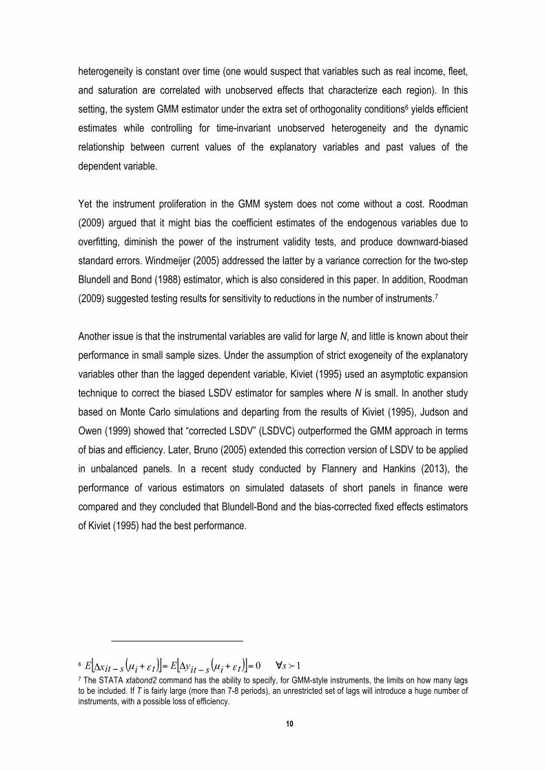
Yet the instrument proliferation in the GMM system does not come without a cost. Roodman
(2009) argued that it might bias the coefficient estimates of the endogenous variables due to
overfitting, diminish the power of the instrument validity tests, and produce downward-biased
standard errors. Windmeijer (2005) addressed the latter by a variance correction for the two-step
Blundell and Bond (1988) estimator, which is also considered in this paper. In addition, Roodman
(2009) suggested testing results for sensitivity to reductions in the number of instruments.7
Another issue is that the instrumental variables are valid for large N, and little is known about their
performance in small sample sizes. Under the assumption of strict exogeneity of the explanatory
variables other than the lagged dependent variable, Kiviet (1995) used an asymptotic expansion
technique to correct the biased LSDV estimator for samples where N is small. In another study
based on Monte Carlo simulations and departing from the results of Kiviet (1995), Judson and
Owen (1999) showed that “corrected LSDV” (LSDVC) outperformed the GMM approach in terms
of bias and efficiency. Later, Bruno (2005) extended this correction version of LSDV to be applied
in unbalanced panels. In a recent study conducted by Flannery and Hankins (2013), the
performance of various estimators on simulated datasets of short panels in finance were
compared and they concluded that Blundell-Bond and the bias-corrected fixed effects estimators
of Kiviet (1995) had the best performance.
6 7 The STATA xtabond2 command has the ability to specify, for GMM-style instruments, the limits on how many lags to be included. If T is fairly large (more than 7-8 periods), an unrestricted set of lags will introduce a huge number of instruments, with a possible loss of efficiency.
( )[ ] ( )[ ] 10 stiy sitEtix sitE ∀=+Δ −=+Δ − εµεµ

11
4. Empirical application
4.1. Data
Our dataset consists of a panel of 16 Spanish administrative regions and covers the 1999-2011
period (annual data)8. Variables include fuel consumption, disaggregated in regional gasoline and
diesel consumption and obtained from the annual reports of National Commission of Energy
(CNE its acronym in Spanish); real gasoline and diesel prices, obtained from the Spanish Ministry
of Industry; regional Spanish population, from the National Institute for Statistics (INE its acronym
in Spanish); number of gasoline and diesel cars (an important determinant of the long-run
evolution of car traffic), sourced from the General Direction of Traffic (DGT its acronym in
Spanish); total kilometers of regional roads, obtained from the Ministry of Infrastructures
(Fomento in Spanish); and household disposable income and price index, both obtained from the
INE. As already mentioned, the effect of technical progress on car-fuel consumption is taken into
account by including a trend.9
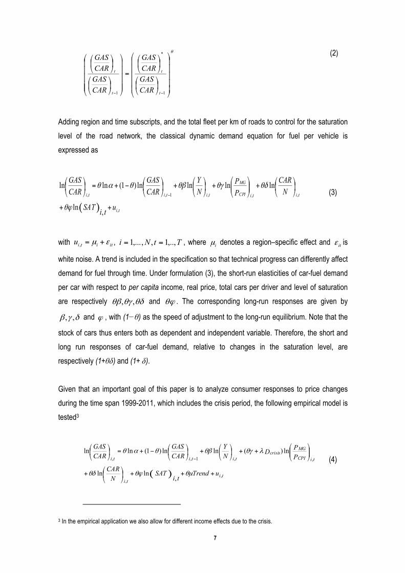
Figure 1 depicts the evolution of consumption and real prices of both gasoline and diesel between
1999 and 2011. Since 1999 diesel demand has been steadily increasing, while demand for
gasoline has decelerated its growth since 2001. Indeed, due to a favorable tax regime, diesel now
makes more than 80% of Spanish demand of car fuels and thus is in a near-saturation stage.
However, this growth has been stopped by the recent economic crisis, which strongly affected
both gasoline and diesel demand. Spain annual diesel consumption in 2011 was around 31
million litres, or 30% lower than it would have been if the pre-2007 trend in diesel consumption
annual growth of 5.6% had continued. Similarly, Gasoline consumption in 2011 was about 6
million litres, or 26% lower than it would have been if the 2004-2006 annual growth of 1.2% had
been maintained. In addition, high unemployment during the recent economic contraction has
reduced disposable income and has strongly affected car sales and thus the quality of the fleet.
For instance, the growth rate of diesel fleet dropped from 10% between 2004 and 2006 to 1.2% in
2011.
8 Ceuta, Melilla and Canary Islands were excluded from this analysis as they have a special tax regime that may distort the results. 9 We are aware that in a model estimated in first differences the first difference of a trend is just a constant.

12
Figure 1 shows that gasoline and diesel price trends were broadly similar over the period 1999-
2011. Real prices increased at a faster rate between 1999 and 2000, bringing about concern and
demonstrations across Spain and Europe. After a price-decreasing interval between 2001 and
2003, prices went up again with sharp spikes brought about by the outbreak of the crisis and a
strong rebound at the end of the analyzed period.
Figure 1. Gasoline and diesel real prices (Euros/litres) and annual consumption (Million litres) in Spain (1999-2011)
Source: The authors with data from Ministry of Industry and CNE.
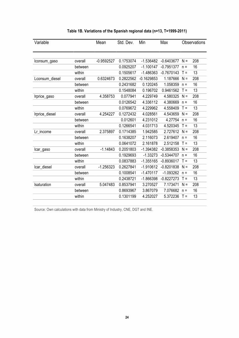
As this study is based on panel data analysis, it is important to assess the variations of the
variables over time and across regions. Table 1A in the Appendix summarizes the extent of data
variation, both inter and intra regionally for the key variables: gasoline and diesel consumption
per car, gasoline and diesel prices per capita, income, cars per capita and road saturation. For
diesel, price and number of cars per capita, variations were more pronounced within the same
region across the years than between regions, whereas the variation of consumption per car was
more remarkable between regions than within the same region. For gasoline, price and
consumption variations were more intense within each region than between regions, while the
variation of gasoline vehicles was more remarkable in per capita terms than within regions.
0
5
10
15
20
25
30
50
60
70
80
90
100
99 00 01 02 03 04 05 06 07 08 09 10 11
RP_DIESEL RP_GASOGASO DIESEL

13
Finally, road saturation variation was predominantly between regions, whist the variation of real
income was less pronounced within the region than between regions.
4.2. Results
Tables 1 and 2 report the main results. We estimate the first-order autoregressive model by OLS
and LSDV as reference specifications. The coefficients of the lagged-dependent variable
obtained from these two estimators provide the bound limits that are a useful check on the results
from a theoretically superior estimator (Bond, 2002). In particular, while the naïve OLS estimator
overestimates the coefficient of the lagged dependent variable because regional fixed effects are
not accounted for10, the LSDV estimator produces a downward bias. The preceding tables only
report three alternatives to the reference specifications: the Anderson-Hsiao (HS), Arellano-Bond
(AB) and Blundell-Bond (BB Full) estimators. The BB Full version involves the use of the full
instrument set available in the data11 and, as explained earlier, the model contains a lag of the
endogenous variable and several exogenous explanatory variables. We use as instruments the
dependent variable with a lag of two or more periods, also considering the results for a corrected
LSDV estimator (Kiviet, 1995; Bruno, 2005).
Tables 1 and 2 also supply the heterosckedasticity-consistent asymptotic standard errors in
parenthesis, the t-statistic for the linear restriction test under the null hypothesis of non-
significance, and the Hansen test of the overidentifying restrictions. This test is asymptotically
distributed as χ 2 under the null of no correlation between the instruments and the error term.
Besides, the previous tables report mi , which is a serial correlation test of order i (i = 1, 2) using
the residuals in first differences, asymptotically distributed as N(0, 1) under the null of no serial
correlation (see for details Arellano and Bond, 1991). The tests present no evidence of second-
order autocorrelation at 5% significance level in the case of gasoline, although this is rejected in
the case of diesel12. Based on the robust Hansen test, the overidentification restrictions are valid
10 The Hausman test rejects the null and concludes that random effects are not appropriate. 11 We have estimated several alternatives of the BB model in which we restrict the number of instruments following the procedure outlined in Roodman (2009). They produce pretty similar short and long run elasticities to the ones presented and discussed later on. We have also estimated the model using the LSDV estimator proposed by Kiviet (1995) and Bruno (2005). Although we do not present these results in the paper, they are available upon request. 12 We have tried with instruments with lags of three or more periods, allowing for the presence of measurement error in the consumption of diesel, although the value of the test for second-order autoregressive residuals fails.

14
at 5% significance level for both diesel and gasoline13. The F- and χ 2 - statistics reject the null
hypothesis that estimated parameters are jointly equal to zero in the proposed estimators for
diesel and gasoline.
Table 1. Estimates of the diesel dynamic demand model
VARIABLES OLS LSDV AH AB BB_Full Lag of diesel consumption/car
0.981*** 0.738*** 0.733*** 0.581*** 0.657***
(0.0146) (0.0744) (0.0753) (0.0801) (0.100)
Trend -0.000597 -0.00910** -0.00879** -0.0159*** -0.0158***
(0.00158) (0.00423) (0.00379) (0.0049) (0.00333)
Diesel real price -0.106*** -0.0839** -0.0645** -0.0601** -0.0913***
(0.0308) (0.0299) (0.0322) (0.0303) (0.0292)
CrisisXprice -0.00496*** -0.00517*** -0.00483*** -0.00488*** -0.00595***
(0.000845) (0.000959) (0.000852) -0.000983 (0.00105)
Real Income 0.0489*** 0.298** 0.283*** 0.389*** 0.325**
(0.0178) (0.114) (0.0891) (0.141) (0.150)
Cars per driver 0.0141 0.0198 -0.00471 0.0939 0.0679
(0.0198) (0.0649) (0.0563) (0.0868) (0.0742)
Road saturation -0.00609 -0.144 -0.153* -0.298*** -0.111**
(0.00429) (0.103) (0.0885) (0.0968) (0.0385)
Constant 0.359*** 0.599 0.583 1.261** 0.532*
(0.133) (0.524) (0.454) (0.521) (0.259)
T 12.73*** 8.75*** 4.58** 4.47** 10.91***
m1 -3.107*** -2.93
m2 -1.968** -1.74*
Jointly zero coefficients 2116*** 862*** 85054*** 3378*** 442***
Hansen 13.57ª 14.66
Observations 192 192 176 176 192
R-squared 0.988 0.965
Number of ccaa 16 16 16 16 16
Number of instruments 70 81 ª Hansen test is not computable here, so we report Sargan test instead.
Notes: Standard errors in parentheses; *** p<0.01, ** p<0.05, * p<0.1; BB_Full is Blundell and Bond estimator considering all the instruments; Hausman test is 17.98, so the random effects hypothesis is rejected at a 1% level of significance.
Source: the authors.
13 Since the tests for the validity of the instruments do not reject the null there might be a misspecification problem, even though we expect that it does not affect the elasticity figures.
15
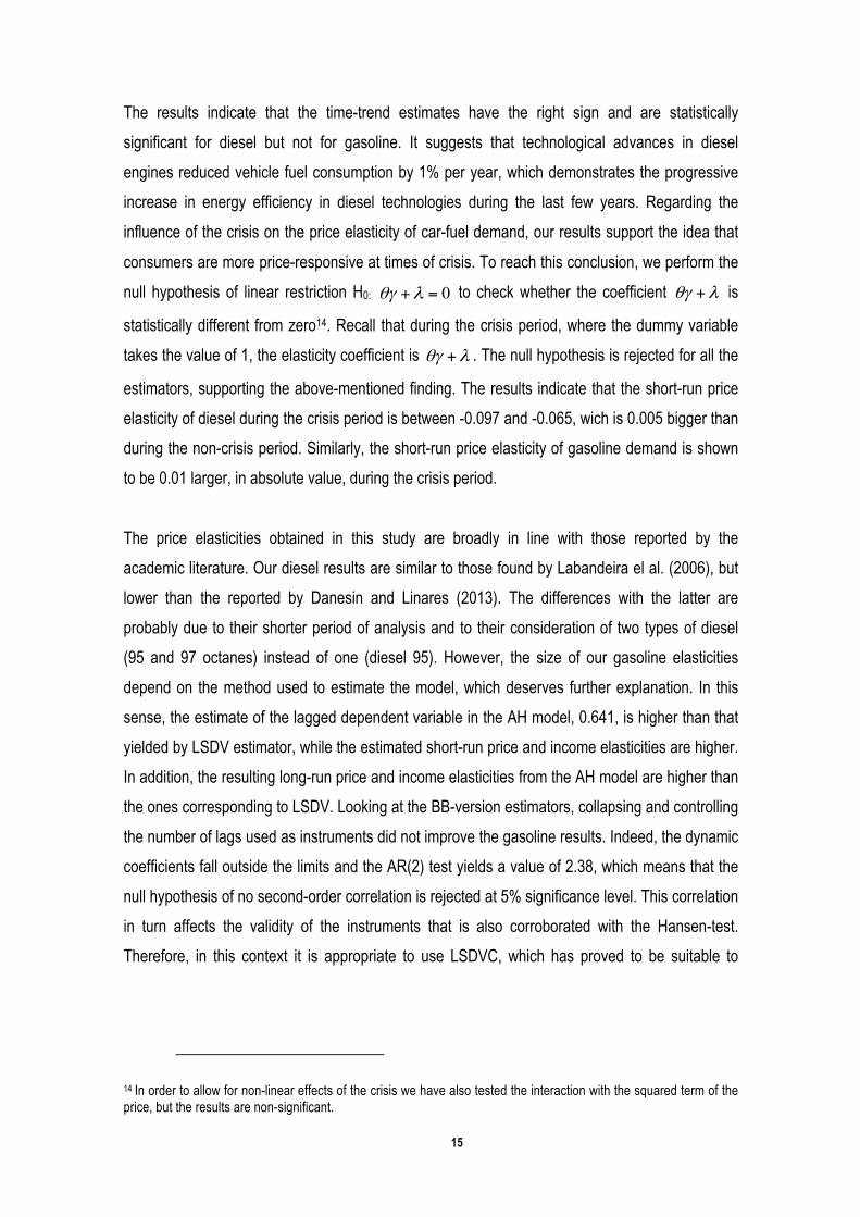
The results indicate that the time-trend estimates have the right sign and are statistically
significant for diesel but not for gasoline. It suggests that technological advances in diesel
engines reduced vehicle fuel consumption by 1% per year, which demonstrates the progressive
increase in energy efficiency in diesel technologies during the last few years. Regarding the
influence of the crisis on the price elasticity of car-fuel demand, our results support the idea that
consumers are more price-responsive at times of crisis. To reach this conclusion, we perform the
null hypothesis of linear restriction H0: 0=+λθγ to check whether the coefficient is
statistically different from zero14. Recall that during the crisis period, where the dummy variable
takes the value of 1, the elasticity coefficient is . The null hypothesis is rejected for all the
estimators, supporting the above-mentioned finding. The results indicate that the short-run price
elasticity of diesel during the crisis period is between -0.097 and -0.065, wich is 0.005 bigger than
during the non-crisis period. Similarly, the short-run price elasticity of gasoline demand is shown
to be 0.01 larger, in absolute value, during the crisis period.
The price elasticities obtained in this study are broadly in line with those reported by the
academic literature. Our diesel results are similar to those found by Labandeira el al. (2006), but
lower than the reported by Danesin and Linares (2013). The differences with the latter are
probably due to their shorter period of analysis and to their consideration of two types of diesel
(95 and 97 octanes) instead of one (diesel 95). However, the size of our gasoline elasticities
depend on the method used to estimate the model, which deserves further explanation. In this
sense, the estimate of the lagged dependent variable in the AH model, 0.641, is higher than that
yielded by LSDV estimator, while the estimated short-run price and income elasticities are higher.
In addition, the resulting long-run price and income elasticities from the AH model are higher than
the ones corresponding to LSDV. Looking at the BB-version estimators, collapsing and controlling
the number of lags used as instruments did not improve the gasoline results. Indeed, the dynamic
coefficients fall outside the limits and the AR(2) test yields a value of 2.38, which means that the
null hypothesis of no second-order correlation is rejected at 5% significance level. This correlation
in turn affects the validity of the instruments that is also corroborated with the Hansen-test.
Therefore, in this context it is appropriate to use LSDVC, which has proved to be suitable to
14 In order to allow for non-linear effects of the crisis we have also tested the interaction with the squared term of the price, but the results are non-significant.
λθγ +
λθγ +
16
correct the bias in the LSDV estimator and in the case of small samples where the GMM
estimator lacks efficiency15.
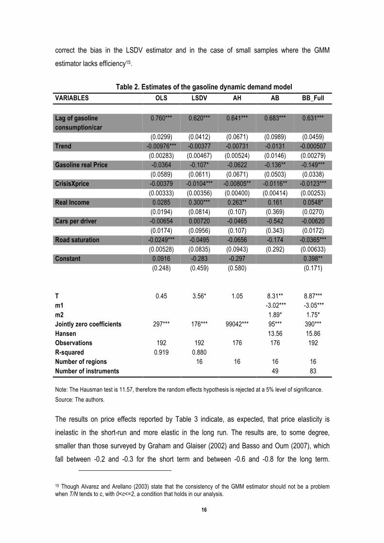
Table 2. Estimates of the gasoline dynamic demand model
VARIABLES OLS LSDV AH AB BB_Full Lag of gasoline consumption/car
0.760*** 0.620*** 0.641*** 0.683*** 0.631***
(0.0299) (0.0412) (0.0671) (0.0989) (0.0459) Trend -0.00976*** -0.00377 -0.00731 -0.0131 -0.000507 (0.00283) (0.00467) (0.00524) (0.0146) (0.00279) Gasoline real Price -0.0364 -0.107* -0.0622 -0.136** -0.149***
(0.0589) (0.0611) (0.0671) (0.0503) (0.0338) CrisisXprice -0.00379 -0.0104*** -0.00805** -0.0116** -0.0123***
(0.00333) (0.00356) (0.00400) (0.00414) (0.00253) Real Income 0.0285 0.300*** 0.263** 0.161 0.0548*
(0.0194) (0.0814) (0.107) (0.369) (0.0270) Cars per driver -0.00654 0.00720 -0.0465 -0.542 -0.00620
(0.0174) (0.0956) (0.107) (0.343) (0.0172) Road saturation -0.0249*** -0.0495 -0.0656 -0.174 -0.0365***
(0.00528) (0.0835) (0.0943) (0.292) (0.00633) Constant 0.0916 -0.283 -0.297 0.398** (0.248) (0.459) (0.580) (0.171)
T 0.45 3.56* 1.05 8.31** 8.87*** m1 -3.02*** -3.05*** m2 1.89* 1.75* Jointly zero coefficients 297*** 176*** 99042*** 95*** 390*** Hansen 13.56 15.86 Observations 192 192 176 176 192 R-squared 0.919 0.880 Number of regions 16 16 16 16 Number of instruments 49 83
Note: The Hausman test is 11.57, therefore the random effects hypothesis is rejected at a 5% level of significance.
Source: The authors.
The results on price effects reported by Table 3 indicate, as expected, that price elasticity is
inelastic in the short-run and more elastic in the long run. The results are, to some degree,
smaller than those surveyed by Graham and Glaiser (2002) and Basso and Oum (2007), which
fall between -0.2 and -0.3 for the short term and between -0.6 and -0.8 for the long term.
15 Though Alvarez and Arellano (2003) state that the consistency of the GMM estimator should not be a problem when T/N tends to c, with 0<c<=2, a condition that holds in our analysis.

17
However, they are in line with those reported by Pock (2010) for the EU contries (short-run:
-0.106; long-run: -0.408), and Baltagi et al. (2003) for French regions: -0.093 and -0.329 for
respectively short and long run price elasticities. Our short-run price elasticities is also similar to
those reported by Baltagi and Griffin (1997) for 18 OECD countries, including Spain. Yet the
studies specifically conducted for Spain have reported slightly higher values of both short and
long run price elasticities (González Marrero et al., 2012; Danesin and Linares, 2013).
Table 3. Short and long run elasticities of diesel and gasoline demand OLS LSDV AH AB BB_Full
Diesel short-run (crisis period) -0.111 -0.088 -0.069 -0.065 -0.097 short-run (non-crisis period) -0.106 -0.083 -0.064 -0.06 -0.091 Long-run (crisis period) -5.837 -0.336 -0.258 -0.155 -0.283 Long-run (non-crisis period) -5.579 -0.317 -0.240 -0.143 -0.265 Gasoline
short-run (crisis period) -0.039 -0.117 -0.070 -0.147 -0.161 short-run (non-crisis period) -0.036 -0.107 -0.062 -0.136 -0.149 Long-run (crisis period) -0.163 -0.308 -0.195 -0.464 -0.436 Long-run (non-crisis period) -0.150 -0.282 -0.173 -0.429 -0.404 Source: The authors.
To further explore the effect of the crisis on car-fuel demand responsiveness we performed a
estimation that, by interacting income with a dummy that controls for the crisis period, evaluated
whether the crisis affected the relationship between income and consumption of car fuels. The
results show that the short and long-run income elasticities of diesel are not significant when
estimated with BB version estimators, while the LSDVC estimator yields a statistically significant
value of 0.16 for the income estimate. However, the coefficients of the interaction term show that
the income elasticity of diesel demand is lower after 2008, indicating that consumers would have
reduced their consumption a 1% in response to a hypothetical increase in their income during this
period. Income estimates have the correct sign and are statistically significant for gasoline,
although with different significance level and magnitude. The estimated values of the interaction
term coefficient are highly significant and consistent, showing that a theoretical increase in
income would cause 2% more of gasoline consumption before the crisis than after.

18
Moreover, the speed of adjustment values estimated from the estimators are close and belong to
the bound limits16, which means that both diesel and gasoline consumption adjust towards their
long-run equilibrium levels at a relatively slow rate, with about 35% of the adjustment occurring
within the first year. This result is in line with the findings of Danesin and Linares (2013), who
suggest four years for long-run equilibrium to be restored.
As expected, the results also demonstrate that road saturation negatively affects car-fuel
consumption, showing a negative correlation between road congestion and mobility. However,
the respective magnitudes of road saturation coefficients, though not significant for gasoline,
reveal a non-negligible effect on diesel consumption per car. Nevertheless, it must be noted that
any impact assessment of road improvement on mobility and fuel consumption would require
additional variables, such as vehicle-miles travelled, and a rather different approach that is
beyond the scope of this paper.
5. Conclusions
In this paper we have presented the results from various specifications of a dynamic demand
model for gasoline and diesel (for car use) estimated on Spanish regional data for 1999 to 2011.
The paper showed that, after the outbreak of the economic crisis, price and income changes have
had an additional effect on car-fuel demand in Spain. Put in other words, consumer response was
found to be more elastic during the 2008-2011 recessive period than in the years before the
crisis. A consistent finding across the different estimators employed in the analysis is that the
diesel (gasoline) price elasticity is 0.005 (0.01) larger with respect to the pre-crisis levels.
Besides, estimated income elasticities for diesel and gasoline were respectively 1% and 2% lower
during the crisis than in the preceding (pre-crisis) years.
The paper thus suggests that the significant reduction of car-fuel consumption and the
concomitant fall in sales and tax revenues, seen in Spain during the crisis, were partly due to
changed values of price and income elasticities. It is clear that the behavior of Spanish car-fuel
demand after the outbreak of the crisis responded both to soaring fuel prices and to strong
economic difficulties for households (wage reductions, unemployment, etc.) and firms (a shrinking
16 The values yielded by diesel models are outside the bound limits determined by the OLS and LSDV estimators, although they generally remain close.

19
internal demand). However, our results indicate that these effects were exacerbated by a
modification of the demand elasticities. This indicates that the use of pre-crisis elasticities to
anticipate the effects of changes (associated or not to public policies) would provide inaccurate
results, as can be easily tested for the Spanish case with the pre-crisis existing (ex-ante)
empirical evidence and real price, income and consumption data.
In addition, the larger (relative to diesel) change of gasoline elasticities observed by this paper
suggests that private trips have been adjusted with more intensity during the crisis, as diesel cars
are also used with commercial and industrial purposes. Moreover, the quantitative and qualitative
changes seen in the stock of vehicles after the outbreak of the crisis provide an indication of the
uncertainties and difficulties faced by Spanish households, with important environmental and
energy implications. In view of all the preceding, our findings stress the importance of accurate
panel data estimation with a special emphasis on the treatment of instrument proliferation
problem in the GMM estimator and bias correction in the LSDV estimator. We feel that our
empirical approach provides updated, robust and reasonable price and income elasticities of car-
fuel demand in Spain, in line with those obtained by, among others, Baltagi and Griffin (1997),
Baltagi et al. (2003) and Pock (2010) for different developed countries.
In a moment of pressing distributional constraints and important changes in the Spanish energy
and tax domains, largely related to the severe and pervasive economic crisis themselves, it is
particularly important crucial to have accurate estimates of the responsiveness of demand to
price and income changes. Indeed, our findings suggest that strategies and policies related to
car-fuel consumption need to be fully informed so that adaptation to a shifting socio-economic
context can proceed in a swift, cost-efficient and equitable manner. This general message,
together with the findings that can be derived from the depth and persistence of the Spanish
crisis, make the paper interesting and useful for a wide international audience.

20
References
Alvarez, J., Arellano, M. (2003). The time-series and cross-section asymptotics of dynamic panel data estimators, Econometrica, 71 (4): 1121-59.
Arellano, M., Bond, S. (1991). Some tests of specification for panel data: Monte Carlo evidence and an application to employment equations. Review of Economic Studies, 58: 277–297.
Arellano, M., Bover, O. (1995). Another look at the instrumental-variable estimation of error- components models. Journal of Econometrics, 68: 29–52.
Akinboade, O. a., Ziramba, E., Kumo, W. L. (2008). The demand for gasoline in South Africa: An empirical analysis using co-integration techniques. Energy Economics, 30 (6): 3222–3229.
Al-faris, A.F. (1997). Demand for oil products in the GCC countries. Energy Policy 25 (1): 55–61.
Baltagi, B. (2001). Econometric Analysis of Panel Data. Wiley, New York.
Baltagi, B.H., Griffin, J.M. (1997). Pooled estimators vs. their heterogeneous counterparts in the context of dynamic demand for gasoline. Journal of Econometrics 77: 303–327.
Baltagi, B.H., Bresson, G., Griffin, J.M., Pirotte, A. (2003). Homogeneous, heterogeneous or shrinkage estimators? Some empirical evidence from French regional gasoline consumption. Empirical Economics 28: 795–811.
Banaszak, S., Chakravorty, U., Leung, P.S. (1999). Demand for ground transportation fuel and pricing policy in Asian tigers: a comparative study of Korea and Taiwan. Energy Journal, 20 (2): 145–166.
Basso L, Oum T. (2007). Automobile fuel demand: a critical assessment of empirical methodologies. Transportation Review, 27: 449–84.
Blundell, R., Bond, S. (1998). Initial conditions and moment restrictions in dynamic panel data models. Journal of Econometrics 87: 115–143.
Bond, S. (2002). Dynamic panel data models: A guide to micro data methods and practice. Working Paper 09/02. Institute for Fiscal Studies, London.
Bruno, G. (2005). Approximating the bias of the LSDV estimator for dynamic unbalanced panel data models. Economics Letters, 87 (3): 361–366.
Boshoff, W. H. (2012). Gasoline, diesel fuel and jet fuel demand in South Africa. J. Stud. Econ. Econometrics, 36(1), 1–36.
Dahl C. (1995). Demand for transport fuels: a survey of demand elasticities and their components. Journal of Energy Literature, 1: 120-130.
Dahl, C., Kurtubi. (2001). Estimating oil product demand in Indonesia using a co-integration error correction model. OPEC review, 25 (1): 1-21.
Dahl C, Sterner T. (1991). Analysing gasoline demand elasticities: a survey. Energy Economics, 13: 203–10.
de Jong G, Gunn H. (2001). Recent evidence on car cost and time elasticities of travel demand in Europe. J Trans Econ Policy, 35: 137–60.
De Vita, G., Endresen, K., Hunt, L. C. (2006). An empirical analysis of energy demand in Namibia. Energy Policy, 34 (18): 3447–3463.

21
Danesin, A., Linares, P. (2013). An estimation of fuel demand elasticities for Spain: an aggregated panel approach accounting for diesel share. Journal of Transport, Economics and Policy, forthcoming.
Eltony, M., Al-Mutairi, N. (1995). Demand for gasoline in Kuwait: An empirical analysis using cointegration techniques. Energy Economics, 17: 249-253.
Estelami, H., Lehmann, D., Holden, A. (2001). Macroeconomic determinants of consumer price knowledge: A meta-analysis of four decades of research. International Journal of Research and Marketing, 18: 341-355.
Flannery, M. J, Hankins, K, W. (2013). Estimating dynamic panel models in corporate finance, Journal of Corporate Finance, 19: 1-19.
González Marrero, R. M., Lorenzo-Alegría, R. M., Marrero, G. A. (2012). A dynamic model for road gasoline and diesel consumption: An application for Spanish regions. International Journal of Energy Economics and Policy, 2 (4): 201-209.
Goodwin, P.B., Dargay, J., Hanly, M. (2004). Elasticities of road traffic and fuel consumption with respect to price and income: a review. Trans. Rev., 24 (3): 292–375.
Gordon, B., Goldfarb, A., Li, Y. (2013). Does price elasticity vary with economic growth? A cross-category analysis. Journal of Marketing Research, 50: 4-23.
Graham D, Glaister S. (2002). The demand for automobile fuel: a survey of elasticities. J. Trans. Econ. Policy, 36: 1–26.
Graham D, Glaister S. (2004). A review of road traffic demand elasticity estimates. Trans. Rev., 24 (3): 261–74.
Griliches, Z., Hausman, J. (1986). Errors in variables in panel data. Journal of Econometrics, 31 (1): 93-118.
Houthakker, H.S., P.K. Verleger, D.P. Sheehan. (1974). dynamic demand analysis for gasoline and residential electricity. American Journal of Agricultural Economics, 56: 412–18.
Holtz-Eakin, D., W. Newey, H. S. Rosen. (1988). Estimating vector autoregressions with panel data. Econometrica, 56 (6): 1371–1395
Hsiao, (2003), Analysis of Panel Data. Cambridge University Press, Cambridge.
Hughes, J., Knittel, C., Sperling, D. (2008). Evidence of a shift in the short-run price elasticity of gasoline demand. Energy Journal, 29: 113-134.
Imbens, G.W., J. Wooldridge (2009). Recent developments in the econometrics of program evaluation. Journal of Economic Literature, 47: 5–86.
International Energy Agency (IEA) (2010). Oil Market Report, 13 April. OECD, Paris.
International Energy Agency (IEA) (2013). Energy Prices and Taxes. First Quarter. OECD, Paris.
Judson, R.A., A.L. Owen. (1999). Estimating dynamic panel models: A practical guide for macroeconomists. Economics Letters, 65: 9–15.
Kayser, H. A. (2000). Gasoline demand and car choice: Estimating gasoline demand using household information. Energy Economics, 22: 331-348.
Kiviet, J.F., (1995). On bias, inconsistency and efficiency of some estimators in dynamic panel data models. Journal of Econometrics 68: 53–78.

22
Labandeira, X., López, A. (2002). La imposición de carburantes de automoción en España: Algunas observaciones teóricas y empíricas. Hacienda Pública Española/Revista de Economía Pública 160 (1): 177–210.
Labandeira, X., Labeaga, J. M., Rodríguez, M. (2006). A residential energy demand system for Spain. Energy Journal, 27(2): 87-112.
Labeaga, J. M., Lopez, A. (1997). A study of petrol consumption using Spanish panel data. Applied Economics, 29 (6): 795-802
Li, Z., Rose, J. M., Hensher, D. A. (2010). Forecasting automobile petrol demand in Australia�: An evaluation of empirical models. Transportation Research Part A, 44 (1): 16–38.
Liu, G. (2004). Estimating Energy Demand Elasticities for OECD Countries. A Dynamic Panel Approach. Discusssion Paper, Statistics Norway.
Nickell, S. (1981). Biases in dynamic models with fixed effects. Econometrica 49: 1417–1426.
González, R. M., Lorenzo, R. M., Marrero, G. A. (2012). A dynamic model for road gasoline and diesel consumption�: an application for Spanish regions. International Journal of Energy Economics and Policy, 2 (4): 201–209.
Pesaran, M., Shin, H., Smith, R. (2001). Bounds testing approaches to the analysis of level relationships. Journal of Applied Econometrics, 16: 289-326.
Pock, M. (2010). Gasoline demand in Europe: New insights. Energy Economics, 32 (1): 54-62.
Ramanathan, R. (1999). Short and long-run elasticities of gasoline demand in India: An empirical analysis using cointegration techniques. Energy Economics, 21: 321-330.
Roodman, D. (2006). How to do xtabond2: An introduction to “difference” and “system” GMM in Stata. WP 103, Center for Global Development, Washington DC.
Roodman, D. (2009). A Note on the theme of too many instruments. Oxford Bulletin of Economics and Statistics 71 (1): 135–158.
Samimi, R. (1995). Road transport energy demand in Australia. Energy Economics, 17: 329-339.
Schmalensee, R., and Stoker, T. M. (1999). Household gasoline demand in the United States. Econometrica, 67: 645-662.
Sterner, T., Dahl, C.A., (1992). Modelling transport fuel demand. In: Sterner, T. (Ed.), International Energy Economics. Chapman and Hall, London.
van Heerde, H., Gijsenberg, M., Dekimpe, M., Steenkamp, J. (2013). Price and advertising effectiveness over the business cycle. Journal of Marketing Research, 50: 177-193.
Windmeijer, F. (2005). A finite sample correction for the variance of linear efficient two-step GMM estimators. Journal of Econometrics, 126: 25–51.
Wooldridge, J. M. (2002). Econometric Analysis of Cross Section and Panel Data. MIT Press, Cambridge MA.
Yatchew, A., No, J. (2001). Household gasoline demand in Canada. Econometrica, 69: 1679-1709.
23
APPENDIX Table 1A. Tax percentage (including the VAT) in gasoline and diesel prices
Gasoline Diesel 2002 62,41% 56,46%
2003 62,30% 56,20%
2004 59,38% 52,72%
2005 55,29% 46,70%
2006 52,65% 44,88%
2007 52,08% 45,30%
2008 49,55% 40,53%
2009 55,89% 49,62%
2010 52,19% 46,23%
2011 48,82% 42,52%
2012 48,03% 42,42%
2013 49,72% 44,22%
Source: IEA (2013)
24
Table 1B. Variations of the Spanish regional data (n=13, T=1999-2011)
Variable Mean Std. Dev. Min Max Observations
lconsum_gaso overall -0.9592527 0.1753074 -1.536482 -0.6403677 N = 208 between 0.0925207 -1.100147 -0.7951377 n = 16 within 0.1505617 -1.486363 -0.7670143 T = 13 Lconsum_diesel overall 0.6324673 0.2822562 -0.1629853 1.187666 N = 208 between 0.2431682 0.120245 1.058359 n = 16 within 0.1548084 0.196702 0.9461562 T = 13 lrprice_gaso overall 4.358753 0.077941 4.229749 4.580325 N = 208 between 0.0126542 4.336112 4.380669 n = 16 within 0.0769672 4.229962 4.558409 T = 13 lrprice_diesel overall 4.254227 0.1272432 4.028561 4.543659 N = 208 between 0.012601 4.231012 4.27754 n = 16 within 0.1266541 4.031713 4.520345 T = 13 Lr_income overall 2.375897 0.1714385 1.942585 2.727612 N = 208 between 0.1638207 2.116073 2.619407 n = 16 within 0.0641072 2.161878 2.512158 T = 13 lcar_gaso overall -1.14843 0.2051803 -1.394382 -0.3858353 N = 208 between 0.1929693 -1.33273 -0.5344707 n = 16 within 0.0837883 -1.355165 -0.8936017 T = 13 lcar_diesel overall -1.256323 0.2627841 -1.910612 -0.8201838 N = 208 between 0.1008541 -1.470117 -1.093262 n = 16 within 0.2438721 -1.866398 -0.8227273 T = 13 lsaturation overall 5.047483 0.8537941 3.270527 7.173471 N = 208 between 0.8693967 3.867079 7.076682 n = 16 within 0.1301199 4.252027 5.372236 T = 13
Source: Own calculations with data from Ministry of Industry, CNE, DGT and INE.


![Pairs Trading, Convergence Trading, Cointegration - Freedocs.finance.free.fr/DOCS/Yats/cointegration-en[1].pdf · Pairs Trading, Convergence Trading, Cointegration ... ”Trying to](https://img.pdfslide.us/doc/110x75/5aad9ad77f8b9a9c2e8e8580/pairs-trading-convergence-trading-cointegration-1pdfpairs-trading-convergence.jpg)