The 1990’s economic boom has made the American job market the envy of the world.

The proportion of the adult population that is employed has increased to the highest level in

history. Unemployment has fallen far below the 6 to 7 percent that many economists and policy-

makers believed was the NAIRU (non-accelerating inflation rate of unemployment) rate. While

throughout much of the 1980’s and 1990’s, real wages of workers stagnated, in the late 1990’s

real wages began to rise, and at least some workers in the bottom of the distribution had their

first gains in real earnings after years of decline (Economic Policy Institute, 1998).

To what extent has the 1990’s boom improved the labor market outcomes of young non-

college-educated men? How much has the boom helped young African American men who are

the most disadvantaged and socially troubled group in the U.S.?

Previous economic booms have raised employment of young men and often raised their

earnings as well.1 Turning to our second issue, there is a large literature that links crime to

economic conditions (see the review by Freeman (1999)). Most studies find that unemployment

has a moderate effect on crime and that persons who engage in crime have a somewhat lower

employment than otherwise comparable young persons not involved in crime. The large increase

in incarceration and drop in the crime rate in the 1990s raises two questions: whether the fall in

crime is due in part to the tighter labor market as opposed to, or in addition to the rise in

incarceration; and whether the incarceration leads to a less employable work force of ex-

prisoners.

But the 1990s has been a period when the relation between unemployment and other

economic outcomes has surprised many analysts. Low rates of unemployment have generated

smaller increases in wages than in previous economic booms. From the perspective of the

aggregate economy, this is good news, since it has convinced monetary authorities to forego anti-

inflationary policies that would end or dampen the boom. But from the perspective of economic

disparity and the well-being of young low paid and less skilled workers, it could be bad news. If

the boom of the late 1990’s was insufficient to improve substantially the position of young non-

college-educated workers, it is difficult to imagine that any expansion could do so, and thus

would dash any hope that economic growth per se could raise their pay and income.

This paper examines the effect of the 1990’s boom on young non-college-educated men

and the relation between their economic position and crime and incarceration. One factor that

differentiates young non-college-educated men in the 1990’s compared to the past is their rate of

criminal involvement and incarceration. Crime rates peaked at the end of the 1980’s but the

number of young non-college-educated men who were incarcerated rose, particularly among

African Americans, possibly altering the relation between the boom and the employment and

earnings of those in the civilian population from what it was in the past.2 Because time series

data on the 1990s boom are necessarily limited, we use variation in the level and change in

joblessness across metropolitan areas to assess the contribution of market conditions on the

position of young workers. Unemployment rates differ greatly and have changed differentially

among areas, providing considerable variation in economic conditions from which to assess the

effect of market conditions on youth unemployment. Similarly, there is wide variation in crime

rates across areas (Glaeser, Sacerdote, and Scheinkman, 1995) that can be used to assess the link

between crime and youth labor market outcomes. While our main focus is on young less

educated young men, we present information on older less educated men as well.

The paper finds that:

1. Young men in tight labor markets in the 1990s experienced a noticeable boost in

employment and earnings, while adult men had no such gains. Earnings of adults barely

changed even in metropolitan areas with unemployment rates below 4 percent, while the

earnings of youths, including disadvantaged African American youths improved. Youths do

particularly well in areas that started the boom at lower jobless rates, suggesting that they would

benefit especially from consistent full employment.

2. Crime rates fell most rapidly in states where unemployment fell most, supporting the

notion that unemployment affects crime (Freeman, 1999). At the same time, youths have higher

earnings and employment in low crime states and incarcerations per youth are adversely related

to labor market outcomes, which suggests that past criminal activity may affect outcomes, as

well, with youths with criminal records having greater difficulties in the job market.

Data

We utilize three data sources. The first are the Merged Outgoing Rotation Groups of the

Current Population Survey, 1983, 1987, 1989, 1992, 1996, and 1998. These years cover the

beginning and peak of the 1980s expansion (1983-1989) and six years of the 1990s expansion

(1992-1998). Our youth sample includes 16 to 24 year old men; our adults are defined as 25 to

64 year old men. We exclude youths in school. In the first four cross sections, our samples are

based on responses to the Employment Status Recode (ESR) variable. Every individual whose

major activity is in school was dropped. The unemployment rate is the ratio of the number of

people looking for work to the sum of the number looking for work, the number working, and

the number with a job but not working. The statistics for 1996 and 1998 are based on the

monthly labor force recode (MLR) variable. Unlike the ESR variable that classified those on

layoff as employed, this recode classifies those on layoff as unemployed. The change has no

impact on the estimates because the share of workers on layoff is typically less than .5 percent of

the civilian population. The employment-population ratio is the ratio of the number of people

working and the number with a job but not working to the sum of those two numbers and the

number out of the labor force.

We constructed the natural logarithm of real hourly earnings using the respondent’s pay

status. If the respondent reported that they are paid on an hourly basis, we took the logarithm of

their hourly wage. If the respondent was paid on a weekly basis, we took the logarithm of the

ratio of their usual weekly earnings and usual hours worked per week. We deflated nominal

hourly wages using the CPI-UX-1 deflator.

The area unemployment rates come from various editions of the Bureau of Labor Statistics’

Employment and Earnings and Geographic Profile of Employment and Unemployment. For

1983, Metropolitan denotes standard metropolitan statistical areas (SMSAs). In all other years,

Metropolitan corresponds to metropolitan statistical areas (MSAs), primary metropolitan

statistical areas, and consolidated metropolitan statistical areas. For the 1983 published data,

Metropolitan denotes standard metropolitan statistical areas (SMSAs) and we are only able to

identify 44 areas. In all other years, Metropolitan corresponds to metropolitan statistical areas

(MSAs), primary metropolitan statistical areas, and consolidated metropolitan statistical areas.

For the 1987, 1989 and 1992 published data 212 areas can be identified. For 1996 and 1998, 334

areas are identifiable. In some calculations we categorize the areas as having an unemployment

rate below 4 percent, 4 to 5 percent, 5 to 6 percent, 6 to 7 percent and greater than 7 percent.

The 1983, 1987, 1989, 1992 and 1996 national and state crime rates per 100,000 inhabitants

come from assorted volumes of the Uniform Crime Reports. The 1997 national value is

computed by using the 4 percent decline from 1996 reported in the Uniform Crime Reports:

1997 Preliminary Annual Release. The national and state incarceration rates per 100,000

inhabitants for 1983, 1987, 1989 and 1992 are taken from the Sourcebook of Criminal Justice

Statistic: 1996. The national incarceration rate for 1997 comes from Bureau of Justice Statistics

Prisoners in 1996. To construct state crime per youth and state incarcerations per youth, we

divide the crime and incarceration rates by a state’s residents that are 16 to 24 years of age.

Aggregate Relations

Before presenting our area analysis, we review briefly the pattern of change in the aggregate

national data that represents the phenomenon we want to explain. Figures 1 to 6 (Appendix

Table A1) show unemployment rates, employment-population ratios, hourly earnings, crime and

incarceration rates in the 1980s expansion (1983 to 1989) and in the 1990s expansion (1992 to

1998). These data show:

- Substantial falls in unemployment in both recessions. The unemployment rate fell for

African Americans at roughly the same rate as for all persons.

- A smaller rise in the employment-population ratio in the 1990s expansion, presumably

due to the higher initial ratio. The e-pop increased by 5 percentage points from 1983 to 1989 and

by 2.6 points from 1992 to 1998. The rise in the employment-to-population ratio for African

Americans was somewhat larger in absolute terms: 7.4 points in the 1980s boom and 4.8 points

in the 1990s boom.

- A very different pattern in real hourly earnings. Real hourly earnings fell in the 1980s

recovery and fell from 1992 through 1996, then rose in 1997 and 1998, when the unemployment

rate dropped below 5 percent.

- A different pattern in crime rates measured by the FBI’s UCR index between the 1980s

and 1990s expansions. During the 1980s expansion, the crime rate per 100,000 increased.

During the 1990s expansion, the crime rate fell. Over both periods, the incarceration rate

increased. These trends suggest that, while crime and incarceration may have cyclical

components, their movements are largely dominated by other factors (the number of police on

the street, enforcement policies, etc). They can thus be used as independent non-cyclical

variables in analysis designed to isolate the effects of economic booms on outcomes.

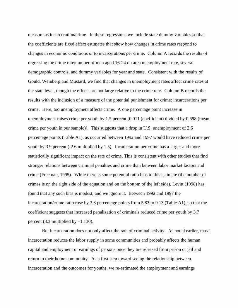
The most striking evidence in Figures 5 and 6 is the extent of incarceration among African

Americans. In both years and at all ages, African Americans have higher incarceration rates than

whites. In 1990 and 1996 non-Hispanic African Americans were about twice as likely as

Hispanics and nearly 8 times more likely than non-Hispanic whites to be in State or Federal

prison. At year-end 1996 there were 1,571 sentenced African American inmates per 100,000

African Americans in the United States, compared to 688 sentenced Hispanic inmates per

100,000 Hispanics and 193 white inmates per 100,000 whites. In 1996, 8.3 percent of African

American men age 25 to 29 were in prison compared to approximately 0.8 percent of white

males in the same age group. Even though incarceration rates fall with age, the share of African

American men age 45 to 54 in prison in 1996 was almost 3 percent. This value is more than 3

times the size of the highest rate of 0.9 percent among white men age 30 to 34. Based on 1980s

data the Justice Department estimates that 29 percent of all African American men will spend

time in prison (Bureau of Justice Statistics, 1997). The high rate of incarceration among African

American men has two effects on our data. First, it removes a substantial number of young

African American men from the CPS sample. Second, it implies that an increasing number of

African American men have a criminal record, which is likely to adversely affect their labor

market outcomes.

Turning from all men to the young less educated men of concern to this study, we have

calculated their employment and earnings during the periods 1983 to 1989 and 1992 to1998,

using the CPS files. Figures 7 and 8 (Appendix Table A2) shows that in the 1980s employment

rates among the non-college-educated rose but that their earnings fell. From 1992 to 1996 the

pattern is similar, though the increase in employment for the younger men is greater. But from

1996 to 1998, the picture is different. The employment for all non-college-educated men ceases

to grow, but their hourly earnings finally begin to increase, and hourly earnings increases most

markedly for young African American men.

The aggregate data thus suggest that in the 1990s the recovery of the economy from its low

point showed up first in employment and then, as unemployment fell to extremely low levels, in

wages. But these data do not have sufficient variation to allow us to characterize the effect of the

recovery to any greater extent. To determine further the effect of the boom on the less educated

young men, we turn to data on labor market conditions and outcomes across local labor markets.

For the 1990s we have 332 local labor markets, with a wide variety of unemployment

experiences, ranging from continuous low unemployment to rapid reductions in unemployment

to slow reductions in joblessness. These data provide us with market conditions that go beyond

the 1990s boom -- rates of unemployment below 4 percent in many areas -- that allow us to

assess what might happen to young workers if the aggregate economy produced even tighter

labor market conditions. Most important, it allows us to assess the effect of continued high

unemployment (below 4 percent for six ears of the expansion) on labor market outcomes and

thus to gain some insight as to the effects of a continuous or near continuous boom on these

workers.

Generalizing from patterns of change across areas to the nation as a whole has however,

some problems, because there are adjustments that occur across geographic areas that cannot

occur in the nation as a whole. In particular, migration across areas is a potentially important

response to different area economic conditions. Migration is likely to ameliorate the effects of

shocks on outcomes, as affected persons move from high to low unemployment locales. Still,

Topel (1986), Blanchflower, and Oswald (1999) and others find evidence that local labor

markets affect outcomes. And young non-college-educated workers are less mobile

geographically than other workers. Another important ameliorative effect is likely to occur

through product markets. In industries where prices are set nationally, a booming local market

will be unable to raise prices in response to increases in wages, which should produce a smaller

impact of low unemployment on wages than would be observed in a national boom. These and

other factors differentiate the labor market dynamics of a boom in local areas from that in the

entire economy, but do not gainsay the insight one can get from analyzing how local markets

respond to booms. In any case, area data are the only “game” in town with sufficient

observations to permit more than a description of events.

Area Variation

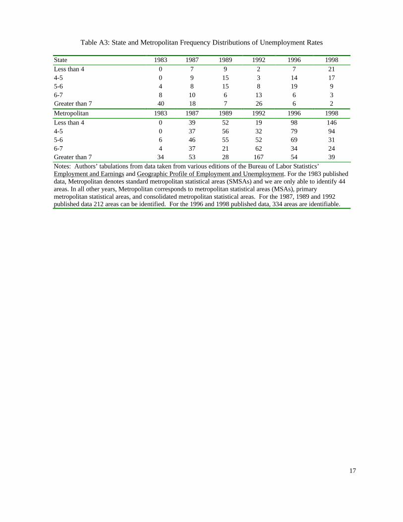
Figures 9 and 10 (Appendix Table A3) show the frequency distributions for the

unemployment rates by state and metropolitan area that are the key variables in our analysis.

Because the CPS identifies fewer metropolitan areas in 1983 than in later years, we report fewer

rates of area unemployment for the 1980s boom. Most areas begin the 1980s expansion with

unemployment rates that exceed 7 percent. By 1989 a sizeable number have unemployment rates

less than 5 percent. Most areas begin the 1990s boom with unemployment rates in the 6-7 or 7+

range. By 1996, over 98 metropolitan areas and 7 states have unemployment rates below 4

percent. Between January to July 1998 these figures jump to 146 metropolitan areas and 21

states.

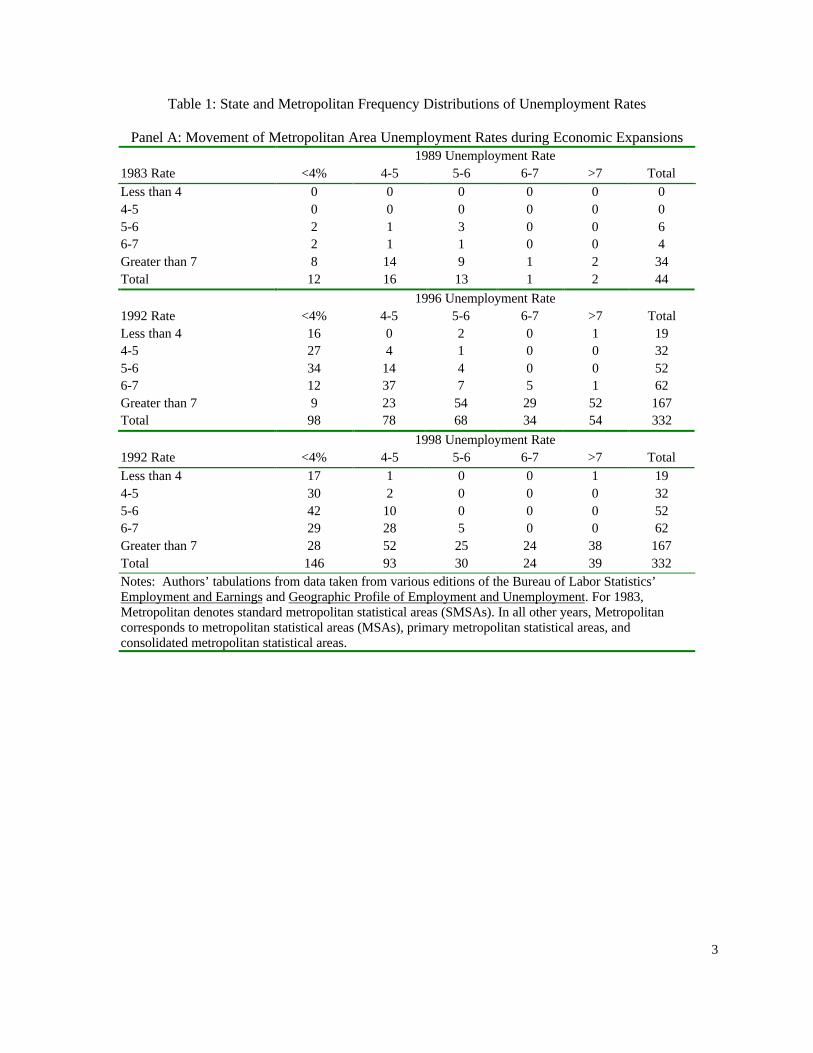
Panel A of Table 1 shows the transition matrix of metropolitan areas for the 1983 to 1989

and 1992 to 1998 periods. In both periods the matrix is near triangular with 0s dominating the

transitions to higher unemployment. During the 1980s boom no area moved from a lower

unemployment rate group to a higher unemployment rate group. In the 1990s boom just 2 areas

had 1998 unemployment rates above 1992 unemployment rates. Fifty-seven areas had

unemployment rates in the same group, while the vast majority of areas witness a decline in

unemployment. Of the 167 areas that started with unemployment rates greater than 7 percent, 80

have now moved into the less than 4 percent and 4-5 percent groups.

Panel B displays the transition probabilities associated with the 1990s boom. The areas that

started in the less than 4 percent group in 1992 remain in that group in 1998 with a very high

probability. From 1992 to 1996, 65 percent of 5-6 areas moved to the less than 4 percent

category, 60 percent of 6-7 areas moved to 4-5, and 63 percent of 7+ either moved to 5-6 or

remained at 7+. By 1998, 81 percent of 5-6 areas have moved to the less than 4percent category,

and 48 percent of 6-7 areas have moved to the less than 4 percent category. For the 7+ category,

almost 50 percent have moved to either the less than 4 or 4-5 percent category by 1998.

Overall, the reduction in unemployment is about 3 percentage points between 1992 to 1998,

but the table displays quite different histories among areas. To examine the various paths, we

focus on three types of areas: those with “continuous full employment” -- defined as areas with

unemployment rates below 4 percent in all years of the recovery (14 metro areas); those with

“steady high unemployment” -- defined as areas that had unemployment rates that exceeded 7

percent in all years (28 areas); and those with “rapid reductions in joblessness”, -- defined as

areas where unemployment rates fell by over 5 points (15 areas). More paths exist, but for

simplicity we focus on these cases.

Figure 11 plots the annual average unemployment rate for the three groups. The average for

areas with unemployment rates below 4 percent in all years is 3.2 percent in 1992 and falls to 2.0

percent in 1998. Table 2 shows the areas that experiences this continuous full employment.

They range from areas in Texas to midwestern metropolitan areas such as Des Moines and Iowa

City. The jobless rates for the group of areas with continuous high unemployment (rates in

excess of 7 percent) also fall, but the group average here remains in double digits: it drops from

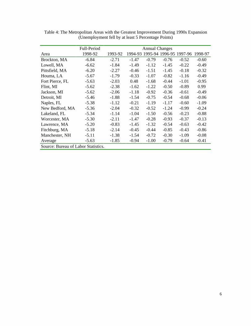
14.5 to 12.1 percent. Of these 28 areas, table3 shows that 11 are in California. Finally, areas with

reductions in unemployment rates in excess of 5 percentage points start at an average of 10.3

percent in 1992 and fall to 4.6 percent in 1998. Almost half of these metropolitan areas are

located in Massachusetts (see table 4).

Figure 12 shows the UCR crime rates for each of these groups in areas in the 1990s recovery

and in the preceding decade. Throughout the period the area with the worst unemployment

record have the highest rate of crime, while the areas with continuous low unemployment have a

low rate of crime. With the expansion, crime rates for the group with the largest drop in

unemployment falls the most, reaching essentially similar (in some years lower) levels in crime

as in areas with unemployment below 4 percent. These results offer one possible emendation to

the usual finding that unemployment is inversely related to crime: it suggests there is a limit to

the reduction in crime associated with low unemployment -- even 6 years of low unemployment

does not reduce the crime rate continuously. Rather, it simply keeps it at a lower than national

level.

Unemployment and Earnings and Employment

How much does the employment and earnings of non-college-educated men vary with

local labor market conditions?

To answer this question, we compared the economic positions of men across

metropolitan areas with different unemployment rates, using the micro CPS files. We used a

logit model for our employment analysis. The dependent variable is a 0-1 dummy variable for

whether the male is employed in a given year; the independent variables are the area

unemployment rate and measures of demographic characteristics: age, years of schooling and

race. The variable for race is a dummy variable that equals 1 if the respondent is African

American and 0 if the respondent is white. To estimate the wage effect, we regress the log

(natural log) of hourly earnings on the same variables used in the employment equations.

Tables 5 and 6 present our main results linking the employment and earnings of non-

college-educated young men to area unemployment rates and measures of crime, and

comparative analyses for all men (25-64). Although we have wage and employment information

for 1998, we do not have crime data for 1998. The results in Tables 5 and 6 are based on CPS

samples that exclude the 1998 data. We estimated models that excluded our measures of crime

and included the 1998 data, and summarize these results (which were similar to those in the

table) during our discussion. The column A regressions give results from cross section

regressions that exploit the differences among areas. The column B regressions give results from

regressions which include metropolitan area dummy variables: they show how changes in

unemployment in an area affect outcomes. We record both the estimated logit coefficients and

their effect on the probablities. The upper part of the table measures unemployment as a

continuous variable. The lower part divides unemployment rates by group, in an effort to find

any non-linearities.

Table 5 shows that area unemployment has a sizeable effect on the employment of young

non-college-educated men, both in the cross section and fixed effects specifications. In all of the

calculations the coefficients on unemployment for young workers exceed those for all men. For

instance the estimated effect of area unemployment on the probability of employment in the

cross section is -0.015 versus -0.009 for all men. In the fixed effects estimates in column B, the

estimated coefficients for the effect of unemployment on the employment of youths are generally

larger and diverge more from those for adults than in the cross section results. Within areas

changes in unemployment rates produce gains in employment for younger relative to older

workers. The largest logistic coefficient is for African American youths (-0.124) and the next

largest for all youths (-0.119), which compare to -0.074 for all men and -0.046 for African

American men. Given the different levels of employment for the groups, these figures translate

into larger gains in the probability of employment for younger African American youths than all

youths and similar gains in the probability of employment for older African American men and

older white men. In the bottom panel calculations in which we record coefficients on dummy

variables for particular levels of unemployment, there is relatively little evidence of any non-

linearities. These results do not change when the crime measures are excluded and the 1998 cross

section is added.

Table 6 records the estimated effects of unemployment on the natural logarithm of hourly

earnings, or the “wage curve” (Blanchflower and Oswald). Here, we find a striking difference

between the results for the young men and for the older men. In both the cross section and fixed

effects analysis, unemployment has a strong effect on the hourly pay of young men but has no

effect on the hourly earnings of 25-64 year old men. Unemployment has a slightly smaller effect

on the earnings of young African American men than on young white men (in contrast to

Freeman’s analysis of the 1983-87 period, which found a higher effect on young African

Americans). However, this result appears to occur because young African American men are in

areas that have taken longer for wages to rise. When we add the 1998 cross section (see

appendix A3) the unemployment coefficient for African American youth jumps from –0.019 to

-0.031, while the unemployment coefficient for all youth increases from –0.023 to –0.024. The

gains for African American youth occur in the less than 4 percent, 4-5 and 5-6 categories.

Indeed, the coefficients shown in Table 6 all increase by about 0.03 points when the 1998 cross

section is added, which implies that the effect of the boom on earnings increased substantially in

the 1996-1998 period. One reason may be that it takes time for the boom to raise demand and

eventually the pay for African American youths.

Turning to the bottom part of the table, we find some evidence of non-linear effects of

unemployment on the log earnings of young workers. In areas with unemployment below four

percent, the fixed effects (column B) estimates show that the earnings of young non-college-

educated men are 0.121 points higher, whereas they are just 0.018 points higher for all non-

college-educated men. The coefficients on areas with 4-5% unemployment and areas with less

than 4% unemployment differ by .04 points for the young men, but differ by only .008 points for

all men. The implication is that very tight labor markets may improve the earnings of young

non-college-educated workers without creating overall wage inflation.

In addition to unemployment, the regressions in tables 5 and 6 contain one area variable

that is not normally part of wage curves-- the rate of crime per young person in the state. We

have included it because of the substantial number of young men, particularly African American

men, involved in crime and because of the likelihood that their criminal activity will affect labor

market outcomes. Youths engaged in crime are likely to participate less in the local labor

market, reducing the youth supply, and may have lower human capital than otherwise

comparable youths, reducing their skills as well. In the fixed effects regressions, the coefficient

on crime is negative in nearly all cases, implying that in areas where crime rose, employment fell

and earnings fell. As we have controlled for area unemployment, one interpretation of this

relation is that conditional on the labor market, youths in areas with more crime are trading jobs

or legitimate earnings for criminal activity. If this were correct, we would expect that the

coefficients on crime in the regressions for African-Americans (for whom crime is a more

common choice) to be larger than those in the regressions for all men, and indeed this is true in

the calculations. But we would also expect the crime coefficients in the young male regressions

to exceed those for all men, and this is not the case. As our crime data are for states and our

unemployment data are for areas within states, we are not prepared to make too much of this

pattern.

Finally, in Table 7 we examine the time pattern of the effect of unemployment on

employment and earnings in greater depth by including the unemployment rate at the boom’s

beginning -- the trough unemployment -- to the regressions for earnings and employment. Panel

A shows the effect of area unemployment on employment, including the trough unemployment

rate. Panel B shows the effect of area unemployment on earnings, including the trough

unemployment rate. The trough unemployment rate enters most of the regressions with a

substantial effect that magnifies the estimated impact of a tight market on youth employment and

earnings and increases the differential effect of the labor market on youths as opposed to adults.

At the same level of unemployment, a higher trough unemployment rate implies lower

employment and earnings for youths; whereas it has only a modest effect for adults. One

interpretation is that this is a kind of hysterisis, where the past has an independent effect on

young workers, perhaps because it impacts the school-to-work transition. The wages and

employment of youths may be determined by a dynamic adjustment process, with some lags, so

that focusing solely on the current years’ area unemployment as the key independent variable in

the analysis is incorrect. Perhaps a Phillips curve type specification is more appropriate than the

standard wage curve (Blanchard and Katz, 1999).

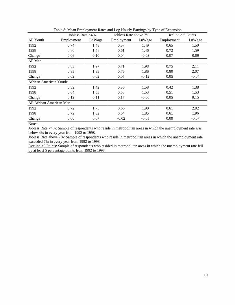
To examine the pattern of change in employment and wages across areas with different

unemployment histories, we have tabulated in Table 8 the outcome variables for less educated

men in the three types of areas that we specified earlier: continuous full employment areas

(jobless rates below 4 percent in all years); steady high unemployment (jobless rates that exceed

7 percent in all years), and areas of rapid improvement where jobless rates fell by at least 5

percentage points. On the employment side, what is striking is the sizeable increase in

employment for young workers relative to older workers in the tightest labor markets and labor

markets with the biggest declines in unemployment. The data for all youths show roughly similar

gains in employment across the areas in percentage points (from different starting points). From

1992 to 1998, the gains are 6 points in the continuous full employment areas, 4 points in the high

unemployment areas, and 7 points in the rapidly improving areas. All men also have roughly

similar gains in employment, but these are relatively modest. By 1998 the young less educated

in the continuous full employment areas have rates of employment that actually exceed the

employment rates for the older less educated men in the continuous high unemployment areas.

All youths in these areas have roughly 80 percent employment rates! The increases in

employment rates for less educated young African American men, which are largest in the

continuous full employment local labor markets, close a substantial portion of the gap between

them and similarly educated young white men. The implication is that a long extended boom

can go a long way to resolving the African American youth employment problem.

The pattern of change in the earnings across areas tells a similar story: larger gains for the

young less educated men than for older less educated men, though here young African American

less educated men do no better than other less educated young men. One possible reason for the

absence of any particular wage effect in the continuous high employment areas is that initially in

1992 the wages of young less educated are reasonably close to that of all less educated youth

(1.42 vs 1.48 for a 6 ln point difference). This may in part be due to the minimum wage, which

tends to compress wages at the bottom of the earnings distribution.

All told, table 8 suggests that the economic boom of the 1990s substantially improved the

job market for less educated young men, including young African Americans, and that

continuous full employment has the potential for creating full employment and rising wages for

these workers. By contrast, the gains for all less educated men are more modest.

Is the Wage Gain Due to Full Employment or the Minimum Wage?

In 1996, the federal minimum wage increased from $4.25 to $4.75. In 1997, it increased

from $4.75 to $5.15. As these changes undoubtedly affected the wages of less educated workers,

they are a confounding factor in the estimates of the effect of area unemployment on earnings.

One possibility is that at any given unemployment rate, earnings in areas where the minimum

wage had greater impact will be higher for young less educated men than in areas where the

minimum wage had a smaller impact, and correspondingly employment may less. This will bias

our estimates of area effects if there is a correlation between the minimum wage and the level or

change in area unemployment. One possibility is that the minimum wage raised wages in areas

with high unemployment or areas where unemployment fell modestly, which would bias

downward our estimate of the impact of area conditions on unemployment. But if the minimum

wage induced increases in wages lowered employment, our estimates of the effect of area

unemployment on employment would be biased upward. We attribute too much of the

employment gains of less-educated in areas of low or declining unemployment to the economic

expansion, by ignoring the fact that in those areas the minimum was not as binding as in areas

with high unemployment or more modestly declining unemployment.

Table 9 examines whether the federal minimum wage hikes in 1996 and 1997 bias our

estimates of the relationship between area unemployment and the employment and earnings of

men. To test for this possibility, we sorted the CPS sample into two groups. The first are

respondents that live in states where the federal minimum wage hikes of 1996 and 1997 were

binding. These are states in which the federal minimum wage exceeded the state's minimum

wage. The second group is comprised of respondents that live in states where the federal

minimum wage hikes were not binding. The federal increases remained at or below the state

minimum wage. Table A4 displays the federal and state minimum wages and the ratios used to

create the groups.

To model the impact, we added two new variables to our earlier models: a dummy

variable that equals 1 if the respondent lives in a state where the hikes were binding, and 0 if they

were not binding; and interaction between the binding dummy variable and the area

unemployment rate. It is the coefficient on the interaction term that is most relevant to our

analysis. The evidence in Table 9 suggests that the minimum wage hikes of 1996 and 1997 do

not bias our results. The interaction terms are basically zero in both the employment and

earnings equations. The coefficient on the binding dummy is nonzero, but generally statistically

insignificant, with no distinct pattern.3

The Relation Between Outcomes and Crime

We examine the relation between crime and labor market conditions and outcomes in two

ways. First, in Table 10 we estimate a standard supply of crime equation in which we relate the

crime per youth in a given state to unemployment and a measure of the potential disincentive

effect of criminal punishment or risk of getting caught and penalized severely. We define our

measure as incarceration/crime. In these regressions we include state dummy variables so that

the coefficients are fixed effect estimates that show how changes in crime rates respond to

changes in economic conditions or to incarcerations per crime. Column A records the results of

regressing the crime rate/number of men aged 16-24 on area unemployment rate, several

demographic controls, and dummy variables for year and state. Consistent with the results of

Gould, Weinberg and Mustard, we find that changes in unemployment rates affect crime rates at

the state level, though the effects are not large relative to the crime rate. Column B records the

results with the inclusion of a measure of the potential punishment for crime: incarcerations per

crime. Here, too unemployment affects crime. A one percentage point increase in

unemployment raises crime per youth by 1.5 percent [0.011 (coefficient) divided by 0.698 (mean

crime per youth in our sample)]. This suggests that a drop in U.S. unemployment of 2.6

percentage points (Table A1), as occurred between 1992 and 1997 would have reduced crime per

youth by 3.9 percent (-2.6 multiplied by 1.5). Incarceration per crime has a larger and more

statistically significant impact on the rate of crime. This is consistent with other studies that find

stronger relations between criminal penalties and crime than between labor market factors and

crime (Freeman, 1995). While there is some potential ratio bias to this estimate (the number of

crimes is on the right side of the equation and on the bottom of the left side), Levitt (1998) has

found that any such bias is modest, and we ignore it. Between 1992 and 1997 the

incarceration/crime ratio rose by 3.3 percentage points from 5.83 to 9.13 (Table A1), so that the

coefficient suggests that increased penalization of criminals reduced crime per youth by 3.7

percent (3.3 multiplied by –1.130).

But incarceration does not only affect the rate of criminal activity. As noted earlier, mass

incarceration reduces the labor supply in some communities and probably affects the human

capital and employment or earnings of persons once they are released from prison or jail and

return to their home community. As a first step toward seeing the relationship between

incarceration and the outcomes for youths, we re-estimated the employment and earnings

equations in tables 5 and 6 by replacing the crimes per young man variable with incarcerations

per young man. As the unemployment rate coefficients are unaffected by this, we report in Table

11 simply the coefficient on incarcerations/crime. It is strong and negative in the fixed effects

regressions in columns B though not in the cross-section calculations in columns A for youths

and for adults. The coefficients are especially large in the earnings equations for African

American young and all men. Areas with the most rapidly rising rates of incarceration are areas

in which youths, particularly, African American youths have had the worst earnings and

employment experience, and where men aged 25-64 have also done poorly. Whether this

association is due to the depressing effect of criminal records on labor market outcomes cannot

be ascertained from the aggregate data.

Conclusion

The US economy has experienced nine post-World War II expansions.4 The current

expansion, which started in March 1991, and continues as of this writing, March 1999, has

shattered the length of the previous longest peace-time boom from November 1982 to July 1990

expansion. The national unemployment rate started at 6.8 percent and currently sits at 4.3

percent. The unemployment rates in many metropolitan areas sit well below 4 percent. In 1998,

44 percent of metropolitan unemployment rates were below four percent, implying that roughly

half of the US was enjoying extremely tight labor markets.

The NAIRU has seemingly shifted, as low rates of unemployment have not generated the

same increases in wages as in previous economic booms. If the boom of the late 1990’s was

insufficient to improve substantially the position of young non-college-educated workers, it is

difficult to imagine that any expansion could do so, and thus would dash any hope that economic

growth per se could raise their pay and income. Our analysis has shown that the 1990s boom has

substantially improved the labor market outcomes of young non-college-educated men; and

helped the young African American men who are the most disadvantaged and socially troubled

group in the U.S.. Young men in tight labor markets in the 1990s experienced a noticeable boost

Figure 3:

Figure 4:

Average Real Hourly Earnings ($1998)Private Nonagricultural Workers

Source: Bureau of Labor Statistics.

$13.14

$12.90

$12.71

$12.30 $12.29$12.43

$12.77

1983 1987 1989 1992 1996 1997 1998$12.00

$12.50

$13.00

$13.50

$14.00

Crime and Incarceration Rates per 100,000

Source: Selected Volumes of the Unif orm Crime Reports.

5159

55505741 5660

50794876

179

228

271

330

427445

1983 1987 1989 1992 1996 19974000

4500

5000

5500

6000

6500

7000

0

100

200

300

400

500

Crime Rate per 100,000 Incarceration Rate per 100,000

Figure 5:

Figure 6:

Growth in Incarceration Rate per 100,000(1996 - 1990)

53

111

88

133

167

126

61

12

253

10891182

1031

1425

998

757

50

18-19 20-24 25-29 30-34 35-39 40-44 45-54 55+0

200

400

600

800

1000

1200

1400

1600

0

50

100

150

200

White African American

1996 Incarceration Rate per 100,000by Race and Age

Source: Unif orm Crime Reports and Sourcebook on Criminal Justice Statistics.

0.1430.406 0.442 0.469 0.412 0.322

0.1980.044

1.337

3.385

4.131

3.6713.398

2.431

1.347

0.218

18-19 20-24 25-29 30-34 35-39 40-44 45-54 55+0

1

2

3

4

5

White African American

Figure 7:

Figure 8:

Real Earnings of Less-Educated Menby Race and Age

Source: Authors' calculations f rom CPS.

2.162.08

2.031.96 1.96

2.02

1.881.84

1.79 1.81

1.631.56

1.50 1.471.531.51

1.44 1.421.34

1.45

1983 1989 1992 1996 19981.00

1.20

1.40

1.60

1.80

2.00

2.20

2.40

Adult White Adult African American

Youth White Youth African American

Employment Population Ratios of Less-Educated Men

by Race and Age

Source: Authors' calculations f rom CPS.

7781 79

82 83

6568

65 66 6873

7773

77 77

44

57

4649

54

1983 1989 1992 1996 199830

40

50

60

70

80

90

100

Adult White Adult African American

Youth White Youth African American

1

Figure 9:

Figure 10:

State Frequency Distributions of Unemployment Rates

Source: Authors' tabulations f rom BLS.

0

9

2

7

21

0

15

3

1417

4

15

8

19

986

13

63

40

7

26

6

2

1983 1989 1992 1996 19980

10

20

30

40

50

Less than 4% 4-5 5-6 6-7 Greater than 7

Metropolitan Area Frequency Distributions of Unemployment Rates

Source: Authors' tabulations f rom BLS.

0

52

19

98

146

0

56

32

79

94

6

55 52

69

31

4

21

62

3424

3428

167

54

39

1983 1989 1992 1996 19980

50

100

150

200

Less than 4% 4-5 5-6 6-7 Greater than 7

2

Figure 11:

Figure 12:

Area Unemployment ComparisonsGroup Averages

Source: Bureau of Labor Statistics

3.2 3.0 2.8 2.5 2.6 2.2 2.0

14.5 14.3

13.2 12.9 12.611.8 12.1

10.3

8.47.5

6.55.7

5.0 4.6

1992 1993 1994 1995 1996 1997 19980.0

2.0

4.0

6.0

8.0

10.0

12.0

14.0

16.0

Top Worst Best Improvement

MSA Crime Rates per 100,000 Inhabitantsby Type of Recovery in Unemployment

Source: Authors' tabulations from assorted years of Crime in the United States.

1983 1987 1989 1992 1993 1994 1995 1996 19970.0

2.0

4.0

6.0

8.0

Worst Biggest Decline Top

Worst: Unemployment Rate >7% in all Years

Biggest Decline in Unemployment

Top Unemployment Rate <4% in all Years

3

Table 1: State and Metropolitan Frequency Distributions of Unemployment Rates

Panel A: Movement of Metropolitan Area Unemployment Rates during Economic Expansions1989 Unemployment Rate

1983 Rate <4% 4-5 5-6 6-7 >7 TotalLess than 4 0 0 0 0 0 04-5 0 0 0 0 0 05-6 2 1 3 0 0 66-7 2 1 1 0 0 4Greater than 7 8 14 9 1 2 34Total 12 16 13 1 2 44

1996 Unemployment Rate1992 Rate <4% 4-5 5-6 6-7 >7 TotalLess than 4 16 0 2 0 1 194-5 27 4 1 0 0 325-6 34 14 4 0 0 526-7 12 37 7 5 1 62Greater than 7 9 23 54 29 52 167Total 98 78 68 34 54 332

1998 Unemployment Rate1992 Rate <4% 4-5 5-6 6-7 >7 TotalLess than 4 17 1 0 0 1 194-5 30 2 0 0 0 325-6 42 10 0 0 0 526-7 29 28 5 0 0 62Greater than 7 28 52 25 24 38 167Total 146 93 30 24 39 332Notes: Authors’ tabulations from data taken from various editions of the Bureau of Labor Statistics’Employment and Earnings and Geographic Profile of Employment and Unemployment. For 1983,Metropolitan denotes standard metropolitan statistical areas (SMSAs). In all other years, Metropolitancorresponds to metropolitan statistical areas (MSAs), primary metropolitan statistical areas, andconsolidated metropolitan statistical areas.

4

Table 1 cont: State and Metropolitan Frequency Distributions of Unemployment Rates

Panel B: Metropolitan Area Transition Probabilities1996 Unemployment Rate

1992 Rate <4% 4-5 5-6 6-7 >7 Total

<4% 0.84 0.00 0.11 0.00 0.05 1.004-5 0.84 0.13 0.03 0.00 0.00 1.005-6 0.65 0.27 0.08 0.00 0.00 1.006-7 0.19 0.60 0.11 0.08 0.02 1.00>7 0.05 0.14 0.32 0.17 0.31 1.00Total 0.30 0.23 0.20 0.10 0.16 1.00

1998 Unemployment Rate1992 Rate <4% 4-5 5-6 6-7 >7 Total

<4% 0.89 0.05 0.00 0.00 0.05 1.004-5 0.94 0.06 0.00 0.00 0.00 1.005-6 0.81 0.19 0.00 0.00 0.00 1.006-7 0.47 0.45 0.08 0.00 0.00 1.00>7 0.17 0.31 0.15 0.14 0.23 1.00Total 0.44 0.28 0.09 0.07 0.12 1.00Notes: Authors’ tabulations from data taken from various editions of the Bureau ofLabor Statistics’ Employment and Earnings and Geographic Profile of Employmentand Unemployment. Each entry represents the probability of 1996 (1998)unemployment conditional on 1992 Unemployment.

Table 2: The Top Metropolitan Areas During the 1990s Expansion(Unemployment has remained Less than 4% in every year)

Area 1992 1993 1994 1995 1996 1997 1998Bryan, TX 2.9 2.7 2.7 3.0 2.5 2.2 1.8Columbia, MO 2.5 3.2 2.0 1.9 1.7 1.6 1.7Des Moines, IA 3.7 3.4 2.8 2.6 2.8 2.4 2.1Fargo, ND-MN 3.6 3.1 2.7 2.6 2.5 1.8 1.5Fayetteville, AR 3.7 2.9 2.5 2.4 2.9 3.1 3.4Iowa City, IA 3.3 2.7 2.6 2.7 2.9 2.4 2.1Lafayette, IN 3.8 3.4 3.5 3.1 2.8 2.4 2.3Lincoln, NE 2.7 2.3 2.4 2.3 2.6 1.8 1.6Madison, WI 2.2 2.2 2.3 1.8 1.7 1.7 1.6Omaha, NE-IA 3.6 3.1 3.2 2.8 3.0 2.5 2.1Raleigh-Durham-Chapel Hill, NC 3.8 3.1 2.7 2.6 2.4 2.0 1.9Rapid City, SD 3.2 3.8 3.4 3.0 3.3 2.7 2.7Rochester, MN 3.0 3.3 3.5 2.9 3.0 2.1 1.8Sioux Falls, SD 2.4 2.5 2.4 2.0 2.1 1.8 1.7Average 3.2 3.0 2.8 2.5 2.6 2.2 2.0Source: Bureau of Labor Statistics.

5

Table 3: The Worst Metropolitan Areas During the 1990s Expansion(Unemployment has remained above 7% in every year)

Area 1992 1993 1994 1995 1996 1997 1998Atlantic-Cape May, NJ 11.1 10.4 9.9 9.6 9.4 8.6 9.5Bakersfield, CA 15.5 15.8 14.7 13.8 12.7 11.8 12.6Beaumont, TX 9.3 11.4 10.1 9.8 9.1 8.0 7.2Brownsville, TX 14.7 13.5 12.8 12.6 12.6 12.5 12.7Chico-Paradise, CA 11.7 11.9 10.2 10.0 9.0 8.7 9.2Cumberland, MD-WV 12.4 10.6 8.8 8.6 8.0 7.9 8.0El Paso, TX 11.7 10.8 10.4 10.5 11.6 11.1 10.0Fort Pierce, FL 13.9 11.9 12.4 10.7 10.2 9.2 8.3Fresno, CA 15.9 15.5 14.0 14.3 13.2 13.5 14.8Jersey City, NJ 11.2 10.0 9.3 9.3 9.2 8.0 8.0Laredo, TX 11.0 10.5 9.6 15.4 12.7 10.5 9.5Las Cruces, NM 7.8 8.5 8.6 8.6 10.2 8.4 9.7McAllen, TX 22.3 20.6 19.5 19.8 18.9 18.1 17.5Merced, CA 16.5 17.1 15.6 16.9 16.2 15.2 17.1Modesto, CA 16.5 16.7 15.7 15.3 14.1 13.1 13.4New Bedford, MA 12.7 10.6 10.3 9.8 8.5 7.5 7.3New York, NY 10.2 9.6 8.1 7.6 8.0 8.4 7.6Pine Bluff, AR 11.4 9.5 8.8 7.6 7.7 7.5 8.0Redding, CA 13.2 12.6 11.9 11.3 9.9 9.1 10.0Salinas, CA 12.4 12.9 12.1 12.5 11.1 10.7 12.2Santa Cruz, CA 9.8 10.4 9.7 9.2 8.3 7.6 7.9Stockton-Lodi, CA 14.0 14.0 12.6 12.3 11.2 10.7 11.5Texarkana, TX-AR 9.0 8.6 9.2 7.9 7.4 7.4 7.5Vineland, NJ 12.1 11.3 10.5 9.7 9.9 8.9 10.0Visalia, CA 16.6 17.9 16.0 16.6 15.9 15.3 16.1Yakima, WA 13.8 14.6 11.8 12.7 13.6 10.2 10.6Yuba City, CA 18.2 18.6 16.2 16.3 15.1 14.4 16.7Yuma, AZ 26.5 27.6 31.5 28.2 30.5 26.7 25.3Average 14.5 14.3 13.2 12.9 12.6 11.8 12.1Source: Bureau of Labor Statistics.

6

Table 4: The Metropolitan Areas with the Greatest Improvement During 1990s Expansion(Unemployment fell by at least 5 Percentage Points)

Full-Period Annual ChangesArea 1998-92 1993-92 1994-93 1995-94 1996-95 1997-96 1998-97Brockton, MA -6.84 -2.71 -1.47 -0.79 -0.76 -0.52 -0.60Lowell, MA -6.62 -1.84 -1.49 -1.12 -1.45 -0.22 -0.49Pittsfield, MA -6.20 -2.27 -0.46 -1.51 -1.45 -0.18 -0.32Houma, LA -5.67 -1.79 -0.33 -1.07 -0.82 -1.16 -0.49Fort Pierce, FL -5.63 -2.03 0.48 -1.68 -0.44 -1.01 -0.95Flint, MI -5.62 -2.38 -1.62 -1.22 -0.50 -0.89 0.99Jackson, MI -5.62 -2.06 -1.18 -0.92 -0.36 -0.61 -0.49Detroit, MI -5.46 -1.88 -1.54 -0.75 -0.54 -0.68 -0.06Naples, FL -5.38 -1.12 -0.21 -1.19 -1.17 -0.60 -1.09New Bedford, MA -5.36 -2.04 -0.32 -0.52 -1.24 -0.99 -0.24Lakeland, FL -5.34 -1.14 -1.04 -1.50 -0.56 -0.23 -0.88Worcester, MA -5.30 -2.11 -1.47 -0.28 -0.93 -0.37 -0.13Lawrence, MA -5.20 -0.83 -1.45 -1.32 -0.54 -0.63 -0.42Fitchburg, MA -5.18 -2.14 -0.45 -0.44 -0.85 -0.43 -0.86Manchester, NH -5.11 -1.38 -1.54 -0.72 -0.30 -1.09 -0.08Average -5.63 -1.85 -0.94 -1.00 -0.79 -0.64 -0.41Source: Bureau of Labor Statistics.

7

Table 5: The Effect of Area Unemployment Rates on the Employment of MenAll Youths All Men African American Youths African American Men

A B A B A B A BItem Coef. dP/dX Coef. dP/dX Coef. dP/dX Coef. dP/dX Coef. dP/dX Coef. dP/dX Coef. dP/dX Coef. dP/dX

Unemployment Rate -0.078 -0.015 -0.119 -0.023 -0.058 -0.009 -0.074 -0.012 -0.144 -0.035 -0.124 -0.030 -0.081 -0.017 -0.046 -0.010(0.007) (0.001) (0.015) (0.003) (0.004) (0.001) (0.008) (0.001) (0.020) (0.005) (0.039) (0.009) (0.010) (0.002) (0.019) (0.004)

African American -1.028 -0.194 -1.061 -0.201 -0.743 -0.120 -0.779 -0.126(0.037) (0.007) (0.041) (0.008) (0.020) (0.003) (0.022) (0.004)

Crime per Youth 0.081 0.015 -0.284 -0.054 -0.018 -0.003 -0.447 -0.073 0.269 0.066 -0.466 -0.114 0.013 0.003 -0.768 -0.164(0.072) (0.014) (0.190) (0.036) (0.036) (0.006) (0.093) (0.015) (0.146) (0.036) (0.338) (0.083) (0.068) (0.015) (0.155) (0.033)

Log Likelihood -14369 -14094 -56152 -55581 -2586 -2406 -9735 -9406

Less than 4% 0.521 0.099 0.425 0.080 0.443 0.072 0.360 0.058 0.839 0.205 0.133 0.133 0.529 0.112 0.077 0.077(0.050) (0.010) (0.084) (0.016) (0.026) (0.004) (0.042) (0.007) (0.115) (0.028) (0.051) (0.051) (0.057) (0.012) (0.022) (0.022)

4-5 0.436 0.083 0.397 0.075 0.304 0.049 0.243 0.039 0.564 0.138 0.092 0.092 0.315 0.067 0.027 0.027(0.049) (0.009) (0.070) (0.013) (0.025) (0.004) (0.034) (0.006) (0.115) (0.028) (0.041) (0.041) (0.061) (0.013) (0.018) (0.018)

5-6 0.268 0.051 0.280 0.053 0.235 0.038 0.199 0.032 0.321 0.078 0.068 0.068 0.281 0.060 0.034 0.034(0.044) (0.008) (0.059) (0.011) (0.023) (0.004) (0.029) (0.005) (0.099) (0.024) (0.033) (0.033) (0.051) (0.011) (0.014) (0.014)

6-7 0.223 0.042 0.172 0.033 0.171 0.028 0.123 0.020 0.290 0.071 0.030 0.030 0.336 0.072 0.048 0.048(0.050) (0.009) (0.065) (0.012) (0.026) (0.004) (0.033) (0.005) (0.117) (0.028) (0.038) (0.038) (0.063) (0.013) (0.017) (0.017)

African American -1.016 -0.192 -1.058 -0.200 -0.741 -0.120 -0.779 -0.126(0.037) (0.007) (0.041) (0.008) (0.020) (0.003) (0.022) (0.004)

Crime per Youth 0.097 0.018 -0.359 -0.068 0.000 0.000 -0.464 -0.075 0.231 0.056 -0.137 -0.137 -0.016 -0.003 -0.170 -0.170(0.073) 0.014 (0.192) 0.036 (0.037) 0.006 (0.093) 0.015 (0.149) (0.036) (0.083) (0.083) (0.070) 0.015 (0.033) (0.033)

Log Likelihood -14368 -14107 -56120 -55588 -2583 -2407 -9725 -9401

Notes: Calculated from the Current Population Survey Annual Merged Outgoing Rotation Group files, 1987, 1989, 1992 and 1996. The entries are logit coefficients,followed by the probability effect (logit coefficients multiplied by p*(1-p), where p is the share of the sample that are employed). All logit models include yeardummy variables, age, age squared, years of schooling dummy variables, and a race dummy variable. Standard errors are in parentheses. Column A excludes MSAdummy variables. Column B includes MSA dummy variables. We also estimated models where we exclude crimes per youth and include the 1998 cross section. Weare forced to do this because the 1998 crime rates are not available. The coefficients from the linear specifications that include the MSA dummy variables are -0.023(0.003) for all youth, -0.011 (0.001) for all men, -0.027 (0.008) for African American youth and -0.010 (0.004) for African American men. Standard errors are inparentheses.

8

Table 6: Effect of Area Unemployment Rates on the Earnings of Men

All Youths All MenAfrican American

YouthsAll African

American MenItem A B A B A B A B

Unemployment Rate -0.018 -0.023 -0.003 -0.001 -0.020 -0.019 0.006 -0.001(0.001) (0.003) (0.001) (0.002) (0.004) (0.008) (0.003) (0.005)

African American -0.136 -0.146 -0.184 -0.195(0.008) (0.009) (0.005) (0.005)

Crime per Youth -0.011 -0.098 -0.045 -0.070 0.082 -0.148 0.012 -0.056(0.013) (0.032) (0.008) (0.020) (0.029) (0.067) (0.017) (0.040)

R2 0.202 0.198 0.145 0.144 0.138 0.111 0.088 0.085

Less than 4% 0.125 0.121 -0.005 0.018 0.110 0.059 -0.032 0.001(0.009) (0.014) (0.006) (0.009) (0.025) (0.045) (0.015) (0.026)

4-5 0.068 0.081 -0.010 0.010 0.071 0.051 -0.026 0.003(0.009) (0.012) (0.006) (0.007) (0.026) (0.037) (0.016) (0.021)

5-6 0.049 0.074 -0.020 0.010 0.046 0.041 -0.061 -0.008(0.008) (0.011) (0.005) (0.006) (0.023) (0.031) (0.014) (0.018)

6-7 0.010 0.038 -0.027 0.006 0.016 0.046 -0.038 0.031(0.009) (0.012) (0.006) (0.007) (0.027) (0.035) (0.016) (0.020)

African American -0.136 -0.146 -0.183 -0.195(0.008) (0.009) (0.005) (0.005)

Crime per Youth 0.000 -0.099 -0.051 -0.067 0.078 -0.165 0.014 -0.059(0.013) (0.032) (0.008) (0.020) (0.029) (0.066) (0.017) (0.039)

R2 0.204 0.200 0.145 0.144 0.139 0.106 0.090 0.085Sample Size 18607 18607 73294 73294 2088 2088 9499 9499

Notes: Calculated from the Current Population Survey Annual Merged Outgoing Rotation Group files, 1987,1989, 1992 and 1996. All regressions include year dummy variables, age, age squared, years of schoolingdummy variables, and a race dummy variable. Standard errors are in parentheses. Column A excludes MSAdummy variables. Column B includes MSA dummy variables. We also estimated models where we excludecrimes per youth and include the 1998 cross section. We are forced to do this because the 1998 crime ratesare not available. The coefficients from the linear specifications that include the MSA dummy variables are -0.024 (0.002) for all youth, -0.002 (0.002) for all men, -0.031 (0.007) for African American youth, and -0.004 (0.004) for African American men. Standard errors are in parentheses.

9

Table 7: The Effect of Current and Past Unemployment on Earnings and EmploymentPanel A: Employment

Young Adults All Men Young African American Men African American MenA B A B A B A B

Item Coef. DP/dX Coef. dP/dX Coef. dP/dX Coef. dP/dX Coef. dP/dX Coef. dP/dX Coef. dP/dX Coef. dP/dXUnemployment Rate -0.041 -0.007 -0.047 -0.008 0.007 0.001 -0.092 -0.014 -0.130 -0.029 -0.069 -0.016 -0.004 -0.001 -0.103 -0.021

(0.022) (0.004) (0.046) (0.008) (0.011) (0.002) (0.023) (0.003) (0.055) (0.013) (0.097) (0.022) (0.028) (0.006) (0.053) (0.011)Trough Unemployment Rate -0.045 -0.007 -0.096 -0.016 -0.051 -0.008 0.013 0.002 -0.070 -0.016 -0.154 -0.035 -0.080 -0.016 0.046 0.009

(0.018) (0.003) (0.040) (0.007) (0.010) (0.001) (0.019) (0.003) (0.040) (0.009) (0.083) (0.019) (0.021) (0.004) (0.047) (0.009)African American -0.980 -0.164 -1.008 -0.168 -0.778 -0.116 -0.781 -0.117

(0.065) (0.011) (0.071) (0.012) (0.034) (0.005) (0.036) (0.005)Crime per Youth -0.044 -0.007 -0.437 -0.073 -0.022 -0.003 -0.605 -0.091 0.123 0.028 -0.621 -0.141 -0.141 -0.029 -0.816 -0.166

(0.133) (0.022) (0.290) (0.048) (0.061) (0.009) (0.140) (0.021) (0.234) (0.053) (0.462) (0.105) (0.097) (0.020) (0.195) (0.040)Log Likelihood -4332 -4179 -19119 -18858 -932 -830 -3827 -3663Notes: Calculated from the Current Population Survey Annual Merged Outgoing Rotation Group files, 1989 and 1996. The entries are logit coefficients, followed by the probability effect(logit coefficients multiplied by p*(1-p), where p is the share of the sample that are employed). All logit models include variables for age, age squared, years of schooling, and race.Unemployment rate refers to the 1996 and 1989 rates, while trough unemployment rate refers to the 1983 and 1992 rates. Column A excludes MSA dummy variables. Column B includesMSA dummy variables. Standard errors are in parentheses.

Panel B: Earnings Young Adults All Men Young African American Men African American Men

Item A B A B A B A B

Unemployment rate -0.011 -0.021 -0.021 -0.011 -0.012 -0.020 -0.023 -0.016

(0.004) (0.007) (0.002) (0.005) (0.011) (0.020) (0.007) (0.013)

Trough Unemployment Rate -0.011 -0.032 0.011 -0.007 -0.003 -0.017 0.020 0.003

(0.003) (0.006) (0.002) (0.004) (0.008) (0.017) (0.005) (0.011)

African American -0.154 -0.163 -0.162 -0.172

(0.013) (0.014) (0.008) (0.008)

Crime per Youth -0.028 -0.016 -0.055 -0.032 0.055 -0.012 0.037 0.016

(0.022) (0.047) (0.014) (0.030) (0.038) (0.074) (0.025) (0.048)

R2 0.210 0.188 0.173 0.168 0.209 0.189 0.123 0.117

Sample Size 5796 5796 22562 22562 764 764 3388 3388

Notes: Calculated from the Current Population Survey annual merged files, 1989 and 1996. All regressions include variables for age, agesquared, years of schooling, and race. Unemployment rate refers to the 1996 and 1989 rates, while trough unemployment rate refers to the 1983and 1992 rates. Column A excludes MSA dummy variables. Column B includes MSA dummy variables. Standard errors are in parentheses.

10

Table 8: Mean Employment Rates and Log Hourly Earnings by Type of ExpansionJobless Rate <4% Jobless Rate above 7% Decline > 5 Points

All Youth Employment LnWage Employment LnWage Employment LnWage1992 0.74 1.48 0.57 1.49 0.65 1.501998 0.80 1.58 0.61 1.46 0.72 1.59Change 0.06 0.10 0.04 -0.03 0.07 0.09All Men

1992 0.83 1.97 0.71 1.98 0.75 2.111998 0.85 1.99 0.76 1.86 0.80 2.07Change 0.02 0.02 0.05 -0.12 0.05 -0.04

African American Youths

1992 0.52 1.42 0.36 1.58 0.42 1.381998 0.64 1.53 0.53 1.53 0.51 1.53Change 0.12 0.11 0.17 -0.06 0.05 0.15All African American Men

1992 0.72 1.75 0.66 1.90 0.61 2.021998 0.72 1.82 0.64 1.85 0.61 1.96Change 0.00 0.07 -0.02 -0.05 0.00 -0.07Notes:Jobless Rate <4%: Sample of respondents who reside in metropolitan areas in which the unemployment rate wasbelow 4% in every year from 1992 to 1998.Jobless Rate above 7%: Sample of respondents who reside in metropolitan areas in which the unemployment rateexceeded 7% in every year from 1992 to 1998.Decline >5 Points: Sample of respondents who resided in metropolitan areas in which the unemployment rate fellby at least 5 percentage points from 1992 to 1998.

11

Table 9: Do the Minimum Wage Hikes of the 1990s Contribute to Gains?

Panel A: Employment Young Adults Adult MenAfrican American

Young MenAll African American

MenLogit Coefficients A B A B A B A B

Binding 0.191 -0.099 0.217 0.185 0.249 0.435 0.046 0.212(0.072) (0.164) (0.036) (0.080) (0.193) (0.384) (0.094) (0.188)

Binding*Unemployment Rate -0.043 0.023 -0.035 -0.014 -0.046 0.017 -0.002 0.013(0.011) (0.020) (0.006) (0.010) (0.033) (0.047) (0.016) (0.023)

Unemployment Rate -0.056 -0.134 -0.038 -0.066 -0.106 -0.121 -0.076 -0.054(0.008) (0.016) (0.004) (0.008) (0.025) (0.044) (0.012) (0.021)

African American -1.011 -1.047 -0.762 -0.803(0.035) (0.038) (0.019) (0.020)

Log Likelihood -16274 -15995 -66544 -65955 -2997 -2809 -11724 -11377Sample Size 33110 150923 4937 20415

DP/dx (Partial Derivatives)

Binding 0.035 -0.018 0.034 0.029 0.060 0.104 0.010 0.045(0.013) (0.030) (0.006) (0.013) (0.046) (0.092) (0.020) (0.040)

Binding*Unemployment Rate -0.008 0.004 -0.005 -0.002 -0.011 0.004 0.000 0.003(0.002) (0.004) (0.001) (0.002) (0.008) (0.011) (0.003) (0.005)

Unemployment Rate -0.010 -0.024 -0.006 -0.010 -0.025 -0.029 -0.016 -0.011(0.001) (0.003) (0.001) (0.001) (0.006) (0.011) (0.002) (0.004)

African American -0.184 -0.191 -0.120 -0.127(0.006) (0.007) (0.003) (0.003)

Dep. Var. MeanBinding 0.75 0.80 0.58 0.70Non-Binding 0.77 0.80 0.61 0.70

Panel B: Earnings Young Adults Adult MenAfrican American

Young MenAll African American

MenItem A B A B A B A BBinding 0.002 -0.013 0.018 0.033 -0.091 -0.215 -0.116 -0.039

(0.012) (0.027) (0.008) (0.016) (0.039) (0.083) (0.024) (0.044)Binding*Unemployment Rate -0.005 0.002 0.001 0.001 0.017 0.016 0.028 0.008

(0.002) (0.003) (0.001) (0.002) (0.007) (0.010) (0.004) (0.006)Unemployment Rate -0.015 -0.025 -0.006 -0.002 -0.026 -0.040 -0.011 -0.008

(0.001) (0.003) (0.001) (0.002) (0.005) (0.009) (0.003) (0.005)African American -0.131 -0.142 -0.184 -0.194

(0.007) (0.008) (0.004) (0.005)R2 0.196 0.193 0.149 0.148 0.134 0.105 0.092 0.087Dep. Var. Mean

Binding 1.51 2.03 1.43 1.89Non-Binding 1.54 1.99 1.43 1.84Sample Size 21677 21677 86813 86813 2438 2438 11259 11259Notes: For detailed descriptions of specifications see Tables 5 and 6. These models sort the respondents by whetherthey resided in a state where the federal minimum wage increase exceeds the state's minimum wage. We create adummy variable (Binding) that equals 1 if the ratio of the state's minimum wage to the federal minimum wage is lessthan 1.0 in 1997 and 1998, or less than 1.0 in either year. The dummy variable equals 0 if the ratio is greater than orequal to 1.0 in 1997 and 1998.

12

Table 10: The Determinants of Crime per Youth

Panel A: Linear SpecificationItem A B C

Unemployment Rate 0.015 0.011(0.006) (0.005)

Incarceration per Youth/Crime per Youth -1.178 -1.130(0.055) (0.051)

R2 0.93 0.95 0.95Sample Size 255 255 255

Panel B: Dummy Variable SpecificationItem A BLess than 4% -0.063 -0.101

(0.021) (0.038)4-5 -0.021 -0.056

(0.018) (0.034)5-6 -0.010 -0.041

(0.020) (0.033)6-7 0.002 -0.019

(0.017) (0.025)Incarceration per Youth/Crime per Youth … -1.096

(0.143)R2 0.93 0.92Sample Size 255 255Notes: Calculated using data from the Uniform Crime Reports: 1996. Release DateSunday, September 28, 1997, and the volumes from 1992, 1989, 1987, and 1983, Table6.22 in the Sourcebook of Criminal Justice Statistic: 1996, and the Web site "Bureau ofJustice Statistics Prisoners in 1996" http://www.ojp.usdoj.gov/bjs/abstract/p96.htm. Crimeper youth is the ratio of the crime index to the number of men ages 16 to 24. Incarcerationper youth/Crime per youth is the ratio of incarceration per men ages 16 to 24 to the crimeper men ages 16 to 24. Also included are demographic controls for age, race, and gender.The regressions also include year and state dummy variables. In both Panels the standarderrors have been corrected for potential interdependence of observations within each state.

13

Table 11: Incarceration’s Impact on Employment and EarningsPanel A: Employment Youth Adults Youth AdultsCoefficients A B A B A B A B

Incarceration per Youth 1.247 0.236 -0.836 -0.158 -0.056 -0.009 -1.628 -0.264 0.729 0.178 -3.596 -0.879 -1.028 -0.218 -3.441 -0.730(0.741) (0.140) (1.069) (0.202) (0.345) (0.056) (0.516) (0.084) (0.968) (0.236) (1.548) (0.378) (0.412) (0.087) (0.723) (0.153)

Log Likelihood -14368 -14095 -56152 -55588 -2587 -2404 -9731 -9407

Youth AdultsAfrican American

Youth African American

AdultsPanel B: Earnings A B A B A B A B

Incarceration per Youth -0.169 -0.781 -0.304 -0.618 0.369 -0.618 0.301 -0.221

(0.132) (0.188) (0.078) (0.114) (0.190) (0.313) (0.110) (0.186)

Notes: Panel A: The entries are logit coefficients, followed by the probability effect (logit coefficients multiplied by p*(1-p),where p is the share of the sample that are employed). Panel B: Entries in first row are coefficients and standard errors fromregressions of log earnings on incarceration per young men. Also included is the area unemployment rate, age, age squared, yearsof schooling, race, and year. Specification A excludes MSA dummy variables. Specification B includes MSA dummy variables.Standard errors are in parentheses.

14

Table A1: Selected Aggregate Summary Statistics of the U.S. Economy

Panel A:

YearNominal Hourly

EarningsReal Hourly Earnings

(July $1998)Crime Rate per

100,000Incarceration Rate per

100,0001983 8.02 13.14 5,159 1791987 8.98 12.90 5,550 2281989 9.66 12.71 5,741 2711992 10.57 12.30 5,660 3301996 11.82 12.29 5,079 4271997 12.26 12.43 4,876 4451998 12.77 12.77 na na

Panel B:Unemployment Rate Employment-Population Ratio

Year National African American National African American

1983 9.6 19.5 57.9 49.51987 6.2 13.0 61.5 55.61989 5.3 11.4 63.0 56.91992 7.5 14.2 61.5 54.91996 5.4 10.5 63.2 57.41997 4.9 10.0 63.8 58.21998 4.5 8.9 64.1 59.7Sources and Definitions: Average Nominal Hourly Earnings come from the Economic Report of thePresident: February 1998, U.S. Government Printing Office, Washington, D.C. To create average RealHourly Earnings we deflate Nominal Hourly Earnings using the CPI-U-X1, also from the EconomicReport of the President: February 1998. The monthly values are seasonally adjusted. Crime Rate per100,000 inhabitants comes from the Uniform Crime Reports: 1996. Release Date Sunday, September28, 1997, and the volumes from 1992, 1989, 1987, and 1983. The 1997 value is computed by using the4 percent decline from 1996 reported in the Uniform Crime Reports: 1997 Preliminary Annual Release.Release Date May 17, 1998. The incarceration Rate per 100,000 inhabitants for 1983, 1987, 1989 and1992 come from Table 6.22 in the Sourcebook of Criminal Justice Statistic: 1996. The data for 1997come from the Web site titled "Bureau of Justice Statistics Prisoners in 1997"<http://www.ojp.usdoj.gov/bjs/abstract/p96.htm. The “na” indicates not available. The unemploymentrates and employment population ratios for the 1980's, 1992, 1996, and 1997 come from the EconomicReport of the President 1998. The unemployment rates and employment population ratios for 1998come from "Selective Access" <http://www.bls.gov.

15

Table A1 cont.: Selected Aggregate Summary Statistics of the U.S. Economy

Panel C: U.S. Incarceration Rates per 100,000 by Race and Age, 1990 and 1996White African American

1990 1996 1996-1990 1990 1996 1996-1990Total 139 193 54 1,067 1,571 50418-19 90 143 53 1,084 1,337 25320-24 295 406 111 2,296 3,385 1,08925-29 354 442 88 2,949 4,131 1,18230-34 336 469 133 2,640 3,671 1,03135-39 245 412 167 1,973 3,398 1,42540-44 196 322 126 1,433 2,431 99845-54 137 198 61 590 1,347 75755+ 32 44 12 168 218 50Source: Table 14: Number of sentenced prisoners under State or Federal jurisdiction per100,000 residents, by sex, race, Hispanic origin, and age, 1996. Prisoners in 1997, U.S.Department of Justice, Office of Justice Programs, Bureau of Justice Statistics, Bulletin,August 1998, NCJ 170014.

16

Table A2: Earnings and Employment Statistics for Less-Educated Menin the Current Population Survey, Selected Years

Log Hourly EarningsAdults 25-64 Youth 16-24

Year Total White African American Total White African American

1983 2.13 2.16 2.02 1.62 1.63 1.511987 2.06 2.09 1.93 1.55 1.57 1.441989 2.06 2.08 1.88 1.55 1.56 1.441992 2.00 2.03 1.84 1.49 1.50 1.421996 1.93 1.96 1.79 1.46 1.49 1.341998 1.94 1.96 1.81 1.52 1.53 1.45

Employment-Population RatiosAdults 25-64 Youth 16-24

Year Total White African American Total White African American

1983 0.75 0.77 0.65 0.68 0.73 0.441987 0.79 0.81 0.70 0.75 0.77 0.601989 0.79 0.81 0.68 0.74 0.76 0.571992 0.77 0.79 0.65 0.68 0.73 0.461996 0.80 0.82 0.66 0.72 0.77 0.491998 0.81 0.83 0.68 0.74 0.77 0.54Notes: Calculated from the Current Population Survey annual merged files, 1983, 1987, 1989,1992, and 1996. The values for 1998 come from the outgoing rotation group interviews fromJanuary to July. The statistics for the 1983, 1987, 1989 and 1992 cross sections are based on theESR variable in the public use CPS annual merged file. All respondents whose major activity isin school were dropped. Youths are 16 to 24 year old African American and white men only whohave completed no more than 12 years of schooling or received no more than a high schooldiploma or GED. Adults are 25 to 64 year old African American and white men. Theunemployment rate is the ratio of the number of people looking for work to the sum of thenumber looking for work, the number working, and the number with a job but not working. Thestatistics for 1996 and 1998 are based on a new variable called the monthly labor force recode(MLR) and a school enrollment variable. The ESR variable classified respondents on layoff asemployed and those enrolled in school as being out of the labor force. The enrollment question isgiven only to 16 to 24 year old respondents. The new MLR variable classifies on layoff asunemployed and does not contain information about school enrollment. To maintain as muchcontinuity with previous surveys, we classified respondents on layoff as employed and used theschool enrollment information to determine whether the respondents major activity was attendinghigh school or college. If true, then the respondents were excluded from our sample.

17

Table A3: State and Metropolitan Frequency Distributions of Unemployment Rates

State 1983 1987 1989 1992 1996 1998Less than 4 0 7 9 2 7 214-5 0 9 15 3 14 175-6 4 8 15 8 19 96-7 8 10 6 13 6 3Greater than 7 40 18 7 26 6 2

Metropolitan 1983 1987 1989 1992 1996 1998

Less than 4 0 39 52 19 98 1464-5 0 37 56 32 79 945-6 6 46 55 52 69 316-7 4 37 21 62 34 24Greater than 7 34 53 28 167 54 39Notes: Authors’ tabulations from data taken from various editions of the Bureau of Labor Statistics’Employment and Earnings and Geographic Profile of Employment and Unemployment. For the 1983 publisheddata, Metropolitan denotes standard metropolitan statistical areas (SMSAs) and we are only able to identify 44areas. In all other years, Metropolitan corresponds to metropolitan statistical areas (MSAs), primarymetropolitan statistical areas, and consolidated metropolitan statistical areas. For the 1987, 1989 and 1992published data 212 areas can be identified. For the 1996 and 1998 published data, 334 areas are identifiable.

18

Table A4: Federal and State Minimum Wages1996 1997 1998 State-Federal Ratio

Federal State Federal State Federal State 1996 1997 1998Alabama 4.25 . 4.75 . 5.15 . . . .Alaska 4.25 4.75 4.75 5.25 5.15 5.65 1.12 1.11 1.10Arizona 4.25 . 4.75 . 5.15 . . . .Arkansas 4.25 4.25 4.75 4.25 5.15 5.15 1.00 0.89 1.00California 4.25 4.25 4.75 4.75 5.15 5.15 1.00 1.00 1.00Colorado 4.25 3.00 4.75 4.75 5.15 5.15 0.71 1.00 1.00Connecticut 4.25 4.27 4.75 4.77 5.15 5.18 1.00 1.00 1.01Delaware 4.25 4.65 4.75 5.00 5.15 5.15 1.09 1.05 1.00Florida 4.25 . 4.75 . 5.15 . . . .Georgia 4.25 3.25 4.75 3.25 5.15 3.25 0.76 0.68 0.63Hawaii 4.25 5.25 4.75 5.25 5.15 5.25 1.24 1.11 1.02Idaho 4.25 4.25 4.75 4.25 5.15 5.15 1.00 0.89 1.00Illinois 4.25 4.25 4.75 4.75 5.15 5.15 1.00 1.00 1.00Indiana 4.25 3.35 4.75 3.35 5.15 3.35 0.79 0.71 0.65Iowa 4.25 4.65 4.75 4.75 5.15 5.15 1.09 1.00 1.00Kansas 4.25 2.65 4.75 2.65 5.15 2.65 0.62 0.56 0.51Kentucky 4.25 4.25 4.75 4.25 5.15 4.25 1.00 0.89 0.83Louisiana 4.25 4.75 5.15 . . . .Maine 4.25 4.25 4.75 4.75 5.15 5.15 1.00 1.00 1.00Maryland 4.25 4.25 4.75 4.75 5.15 5.15 1.00 1.00 1.00Massachusetts 4.25 4.25 4.75 5.25 5.15 5.25 1.00 1.11 1.02Michigan 4.25 3.35 4.75 3.35 5.15 5.15 0.79 0.71 1.00Minnesota 4.25 4.25 4.75 4.25 5.15 5.15 1.00 0.89 1.00Mississippi 4.25 4.75 5.15 . . . .Missouri 4.25 4.25 4.75 4.75 5.15 5.15 1.00 1.00 1.00Montana 4.25 4.25 4.75 4.75 5.15 5.15 1.00 1.00 1.00Nebraska 4.25 4.25 4.75 4.25 5.15 5.15 1.00 0.89 1.00Nevada 4.25 4.25 4.75 4.75 5.15 5.15 1.00 1.00 1.00New Hampshire 4.25 4.25 4.75 4.75 5.15 5.15 1.00 1.00 1.00New Jersey 4.25 5.05 4.75 5.05 5.15 5.05 1.19 1.06 0.98New Mexico 4.25 4.25 4.75 4.25 5.15 4.25 1.00 0.89 0.83New York 4.25 4.25 4.75 4.25 5.15 4.25 1.00 0.89 0.83North Carolina 4.25 4.25 4.75 4.25 5.15 5.15 1.00 0.89 1.00North Dakota 4.25 4.25 4.75 4.75 5.15 5.15 1.00 1.00 1.00Ohio 4.25 4.25 4.75 4.25 5.15 4.25 1.00 0.89 0.83Oklahoma 4.25 4.25 4.75 4.75 5.15 5.15 1.00 1.00 1.00Oregon 4.25 4.75 4.75 5.50 5.15 6.00 1.12 1.16 1.17Pennsylvania 4.25 4.25 4.75 4.75 5.15 5.15 1.00 1.00 1.00Rhode Island 4.25 4.45 4.75 5.15 5.15 5.15 1.05 1.08 1.00South Carolina 4.25 . 4.75 . 5.15 . . . .South Dakota 4.25 4.25 4.75 4.25 5.15 5.15 1.00 0.89 1.00Tennessee 4.25 . 4.75 . 5.15 . . . .Texas 4.25 3.35 4.75 3.35 5.15 3.35 0.79 0.71 0.65Utah 4.25 4.25 4.75 4.75 5.15 5.15 1.00 1.00 1.00Vermont 4.25 4.75 4.75 5.00 5.15 5.25 1.12 1.05 1.02Virginia 4.25 4.25 4.75 4.75 5.15 5.15 1.00 1.00 1.00Washington 4.25 4.90 4.75 4.90 5.15 4.90 1.15 1.03 0.95West Virginia 4.25 4.25 4.75 4.25 5.15 4.75 1.00 0.89 0.92Wisconsin 4.25 4.25 4.75 4.25 5.15 5.15 1.00 0.89 1.00Wyoming 4.25 1.60 4.75 1.60 5.15 1.60 0.38 0.34 0.31Source: Book of States (98-99), Table 8.22.

19

BIBLIOGRAPHY

Blanchflower, David and Andrew Oswald. 1999, forthcoming. “Youth Unemployment, Wagesand Wage Inequality in the UK and the U.S.”, in David Blanchflower and Richard B.Freeman (eds) Youth Employment and Joblessness in Advanced Countries (Chicago: Univ ofChicago Press for NBER).

Blanchard, Olivier J. and Lawrence Katz. 1999. “Wage Dynamics: Reconciling Theory andEvidence,” NBER Working Paper #6924 (February), Cambridge, MA: NBER.

Clark, Kim B. And Lawrence H. Summers. 1981. “Demographic Differences in CyclicalEmployment Variation,” Journal of Human Resources 16(1) (Winter): 61-79.

DeFreitas, Greg. 1986. “A Time Series Analysis of Hispanic Employment,” Journal of HumanResources.

-----------. 1991. Inequality at Work: Hispanics in the US Labor Force. New York and Oxford:Oxford University Press.

Farber, Henry S. 1997. “The Changing Face of Job Loss in the United States, 1981-1995,”Brookings Papers on Economic Activity, Microeconomics. Pp 55-128.

Freeman, Richard B. 1999 (forthcoming). “The Economics of Crime,” in Orley Ashenfelter andDavid Card, eds. Handbook of Labor Economics, Vol 3. (General Series Editors, K. Arrowand M.D.Intriligator) Amsterdam, Netherlands: Elsevier Science B.V. Publishers..

-------------. 1995. “The Labor Market”. Ch. 8 in James Q. Wilson and Joan Petersilia (eds)Crime and Public Policy (2nd edition),. San Francisco: Institute for Contemporary Studies.Pages 171-192.

-------------. 1990. "Labor Market Tightness and the Declining Economic Position of Young LessEducated Male Workers in the United States" in Fiorella Padoa-Schioppa (ed) Mismatch andLabour Mobility. NY: Cambridge University Press.

-------------. 1981. "Economic Determinants of Geographic and Individual Variation in the LaborMarket Position of Young Persons" in Richard Freeman and David Wise (eds) The YouthLabor Market Problem: Its Nature, Causes and Consequences, Chicago: University ofChicago Press for NBER.

Freeman, Richard B. and Harry Holzer. 1986. The Black Youth Employment Crisis. Chicago:University of Chicago Press for NBER.

Glaeser Edward, Bruce Sacerdote and José Sheinkman. 1995. “Crime and Social Interactions,”Quarterly Journal of Economics Vol 111(445) (issue 2)(May): 507-548.

20

Hipple, Steven. 1997. “Worker Displacement in an Expanding Economy,” Monthly LaborReview 120(12) (December): 26-39.

Kletzer, Lori G. 1991. “Job Displacement, 1979-86: How Blacks Fared Relative to Whites,”Monthly Labor Review 114(7)(July):17-25.

Levitt, Steve D. 1998 (forthcoming). “Why Do Increased Arrest Rates Appear to Reduce Crime:Deterrence, Incapacitation, or Measurement Error? Economic Inquiry.

Mishel, Lawrence, Aaron Bernstein, and John Schmidt. 1998. The State of Working America1997-1998. Washington, DC: Economic Policy Institute.

Myers, Samuel. 1989. “How Voluntary is Black Unemployment and Black Labor ForceWithdrawal?” in Steven Shulman and William Darity, Jr. (eds), The Question ofDiscrimination: Racial Inequality in the U.S. Labor Market. Middletown, CT: WesleyanUniversity Press, pp 1-6.

Stratton, Leslie S. 1993. “Racial Differences in Men’s Unemployment,” Industrial LaborRelations Review 46(3)(April): 451-63.

Topel, Robert H. 1986. “Local Labor Markets,” Journal of Political Economy, Supplement, 94:111-143.

U.S.Bureau of the Census. Various Editions. Current Population Surveys, for the years 1983,1987, 1989, 1992, 1996, 1998. Washington, DC: Bureau of the Census.

U.S. Bureau of Labor Statistics. Various Editions. Employment and Earnings. Washington, DC:USGPO.

U.S. Bureau of the Labor Statistics.Various Editions. Geographic Profile of Employment andUnemployment. Washington, DC: USGPO.

U.S. Department of Justice, Bureau of Justice Statistics.Crime in the United States (various editions).Lifetime Likelihood of Going to State or Federal Prison (March 1997)Prisoners in 1996.Sourcebook of Criminal Justice Statistics. 1996.Uniform Crime Reports, 1997: Preliminary Annual Release.

U.S. Bureau of the Census. various years. Statistical Abstract.

21

ENDNOTES

1Past studies have found that changes in unemployment have greater effects on young personsthan on adults. Clark and Summers (1981) found this to be the case in their time series study ofthe dependence of youth joblessness and employment on adult unemployment; Freeman (1991)found this to be the case in his cross area study of youth employment and earnings in the 1980s.For a survey on estimates for the 1960's and 1970's, see DeFreitas (1986). For more recent worksee DeFreitas (1991), Freeman and Holzer (1986), Myers (1989), Stratton (1993), and Farber(1998). Studies that use various waves of the displaced worker survey also speak to this issue(Kletzer, 1991, and Hipple, 1997).

2 The removal of a substantial number of young men from the civilian population might increaseemployment rates and earnings for those who remain in the work force. But when theincarcerated leave prison and return to the labor market, their employability may be lower.Employers may choose some form of statistical discrimination against a group with highcriminal activity.

3We also estimated models for the largest 30 metropolitan areas. We were concerned that theiremployment and wage relationships may be different since few of these areas showed up in ourthree-group taxamony. To test for differences, we estimated the equations used to generate theresults in Tables 5 and 6, but added a dummy variable that denoted whether the individualresided in one of the top 30 metropolitan areas and an interaction between this variable and thearea unemployment rate. The latter is our coefficient of concern. In none of the regressions wasthe interation’s coefficient statistically significant. Further, the coefficient ranges from .0002 to.004 for all youth, all men and African American men. The coefficient equals .015 for AfricanAmerican youth, but the standard error is also .015.

4 The longest expansion which was from February 1961 to December 1969 lasted 106 monthsduring the Vietnam war. If we restrict the analysis to peacetime expansions then the 92 monthexpansion from November 1982 to July 1990 is the longest on record. During that expansion, theunemployment rate fell from 10.8 percent to 5.5 percent. At that time, many policy makers andresearchers felt that the 1980s expansion provided the most optimistic view of macroeconomicgrowth's ability to vastly improve the labor market outcomes of non-college educated and less-skilled workers, especially African Americans.