Embed Size (px)
Citation preview

University of Arkansas, FayettevilleScholarWorks@UARK
Theses and Dissertations
12-2017
Economic and Policy Evaluations and Impacts ofthe National Rice Development Policy Strategies inMalaysia: Self-Sufficiency, International Trade, andFood SecurityRoslina Binti AliUniversity of Arkansas, Fayetteville
Follow this and additional works at: http://scholarworks.uark.edu/etd
Part of the Agricultural Economics Commons
This Dissertation is brought to you for free and open access by ScholarWorks@UARK. It has been accepted for inclusion in Theses and Dissertations byan authorized administrator of ScholarWorks@UARK. For more information, please contact [email protected], [email protected].
Recommended CitationAli, Roslina Binti, "Economic and Policy Evaluations and Impacts of the National Rice Development Policy Strategies in Malaysia:Self-Sufficiency, International Trade, and Food Security" (2017). Theses and Dissertations. 2621.http://scholarworks.uark.edu/etd/2621
1
Economic and Policy Evaluations and Impacts of the National Rice Development Policy
Strategies in Malaysia: Self-Sufficiency, International Trade, and Food Security
A dissertation submitted in partial fulfillment
of the requirements for the degree of
Doctor of Philosophy in Public Policy
by
Roslina Binti Ali
MARA University of Technology, Malaysia
Bachelor of Business Administration, 1999
University of Arkansas
Master of Science in Agricultural Economics, 2008
December 2017
University of Arkansas
This dissertation is approved for recommendation to the Graduate Council.
_______________________________
Dr. Eric J. Wailes
Dissertation Director
_______________________________ ________________________________
Dr. Alvaro Durand-Morat Dr. Jeff Luckstead
Committee Member Committee Member
_______________________________
Dr. Valerie H. Hunt-Whiteside
Committee Member
Abstract
Despite the fact that the recent rice policy has been moving to a strategy of self-
sufficiency while the status quo of the national rice economy remains ambiguous, Malaysia has
made an extreme policy decision to pursue an autarky economy in its rice sector, thus closing
borders from the international markets in the future. The goal of this dissertation research is to
comprehensively evaluate a deep-rooted rice policy in Malaysia and analyze the holistic impacts
of the self-sufficiency and international trade policies at the national and farm-household levels,
utilizing economic frameworks. The protectionist policy measures using a Policy Analysis
Matrix reveals that Malaysia is not a competitive rice producer since domestic production is
unprofitable at the comparable world price level which leads to significant losses without
providing subsidies and producer price support by the government. Since a comparable world
price is lower, Malaysia has no comparative advantage in rice production, hence the ongoing
interventionist policy approach causes inefficient market outcomes as a result of policy
distortions. The analysis of spatial, partial equilibrium model indicates pursuing self-sufficiency
would effectively punish consumers due to tremendous increase in prices, thus reducing demand
for consumption. The government suffers from the self-sufficiency due to substantial
requirements on additional subsidies, land inputs, and technological inefficiency which leads to
economic losses. With affordability is a key pillar of food security, self-sufficiency policy
strategy does not guarantee food security, instead, free trade allows a more food secure economy.
These findings are supported by a farm-household model that shows free trade decreases poverty
rates by allowing greater rice consumption. Rice farmers would benefit from self-sufficiency, yet
losing from the international free trade, without subsidies. The impacts of protectionist, self-
sufficiency, and free trade policies are often misconstrued to focus only on the production side
protecting rice farmers’ livelihoods and welfare. The government must consider the policy

effects on the economy as a whole, including farmers’ and consumers’ welfare, and agricultural
economic efficiency. While political economy dominates policy outcomes relative to the goal of
economic efficiency, this study provides key insights and empirical measures for non-
distortionary policy options and future policy directions.

©2017 by Roslina Binti Ali
All Rights Reserved
Acknowledgements
First and foremost, I am very grateful to the Government of Malaysia, specifically the
Malaysian Agricultural Research and Development Institute (MARDI) for funding my Ph.D.
program, which is the second scholarship after I was awarded a scholarship for pursuing a
Master’s degree. Without this sponsorship program, it would be impossible for me to pursue a
Ph.D. in the United States.
I would like to extend my gratitude to Dr. Eric Wailes for being my advisor, dissertation
chair, and dissertation director for his expertise, motivation, supervision, patience, and sincere
advice, especially in coursework, research, and writing of this dissertation throughout the
program. My sincere thanks also go to Dr. Alvaro Durand-Morat and Dr. Jeff Luckstead for their
tireless assistance, outstanding knowledge, expertise in methodologies, and insightful comments
to widen my research from various perspectives. Without their precious support, it would not
possible to conduct this challenging research. Also, I would like to thank to other committee
members and professors, Dr. Valerie Hunt-Whiteside, Dr. Daniel Raney, Dr. John Gaber, and
Dr. Brink Kerr for providing insightful reviews for this dissertation.
I would also like to acknowledge the University of Arkansas, especially the Department
of Agricultural Economics and Agribusiness for providing financial and technical supports to
conduct this dissertation research, and the Malaysian government officials from MOA, MARDI,
DOA, LPP, DOSM, and BERNAS for providing useful data and information. Special thanks go
to the Writing Center, University of Arkansas, Ms. Hannah Allen, Mr. Lucas Palmer, and Mr.
John Mahany, and the Communications Manager, Department of Agricultural Economics and
Agribusiness, University of Arkansas, Mr. Ryan Ruiz, for their assistance in reviewing and
correcting this dissertation writing.

It has been a really hard time since I lost my mother during my very first year of study.
Last but not least, I must express my very profound gratitude to my father, Mr. Ali Salleh, my
husband, Mr. Sazuki Taib, my daughter, Ms. Sabrina Sazuki, my sisters, and brothers for giving
me unusual strength, unfailing support, continuous encouragement, prayers, thoughts, and
concerns throughout years of study. This accomplishment would not have been possible without
them. Finally, thanks to all my friends for their prayers and thoughts. Thank you!
Dedication
This dissertation work is dedicated to the most precious, important, and very special
persons in my life– my loving father and late mother, Ali Salleh and Fatimah Hussin for their
taught the value of tireless efforts and persistent hard work, and a very supportive husband and
daughter, Sazuki Taib and Sabrina Sazuki for their patience, tolerance, and emotional supports
throughout this study.

Table of Contents
Chapter I ........................................................................................................................................ 1
1. Rice Policy Outlook............................................................................................................... 1
2. Significance of the Study ..................................................................................................... 5
3. Purpose of Research .......................................................................................................... 14
4. Research Approach ............................................................................................................ 16
4.1 Competitiveness and Efficiency in Rice Production ........................................................ 16
4.2 Evaluations and Analysis of Self-sufficiency and International Trade ............................ 17
4.3 Evaluations and Analysis of International Trade on Farm-Household ............................. 18
References .................................................................................................................................... 19
Appendix Table 1.1: Current rice subsidy and policy programs in Malaysia. ..................... 25
Chapter II .................................................................................................................................... 26
Abstract ........................................................................................................................................ 26
1. Introduction ........................................................................................................................ 27
2. Theoretical Framework of Interventionist Policies ......................................................... 29
3. Data and Method................................................................................................................ 32
3.1 Data Integration ................................................................................................................ 32
3.2 Policy Analysis Matrix ..................................................................................................... 32
3.2.1 Private Profitability ...................................................................................................... 34
3.2.2 Social Profitability ........................................................................................................ 35
3.2.3 Effects of Divergence .................................................................................................... 36
3.2.4 Analysis of Policy Transfers ......................................................................................... 37
4. Empirical Results and Discussions ................................................................................... 40
4.1 Private Profits.................................................................................................................... 40
4.2 Social Profits ..................................................................................................................... 42
4.3 Policy Analysis Matrix ..................................................................................................... 45
4.4 Protectionist Policy Measures ........................................................................................... 47
4.5 Competitiveness and Efficiency Measures ....................................................................... 49
4.6 Sensitivity Analysis .......................................................................................................... 50
5. Conclusions ......................................................................................................................... 51
References .................................................................................................................................... 54
Appendix Table 2.1: Physical input and output of rice production system in Malaysia. .... 59
Appendix Table 2.2: Private prices of rice production system in Malaysia. ......................... 61
Appendix Table 2.3: Social prices of rice production system in Malaysia. ........................... 63
Chapter III ................................................................................................................................... 65
Abstract ........................................................................................................................................ 65
1. Introduction ........................................................................................................................ 66

2. Materials and Methods ...................................................................................................... 72
2.1 Modeling Framework........................................................................................................ 72
2.2 Database ............................................................................................................................ 78
3. Rice Policy Scenarios ......................................................................................................... 79
3.2 Self-sufficiency Scenario .................................................................................................. 79
3.3 Free Trade Scenario .......................................................................................................... 80
4. Empirical Results and Discussions ................................................................................... 80
4.1 Baseline Analysis for the Year 2020 ................................................................................ 80
4.2 Self-sufficiency Scenario .................................................................................................. 82
4.3 Output Subsidy Requirements .......................................................................................... 85
4.4 The Requirements of Production Input. ............................................................................ 86
4.5 The Requirement for Technological Efficiency. .............................................................. 87
4.6 Free Trade Scenario .......................................................................................................... 90
5. Conclusions ......................................................................................................................... 92
References .................................................................................................................................... 94
Appendix Table 3.1: The projections of population growth by regions. ............................... 97
Appendix Table 3.2: The projections of gross domestic product by regions. ....................... 99
Appendix Table 3.3: Bilateral trades import volume and import tariffs. ........................... 101
Appendix Table 3.4: The exogenous variables for free trade scenario. ............................... 102
Chapter IV ................................................................................................................................. 103
1. Introduction ...................................................................................................................... 104
2. Farm Household Model of Malaysian Rice Farmers.................................................... 107
3. Data and Model Calibration ........................................................................................... 120
3.1 Data Integration .............................................................................................................. 120
3.1.1 Farm Household Expenditure and Income Survey ..................................................... 120
3.1.2 Farm Production Expenditure Survey ........................................................................ 122
3.1.3 Farm Household Income Survey ................................................................................. 123
3.2 Distribution Estimations of Share Parameters ................................................................ 124
3.2.1 Probability Density Function and Maximum Likelihood Estimation ......................... 125
3.2.2 Distribution Estimation of Utility Share Parameters ................................................. 128
3.2.3 Distribution Estimation of Production Share Parameters.......................................... 133
3.3 Model Calibration ........................................................................................................... 140
4. Empirical Results and Discussions ................................................................................. 142
4.1 Production ....................................................................................................................... 142
4.1.1 Production Impact ...................................................................................................... 143
4.1.2 Income Poverty Measure ............................................................................................ 144
4.2 Consumption ................................................................................................................... 144
4.2.1 Consumer Demand Effect ........................................................................................... 145
4.2.2 Rice Consumption Poverty Measure ........................................................................... 146
4.3 Farmers’ Welfare Measure ............................................................................................. 146

5. Conclusions ....................................................................................................................... 147
References .................................................................................................................................. 149
Appendix 4.1: The simplification of utility functions. ........................................................... 152
Appendix 4.2: The first order conditions (FOCs) of eliminating 𝝀. ..................................... 153
Chapter V .................................................................................................................................. 154
1. Dissertation Summary ..................................................................................................... 154
1.1 The Competitiveness and Efficiency of Rice Production ............................................... 155
1.2 The Impact of Self-sufficiency and International Trade ................................................. 156
1.3 The Impact of International Free Trade on Rice Households ......................................... 158
2. Policy Discussions............................................................................................................. 159
2.1 Protectionist Policy Consequences ................................................................................. 159
2.2 Self-sufficiency Policy Consequences ............................................................................ 161
2.3 International Trade Policy Consequences ....................................................................... 162
3. Reconciling the Differences of Studies ........................................................................... 165
4. Recommendations for Future Research ........................................................................ 166
References .................................................................................................................................. 168

List of Tables
Table 1.1: Discrepancy between target and achieved rice self-sufficiency in Malaysia, 1966 –
2016. ........................................................................................................................................ 7
Table 2.2: The structure of policy analysis matrix. ...................................................................... 34
Table 2.3: The private budget of rice production (per hectare) in Malaysia. ............................... 41
Table 2.4: Import parity value of long grain white rice in Malaysia. ........................................... 43
Table 2.5: Social budget (in local currency RM) for rice production in Malaysia. ...................... 45
Table 2.6: Policy analysis matrix of rice production system in Malaysia. ................................... 46
Table 2.7: The policy transfer analysis of protectionist rice policies in Malaysia. ...................... 47
Table 2.8: Measures of comparative advantage and competitiveness rice in Malaysia. .............. 50
Table 2.9: Sensitivity analysis of policy analysis matrix. ............................................................. 51
Table 3.10: Malaysia: Current bilateral and regional free trade agreements (FTAs). .................. 70
Table 3.11: Results of the baseline analysis for the year 2020. .................................................... 81
Table 3.12: Results of the self-sufficiency scenario. .................................................................... 83
Table 3.13: Global impacts of self-sufficiency policy in Malaysia. ............................................. 85
Table 3.14: Required subsidy and total subsidy program for self-sufficiency. ............................ 85
Table 3.15: The required land input of production. ...................................................................... 86
Table 3.16: The required technological efficiency on productivity. ............................................. 88
Table 3.17: Results of free trade scenario. .................................................................................... 90
Table 4.18: Selected variables on farm household expenditure and income survey. ................. 121
Table 4.19: Selected variables on farm production expenditure survey. .................................... 122
Table 4.20: Selected variables of farm household income survey. ............................................. 123
Table 4.21: Distribution estimates of utility share parameters. .................................................. 129

Table 4.22: Results of AIC coefficients for utility share parameters. ........................................ 130
Table 4.23: Distribution estimates of production share parameters. .......................................... 134
Table 4.24: Results of AIC coefficients for production share parameters. ................................. 135
Table 4.25: Correlation coefficients of utility share parameters. ................................................ 140
Table 4.26: Correlation coefficients of production share parameters. ........................................ 140
Table 4.27: The impacts of free trade policy on domestic production. ...................................... 143
Table 4.28: Income poverty measures for baseline and free trade. ............................................ 144
Table 4.29: The impacts of free trade on farm household consumption .................................... 146

List of Figures
Figure 1.1: Gross production value of major agricultural crops (US$ Million). ............................ 2
Figure 1.2: Planted rice area and production in Malaysia. ............................................................. 4
Figure 1.3: Designated national rice producing areas in Peninsular Malaysia. .............................. 5
Figure 1.4: Rice production, area harvested, imports and yield in Malaysia. ................................. 6
Figure 1.5: Projections on domestic rice production and per capita use, 1982-2025. .................... 8
Figure 2.6: Welfare effects of domestic production subsidies. ..................................................... 30
Figure 2.7: Welfare effects of producer price support policy. ...................................................... 31
Figure 3.8: Trends of domestic demand and self-sufficiency ratio for rice in Malaysia, ............. 67
Figure 3.9: The concept of food self-sufficiency. ......................................................................... 68
Figure 3.10: Bilateral rice trades (in Thousand Mt) from Malaysian trading partners. ................ 71
Figure 3.11: Projections on Malaysia’s rice imports by 2020. ..................................................... 82
Figure 3.12: Malaysia: Agricultural land use (area harvested) by commodity. ............................ 87
Figure 4.13: Probability density function for 𝛼𝑟. ....................................................................... 131
Figure 4.14: Probability density function for 𝛼𝑎. ....................................................................... 132
Figure 4.15: Probability density function for 𝛼𝑚. ...................................................................... 133
Figure 4.16: Probability density function for 𝛽𝑆. ........................................................................ 136
Figure 4.17: Probability density function for 𝛽𝐹. ........................................................................ 137
Figure 4.18: Probability density function for 𝛽𝑃. ....................................................................... 138
Figure 4.19: Probability density function for 𝛽𝐿. ........................................................................ 139

Abbreviations
AANZFTA ASEAN-Australia-New Zealand Free Trade Agreement
ACFTA ASEAN-China Free Trade Agreement
AGRM Arkansas Global Rice Model
AIC Akaike Information Criterion
AIFTA ASEAN-India Free Trade Agreement
AJCEP ASEAN-Japan Comprehensive Economic Partnership
AKFTA ASEAN-Korea Free Trade Agreement
AoA Agreement of Agriculture
ASEAN The Association of Southeast Asian Nation
ATIGA ASEAN Trade in Good Agreement
BERNAS Padiberas Nasional Bhd.
CES Constant Elasticity of Substitution
CIF Cost, Insurance, and Freight
DOA Department of Agriculture, Malaysia
DOSM Department of Statistics, Malaysia
DWL Dead-Weight Loss
EPU Economic Planning Unit, Malaysia
FAO Food and Agriculture Organization
FOB Free on Board
FOC First Order Condition
FTA Free Trade Agreement
GDP Gross Domestic Product
HIES Household Income and Expenditure Survey
HIS Household Income Survey
IADA Integrated Agricultural Development Area
IFPRI The International Food Policy Research Institute
IMF International Monetary Fund

IRRI The International Rice Research Institute
KADA Kemubu Agricultural Development Area
LPP Farmers’ Organization Authority
MADA Muda Agricultural Development Area
MAFTA Malaysia-Australia Free Trade Agreement
MARDI Malaysia Agricultural Research and Development Institute
MCFTA Malaysia-Chile Free Trade Agreement
MFN Most-Favored Nation
MICECA Malaysia-India Comprehensive Economic Cooperation Agreement
MJEPA Malaysia-Japan Economic Partnership Agreement
MLE Maximum Likelihood Estimation
MNZFTA Malaysia-New Zealand Free Trade Agreement
MOA Ministry of Agriculture and Agro-based Industry, Malaysia
MPCEPA Malaysia-Pakistan Closer Economic Partnership Agreement
MTFTA Malaysia-Turkey Free Trade Agreement
OECD The Organization of Economic Co-operation Development
PAC Public Account Corporation
PAM Policy Analysis Matrix
PDF Probability Density Function
PSD Production, Supply, and Distribution
SSR Self-sufficiency Rate Ratio
TN 50 National Transformation 2050
TPP Trans-Pacific Partnership
USDA United States Department of Agriculture
UN United Nation
WTO World Trade Organization
1
Chapter I
Introduction
1. Rice Policy Outlook
The severe aftermath of the 2007/08 food crisis has strained many rice-deficit regions,
primarily in Asia where rice is the basic food staple. These countries have moved towards a self-
sufficiency approach, primarily due to food security concerns. Having relied on rice imports for
many years due to inadequate domestic rice production, and now having become one of the
largest rice importers globally, Malaysia has made the same move. The food crisis in 2007/08
caused a food supply crunch due to spiraling high rice prices in the global markets, reflected in a
tremendous cost increase of rice imports to Malaysia. This placed financial strains on both the
government and consumers. In addition, the rice exporting countries imposed more shipment
restrictions and even stopped supplying rice due to pressure from their domestic demands (Dawe
and Slayton, 2010). The Malaysian government tightened security on the national food reserve
by tremendously increasing the national rice buffer stocks. This essentially worsened the
situation of the world market price for rice1(Dawe, 2010). Subsequently, in the most recent
policy goal reformulation, the government has decided to pursue and aim to achieve total rice
self-sufficiency by the year 2020. This target date has been recently extended to 2050 under the
new masterplan, the National Transformation 2050 (2020-2050), thus the government seeks to
eliminate rice imports in the future (The Sun Daily, 2016; News Straits Times, 2014). The self-
sufficiency strategy not only concerns food security, but also rice farmers’ welfare, since poverty
mitigation among poor farmers has been the goal since the origins of this national rice policy.
1 The Malaysian government decided to immediately expand the national rice buffer stocks by
six-fold which was administered by BERNAS, an import monopoly (Dawe, 2010).

2
Despite having contributed a relatively marginal share to the national income, rice
remains a crucial agricultural food crop in Malaysia which holds a stake in Malaysian economics
due to not only being a primary food staple for the nation, but also providing livelihood to local
farmers. Relative to the major agricultural cash or plantation crops, palm oil and rubber, rice has
made an essentially minor contribution to the national gross domestic production (GDP) value,
ranging between US$ 737 and US$ 625 million in 2009 – 2013 (Food and Agriculture
Organization, 2014) (Figure 1.1) from the total GDP of US$ 323.3 to US$ 202.3 billion in the
same period (Department of Statistics, Malaysia).
Source: Food and Agriculture Organization.
Figure 1.1: Gross production value of major agricultural crops (US$ Million).
The Malaysian rice industry largely exists in rural economies, subject to small-scale
production, and unattractive returns for farmers which is characterized by the majority of rice
farmers living in poor households. The biased development approach to encourage the cash
plantation commodities, practiced by British colonials during the pre-independence era has
0
5,000
10,000
15,000
20,000
25,000
2009 2010 2011 2012 2013
Oil, palm fruit Oil, palm Rubber, natural Palm kernels Rice, paddy

3
highly shaped and influenced the current national rice development policy. Intended or not, this
colonial plantation policy neglected small agricultural industries, leaving local and rural
smallholders to grow food crops such as rice, vegetables, and fruits living in poor households.
Consequently, rice receives special attention by the government in Malaysia, although it has no
clear comparative advantage and competitiveness (Abu, 2012; Mohamed Arshad et al., 2011).
The interventionist rice policy regime has taken a deep root in Malaysia to guarantee that
the self-sufficiency goal is achieved. Massive public investment and expenditures have occurred
to realize the self-sufficiency goal primarily through input subsidies, followed by output subsidy
and price support programs at the production level that consist of distorted prices of rice seeds,
fertilizers, pesticides, chemicals, wages subsidies, output and paddy yield improvement
incentives, and producer price support (the details of these subsidies are provided in Appendix
Table 1.1). For instance, the Malaysian Department of Agriculture (DOA) reported that the
government spent around RM 839 million (US$ 246.76 Million) for only input subsidies to boost
domestic rice production in 2010 (DOA, 2010). In addition, the government has implicitly
subsidized infrastructural requirements and the maintenance of irrigation, drainage, and water
system facilities and supplies, especially for the designated regions (also known as Malaysian
granaries). Thus, rice production in Malaysia has been highly subsidized (Rajamoorthy, 2015;
Abu, 2012; Abdullah et al., 2010; Nee, 2008; Dano and Samonte, 2005) and regulated by the
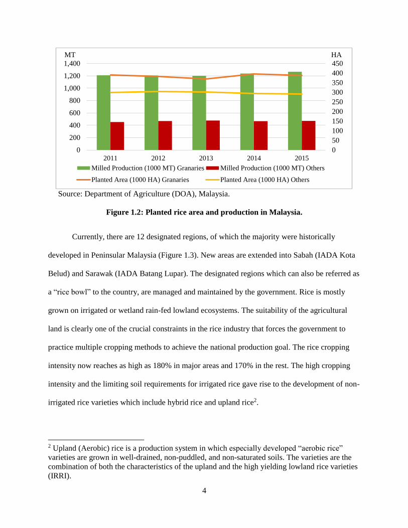
government. The designated rice production regions and their granaries play an important role in
the Malaysian rice industry, and the country is highly dependent on these areas to achieve self-
sufficiency goals. The granary regions produce 72.9% of domestic rice from 57% of the total
planted area in 2015/16 (Figure 1.2).
4
Source: Department of Agriculture (DOA), Malaysia.
Figure 1.2: Planted rice area and production in Malaysia.
Currently, there are 12 designated regions, of which the majority were historically
developed in Peninsular Malaysia (Figure 1.3). New areas are extended into Sabah (IADA Kota
Belud) and Sarawak (IADA Batang Lupar). The designated regions which can also be referred as
a “rice bowl” to the country, are managed and maintained by the government. Rice is mostly
grown on irrigated or wetland rain-fed lowland ecosystems. The suitability of the agricultural
land is clearly one of the crucial constraints in the rice industry that forces the government to
practice multiple cropping methods to achieve the national production goal. The rice cropping
intensity now reaches as high as 180% in major areas and 170% in the rest. The high cropping
intensity and the limiting soil requirements for irrigated rice gave rise to the development of non-
irrigated rice varieties which include hybrid rice and upland rice2.
2 Upland (Aerobic) rice is a production system in which especially developed “aerobic rice”
varieties are grown in well-drained, non-puddled, and non-saturated soils. The varieties are the
combination of both the characteristics of the upland and the high yielding lowland rice varieties
(IRRI).
0
50
100
150
200
250
300
350
400
450
0
200
400
600
800
1,000
1,200
1,400
2011 2012 2013 2014 2015
Milled Production (1000 MT) Granaries Milled Production (1000 MT) Others
Planted Area (1000 HA) Granaries Planted Area (1000 HA) Others
MT HA

5
Source: Ministry of Agriculture and Agro-based Industry (MOA), Malaysia.
Figure 1.3: Designated national rice producing areas in Peninsular Malaysia.
2. Significance of the Study
A twofold and long-standing rice policy goal in Malaysia is 1) to improve food security
and 2) to alleviate poverty among rice farmers. This largely dictates why the Malaysian
government constantly mandates rice self-sufficiency as a crucial national policy measure
(Ibrahim and Siwar, 2012; Tobias et al., 2012; Tey, 2010; Mohd Arshad and Abdel Hameed,
2010; Dano and Samonte, 2005). With limited agricultural land and high production costs, the
government intervenes heavily into the domestic rice industry through substantially providing
subsidies and price support programs to increase domestic production. These efforts are not only
to attain a high degree of self-sufficiency, but also to ensure economic welfare of both rice
farmers and consumers (Tey, 2010; Athukorala and Wai-Heng, 2007; Najim et al., 2007; Dano
and Samonte, 2005; Mustapha, 1998). Despite these supports, rice productivity has improved
6) KADA
7) IADA KEMASIN
SEMERAK
8) IADA KETARA
9) IADA PEKAN
10) IADA ROMPIN
1) MADA
4) IADA SEB.
PERAK
3) IADA
KERIAN SG
MANIK
2) IADA
PENANG
5) IADA BLS

6
slowly, and the nation has only produced between 65% to 70% of domestic requirements over
many years. Rice production grew slightly as the total production marginally increased by
0.87%, which comes from a yield improvement of 0.52% and an increase in area harvested of
0.32% in 2015/16 (Figure 1.4).
Source: Production, Supply, and Distribution (PS&D), USDA.
Figure 1.4: Rice production, area harvested, imports and yield in Malaysia.
Many studies have concluded that this marginal production growth has resulted from
inefficient policy strategies, which critically threatens overall food security3 (Siwar et al., 2014;
Abu, 2012; Vengedasalam et al., 2011; Mohamed Arshad et al., 2011; Mohamed Arshad and
Abdel Hameed, 2010; Tey, 2010; Athukorala and Wai-Heng, 2007; Dano and Samonte, 2005;
3 Food security refers to when all people at all times have physical and economic access to
sufficient food to meet their dietary needs for a productive and healthy life. Food security has
three dimensions: availability of sufficient quantities of food of appropriate quality, supplied
through domestic production or imports; access by households and individuals to adequate
resources to acquire appropriate foods for a nutritious diet; and utilization of food through
adequate diet, water, sanitation, and health care (Timmer, 2012).
0.00
0.50
1.00
1.50
2.00
2.50
3.00
0
200
400
600
800
1,000
1,200
1,400
1,600
1,800
2,000
Production (1000 MT) Area Harvested (1000 HA) Imports (1000 MT) Yield (MT/HA)
7
Mustapha, 1996). A simulation study by Md. Amin (1989) found that the fertilizer subsidy
programs provide a significant positive impact to improve rice yield, and thus increase the rice
production output, yet the input subsidy programs have failed to reduce cost of production due to
an upward trend in input market prices. With Malaysian farmers not likely to spend on additional
fertilizer if the subsidies are eliminated (Ramli et al., 2012), the removal of these subsidies might
negatively affect domestic rice production. It has also been argued that input subsidies are
capitalized into the cost of production, raising the value of fixed inputs such as land, and
paradoxically augmenting the cost of production. In addition, the price support policy was
discovered as an ineffective and a non-sustainable approach to increase rice production
(Mustapha, 1998; Baharumshah, 1991).
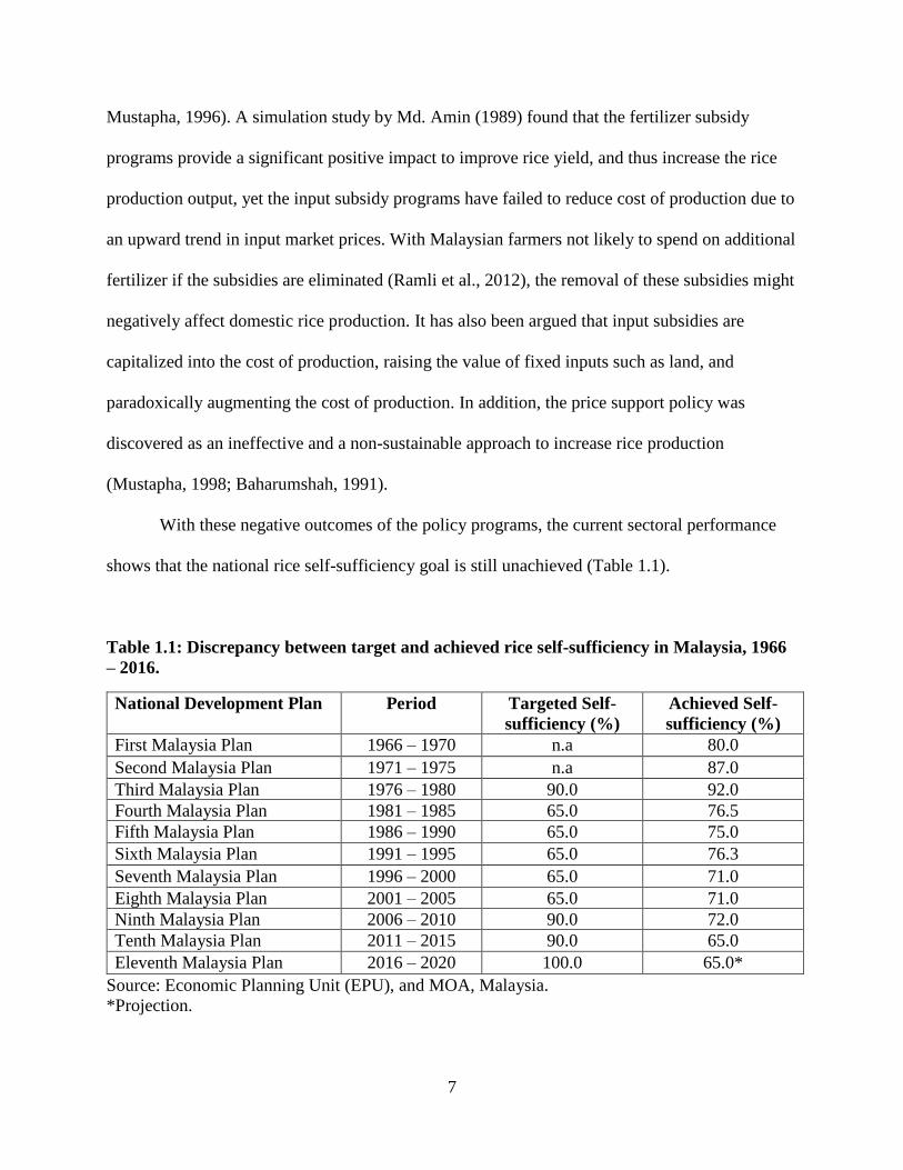
With these negative outcomes of the policy programs, the current sectoral performance
shows that the national rice self-sufficiency goal is still unachieved (Table 1.1).
Table 1.1: Discrepancy between target and achieved rice self-sufficiency in Malaysia, 1966
– 2016.
National Development Plan Period Targeted Self-
sufficiency (%)
Achieved Self-
sufficiency (%)
First Malaysia Plan 1966 – 1970 n.a 80.0
Second Malaysia Plan 1971 – 1975 n.a 87.0
Third Malaysia Plan 1976 – 1980 90.0 92.0
Fourth Malaysia Plan 1981 – 1985 65.0 76.5
Fifth Malaysia Plan 1986 – 1990 65.0 75.0
Sixth Malaysia Plan 1991 – 1995 65.0 76.3
Seventh Malaysia Plan 1996 – 2000 65.0 71.0
Eighth Malaysia Plan 2001 – 2005 65.0 71.0
Ninth Malaysia Plan 2006 – 2010 90.0 72.0
Tenth Malaysia Plan 2011 – 2015 90.0 65.0
Eleventh Malaysia Plan 2016 – 2020 100.0 65.0*
Source: Economic Planning Unit (EPU), and MOA, Malaysia.
*Projection.

8
The policy goal to attain rice self-sufficiency has failed, hence the stimulative policy measures
have not achieved the desired goals (Siwar et al., 2014; Abu, 2012; Vengedasalam et al., 2011;
Mohamed Arshad et al., 2011; Mohamed Arshad and Abdel Hameed, 2010; Tey, 2010;
Athukorala and Wai-Heng, 2007; Dano and Samonte, 2005; Mustapha, 1996). Despite the
government’s failed efforts, if the country attempts to achieve rice self-sufficiency, it would
come at a high cost both in terms of financial as well as societal costs (Mohamed Arshad et al.,
1983 and Abdullah et al, 2010). The interventionist instruments have also been debated in terms
of long-term sustainability which have resulted in a high budgetary burden to the government,
misallocation of resources, and demands for market liberalization. With the domestic
consumption continuing to grow in the future, rice remains significant for the entire Malaysian
population (Figure 1.5).
Source: International Rice Outlook (Wailes and Chavez, 2016).
Figure 1.5: Projections on domestic rice production and per capita use, 1982-2025.
0.0
20.0
40.0
60.0
80.0
100.0
120.0
0
500
1,000
1,500
2,000
2,500
3,000
3,500
19
82
19
84
19
86
19
88
19
90
19
92
19
94
19
96
19
98
20
00
20
02
20
04
20
06
20
08
20
10
20
12
20
14
20
16
20
18
20
20
20
22
20
24
Domestic consumption (1000 Mt) Per capita use (Kg)
9
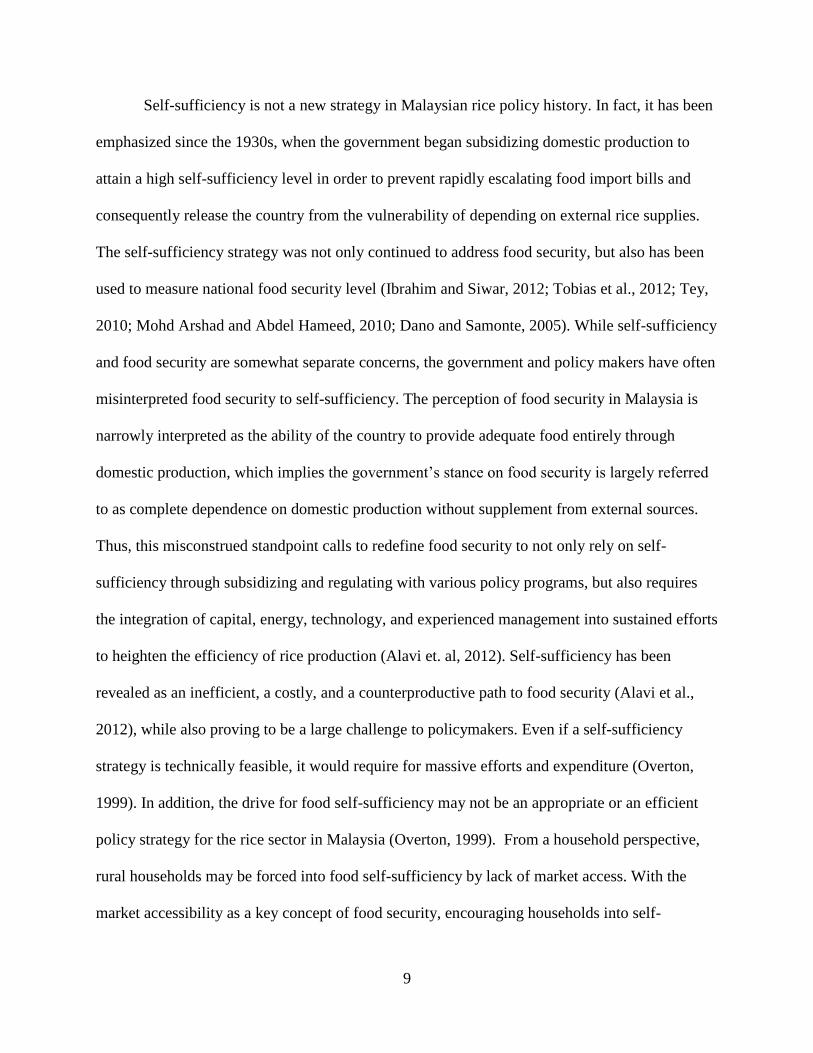
Self-sufficiency is not a new strategy in Malaysian rice policy history. In fact, it has been
emphasized since the 1930s, when the government began subsidizing domestic production to
attain a high self-sufficiency level in order to prevent rapidly escalating food import bills and
consequently release the country from the vulnerability of depending on external rice supplies.
The self-sufficiency strategy was not only continued to address food security, but also has been
used to measure national food security level (Ibrahim and Siwar, 2012; Tobias et al., 2012; Tey,
2010; Mohd Arshad and Abdel Hameed, 2010; Dano and Samonte, 2005). While self-sufficiency
and food security are somewhat separate concerns, the government and policy makers have often
misinterpreted food security to self-sufficiency. The perception of food security in Malaysia is
narrowly interpreted as the ability of the country to provide adequate food entirely through
domestic production, which implies the government’s stance on food security is largely referred
to as complete dependence on domestic production without supplement from external sources.
Thus, this misconstrued standpoint calls to redefine food security to not only rely on self-
sufficiency through subsidizing and regulating with various policy programs, but also requires
the integration of capital, energy, technology, and experienced management into sustained efforts
to heighten the efficiency of rice production (Alavi et. al, 2012). Self-sufficiency has been
revealed as an inefficient, a costly, and a counterproductive path to food security (Alavi et al.,
2012), while also proving to be a large challenge to policymakers. Even if a self-sufficiency
strategy is technically feasible, it would require for massive efforts and expenditure (Overton,
1999). In addition, the drive for food self-sufficiency may not be an appropriate or an efficient
policy strategy for the rice sector in Malaysia (Overton, 1999). From a household perspective,
rural households may be forced into food self-sufficiency by lack of market access. With the
market accessibility as a key concept of food security, encouraging households into self-
10
sufficiency is not a useful strategy to either achieve food security objectives or to reduce poverty
(Galero et. al., 2014). Because of this, self-sufficiency in rice is more likely to be more a political
strategy rather than a poverty-reducing rational (Timmer, 2010).
Having limited competitive rice production (Najim et al., 2007), Malaysia struggles to
achieve a rice self-sufficiency level, due to food security issues, financial burden, trade
agreements, and competition with industrial crops throughout the years. Malaysia embarked on
an ambitious goal to achieve self-sufficiency in the rice sector (Goldman, 1975) through heavy
government interventions. Tey (2010) suggested that the country certainly needs to reexamine
the current policy approach due to costly intervention, particularly on subsidy programs.
Furthermore, food self-sufficiency approach has been widely criticized as a misguided policy
decision and furthermore that it seeks to achieve food security that reflects political priorities
over economic efficiency (Clapp, 2017). The goal of self-sufficiency which means to food
security is a political goal while economically is distorted, costly, and inefficient, and thus the
Malaysian rice policy has become a political delusion (Dano and Samonte, 2005).
Future Malaysian rice production and supply are going to be more uncertain and may
result in more volatile prices (Ibrahim and Siwar, 2012; MOA, 2011). Even compared to the
widely accepted standard of sustainable agriculture4, the recent agricultural policies in Malaysia
are not supportive to sustainable agricultural practices (Murad et al., 2008). According to the
4 (1) Improved farm-level social and economic sustainability enhances farmer’s quality of life, (2)
increases farmers self-reliance, (3) sustains the viability/profitability of the farm, (4) improved
wider social and economic sustainability improves equity socially supportive and meets society's
needs for food and fiber, (5) increased yields and reduced losses while minimizing off-farm inputs,
(6) minimizing inputs from non-renewable sources, (6) maximizing use of (knowledge of) natural
biological processes and promoting local biodiversity/environmental quality (U.S Farm Bill, 1990;
Pretty, 1995; Ikerd, 1993; Hodge, 1993; Swedish Society for Nature Conservation, 1999).
11
International Rice Research Institute (IRRI), “the global rice market, which is relatively small
compared with that of other major food crops such as wheat, maize, and soybeans, is likely to
become even smaller if rice-consuming countries vigorously pursue self-sufficiency strategy. A
consequence of a smaller market is greater price volatility and, the smaller the market size is, the
more prices have to move in response to any supply and demand shock” (IRRI, 2016).
The typical policy responses by the net rice importing countries after the food crisis
generally involved the reduction of import duties, the building up of extra reserves, the reduction
of import restrictions, price controls through subsidies, and more importantly, the promotion of
self-sufficiency (Chandra and Lontoh, 2010). To a large extent, policy responses at the national
level have not only contributed to further global food price volatility (Slayton, 2009), but also
have undermined the food security situation in the region (Chandra and Lontoh, 2010). An ex-
post analysis of the 2008-food crisis found that government policies and panicky responses were
the key factors behind soaring rice prices (Alavi et al., 2012). There were also arguments that
the recent food crisis could have stemmed from a shift in policy towards heavy governmental
intervention to boost food production, control food prices, and provide more reliable access for
poor households, since the interventions involved significant costs (Timmer, 2010; Dawe, 2010).
The catastrophe of the crisis revealed the urgent need to reexamine and reform policies that
trigger not only the immediate catastrophe, but also the potential for recurrence. Unfortunately,
“The government interventions seem simply like attempts to recycle the past, harking back to
self-sufficiency5, while also reconsidering internal market emphasis during the 1960s and 1970s,
which fostered large productivity gains, improved crop yields, disease-resistant seeds, food
5 In the context of food security, the self-sufficiency ratio is indicated by the ratio of a country’s
own production relative to domestic consumption, i.e. the higher the ratio the greater the self-
sufficiency.

12
supply chain revolution, and so forth” (Alavi et al., 2012). Instead of needing to be developed for
the next phase of competitive capability, the rice sector has been pulled backwards, focusing on a
self-sufficiency strategy and pushing local rice production. While Malaysia often associates food
security with complete self-sufficiency as well as its dependency on government programs, food
security cannot easily be achieved through domestic production.
With the domestic production having been stagnant for many years, the elimination of
subsidies could potentially increase net welfare and government revenues (Vengedasalam et al.,
2011), but with changing the current import policies. Some research hypothesized that the price
support policy might have been justified on grounds of income distribution or the government’s
favor for political interests (Dano and Samonte, 2005; Baharumshah, 1991). In addition, the
authorization of BERNAS as a sole importer and distributor in the Malaysian rice sector would
not hide political reasons behind the sound of economic rationale (Dano and Samonte, 2005). A
“single-desk” import policy instrument can also threaten food security as the domestic support
price is staked above the world price under a monopsony market structure and the failure of the
government to control market price instability, resulting in severe inflation (Vengedasalam et al.,
2011). Thus, the policy decision of authorizing a sole importer has trade-distorting effects as the
government provides a privilege to be a monopsony rice buyer (Abu, 2012; Vengedesalam et al.,
2011).
Malaysia has been a net rice importer for many years and is expected to remain
dependent on rice imports in the future to support a domestic shortage supply. The baseline
projections using the Arkansas Global Rice Model (AGRM) indicate that Malaysia is likely to
import around 1.6 million tons in 2025 (Wailes and Chavez, 2016). Despite the call for a more

13
liberalized market by the World Trade Organization6 (WTO) since the 1960s, the importation of
rice reflects a trade-off of self-sufficiency for financial sustainability as imports are considered to
be cost saving (Mohamed Arshad et al., 2011; Tey, 2010; Mustapha, 1996). Malaysia’s
participation in free trade agreements (FTAs) suggests that opening to freer trade and elimination
of tariffs on rice is a key strategy going forward but also in conflict with the rice self-sufficiency
goal.
Alternatively, trade openness improves each dimension of food security, increasing food
availability through enabling products to flow from surplus to deficit regions (OECD, 2014). A
previous study projected that Malaysia would be able to sustain the maximum of 70% of self-
sufficiency in the long-term due to complying with trade agreements (Mohamed Arshad et. al,
2011). In theory, trade expands rice markets, and thus opens access to additional sources that
could be a remedial approach to domestic production scarcity, so that rice supply and demand
would be met. In fact, trade balances the deficits of net food importers with the surpluses of rice
exporting countries. In the absence of trade, food prices would be higher in net importing
countries in order to bring national supply and demand into equilibrium, potentially worsening
the food security status quo in those countries. In addition, rice imports may help lower food
prices for poor, low-income, and undernourished groups, which is crucial in times of disruptions
to and uncertainty of domestic production, from climate change, crop diseases, and so forth.
According to the World Bank, the liberalization exercise contributes to a reduction in poverty
incidence among farm households without exacerbating income inequality and thus generates
gains to the poor (Ganesh, 2005). Durand-Morat and Wailes (2011) postulated that Malaysia has
6 The World Trade Organization (WTO) is the only global international organization dealing
with the rules of trade between nations, primarily the WTO agreements, negotiated and signed by
the bulk of the world’s trading nations and ratified in their parliaments. The goal is to help
producers of goods and services, exporters, and importers conduct their business.

14
the potential to be a food secured nation resulting from rice trade liberalization through a
significant decrease in consumer prices. Regional trade agreements are hypothesized to receive
positive responses from participants. “Since the issuance of the ASEAN Integrated Food
Security framework in 2008 and the further successful adoption of the ASEAN Trade in Goods
and Agreement7 (ATIGA) in 2009, rice deficit countries within the region would prefer to hang
tenaciously on their long-held goal of rice self-sufficiency” (Alavi et al., 2012). The Trans-
Pacific Partnership8 (TPP) agreement also seeks to open trade initiatives among the members,
particularly major rice exporters – Vietnam and Australia – thus contributing to food security
(Malaysia International Trade Industry, 2015). Given that the self-sufficiency strategy in
Malaysia’s rice sector is misconstrued towards food security as well as rice farmers’ and
consumers’ welfare, it is crucial to evaluate and analyze the national rice development policy
comprehensively.
3. Purpose of Research
The general objective of this study is to examine deep-rooted national rice policy
strategies in Malaysia. This encompasses the evaluation of a long-held self-sufficiency policy
strategy to address food security and poverty concerns in light of the country’s regional and
bilateral trade participations. The specific objectives below will be achieved in comprehensive
studies in Chapter II, III, and IV:
7 ASEAN Trade in Goods Agreement (ATIGA) aims to achieve free flow of goods in the region
resulting to less trade barriers and deeper economic linkages among members, lower business
costs, increased trade, and a larger market and economies of scale for businesses (ASEAN,
2017). 8 The Trans-Pacific Partnership (TPP) agreement is a trade agreement between Australia, Brunei,
Canada, Chile, Japan, Malaysia, Mexico, New Zealand, Peru, Singapore, Vietnam, and the
United States (until January 23, 2017).

15
1) To measure the profitability, competitiveness, and the efficiency at production level of rice
industry in Malaysia using a Policy Analysis Matrix (PAM) framework.
2) To estimate the impact of rice self-sufficiency and international trade policies in Malaysia at
the national level using a partial, spatial equilibrium model.
3) To measure the impacts of international trade policy on rice production and consumption,
poverty, and farmers’ welfare at the household level on individual rice farmers in Malaysia
using a Farm-Household model.
This research will address these overarching questions:
1) Should Malaysia maintain the current policy to pursue self-sufficiency in rice? (in both
political and economic perspectives)
2) What are the consequences and welfare impacts of pursuing self-sufficiency in rice to
farmers, consumers, and the government?
3) If Malaysia anticipates eliminating rice imports, how could the country achieve self-
sufficiency in rice with respect to policy requirements?
4) What are the impacts of allowing free trade in rice on farmers, consumers, and the
government?
5) How does the free trade policy affect individual rice farmers with respect to rice production
and consumption, poverty, and welfare?
These policy evaluations and analysis would help to identify holistic impacts of the self-
sufficiency and international trade policies on rice farmers, consumers, and the government at
both the macro and micro levels.

16
4. Research Approach
This dissertation research evaluates rice policy interventionist strategies, and the impacts
of self-sufficiency, international free trade, and food security at the national and farm-household
levels to address the rice policy concerns in Malaysia. A comprehensive evaluation will be
conducted covering the rice policy from the production level to the market, through conducting
different research analyses and using different quantitative methods to measure the impact of rice
policies holistically on farmers, consumers, and the government. This study begins with
evaluating the competitiveness and efficiency in rice production policy using the Policy Analysis
Matrix approach. The impact of self-sufficiency and international trade policies is presented in
Chapter III using the RICEFLOW model to simulate alternative outcomes. Chapter IV analyzes
the impact of international trade policy on rice farmers using the Farm-Household model. The
results of the study will reveal the (in)efficiency of the food security policy.
4.1 Competitiveness and Efficiency in Rice Production
While limited studies attempt to measure competitiveness and efficiency of the rice
industry in Malaysia, a few studies concluded that the industry has no clear comparative
advantage. The evaluation at the production level visualizes the production performance given
current technologies and policies. Using the Policy Analysis Matrix (PAM), originated by
Monke and Pearson (1989), this study quantitatively measures the impact of the interventionist
policies on profitability and the efficiency of resource used in the rice production system, and
thus the competitiveness and the comparative advantage of the rice industry can be analyzed.
PAM is a recognized approach and has been widely applied in the agricultural sector to
implement an analytical process and to act as an empirical method for measuring the effects of

17
policy on the rice sector. PAM provides a helpful framework to understand the effects of policy
and serves as a useful tool to measure the magnitudes of policy transfers. Therefore, PAM can
address and investigate crucial policy concerns, dealing with the competitiveness of production
systems, which are associated with farm incomes, the efficient allocation of resources in
agriculture and the comparative advantage, and the effects of policy and market failures with the
allocation of investment to the agricultural sector (i.e. policy transfers).
4.2 Evaluations and Analysis of Self-sufficiency and International Trade
With the production status quo having been estimated in the PAM analysis, this study
estimates deeper policy consequences of self-sufficiency and international trade policies on the
rice sector at the macro level. The simulated estimations focus on the producer prices, consumer
prices, domestic production, and rice imports under the self-sufficiency and free trade scenarios.
From the self-sufficiency scenario, we then measure the subsidy, production factor, and
technological efficiency requirements. From these measures, the government revenue or losses
can also be identified and estimated. As the government recently decided to pursue self-
sufficiency through removing bilateral rice trade, the impact of the self-sufficiency strategy has
become extremely important to be determined which could provide a useful perspective for the
government and policymakers in rice policy decisions. This study utilizes a partial, spatial
equilibrium model, developed by Durand-Morat and Wailes (2010) that is based upon a spatial
price equilibrium model specified by Takayama and Judge (1964). The model is identified as a
spatial partial equilibrium of the global rice economy which simulates the behavior of the entire
rice supply chain, from input markets to final consumption in multiple regions.

18
4.3 Evaluations and Analysis of International Trade on Farm-Household
The price estimations from the RICEFLOW simulation analysis are then applied at the
micro level to measure the impact of rice policy to individual rice farmers at the household level,
since farmers play an important role in achieving the rice policy goal. In addition, rice policy has
aimed to improve livelihood and welfare, and to alleviate poverty among rice farmers for
decades, thus determining the impact of rice policy at the farm household level is crucial. This
study measures the impact of free trade policy on rice farmers. Although Malaysia actively
participates in free trade agreements at both bilateral and regional levels, rice has been excluded
from the agreements as it is identified and classified as a sensitive commodity. The government
stance has been to favor rice farmers on an individual level without consideration being given
how the policy affects the economy as a whole. On a purely theoretical level, free trade does hurt
local rice farmers, yet, the magnitude of the impact requires a comprehensive study so that the
effects can be quantitatively measured. This study develops a farm-household model for the
individual rice farmers in Malaysia to measure the effects of the free trade on rice farmers with
respect to poverty and welfare.
The three studies are organized to begin with: 1) the evaluation at the production level
through evaluating the protectionist rice production policy in Chapter II, 2) the impact of self-
sufficiency and international trade policies at the national level in Chapter III, and 3) the impact
of international trade policies at the farm household level in Chapter IV. The policy implications
from these comprehensive studies are discussed in Chapter V as the concluding remarks.

19
References
Abdullah, A. M., Mohamed Arshad, F., Radam, A., Ismail, M. M., Yacob, M.R., Harron, M.,
Mohamed, Z. A., Abd Latif, I., and Alias, E. F. 2010. Kajian Impak Skim Subsidi Baja
Padi Kerajaan Persekutuan (SSBPKP) dan Skim Subsidi Harga Padi (SSHP). Research
Report, Selangor: Universiti Putra Malaysia: Institut Kajian Dasar Pertanian dan
Makanan.
Abu, N. 2012. Paddy and Rice Policy Transformational: A Historical Policy Analysis. Research
Report, Japan: Higher Degree Committee Of Ritsumeikan Asia Pacific University.
Alavi, H. R., Htenas, A., Kopicki, R., Shepherd, A. W., and Clarete, R. 2012. Trusting Trade and
the Private Sector for Food Security in Southeast Asia. World Bank.
Athukorala, P., and Wai-Heng, L. 2007. Distortions to Agricultural Incentives in Malaysia.
Agricultural Distortion Working Paper, The World Bank Development Research Group.
Baharumshah, A. Z. 1991. "A Model for the Rice and Wheat Economy in Malaysia: An
Empirical Assessment of Alternative Specifications." PERTANIKA, 383 – 391.
Chandra, A. C., and Lontoh, L. A. 2010. Regional Food Security and Trade Policy in Southeast
Asia:The Role of ASEAN. Regional Report, International Institute for Sustainable
Development.
Chen, C.H., C.C. Mai, C.C., and Yu, C, H. 2006. The effect of export tax rebates on export
performance: theory and evidence from China.
Cramer, G., Wailes, E., and Shui, S. (1993). Impacts of liberalizing trade in the world rice
market, American Journal of Agricultural Economics 75(1), 219–226.
Dano, E. C., and Samonte, E.D. 2005. "Public Sector Intervention In The Rice Industry In
Malaysia." Southeast Asia Regional Initiatives for Community Empowerment
(SEARICE). Accessed March 7, 2017. http://www.zef.de.
Dawe, D. and Slayton, T. 2010. "The World Rice Market Crisis Of 2007-08." Food and
Agriculture Organization (FAO) and Earthscan.

20
Dawe, D. 2010. The Rice Crisis. Food and Agriculture Organization.
Department of Agriculture, Malaysia (DOA). 2010. Subsidy and Agricultural Incentives for
Farmers. www.pmr.penerangan.gov.my.
Durand-Morat, A., and Wailes, E. J. 2011 . "Rice Trade Policies and Their Implications for Food
Security." Agricultural & Applied Economics Association’s AAEA & NAREA Joint
Annual Meeting. Pittsburgh, Pennsylvania.
Durand-Morat, A and Wailes, E. (2010). A Multi-Region, Multi-Project, Spatial Partial
Equilibrium Model of the World Rice Economy.
Eddie C. Chavez, E.C., Wailes, E.J., and Durand-Morat, A. 2014. "Trade and Price Impacts of
Thailand Paddy Pledging Program on The Global Rice Market ." Southern Agricultural
Economics Association Annual Meeting. Dallas, Texas.
Ganesh, S. 2005. The Impact of Trade Liberalization on Household Welfare in Vietnam. Policy
Research Working Paper, Washington, DC: The World Bank.
Fan, S., E. J. Wailes, E.J., and G. L. Cramer, G.L. 1995. Household Demand in Rural China: A
Two-Stage LES-AIDS Model. American Journal of Agricultural Economics. 77:54-62.
Food and Agriculture Organization (FAO). 2014. FAO Rice Market Monitor. Accessed March 7,
2017. www.fao.org.
Food and Agriculture Organization (FAO). 2008. Soaring Food Prices: Facts, Perspectives,
Impacts, and Actions Required. Research Report, Rome, Italy.
Food and Agriculture Organization. 2010. The Global Food Crisis.
Galero, S., So, S.,and Tiongco, M. 2014. Food Security versus Rice Self-Sufficiency: Policy
Lessons from the Philippines . Research Report, De La Salle University, Manila,
Philippines, DLSU Research Congress.

21
Goldman, R, H. 1975. "Staple Food Self-Sufficiency and the Distributive Impact of Malaysian
Rice Policy." Food Research Institute Studies.
Headey, D. and Fan, S. 2010. Reflections on the Global Food Crisis How Did It Happen? How
Has It Hurt? And How Can We Prevent the Next One? Research Monograph,
Washington: International Food Policy Research Institute.
Hodge, I., 1993. Sustainability: Putting Principles into Practice. Paper presented to Rural
Economy and Society Study Group at Royal Holloway College, December 1993.
Ibrahim, A. Z. and Siwar, C. 2012. "Kawasan Pengairan Muda: Merentasi Masa Menyangga
Keselamatan Makanan Negara." Jurnal Pengurusan Awam 69 – 90.
Ikerd, J., 1993. Two Related but distinctly different concepts: Organic farming and sustainable
agriculture. Small Farm Today, 10: 30-31.
International Rice Research Institute, IRRI. 2016. International Rice Market and Trade. March
7. Accessed March 7, 2016. http://ricepedia.org.
International Rice Research Institute, IRRI. 2013. Trend in Global Rice Consumption. March 7.
Accessed Oct. 27, 2017. https://www.scribd.com/document/
Magno, C.R., and Yanagida, F.J. 2000. Effect of Trade Liberalization in the Short-Grain
Japonica Rice Market: A Spatial Temporal Equilibrium Analysis. Philippine Journal of
Development, No.49, Vol. XXVII.
McCulloch, N. and Timmer, P. 2008. Rice Policy in Indonesia: A Special Issue. Bulletin of
Indonesian Economic Studies, http://econpapers.repec.org, 34–44.
Md. Amin, M. A. 1989. "Subsidi dan Kesannya ke atas Petani Padi." Jurnal Ekonomi Malaysia
(19): 17-30.
Ministry of Agriculture and Agro-based Industry (MOA). 2011. National Agro-Food Policy
(2011 - 2020). National Development Policy, Putrajaya: MOA.

22
Ministry of Finance, Malaysia. 2014. National Audit Report. Putrajaya.
Ministry of International Trade and Industry (MITI). 2015. TPPA-Perjanjian Perkongsian
Trans-Pasifik: Jawapan Kepada Kebimbangan, Salah Faham, dan Tuduhan. . Ministry
Report, Kuala Lumpur, Malaysia: Ministry of International Trade and Industry (MITI).
Mohamed Arshad, F., Alias, E. F., Mohd Noh, K., Tasrif, M. 2011. "Food Security: Self-
Sufficient of Rice in Malaysia." Int. J. Manage. Stud. 18 (2): 83-100.
Mohd Arshad, F., and Abdel Hameed, A. A. 2010. "Global Food Prices: Implications for Food
Security in Malaysia." Journal of the Consumer Research and Resources Centre (CRRC
Consumer Review ) 21 – 37.
Mohd. Arshad, F., Mohayidin, M.G., Ayub, A.M., and Husin, M. 1983. The Impact of Paddy
Subsidy Schemes on Malaysian Farmers. Consultancy Report, Kuala Lumpur: Ministry
of Public Enterprise, 421.
Monke, E., and Pearson, S. 1989. The Policy Analysis Matrix for Agricultural Development.
Cornell University Press, Ithaca and London.
Murad, M. W., Nik Mustapha, N. H., Siwar, C. 2008. Review of Malaysian Agricultural Policies
with Regards to Sustainability. Policy Review, Department of Economics, Faculty of
Management and Economics, Terengganu, Malaysia: University of Malaysia
Terengganu.
Mustapha, N. H. 1998. "Welfare Gains and Losses under the Malaysian Rice Pricing Policy and
their Relationships to the Self-Sufficiency Level." Jurnal Ekonomi Malaysia 32: 75 – 96.
Mustapha, N.H. 1996. "Sustainable Development of Malaysian Rice Industry in the Context of
Asian Countries: An Assessment." Jurnal Ekonomi Malaysia 67 – 86.
Najim, M.M., Lee, T.S., Haque, M.A., and Esham, M. 2007. "Sustainability of Rice Production:
A Malaysian Perspective." The Journal of Agricultural Science 3.
Nee, A.Y.H. 2008. "Supply Chain Model For Rice In Malaysia – Basics And Challenges." ECER
Regional Conference. Kota Bharu, Kelantan.

23
New Straits Times. 2014. Malaysia Hopes to End Rice Imports By 2020. April 4.
OECD - Organization for Economic Co-operation and Development. 2014. "Trade Dimensions
of Food Security." Working Party on Agricultural Policies and Markets.
Overton, J. 1999. "Integration or Self-Sufficiency? Peninsular Malaysia and the Rice Trade in
Southeast Asia." Singapore Journal of Tropical Geography (Wiley Online Library) 20
(2): 169-180.
Pandey, S., Sulser. T., Rosegrant, M., Bhandari, H. 2010. "Rice Price Crisis: Causes, Impacts,
and Solutions." Asian Journal of Agriculture and Development 7 (2): 1-15.
Pretty, J., 1995. Regenerating Agriculture: Policies and Practice for Sustainability and Self-
Reliance. Earthscan Publications, London.
Rajamoorthy, Y., Abdul Rahim, K., Munusamy, S. 2015. "Rice Industry in Malaysia:
Challenges, Policies and Implications." Procedia Economics and Finance (31): 861-867.
Ramli, N., Shamsudin, M., Mohamed, Z., and Radam, A. 2012. "The Impact of Fertilizer
Subsidy on Malaysia Paddy/Rice Industry Using a System Dynamics Approach."
International Journal of Social Science and Humanity 2 (3).
Siwar, C., Idris, N. D. M., Yasar, M., and Morshed, G. 2014. "Issues and Challenges Facing Rice
Production and Food Security in the Granary Areas in the East Coast Economic Region
(ECER), Malaysia."
Swedish Society for Nature Conservation, 1999. Policy for Sustainable Agriculture. Birger
Gustafsson AB, Stockholm, Sweden.
Takayama, T. and Judge, G.G. 1971. Spatial and Temporal Price and Allocation Models.
Amsterdam: North-Holland Publishing Company.
Tey, Y. S. 2010. "Review Article Malaysia’s Strategic Food Security Approach." International
Food Research 17: 501-507.

24
The International Rice Research Institute (IRRI). 2013. Rice Basics. IRRI.
The Sun Daily. (2016). Malaysia hopes to halt import of food products by 2050.
Timmer, P. C. 2010. "Behavioral Dimensions of Food Security." Proceedings of National
Academy of Sciences of United States of America.
Timmer, P.C. 2010. "Preventing Food Crises Using A Food Policy Approach." The Journal of
Nutrition (American Society for Nutrition).
Tobias, A., Molina, I., Valera, H. G., Abdul Mottaleb, K., and Mohanty, S. 2012. "Handbook on
Rice Policy for Asia." econpapers.repec.org. Accessed March 7, 2017.
http://econpapers.repec.org.
United States Farm Bill. 1990. Food, Agriculture, Conservation and Trade Act of 1990. Public
Law 101-624, Title XVI, Subtitle A, Section 1603. Government Printing Office,
Washington DC., United States of America.
Vengedasalam, D., Harris, M., and MacAulay, G. 2011. "Malaysian Rice Trade and Government
Interventions." 55th Annual Conference of Australian Agricultural and Resource
Economic Society.
Wailes, E. and E. Chavez. 2016. "International Rice Outlook: Baseline Projections 2015-2025."
Staff Paper.
World Bank. 2011. Responding To Global Food Price Volatility and Its Impact On Food
Security. Development Comittee Report, The World Bank.
World Bank. 2012. Severe Droughts Drive Food Prices Higher, Threatening the Poor. Press
Release, Washington: The World Bank Group.

25
Appendix Table 1.1: Current rice subsidy and policy programs in Malaysia.
Policy Program Description
Agricultural
Input
Fertilizer subsidy of Federal
Government Scheme
4 bags/ ha @ 20 kg/bag of Urea
12 bags/ha @ 20 kg/bag of Compound (NPK)
Paddy production incentive of
additional fertilizer
5 bags/ha @ 20 kg/bag of Organic, or
6 bottle/ha @ 1 liter/bottle of Foliar
Rice production incentive for
National Food Security Policy
Additional NPK: 6 bags/ha/season; 25 kg/bag
Pesticides: RM200/ha/season
Chemical: 3 Mt/ha (Once in 3 years)
Paddy seed incentive RM 1.03/kg (Paddy seed producers receive the
value for supplying rice seeds)
Labor Paddy production incentive
(plowing)
RM 100/ha (Farmers receive the value for
wages in plowing)
Production
Output
Paddy price subsidy RM 1,200/Mt (Farmers are paid at a producer
price support)
Paddy production subsidy
RM300/Mt (Farmers receives the value from
output production)
Yield increase incentive RM 650/Mt (Farmers receive the value for
yield increase)
Consumption Rice subsidy
Rice voucher to low income group for ST15%
International
Trade
ASEAN Trade in Goods
Agreement (ATIGA)
20% ad valorem tariff of rice imports from
most favored nations (MFN)
Agreement on Agriculture9 (AoA)
of the World Trade Organization
(WTO)
40% ad valorem tariff of rice import
Source: Ministry of Agriculture and Agro-based Industry, Malaysia; Ministry of International
Trade and Industry (MITI).
9 The Agreement on Agriculture (AoA) was negotiated during the Uruguay Round of the General
Agreement on Tariffs and Trade, and entered into force with the establishment of the WTO on
January 1, 1995.

26
Chapter II
Measuring the Competitiveness and Efficiency of Rice Sector in Malaysia Using Policy
Analysis Matrix
Abstract
Despite having exerted distorting effects on not only rice markets, but also production
input and factors markets, protectionist policies remain the most favored government’s policy
strategy in Malaysian rice industry. A wide range of policy programs have been mandated, which
mainly embrace input and output subsidies, and producer support price in line with the self-
sufficiency goal. Despite its small contribution to the national income, rice receives special
attention and has been given a priority in series of the national development policies and
resources due to a crucial and sensitive political issue to maintain rice farmers’ livelihoods and
welfare. Using the policy analysis matrix approach, this study measures the extent to which rice
policies have distorted domestic markets and the impacts of the interventionist policies on rice
production in Malaysia. The results reveal that without domestic supports, rice production is
significantly unprofitable. Despite having been protected by the government, the rice production
system is not competitive, and the protectionist strategy leads to policy distortions. Relative to
rice imports, domestic rice has no comparative advantage since the imported rice indicates much
lower at the comparable world price. Therefore, the government’s interventionist policy
instruments significantly have failed to drive competitiveness in the rice sector. In fact, policy
distortions would induce unnecessary efficiency losses to realize the national self-sufficiency
goal. Hence, the government policies should focus on the economic development at the macro
level instead of stimulating policies to highly subsidize the rice economy. This study provides
key measures of the effects of rice policies on the Malaysian rice production system that could be
a guideline for policy decisions.
27
1. Introduction
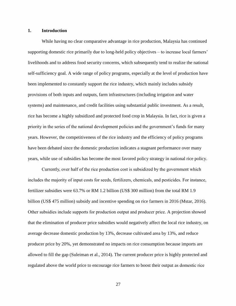
While having no clear comparative advantage in rice production, Malaysia has continued
supporting domestic rice primarily due to long-held policy objectives – to increase local farmers’
livelihoods and to address food security concerns, which subsequently tend to realize the national
self-sufficiency goal. A wide range of policy programs, especially at the level of production have
been implemented to constantly support the rice industry, which mainly includes subsidy
provisions of both inputs and outputs, farm infrastructures (including irrigation and water
systems) and maintenance, and credit facilities using substantial public investment. As a result,
rice has become a highly subsidized and protected food crop in Malaysia. In fact, rice is given a
priority in the series of the national development policies and the government’s funds for many
years. However, the competitiveness of the rice industry and the efficiency of policy programs
have been debated since the domestic production indicates a stagnant performance over many
years, while use of subsidies has become the most favored policy strategy in national rice policy.
Currently, over half of the rice production cost is subsidized by the government which
includes the majority of input costs for seeds, fertilizers, chemicals, and pesticides. For instance,
fertilizer subsidies were 63.7% or RM 1.2 billion (US$ 300 million) from the total RM 1.9
billion (US$ 475 million) subsidy and incentive spending on rice farmers in 2016 (Mstar, 2016).
Other subsidies include supports for production output and producer price. A projection showed
that the elimination of producer price subsidies would negatively affect the local rice industry, on
average decrease domestic production by 13%, decrease cultivated area by 13%, and reduce
producer price by 20%, yet demonstrated no impacts on rice consumption because imports are
allowed to fill the gap (Suleiman et al., 2014). The current producer price is highly protected and
regulated above the world price to encourage rice farmers to boost their output as domestic rice

28
sector has not been able to compete in an open market (Mohamed Arshad et al., 2007). The
government also regards the subsidy programs as a crucial and sensitive political issue to
maintain support of the rural sector since poverty is relatively high among rice farmers who
mostly are Malays (Mohamad Arshad and Mohayidin, 1990).
In spite of government efforts to achieve a high degree of rice self-sufficiency, over the
past several decades, rice production can only satisfy between 65% and 70% of domestic
consumption each year. Several studies have found that the unfavorable outcomes stemmed from
inefficient policy strategies due to the emphasis on self-sufficiency. Although studies also
suggested significant positive effects of fertilizer subsidies on rice production, a substantial
amount of subsidies would be reflected in costly use of tax payers’ dollars and higher
consumers’ prices, yet since domestic production has been dormant for years, elimination of
subsidies could potentially increase the economic net welfare and government revenues
(Vengedasalam et al., 2011). Malaysia has practiced a price support policy in the rice sector
since 1949, perhaps due to colonial roots, to purportedly guarantee the welfare of both rice
farmers and consumers, claiming that this offers a fair price to both sides. The domestic producer
price has recently increased to RM 1,200 (US$ 300) per metric ton paddy basis while the current
world market rice price was US$ 280 per metric ton (United Nation, 2016). Despite having
shown positive impacts to self-sufficiency, food security, and production sustainability, the
producer price subsidy led to losses for the government (Mustapha, 1998). In addition, the Public
Accounts Committee of Malaysia (PAC) reported significant difficulties administering the most
recent subsidy, which were misappropriated during the reimbursement process to the appointed
private vendors due to the management and supervisory deficiencies that resulted in a
discrepancy in government accounts (Berita Harian, 2016).
29
Given those shortcomings, why does the government continue subsidizing rice farmers?
Although the government is often motivated to provide production subsidies for farmers’
livelihoods and welfare, it is possible that subsidies, which are supposed to be an economic
effort, have been inappropriately abused and misused by interest groups and those seeking
patronage, thus turning them into a political tool. It has been argued that, using taxpayers’
dollars, the subsidies acted as an ‘exchange’ for political votes, hence rice in Malaysia becomes a
political commodity. Often, monolithic political interests intrude on policy decisions, causing the
government to constantly intervene in the rice domestic rice industry. This study evaluates and
analyzes the impact of government protectionist policy on the rice sector and industry in
Malaysia. The specific objectives are: 1) to measure the profitability of rice production at a
private and social level of production costs; 2) to measure the competitiveness and efficiency that
are reflected in policy transfer; and 3) to provide useful economic perspectives to the government
and policymakers.
2. Theoretical Framework of Interventionist Policies
Government intervention, mainly subsidy and trade barriers have affected input and
output prices that causes domestic prices to differ from international market prices. The
interventionist policies drive a wedge between the world and the domestic price, restrict imports,
and thus raise the domestic price above the world price. Either of those policies are intended to
support producers, a subsidy and trade barrier transfer costs to consumers and the government
resulting in welfare losses. The price changes would create policy distortions in some ways: 1)
the quantities of the commodity that are produced, consumed, and traded (imported or exported),

30
2) the income transfers to/from producers, consumers, and the government budget, and 3) the
efficiency losses in production and consumption.
The graphical description of input subsidy policy implication is shown in Figure 2.610.
This figure indicates that the market price for rice (P1) shifts down from the equilibrium price
(Po), Po to P1, which implies consumers pay a lower price when production inputs are being
subsidized, thus encouraging farmers to produce more outputs. Both farmers and consumers are
better off from the input subsidy as both producer and consumer surpluses increase. Change in
producer surplus is a gain of area a and b. Change in consumer surplus is a gain of c, d, and e.
The total cost of subsidy is area a, b, c, d, e, and f, while f indicates the deadweight loss. The
subsidy leads to a net economic loss to the country and an income transfer from taxpayers to
consumers and producers. The government loses from the input subsidy policy, paying the input
subsidy costs.
Figure 2.6: Welfare effects of domestic production subsidies.
10 The graph does not follow the exact scale and coordinate, and therefore the affected areas do
not represent the actual amount and quantity.
Quantity
P1
Po
D (Demand)
Q1
Qo
S1 (Supply with subsidies)
d
a b
c f
e
P1 + Subsidy
Price So (Supply)

31
A producer price support policy raises the producer price (P1) above the original market
equilibrium price. This figure implies that consumers pay for the price support. The consumers
surplus loss is the area below the demand curve and between P and P1 (a + b). The producer
surplus gain is the area above the supply curve between the P and P1 (a, b and c). The surplus
production Q2 – Q1 has a market value where Q2 intersects the demand curve. However, if the
government pays for the price support then the market price will fall where the Q intersects the
demand curve benefitting consumers. The government loses from the guaranteed producer price
policy (Figure 2.7).
Figure 2.7: Welfare effects of producer price support policy.
Quantity
Guaranteed price
Demand
Q1 Q2
P1
Q
Price
Supply
P
a b c
32
3. Data and Method
3.1 Data Integration
This study utilizes secondary data from the government reports and databases from
various institutions which include production budgets for rice and import prices. The production
budgets were obtained from the annual reports by the Malaysian Department of Agriculture
(DOA) and Farmers’ Organization Authority (LPP) in production years 2014 and 2015. These
production budgets were obtained for the major rice producing regions in Peninsular Malaysia,
which are the largest rice subsidy recipients and are highly regulated by the government.
Therefore, the costs and revenues data from these regions are considered the most accurate
sources to be analyzed and thus represent the observed data for the effect of policy transfer
analysis in the Malaysian rice production system. The CIF (cost, insurance, and freight) and the
FOB (free on board) prices are obtained from the Malaysian Department of Statistics (DOSM)
and the United Nation Comtrade database for 2014/15 marketing year. These prices are used to
estimate the world comparable price at social level. The transportation, handling, and distribution
costs of rice imports are obtained from BERNAS, the solely rice importer. With these data, both
private and social valuations can be estimated.
3.2 Policy Analysis Matrix
To estimate private profits, social profits, and the effects of divergences, the principal
analysis of this study employs the policy analysis matrix (PAM) approach which can also
measure the competitiveness and the efficiency of rice production in Malaysia. PAM which was
developed by Monke and Pearson (1989), is widely used and recognized as a useful method to
analyze the impact of government policy on the profitability of agricultural systems and on the
efficiency of resource use (see example: Yao, 1997; Ekasingh et al., 2000; Elbadawi et al, 2013;

33
Ude et al, 2013; Kanaka and Chinnadurai, 2013; Akramov and Malek, 2012; Basavaraj et al.,
2013; Dibrova and Chan-khi, 2013; Mamza et al., 2014; Mantau et al., 2014; Pearson et al.,
2003; Rae and Kasryno, 1993; Martinez et al., 2008; Olowa, 2014; Zheng et al., 2013; Khai and
Yabe, 2013). PAM can also identify the effects of efficiency of interventionist policy which
incurs any efficiency losses associated with a distorting policy. PAM is a quantitative economic
analysis which utilizes a budget-based method, and thus allows one to evaluate and analyze
development projects of public investments which stimulate the government policy programs in
the agricultural sector (Monke and Pearson 1989; Gotsch et al., 2003). The production budgets
are initially valued to further measure private and social profitability of a production system.
Private budgets are based on current market prices paid and received by farmers, while social
budgets are based on social prices that account for government policy programs that affect the
market prices due to subsidies or taxes. “PAM approach to agricultural policy analysis can
provide decision-makers and analysts with both a helpful conceptual construct for understanding
the effects of policy and a useful technique for measuring the magnitudes of policy transfers”
(Monke and Pearson, 1989).
PAM has two major parameter identities: 1) profitability and 2) divergence, which are
measured across the matrix. Profits are defined as the difference between total (per unit) sales
revenues and costs of production. They are measured at two different prices – private and social
prices. The revenues represent the receipts that producers received from a production system,
while production costs are the expenditure of the tradable intermediate inputs (i.e. fertilizer,
pesticides, seed, transportation, etc.) and factors of production (i.e. labor and land). The
divergence is estimated as the difference in revenues and costs between private and social prices,
which then implies the effects of distorting policies and market failures. The analysis which

34
utilizes an accounting matrix procedure also measures the extent of transfers that affected by the
set of implemented policies and the inherent economic efficiency of a production system. Table
2.2 shows the structure of PAM and how parameters are measured.
Table 2.2: The structure of policy analysis matrix.
Costs Profits
Revenues Tradable Inputs Domestic Factors
Private profit
∑ 𝑝𝑛𝑡𝐷 𝑞𝑛𝑡
𝐷
∑ 𝑝𝑖𝑡
𝐷 𝑞𝑖𝐷
𝑖
∑ 𝑤𝑗𝑡𝐷 𝑙𝑗
𝐷𝑗
D=A-B-C
A B C
Social profit
∑ 𝑝𝑛𝑡𝑆 𝑞𝑛𝑡
𝑆 ∑ 𝑝𝑖𝑡
𝑆 𝑞𝑖𝑆
𝑖
∑ 𝑤𝑗𝑡
𝑆 𝑙𝑗𝑆
𝑗
H=E-F-G
E F G
Effects of
Divergences
∑ 𝑝𝑛𝑡𝐷 𝑞𝑛𝑡
𝐷 -
∑ 𝑝𝑛𝑡𝑆 𝑞𝑛𝑡
𝑆
∑ 𝑝𝑖𝑡
𝐷 𝑞𝑖𝐷
𝑖 - ∑ 𝑝𝑖𝑡
𝑆 𝑞𝑖𝑆
𝑖 ∑ 𝑤𝑗𝑡𝐷 𝑙𝑗
𝐷𝑗 -
∑ 𝑤𝑗𝑡
𝑆 𝑙𝑗𝑆
𝑗
L=I-J-K
I J K
Source: Monke and Pearson (1989).
where 𝑝𝑛 and 𝑞𝑛 denotes price and quantity of output for commodity 𝑛, 𝑝𝑖 and 𝑞𝑖 is price and
quantity of tradable inputs per unit, 𝑤𝑗 is price of domestic factor 𝑗, 𝑙𝑗 is quantity of 𝑗 per unit of
output, a superscript 𝐷 indicates the observed values under private prices, a superscript 𝑆
indicates the observed values under social prices, and 𝑡 is production year.
3.2.1 Private Profitability
The determination of private profit requires data of the actual or observed revenues and
costs involved in a particular production system given current technologies and policies. The
private, or actual market prices thus incorporate the underlying economic costs and valuations
and the effects of all policies and market failures (Monke and Pearson, 1989). Private entries (the
first row of the matrix) measures the competitiveness of the production system. The estimation
of private profit (D) can be quantified as:

35
𝜋𝐷 = (𝑝𝑛𝑡𝐷 𝑞𝑛𝑡
𝐷 ) − [∑ 𝑝𝑖𝑡
𝐷 𝑞𝑖𝐷
𝑖
− ∑ 𝑤𝑗𝑡𝐷 𝑙𝑗
𝐷
𝑗
] [1]
A negative private profit implies producers receive a deficient rate of return and thus the
production system is not competitive while a positive profit indicates reasonable returns and
have a potential for business expansion.
3.2.2 Social Profitability
Social profits are measured from social prices which indicate the comparative advantage
(efficiency) measures of the agricultural commodity system while the efficient outcomes are
achieved when an economy’s resources are used in activities that create the highest levels of
output and income. The profits are also the measure of efficiency because both outputs and
inputs are valued in prices that reflect scarcity values or social opportunity costs (Monke and
Pearson, 1989). The social profits (H) is estimated as:
𝜋𝑆 = (𝑝𝑛𝑡𝑆 𝑞𝑛
𝑆) − [∑ 𝑝𝑖𝑡
𝑆 𝑞𝑖𝑆
𝑖
− ∑ 𝑤𝑗𝑡
𝑆 𝑙𝑗𝑆
𝑗
] [2]
Social price is referred to as a border price of a tradable commodity. This indicates the
price that exporters would deliver the commodity to a domestic market or the price that
importers would pay to obtain a commodity to their markets. The comparable world price is the
most accurate measure for the social opportunity cost of an imported commodity. For an
importable good, the import price implies the opportunity cost of obtaining an additional unit to
satisfy a country’s domestic demand.

36
The choice of social prices has a significant impact on the estimation of the analysis that
reflects social opportunity costs. Social prices are difficult to attain since the actual world prices
may not reflect the impacts of the domestic country’s market power. In the absence of actual
imports or exports of the domestically produced commodity, world price equivalents must be
estimated. To be correctly equivalent, the prices must consider the effects of international
transport costs and the differences of quality in a commodity.
Comparative advantage that determines the ability of an agricultural system to compete
without distorting government policies can be strengthened or eroded measures the shifts in a
system's competitiveness that occur over time because of changes in economic parameters
especially long-run world prices of tradable outputs and inputs, social opportunity costs of
domestic factors of production (labor, capital, and land), and production technologies used in
farming or marketing (Monke and Pearson, 1989). Subsequently, the measure of social prices has
significant impacts on the analysis, and the valuation entails calculation of world price
equivalents for the domestic product.
3.2.3 Effects of Divergence
Divergence is the second identity of analysis that represents the differences between
private and social parameters (revenues, costs, and profits). It is vertically measured in the matrix
and the values describe any divergences between the private price and the estimated social price
must be explained by the effects of policy or by the existence of market failures. The effects of
divergences of output, tradable inputs, domestic factors, and the net effect are specified as:

37
𝛼 = (𝑝𝑛𝑡𝐷 𝑞𝑛
𝐷) − (𝑝𝑛𝑡𝑆 𝑞𝑛
𝑆) [4]
𝛽 = ∑ 𝑝𝑖𝑡
𝐷 𝑞𝑖𝐷
𝑖
− ∑ 𝑝𝑖𝑡
𝑆 𝑞𝑖𝑆
𝑖
[5]
𝛾 = ∑ 𝑤𝑗𝑡
𝐷 𝑙𝑗𝐷
𝑗
− ∑ 𝑤𝑗𝑡
𝑆 𝑙𝑗𝑆
𝑗
[6]
𝛿 = [(𝑝𝑛𝑡𝐷 𝑞𝑛
𝐷) − ∑ 𝑝𝑖𝑡
𝐷 𝑞𝑖𝐷
𝑖
− ∑ 𝑤𝑗𝑡
𝐷 𝑙𝑗𝐷
𝑗
] − [ (𝑝𝑛𝑡𝑆 𝑞𝑛
𝑆) − ∑ 𝑝𝑖𝑡
𝑆 𝑞𝑖𝑆
𝑖
− ∑ 𝑤𝑗𝑡
𝑆 𝑙𝑗𝑆
𝑗
] [7]
where 𝛼 is the effects of divergence of output (output transfer), 𝛽 is the effects of divergence of
tradable inputs (tradable input transfer), 𝛾 is the effects of divergence of domestic factors (factor
transfer), and 𝛿 is the total divergence effects (net transfers).
3.2.4 Analysis of Policy Transfers
From the results of both profit and divergence identities, the analysis can be extended
which allows the estimation of policy transfer which can indicate whether a farming or
production system satisfies agricultural policy parameters competitively and effectively. The
estimations are the nominal protection coefficient output (NPCO), nominal protection coefficient
of tradable input (NPCI), domestic resource cost (DRC), effective protection coefficient (EPC),
subsidy ratio to producers (SRP), and profitability coefficient (PC).

38
Nominal Protection Coefficient Output (NPCO):
𝑁𝑃𝐶𝑂 =𝑅𝑒𝑣𝑒𝑛𝑢𝑒 𝑖𝑛 𝑝𝑟𝑖𝑣𝑎𝑡𝑒 𝑝𝑟𝑖𝑐𝑒𝑠
𝑅𝑒𝑣𝑒𝑛𝑢𝑒 𝑖𝑛 𝑠𝑜𝑐𝑖𝑎𝑙 𝑝𝑟𝑖𝑐𝑒=
∑ 𝑝𝑛𝑡𝐷 𝑞𝑛𝑡
𝐷
∑ 𝑝𝑛𝑡
𝑆 𝑞𝑛𝑡
𝑆 [8]
The 𝑁𝑃𝐶𝑂 is the ratio of the domestic market price of a product to its social price at a
farm-gate. A value greater than one (𝑁𝑃𝐶𝑂 > 1) indicates implicit a nominal protection or
subsidy, and the value less than one (𝑁𝑃𝐶𝑂 < 1) implicit nominal tax.
Nominal Protection Coefficient of Tradable Input (NPCI):
𝑁𝑃𝐶𝐼 =𝐶𝑜𝑠𝑡 𝑜𝑓 𝑇𝑟𝑎𝑑𝑎𝑏𝑙𝑒 𝐼𝑛𝑝𝑢𝑡𝑠 𝑖𝑛 𝑃𝑟𝑖𝑣𝑎𝑡𝑒 𝑃𝑟𝑖𝑐𝑒𝑠
𝐶𝑜𝑠𝑡 𝑜𝑓 𝑇𝑟𝑎𝑑𝑎𝑏𝑙𝑒 𝑖𝑛𝑝𝑢𝑡𝑠 𝑖𝑛 𝑆𝑜𝑐𝑖𝑎𝑙 𝑃𝑟𝑖𝑐𝑒𝑠 =
∑ 𝑝𝑖𝑡
𝐷 𝑞𝑖𝐷
𝑖
∑ 𝑝𝑖𝑡
𝑆 𝑞𝑖𝑆
𝑖 [9]
The 𝑁𝑃𝐶𝐼 is the ratio of the private to the social values of all the tradable inputs (seed,
fertilizers, herbicides, pesticides). A 𝑁𝑃𝐶𝐼 ratio greater than one (𝑁𝑃𝐶𝐼 > 1) indicates that
producers are taxed for the inputs and 𝑁𝑃𝐶𝐼 less than 1 (𝑁𝑃𝐶𝑂 < 1) indicates inputs are
subsidized. Both 𝑁𝑃𝐶𝑂 and 𝑁𝑃𝐶𝐼 imply distortions of government policy in a production
system.
Effective Protection Coefficient (EPC):
𝐸𝑃𝐶 =(𝑅𝑒𝑣𝑒𝑛𝑢𝑒 − 𝐶𝑜𝑠𝑡 𝑜𝑓 𝑇𝑟𝑎𝑑𝑎𝑏𝑙𝑒 𝐼𝑛𝑝𝑢𝑡𝑠) 𝑖𝑛 𝑃𝑟𝑖𝑣𝑎𝑡𝑒 𝑃𝑟𝑖𝑐𝑒𝑠
(𝑅𝑒𝑣𝑒𝑛𝑢𝑒 − 𝐶𝑜𝑠𝑡 𝑜𝑓 𝑇𝑟𝑎𝑑𝑎𝑏𝑙𝑒 𝐼𝑛𝑝𝑢𝑡𝑠) 𝑖𝑛 𝑆𝑜𝑐𝑖𝑎𝑙 𝑃𝑟𝑖𝑐𝑒𝑠=
𝑝𝑛𝑡𝐷 − ∑ 𝑝𝑖𝑡
𝐷 𝑞𝑖𝐷
𝑖
𝑝𝑛𝑡
𝑆 − ∑ 𝑝𝑖𝑡
𝑆 𝑞𝑖𝑆
𝑖
[10]

39
The 𝐸𝑃𝐶 measures the degree of policy transfer from product market-output and
tradable-input policies. The coefficient represents the value added in private prices to value
added in social prices, which indicates the combined divergences on outputs and tradable inputs.
An 𝐸𝑃𝐶 greater than 1 (𝐸𝑃𝐶 > 1) indicates positive protection of value added and the EPC less
than 1 (𝐸𝑃𝐶 < 1) indicates the effective taxation of value added by producers. The EPC equal to
one implies neither intervention nor impact of distortions in both the input and product markets,
which results in a neutral effect on value-added.
Domestic Resource Cost (DRC):
𝐷𝑅𝐶 =(𝐿𝑎𝑏𝑜𝑟 𝐶𝑜𝑠𝑡 + 𝐶𝑎𝑝𝑖𝑡𝑎𝑙 𝐶𝑜𝑠𝑡 + 𝐿𝑎𝑛𝑑 𝐶𝑜𝑠𝑡) 𝑖𝑛 𝑆𝑜𝑐𝑖𝑎𝑙 𝑃𝑟𝑖𝑐𝑒𝑠
(𝑅𝑒𝑣𝑒𝑛𝑢𝑒𝑠 − 𝐶𝑜𝑠𝑡 𝑜𝑓 𝑇𝑟𝑎𝑑𝑎𝑏𝑙𝑒 𝐼𝑛𝑝𝑢𝑡𝑠) 𝑖𝑛 𝑆𝑜𝑐𝑖𝑎𝑙 𝑃𝑟𝑖𝑐𝑒𝑠
=∑ 𝑤𝑗𝑡
𝑆 𝑙𝑗𝑆
𝑗
((∑ 𝑝𝑛𝑡
𝑆 𝑞𝑛𝑡
𝑆 ) − ∑ 𝑝𝑖𝑡
𝑆 𝑞𝑖𝑆
𝑖 ) [11]
The 𝐷𝑅𝐶 ratio measures the social costs of a domestic resources relative to social profits.
A ratio greater than one (𝐷𝑅𝐶 > 1) implies a production system is not competitive and not
desirable relative to the social prices. The ratio smaller than one (𝐷𝑅𝐶 < 1) indicates the
production system is socially desirable and competitive. The 𝐷𝑅𝐶 is an important indicator to
determine comparative advantage of a particular commodity. The lower value of 𝐷𝑅𝐶 indicates a
greater comparative advantage to other commodities in a market.

40
Subsidy Ratio to Producers (SRP):
𝑆𝑅𝑃 =[∑ 𝑝𝑛𝑡
𝐷 𝑞𝑛𝑡𝐷 − ∑ 𝑝𝑖𝑡
𝐷 𝑞𝑖𝐷
𝑖 − ∑ 𝑤𝑗𝑡
𝐷 𝑙𝑗𝐷
𝑗 ] − [ ∑ 𝑝𝑛𝑡𝑆 𝑞𝑛𝑡
𝑆 − ∑ 𝑝𝑖𝑡
𝑆 𝑞𝑖𝑆
𝑖 − ∑ 𝑤𝑗𝑡
𝑆 𝑙𝑗𝑆
𝑗 ]
∑ 𝑝𝑛𝑡
𝑆 𝑞𝑛𝑡
𝑆 [12]
𝑆𝑅𝑃 measures the extent of subsidy in a production system. The ratio addresses the same
measure as a proportion of the total social value of the system output as it measures the net
transfer to the production system as a proportion of the total social income. A higher ratio of
𝑆𝑅𝑃 indicates a subsidized and an uncompetitive system.
4. Empirical Results and Discussions
Prior to the analysis, the quantity of input and output, private prices, and social prices of
rice production system (see Appendix Table 2.1, 2.2, and 2.3) are established to construct the
private and social budgets. After estimating private and social budgets, we can measure the
private and social profits as well as the effect of divergences for rice production in Malaysia.
4.1 Private Profits
Using private prices and the physical quantity of inputs and outputs, we can examine the
production budget at private values (i.e. observed values) which presents revenue and
expenditure for the rice production system. This private budget represents the revenue and
production costs for rice per hectare using the direct-seeded approach of irrigated lowland rice

41
farms in major producing areas in Malaysia11. At the private price, all domestic support policies
are applied, and thus each subsidy and producer price support are explicitly presented. From the
production budget, total subsidies account for 59.1% of the total rice production cost (per
hectare), which implies that rice in Malaysia is heavily subsidized at farm level. These subsidies
are applied to a range of subsidy policy programs, the majority of which include production
inputs – seed, fertilizers, chemicals – while the rest are applied to wages and the output price
incentives.
The current subsidies at farm level are provided in physical products, monetary form
(direct payment), and farm infrastructure payments (water, drainage, and irrigation systems and
maintenance). From the total rice production cost of RM 4,349.8 (per hectare), these subsidies
are valued and account for RM 2,571.3 (per hectare) which encompass fertilizers (RM 1,772.0),
pesticide (RM 200.0), labor (RM 100.0), other chemicals (RM 250). The revenue is estimated
using the producer price at RM 1,200 (per metric ton) in paddy basis12. With the total production
cost accounting for 86% of the total revenue, and at a 4.2 crop yield on average, indicates a profit
of RM 703.36 (per hectare) at private price level (Table 2.3).
Table 2.3: The private budget of rice production (per hectare) in Malaysia.
Input-Output Items
Costs
(RM)
Total
(RM)
Tradable Inputs
Subsidy: seed price RM 1.03/kg 154.50
Fertilizers: 1,772.00
Subsidy: Urea 92.00
Subsidy: NPK 312.00
Subsidy: Organic or 120.60
Subsidy: Foliar 122.40
11 Relative to upland rice, irrigated or wetland rice farm is the largest planted area in Malaysia,
and direct-seeded planting approach remains the most common practice and approach since the
transplanting is a costlier method. 12 Paddy basis is defined as dried and cleaned paddy and measured at the storage moisture
content (MC) (IRRI).

42
Table 2.3 (Cont.)
Input-Output Items Costs (RM) Total (RM)
Tradable Inputs
Subsidy: GML 720.00
Subsidy: Additional NPK 405.00
Chemicals: 709.80
Herbicide 314.00
Insecticide 260.80
Fungicide 117.00
Pesticide 18.00
Subsidy pesticide (direct payment) 200.00
Subsidy: Water, irrigation, and
drainage
249.30
Domestic
Factors
Labor: 1,928.00 1,928.00
Subsidy: GML (Direct payment) 250.00
Subsidy: plowing (Direct payment) 100.00
Capital: 1,502.04
Tractor services 300.00
Land rental 1,202.04
Revenue
Total Revenue 5,053.20
Total Cost
4,349.84
Net Profit 703.36
Source: DOA; LPP.
4.2 Social Profits
Social price is more complex to estimate in constructing a policy analysis matrix because
it must be estimated from other economic data and cannot be not directly observed as is the
private price. According to Monke and Pearson, world prices are the most accurate indicators of
social valuation for tradable commodities since the prices represent social opportunity costs for
the domestically produced commodity (Monke and Pearson, 1989). In addition, the choice of the
social price of rice depends on the assessments of grain classifications, rice grades, and the
propensity that the commodity will continue to be traded. Therefore, a price adjustment using a

43
world price equivalent that includes international transportation and handling costs is required.
Since rice is a tradable output with the largest current rice imports by Malaysia is the Vietnamese
long grain white rice (10% broken) relative to other exporting regions, grain classifications, and
rice grades, this import price of rice is considered to be the best equivalent to the Malaysian long
grain white rice (10% broken. Therefore, the import parity price for the Vietnamese white rice,
which is equivalent to the farm gate price, is the most accurate for social valuation.
Using the CIF import price of Vietnamese long grain white rice in the marketing year
2013/14, which was recorded at US$ 464.84 per metric ton (Department of Statistics, Malaysia),
the social valuation process also requires the transportation and handling costs (including price
margins) from ports to milling plants, distribution centers, and farms, so that the equivalent farm
gate price can be accurately estimated. The transportation and handling costs of long grain white
rice (10% broken) from Malaysian ports to rice farms are estimated at RM 150 (per metric ton)
(BERNAS). Using the average conversion factor for Malaysian rice at 65% (from paddy form to
milled basis) (BERNAS) and the average currency exchange rate at RM 3.50 (US$ 1) in
2013/2014 (IMF), to be consistent with the price data timeline, the import parity value is
estimated at RM 943 per metric ton or RM 0.943 per Kg (Table 2.4). This value is then applied
as the producer price to estimate the social profits in the production budget of the social
valuation.
Table 2.4: Import parity value of long grain white rice in Malaysia.
Adjustment of International Prices Long Grain White
C.i.f. Malaysia (US$/Mt) 464.840
Exchange rate (MYR/USD) 3.500
C.i.f. Malaysia in domestic currency per Mt (RM/Mt) 1,626.940
Weight conversion factor (Kg/Mt) 1,000.000
C.i.f. Malaysia in domestic currency per Kg (RM/kg) 1.627

44
Table 2.4 (Cont.)
Adjustment of International Prices Long Grain White
Transportation and handling costs to distribution centers (RM/Kg) 0.100
Value before processing (RM/Kg) 1.527
Processing conversion factor (%) 0.650
Import parity value (RM/Kg) 0.993
Distribution costs to farms (RM/Kg) 0.050
Import parity value at farm gate (RM/Kg) 0.943
Source: DOSM; BERNAS; UN Comtrade Database.
Using the equal physical input-output data (Appendix 2.1), and the estimated social
prices of tradable inputs and domestic factors (Appendix 2.3), we can estimate the production
budget of rice at social prices. The technology and resource supplies (including land rental and
transportation services) are assumed to be constant, which implies equal crop yield in private
production budgets. The social production budget for rice is presented in Table 2.5, which
represents rice prices without any subsidy, accounting for the major differences between social
and private prices. With the absence of subsidies for tradable inputs, domestic factors, and
infrastructures, the price production cost at social prices is estimated at RM 6,953.2 (per hectare).
The social revenue is measured at RM 3,968.91 (per hectare) using the import parity price at RM
943/Mt and the average crop yield at 4.2 Mt/ha. With the tremendously high total production
cost at social prices over the total revenue, the social budget indicates a high loss at RM 2,984.3
(per hectare). As rice proves to be very costly to grow in Malaysia, removing subsidies at the
production level would lead to significant losses for local rice farmers. This result also suggests
that rice imports are much cheaper than the cost of producing rice domestically (per hectare
basis).

45
Table 2.5: Social budget (in local currency RM) for rice production in Malaysia.
Input-Output Item Costs (RM) Total (RM)
Tradable Input
Fertilizers: 1,649.60
Urea 92.00
NPK 312.00
Organic or 120.60
Foliar 122.40
GML 720.00
Additional NPK 405.00
Chemicals: 909.80
Herbicide 314.00
Insecticide 260.80
Fungicide 117.00
Pesticide 218.00
Irrigation and
drainage
249.30
Domestic Factor
Labor 2,278.00 2,278.00
Capital: 1,502.04
Tractor services 300
Land rental 1,202.04
Revenue
Total Revenue 3,968.91
Total Cost 6,953.24
Net Loss (2,984.33)
Source: Results are measured using import parity price.
4.3 Policy Analysis Matrix
The empirical analysis of the policy analysis matrix is the principal result in this study,
which measures the effects of divergence between private and social valuations as presented in
Table 2.6. Both private and social estimates from the production budgets are used to construct
the matrix, allowing analysis of the competitiveness and efficiency of rice production in
Malaysia and determination of the policy distortions or market failures that cause such
divergences.

46
Table 2.6: Policy analysis matrix of rice production system in Malaysia.
RM/hectare
Revenues
Costs
Profits
Tradable
Input
Domestic Factors
Labor Land Capital
Private prices 5,053.2 919.8 1,928.0 1,202.0 300.0 703.4
Social prices
3,968.9 2,923.9 2,278.0 1,202.0 300.0 (2,735.0)
Effect of divergences 1,084.3 (2,004.1) (350.0) - -
3,438.4
The divergences between private and social revenues indicate RM 1,084.3. This positive
value implies that the producer price policy for domestic rice appears higher than the world
price. In addition, this policy raises private prices which leads to a private revenue 21.5% greater
than social revenue. The net transfer, the sum of all divergences that cause private profits to
differ from social profits, is estimated at RM 3,438.4. With social profits having negative value,
the policy transfers of the illustrated rice production system in Malaysia is the result of distorting
policy. The positive profits, which indicate positive policy transfers imply that the government is
providing support to the domestic rice production system. Because social losses that amount to
RM -2,735.0 (per hectare), rice in Malaysia could not be profitably produced without any
support to policy transfers. “The negative social profit indicates the country is wasting resources
by allowing inefficient production, which occurs because of distorting policies” (Monke and
Pearson, 1989). The net transfer of RM 3,438.4, raise the profits received by farmers and millers
from RM -2,735.0 to RM 703.4. With these results, rice is not competitive to produce in
Malaysia relative to rice imports. In addition, rice is highly challenging to produce without any
domestic support from the government. This analysis is extended to measure the policy transfers
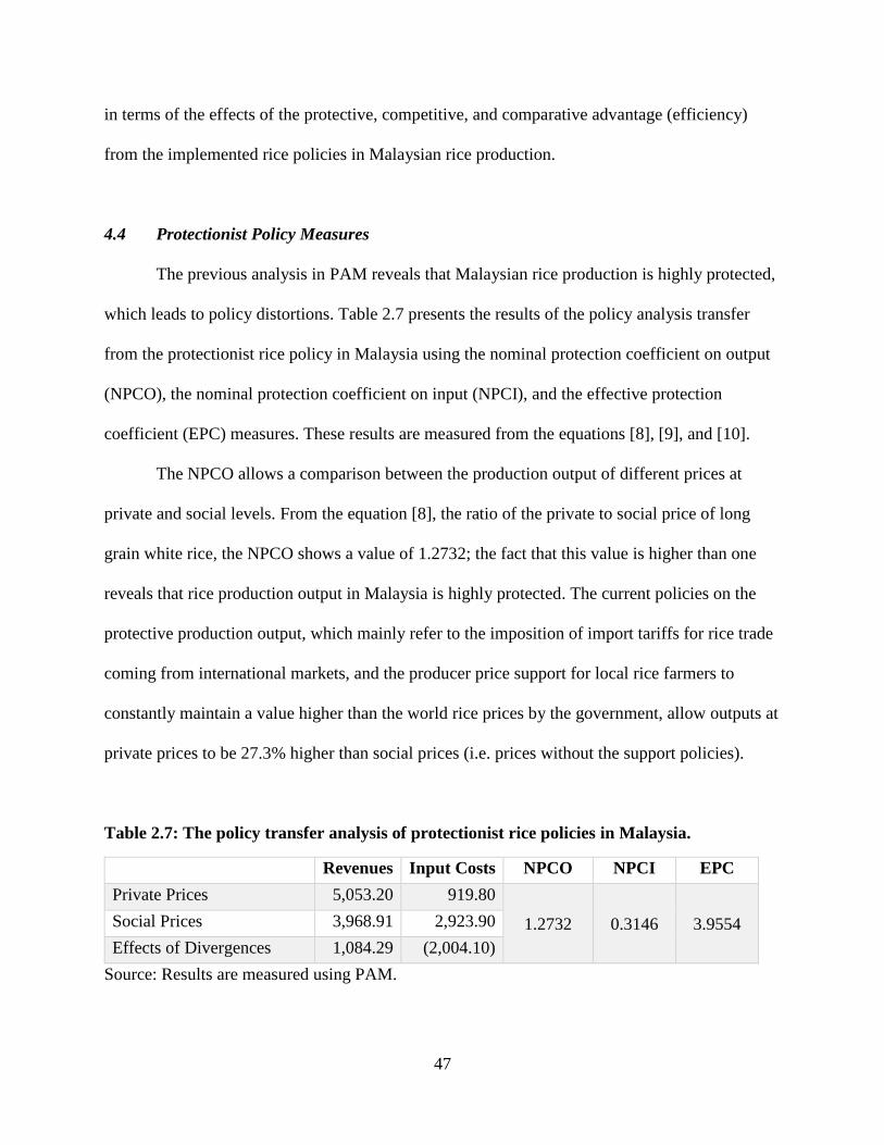
47
in terms of the effects of the protective, competitive, and comparative advantage (efficiency)
from the implemented rice policies in Malaysian rice production.
4.4 Protectionist Policy Measures
The previous analysis in PAM reveals that Malaysian rice production is highly protected,
which leads to policy distortions. Table 2.7 presents the results of the policy analysis transfer
from the protectionist rice policy in Malaysia using the nominal protection coefficient on output
(NPCO), the nominal protection coefficient on input (NPCI), and the effective protection
coefficient (EPC) measures. These results are measured from the equations [8], [9], and [10].
The NPCO allows a comparison between the production output of different prices at
private and social levels. From the equation [8], the ratio of the private to social price of long
grain white rice, the NPCO shows a value of 1.2732; the fact that this value is higher than one
reveals that rice production output in Malaysia is highly protected. The current policies on the
protective production output, which mainly refer to the imposition of import tariffs for rice trade
coming from international markets, and the producer price support for local rice farmers to
constantly maintain a value higher than the world rice prices by the government, allow outputs at
private prices to be 27.3% higher than social prices (i.e. prices without the support policies).
Table 2.7: The policy transfer analysis of protectionist rice policies in Malaysia.
Revenues Input Costs NPCO NPCI EPC
Private Prices 5,053.20 919.80
1.2732 0.3146 3.9554 Social Prices 3,968.91 2,923.90
Effects of Divergences 1,084.29 (2,004.10)
Source: Results are measured using PAM.

48
The NPCI measures the effects of distorting policies on tradable input costs in the rice
production system. The coefficient indicates a positive transfer of 0.3146 with the input
production costs are lowered by domestic subsidy support policies. This result implies that the
domestic policies reduce the input costs by 68.5% from the social price, causing the input costs
at private prices to be lower than social prices. Therefore, the input policies on domestic
production for seed, fertilizer, and pesticide cause policy distortion in a production system. With
the difference input costs of RM 2,004.1 (per hectare) which also refers to the current input
subsidies, rice farmers have to pay RM 919.8 (per hectare) for the input costs, rather than RM
2,923.9 (per hectare) with the absence of domestic support policies.
The different effects of output and input protection policies can be simultaneously
measured in the EPC coefficient. The EPC ratio of 3.95 represents the net impact of the input
and output policies affecting the rice production system. This result implies that both output and
input policies allow value added in private prices to be 295% higher than in social prices. The
result of EPC reveals that the highly protected outputs and inputs lead to a distorted Malaysian
rice production system.
The analysis of protection policy transfer for rice production policies in Malaysia reveals
that rice sector at farm level is highly distorted. Policy distortions in output and input markets are
complex to reconcile with the pursuit of economic competitive objectives, such as the self-
sufficiency goal (Vousden, 1990). As the government’s decision is to achieve rice self-
sufficiency, both input and output policies are heterogeneously distorted. These distortions
stimulate some unnecessary economic losses to achieve the goal of self-sufficiency. If the
government removes trade barriers on rice imports allowing free trade, the producer price would
decrease from the private to the social level. At this lower price, the country would increase rice

49
imports, decrease domestic production, and thus increase rice consumption. While rice import
prices are cheaper, the status quo forces consumers to pay a higher price for rice due to high
subsidization of domestic production. Hence, the protectionist policies lead the country to give
up potential gains from international trade.
4.5 Competitiveness and Efficiency Measures
With the PAM results, we can analyze the level of competitiveness and comparative
advantage which refers to the efficiency of the implemented rice policies. These measures are
analyzed using the domestic resource cost (DRC), the subsidy ratio to producer (SRP), and the
profitability coefficient (PC). These results are measured from the equations [11], [12], and [13],
shown in Table 2.8.
DRC is an important analysis which measures the efficiency of the entire a production
system as it serves as a proxy measure for social profits. The DRC coefficient indicates a value
greater than one (𝐷𝑅𝐶 > 1), 3.62, which demonstrates that Malaysia has no comparative
advantage in domestic rice production. Lacking international competitiveness, which currently
refers to the Vietnamese long grain white rice, the current protective rice policies are not
efficient. With the government’s policies continuing to emphasize domestic rice production to
achieve the self-sufficiency goal, mainly through largely subsidizing inputs and outputs, these
interventions would cause a significant inefficiency to the whole system of rice production.
Hence, the policy programs reflect sizable policy distortions.

50
Table 2.8: Measures of comparative advantage and competitiveness rice in Malaysia.
Revenues
Tradable
Input Costs
Domestic
Factors
Profits
DRC
SRP
Private Prices 5,053.20 919.80 3,430.04
703.36
3.6172
0.8663
Social Prices 3,968.91 2,923.90 3,780.04
(2,735.03)
Effects of
Divergences 1,084.29 (2,004.10) (350.00) 3,438.39
Source: Results are measured using PAM.
SRP measures net transfers across different systems of production as it allows for the
comparisons between policies which subsidize production systems, and gauges the
disaggregation into component transfers to show the distinct effects of policies on output, input,
and domestic factors. SRP shows a significantly high ratio at 0.8663 (close to one), meaning that
the divergences have highly distorted by the policies, which also means that gross revenues of
the production system are increased by 86.6%. This ratio shows the net transfers from
divergences largely result from social revenues. The ratio also implies that if policies on tradable
inputs and domestic factors are eliminated, the rice production system’s NPCO would have to be
increased from 1.27 to 1.86 to maintain the same degree of private profit.
4.6 Sensitivity Analysis
The main purpose of sensitivity analysis is to examine the efficiency of policy transfers
using the major analysis with changes in significant factors. Using the results of production
inputs and crop yield effects from the international free trade policy at the farm-household level
in Chapter IV, two scenarios are analyzed: 1) a decrease in production inputs by 16.2% and 2) a
decrease in rice yield by 4.8%. The results of sensitivity analysis are presented in Table 2.9. In
the first scenario, the DRC coefficient remains a value greater than one, 2.5061, which indicates
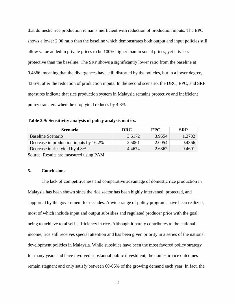
51
that domestic rice production remains inefficient with reduction of production inputs. The EPC
shows a lower 2.00 ratio than the baseline which demonstrates both output and input policies still
allow value added in private prices to be 100% higher than in social prices, yet it is less
protective than the baseline. The SRP shows a significantly lower ratio from the baseline at
0.4366, meaning that the divergences have still distorted by the policies, but in a lower degree,
43.6%, after the reduction of production inputs. In the second scenario, the DRC, EPC, and SRP
measures indicate that rice production system in Malaysia remains protective and inefficient
policy transfers when the crop yield reduces by 4.8%.
Table 2.9: Sensitivity analysis of policy analysis matrix.
Scenario DRC EPC SRP
Baseline Scenario 3.6172 3.9554 1.2732
Decrease in production inputs by 16.2% 2.5061 2.0054 0.4366
Decrease in rice yield by 4.8% 4.4674 2.6362 0.4601
Source: Results are measured using PAM.
5. Conclusions
The lack of competitiveness and comparative advantage of domestic rice production in
Malaysia has been shown since the rice sector has been highly intervened, protected, and
supported by the government for decades. A wide range of policy programs have been realized,
most of which include input and output subsidies and regulated producer price with the goal
being to achieve total self-sufficiency in rice. Although it barely contributes to the national
income, rice still receives special attention and has been given priority in a series of the national
development policies in Malaysia. While subsidies have been the most favored policy strategy
for many years and have involved substantial public investment, the domestic rice outcomes
remain stagnant and only satisfy between 60-65% of the growing demand each year. In fact, the

52
revised national rice policy provides additional input and output subsidies which burden
government expenditure while the government seriously pursues self-sufficiency approach and
aims to eliminate all rice imports in the near future. Therefore, it is crucial to evaluate and
analyze the competitiveness and the efficiency of domestic rice production as well as the effects
of policy transfer in the current Malaysian rice production system.
This study applies the policy analysis matrix (PAM) to measure the competitiveness and
comparative advantage of the rice sector in Malaysia. The data on a production level which
represents the costs of production and revenues in major producing areas is utilized. Prior to the
analysis, production budgets at private price and social price levels are established. Then, the
costs and revenues from the production budgets are applied to the PAM analysis to measure the
profitability and divergence effects at both price levels. Further, the analysis is extended to
measure the effects of the policy transfer. Despite having received substantial efforts and
attention by the government, especially through realizing various domestic support programs,
rice production in Malaysia suffers from comparative advantage relative to rice imports. The key
results indicate that rice policy in Malaysia is highly distorted, as number of policy programs,
that include subsidies, incentives, and price supports have raised private revenues and profits,
and thus lead to socially unprofitable rice production. In addition, the protection measures also
imply that the current policies are reducing the actual input costs while increasing the revenue
through subsidizing inputs and imposing higher domestic prices than market prices. The effects
of the divergences indicate that average rice farms generate a relatively low profit at private
prices while producing losses at social prices when the opportunity costs of all the domestic
factors involved in rice production are employed. The divergence is caused by government
policies that distort the pattern of production, moving it away from the most efficient use of

53
domestic resources and international trading opportunities. The competitiveness analysis proves
that the government’s decision in pursuing self-sufficiency through highly protecting the
domestic rice industry lead to significant market failures since the international rice price
(Vietnamese long grain white rice) is lower than local rice.
The government’s interventionist policy instruments significantly failed to drive
competitiveness in the Malaysian rice sector, hence leading to policy distortions. These
distortions induce unnecessary efficiency losses to realize the national self-sufficiency goal. The
government usually enacts distorting policies to favor particular interest groups, consciously
trading off the consequent efficiency losses against their perception of such non-efficiency gains
as changes in income distribution and improvement in the country’s ability to feed its nation.
With implementing protectionist policy, the government does not only distort the rice market,
but also each agricultural input market which include seed, fertilizer, pesticide, and other
chemicals. As rice in Malaysia is mostly operated by small farmers, it would be highly
challenging to become a competitive industry and would require significant financial support by
the government. This study provides key measures of the effects of rice policies on the
production system that could be a guideline for future policy decisions.
54
References
Abdullah, A. M., Mohamed Arshad, F., Radam, A., Ismail, M. M., Yacob, M.R., Harron, M.,
Mohamed, Z. A., Abd Latif, I., and Alias, E. F. 2010. Kajian Impak Skim Subsidi Baja
Padi Kerajaan Persekutuan (SSBPKP) dan Skim Subsidi Harga Padi (SSHP). Research
Report, Selangor: Universiti Putra Malaysia: Institut Kajian Dasar Pertanian dan
Makanan.
Adesina, A. A., and Coulibaly, O. N. 1998. Policy and Competitiveness of Agroforestry-Based
Technologies for Maize Production in Cameroon: An Application of Policy Analysis
Matrix. Agricultural Economics, 19 91-2).
Akramov, K., and Malek, M. 2012. Analyzing of Profitability of Maize, Rice, and Soybean
Production in Ghana: Results of PAM and DEA Analysis. Ghana Strategy Support
Program (GSSP) Working Paper No. 0028. IFPRI, USA.
Baharumshah, A. Z. 1991. "A Model for the Rice and Wheat Economy in Malaysia: An
Empirical Assessment of Alternative Specifications." PERTANIKA, 383 – 391.
Basavaraj, G., Rao, P., Achoth, L., and Reddy, C. 2013. Assessing Competitiveness of Sweet
Sorghum for Ethanol Production: A Policy Analysis Matrix Approach. Agricultural
Economics Research Review 26(1), 31 – 40.
Berita Harian. 2016. Discrepancy of Subsidies Payment– PAC, 10 November 2016.
Department of Agriculture, Malaysia. 2012-2013. Paddy Production Survey Report, Malaysia.
Dibrova, A. and Chan-Khi, O. 2013. Policy Analysis Matrix: An Analysis of the Effectiveness of
State Agricultural Policy for the Dairy Sector in Ukraine. Research in Agricultural
Economics and Applied Science, 13 (28).
Ekasingh, B., Surya, K., and Vutticharaenkarn, S. 2000. An Analysis of Land Use Systems
Using Policy Analysis Matrix (PAM) in a Small Watershed in Wat Chan, Northern
Thailand. Agricultural System Working Paper No. 134. Multiple Cropping Center,
Faculty of Agriculture, Chiang Mai University.
Elbadawi, E., Mohd Arshad, F., Mohamed, Z., and Ismail, M. 2013. Assessing Competitiveness
of Sheep Production in Selected States of Sudan. Journal of Agricultural Science, 5(1).
Canadian Center of Science and Education.

55
Fang, C., and John, C.B. 2000. Food Self-Sufficiency, Comparative, and Agricultural Trade: A
Policy Analysis Matrix for Chinese Agriculture. Center for Agricultural and Rural
Development Publications (CARD), Iowa States University.
Gotsch, C.G., Pearson, S.R., and Bahri, S. 2003. Computer Tutorial for Policy Analysis Matrix
in Indonesia, Agriculture Stanford University.
Kanaka, S. and Chinnadurai, M. 2013. The Policy Analysis Matrix of Rice Cultivation in India.
European Journal of Physical and Agricultural Sciences, 1 (1).
Khai, H., and Yabe, M. 2013. The Comparative Advantage of Soybean Production in Vietnam:
A Policy Analysis Matrix Approach. A Comprehensive Survey of International Soybean
Research - Genetics, Physiology, Agronomy and Nitrogen Relationships.
Khai, H. V., Yabe, M., Yokogawa, H., and Sato, G. 2008. The Situation and Comparative
Advantage of Soybean Production in the Mekong River Delta of Viet Nam, Journal of
the Faculty of Agriculture, Kyushu University, 53(2).
Kydd, J., Pearce, R., and Stockbridge, M. 1996. The Economic Analysis of Commodity Systems:
Extending the Policy Analysis Matrix to Account for Environmental Effects and
Transactions Costs, Agricultural Systems, 55(2).
Mstar. 2016. RM1.9 Billion for Subsidy and Incentives for 155,000 Rice Farmers.
http://www.mstar.com.my.
Mohd. Arshad, F., Mohayidin, M.G., Ayub, A.M., and Husin, M. 1983. The Impact of Paddy
Subsidy Schemes on Malaysian Farmers (in Malay). Consultancy Report, Kuala Lumpur:
Ministry of Public Enterprise, 421.
Mohamed Arshad, F., Raja Abdullah N., Kaur, B., and Abdullah, A. 2007. "50 Years of
Malaysian Agriculture: Transformational Issues, Challenges, and Direction. University
Putra Malaysia.
Mohamad Arshad, F. Mohayidin, M.G. 1990. Market Intervention in the Paddy and Rice
Industry: Evaluation, Rationale and Impact. Occasional Paper No. 6. Center for
Agricultural Policy Study, University Putra Malaysia, Serdang, Selangor.

56
Mohanty, S., Fang, C., and Chaudhary, J. 2003. Assessing the Competitiveness of Indian Cotton
Production: A Policy Analysis Matrix Approach, Journal of Cotton Science, 7(3).
Monke, E. and Pearson, S. 1989. The Policy Analysis Matrix for Agricultural Development.
Cornell University Press, Ithaca and London.
Mamza, A., Salman, K., and Adeoye, I. 2014. Competitiveness of Beef Processing in Borno
State of Nigeria: A Policy Matrix Analysis Approach. Journal of Agriculture and
Sustainability, 6(2), 132 – 147.
Mantau, Z., Harianto, and Nuriantono, N. 2014. Analysis of Competitiveness of Lowland Rice
Farming in Indonesia: Case Study of Bolaang Mongondow District, North Sulawesi
Province. Journal of Economics and International Finance, 6(4): 85 – 90.
Martinez, E., Picazo-Tadeo, A., and Estruch, V. 2008. The policy analysis matrix with profit-
efficient data: Evaluating profitability in rice cultivation. Spanish Journal of Agricultural
Research, 6 (3), 309 – 319.
Masters W., and Winter-Nelson A. 1995. Measuring the comparative advantage of agricultural
activities: Domestic resource costs and the social cost–benefit ratio. American Journal of
Agricultural Economics 77: 243–50.
Md Saiful Islam, A. and Kirschke, D. 2010. Protection and Comparative Advantage of Rice
Production in Bangladesh: A Policy Analysis Matrix. Himalayan Papers Research
Archive, Nepal Study Center, University of New Mexico, Albuquerque New Mexico.
Ministry of Agriculture and Agro-Based Industry. 2011-2014. National Agro-Food Policy 2011-
2020. Division of International and Strategic Planning. Putrajaya, Malaysia, ISBN: 978-
983-9863-41-3.
Nelson, G. C., and Panggabean, M. 1991. The Costs of Indonesian Sugar Policy: A Policy
Analysis Matrix Approach, American Journal of Agricultural Economics, 73(3).
New Straits Times. 2014. Malaysia Hopes to End Rice Imports By 2020. April 4.
Olowa, O. W. 2014. Remittances and Competition: A Policy Analysis Matrix Approach. Global
Journal of Management and Business Research: Economics and Commerce, 14 (4).
57
Overton, J. 1999. "Integration or Self-Sufficiency? Peninsular Malaysia and the Rice Trade in
Southeast Asia." Singapore Journal of Tropical Geography (Wiley Online Library) 20
(2): 169-180.
Pearson, S. R., Gotsch, C. G., and Bahri, S. 2003. Applications of the Policy Analysis Matrix in
Indonesian, Agriculture Stanford Unversity.
Pearson, S., Gotsch, C., and Bahri, S. 2004. Applications of Policy Analysis Matrix in
Indonesian Agriculture (Ed. 1). Yayasan Obor Indonesia.
Pearson, S., Monke, E., Argwings-Kodhek, G., Avillez, F., Mukumbu, M., Stefano, P., Sellen,
D., and Winter-Nelson. 1995. Agricultural Policy in Kenya: Applications of the Policy
Analysis Matrix. Cornell University Press, Ithaca and London.
Rae, A., and Kasryno, F. 1993. A PAM Analysis of Livestock in Indonesia Policies. Agricultural
and Resource Economics Review, 22 (1): 59 – 70.
Scarborough, V., and Kydd, J. G. 1992. Economic Analysis of Agricultural Markets: a Manual,
NRI Marketing Series, 5, Chatham.
Staal, S. J., Shapiro, B. I. 1994. The effects of recent price liberalization on Kenyan peri-urban
dairy. A case study using the policy analysis matrix approach, Food Policy, 19 (6).
Suleiman, U. H., Abdullah, A.M., Shamsudin, M.N., and Mohamed, Z.A. (2014). Effects of
Paddy Price Support Withdrawal on Malaysian Rice Sector: Time Series Econometric
Approach. Asian Journal of Agriculture and Rural Development, 4(7):401-413,
Department of Agribusiness and Information System; Faculty of Agriculture, University
Putra Malaysia, Serdang Selangor, Malaysia.
Ude, M., Adeoye, I., Yusuf, S., Balogun, O., and Akinlade, R. 2013. Competitiveness of Rice
Processing and Marketing in Ebonyi State: A Policy Analysis Matrix Approach.
International Journal of Agricultural Sciences, 3(2): 410 – 418.
United Nation. 2014. UN Comtrade Database. www. un.org.

58
Ugochukwu, A., and Ezedinma, C. 2011. Intensification of Rice Production Systems in
Southeastern Nigeria: A Policy Analysis Matrix Approach. International Journal of
Agricultural Management & Development (IJAMAD), 1(2): 89 – 100.
Vengedasalam, D., Harris, M., and MacAulay, G. 2011. "Malaysian Rice Trade and Government
Interventions." 55th Annual Conference of Australian Agricultural and Resource
Economic Society.
Vousden, N. 1990. The Economics of Trade Protection. Cambridge University Press, United
Kingdom
Yao, S. 1997. Rice Production in Thailand Seen Through a Policy Analysis Matrix. Food Policy,
22 (2), 547 – 560. Elsevier Science Ltd.
Zheng, S., Lambert, D., Wang, S., and Wang, Z. 2013. Effects of Agricultural Subsidy Policies
on Comparative Advantage and Production Protection in China: An Application with a
Policy Analysis Matrix Model. The Chinese Economy, 46 (1): 20 – 37.

59
Appendix Table 2.1: Physical input and output of rice production system in Malaysia.
Input-Output Items Amount/Ha
Tradable Inputs
Seed (kg) 150.0
Fertilizers:
Urea (kg) 80.0
NPK (kg) 240.0
Organic (kg) or 100.0
Foliar (liter) 6.0
Ground Magnesium Limestone (GML) (mt) 3.0
Additional NPK (kg) 150.0
Chemicals:
Herbicide
Basta (Liter) 4.0
Clincher (mililiter) 500.0
Sindex (gram) 1,000.0
Insecticide
Evisect (kg) 1.0
Confidor (mililiter) 500.0
Actara (gram) 600.0
Fungicide
Score 250L (mililiter) 250.0
Fujicone (liter) 1.0
Pesticide
Matikus (kg) 18.0
Irrigation and drainage (M3) 277.0
Soil fertility - GML (RM/ha) 250.0
Rice straw cleaning (RM/ha) 78.0
Plowing (RM/ha) 220.0
Irrigation and drainage (RM/ha) 150.0
Rice-field mice control (RM/ha) 20.0
Weed control (before planting) (RM/ha) 50.0
Seed sowing (RM/ha) 50.0
Weed control (after planting) (RM/ha) 150.0

60
Appendix Table 2.1 (Cont.)
Input-Output Items Amount/Ha
Domestic Factors
Replanting (RM/ha) 80.0
Preparing working tracks (RM/ha) 80.0
Pest and disease control (RM/ha) 150.0
Fertilizing (RM/ha) 200.0
Weedy rice control (RM/ha) 300.0
Harvesting (RM/ha) 500.0
Capital:
Tractor services (RM/ha) 300.0
Land (ha) 1.0
Output Yield (paddy basis, dried and cleaned) (Mt/ha) 4.21
Source: DOA; LPP.
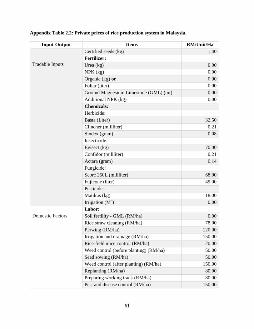
61
Appendix Table 2.2: Private prices of rice production system in Malaysia.
Input-Output Items RM/Unit/Ha
Tradable Inputs
Certified seeds (kg) 1.40
Fertilizer:
Urea (kg) 0.00
NPK (kg) 0.00
Organic (kg) or 0.00
Foliar (liter) 0.00
Ground Magnesium Limestone (GML) (mt) 0.00
Additional NPK (kg) 0.00
Chemicals:
Herbicide:
Basta (Liter) 32.50
Clincher (mililiter) 0.21
Sindex (gram) 0.08
Insecticide:
Evisect (kg) 70.00
Confidor (mililiter) 0.21
Actara (gram) 0.14
Fungicide:
Score 250L (mililiter) 68.00
Fujicone (liter) 49.00
Pesticide:
Matikus (kg) 18.00
Irrigation (M3) 0.00
Domestic Factors
Labor:
Soil fertility - GML (RM/ha) 0.00
Rice straw cleaning (RM/ha) 78.00
Plowing (RM/ha) 120.00
Irrigation and drainage (RM/ha) 150.00
Rice-field mice control (RM/ha) 20.00
Weed control (before planting) (RM/ha) 50.00
Seed sowing (RM/ha) 50.00
Weed control (after planting) (RM/ha) 150.00
Replanting (RM/ha) 80.00
Preparing working track (RM/ha) 80.00
Pest and disease control (RM/ha) 150.00

62
Appendix Table 2.2 (Cont.)
Input-Output Items RM/Unit/Ha
Domestic Factors
Fertilizing (RM/ha) 200.00
Weedy rice control (RM/ha) 300.00
Harvesting (RM/ha) 500.00
Capital:
Tractor services (RM/ha) 300.00
Land rental (RM/ha) 1,202.04
Output
Producer price support policy (paddy basis;
dried and cleaned) (RM/Mt) 1,200.00
Source: DOA; LPP.

63
Appendix Table 2.3: Social prices of rice production system in Malaysia.
Input-Output Items RM/Unit/Ha
Tradable Inputs
Seed (RM/kg) 2.43
Fertilizer:
Urea (kg) 1.15
NPK (kg) 2.26
Organic (kg) or 1.21
Foliar (liter) 20.40
Ground Magnesium Limestone (GML) (mt) 240.00
Additional NPK (kg) 2.70
Chemicals:
Herbicide:
Basta (Liter) 32.50
Clincher (mililiter) 0.21
Sindex (gram) 0.08
Insecticide:
Evisect (kg) 70.00
Confidor (mililiter) 0.21
Actara (gram) 0.14
Fungicide:
Score 250L (mililiter) 68.00
Fujicone (liter) 49.00
Pesticide:
Matikus (kg) 18.00
Irrigation and drainage (M3) 0.90
Domestic Factors
Labor:
Soil fertility - GML (RM/ha) 250.00
Rice straw cleaning (RM/ha) 78.00
Plowing (RM/ha) 220.00
Irrigation and drainage (RM/ha) 150.00
Rice-field mice control (RM/ha) 20.00
Weed control (before planting) (RM/ha) 50.00
Seed sowing (RM/ha) 50.00
Weed control (after planting) (RM/ha) 150.00
Replanting (RM/ha) 80.00
Preparing working track (RM/ha) 80.00
Pest and disease control (RM/ha) 150.00
Fertilizing (RM/ha) 200.00

64
Appendix Table 2.3 (Cont.)
Input-Output Items RM/Unit/Ha
Domestic Factors
Weedy rice control (RM/ha) 300.00
Harvesting (RM/ha) 500.00
Capital:
Tractor services (RM/ha) 300.00
Land rental (RM/ha) 1,202.04
Output Import parity value at farm gate (RM/Mt) 942.51
Source: DOA; LPP.

65
Chapter III
Self-sufficiency and International Trade Policies on Rice Sector in Malaysia: Approaches
to Food Security using Partial Equilibrium Analysis
Abstract
While much evidence shows self-sufficiency is not an efficient policy strategy to address
food security concerns as well as poverty alleviation, Malaysia is following a self-sufficiency
strategy in its primary staple, rice. This study evaluates and analyzes the impact of two
alternative approaches to achieve food security, namely, pursuing rice self-sufficiency, and
allowing free trade in rice. The results indicate that even though Malaysia could achieve self-
sufficiency in rice, consumers are worse off, since consumer rice prices increase sharply. On the
other hand, rice producers are better off due to higher producer prices and domestic production.
The government welfare worsens from the self-sufficiency policy due to massive requirements
on additional subsidies and the loss of import tariff revenues. Free trade results in lower
consumer prices and greater rice consumption, thus favoring consumer welfare. Producer welfare
worsens due to higher import competition and lower producer prices. With a long-held food
security rationale, rice self-sufficiency neither guarantees nor promises food security in
Malaysia. Pursuing self-sufficiency would effectively punish consumers, and even the
government loses from the policy. Otherwise, self-sufficiency could also be a political strategy in
political economic environment to become an independent region without relying on external
food sources. This study provides useful economic insights to the government and policymakers
on self-sufficiency and free trade assessments for policy direction of rice sector in Malaysia.

66
1. Introduction
Self-sufficiency has been brought to the world’s attention and has moved to the higher
policy agenda particularly to address food security concerns in most rice-staple and rice-deficit
regions among developing countries. Despite the criticism for not being an efficient approach,
self-sufficiency has been promoted and adopted as the pertinent solution to achieve food security
objectives, especially in the aftermath of the recent global food crisis (FAO, 2016). Malaysia
announced its intention to pursue self-sufficiency by the year 2020 and has recently been
extended to the year 2050 (National Transformation 2020-2050). The pursue of self-sufficiency
is not only for food security reasons, but also the result of a political economy that prioritizes
farmers’ interests and strives to guarantee the welfare of rice farmers. Since the majority of rice
farmers are poor smallholders, self-sufficiency may help ameliorate poverty among farmers.
Food self-sufficiency is not a new policy strategy in Malaysia as the country has historically
focused on supported domestic rice production to obtain a high degree self-sufficiency. As
domestic demand for rice is growing, self-sufficiency goals become more challenging (Figure
3.8). Intensification of rice production has been one way to improve land productivity and
output. Currently the crop intensity of rice is considerably high, ranging between 170% and
180%, yet domestic production remains constrained by its marginal productivity (Mailena et al.,
2014). The expansion of rice acreage is highly constrained in Malaysia. Most arable land in
Malaysia is under permanent palm oil and rubber crops. Pursuing self-sufficiency with a
constrained supply of land requires significant gains in productivity or otherwise will lead to
higher market prices, and consequently reduced consumer welfare.

67
Source: Production, Supply and Distribution (PS&D), USDA.
Figure 3.8: Trends of domestic demand and self-sufficiency ratio for rice in Malaysia,
1960 – 2016.
Even if food self-sufficiency and food security are interconnected, the government’s
stance on self-sufficiency is misconstrued while often interpreting to food security. According to
the Food and Agricultural Organization (FAO), food self-sufficiency is referred to “The extent to
which a country can satisfy its food needs from its own domestic production”, “Closing borders
adopting complete autarky for food sector, and “A country producing sufficient food to cover its
own needs” (Clapp, 2017; FAO, 2016; FAO, 1999) (Figure 3.9). Food security, on the other
hand, pertains to food availability, accessibility, nutrition, and stability across the three
dimensions (FAO, 2008). As such, food security makes no reference to the source of food
(Clapp, 2014), and therefore food security and self-sufficiency are divergent and express
different concepts. The World Bank stressed that ‘‘Food self-sufficiency should be weighed
against the benefits of cheaper imports” (World Bank, 2012). In fact, self-sufficiency has also
0.0
10.0
20.0
30.0
40.0
50.0
60.0
70.0
80.0
90.0
100.0
0
500
1,000
1,500
2,000
2,500
3,000
19
60
19
63
19
66
19
69
19
72
19
75
1978
1981
1984
1987
1990
19
93
19
96
19
99
20
02
20
05
20
08
20
11
20
14
Domestic Demand Self-sufficiency Ratio
MT %

68
been claimed as outcomes when a country prioritizes political decisions over economic rationale
in food policy choices which characterize by conflict between interests that support local
production and those that believe self-sufficiency is a costlier path and thus worsens public
investments (Clapp, 2017).
Source: Clapp (2017)
Figure 3.9: The concept of food self-sufficiency.
Self-sufficiency has been criticized because it embraces policies which are being
inefficient and distort the market resulting in weakened incentives for food production, thus
leading to higher food prices in the long run (Naylor and Falcon, 2010). Strongly emphasizing to
the self-sufficiency goal diverts government’s attention from pressing food security concerns at
the household level (Von Braun and Paulino, 1990). Other countries are also discovering that
self-sufficiency is more likely to cause negative consequences (Mosavi and Esmaeili, 2012).
Food Consumed
Food
Pro
du
ced
Countries above
the line produced
more food than
they consumed
Countries below
the line
consumed
more food than
they produced

69
Instead, liberalizing food trade shows many advantages to improve food security as well
as economic growth, especially for developing economic regions. Many developing countries
realized that the free trade was an effective approach for sustained development. For instance,
Latin America and East Asia indicated significant economic development growth in 1985 to
2005 when practicing the free trade (OECD, 2008), and thus there were positive relationships
between free trade and economic growth (Von Braun and Diaz-Bonilla, 2008). The World Bank
reviewed many studies regarding globalizing trade to poverty reduction and concluded that the
degree of trade openness played a significant role and benefited certain countries to better
integrate into the world economy (World Bank, 2002). In fact, a rice import tariff will not help
local producers, and even punish local consumers (Jolly et al., 2009).
Malaysia has been active participating free trade agreements (FTAs) in both bilateral and
regional levels and is currently involved in 13 FTAs as well as a member of the World Trade
Organization (WTO) (Table 3.10). Nevertheless, Malaysia has excluded rice in the FTAs and
declared as a sensitive product, which allows it to extend protection to local rice industry. Under
ASEAN13-Australia-New Zealand Regional Free Trade Agreement, rice remains excluded from
Malaysia’s tariff commitments until 2023, when its tariff will be bound at 30% and then reduced
annually until it is eliminated in 2026 (Malaysian Ministry of International Trade and Industry,
2006).
13 The Association of Southeast Asian Nations (ASEAN) was formed to promote political and
economic cooperation and regional stability which is currently participated by 10-member
countries – Malaysia, Indonesia, Singapore, Brunei, Vietnam, Thailand, Philippines, Cambodia,
Myanmar, and Laos.

70
Table 3.10: Malaysia: Current bilateral and regional free trade agreements (FTAs).
Free Trade Agreements Participating
Date
Bilateral
Malaysia-Japan Economic Partnership Agreement (MJEPA) 13 July 2006
Malaysia-Pakistan Closer Economic Partnership Agreement
(MPCEPA) 1 Jan. 2008
Malaysia-New Zealand Free Trade Agreement (MNZFTA) 1 Aug. 2010
Malaysia-India Comprehensive Economic Cooperation
Agreement (MICECA) 1 July 2011
Malaysia-Chile free Trade Agreement (MCFTA) 25 Feb. 2012
Malaysia-Australia free Trade Agreement (MAFTA) 1 Jan. 2013
Malaysia-Turkey Free Trade Agreement (MTFTA) 1 Aug. 2015
Regional
ASEAN-China Free Trade Agreement (ACFTA) 1 July 2003
ASEAN-Korea Free Trade Agreement (AKFTA) 1 July 2006
ASEAN-Japan Comprehensive Economic Partnership (AJCEP) 1 Feb. 2009
ASEAN-Australia-New Zealand Free Trade Agreement
(AANZFTA) 1 Jan. 2010
ASEAN-India Free Trade Agreement (AIFTA) 1 Jan. 2010
ASEAN Trade in Goods Agreement (ATIGA) 17 May 2010
Source: Ministry of International Trade and Industry, Malaysia.
Despite the substantial government’s efforts to expand the areas in which rice is grown,
upgrading technologies and research and development, developing and maintaining
infrastructures, and investing in subsidy and incentive programs, the domestic production is still
insufficient, covering between 60 – 65% of the total domestic demand. Malaysia has been a net
rice importer for many years, depending on rice imports to satisfy the required domestic demand.
Our projections to 2020 still suggest a significant reliance on imports (Figure 3.10). Therefore,
the government’s decision to eliminate rice trades is pondered as an extreme policy strategy as
Malaysia is not competitive in rice production (see Chapter II). Using a massive public
investment and implicitly taxpayers’ dollars to support a highly subsidized crop in order to
achieve self-sufficiency goal, it is crucial to evaluate the policies and analyze the impact of a
long-held policy strategy at the macro level.

71
Source: RICEFLOW Database.
Figure 3.10: Bilateral rice trades (in Thousand Mt) from Malaysian trading partners.
From the discussion above, some of the overarching questions this study attempts to
answer includes: 1) What are the consequences of enforcing a total rice self-sufficiency? 2) What
are the main limitations to achieve the self-sufficiency?, and 3) Is rice self-sufficiency an
efficient approach to pursue? Subsequently, the main objective of this study is to evaluate and
analyze the impacts of rice self-sufficiency, as an alternative, international free trade in Malaysia.
The specific objectives are:
1) To simulate the impacts of self-sufficiency policy on total rice output and consumption.
2) To estimate the subsidy and production input requirements to achieve rice self-sufficiency.
3) To measure the government’s potential gains or losses from rice self-sufficiency.
4) To assess the effects of removing rice trade restrictions on rice production and consumption.
0
100
200
300
400
500
600
Vietnam Thailand Pakistan Cambodia India Myanmar United
States
ROW
Vietnam Thailand Pakistan Cambodia India MyanmarUnited
StatesROW
2013-15 493.15 336.38 126.81 48.48 36.67 3.9 1.22 0.46
2020 579.00 373.20 139.78 52.89 33.20 3.73 1.38 0.53

72
This study utilizes a spatial partial equilibrium model of the global rice economy to
simulate two main policy scenarios; 1) rice self-sufficiency in Malaysia, and 2) the complete
removal of import tariffs on rice in Malaysia. The self-sufficiency policy scenario is simulated
by eliminating Malaysia’s bilateral import volume, while the free trade is simulated by removing
existing import tariffs affecting rice imports in Malaysia. Prior to the simulation analysis, a
baseline for the year 2020 is established to be consistent with the policy goal timelines, and
therefore the results would be more realistic and representative. From self-sufficiency scenarios,
we further estimate the policy requirements on subsidy, production input, technology efficiency,
and the government potential revenues and losses.
2. Materials and Methods
2.1 Modeling Framework
This study applies a spatial partial equilibrium model of the global rice economy
(Durand-Morat and Wailes, 2010). The model simulates the behavior of the entire rice supply
chain, from input markets all the way up to the aggregate final demand, in multiple
countries/regions (set 𝑅) around the world. Production of endogenous rice commodities (set
𝐶𝐸14) is specified as a weak-separable, constant return to scale production function.
𝑌𝑐,𝑟 = 𝐻𝑐,𝑟{𝐺𝑐,𝑟(𝐹𝐴𝐶𝑐,𝑟), 𝐼𝑁𝑇𝑐,𝑟} ∀𝑐 ∈ 𝐶𝐸, 𝑟 ∈ 𝑅 [1]
14 𝐶𝐸 = {𝐿𝐺𝑃, 𝐿𝐺𝐵, 𝐿𝐺𝑊, 𝑀𝐺𝑃, 𝑀𝐺𝐵, 𝑀𝐺𝑊, 𝐹𝑅𝑃, 𝐹𝑅𝐵, 𝐹𝑅𝑊}, where LG, MG, and FR stand
for long grain, medium/short grain, and fragrant rice, and P, B, W stand for paddy/rough,
brown/whole, and white/milled rice.

73
Where 𝑌 represents output, 𝐻 and 𝐺 are technology functional forms, 𝐹𝐴𝐶15 is the set of factors
of production, and 𝐼𝑁𝑇16 is the set of intermediate inputs.
Defining 𝐺 in [1] as a constant elasticity of substitution (CES) function, the derived
demand for factor of production, 𝑄𝐹𝐶, is:
𝑄𝐹𝐶𝑓,𝑐,𝑟 ∗ 𝐴𝐹𝐶𝑓,𝑐,𝑟 = 𝑄𝑉𝐴𝑐,𝑟 ∗ 𝑆𝑉𝐴𝑓,𝑐,𝑟 ∗ [𝑃𝐹𝐶𝑓,𝑐,𝑟
𝑃𝑉𝐴𝑐,𝑟∗𝐴𝐹𝐶𝑓,𝑐,𝑟]
−𝜎𝑉𝐴𝑐,𝑟
∀𝑓 ∈ 𝐹𝐴𝐶, 𝑐 ∈ 𝐶𝐸, 𝑟 ∈ 𝑅 [2]
𝑃𝑉𝐴𝑐,𝑟 = [∑ 𝑆𝑉𝐴𝑓,𝑐,𝑟 ∗ (𝑃𝐹𝐶𝑓,𝑐,𝑟
𝐴𝐹𝐶𝑓,𝑐,𝑟)
1−𝜎𝑉𝐴𝑐,𝑟
𝑓
]
11−𝜎𝑉𝐴𝑐,𝑟
∀𝑐 ∈ 𝐶𝐸, 𝑟 ∈ 𝑅 [3]
Where 𝐴𝐹𝐶, 𝑃𝐹𝐶, and 𝑆𝑉𝐴 are a factor-, sector-, and region-specific augmenting technical
change variable, factor price variable, and cost share in value added, respectively, and 𝑄𝑉𝐴 and
𝑃𝑉𝐴 are a sector- and region-specific derived demand and price for the value-added composite,
respectively. Finally, 𝜎𝑉𝐴 is the sector- and region-specific elasticity of substitution in value-
added.
15 𝐹𝐴𝐶 = {𝐿, 𝑇, 𝐾}, where 𝐿 is land, 𝑇 labor, and 𝐾 capital.
16 𝐼𝑁𝑇 = {𝑠𝑒𝑒𝑑𝑠, ℎ𝑒𝑟𝑏𝑐𝑖𝑑𝑒𝑠, 𝑝𝑒𝑠𝑡𝑖𝑐𝑖𝑑𝑒𝑠, 𝑤𝑎𝑡𝑒𝑟, 𝑒𝑛𝑒𝑟𝑔𝑦, 𝐿𝐺𝑃, 𝐿𝐺𝐵, 𝑀𝐺𝑃, 𝑀𝐺𝐵, 𝐹𝑅𝑃, 𝐹𝑅𝐵}
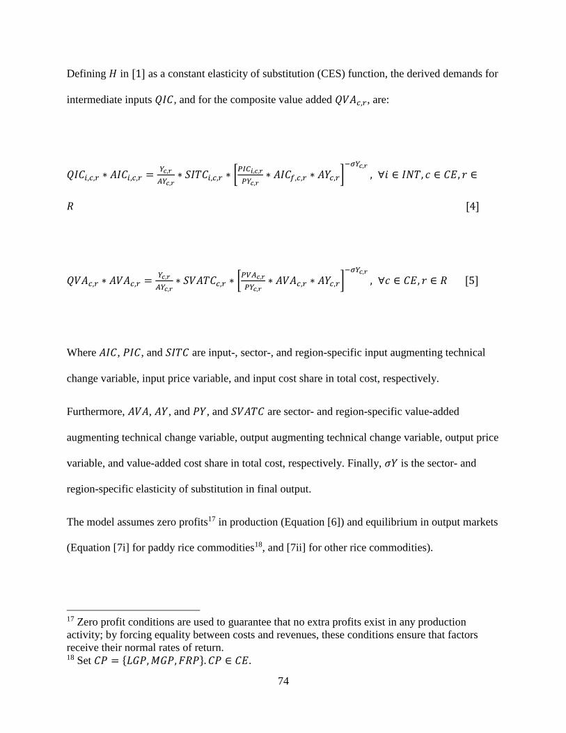
74
Defining 𝐻 in [1] as a constant elasticity of substitution (CES) function, the derived demands for
intermediate inputs 𝑄𝐼𝐶, and for the composite value added 𝑄𝑉𝐴𝑐,𝑟, are:
𝑄𝐼𝐶𝑖,𝑐,𝑟 ∗ 𝐴𝐼𝐶𝑖,𝑐,𝑟 =𝑌𝑐,𝑟
𝐴𝑌𝑐,𝑟∗ 𝑆𝐼𝑇𝐶𝑖,𝑐,𝑟 ∗ [
𝑃𝐼𝐶𝑖,𝑐,𝑟
𝑃𝑌𝑐,𝑟∗ 𝐴𝐼𝐶𝑓,𝑐,𝑟 ∗ 𝐴𝑌𝑐,𝑟]
−𝜎𝑌𝑐,𝑟
, ∀𝑖 ∈ 𝐼𝑁𝑇, 𝑐 ∈ 𝐶𝐸, 𝑟 ∈
𝑅 [4]
𝑄𝑉𝐴𝑐,𝑟 ∗ 𝐴𝑉𝐴𝑐,𝑟 =𝑌𝑐,𝑟
𝐴𝑌𝑐,𝑟∗ 𝑆𝑉𝐴𝑇𝐶𝑐,𝑟 ∗ [
𝑃𝑉𝐴𝑐,𝑟
𝑃𝑌𝑐,𝑟∗ 𝐴𝑉𝐴𝑐,𝑟 ∗ 𝐴𝑌𝑐,𝑟]
−𝜎𝑌𝑐,𝑟
, ∀𝑐 ∈ 𝐶𝐸, 𝑟 ∈ 𝑅 [5]
Where 𝐴𝐼𝐶, 𝑃𝐼𝐶, and 𝑆𝐼𝑇𝐶 are input-, sector-, and region-specific input augmenting technical
change variable, input price variable, and input cost share in total cost, respectively.
Furthermore, 𝐴𝑉𝐴, 𝐴𝑌, and 𝑃𝑌, and 𝑆𝑉𝐴𝑇𝐶 are sector- and region-specific value-added
augmenting technical change variable, output augmenting technical change variable, output price
variable, and value-added cost share in total cost, respectively. Finally, 𝜎𝑌 is the sector- and
region-specific elasticity of substitution in final output.
The model assumes zero profits17 in production (Equation [6]) and equilibrium in output markets
(Equation [7i] for paddy rice commodities18, and [7ii] for other rice commodities).
17 Zero profit conditions are used to guarantee that no extra profits exist in any production
activity; by forcing equality between costs and revenues, these conditions ensure that factors
receive their normal rates of return. 18 Set 𝐶𝑃 = {𝐿𝐺𝑃, 𝑀𝐺𝑃, 𝐹𝑅𝑃}. 𝐶𝑃 ∈ 𝐶𝐸.
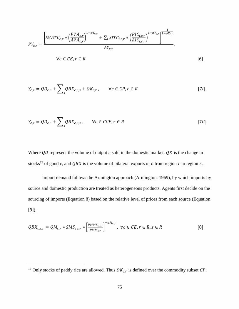
75
𝑃𝑌𝑐,𝑟 =
[𝑆𝑉𝐴𝑇𝐶𝑐,𝑟 ∗ (𝑃𝑉𝐴𝑐,𝑟
𝐴𝑉𝐴𝑐,𝑟)
1−𝜎𝑌𝑐,𝑟
+ ∑ 𝑆𝐼𝑇𝐶𝑖,𝑐,𝑟 ∗ (𝑃𝐼𝐶𝑖,𝑐,𝑟
𝐴𝐼𝐶𝑖,𝑐,𝑟)
1−𝜎𝑌𝑐,𝑟
𝑖 ]
11−𝜎𝑌𝑐,𝑟
𝐴𝑌𝑐,𝑟,
∀𝑐 ∈ 𝐶𝐸, 𝑟 ∈ 𝑅 [6]
𝑌𝑐,𝑟 = 𝑄𝐷𝑐,𝑟 + ∑ 𝑄𝐵𝑋𝑐,𝑟,𝑠𝑠
+ 𝑄𝐾𝑐,𝑟 , ∀𝑐 ∈ 𝐶𝑃, 𝑟 ∈ 𝑅 [7𝑖]
𝑌𝑐,𝑟 = 𝑄𝐷𝑐,𝑟 + ∑ 𝑄𝐵𝑋𝑐,𝑟,𝑠𝑠
, ∀𝑐 ∈ 𝐶𝐶𝑃, 𝑟 ∈ 𝑅 [7𝑖𝑖]
Where 𝑄𝐷 represent the volume of output 𝑐 sold in the domestic market, 𝑄𝐾 is the change in
stocks19 of good c, and 𝑄𝐵𝑋 is the volume of bilateral exports of 𝑐 from region 𝑟 to region 𝑠.
Import demand follows the Armington approach (Armington, 1969), by which imports by
source and domestic production are treated as heterogeneous products. Agents first decide on the
sourcing of imports (Equation 8) based on the relative level of prices from each source (Equation
[9]).
𝑄𝐵𝑋𝑐,𝑠,𝑟 = 𝑄𝑀𝑐,𝑟 ∗ 𝑆𝑀𝑆𝑐,𝑠,𝑟 ∗ [𝑃𝑀𝑀𝑆𝑐,𝑠,𝑟
𝑃𝑀𝑀𝑐,𝑟]
−𝜎𝑀𝑐,𝑟
, ∀𝑐 ∈ 𝐶𝐸, 𝑟 ∈ 𝑅, 𝑠 ∈ 𝑅 [8]
19 Only stocks of paddy rice are allowed. Thus 𝑄𝐾𝑐,𝑟 is defined over the commodity subset 𝐶𝑃.
76
𝑃𝑀𝑀𝑐,𝑟 = [∑ 𝑆𝑀𝑆𝑐,𝑠,𝑟 ∗ 𝑃𝑀𝑀𝑆𝑐,𝑠,𝑟1−𝜎𝑀𝑐,𝑟
𝑠
]
11−𝜎𝑀𝑐,𝑟
, ∀𝑐 ∈ 𝐶𝐸, 𝑟 ∈ 𝑅 [9]
Where 𝑃𝑀𝑀𝑆 is the market price of import good 𝑐 into region 𝑟 from source 𝑠, 𝑃𝑀𝑀 is the
composite market price of import good 𝑐 in 𝑟, 𝑄𝑀 is the demand for the composite import good
𝑐 in 𝑟, and 𝑆𝑀𝑆 is the value-share of good 𝑐’s imports into 𝑟 by source 𝑠. 𝜎𝑀𝑐,𝑟 is the elasticity
of substitution of imported good 𝑐 in 𝑟 by source.
After sourcing imports, then agents decide on the optimal mix of imported and domestic
products (Equation [10] and [11]) based on their relative price levels (Equation [12]).
𝑄𝑀𝑐,𝑟 = 𝑄𝑄𝑐,𝑟 ∗ 𝑆𝑀𝑄𝑐,𝑟 ∗ [𝑃𝑀𝑀𝑐,𝑟 𝑃𝑄𝑐,𝑟⁄ ]−𝜎𝑄𝑐,𝑟
, ∀𝑐 ∈ 𝐶𝐸, 𝑟 ∈ 𝑅 [10]
𝑄𝐷𝑐,𝑟 = 𝑄𝑄𝑐,𝑟 ∗ 𝑆𝐷𝑄𝑐,𝑟 ∗ [𝑃𝑌𝑐,𝑟 𝑃𝑄𝑐,𝑟⁄ ]−𝜎𝑄𝑐,𝑟
, ∀𝑐 ∈ 𝐶𝐸, 𝑟 ∈ 𝑅 [11]
𝑃𝑄𝑐,𝑟 = [𝑆𝑀𝑄𝑐,𝑟 ∗ 𝑃𝑀𝑀𝑐,𝑟1−𝜎𝑄𝑐,𝑟 + 𝑆𝐷𝑄𝑐,𝑟 ∗ 𝑃𝑌𝑐,𝑟
1−𝜎𝑄𝑐,𝑟]1
1−𝜎𝑄𝑐,𝑟 , ∀𝑐 ∈ 𝐶𝐸, 𝑟 ∈ 𝑅 [12]
Where 𝑃𝑄 is the market price of composite good 𝑐 in region 𝑟, 𝑄𝑄 is the output of composite
good 𝑐 in 𝑟, and 𝑆𝑀𝑄 and SDQ are the value-shares of the import composite and domestic good
𝑐 in 𝑟. 𝜎𝑄𝑐,𝑟 is the elasticity of substitution between domestic and imported good 𝑐 in 𝑟.

77
Final demand for milled rice 𝑐 ∈ 𝐶𝐹𝐶20 in region 𝑟, is the product of population and per-
capita demand 𝐷𝑐,𝑟, which is specified as a double log function of income and prices (Equation
[13]). 𝑍𝑟 represents income by region, 𝜑𝑟 is the income demand elasticity, and 𝜔𝑐,𝑔,𝑟 is the
matrix of own and cross-price demand elasticities.
log 𝐷𝑐,𝑟 = 𝜑𝑟 ∗ log 𝑍𝑟 + ∑ 𝜔𝑐,𝑔,𝑟 ∗ log 𝑃𝑄𝑔,𝑟𝑔 ∈ 𝐹𝐶 , ∀𝑐 ∈ 𝐶𝐹𝐶, 𝑟 ∈ 𝑅 [13]
The supply of exogenous intermediate inputs (seeds, fertilizers, pesticides, energy, and water),
capital, and labor are specified as perfectly elastic, thus their prices (𝑃𝐹𝐶) are treated as constant,
exogenous variables. Land is considered the only factor with limited supply. Hence, sectoral
output 𝑌 is constrained only by the supply of land 𝐿𝑐,𝑟 used in the production of paddy rice,
which is represented by a double log function of land rental rates 𝑃𝐿𝑐,𝑟.
log 𝐿𝑐,𝑟 = 𝜃𝑐,𝑟 log 𝑃𝐿𝑐,𝑟 , ∀𝑐 ∈ 𝐶𝑃, 𝑟 ∈ 𝑅 [15]
The land own-price supply elasticity 𝜃𝑐,𝑟 are calibrated following Keller (1976) to reflect rice
supply elasticities found in the literature.
20 Set 𝐶𝐹𝐶 = {𝐿𝐺𝑊, 𝑀𝐺𝑊, 𝐹𝑅𝑊}. 𝐶𝐹𝐶 ∈ 𝐶𝐸.
78
2.2 Database
The database disaggregates rice into nine commodities across 76 regions in the world
covering over 90 percent of global production, consumption, and trade. The nine commodities
result from the combination of three rice types (long grain, medium/short grain, and fragrant
rice) and three milling degrees (paddy, brown, and white rice). The database represents global
rice market situation in 2013 – 2015. Data on rice production and stock changes come primarily
from the USDA’s Production, Supply, and Demand database (PSD) and FAOSTAT. Rice
production by type comes from many different sources, including national statistics offices,
USDA’s Global Agricultural Information Network (GAIN) reports, and industry publications
such as Creed Rice Market Report and The Rice Trader. Data on producer and consumer prices
come from many of the sources cited above as well as FAO’s Global Information and Early
Warning System (GIEWS). Rice trade data comes primarily from UN’s COMTRADE database.
Information on rice trade by type comes from many sources, including Thailand’s Ministry of
Commerce, India’s Ministry of Commerce and Industry, Pakistan Bureau of Statistics, and
USDA’s Global Agricultural Trade System. Information on trade policies is compiled from
many sources, including the World Trade Organization (WTO), the Association of Southeast
Asian Nations (ASEAN), the Organization of American States’s Foreign Trade Information
System, and other national reporting agencies. The elasticities of rice supply and demand come
primarily from the Food and Agricultural Policy Research Institute (FAPRI). The Armington
elasticities are taken from the Global Trade Analysis Project (GTAP).
79
3. Rice Policy Scenarios
This section describes the procedure to estimate the relevant scenarios specified in this
study which comprise of the baseline analysis for the year 2020, self-sufficiency scenario, and
international free trade scenario.
3.1 Baseline Analysis for the Year 2020
The baseline for the year 2020 is constructed by shocking the 2013-15 database with
projected population growth and gross domestic product (GDP) growth developed by Global
Insights (see Appendix Table 3.1 and 3.2). According to Food and Agriculture Organization
(FAO), overall demand for food was affected by population growth, while economic
development and rising incomes tend to shift diets toward more expensive and resource-intensive
food products to produce (FAO, 2010). The projections by the International Food Policy and
Research Institute (IFPRI, 2014) suggest that slower population growth could significantly lower
malnutrition along with increased agricultural productivity, economic growth and investment in
health and education. Because population trends will continue to affect the demand for food in
future, it is important that demographic projections be incorporated into plans to improve
agricultural production and achieve greater food security (Rosegrant et al., 2001). Furthermore,
the FAO suggests that high malnutrition can lead to loss in gross domestic product (GDP) of as
much as 4% to 5% (IFPRI, 2014). Therefore, the population and GDP growth are the key pillars
to determine economic development for a region.
3.2 Self-sufficiency Scenario
Self-sufficiency scenario is defined to simulate the elimination of Malaysian bilateral
trade of long grain rice by the year 2020. The closure of the model is altered so as to exogenize
the variable representing bilateral import volumes (qyb) (originally endogenous) and

80
endogenizing the variable representing the power of bilateral import policies (tys). This change
in the closure allows us to find the power of import tariffs needed to bring import volumes to a
target level. In this study, the target was to reduce the volume of long grain rice imports by 95%.
Imports of medium grain and fragrant rice are not restricted since, first, they represent a marginal
part of the total domestic rice market, and second, they are consumed primarily by high income
households and therefore contribute little to improving food security in Malaysia.
3.3 Free Trade Scenario
Free trade scenario in this study is defined as the removal of import tariffs on rice in
Malaysia. Malaysia applies different levels of import tariffs across trade partners (see Appendix
Table 3.3). We incorporate free trade in the model by shocking the power of the bilateral import
tariffs (tys) to zero (see Appendix Table 3.4).
4. Empirical Results and Discussions
The following section presents and discusses the main results from each of the relevant
scenarios defined above. In the baseline analysis for the year 2020, the changes in the variables
represent their evolution relative to their state in the period 2013-15. The self-sufficiency and
free trade scenarios used the 2020 baseline results as starting points. Thus, the changes in the
variables resulting from these two scenarios represent the state of these variables relative to their
state in 2020 without the shocks implied by the self-sufficiency and free trade scenarios.
4.1 Baseline Analysis for the Year 2020
The results of the 2020 baseline reveal that self-sufficiency in 2020 will be at 66.7%,
slightly higher than the current average of 65%. In other words, given the projected market
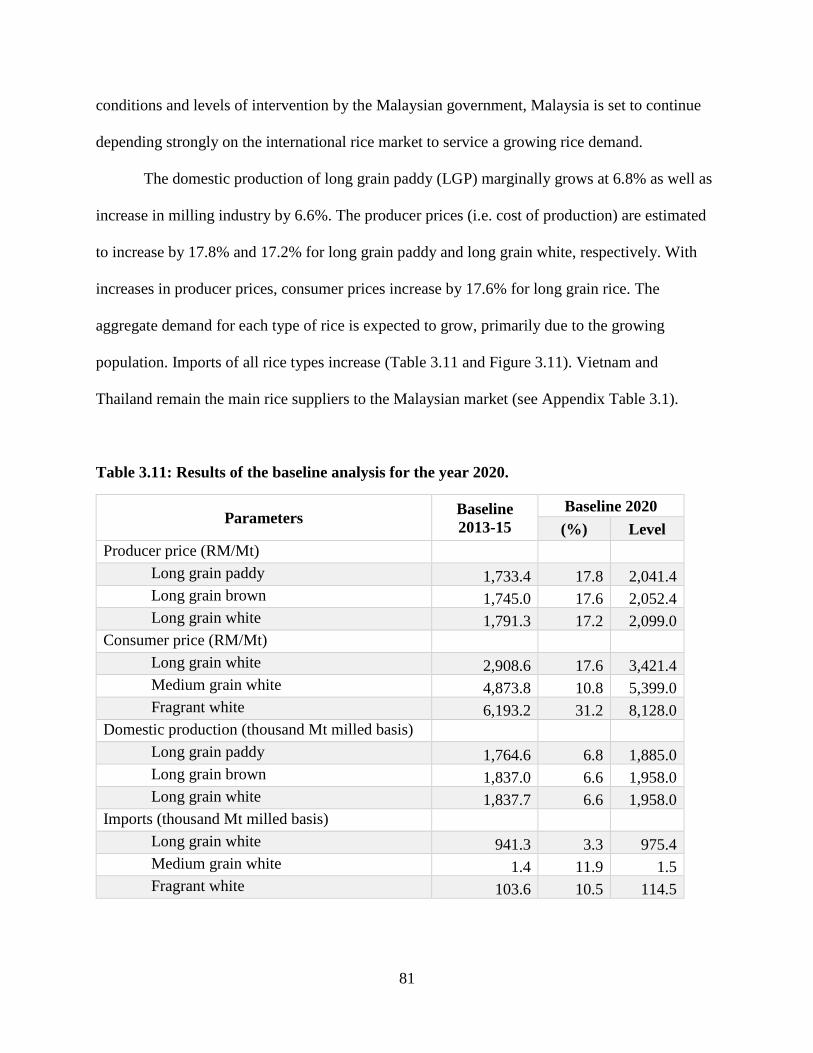
81
conditions and levels of intervention by the Malaysian government, Malaysia is set to continue
depending strongly on the international rice market to service a growing rice demand.
The domestic production of long grain paddy (LGP) marginally grows at 6.8% as well as
increase in milling industry by 6.6%. The producer prices (i.e. cost of production) are estimated
to increase by 17.8% and 17.2% for long grain paddy and long grain white, respectively. With
increases in producer prices, consumer prices increase by 17.6% for long grain rice. The
aggregate demand for each type of rice is expected to grow, primarily due to the growing
population. Imports of all rice types increase (Table 3.11 and Figure 3.11). Vietnam and
Thailand remain the main rice suppliers to the Malaysian market (see Appendix Table 3.1).
Table 3.11: Results of the baseline analysis for the year 2020.
Parameters Baseline
2013-15
Baseline 2020
(%) Level
Producer price (RM/Mt)
Long grain paddy 1,733.4 17.8 2,041.4
Long grain brown 1,745.0 17.6 2,052.4
Long grain white 1,791.3 17.2 2,099.0
Consumer price (RM/Mt) Long grain white 2,908.6 17.6 3,421.4
Medium grain white 4,873.8 10.8 5,399.0
Fragrant white 6,193.2 31.2 8,128.0
Domestic production (thousand Mt milled basis) Long grain paddy 1,764.6 6.8 1,885.0
Long grain brown 1,837.0 6.6 1,958.0
Long grain white 1,837.7 6.6 1,958.0
Imports (thousand Mt milled basis) Long grain white 941.3 3.3 975.4
Medium grain white 1.4 11.9 1.5
Fragrant white 103.6 10.5 114.5

82
Table 3.11 (Cont.)
Parameters Baseline
2013-15
Baseline 2020
% Level
Demand (thousand Mt milled basis)
Long grain white 2,779.0 5.5 2,932.0
Medium grain white 1.4 11.6 1.5
Fragrant white 103.7 10.7 114.8
Self-sufficiency level in long grain (%) 66.1 66.7
These results suggest that Malaysia’s goal of achieving rice self-sufficiency by 2020 are
unrealistic at the projected market and government intervention conditions.
Figure 3.11: Projections on Malaysia’s rice imports by 2020.
4.2 Self-sufficiency Scenario
The results of the self-sufficiency scenario for rice commodities in Malaysia are
presented in Table 3.12. Recall that this scenario entails reducing imports of long grain rice by
95%. The massive decrease in rice imports stimulate the domestic production to increase by
Long Grain,
90.2%
Fragrant Rice
9.6%
Medium Grain
0.1%

83
53.3%, which is only possible with a 170.3% increase in producer price. By the underlying a
zero-profit condition21, this increase also implies the increase in cost of production that is mostly
derived from a constraint in land factor. The higher production cost of paddy rice and
consequential increase in the market price of paddy rice transfers to higher consumer prices. As
a result, the demand for long grain rice declines by 23.9%.
Rice producers gain as a result of the self-sufficiency policy due to increases in producer
surplus. However, rice consumers are worse off since the market prices are much higher (i.e.
decrease in consumer surplus), hence rice self-sufficiency entails significant welfare shifts from
consumers to producers. These results suggest that self-sufficiency will likely adversely affect
food security objectives since the policy increases prices and limits consumption.
Table 3.12: Results of the self-sufficiency scenario.
Parameters Baseline
2013-15
Baseline 2020 Self-sufficiency
(%) Level (%) Level
Producer price (RM/Mt)
Long grain paddy 1,733.4 17.8 2,041.4 170.3 5,516.9
Long grain brown 1,745.0 17.6 2,052.4 168.9 5,519.3
Long grain white 1,791.3 17.2 2,099.0 165.3 5,567.6
Consumer price (RM/Mt)
Long grain white 2,908.6 17.6 3,421.4 165.3 9,075.3
Medium grain white 4,873.8 10.8 5,399.0 0.0 5,399.0
Fragrant white 6,193.2 31.2 8,128.0 0.2 8,146.7
Domestic production (thousand Mt) Long grain paddy 1,764.6 6.8 1,885.0 53.3 2,890.5
Long grain brown 1,837.0 6.6 1,958.0 51.4 2,965.0
Long grain white 1,837.7 6.6 1,958.0 51.2 2,959.9
Imports (thousand Mt milled basis) Long grain white 9,41.3 3.3 975.4 -95.0 48.8
Medium grain white 1.4 11.9 1.5 7.1 1.6
Fragrant white 103.6 10.5 114.5 7.1 122.6
21 By virtue of the zero-profit condition, the product price by activity equals the unitary cost of
production (Durand-Morat and Wailes, 2010).
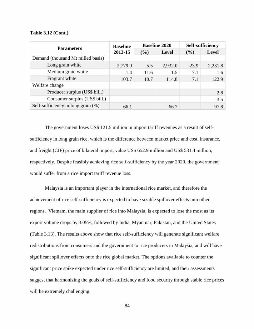
84
Table 3.12 (Cont.)
Parameters Baseline
2013-15
Baseline 2020 Self-sufficiency
(%) Level (%) Level
Demand (thousand Mt milled basis) Long grain white 2,779.0 5.5 2,932.0 -23.9 2,231.8
Medium grain white 1.4 11.6 1.5 7.1 1.6
Fragrant white 103.7 10.7 114.8 7.1 122.9
Welfare change
Producer surplus (US$ bill.) 2.8
Consumer surplus (US$ bill.) -3.5
Self-sufficiency in long grain (%) 66.1 66.7 97.8
The government loses US$ 121.5 million in import tariff revenues as a result of self-
sufficiency in long grain rice, which is the difference between market price and cost, insurance,
and freight (CIF) price of bilateral import, value US$ 652.9 million and US$ 531.4 million,
respectively. Despite feasibly achieving rice self-sufficiency by the year 2020, the government
would suffer from a rice import tariff revenue loss.
Malaysia is an important player in the international rice market, and therefore the
achievement of rice self-sufficiency is expected to have sizable spillover effects into other
regions. Vietnam, the main supplier of rice into Malaysia, is expected to lose the most as its
export volume drops by 3.05%, followed by India, Myanmar, Pakistan, and the United States
(Table 3.13). The results above show that rice self-sufficiency will generate significant welfare
redistributions from consumers and the government to rice producers in Malaysia, and will have
significant spillover effects onto the rice global market. The options available to counter the
significant price spike expected under rice self-sufficiency are limited, and their assessments
suggest that harmonizing the goals of self-sufficiency and food security through stable rice prices
will be extremely challenging.

85
Table 3.13: Global impacts of self-sufficiency policy in Malaysia.
Exporting Regions % Change of Export Volume
Vietnam -3.05
Thailand -0.14
Pakistan -1.54
Myanmar -1.63
India -1.70
United States -1.53
ROW (Rest of the World) -1.83
4.3 Output Subsidy Requirements
An option to offset the rice price increase resulting from rice self-sufficiency could be to
expand producer subsidies. The subsidy expansion would bring the consumer price down at the
pre-self-sufficiency level, so the price becomes lower. The required subsidy and the cost of the
subsidy program can be estimated using the producer prices and domestic production in the self-
sufficiency scenario. The total subsidy (in local currency per metric ton) is estimated at RM
3,475.5/Mt (US$ 810/Mt). The total cost of subsidy program is estimated at RM 10.04 billion
(US$ 2.34 billion). With the current total subsidy program is RM 1.8 billion (DOA, 2010), the
government needs a substantial additional expenditure to realize self-sufficiency in rice while
maintaining prices at the baseline level (Table 3.14).
Table 3.14: Required subsidy and total subsidy program for self-sufficiency.
Parameter Producer Prices (RM/Mt)
RM/ Mt Baseline 2020 Self-sufficiency
Required subsidy
2,041.4
5,516.9
3,475.5
Total subsidy
(RM/Mt)
Domestic production (thousand
Mt in paddy basis) RM (Billion)
Required total subsidy
3,475.5
2,890.5
10.04

86
4.4 The Requirements of Production Input.
The primary rice production technology is specified as Leontief production function (no
substitution between production inputs). Additionally, all factors of production are assumed to be
perfectly elastically supplied except for land. This specification of production and input markets
means that the changes in the rice market will be primarily dictated by the specification of land
markets. In the self-sufficiency scenario, the growth of domestic production (53.3%) translates
into a 53.3% increase in land demand. Given the inelastic supply of land assumed in this study,
such an expansion in land demand results in very large increases in land rental rates (Table 3.15).
The increase in required land in the self-sufficiency scenario would also lead to an incredibly
higher cost of production, subsequently would transfer to much higher consumer prices.
Table 3.15: The required land input of production.
Parameters Baseline 2020 Self-sufficiency
Rice acreage at baseline (‘000 Ha) 690.0 736.9
Growth in required land input (%) 6.8 53.3
Required land acreage (‘000 Ha) 736.9 1,129.8
Domestic rice production (‘000 Mt, paddy basis) 1,885 2,890.5
The majority of agricultural land in Malaysia is used to produce palm oil and rubber,
which the most important agricultural commodities for the national income, thus rice farmland is
limited to less than 10% of the total agricultural land (Figure 3.12). The land substitution
possibilities between an annual crop such as rice and permanent crops such as rubber and palm
oil are limited by the high investment required in the later.

87
Source: FAOSTAT (2014)
Figure 3.12: Malaysia: Agricultural land use (area harvested) by commodity.
Possible solutions to overcome the land constraint include the utilization of technology
and research and development such as the development of non-irrigated farmland, but it is still
challenging for Malaysia regarding land availability. To expand rice acreage, another way is
through increasing rice-land-use intensity (number of rice crops produced per year on the same
field). However, the existing crop intensity in Malaysia is relatively high, ranging from 170% to
180%. Forcing the crop intensity to be much higher would be extremely challenging, especially
with respect to the agronomy dimensions and crucial water resource adequacy (FAO, 2005).
4.5 The Requirement for Technological Efficiency.
Technological efficiency is based on the intensification of productivity, primarily land
productivity. Higher yields per hectare can enable Malaysia to achieve higher output without
increasing acreage. Therefore, the required crop yield to achieve self-sufficiency, which
represents the needed productivity improvement, is measured. At the baseline 2020, with the
land acreage of 690 (thousand ha) to produce 1,958 (thousand Mt, milled basis), the required
67.85%
15.42%
9.98%
6.75%
0% 10% 20% 30% 40% 50% 60% 70% 80%
Oil palm
Rubber
Rice
Others

88
crop yield is 2.83 Mt/ha22 (milled basis) or 4.73 Mt/ha (paddy basis). In self-sufficiency scenario,
with the required land acreage is 736.9 (thousand ha) to produce 2,959.9 (thousand Mt, milled
basis) rice, the required crop yield is 4.02 Mt/ha (milled basis) or 6.18 Mt/ha (paddy basis). At
this productivity gain, domestic rice production can be achieved at the self-sufficiency level and
consumer prices remain at the pre-self-sufficiency level, thus preventing prices from surging up
(Table 3.16). However, these findings suggest that the challenge for Malaysia to achieve self-
sufficiency while keeping rice price stability is significant and would require yield gains of 30%
in relatively few years. To put this in perspective, it took Malaysia around 15 years (since 1998-
2000) to increase average rice yields by 30 percent to reach the 2014-16 average yield of 4.02
Mt/ha (paddy basis).
Table 3.16: The required technological efficiency on productivity.
Parameters Baseline 2020 Self-sufficiency
Land acreage (in thousand ha) 690.0 736.9
Domestic production (in thousands, milled basis) 1,958.0 2,959.9
Required crop yield Mt/ha (in milled basis) 2.83 4.02
Required crop yield Mt/ha (in paddy basis) 4.73 6.18
Since most of the tropical rice-growing countries in Asia have a high population growth
rate and limited land for rice cultivation, in order to be a food-secured nation, the productivity
gain is crucial. Hybrid rice adoption can be a way to meet this objective (FAO, 2004). The
hybrid rice technology aims to increase the yield potential of rice beyond the level of inbred
high-yielding varieties (HYVs) by exploiting the phenomenon of hybrid vigor or heterosis.
22 The crop yield is estimated as the division of domestic production (1,885 in thousand Mt,
paddy basis) to the land acreage (736.9 in thousand ha).

89
However, a number of challenges have been identified which affect the large-scale adoption of
hybrid rice, including inferior grain quality, and the high cost of seed (FAO, 2004). Another
potential technology for limited irrigated land is the upland rice, which are grown in well-
drained, non-puddled, and non-saturated soils. With good management practices, upland rice
(aerobic rice) tends to produce at least 4-6 Mt/ha, however more species of weeds tend
to experience in rice field that are not permanently flooded than in flooded rice, especially in the
tropic environments. Also, soil-borne pests and diseases such as nematodes, root aphids, and
fungi have been found to possibly occur more in upland rice (Maclean et al., 2013). Malaysia has
ventured in both hybrid and upland rice varieties through the Malaysian Agricultural Research
and Development Institute (MARDI) since 2005. Since the hybrid rice does not perform well
with a direct-seeding approach, which the most applied planting approach in Malaysia, farmers
need to apply a high-technology machinery for planting process, which is not available to most
small rice farmers. As a result, “Earlier works on hybrid rice in Malaysia had never delivered a
success” (GRAIN, 2008). Aerobic rice, a combination of upland and high-yield lowland rice
varieties (Tuong and Bouman, 2003) is another effort to achieve self-sufficiency in rice. Despite
having been stable productivity, the aerobic rice resulted in lower crop yields than irrigated
lowland rice, ranged 2.2 to 3.6 Mt/ha. In fact, the aerobic rice tends to expose higher weed
infestation with a poor soil structure in adverse non-irrigated environment, which was
consistently required higher inputs. With most rice farmers in Malaysia are among the poor, this
condition would be the most challenging to maintain the production performance (Chan et al.,
2012).

90
4.6 Free Trade Scenario
As described above, the free-trade scenario implies removing all existing long grain rice
import tariffs in Malaysia (see Appendix Table 3.3 for information on the actual levels of import
protection administered by Malaysia). With free trade, the producer price for long grain rice in
Malaysia decreases by 11.9%, and domestic production by 5.3%, yielding a self-sufficiency level
of 61.8%. The increased competition in the Malaysian rice market leads to a reduction in
consumer prices of 14.74% and a consequent increase in domestic consumption of long grain
rice of 4.44%. The higher domestic demand further expands rice imports by 19.85% (Table
3.17).
The results are consistent with the trade theory that reveals rice producers lose, yet
consumers gain and better off from the international free trade policy. From the consumers’
perspectives, a free trade scenario appears to allow for a more food secured economy relative to
a self-sufficiency scenario, since the free trade is not punishing consumers at the price level and
thus, consumers gain from the free trade. However, producers would be worse off (i.e. decrease
producer surplus), and the government will lose tariff revenues from the free trade.
Table 3.17: Results of free trade scenario.
Parameters Baseline
2013-15
Baseline 2020 Free Trade Policy
(%) Level (%) Level
Producer price (RM/Mt)
Long grain paddy 1,733.40 17.80 2,041.40 -11.90 1,798.47
Long grain brown 1,744.90 17.60 2,052.40 -11.81 1,810.01
Long grain white 1,791.30 17.20 2,099.00 -11.55 1,856.57
Consumer price (RM/Mt)
Long grain white 2,908.60 17.60 3,421.40 -14.74 2,917.09
Medium grain white 4,874.00 10.80 5,399.00 0.01 5,399.54
Fragrant white 6,193.00 31.20 8,128.00 -0.04 8,124.75

91
Table 3.17 (Cont.)
Parameters Baseline
2013-15
Baseline 2020 Free Trade
(%) Level (%) Level
Domestic production
(thousand Mt) Long grain paddy 1,764.60 6.80 1,885 -5.30 1,785.10
Long grain brown 1,837.00 6.60 1,958 -5.11 1,857.95
Long grain white 1,837.70 6.60 1,958 -5.08 1,858.53
Imports (thousand Mt
milled basis) Long grain white 941.3 3.30 975.4 19.85 1,169.02
Medium grain white 1.4 11.90 1.5 -1.08 1.48
Fragrant white 103.6 10.50 114.5 -1.08 113.26
Demand (thousand Mt
milled basis) Long grain white 2,779.00 5.50 2,932.00 4.44 3,062.18
Medium grain white 1.4 11.60 1.5 -1.08 1.48
Fragrant white 103.7 10.70 114.8 -1.08 113.56
Welfare change
Producer surplus
(US$ mill.) -125.8
Consumer surplus
(US$ mill.) 328.0
Self-sufficiency level (%) 66.13 66.73 61.82
While self-sufficiency policy would improve welfare to rice producers, albeit a minor
segment of total population, the policy will not only lead to a substantial increase in consumer
prices, but also gargantuan government costs. Instead, free trade could be welfare improving to
most of the population of the country as rice remains a primary food staple. From a policy
perspective, the government and policymakers should gauge the implications of the policies on
economy as a whole. The government’s stance on self-sufficiency needs to be reconsidered as
this policy strategy is economically misguided. The significant differences in welfare allocation
between the two scenarios described above imply that the political economy becomes even more
crucial in deciding the policy output. Since Malaysia is pursuing self-sufficiency, the forces

92
supporting a small group of the population are winning the battle to the expense of the larger
consumer group.
5. Conclusions
Rice self-sufficiency has become a policy cornerstone in Malaysia, and it is a maintained
strategy to be the best way to address food security concerns. Various strategies can be utilized
to achieve a desired level of self-sufficiency which lead to substantial public investment to
support domestic rice production. As a result, rice has become a highly subsidized and protected
food crop. The government’s mandate is to seriously pursue self-sufficiency in rice and achieve
the policy goal by the years 2020.Most recently this goal has been extended to 2050. With this
mandate, the government aims to close all trading borders and eliminate rice imports coming
from international markets and suppliers. As Malaysia is not a competitive rice producer, this
extreme policy decision will require a massive additional expenditure at the production level.
Instead, liberalizing rice trade offers positive effects on food security and implicitly economic
growth as Malaysia has actively participated in both bilateral and regional free trade agreements.
This study evaluates and analyzes the impact of self-sufficiency and free trade policies on
rice sector in Malaysia at the national level using a spatial partial equilibrium model. As
expected, the results correspond to economic theory with self-sufficiency greatly benefitting rice
farmers at the expense of consumers. On the other hand, the free trade showed opposite policy
impact since farmers’ welfare will be worsen while increasing consumers’ welfare. From this
study, these two policy scenarios clearly represent the opposite direction in terms of welfare
distribution, and the estimations of producer and consumer surplus corroborate the findings. Self-
sufficiency will create massive welfare shifts from consumers and the government to rice

93
producers. Despite improving welfare to rice producers, albeit a small group, self-sufficiency
punish consumers, which also include rice producers, due to highly increased consumer price. As
affordable food price is a key concepts of food security, self-sufficiency does not guarantee food
security at the national level. The government loses from self-sufficiency, thus pursuing self-
sufficiency is highly challenging for Malaysia. As part of the ASEAN, Malaysia could
participate in a regional approach for strengthening food security to address its rice-deficit issue.
Instead, free trade offers a more food secured economy. With free trade, although rice producers
are worse off, albeit a marginal degree, and the government loses from import tariff revenues, the
consumers would be better off due to decreasing prices with a more competitive market
environment from external rice suppliers.
Since this study focuses on rice in terms of final consumption, the model is not allowed
for substitution to other sources of calories which means consumers continue to consume rice
with no substitutions. As dictated by elasticities, consumers are not allowed to switch to wheat,
corn, and etc. Further analysis should focus on substitution of other food sources in the final
consumption. Also, the estimations for each parameter are based on the fact that Malaysia
pursues total self-sufficiency goal by the year 2020, as mandated by the government in the
national agricultural policy for 2010-2020. However, the government has recently extended the
self-sufficiency goal to the year 2050 under the national masterplan for 2020 - 2050, and thus the
country has another 30 years to improve its rice sector to achieve self-sufficiency in the future.

94
References
Armington, P. A. 1969. A theory of demand for products distinguished by place of production.
IMF Staff Papers 16: 159-178.
Chan, C.S., Zainudin, H., Saad, A., and Azmi, M. 2012. Productive Water Use in Aerobic Rice
Cultivation. J. Trop. Agric. and Food Sc. 49:1, pp 117– 126.
Clapp, J. 2017. Food self-sufficiency: Making sense of it, and when it makes sense. Food Policy
66 (2017) 88 – 96.
Clapp, J. 2014. Food Security and Food Sovereignty: Getting Past the Binary. Dialogues Human
Geogr. 4 (2), 106–211.
Daviron, B, Dembele, N, Murphy, S, and Rashid, S. Price Volatility and Food Security. A Report
by the High Level of Experts on Food Security and Nutrition of the Committee on World
Food Security.
Department of Agriculture, Malaysia (DOA). 2010. Subsidy and Agricultural Incentives for
Farmers. www.pmr.penerangan.gov.my.
Durand-Morat, A and Wailes, E. 2010. A Multi-Region, Multi-Project, Spatial Partial
Equilibrium Model of the World Rice Economy.
FAO - Food and Agriculture Organization. 2016. Food Self-Sufficiency and International Trade:
A False Dichotomy? The State of Agricultural Commodity Markets in Depth.
FAO - Food and Agriculture Organization. 2011. The State of the World’s Land and Water
Resources for Food and Agriculture: Managing Systems at Risk. United Nation.
FAO - Food and Agriculture Organization. 2010. Challenges for a Wealthier World: Meat for
All?
FAO - Food and Agriculture Organization. 2008. An Introduction to the Basic Concepts of Food
Security.
95
FAO - Food and Agriculture Organization. 2004. Hybrid Rice for Food Security. United Nation.
FAO - Food and Agriculture Organization.1999. Implications of Economic Policy for Food
Security: A Training Manual.
GRAIN. 2008. Malaysia: Hybrid Rice and the Decline in Public Breeding.
IFPRI – International Food Policy Research Institute. 2014. Global Nutrition Report.
Jolly, C.M., Bayard, B., and Nguyen, G. 2009. Investigating Food Self-Sufficiency Challenges in
Haiti.
Mailena, L., Shamsudin, M.N., Radam, A., and Latief, I. 2014. Rice Farms Efficiency and
Factors Affecting the Efficiency in MADA Malaysia. Journal of Applied Science, Vol.
14: 18, pp. 2177 – 2182. DOI: 10.3923/jas.2014.2177.2182.
Maclean, J., Hardy, B., and Hettel, G. 2013. Rice Almanac. CGIAR.
Mankiw, G. 2009. Principles of Macroeconomics, Fifth Edition.
MOA - Ministry of Agriculture and Agro-Based Industry. 2011-2014. National Agro-Food
Policy 2011-2020. Division of International and Strategic Planning. Putrajaya, Malaysia,
ISBN: 978-983-9863-41-3.
MITI - Malaysian International and Trade Industry. 2006. Malaysian International and Trade
Industry Report.
Mosavi, S, H, and Esmaeili, A. 2012. Self-Sufficiency versus Free Trade: The Case of Rice in
Iran. Journal of International Food and Agribusiness Marketing, Vol. 24:1.
Naylor, R, L. and Falcon, W, P. 2010. Food Security in an Era of Economic Volatility.
Population and Development Review.
OECD. 2008. Making Trade Works for Developing Countries. Policy Brief.
96
Panagariya, A. 2002. Costs, benefits and risks from trade: theory and practice for food
security presented at the FAO Expert Consultation on Trade and Food Security:
Conceptualizing the Linkages. Rome, 11-12 July 2002.
Rodrik, D. 2007. One economics, Many Recipes: Globalization, Institutions, and Economic
Growth.
Rosegrant, M. W, Paisner, M.S, Meijer, S, and Witcover, J. 2001. 2020 Global Food Outlook.
Washington, DC: International Food Policy Research Institute.
Stockman, A.C. 1999. Introduction to Economics, Second Edition.
Tuong, T.P., and Bouman, B.A.M. 2003. Rice production in water scarce environment. In: Water
productivity in agriculture: Limits and opportunities for improvement. (Kijne, J.W. and
Molden, D.), pp. 53–67. Wallingford (UK): CABI Publishing
Von Braun, J. and Diaz-Bonilla, E. 2008. Globalization of Food and Agriculture and the Poor.
Oxford University Press.
Von Braun, J. and Paulino, L. 1990. Food in Sub-Saharan Africa: Trends and Policy Challenges
for the 1990s. Food Policy, 15(6), pp. 505-517.
Wailes, E. and Chavez, E. 2011. Updated Arkansas Global Rice Model. Department of
Agricultural Economics and Agribusiness, Division of Agriculture, University of
Arkansas, Fayetteville, United States.
Wailes, E, Durand-Morat, A, Hoffman, L, and Childs, N. 2004. Tariff Escalation: Impacts on
U.S. and Global Rice Trade. American Agricultural Economics Association Annual
Meeting, Denver Colorado, August 1-4, 2004.
World Bank. 2012. Global Monitoring Report 2012: Food Prices, Nutrition, and the Millennium
Development Goals. World Bank, Washington, D.C.
World Bank. 2002. Globalization, Growth, and Poverty: Building an Inclusive World Economy.
Washington D.C: World Bank.
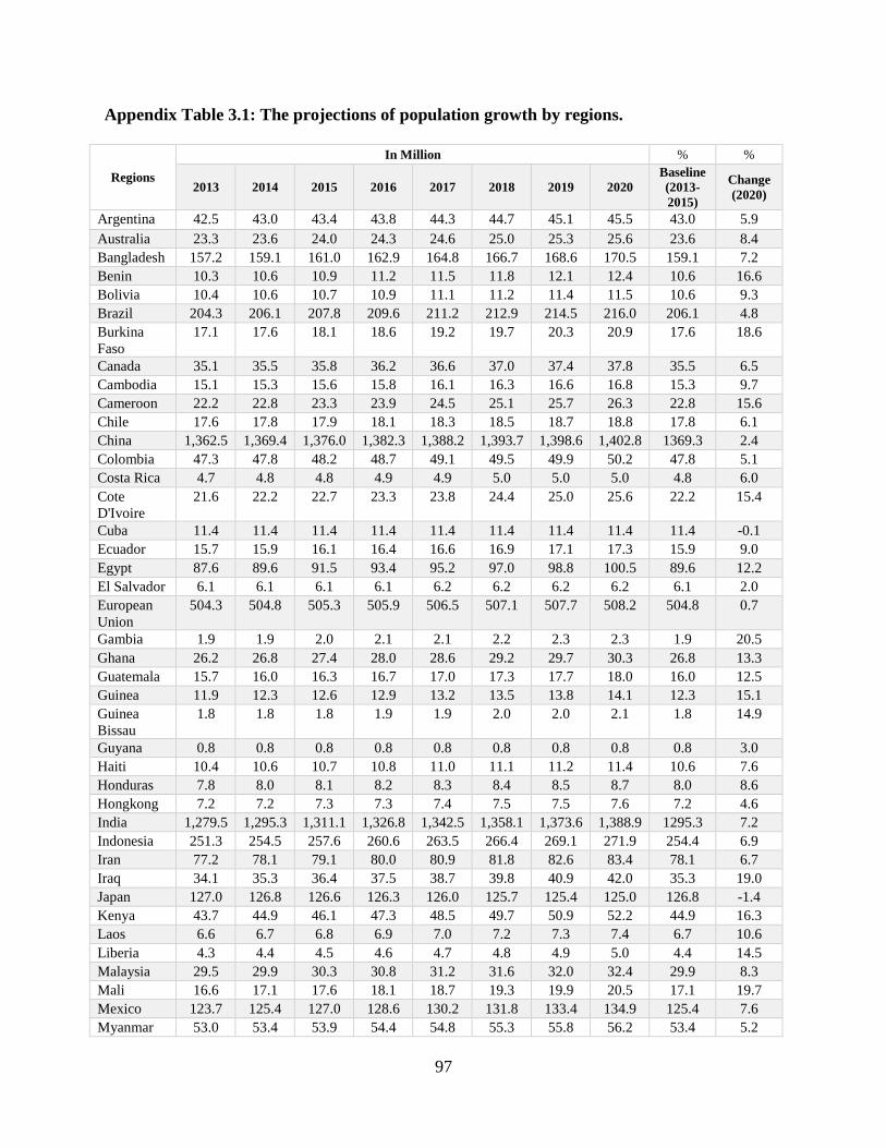
97
Appendix Table 3.1: The projections of population growth by regions.
Regions
In Million % %
2013 2014 2015 2016 2017 2018 2019 2020
Baseline
(2013-
2015)
Change
(2020)
Argentina 42.5 43.0 43.4 43.8 44.3 44.7 45.1 45.5 43.0 5.9
Australia 23.3 23.6 24.0 24.3 24.6 25.0 25.3 25.6 23.6 8.4
Bangladesh 157.2 159.1 161.0 162.9 164.8 166.7 168.6 170.5 159.1 7.2
Benin 10.3 10.6 10.9 11.2 11.5 11.8 12.1 12.4 10.6 16.6
Bolivia 10.4 10.6 10.7 10.9 11.1 11.2 11.4 11.5 10.6 9.3
Brazil 204.3 206.1 207.8 209.6 211.2 212.9 214.5 216.0 206.1 4.8
Burkina
Faso
17.1 17.6 18.1 18.6 19.2 19.7 20.3 20.9 17.6 18.6
Canada 35.1 35.5 35.8 36.2 36.6 37.0 37.4 37.8 35.5 6.5
Cambodia 15.1 15.3 15.6 15.8 16.1 16.3 16.6 16.8 15.3 9.7
Cameroon 22.2 22.8 23.3 23.9 24.5 25.1 25.7 26.3 22.8 15.6
Chile 17.6 17.8 17.9 18.1 18.3 18.5 18.7 18.8 17.8 6.1
China 1,362.5 1,369.4 1,376.0 1,382.3 1,388.2 1,393.7 1,398.6 1,402.8 1369.3 2.4
Colombia 47.3 47.8 48.2 48.7 49.1 49.5 49.9 50.2 47.8 5.1
Costa Rica 4.7 4.8 4.8 4.9 4.9 5.0 5.0 5.0 4.8 6.0
Cote
D'Ivoire
21.6 22.2 22.7 23.3 23.8 24.4 25.0 25.6 22.2 15.4
Cuba 11.4 11.4 11.4 11.4 11.4 11.4 11.4 11.4 11.4 -0.1
Ecuador 15.7 15.9 16.1 16.4 16.6 16.9 17.1 17.3 15.9 9.0
Egypt 87.6 89.6 91.5 93.4 95.2 97.0 98.8 100.5 89.6 12.2
El Salvador 6.1 6.1 6.1 6.1 6.2 6.2 6.2 6.2 6.1 2.0
European
Union
504.3 504.8 505.3 505.9 506.5 507.1 507.7 508.2 504.8 0.7
Gambia 1.9 1.9 2.0 2.1 2.1 2.2 2.3 2.3 1.9 20.5
Ghana 26.2 26.8 27.4 28.0 28.6 29.2 29.7 30.3 26.8 13.3
Guatemala 15.7 16.0 16.3 16.7 17.0 17.3 17.7 18.0 16.0 12.5
Guinea 11.9 12.3 12.6 12.9 13.2 13.5 13.8 14.1 12.3 15.1
Guinea
Bissau
1.8 1.8 1.8 1.9 1.9 2.0 2.0 2.1 1.8 14.9
Guyana 0.8 0.8 0.8 0.8 0.8 0.8 0.8 0.8 0.8 3.0
Haiti 10.4 10.6 10.7 10.8 11.0 11.1 11.2 11.4 10.6 7.6
Honduras 7.8 8.0 8.1 8.2 8.3 8.4 8.5 8.7 8.0 8.6
Hongkong 7.2 7.2 7.3 7.3 7.4 7.5 7.5 7.6 7.2 4.6
India 1,279.5 1,295.3 1,311.1 1,326.8 1,342.5 1,358.1 1,373.6 1,388.9 1295.3 7.2
Indonesia 251.3 254.5 257.6 260.6 263.5 266.4 269.1 271.9 254.4 6.9
Iran 77.2 78.1 79.1 80.0 80.9 81.8 82.6 83.4 78.1 6.7
Iraq 34.1 35.3 36.4 37.5 38.7 39.8 40.9 42.0 35.3 19.0
Japan 127.0 126.8 126.6 126.3 126.0 125.7 125.4 125.0 126.8 -1.4
Kenya 43.7 44.9 46.1 47.3 48.5 49.7 50.9 52.2 44.9 16.3
Laos 6.6 6.7 6.8 6.9 7.0 7.2 7.3 7.4 6.7 10.6
Liberia 4.3 4.4 4.5 4.6 4.7 4.8 4.9 5.0 4.4 14.5
Malaysia 29.5 29.9 30.3 30.8 31.2 31.6 32.0 32.4 29.9 8.3
Mali 16.6 17.1 17.6 18.1 18.7 19.3 19.9 20.5 17.1 19.7
Mexico 123.7 125.4 127.0 128.6 130.2 131.8 133.4 134.9 125.4 7.6
Myanmar 53.0 53.4 53.9 54.4 54.8 55.3 55.8 56.2 53.4 5.2

98
Appendix Table 3.1 (Cont.)
Regions
In Million % %
2013 2014 2015 2016 2017 2018 2019 2020
Baseline
(2013-
2015)
Change
(2020)
Nicaragua 5.9 6.0 6.1 6.2 6.2 6.3 6.4 6.4 6.0 6.7
Niger 18.4 19.1 19.9 20.7 21.6 22.4 23.4 24.3 19.1 27.1
Nigeria 172.8 177.5 182.2 187.0 191.8 196.8 201.7 206.8 177.5 16.5
Pakistan 181.2 185.0 188.9 192.8 196.7 200.7 204.6 208.4 185.1 12.6
Panama 3.8 3.9 3.9 4.0 4.1 4.1 4.2 4.2 3.9 9.4
Paraguay 6.5 6.6 6.6 6.7 6.8 6.9 7.0 7.1 6.6 7.9
Peru 30.6 31.0 31.4 31.8 32.2 32.6 32.9 33.3 31.0 7.6
Philippines 97.6 99.1 100.7 102.3 103.8 105.3 106.9 108.4 99.1 9.4
Rwanda 11.1 11.3 11.6 11.9 12.2 12.4 12.7 13.0 11.3 14.6
Russia 143.4 143.4 143.5 143.4 143.4 143.3 143.1 142.9 143.4 -0.4
Saudi
Arabia
30.2 30.9 31.5 32.2 32.7 33.3 33.8 34.4 30.9 11.3
Senegal 14.2 14.7 15.1 15.6 16.1 16.5 17.0 17.5 14.7 19.2
Singapore 5.4 5.5 5.6 5.7 5.8 5.9 5.9 6.0 5.5 9.1
Sierra
Leone
6.2 6.3 6.5 6.6 6.7 6.9 7.0 7.2 6.3 13.6
South
Korea
49.8 50.1 50.3 50.5 50.7 50.9 51.1 51.3 50.1 2.4
South
Africa
53.4 54.0 54.5 55.0 55.4 55.9 56.3 56.7 54.0 5.0
Sri Lanka 20.5 20.6 20.7 20.8 20.9 21.0 21.1 21.2 20.6 2.6
Suriname 0.5 0.5 0.5 0.5 0.6 0.6 0.6 0.6 0.5 5.0
Taiwan 23.3 23.4 23.5 23.5 23.6 23.6 23.7 23.7 23.4 1.4
Tanzania 50.2 51.8 53.5 55.2 56.9 58.6 60.4 62.3 51.8 20.1
Thailand 67.5 67.7 68.0 68.1 68.3 68.4 68.5 68.6 67.7 1.3
Togo 6.9 7.1 7.3 7.5 7.7 7.9 8.1 8.3 7.1 16.5
Turkey 76.2 77.5 78.7 79.6 80.4 81.1 81.7 82.3 77.5 6.2
UAE 9.0 9.1 9.2 9.3 9.4 9.5 9.7 9.8 9.1 8.0
Uganda 36.6 37.8 39.0 40.3 41.7 43.0 44.4 45.9 37.8 21.3
Uruguay 3.4 3.4 3.4 3.4 3.5 3.5 3.5 3.5 3.4 2.2
USA 317.1 319.5 322.0 324.5 327.1 329.8 332.4 335.0 319.5 4.8
Venezuela 30.3 30.7 31.1 31.5 31.9 32.3 32.7 33.1 30.7 7.9
Vietnam 91.4 92.4 93.4 94.4 95.4 96.4 97.3 98.2 92.4 6.2
Source: Arkansas Global Rice Model (AGRM).

99
Appendix Table 3.2: The projections of gross domestic product by regions.
Regions
Billion US$ % %
2013 2014 2015 2016 2017 2018 2019 2020
Baseline
(2013-
2015)
Change
2020
Argentina 458.1 446.7 457.5 450.0 476.3 476.3 489.9 502.0 454.1 10.6
Australia 1357.4 1395.3 1428.9 1463.4 1537.7 1537.7 1583.1 1627.3 1393.8 16.7
Bangladesh 137.7 146.0 155.6 166.5 188.6 188.6 200.9 213.7 146.4 45.9
Benin 7.5 8.0 8.3 8.7 9.4 9.4 9.8 10.2 7.9 28.6
Bolivia 23.2 24.5 25.7 26.6 28.6 28.6 29.8 31.1 24.4 27.2
Brazil 2412.8 2424.9 2333.4 2250.5 2307.1 2307.1 2385.4 2475.5 2390.3 3.6
Burkina Faso 10.8 11.4 11.9 12.4 13.8 13.8 14.5 15.3 11.4 34.6
Canada 1735.2 1779.7 1796.5 1820.2 1901.6 1901.6 1945.0 1984.2 1770.4 12.1
Cambodia 13.9 14.8 15.9 17.0 19.4 19.4 20.7 22.0 14.9 48.3
Cameroon 27.2 28.8 30.1 31.6 34.9 34.9 36.6 38.3 28.7 33.4
Chile 253.1 257.7 263.6 267.6 279.6 279.6 288.7 300.2 258.1 16.3
China 7748.4 8314.0 8889.9 9485.2 10717.2 10717.2 11370.2 12062.3 8317.4 45.0
Colombia 334.2 348.9 359.6 366.8 383.8 383.8 394.7 407.6 347.6 17.3
Costa Rica 41.6 42.8 44.4 46.1 49.6 49.6 51.6 53.7 42.9 25.1
Cote D'Ivoire 28.8 31.2 33.7 36.3 41.5 41.5 43.5 45.3 31.2 45.0
Cuba 70.0 70.7 73.8 74.3 78.9 78.9 82.3 86.2 71.5 20.6
Ecuador 83.2 86.5 86.6 84.5 87.0 87.0 89.4 91.9 85.4 7.5
Egypt 228.0 233.1 242.9 253.6 277.3 277.3 290.9 305.3 234.7 30.1
El Salvador 22.7 23.0 23.6 24.1 25.1 25.1 25.6 26.2 23.1 13.1
European
Union
17240.3 17521.1 17895.8 18226.8 18506.3 18812.2 19110.3 19406.4 17552.4 10.6
Gambia 1.0 1.0 1.1 1.1 1.2 1.2 1.2 1.3 1.0 25.8
Ghana 43.0 44.8 46.5 48.1 54.4 54.4 57.7 60.5 44.8 35.1
Guatemala 46.0 47.9 49.9 51.6 55.1 55.1 57.1 59.2 47.9 23.6
Guinea 5.2 5.3 5.3 5.5 6.0 6.0 6.4 6.8 5.3 29.1
Guinea
Bissau
0.9 0.9 1.0 1.0 1.1 1.1 1.2 1.2 0.9 28.6
Guyana 2.3 2.4 2.4 2.5 2.7 2.7 2.8 2.9 2.4 23.9
Haiti 7.6 7.8 7.9 8.0 8.3 8.3 8.5 8.7 7.8 12.5
Honduras 17.6 18.1 18.8 19.5 20.8 20.8 21.6 22.4 18.2 23.2
Hong Kong 252.0 258.3 264.7 268.8 278.7 278.7 284.7 291.4 258.3 12.8
India 1895.6 2032.1 2185.5 2336.9 2702.8 2702.8 2913.5 3137.6 2037.7 54.0
Indonesia 897.3 942.3 987.5 1037.3 1147.3 1147.3 1208.3 1274.6 942.4 35.3
Iran 444.5 463.8 470.5 491.4 538.0 538.0 564.2 590.6 459.6 28.5
Iraq 162.0 155.7 152.7 158.0 169.2 169.2 177.1 186.2 156.8 18.7

100
Appendix Table 3.2 (Cont.)
Regions
Billion US$ % %
2013 2014 2015 2016 2017 2018 2019 2020 Baseline
2013-15
Change
2020
Japan 5910.5 5924.9 5998.7 6057.6 6176.2 6176.2 6218.9 6229.6 5944.7 4.8
Kenya 46.9 49.4 52.2 55.2 61.9 61.9 65.2 68.2 49.5 37.8
Laos 8.5 9.1 9.7 10.4 11.9 11.9 12.7 13.5 9.1 48.6
Liberia 1.3 1.4 1.4 1.5 1.6 1.6 1.7 1.8 1.4 31.7
Malaysia 296.5 314.3 330.0 343.6 372.9 372.9 391.1 411.2 313.6 31.1
Mali 9.8 10.5 11.1 11.7 12.8 12.8 13.4 14.0 10.5 33.8
Mexico 1153.5 1179.6 1210.7 1238.1 1290.9 1290.9 1327.0 1367.2 1181.3 15.7
Myanmar 51.1 55.0 59.1 63.2 72.6 72.6 77.7 83.0 55.1 50.7
Nicaragua 10.2 10.7 11.2 11.7 12.7 12.7 13.2 13.8 10.7 28.3
Niger 6.8 7.3 7.7 8.1 9.1 9.1 9.6 10.1 7.3 39.0
Nigeria 425.4 452.3 464.9 455.6 465.2 465.2 479.9 499.0 447.5 11.5
Pakistan 193.7 202.9 214.1 226.4 250.3 250.3 263.8 277.4 203.6 36.3
Panama 37.7 39.9 42.2 44.2 47.6 47.6 49.4 51.3 39.9 28.3
Paraguay 23.6 24.7 25.4 26.3 27.9 27.9 28.8 29.6 24.6 20.7
Peru 176.3 180.7 186.7 194.0 207.7 207.7 216.2 225.9 181.2 24.6
Philippines 236.3 251.0 265.8 283.9 320.9 320.9 340.9 361.3 251.1 43.9
Rwanda 7.0 7.5 7.9 8.4 9.4 9.4 10.0 10.5 7.5 40.6
Russia 1783.1 1796.2 1730.0 1719.5 1759.9 1759.9 1798.7 1849.9 1769.7 4.5
Saudi Arabia 626.8 649.6 672.2 680.6 711.3 711.3 730.8 755.2 649.5 16.3
Senegal 14.2 14.8 15.7 16.7 18.7 18.7 19.7 20.8 14.9 39.6
Singapore 272.5 281.4 287.0 291.2 301.0 301.0 308.3 316.7 280.3 13.0
Sierra Leone 3.8 4.0 3.2 3.4 3.6 3.6 3.8 4.0 3.7 9.1
South Korea 1194.8 1234.7 1266.9 1302.0 1375.5 1375.5 1413.4 1450.6 1232.1 17.7
South Africa 406.3 412.9 418.1 419.1 432.3 432.3 443.6 456.0 412.4 10.6
Sri Lanka 70.0 75.2 79.8 84.3 93.8 93.8 99.2 104.8 75.0 39.7
Suriname 4.9 5.0 4.9 4.5 4.7 4.7 4.8 4.9 4.9 -0.3
Taiwan 483.5 502.9 506.6 512.5 531.8 531.8 544.3 558.8 497.7 12.3
Tanzania 37.8 40.5 43.3 46.2 52.3 52.3 55.4 58.6 40.5 44.6
Thailand 378.6 381.7 392.5 404.8 429.9 429.9 443.4 458.0 384.2 19.2
Togo 3.7 3.9 4.1 4.4 4.8 4.8 5.1 5.4 3.9 38.5
Turkey 847.2 872.9 907.2 920.2 965.9 965.9 994.1 1024.3 875.8 17.0
UAE 336.7 347.1 360.2 365.6 387.4 387.4 404.4 422.7 348.0 21.5
Uganda 22.5 23.6 24.8 26.2 29.3 29.3 31.1 33.2 23.6 40.5
Uruguay 45.9 47.4 47.8 48.1 50.3 50.3 51.7 53.3 47.0 13.3
USA 15802.9 16177.5 16597.5 16855.7 17696.4 17696.4 18102.8 18478.7 16192.6 14.1
Venezuela 266.9 256.5 241.7 213.5 195.2 195.2 196.9 198.7 255.0 -22.1
Vietnam 136.0 144.1 153.7 163.0 184.3 184.3 196.1 208.7 144.6 44.3
Source: Arkansas Global Rice Model (AGRM)

101
Appendix Table 3.3: Bilateral trades import volume and import tariffs.
Exporting Regions Commodities Trade Volume
(Thousand Mt)
Ad valorem
Tariff
Vietnam Long grain white 548.4 20%
Fragrant white 30.6
Thailand Long grain brown 0.7 20% Fragrant brown 0.0 Long grain white 346.6
Fragrant white 25.9
Pakistan Long grain white 125.9 40%
Fragrant white 13.9
Cambodia Long grain white 20.2 20%
Fragrant white 32.7
India Long grain brown 0.1 40% Long grain white 22.1
Fragrant White 11.0
Myanmar Long grain white 3.7 20%
United States Long grain brown 0.1 40% Long grain white 0.3
Medium grain white 1.0
Rest of the World
(ROW)
Long grain white 0.0 40%
Medium grain white 0.5
Source: RICEFLOW Database.

102
Appendix Table 3.4: The exogenous variables for free trade scenario.
Regions Rice commodities Import Tariffs (%)
Ad valorem Free trade
India Long grain paddy
Long grain brown
Long grain white
40
1-1.40/1.40 = -28.57
Thailand Long grain brown
Long grain white
20 1-1.20/1.20 = -16.67
USA Long grain brown
Long grain white
40 1-1.40/1.40 = -28.57
Vietnam Long grain white 20 1-1.20/1.20 = -16.67
Cambodia Long grain white 20 1-1.20/1.20 = -16.67
Myanmar Long grain white 40 1-1.40/1.40 = -28.57
Pakistan Long grain white 40 1-1.40/1.40 = -28.57
ROW Long grain white 40 1-1.40/1.40 = -28.57
Source: RICEFLOW Database.

103
Chapter IV
The Impact of International Trade Policies on Heterogeneous Rice Farmers in Malaysia
Using Farm-Household Model
Abstract
Despite having negotiated both bilateral and regional free trade agreements (FTAs),
Malaysia has excluded rice from the FTAs including the ATIGA (ASEAN Trade in Good
Agreement) and TPP (Trans-Pacific Partnership) agreements because rice is regarded as a
sensitive commodity. The government is pursuing an autarky approach as part of its national rice
policy objectives. Although poverty mitigation has been a long-standing goal in Malaysian rice
policy, most farmers remain living in poverty. This poverty reduction goal is why the
government retains prohibitive barriers in rice trade as a protective measure to domestic rice
farmers. Instead of liberalizing trade, Malaysia has decided to achieve rice self-sufficiency by
2020 and recently extended the policy goal to eliminate bilateral rice trades by 2050. While rice
farmers are highly protected in Malaysia, the impacts of free trade are often misconstrued to
focus only on the negative effects on the domestic production side and rice farmers’ incomes and
welfare. This study develops a farm household model of heterogeneous rice farmers in Malaysia
to analyze the impact of free trade policy on rice farmers using both income and rice
consumption poverty measures and farmers’ welfare at farm household level. The results
indicate that even if free trade would increase poverty measured in terms of income, it would
decrease poverty measured in terms of rice consumption. This is because of a lower price of rice
after the introduction of free trade, which would also benefit non-farm rice consumers in
Malaysia. However, a farm-household welfare measure shows that free trade does make rice
farmers worse off as their welfare falls, albeit minimally. With affordability as a key pillar of
food-security, free trade plays a significant role in Malaysia’s food security as it leads to more
affordable rice prices.

104
1. Introduction
The livelihood of Malaysian farmers is an important issue in Malaysian policy since rice
remains the key staple food and a vital commodity in addressing national food security.
However, the majority of rice farmers, who are indigenous locals, remain poor rural households.
The economic discrimination and ethnic segregation during British colonial rule is a major cause
of many farmers’ socio-economic problems and a motivating factor for the government to
continuously attempt to mitigate poverty and improve local farmers’ welfare. As a result,
numerous programs, from output support to the marketing level of supply chains, have been
created to support rice farmers. Other support programs include public irrigation and
infrastructure management, input and output subsidies, credit facilities, research and
development, and extension support services. These programs are designed to help rice farms
recuperate costs and thus increase the farmers’ incomes. In fact, rice farmers are among the
highest subsidy recipients in the Malaysian agricultural food sector as rice has been deemed a
priority and has received special attention from the government for decades. In addition to the
subsidies, the government has also imposed high rice import tariffs23 to protect the domestic rice
market and local farmers from the international market. Nevertheless, the current socio-
economic status of rice farmers has remained controversial because poverty levels of farmers
have been stagnant. It was reported that 54% of the total Malaysian rice-farming households
were below the national income poverty line due to low returns, which has resulted in rice
farmers being among the poorest agricultural producers in Malaysia (IRRI, 1985). In addition,
the majority of rice farmers were below the national average income (Malaysian Agricultural
Research and Development Institute, 2013). Previous studies found that farmers’ welfare largely
23 The most recent tariff schedule for rice imports ranges from 20% to 40% depending on the
bilateral trade agreement (Ministry of International Trade and Industry, Malaysia, 2016)
105
drives food security in Malaysia (Siwar et al., 2013). However, rice farm activities were not able
to generate sufficient incomes for farmers, and thus, farmers need other sources of income to
sustain their livelihood24 (Rabu and Mohd Shah, 2013). The most recent government policy
focused on achieving complete rice self-sufficiency under the rationale of food security, which
would result in a substantial public investment to support domestic rice producers. Given the
renewed focus on self-sufficiency in rice, it is timely to evaluate and determine the consequences
of current rice trade policies on Malaysian rice farmers.
The Malaysian rice industry provides employment to approximately 300,000 farmers. In
fact, rice was the main source of income for the majority of rice farmers25 (92.7%). While farm
sizes range between 0.2 and 21.4 hectares, 81.6% of farmers are small scale as they operate on
less than three hectares. Since the 1980s, many farmers have adopted mechanized farming to
reduce production costs, labor inputs, and the production period due to a rapid increase in labor
supply for land preparation, seeding, and harvesting, which resulted in higher labor costs.
Notwithstanding, mechanization did not increase yield although it reduced labor demand26
(World Bank, 2012). The range of household monthly incomes showed quite a large gap between
RM -99 to RM11, 397.6 (included subsidies), while the average household size was five persons
(Malaysian Agricultural Research and Development Institute, 2013). The small-scale farmers are
still struggling to survive. A lack of productive assets and small farm size were identified as
primary reasons that lead to the poverty of many local rice farmers (Fahmi et al, 2013). Hence,
24 The data for the study was collected in two of the eight granary areas (BLS and MADA) in
production year 2012/2013. 25 Data was obtained from household survey in 2012/2013. 26 During the economic structural change in 1980s, the rice sector was faced with higher wages
and sharply reduced labor supply.
106
the Malaysian rice policy plans to increase farmers’ incomes through support programs has not
been an effective strategy.
Heterogeneity in Malaysian-rice farm households is manifest in differences in land
quality, managerial skills, input application, and consumer preferences. For example, the large
standard deviation (sd) relative to the mean for the share of total expenditures for seed
(sd=0.0362 and mean=0.0898), fertilizer (sd=0.0377 and mean=0.2757), and rice consumption
(sd=0.0306 and mean=0.0434) reveal substantial differences in production and consumption
expenditures among Malaysian farm households. The analysis in this chapter explicitly accounts
for this heterogeneity, which plays a key role in determining the impact of trade policies on
poverty rates and welfare of these farmers. It is crucial to evaluate the effectiveness of the rice
trade policies at the household level as this population plays an important role in realizing the
national self-sufficiency and food security goals of Malaysia. This chapter focuses on the impact
of free trade policy at the rice farmers’ household level to provide useful economic insights for
the direction of the rice sector in Malaysia.
This study analyzes the effect of free trade policy using producer and consumer prices
from two scenarios—base year 2020 and free trade scenario—from the RICEFLOW27 model and
a farm household model to create a realistic policy evaluation at the micro level. Thus, this study
builds on the national-level RICEFLOW analysis in the previous chapter by studying the impact
of free trade for farm households. The goal of this study is to apply a farm household model and
utilize farm-level survey data to evaluate the impact of trade policy on individual rice farmers’
poverty levels, welfare, and rice production in Malaysia. The specific objectives are:
27 RICEFLOW is a partial, spatial equilibrium model which is analyzed in Chapter III.

107
1) To develop a household model of individual rice farms.
2) To calibrate the model to heterogeneous rice farmers in major producing areas – MADA,
KADA, PBLS, IADA Penang, IADA Kemasin, and KETARA.
3) To implement the model through simulation analysis to quantify the impacts of a change
in trade policy on a) production and consumption, b) income and rice consumption
poverty measures, and c) the welfare of Malaysian rice farmers.
4) To provide an economic perspective of liberalizing the rice market to the government and
policymakers.
This research contributes to the literature by providing detailed analysis of the impact of
international trade policies on poverty rates and welfare among Malaysian rice farmers. With rice
largely excluded from regional trade agreements such as TPP (Trans-Pacific Partnerships) and
ATIGA (ASEAN Trade in Goods Agreement), this analysis provides key insights for Malaysian
policymakers that pursue the autarky approach to achieve food security in rice and those that
negotiate regional trade agreements.
2. Farm Household Model of Malaysian Rice Farmers
The farm household model, associated with both demand and supply factors of household
farms, is widely applied to agricultural rural economies (Taylor and Adelman, 2003; De Janvry
et al., 1991; Singh et al., 1986). Agricultural production is mostly undertaken by a large number
of farm households that engage in production, consumption, and factor supply activities. These
households supply agricultural commodities at multiple levels such as local, regional, national,
and/or international. Therefore, it is fundamental to the analysis of farm household behavior to

108
identify the production, consumption, and market strategies such that farmers derive maximum
utility (De Janvry and Sodulet, 2016).
A household model of heterogeneous rice farms in Malaysia is developed to analyze the
impact of free trade policy on farmers’ production and consumption decisions, poverty rates, and
welfare. Farmers generate utility from consumption of rice, consumption of non-rice composite
good (i.e., manufacturing goods), and non-working hours (i.e., leisure). The farmers’ budget
constraint sets expenditures of consumption goods equal to income which consists of profits
from rice farming and government transfers. Rice production depends on important inputs such
as seeds, fertilizers, pesticides, and labor. Additional assumptions for the model include:
i. Because this model uses the results from RICEFLOW on the impact of trade policies on
market prices to analyze the effect of these price changes on poverty rates and the welfare
of rice farmers, we assume the households are price takers, i.e., from the household
perspective, prices are exogenous. Consequently, all farm-level consumption and
production decisions are endogenously influenced by changes in market prices.
ii. The total time endowment for each household is exogenous.
iii. The supply of inputs is perfectly elastic which implies farmers can purchase as much of
the inputs as is optimal at the given market prices.
a. Majority of farmers own28 their land, which is a fixed factor of production.
b. Most farmers use hired laborers to help with main farm activities29.
28 Owned farmland defines as owned, partially owned with rented, and partially owned with
sharing contract. 29 Main farm activities refer to land preparation, seed preparation, planting, plowing, fertilizing,
pest and weed controls, and harvesting.

109
iv. The household sells all paddy rice at the farm-gate price (i.e. regulated minimum price) to
rice millers, while purchasing milled rice at the consumer prices for their own
consumption.
v. All subsidized inputs and outputs are implicitly included in market prices.
vi. Rice is a normal good in Malaysia as income elasticities of demand for rice is positive
(i.e., the greater per capita income would induce higher demand for rice) (Tey et al.,
2009; FAPRI, 2007; Ishida et al., 2003).
The household utility function, 𝑈 which is quasi-concave with positive partial derivatives is:
𝑈 (𝑐𝑅𝑖 , 𝑐𝑀
𝑖 , 𝑐𝐿𝑖 ; 𝜶𝒊), [1]
where 𝑐𝑅𝑖 is consumption of rice, 𝑐𝑀
𝑖 is consumption of a composite non-rice goods, 𝑐𝐿𝑖 is leisure
or non-farming activities, 𝜶𝒊 is a vector of utility parameters, and 𝑖 = 1,2, … , 𝑛 represents 𝑛
heterogeneous rice farmers. The utility function is maximized subject to three constraints:
1. The cash income constraints:
𝑝𝑅𝑐𝑅𝑖 + 𝑝𝑀 𝑐𝑀
𝑖 ≤ 𝑝𝑅 𝐹𝑅 ( 𝑥𝑆𝑖 , 𝑥𝐹
𝑖 , 𝑥𝑃𝑖 , 𝑥𝐿
𝑖 ; 𝜷𝒊) − 𝑟𝑆 𝑥𝑆𝑖 − 𝑟𝐹 𝑥𝐹
𝑖 − 𝑟𝑃 𝑥𝑃𝑖
− 𝑟𝐿 𝑙𝐻𝑖 − 𝑇, [2]
where 𝑝𝑅 is the consumer price of rice, 𝑝𝑀 is the price of composite non-rice goods, 𝑝𝑅 is the
farm-gate price of rice, 𝐹𝑅 (. ) is the production function, 𝑥𝑆𝑖 , 𝑥𝐹
𝑖 , 𝑥𝑃𝑖 , and 𝑥𝐿
𝑖 are seed, fertilizer,
pesticide and total labor inputs, respectively, 𝜷𝒊 is a vector of parameters, 𝑟𝑆, 𝑟𝐹 , 𝑟𝑃, and 𝑟𝐿 are

110
the respective input prices, and 𝑇 are government transfers. Since the majority of rice farmers
own their farmland, land is held as a constant fixed factor of production.
2. The total labor constraints:
𝑥𝐿𝑖 = 𝑙𝐻
𝑖 + 𝑙𝐹𝑖 , [3]
where total labor used in production (𝑥𝐿𝑖 ) is equal to hired labor 𝑙𝐻
𝑖 plus family labor 𝑙𝐹𝑖 ; and
3. The total available time to household:
𝑡̅ = 𝑙𝐹𝑖 + 𝑐𝐿
𝑖 , [4]
where 𝑡̅ is the total exogenous endowment of time to the household is equal to 𝑙𝐹𝑖 is household
family labor used in rice production plus leisure 𝑐𝐿𝑖 .
Equations [2] and [3] are combined:
𝑝𝑅𝑐𝑅𝑖 + 𝑝𝑀 𝑐𝑀
𝑖 ≤ 𝑝𝑅𝐹𝑅 ( 𝑥𝑆𝑖 , 𝑥𝐹
𝑖 , 𝑥𝑃𝑖 , 𝑥𝐿
𝑖 ) − 𝑟𝑆 𝑥𝑆𝑖 − 𝑟𝐹 𝑥𝐹
𝑖 − 𝑟𝑃 𝑥𝑃𝑖 − 𝑟𝐿 𝑙𝐻
𝑖 − 𝑇,
�̃�𝑅𝑐𝑅𝑖 + 𝑝𝑀 𝑐𝑀
𝑖 ≤ 𝑝𝑅𝐹𝑅 ( 𝑥𝑆𝑖 , 𝑥𝐹
𝑖 , 𝑥𝑃𝑖 , 𝑥𝐿
𝑖 ) − 𝑟𝑆 𝑥𝑆𝑖 − 𝑟𝐹 𝑥𝐹
𝑖 − 𝑟𝑃 𝑥𝑃𝑖 −
𝑟𝐿
𝑙𝐻𝑖 ( 𝑥𝐿
𝑖 − 𝑙𝐹𝑖 ) − 𝑇.
Then substituting equation [4] into the above expression yields (the simplification of the model is
provided in Appendix 4.1):
�̃�𝑅𝑐𝑅𝑖 + 𝑝𝑀 𝑐𝑀
𝑖 ≤ 𝑝𝑅𝐹𝑅 (𝑥𝑆𝑖 , 𝑥𝐹
𝑖 , 𝑥𝑃𝑖 , 𝑥𝐿
𝑖 ) − 𝑟𝑆 𝑥𝑆𝑖 − 𝑟𝐹 𝑥𝐹
𝑖 − 𝑟𝑃 𝑥𝑃𝑖 − 𝑟𝐿
( 𝑥𝐿𝑖 − (𝑡̅ − 𝑐𝐿
𝑖 )) − 𝑇.

111
The full income constraint can be simplified by explicitly expressing profits as
�̃�𝑅𝑐𝑅𝑖 + 𝑝𝑀 𝑐𝑀
𝑖 + 𝑟𝐿 𝑐𝐿𝑖 ≤ 𝑟𝐿 𝑡̅ + 𝜋𝑖 − 𝑇 [5]
𝜋 = 𝑝𝑅𝐹𝑅 (𝑥𝑆𝑖 , 𝑥𝐹
𝑖 , 𝑥𝑃𝑖 , 𝑥𝐿
𝑖 ) − 𝑟𝑆 𝑥𝑆𝑖 − 𝑟𝐹 𝑥𝐹
𝑖 − 𝑟𝑃 𝑥𝑃𝑖 − 𝑟𝐿 𝑥𝐿
𝑖 [6]
The left-hand side, �̃�𝑅𝑐𝑅𝑖 + 𝑝𝑀 𝑐𝑀
𝑖 + 𝑟𝐿 𝑐𝐿𝑖 , is total household expenditures on the household’s
purchase of rice, the composite non-rice good, and leisure (i.e., the opportunity cost of not
working on the farm). The right-hand side denotes full income; the total value of time 𝑟𝐿 𝑡̅ ,
profits 𝜋𝑖, and government transfers. Both time and profits are evaluated at market wages and
prices.
By substituting equation [6] into [5], results in the Lagrangian for this framework:
ℒ = max𝑐𝑅,𝑐𝑀,𝑐𝐿,𝑥𝑆,𝑥𝐹,𝑥𝑃,𝑥𝐿
𝑈 (𝑐𝑅𝑖 , 𝑐𝑀
𝑖 , 𝑐𝐿𝑖 )
+ 𝜆 ( 𝑟𝐿𝑖𝑡̅ + 𝑝𝑅 𝐹𝑅 (𝑥𝑆
𝑖 , 𝑥𝐹𝑖 , 𝑥𝑃
𝑖 , 𝑥𝐿𝑖 ) − 𝑟𝑆 𝑥𝑆
𝑖 − 𝑟𝐹 𝑥𝐹𝑖 − 𝑟𝑃 𝑥𝑃
𝑖 − 𝑟𝐿 𝑥𝐿𝑖
− 𝑇 ). [7]
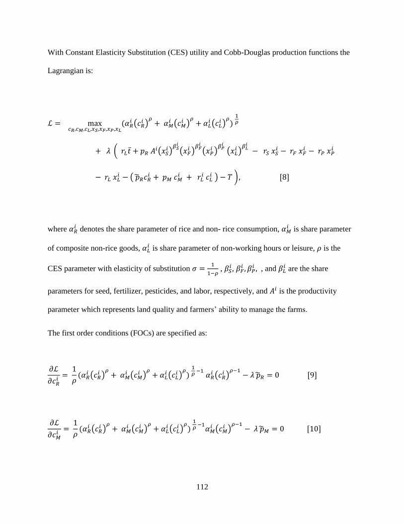
112
With Constant Elasticity Substitution (CES) utility and Cobb-Douglas production functions the
Lagrangian is:
ℒ = max𝑐𝑅,𝑐𝑀,𝑐𝐿,𝑥𝑆,𝑥𝐹,𝑥𝑃,𝑥𝐿
(𝛼𝑅𝑖 (𝑐𝑅
𝑖 )𝜌
+ 𝛼𝑀𝑖 (𝑐𝑀
𝑖 )𝜌
+ 𝛼𝐿𝑖 (𝑐𝐿
𝑖 )𝜌
) 1𝜌
+ 𝜆 ( 𝑟𝐿𝑡̅ + 𝑝𝑅 𝐴𝑖(𝑥𝑆𝑖 )
𝛽𝑆𝑖
(𝑥𝐹𝑖 )
𝛽𝐹𝑖
(𝑥𝑃𝑖 )
𝛽𝑃𝑖
(𝑥𝐿𝑖 )
𝛽𝐿𝑖
− 𝑟𝑆 𝑥𝑆𝑖 − 𝑟𝐹 𝑥𝐹
𝑖 − 𝑟𝑃 𝑥𝑃𝑖
− 𝑟𝐿 𝑥𝐿𝑖 − ( �̃�𝑅𝑐𝑅
𝑖 + 𝑝𝑀 𝑐𝑀𝑖 + 𝑟𝐿
𝑖 𝑐𝐿𝑖 ) − 𝑇 ), [8]
where 𝛼𝑅𝑖 denotes the share parameter of rice and non- rice consumption, 𝛼𝑀
𝑖 is share parameter
of composite non-rice goods, 𝛼𝐿𝑖 is share parameter of non-working hours or leisure, 𝜌 is the
CES parameter with elasticity of substitution 𝜎 =1
1−𝜌 , 𝛽𝑆
𝑖, 𝛽𝐹𝑖 , 𝛽𝑃
𝑖 , , and 𝛽𝐿𝑖 are the share
parameters for seed, fertilizer, pesticides, and labor, respectively, and 𝐴𝑖 is the productivity
parameter which represents land quality and farmers’ ability to manage the farms.
The first order conditions (FOCs) are specified as:
𝜕ℒ
𝜕𝑐𝑅𝑖
= 1
𝜌(𝛼𝑅
𝑖 (𝑐𝑅𝑖 )
𝜌+ 𝛼𝑀
𝑖 (𝑐𝑀𝑖 )
𝜌+ 𝛼𝐿
𝑖 (𝑐𝐿𝑖 )
𝜌)
1𝜌
−1 𝛼𝑅
𝑖 (𝑐𝑅𝑖 )
𝜌−1− 𝜆 �̃�𝑅 = 0 [9]
𝜕ℒ
𝜕𝑐𝑀𝑖
= 1
𝜌(𝛼𝑅
𝑖 (𝑐𝑅𝑖 )
𝜌+ 𝛼𝑀
𝑖 (𝑐𝑀𝑖 )
𝜌+ 𝛼𝐿
𝑖 (𝑐𝐿𝑖 )
𝜌)
1𝜌
−1𝛼𝑀
𝑖 (𝑐𝑀𝑖 )
𝜌−1− 𝜆 �̃�𝑀 = 0 [10]

113
𝜕ℒ
𝜕𝑐𝐿𝑖
= 1
𝜌(𝛼𝑅
𝑖 (𝑐𝑅𝑖 )
𝜌+ 𝛼𝑀
𝑖 (𝑐𝑀𝑖 )
𝜌+ 𝛼𝐿
𝑖 (𝑐𝐿𝑖 )
𝜌)
1𝜌
−1𝛼𝐿
𝑖 (𝑐𝐿𝑖 )
𝜌−1− 𝜆 𝑟𝐿 = 0 [11]
𝜕ℒ
𝜕𝑥𝑆𝑖
= 𝑝𝑅 𝛽𝑆𝑖𝐴(𝑥𝑆
𝑖 )𝛽𝑆
𝑖 −1(𝑥𝐹
𝑖 )𝛽𝐹
𝑖
(𝑥𝑃𝑖 )
𝛽𝑃𝑖
(𝑥𝐿𝑖 )
𝛽𝐿𝑖
− 𝑟𝑆 = 0 [12]
𝜕ℒ
𝜕𝑥𝐹𝑖
= 𝑝𝑅 𝛽𝐹𝑖 𝐴(𝑥𝑆
𝑖 )𝛽𝑆
𝑖
(𝑥𝐹𝑖 )
𝛽𝐹𝑖 −1
(𝑥𝑃𝑖 )
𝛽𝑃𝑖
(𝑥𝐿𝑖 )
𝛽𝐿𝑖
− 𝑟𝐹 = 0 [13]
𝜕ℒ
𝜕𝑥𝑃𝑖
= 𝑝𝑅 𝛽𝑃𝑖 𝐴(𝑥𝑆
𝑖 )𝛽𝑆
𝑖
(𝑥𝐹𝑖 )
𝛽𝐹𝑖
(𝑥𝑃𝑖 )
𝛽𝑃𝑖 −1
(𝑥𝐿𝑖 )
𝛽𝐿𝑖
– 𝑟𝑃 = 0 [14]
𝜕ℒ
𝜕𝑥𝐿𝑖
= 𝑝𝑅 𝛽𝐿𝑖 𝐴(𝑥𝑆
𝑖 )𝛽𝑆
𝑖
(𝑥𝐹𝑖 )
𝛽𝐹𝑖
(𝑥𝑃𝑖 )
𝛽𝑃𝑖
(𝑥𝐿𝑖 )
𝛽𝐿𝑖 −1
− 𝑟𝐿 = 0 [15]
𝜕ℒ
𝜕𝜆= 𝑟𝐿𝑡̅ + 𝑝𝑅 𝐴(𝑥𝑆
𝑖 )𝛽𝑆
𝑖
(𝑥𝐹𝑖 )
𝛽𝐹𝑖
(𝑥𝑃𝑖 )
𝛽𝑃𝑖
(𝑥𝐿𝑖 )
𝛽𝐿𝑖
− 𝑟𝑆 𝑥𝑆𝑖 − 𝑟𝐹 𝑥𝐹
𝑖 − 𝑟𝑃 𝑥𝑃𝑖 − 𝑟𝐿 𝑥𝐿
𝑖
− ( �̃�𝑅𝑐𝑅𝑖 + 𝑝𝑀 𝑐𝑀
𝑖 + 𝑟𝐿𝑖 𝑐𝐿
𝑖 ) − 𝑇 [16]

114
Eliminating 𝜆 by dividing 𝜕ℒ
𝜕𝑐𝑅𝑖 and
𝜕ℒ
𝜕𝑐𝑀𝑖 by
𝜕ℒ
𝜕𝑐𝐿𝑖 :
After eliminating 𝜆 (the FOCs of eliminating 𝜆 is provided in Appendix 4.2)
and simplification, the FOCs are as follows:
𝜕ℒ
𝜕𝑐𝑅𝑖
𝜕ℒ
𝜕𝑐𝐿𝑖
=
1𝜌 (𝛼𝑅
𝑖 (𝑐𝑅𝑖 )
𝜌+ 𝛼𝑀
𝑖 (𝑐𝑀𝑖 )
𝜌+ 𝛼𝐿
𝑖 (𝑐𝐿𝑖 )
𝜌)
1𝜌
−1 𝛼𝑅
𝑖 (𝑐𝑅𝑖 )
𝜌−1
1𝜌 (𝛼𝑅
𝑖 (𝑐𝑅𝑖 )
𝜌+ 𝛼𝑀
𝑖 (𝑐𝑀𝑖 )
𝜌+ 𝛼𝐿
𝑖 (𝑐𝐿𝑖 )
𝜌)
1𝜌
−1𝛼𝐿
𝑖 (𝑐𝐿𝑖 )
𝜌−1−
𝜆 �̃�𝑅
𝜆 𝑟𝐿= 0 [17]
𝜕ℒ
𝜕𝑐𝑀𝑖
𝜕ℒ
𝜕𝑐𝐿𝑖
=
1𝜌 (𝛼𝑅
𝑖 (𝑐𝑅𝑖 )
𝜌+ 𝛼𝑀
𝑖 (𝑐𝑀𝑖 )
𝜌+ 𝛼𝐿
𝑖 (𝑐𝐿𝑖 )
𝜌)
1𝜌
−1𝛼𝑀
𝑖 (𝑐𝑀𝑖 )
𝜌−1
1𝜌
(𝛼𝑅𝑖 (𝑐𝑅
𝑖 )𝜌
+ 𝛼𝑀𝑖 (𝑐𝑀
𝑖 )𝜌
+ 𝛼𝐿𝑖 (𝑐𝐿
𝑖 )𝜌
) 1𝜌
−1𝛼𝐿
𝑖 (𝑐𝐿𝑖 )
𝜌−1−
𝜆 �̃�𝑀
𝜆 𝑟𝐿= 0 [18]
𝜕ℒ
𝜕𝑥𝑆𝑖
= 𝑝𝑅 𝛽𝑆𝑖𝐴(𝑥𝑆
𝑖 )𝛽𝑆
𝑖 −1(𝑥𝐹
𝑖 )𝛽𝐹
𝑖
(𝑥𝑃𝑖 )
𝛽𝑃𝑖
(𝑥𝐿𝑖 )
𝛽𝐿𝑖
− 𝑟𝑆 = 0 [19]
𝜕ℒ
𝜕𝑥𝐹𝑖
= 𝑝𝑅 𝛽𝐹𝑖 𝐴(𝑥𝑆
𝑖 )𝛽𝑆
𝑖
(𝑥𝐹𝑖 )
𝛽𝐹𝑖 −1
(𝑥𝑃𝑖 )
𝛽𝑃𝑖
(𝑥𝐿𝑖 )
𝛽𝐿𝑖
− 𝑟𝐹 = 0 [20]
𝜕ℒ
𝜕𝑥𝑃𝑖
= 𝑝𝑅 𝛽𝑃𝑖 𝐴(𝑥𝑆
𝑖 )𝛽𝑆
𝑖
(𝑥𝐹𝑖 )
𝛽𝐹𝑖
(𝑥𝑃𝑖 )
𝛽𝑃𝑖 −1
(𝑥𝐿𝑖 )
𝛽𝐿𝑖
− 𝑟𝑃 = 0 [21]

115
𝜕ℒ
𝜕𝑥𝐿𝑖
= 𝑝𝑅 𝛽𝐿𝑖 𝐴(𝑥𝑆
𝑖 )𝛽𝑆
𝑖
(𝑥𝐹𝑖 )
𝛽𝐹𝑖
(𝑥𝑃𝑖 )
𝛽𝑃𝑖
(𝑥𝐿𝑖 )
𝛽𝐿𝑖 −1
− 𝑟𝐿 = 0 [22]
𝜕ℒ
𝜕𝜆= 𝑟𝐿𝑡̅ + 𝑝𝑅 𝐴(𝑥𝑆
𝑖 )𝛽𝑆
𝑖
(𝑥𝐹𝑖 )
𝛽𝐹𝑖
(𝑥𝑃𝑖 )
𝛽𝑃𝑖
(𝑥𝐿𝑖 )
𝛽𝐿𝑖
− 𝑟𝑆 𝑥𝑆𝑖 − 𝑟𝐹 𝑥𝐹
𝑖 − 𝑟𝑃 𝑥𝑃𝑖 − 𝑟𝐿 𝑥𝐿
𝑖
− ( �̃�𝑅𝑐𝑅𝑖 + 𝑝𝑀 𝑐𝑀
𝑖 + 𝑟𝐿 𝑐𝐿𝑖 ) − 𝑇 = 0 [23]
Further simplification of FOCs yields:
𝛼𝑅
𝑖
𝛼𝐿𝑖
(𝑐𝑅
𝑖
𝑐𝐿𝑖)
𝜌−1
= �̃�𝑅
𝑟𝐿 [24]
𝛼𝑀
𝑖
𝛼𝐿𝑖
(𝑐𝑀
𝑖
𝑐𝐿𝑖
)
𝜌−1
= �̃�𝑀
𝑟𝐿 [25]
𝑝𝑅 𝛽𝑆𝑖𝐴(𝑥𝑆
𝑖 )𝛽𝑆
𝑖 −1(𝑥𝐹
𝑖 )𝛽𝐹
𝑖
(𝑥𝑃𝑖 )
𝛽𝑃𝑖
(𝑥𝐿𝑖 )
𝛽𝐿𝑖
= 𝑟𝑆 [26]
𝑝𝑅 𝛽𝐹𝑖 𝐴(𝑥𝑆
𝑖 )𝛽𝑆
𝑖
(𝑥𝐹𝑖 )
𝛽𝐹𝑖 −1
(𝑥𝑃𝑖 )
𝛽𝑃𝑖
(𝑥𝐿𝑖 )
𝛽𝐿𝑖
= 𝑟𝐹 [27]
𝑝𝑅 𝛽𝑃𝑖 𝐴(𝑥𝑆
𝑖 )𝛽𝑆
𝑖
(𝑥𝐹𝑖 )
𝛽𝐹𝑖
(𝑥𝑃𝑖 )
𝛽𝑃𝑖 −1
(𝑥𝐿𝑖 )
𝛽𝐿𝑖
= 𝑟𝑃 [28]

116
𝑝𝑅 𝛽𝐿𝑖 𝐴(𝑥𝑆
𝑖 )𝛽𝑆
𝑖
(𝑥𝐹𝑖 )
𝛽𝐹𝑖
(𝑥𝑃𝑖 )
𝛽𝑃𝑖
(𝑥𝐿𝑖 )
𝛽𝐿𝑖 −1
= 𝑟𝐿 [29]
𝑟𝐿𝑡̅ + 𝑝𝑅 𝐴(𝑥𝑆𝑖 )
𝛽𝑆 𝑖
(𝑥𝐹𝑖 )
𝛽𝐹𝑖
(𝑥𝑃𝑖 )
𝛽𝑃𝑖
(𝑥𝐿𝑖 )
𝛽𝐿𝑖
− 𝑟𝑆 𝑥𝑆𝑖 − 𝑟𝐹 𝑥𝐹
𝑖 − 𝑟𝑃 𝑥𝑃𝑖 − 𝑟𝐿 𝑥𝐿
𝑖
= ( �̃�𝑅𝑐𝑅𝑖 + 𝑝𝑀 𝑐𝑀
𝑖 + 𝑟𝐿 𝑐𝐿𝑖 ) − 𝑇. [30]
Equations [24] – [30] represent a system of seven equations in seven endogenous variables
𝑐𝑅 , 𝑐𝑀, 𝑐𝐿 , 𝑥𝑆, 𝑥𝐹 , 𝑥𝑃, 𝑥𝐿. To simplify the empirical analysis, analytical solution for the input
demand function, income, and consumer demand functions are solved for using this system of
seven equations. Solving equations [26] – [29] simultaneously yields input demand functions:
𝑥𝑆𝑖 (𝑝𝑅, 𝑟𝑆, 𝑟𝐹 , 𝑟𝑃, 𝑟𝐿) = (𝑝𝑅𝐴)
1
1−𝛽𝑆𝑖 −𝛽𝐹
𝑖 −𝛽𝑃𝑖 −𝛽𝐿
𝑖(
𝛽𝑆𝑖
𝑟𝑆)
1−𝛽𝐹𝑖 −𝛽𝑃
𝑖 −𝛽𝐿𝑖
1−𝛽𝑆𝑖 −𝛽𝐹
𝑖 −𝛽𝑃𝑖 −𝛽𝐿
𝑖
(𝛽𝐹
𝑖
𝑟𝐹)
𝛽𝐹𝑖
1−𝛽𝑆𝑖 −𝛽𝐹
𝑖 −𝛽𝑃𝑖 −𝛽𝐿
𝑖
(𝛽𝑃
𝑖
𝑟𝑃)
𝛽𝑃𝑖
1−𝛽𝑆𝑖 −𝛽𝐹
𝑖 −𝛽𝑃𝑖 −𝛽𝐿
𝑖
(𝛽𝐿
𝑖
𝑟𝐿)
𝛽𝐿𝑖
1−𝛽𝑆𝑖 −𝛽𝐹
𝑖 −𝛽𝑃𝑖 −𝛽𝐿
𝑖
[31]
𝑥𝐹𝑖 (𝑝𝑅 , 𝑟𝑆, 𝑟𝐹, 𝑟𝑃, 𝑟𝐿) = (𝑝𝑅𝐴)
1
1−𝛽𝑆𝑖 −𝛽𝐹
𝑖 −𝛽𝑃𝑖 −𝛽𝐿
𝑖(
𝛽𝐹𝑖
𝑟𝐹)
1−𝛽𝑆𝑖 −𝛽𝑃
𝑖 −𝛽𝐿𝑖
1−𝛽𝑆𝑖 −𝛽𝐹
𝑖 −𝛽𝑃𝑖 −𝛽𝐿
𝑖
(𝛽𝑆
𝑖
𝑟𝑆)
𝛽𝑆𝑖
1−𝛽𝑆𝑖 −𝛽𝐹
𝑖 −𝛽𝑃𝑖 −𝛽𝐿
𝑖
(𝛽𝑃
𝑖
𝑟𝑃)
𝛽𝑃𝑖
1−𝛽𝑆𝑖 −𝛽𝐹
𝑖 −𝛽𝑃𝑖 −𝛽𝐿
𝑖
(𝛽𝐿
𝑖
𝑟𝐿)
𝛽𝐿𝑖
1−𝛽𝑆𝑖 −𝛽𝐹
𝑖 −𝛽𝑃𝑖 −𝛽𝐿
𝑖
[32]

117
𝑥𝑃𝑖 (𝑝𝑅, 𝑟𝑆, 𝑟𝐹 , 𝑟𝑃, 𝑟𝐿) = (𝑝𝑅𝐴)
1
1−𝛽𝑆𝑖 −𝛽𝐹
𝑖 −𝛽𝑃𝑖 −𝛽𝐿
𝑖(
𝛽𝑃𝑖
𝑟𝑃)
1−𝛽𝑆𝑖 −𝛽𝐹
𝑖 −𝛽𝐿𝑖
1−𝛽𝑆𝑖 −𝛽𝐹
𝑖 −𝛽𝑃𝑖 −𝛽𝐿
𝑖
(𝛽𝐹
𝑖
𝑟𝐹)
𝛽𝐹𝑖
1−𝛽𝑆𝑖 −𝛽𝐹
𝑖 −𝛽𝑃𝑖 −𝛽𝐿
𝑖
(𝛽𝑆
𝑖
𝑟𝑆)
𝛽𝑆𝑖
1−𝛽𝑆𝑖 −𝛽𝐹
𝑖 −𝛽𝑃𝑖 −𝛽𝐿
𝑖
(𝛽𝐿
𝑖
𝑟𝐿)
𝛽𝐿𝑖
1−𝛽𝑆𝑖 −𝛽𝐹
𝑖 −𝛽𝑃𝑖 −𝛽𝐿
𝑖
[33]
𝑥𝐿𝑖 (𝑝𝑅, 𝑟𝑆, 𝑟𝐹 , 𝑟𝑃, 𝑟𝐿) = (𝑝𝑅𝐴)
1
1−𝛽𝑆𝑖 −𝛽𝐹
𝑖 −𝛽𝑃𝑖 −𝛽𝐿
𝑖(
𝛽𝐿𝑖
𝑟𝐿)
1−𝛽𝑆𝑖 −𝛽𝐹
𝑖 −𝛽𝑃𝑖
1−𝛽𝑆𝑖 −𝛽𝐹
𝑖 −𝛽𝑃𝑖 −𝛽𝐿
𝑖
(𝛽𝐹
𝑖
𝑟𝐹)
𝛽𝐹𝑖
1−𝛽𝑆𝑖 −𝛽𝐹
𝑖 −𝛽𝑃𝑖 −𝛽𝐿
𝑖
(𝛽𝑃
𝑖
𝑟𝑃)
𝛽𝑃𝑖
1−𝛽𝑆𝑖 −𝛽𝐹
𝑖 −𝛽𝑃𝑖 −𝛽𝐿
𝑖
(𝛽𝐿
𝑖
𝑟𝐿)
𝛽𝑆𝑖
1−𝛽𝑆𝑖 −𝛽𝐹
𝑖 −𝛽𝑃𝑖 −𝛽𝐿
𝑖
[34]
With analytical solutions for the input demand functions, income 𝑌 is fully defined by left-hand
side of equation [30] for given output and input prices:
𝑌(𝑝𝑅, 𝑟𝑆, 𝑟𝐹, 𝑟𝑃, 𝑟𝐿) = 𝑟𝐿𝑡̅ + 𝑝𝑅 𝐴 (𝑥𝑆𝑖 (∙))
𝛽𝑆 𝑖
(𝑥𝐹𝑖 (∙))
𝛽𝐹𝑖
(𝑥𝑃𝑖 (∙))
𝛽𝑃𝑖
(𝑥𝐿𝑖 (∙))
𝛽𝐿𝑖
− 𝑟𝑆 𝑥𝑆𝑖 (∙) − 𝑟𝐹 𝑥𝐹
𝑖 (∙) − 𝑟𝑃 𝑥𝑃𝑖 (∙) − 𝑟𝐿 𝑥𝐿
𝑖 (∙). [35]
Then given income, solving equations [24], [25], and [30] simultaneously yields consumer
demand functions:
𝑐𝑅𝑖 ( �̃�𝑅, 𝑝𝑀, 𝑟𝐿 , 𝑌) = (
𝛼𝑅𝑖
�̃�𝑅)
𝜌𝑌(𝑝𝑅 , 𝑟𝑆, 𝑟𝐹, 𝑟𝑃, 𝑟𝐿)
(𝛼𝑅𝑖 )
𝜌( �̃�𝑅)1−𝜌
+

118
(𝛼𝑀𝑖 )
𝜌(𝑝𝑀)(1−𝜌) + (𝛼𝐿
𝑖 )𝜌
( 𝑟𝐿)(1−𝜌) [36]
𝑐𝑀𝑖 ( �̃�𝑅, 𝑝𝑀, 𝑟𝐿 , 𝑌) = (
𝛼𝑀𝑖
𝑝𝑀)
𝜌𝑌(𝑝𝑅 , 𝑟𝑆, 𝑟𝐹, 𝑟𝑃, 𝑟𝐿)
(𝛼𝑅𝑖 )
𝜌( �̃�𝑅)1−𝜌
+
(𝛼𝑀𝑖 )
𝜌(𝑝𝑀)(1−𝜌) + (𝛼𝐿
𝑖 )𝜌
( 𝑟𝐿)(1−𝜌) [37]
𝑐𝐿𝑖 ( �̃�𝑅 , 𝑝𝑀, 𝑟𝐿 , 𝑌) = (
𝛼𝐿𝑖
𝑟𝐿)
𝜌𝑌(𝑝𝑅 , 𝑟𝑆, 𝑟𝐹 , 𝑟𝑃, 𝑟𝐿)
(𝛼𝑅𝑖 )
𝜌( �̃�𝑅)1−𝜌
+
(𝛼𝑀𝑖 )
𝜌(𝑝𝑀)(1−𝜌) + (𝛼𝐿
𝑖 )𝜌
( 𝑟𝐿)(1−𝜌) [38]
The above model defines a system of 8 equations (equations [31] – [38]) in 8 endogenous
variables ( 𝑥𝑆𝑖 (∙), 𝑥𝐹
𝑖 (∙), 𝑥𝑃𝑖 (∙), 𝑥𝐿
𝑖 (∙), 𝑌(∙), 𝑐𝑅𝑖 (∙), 𝑐𝑀
𝑖 (∙), 𝑐𝐿𝑖 (∙)) that are implemented to quantify
the effect of free trade policy—through changes in the producer price of paddy rice (𝑝𝑅) and
consumer price of milled rice ( �̃�𝑅)—on individual rice farmers’ production and consumption.
With production and consumption impacts quantified, we can analyze how free trade affects the
poverty and welfare of farmers, which are defined next.
Poverty is defined using both monetary and non-monetary measures through examining
household incomes and rice consumption. Individual household income levels are compared to
Malaysia’s current national Poverty Line Income (PLI) which is specified, for a household of six,
as a total annual income of RM 9,600 (US$ 2,238) for poor and RM 5,520 (US$ 1,287) for
extreme poor. However, a sole income indicator will not capture the household’s standard of

119
living when the price of rice falls under free trade; these drawbacks indicate that consumption is
a better predictor of derivation than income (Meyer and Sullivan 2003, 2011). Thus, as a
compliment to the income-based poverty measure, a consumption-based measure is defined as
the quantity of rice consumed per person that is below the per capita consumption average of
88.9 kg. We quantify the percentage of households with: a) earnings below the two income
levels and b) per person rice consumption below the per capita average before and after free
trade. The poverty measurements among rice farm households help Malaysia, as a developing
country, to gauge farm program effectiveness and guide policy development strategy. Since
neither of the individual poverty measures fully represent a household’s welfare, a complete
welfare measurement is considered next.
With the CES utility function defined in equation [8] being homogeneous of degree
one,30 it gives the real income index of rice farmer household 𝑖. Calculating the percentage
change in real income before and after the free trade policy provides the equivalent variation
30 The utility function is homogeneous of degree one if it satisfies the
condition: 𝑈 (𝑆𝑐𝑅𝑖 , 𝑆𝑐𝑀
𝑖 , 𝑆𝑐𝐿𝑖 ) = 𝑆1𝑈 (𝑐𝑅
𝑖 , 𝑐𝑀𝑖 , 𝑐𝐿
𝑖 ), where 𝑆 is a constant. Thus, scaling utility in
equation [8] by 𝑆 gives:
𝑈 (𝑆𝑐𝑅𝑖 , 𝑆𝑐𝑀
𝑖 , 𝑆𝑐𝐿𝑖 ) = (𝛼𝑅
𝑖 (𝑆𝑐𝑅𝑖 )
𝜌+ 𝛼𝑀
𝑖 (𝑆𝑐𝑀𝑖 )
𝜌+ 𝛼𝐿
𝑖 (𝑆𝑐𝐿𝑖 )
𝜌)
1𝜌
= (𝑆𝜌𝛼𝑅𝑖 (𝑐𝑅
𝑖 )𝜌
+ 𝑆𝜌𝛼𝑀𝑖 (𝑐𝑀
𝑖 )𝜌
+ 𝑆𝜌𝛼𝐿𝑖 (𝑐𝐿
𝑖 )𝜌
) 1𝜌
= 𝑆𝜌
1𝜌(𝛼𝑅
𝑖 (𝑐𝑅𝑖 )
𝜌+ 𝛼𝑀
𝑖 (𝑐𝑀𝑖 )
𝜌+ 𝛼𝐿
𝑖 (𝑐𝐿𝑖 )
𝜌)
1𝜌
= 𝑆1(𝛼𝑅𝑖 (𝑐𝑅
𝑖 )𝜌
+ 𝛼𝑀𝑖 (𝑐𝑀
𝑖 )𝜌
+ 𝛼𝐿𝑖 (𝑐𝐿
𝑖 )𝜌
) 1𝜌.
Thus, the utility function is homogeneous of degree one.

120
welfare measure for each household. Equivalent variation measures the change in wealth under
baseline prices that would have the same consumer welfare effect with free trade prices holding
income constant at the baseline level.
3. Data and Model Calibration
This section discusses data and sources, estimation of probability density functions,
sampling technique for utility and production share parameters, and calibration method for the
remaining parameters.
3.1 Data Integration
To parameterize and calibrate the model, this study integrates and utilizes three different
farm household surveys on rice farming and production in Malaysia that were conducted by the
Malaysian Agricultural Research and Development Institute (MARDI). These surveys were
designed with different research objectives and in different production periods to help
researchers analyze the rice policy issues of self-sufficiency and food security. In doing so, the
studies provide key information on the heterogeneity among rice farmers. Since one of goals of
this study is to analyze farm incomes and expenditure, these surveys are useful to calibrate the
individual-specific parameters in the model. Focusing on major rice production areas, each
survey details different aspects of rice farmers’ finances: farm household income and
expenditures and farm household production expenditures.
3.1.1 Farm Household Expenditure and Income Survey
The Farm Household Expenditure and Income Survey (HIES) was conducted by research
associates from MARDI and trained enumerators from Muda Agriculture Development
Authority (MADA) and Kemubu Agriculture Development Authority (KADA) in 2012/2013

121
production years (Rabu and Mohd Shah, 2013). This survey covered 123 rice farmers
represented as the head of the household in three (IADA Barat Laut Selangor, MADA, and
KADA) out of eight major areas of rice production in Malaysia. Summary statistics from this
survey are reported in Table 4.18. From this survey, the number of household members,
household incomes, and household expenditure are important variables used in the model
calibration discussed in detail below.
Table 4.18: Selected variables on farm household expenditure and income survey.
Regions Mean Min. Max. Std. Dev.
Household Size
PBLS
MADA
KADA
Average
6
5
5
5
1
1
1
1
9
5
9
8
2
1
1
2
Household Gross Income from Rice Activities (RM/Month)
PBLS
MADA
KADA
Average
1,401
1,267
1,358
1,342
500
250
350
367
7,000
7,000
3,000
5,667
1,110.2
1,214.3
723.6
1,016.0
Household Income from Other Sources (RM/Month)
PBLS
MADA
KADA
Average
600
300
350
417
260
180
170
203
764
539
450
584
160.3
130.7
140.6
143.9
Household Expenditure for Food (RM/Month)
PBLS
MADA
KADA
Average
625.5
590.4
578.7
598.2
120
250
100
157
2,000
1,500
1,200
1,567
317.2
277.2
286.8
293.7
Source: Malaysian Agricultural Research and Development Institute.

122
3.1.2 Farm Production Expenditure Survey
The Farm Production Expenditure Survey was conducted in the 2016 production year and
focused on major production areas including MADA and the Integrated Agriculture
Development Area (IADA) Penang. A total of 120 rice farmers from these regions were
randomly selected. The main objective of the survey was to obtain the production costs and
expenditures from the sampled rice farms (Table 4.19). From this survey, acreage, yield,
production input costs for seed, fertilizer, pesticide, herbicide, labor, and land were used in the
model calibration.
Table 4.19: Selected variables on farm production expenditure survey.
Regions Mean Min. Max. Std. Dev.
Acreage (Ha)
MADA 2.09 0.29 17.40 2.46
IADA Penang 3.47 0.20 21.40 4.50
Average 2.78 0.25 19.40 3.48 Yield (MT/Ha)
MADA 6.36 2.96 8.68 1.37
IADA Penang 6.57 2.25 11.22 2.02
Average 6.47 2.61 9.95 1.70 Seed Cost (RM/Ha) *
MADA 282.48 122.50 347.22 29.90
IADA Penang 629.20 223.20 1,125.00 233.92
Average 455.84 172.85 736.11 131.91 Fertilizer Cost (RM/Ha) *
MADA 85.50 30.00 156.39 35.66
IADA Penang 87.50 38.00 156.00 49.43
Average 86.50 34.00 156.20 42.54 Pesticide Cost (RM/Ha) *
MADA 298.49 207.00 478.01 95.96
IADA Penang 447.99 200.00 953.00 237.08
Average 373.24 203.50 715.50 166.52

123
Table 4.19 (Cont.)
Regions Mean Min. Max. Std. Dev.
Herbicide Cost (RM/Ha)
MADA 256.47 0.00 555.00 137.30
IADA Penang 142.65 48.00 480.00 109.22
Average 199.56 24.00 517.50 123.26 Labor Cost (RM/Ha)
MADA 566.20 250.00 1,014.50 239.20
IADA Penang 722.56 250.00 2,030.00 448.40
Average 644.38 250.00 1,522.25 343.80 Land Rental Cost (RM/Ha)
MADA 1,733.78 1042.50 2,780.00 372.75
IADA Penang 883.00 159.00 1,574.00 305.67
Average 1,308.39 600.75 2,177.00 339.21
* Costs are excluded subsidies.
Source: Malaysian Agricultural Research and Development Institute.
3.1.3 Farm Household Income Survey
The Farm Household Income Survey (HIS) sampled 250 rice farmers from MADA,
Integrated Agriculture Development Area (IADA) Penang, IADA Kemasin, IADA KETARA,
and KADA and was conducted in 2015/16 production years. Key variables collected include the
main sources of farm household income and working hours on rice farm activities, which are
also the essential variables for model calibration (Table 4.20).
Table 4.20: Selected variables of farm household income survey.
Regions Mean Min. Max. Std. Dev.
Main Source of Income*
MADA
IADA Penang
IADA Kemasin
IADA KETARA
KADA
Average
1
2
1
1
1
1
1
1
1
1
1
1
6
6
4
4
5
5
1.218
1.612
0.761
0.636
1.039
1.053

124
Table 4.20 (Cont.)
Regions Mean Min. Max. Std. Dev.
Working Hours of Rice Activities (Hrs.)
MADA
IADA Penang
IADA Kemasin
IADA KETARA
KADA
Average
5.1
5.5
5.6
6.2
6.4
5.7
1.0
0.0
2.0
2.0
2.0
1.4
10.0
9.0
8.0
11.0
11.0
9.8
1.635
2.351
1.752
1.861
2.164
1.953 *1=Rice farms, 2=Non-rice farms, 3=Own business, 4=Public service, 5=Private Service.
Source: Malaysian Agricultural Research and Development Institute (2015/16).
3.2 Distribution Estimations of Share Parameters
For individual farmers, the data from the three surveys are used to calibrate the share
parameters in the utility function (𝛼𝑅𝑖 and 𝛼𝑀
𝑖 ) and production function (𝛽𝑆𝑖, 𝛽𝐹
𝑖 , 𝛽𝑃𝑖 , and 𝛽𝐿
𝑖 ).
Share parameters in the utility function are household expenditures on consumption goods (rice
or non-rice) divided by total consumption expenditure. Share parameters in the production
function are farm expenditures on individual input (seed, fertilizer, pesticide, and labor) divided
by total farm expenditures. Since observations across surveys do not track the same rice farmer
(i.e. households) with different sample sizes, the data cannot be used directly from the surveys to
calibrate these share parameters for each individual farmer. Therefore, the survey data is used to
estimate the distributions for each share parameter using maximum likelihood estimation (MLE).
MLE, which finds the parameter values that maximize the likelihood of given the observed
sample, is applied to estimate the parameters for a univariate probability density function (PDF)
of each of the utility and production share parameters. Then, utilizing correlation matrices, the
multivariate simulation approach developed by Phoon et al. (2004) is applied to randomly draw
correlated share parameters from the univariate distribution to accurately reflect the survey data.

125
3.2.1 Probability Density Function and Maximum Likelihood Estimation
For both utility and production share parameters, distributions are estimated using log-
likelihood functions and the MLE procedure. The log-likelihood functions are derived for the
Normal, Log-normal, Beta, Gamma, truncated, and mixture distributions. Then, AIC and BIC
statistics and graphical analysis, are employed to determine the distribution that best fits the data.
The PDF used to estimate share parameters are as follow:
(i) Normal Density Function:
For the random variable 𝑥 ∈ [−∞, ∞], the equation for the normal distribution is:
𝑓(𝑥) = 1
√2𝜋2 𝑒
−(𝑥−𝜇)2
2𝜎2 ,
where 𝜇 ∈ [−∞, ∞] is the mean and 𝜎2 > 0 is the variance.
(ii) Log-normal Density Function:
For the random variable 𝑥 ∈ [0, ∞], the equation for the log-normal distribution is:
𝑓(𝑥) = 1
𝑥𝜎√2𝜋 𝑒
−(𝑙𝑛𝑥−𝜇)2
2𝜎2 ,
where 𝜇 ∈ [−∞, ∞] is the mean and 𝜎 > 0 is the variance.
(iii) Beta Density Function:
For the random variable 𝑥 ∈ [0,1], the equation for the Beta distribution is:

126
𝑓(𝑥) = (𝑥)𝛼−1 (1 − 𝑥)𝛽−1
𝐵(𝛼, 𝛽) ,
where 𝛼 > 0 and 𝛽 > 0 are both shape parameters.
(iv) Gamma Density Function:
For the random variable 𝑥 ∈ [0, ∞], the equation for the Gamma distribution is:
𝑓(𝑥) =1
Γ(𝑘)𝜃𝑘 𝑥𝑘−1𝑒−
𝑥𝜃,
where 𝑘 > 0 is shape and 𝜃 > 0 is scale.
(v) Truncated Density Function:
A truncated distribution results from a restriction on the support of a probability density
function. Since share parameters are restricted to values between zero and one (i.e., 0 < x < 1),
truncated distributions are used to limit support of the densities with supports outside this range.
Truncated distributions are also a mathematically defensible way to preserve the main features of
distribution while avoiding extreme values for random samples where the support is infinite at
one or both ends (Burkardt, 2014). All PDFs can be truncated between a and b using the
following formula:
𝑇𝑟(𝑥) = {
𝑓(𝑥)
𝐹(𝑏) − 𝐹(𝑎) for 𝑎 < 𝑥 ≤ 𝑏
0 otherwise,
where 𝑓(𝑥) is the PDF and 𝐹 (∙) is the corresponding cumulative distribution function.

127
(vi) Mixture Density Function:
A mixture distribution refers to a probability distribution of random variables that is
derived from a mixture of two or more PDFs. Since some share parameters are bimodal (see
histograms presented below), mixture density in the PDF is used. For PDFs 𝑓1(𝑥), … , 𝑓𝑛(𝑥) and
weighting parameters 𝑤1, … , 𝑤𝑛 where 𝑤𝑖 > 0 for all i and ∑ 𝑤𝑛𝑖=1 𝑖
= 1, the mixture distribution
is defined as:
𝑓𝑚(𝑥) = ∑ 𝑤𝑖 𝑓𝑖(𝑥).
𝑛
𝑖=1
Next, the MLE procedure is discussed. After the likelihood function is defined based on
joint density functions, Newton’s method is applied to find the parameter values that maximize
the likelihood function given the data. The joint density function for an independent and
identically distributed sample is:
𝑓(𝑥1, 𝑥2, … . . , 𝑥𝑛 | 𝜃) = 𝑓(𝑥1| 𝜃 ) × 𝑓(𝑥2| 𝜃) × … .. × 𝑓(𝑥𝑛| 𝜃),
where 𝑥1, 𝑥2, … . . , 𝑥𝑛 are observed values and 𝜃 is a parameter vector. The likelihood
function is defined by considering the values 𝑥1, 𝑥2, … . . , 𝑥𝑛 to be fixed observations and
allowing 𝜃 to change freely. The likelihood function is:
ℒ (𝜃; 𝑥1, 𝑥2, … . . , 𝑥𝑛 ) = ∏ 𝑓(𝑥𝑖| 𝜃)
𝑛
𝑖=1
.
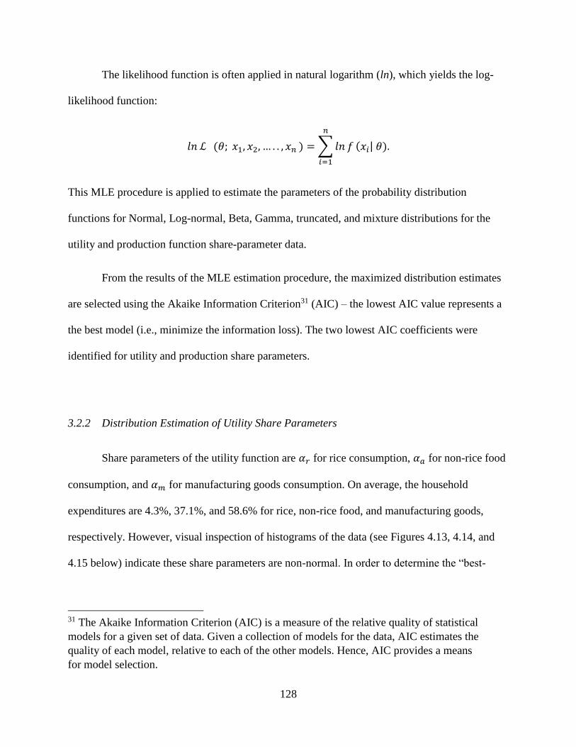
128
The likelihood function is often applied in natural logarithm (ln), which yields the log-
likelihood function:
𝑙𝑛 ℒ (𝜃; 𝑥1, 𝑥2, … . . , 𝑥𝑛 ) = ∑ 𝑙𝑛 𝑓 (𝑥𝑖| 𝜃).
𝑛
𝑖=1
This MLE procedure is applied to estimate the parameters of the probability distribution
functions for Normal, Log-normal, Beta, Gamma, truncated, and mixture distributions for the
utility and production function share-parameter data.
From the results of the MLE estimation procedure, the maximized distribution estimates
are selected using the Akaike Information Criterion31 (AIC) – the lowest AIC value represents a
the best model (i.e., minimize the information loss). The two lowest AIC coefficients were
identified for utility and production share parameters.
3.2.2 Distribution Estimation of Utility Share Parameters
Share parameters of the utility function are 𝛼𝑟 for rice consumption, 𝛼𝑎 for non-rice food
consumption, and 𝛼𝑚 for manufacturing goods consumption. On average, the household
expenditures are 4.3%, 37.1%, and 58.6% for rice, non-rice food, and manufacturing goods,
respectively. However, visual inspection of histograms of the data (see Figures 4.13, 4.14, and
4.15 below) indicate these share parameters are non-normal. In order to determine the “best-
31 The Akaike Information Criterion (AIC) is a measure of the relative quality of statistical
models for a given set of data. Given a collection of models for the data, AIC estimates the
quality of each model, relative to each of the other models. Hence, AIC provides a means
for model selection.
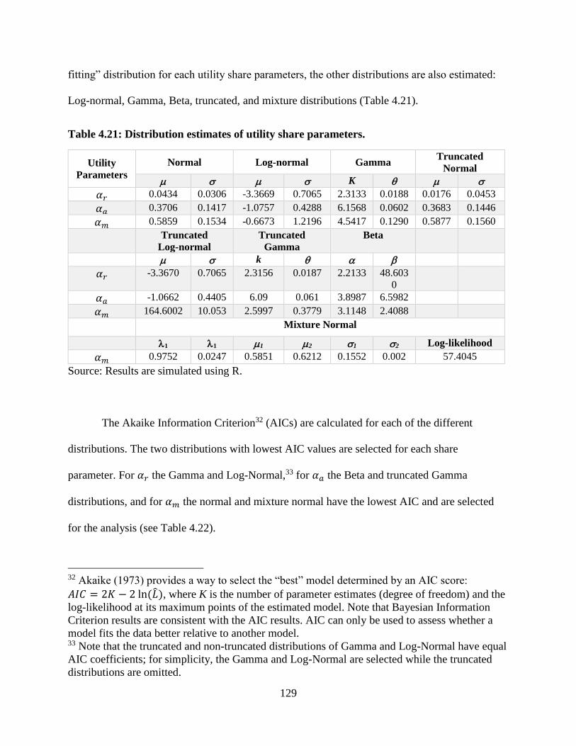
129
fitting” distribution for each utility share parameters, the other distributions are also estimated:
Log-normal, Gamma, Beta, truncated, and mixture distributions (Table 4.21).
Table 4.21: Distribution estimates of utility share parameters.
Utility
Parameters
Normal Log-normal Gamma Truncated
Normal
K
𝛼𝑟 0.0434 0.0306 -3.3669 0.7065 2.3133 0.0188 0.0176 0.0453
𝛼𝑎 0.3706 0.1417 -1.0757 0.4288 6.1568 0.0602 0.3683 0.1446
𝛼𝑚 0.5859 0.1534 -0.6673 1.2196 4.5417 0.1290 0.5877 0.1560
Truncated
Log-normal
Truncated
Gamma
Beta
k
𝛼𝑟 -3.3670 0.7065 2.3156 0.0187 2.2133 48.603
0
𝛼𝑎 -1.0662 0.4405 6.09 0.061 3.8987 6.5982
𝛼𝑚 164.6002 10.053 2.5997 0.3779 3.1148 2.4088
Mixture Normal
1 1 1 2 1 2 Log-likelihood
𝛼𝑚 0.9752 0.0247 0.5851 0.6212 0.1552 0.002 57.4045
Source: Results are simulated using R.
The Akaike Information Criterion32 (AICs) are calculated for each of the different
distributions. The two distributions with lowest AIC values are selected for each share
parameter. For 𝛼𝑟 the Gamma and Log-Normal,33 for 𝛼𝑎 the Beta and truncated Gamma
distributions, and for 𝛼𝑚 the normal and mixture normal have the lowest AIC and are selected
for the analysis (see Table 4.22).
32 Akaike (1973) provides a way to select the “best” model determined by an AIC score: 𝐴𝐼𝐶 = 2𝐾 − 2 ln (�̂�), where K is the number of parameter estimates (degree of freedom) and the
log-likelihood at its maximum points of the estimated model. Note that Bayesian Information
Criterion results are consistent with the AIC results. AIC can only be used to assess whether a
model fits the data better relative to another model. 33 Note that the truncated and non-truncated distributions of Gamma and Log-Normal have equal
AIC coefficients; for simplicity, the Gamma and Log-Normal are selected while the truncated
distributions are omitted.

130
Table 4.22: Results of AIC coefficients for utility share parameters.
Share
Parameters AIC and Distribution Estimations
𝛼𝑟 Truncated
Gamma
Gamma Truncated
Log-
normal
Log-
normal
Beta Truncated
Normal
Normal
-561.27 -561.27 -560.65 -560.65 -560.29 -540.28
-504.12
𝛼𝑎 Beta Truncated
Gamma
Truncated
Normal
Gamma Normal Truncated
Log-
normal
Log-
Normal
-130.47 -128.99 -128.85 -128.72 -127.64 -121.52 -119.84
𝛼𝑚 Truncated
Normal
Normal Mixture
Normal
Beta Truncated
Log-
normal
Gamma Truncated
Gamma
-109.01 -108.06 -102.80 -57.42 -15.16 16.30
16.30
Source: Results are simulated using R.
Finally, to assure the most precise distribution estimation for each share parameter,
graphical analysis is employed. Using the estimated parameters, the two probability density
functions (PDFs) with the lowest AICs are superimposed onto the histogram of the data. The
distribution that visually fits the data most accurately is used for the simulation analysis. Figure
4.13 provides the graphical analysis for 𝛼𝑟. Based on this figure, the Gamma distribution (blue
curve) most accurately fits the histogram, which is consistent with the AIC analysis. Therefore,
the Gamma is selected over the Log-normal (red curve) for the rice consumption share
parameter.

131
Source: Results are simulated using R.
Figure 4.13: Probability density function for 𝜶𝒓.
Figure 4.14 presents the PDFs analysis for 𝛼𝑎. The analysis reveals that the Beta
distribution (blue curve) fits the histogram more precisely relative to the truncated Gamma
distribution (red curve), which also is consistent with the AIC. Thus, Beta distribution is selected
for the non-rice consumption share parameters.

132
Source: Results are simulated using R.
Figure 4.14: Probability density function for 𝜶𝒂.
Figure 4.15 displays the PDFs for the 𝛼𝑚 share parameter. The histogram indicates
bimodal distributions; thus, the analysis of PDFs requires a mixture distribution. Although the
Normal distribution (blue curve) has the lowest AIC, the mixture Normal (red curve) better
reflects the histogram. Therefore, the mixture Normal is selected for manufacturing good
consumption share parameter.

133
Source: Results are simulated using R.
Figure 4.15: Probability density function for 𝜶𝒎.
3.2.3 Distribution Estimation of Production Share Parameters
For the rice production function, the share parameters are 𝛽𝑆 for seed, 𝛽𝐹 for fertilizer, 𝛽𝑃
for pesticides, and 𝛽𝐿 for labor. Yield (𝑦) is also used in calibrating the productivity parameter
and its distribution is estimated. On average, farmers spend 8.9% on seeds, 27.5% on fertilizers,
9.3% on pesticides, 16.2% on labor, and 37.8% on land for rice production expenditure. Each
farmer is assumed to own farmland passed on from previous generations, so land expenditure is
excluded in the model. However, graphical analysis of histograms of the data (see Figures 4.16,
4.17, 4.18, and 4.19 below) indicate the share parameters are non-normal. Therefore, other
distributions are also estimated: Log-normal, Gamma, Beta, truncated, and mixture distributions
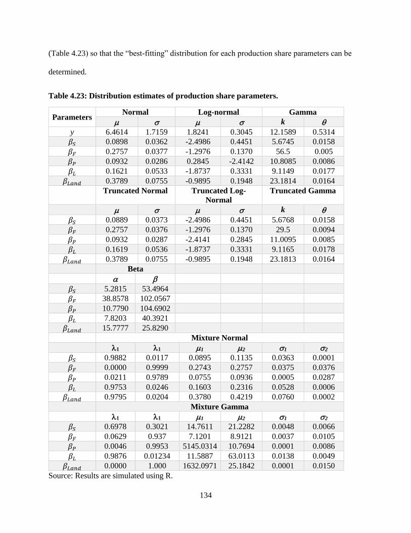
134
(Table 4.23) so that the “best-fitting” distribution for each production share parameters can be
determined.
Table 4.23: Distribution estimates of production share parameters.
Parameters Normal Log-normal Gamma
k
y 6.4614 1.7159 1.8241 0.3045 12.1589 0.5314
𝛽𝑆 0.0898 0.0362 -2.4986 0.4451 5.6745 0.0158
𝛽𝐹 0.2757 0.0377 -1.2976 0.1370 56.5 0.005
𝛽𝑃 0.0932 0.0286 0.2845 -2.4142 10.8085 0.0086
𝛽𝐿 0.1621 0.0533 -1.8737 0.3331 9.1149 0.0177
𝛽𝐿𝑎𝑛𝑑 0.3789 0.0755 -0.9895 0.1948 23.1814 0.0164
Truncated Normal Truncated Log-
Normal
Truncated Gamma
k
𝛽𝑆 0.0889 0.0373 -2.4986 0.4451 5.6768 0.0158
𝛽𝐹 0.2757 0.0376 -1.2976 0.1370 29.5 0.0094
𝛽𝑃 0.0932 0.0287 -2.4141 0.2845 11.0095 0.0085
𝛽𝐿 0.1619 0.0536 -1.8737 0.3331 9.1165 0.0178
𝛽𝐿𝑎𝑛𝑑 0.3789 0.0755 -0.9895 0.1948 23.1813 0.0164
Beta
𝛽𝑆 5.2815 53.4964
𝛽𝐹 38.8578 102.0567
𝛽𝑃 10.7790 104.6902
𝛽𝐿 7.8203 40.3921
𝛽𝐿𝑎𝑛𝑑 15.7777 25.8290
Mixture Normal
1 1 1 2 1 2
𝛽𝑆 0.9882 0.0117 0.0895 0.1135 0.0363 0.0001
𝛽𝐹 0.0000 0.9999 0.2743 0.2757 0.0375 0.0376
𝛽𝑃 0.0211 0.9789 0.0755 0.0936 0.0005 0.0287
𝛽𝐿 0.9753 0.0246 0.1603 0.2316 0.0528 0.0006
𝛽𝐿𝑎𝑛𝑑 0.9795 0.0204 0.3780 0.4219 0.0760 0.0002
Mixture Gamma
1 1 1 2 1 2
𝛽𝑆 0.6978 0.3021 14.7611 21.2282 0.0048 0.0066
𝛽𝐹 0.0629 0.937 7.1201 8.9121 0.0037 0.0105
𝛽𝑃 0.0046 0.9953 5145.0314 10.7694 0.0001 0.0086
𝛽𝐿 0.9876 0.01234 11.5887 63.0113 0.0138 0.0049
𝛽𝐿𝑎𝑛𝑑 0.0000 1.000 1632.0971 25.1842 0.0001 0.0150
Source: Results are simulated using R.

135
Similar to the utility share parameters, the two distributions with lowest AICs are selected
for each production share parameter. For 𝛽𝑆 the mixture Beta and Beta, for 𝛽𝐹 the Beta and Log-
Normal, for 𝛽𝑃 the mixture Beta and Log-Normal, and for 𝛽𝐿 Log-Normal and Gamma
distributions have the lowest AIC and are selected for the analysis (see Table 4.24).
Table 4.24: Results of AIC coefficients for production share parameters.
𝜷𝑺 𝜷𝑭 𝜷𝑷 𝜷𝑳
Distribution
AIC
Distribution
AIC
Distribution
AIC
Distribution
AIC
Mixture
Beta
-467.9297 Beta -443.8854 Mixture
Beta
-541.612 Truncated
Log-Normal
-368.9981
Beta
-458.9038 Log-Normal -443.8471 Log-Normal -536.5031 Log-Normal -368.9981
Truncated
Gamma
-458.2715 Truncated
Log-Normal
-443.8471 Truncated
Log-Normal
-536.5031 Truncated
Gamma
-368.9339
Gamma -458.2699 Normal -442.494 Truncated
Gamma
-529.2981 Gamma -368.9334
Truncated
Normal
-453.3346 Truncated
Normal
-442.494 Gamma -529.119 Beta -368.4992
Normal -451.5359 Gamma -439.7351 Beta -528.1057 Truncated
Normal
-359.2013
Truncated
Log-Normal
-449.3757 Mixture Beta -435.8854 Mixture
Gamma
-521.1742 Normal -358.9058
Log-Normal -449.3757 Mixture
Gamma
-434.6736 Truncated
Normal
-508.531
Mixture
Normal
-445.5912 Mixture
Normal
-434.494 Normal -508.3945
Mixture
Gamma
-431.3286 Truncated
Gamma
-425.9884 Mixture
Normal
-502.1872
Source: Results are simulated using R.
Figure 4.16 provides the graphical analysis for 𝛽𝑆. Based on this figure, the mixture Beta
distribution (blue curve) accurately fits the histogram, which is consistent with the AIC analysis.
Therefore, the mixture Beta is selected over the Beta (red curve) for the seed expenditure share
parameter.
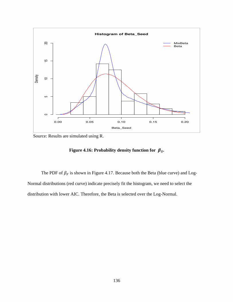
136
Source: Results are simulated using R.
Figure 4.16: Probability density function for 𝜷𝑺.
The PDF of 𝛽𝐹 is shown in Figure 4.17. Because both the Beta (blue curve) and Log-
Normal distributions (red curve) indicate precisely fit the histogram, we need to select the
distribution with lower AIC. Therefore, the Beta is selected over the Log-Normal.

137
Source: Results are simulated using R.
Figure 4.17: Probability density function for 𝜷𝑭.
Figure 4.18 displays the PDFs of 𝛽𝑃, pesticides share parameter. The graphical analysis
indicates the mixture Beta distribution (blue curve) accurately fits the histogram which is
consistent with the AIC results. Therefore, the Mixture Beta is selected over the Log-Normal
distribution (red curve).
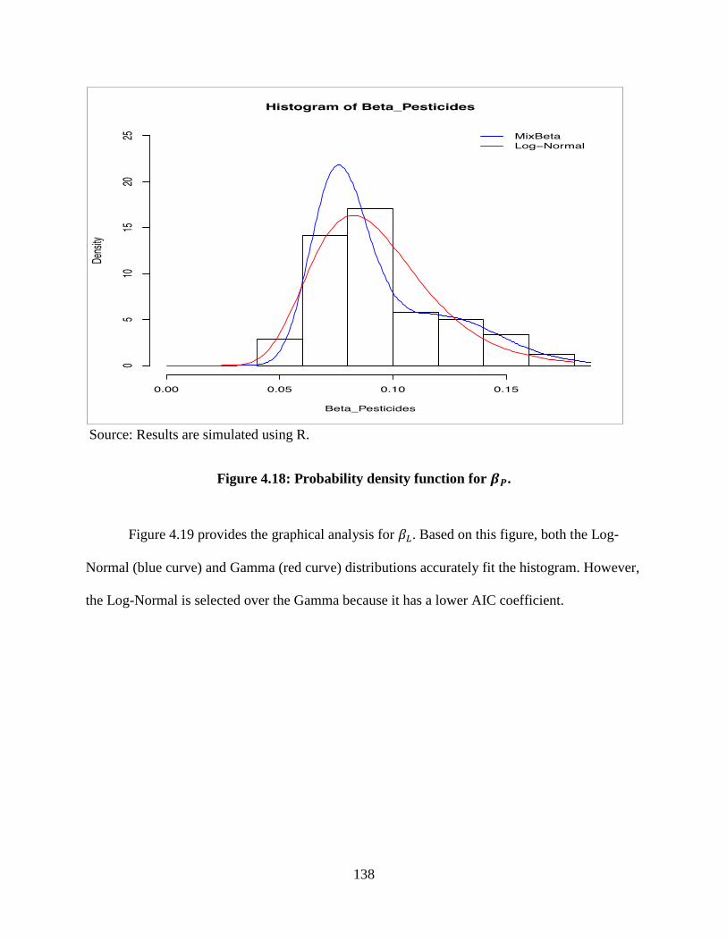
138
Source: Results are simulated using R.
Figure 4.18: Probability density function for 𝜷𝑷.
Figure 4.19 provides the graphical analysis for 𝛽𝐿. Based on this figure, both the Log-
Normal (blue curve) and Gamma (red curve) distributions accurately fit the histogram. However,
the Log-Normal is selected over the Gamma because it has a lower AIC coefficient.

139
Source: Results are simulated using R.
Figure 4.19: Probability density function for 𝜷𝑳.
Since drawing from individual distributions leads to uncorrelated draws, a multi-variate
simulation approach is applied to obtain the correlated draws that accurately represent the
correlation among variables in the three surveys. The Phoon, Quek, and Huang (PQH) (Phoon et
al, 2004) algorithm is applied, which leads to random draws from univariate distributions
mimicking random draws from multivariate distribution. The PQH method provides a very
flexible simulation approach for correlated parameters and describes a procedure for simulating
correlated variables from mixed marginal distributions based on eigen decomposition of the rank
correlation matrix (Anderson, Harri, and Coble, 2009; Phoon, Quek, and Huang, 2002). The

140
PQH algorithm was followed to generate 1,000 correlated random draws for individual farmer
yields (𝑦𝑖s), production share parameters (𝛽𝑖s), and consumption share parameters (𝛼𝑗s).
The correlation coefficients of utility and production parameters that present in Table 4.25 and
4.26 confirm each parameter is correlated.
Table 4.25: Correlation coefficients of utility share parameters.
Utility Parameters 𝜶𝒓 𝜶𝒂 𝜶𝒎
𝛼𝑟 1.0000 0.2902 -0.4679
𝛼𝑎 0.2902 1.0000 -0.9815
𝛼𝑚 -0.4679 -0.9815 1.0000
Source: Results are simulated using R.
Table 4.26: Correlation coefficients of production share parameters.
Production Parameters 𝜷𝑺 𝜷𝑭 𝜷𝑷 𝜷𝑳
𝛽𝑆 1.0000 -0.1996 -0.0176 -0.1649
𝛽𝐹 -0.1996 1.0000 0.1090 0.0882
𝛽𝑃 -0.0176 0.1090 1.0000 -0.0212
𝛽𝐿 -0.1649 0.0882 -0.0212 1.0000
Source: Results are simulated using R.
3.3 Model Calibration
With correlated random draws for individual farmer yields (𝑦𝑖s) and production (𝛽𝑖s) and
consumption (𝛼𝑖s) share parameters from selected distribution estimates, the next step is to
define and calibrate the remaining parameters in the model. Both the producer price of long-
grain paddy rice and the consumer price of long-grain milled rice are obtained from RICEFLOW
model. Other data such as minimum wage, average farm size, input prices (price of seed,
fertilizer, pesticides), average of household members, total available hours in a year (average
number of people times 24 hours in a day multiplies by 365 days in a year) are obtained from
household surveys.

141
Given the correlated random draws for 𝛽𝑖s and 𝑦𝑖s, prices of long-grain paddy rice and
inputs, and analytical solution for input demand functions equations [31] – [34], the productivity
parameter 𝐴 is calibrated as a residual: 𝐴𝑖 =𝑦𝑖
𝑥𝑆𝑖 (∙)𝛽𝑆
𝑖 𝑥𝐹
𝑖 (∙)𝛽𝐹𝑖
𝑥𝑃𝑖 (∙)𝛽𝑃
𝑖𝑥𝐿
𝑖 (∙)𝛽𝐿𝑖 . The RICEFLOW analysis
generates baseline results for the year 2020, and predicts domestic production will increase by
6.8% by 2020. Consequently, productivity parameter is increased by 6.856% over the calibrated
values to match this rise in production. Therefore, the baseline year in RICEFLOW and the
baseline year in the current study are consistent.
With the production parameters calibrated, government transfer 𝑇 is calibrated such that
income from rice production matches the current income-based poverty rates among rice farmers
to 16.82% (HIS, 2016). The CES parameter 𝜌 between rice, manufacturing, and leisure is
assumed to be -2, which implies an elasticity of substitution 𝜎 =1
1−𝜌 of 0.33 and the
consumption goods are imperfectly substitutable34. With total expenditures on rice and
composite non-rice consumption reported in HIS (2016), distributions of the expenditure share of
these consumable goods are estimated in the preceding subsection 3.2.2 Distribution Estimation
of Utility Share Parameters. However, data on the value of leisure (and thus expenditure share
𝛼𝐿𝑖 ) or the consumer price of the composite non-rice good �̃�𝑀 does not exist. Therefore,
assuming a common leisure share parameter among all households (𝛼𝐿𝑖 = 𝛼𝐿), 𝛼𝐿 and �̃�𝑀 are
calibrated to match two facts: the average household spends 72% (HIS, 2016) of their time at
leisure and consumes 88.9 kg/person of rice per year (MARDI, 2014). With 𝛼𝐿 and �̃�𝑀
34 The estimation and assumption of CES parameter 𝜌 can be referred to Constant Elasticity
Functions (Rutherford, 2002).

142
parameterized, all exogenous variables are defined, and the model can be simulated to quantify
the effects of free trade on farm households.
4. Empirical Results and Discussions
With the prices and exogenous parameters defined in the Data and Model Calibration
section 3, equations [30] – [37] are simulated for the empirical analysis. The simulation analysis
is run for each of the 1,000 individual farmers randomly drawn using the estimated univariate
distributions and the PQH algorithm. Two scenarios are run for each farmer to quantify the
effects of free trade policy: First, in the baseline scenario, all prices are maintained at the levels
specified in the calibration, which results in the model closely reproducing the survey data for
input demands, production, income, and farmers’ demand for rice, composite non-rice, and
leisure. Second, in the alternate scenario, the effects of free trade in the Malaysian rice sector
from the RICEFLOW analysis on the producer price of long-grain paddy rice (𝑝𝑅) and consumer
price of long-grain white rice ( �̃�𝑅) are imposed on the system of equations. Specifically, 𝑝𝑅 is
decreased by 11.9% and �̃�𝑅 is reduced by 14.74%, as reported in the free-trade scenario in
Chapter 3. The solutions of the baseline and alternate scenarios are then used to calculate the
poverty and welfare measures for both scenarios. Finally, the solutions of the endogenous
variables, poverty, and welfare measures in the baseline and alternate scenarios are compared to
quantify the effects of free trade in the Malaysian rice sector on rice farmers.
4.1 Production
The impacts of free trade policy on rice production are quantified as the percent change
in inputs and rice yield from the baseline to the alternate scenario for each rice farmer. The

143
income is then computed for each farmer and compared to the poverty level to find the
proportion of farmers that are poor under both scenarios.
4.1.1 Production Impact
The decline in producer price for long-grain paddy rice after the implementation of free
trade, results in the factors of production (seeds, fertilizers, pesticides, and labor) decreasing on
average by 16.16% with standard deviations of 0.77, which indicates the varied effect of the free
trade policy among the rice farmers. While the Cobb-Douglas structure of the production
function results in the same percentage decline in inputs, the absolute differences in input use
vary. From the baseline, seed, fertilizer, pesticide, and total labor per hectare decline to a level of
198.68 kg, 4.76 kg, 27.88 liters, and 22.10 hours, respectively. The reduction of inputs leads to a
decline in rice yield by 4.84%, from 6.96 Mt/Ha to 6.62 Mt/Ha. However, the estimated yields
effect is divergent between rice farms as the standard deviation of the percent change is 0.88
(Table 4.27). Hence, these results show that rice farmer’s production declines from the free trade
policy, which is consistent with the trade theory of a small country effect.
Table 4.27: The impacts of free trade policy on domestic production.
Source: Results are simulated using R.
Parameters
Baseline 2020
Free Trade Policy Scenario
Level % Change (Std. Dev.)
Seed (Kg) 236.98 198.68 -16.16 (0.77)
Fertilizer (Kg) 5.68 4.76 -16.16 (0.77)
Pesticide (Liter) 33.25 27.88 -16.16 (0.77)
Labor (Hrs) 26.36 22.10 -16.16 (0.77)
Yield (Mt/Ha) 6.96 6.62 -4.84 (0.88)

144
4.1.2 Income Poverty Measure
The significant decrease in production inputs and rice yield leads to a decline in domestic
production after the implementation of free trade. This causes rice farmers’ household income to
fall relative to the baseline. As a result, the percent of rice farmers who generate monthly
household income below RM 800 (the average national poverty line for poor) increased from
16.40% to 33.20%, while those earning below RM 460 (the average national poverty line for
extreme poor) surged from 11.30% to 22.30% (Table 4.28). Because free trade leads to more rice
imports, the international competition for domestic rice farmers is stronger. Thus, for the rice
farmers, free trade will negatively affect incomes leading to escalating poverty rates of both poor
and extreme poor. However, while the farm gate price of rice and production falls, leading to
lower income, the consumer price of rice also declines. While rice farmers experience a negative
income shock, they could actually consume more of the staple food with a lower consumer price
for rice.
Table 4.28: Income poverty measures for baseline and free trade.
Parameters Baseline (%) Free Trade (%)
Monthly household income < RM 800 16.40 33.20
Monthly household income < RM 460 11.30 22.30
Source: Results are simulated using R.
4.2 Consumption
The impacts of free trade policy on households’ consumption are measured as the percent
change in the average per capita rice consumption, non-rice consumption, and leisure hours,
from the baseline to the alternate scenario for each household. The rice consumption is then
145
computed for each household and compared to the poverty level to find the proportion of
households that are below the subsistence level of rice consumption per person under both
scenarios.
4.2.1 Consumer Demand Effect
The decrease in consumer price for long grain rice after free trade implementation leads
to an increase in rice consumption by 5.01% on average with a standard deviation of 0.11. The
consumption increases from 533.40 to 560.12 Kg per household of six (or 88.9 per person) from
the baseline to the alternate scenario level, respectively. Since rice becomes more affordable due
to the lower market rice prices, consumers have higher purchasing power after free trade
implementation. Both composite non-rice consumption and leisure (non-working hours) decline
slightly by 0.42%. These results indicate that farmers reduce consumption of composite non-rice,
but extend family working hours on the rice farm, which partially offsets the reduction in
income.35 From the baseline, composite non-rice consumption and leisure decrease to a level of
147.91 and 37,736.60, respectively (Table 4.29). On the consumption side, the results suggest
that rice farmers are better off with the implementation of free trade. With affordability as a key
pillar of food-security, free trade plays a significant role in Malaysia’s food security as it leads to
a lower price and more rice consumption.
35 If total working hours are falling while family working hours are rising, then hired labor hours
on the farm must be declining.

146
Table 4.29: The impacts of free trade on farm household consumption
(per household per year).
Parameters Baseline 2020 Free Trade Policy Scenario
% Change Level (Std. Dev.)
Rice consumption (Kg)
533.40
5.01
560.12 (0.11)
Composite non-rice
Consumption index
148.53
-0.42
147.91 (0.10)
Leisure (Hr)
37,895.76
-0.42
37,736.60 (0.10)
Source: Results are simulated using R.
4.2.2 Rice Consumption Poverty Measure
The rice consumption poverty line is measured at 70 Kg per person (i.e. the minimum
rice consumption per Kg per year from HIES). Free trade results in the proportion of farmers
below 70 Kg per person to decline from 18.40% in baseline to 14.10% after the implementation
of free trade. This suggests that poverty—measured in terms of rice consumption—will be
alleviated for rice farmers when free trade is allowed.
4.3 Farmers’ Welfare Measure
With the income and rice consumption poverty measures leading to opposing conclusions
about the poverty of rice farmers, a comprehensive welfare analysis for rice farmers is conducted
by calculating equivalent variations for each household before and after free trade. This welfare
measure is more comprehensive than the poverty estimates because it accounts for both income
and price effects simultaneously. Note that the equivalent measure is for rice farm households
only and is not a national welfare measure of free trade. After the implementation of the free
trade policy, the index of equivalent variation welfare measure for farm households declines
marginally by -0.42 from the baseline. Since the decrease is very marginal, less than one, the

147
results suggest that free trade causes no significant impact on individual farmers’ income and
welfare.
From a policy perspective, free trade will lead to a substantial increase in consumer
surplus in rice consumption—not just for rice farmers but for all Malaysian rice consumers.
Therefore, opening the rice market to free trade, while providing compensation to rice farmers to
alleviate the negative impacts of free trade, could still be welfare improving for Malaysia as a
whole. While free trade hurts rice farmers in terms of income and equivalent variation, there are
policy combinations that can allow for free trade while leaving farmers equally well off.
5. Conclusions
Poverty alleviation, especially for rural rice farmers, has been a long-standing goal in
Malaysian national rice policy, as reflected in the government’s efforts to embark on various
support and protective policies to enhance farmers’ livelihoods and welfare. One of the key trade
policies that has been in place for decades is large tariffs on rice imports. In fact, the most recent
policy review suggests prohibitive barriers in rice trades to pursue an autarky rice economy.
Despite having participated in both bilateral and regional free trade agreements (FTA), Malaysia
excluded rice from the FTAs since it is classified as a sensitive commodity.
This study analyzes the impact including rice in the FTAs would have on rice farmers by
developing a farm household model for individual rice farmers in Malaysia. The model is
simulated to evaluate the impacts of free trade—through changes in producer and consumer
prices from the RICEFLOW analysis in Chapter 3—on rice farmers’ production, consumption,
poverty, and welfare. The results indicate that even though free trade would hurt rice farmers in
Malaysia due to increasing the percentage of farmers’ living below the national poverty line,
farmers would increase their rice consumption due to the lower rice prices after the free trade,

148
which also benefits non-farm rice consumers in Malaysia. However, the equivalent variation (a
complete welfare measure that combines both the effects of income and rice consumption) shows
that free trade does make rice farmers worse off as their welfare falls, albeit minimally. While
rice farmers are highly protected in Malaysia, the impacts of free trade are often misconstrued to
focus only on the negative effects on the domestic production side and rice farmers’ incomes and
welfare. This study provides key insights on the economic assessment of moving to a more
liberalized rice market to the Malaysian government and policy makers.
The welfare measures from this study focuses on rice farmers, and thus the results do not
represent the entire rice consumer’s population and the whole economy. Given the negative
welfare effect, an important extension of this analysis will modify the model to study the most
efficient government transfer to make farmers equally well off, while still allowing for free trade.
Specifically, this extension could evaluate whether bolstering current production subsidies or
shifting to decoupled direct payments would be the most cost-effective policy.

149
References
Alam, M., Siwar, C., Murad, M.W., Molla, R.I., and Toriman, M.E. (2010). Socioeconomic
Profile of Farmer in Malaysia: Study on Integrated Agricultural Development Area in
North-West Selangor. Agricultural Economics and Rural Development, vol. VII:2, pp.
249–265.
Burkardt, J. (2014). The Truncated Normal Distribution. Department of Scientific Computing,
Florida States University.
De Janvry, A., and Sadoulet, E. (2016). Progress in The Modeling of Rural Households'
Behavior Under Market Failures in Poverty, Inequality and Development. Kluwer
Publishing.
De Janvry, A., Fafchamps, M., and Sadoulet, E. (1991). Peasant Household Behavior with
Missing Markets: Some Paradoxes Explained. The Economic Journal, Vol. 101:409, pp.
1400 – 1417.
Fahmi, Z., Abu Samah, B., and Abdullah, H. (2013). Paddy Industry and Paddy Farmers Well-
being: A Success Recipe for Agriculture Industry in Malaysia. Asian Social Science; Vol.
9: ISSN 1911-2017, E-ISSN 1911-2025. Canadian Center of Science and Education.
Food and Agricultural Policy Research Institute. (2007). U.S and World Agricultural Outlook.
FAPRI Staff Report 07-FSR 1. ISSN 1534-4533.
Fujimoto, A. (1996). Rice Land Ownership and Tenancy Systems in Southeast Asia: Facts and
Issues Based on Ten Village Studies. The Developing Economies, XXXIV-3, September
1996. Retrieved from onlinelibrary.wiley.com.
International Rice Research Institute. (1985). Impact of Science on Rice. IRRI, Manila,
Philippines. ISBN: 971-104-144-8.
Ishida, A., Law, S.H., and Aita, Y. (2003). Changes in food consumption expenditure in
Malaysia. Agribusiness, 19: 61–76. doi:10.1002/agr.10038.
Malaysian Agricultural Research and Development Institute. (2013). Survey on Household
Income and Expenditure on Rice Farmers in Malaysia.
150
Meyer, B. D., and Sullivan, J.X. (2012). Identifying the Disadvantaged: Official Poverty,
Consumption Poverty, and the New Supplemental Poverty Measure. Journal of Economic
Perspectives, Vol. 26:3, pp. 111-36.
Meyer, B. D., and Sullivan, J.X. (2011). Viewpoint: Further Results on Measuring the Well-
Being of the Poor Using Income and Consumption. Canadian Journal of Economics
44(1): 52–87.
Meyer, B. D., and Sullivan, J.X. (2003). Measuring the Well-Being of the Poor Using Income
and Consumption. Journal of Human Resources 38(S): 1180–1220.
Phoon, K., S. T. Quek, and H. Huang. 2004. Simulation of Non-Gaussian Processes Using
Fractile Correlation. Probabilistic Engineering Mechanics. 19: 287-292.
Singh, I., Squire, L., and Strauss, J. (1986). Agricultural Household Models: Extension,
Applications, and Policy. Published for the World Bank.
Rabu, M.R., and Mohd Shah, M.D. (2013). Food and Livelihood Security of the Malaysian
Paddy farmers. Economic and Technology Management Review, vol. 8, pp. 69 – 79.
Rutherford, T. F. 2002. Lecture Notes on Constant Elasticity Function. University of Colorado.
Siwar, C., Yasar, M., Ghazali, R., and Mohd Idris, N. (2013). Vulnerability and Sustainable
Livelihood of Paddy Farmers in The North Terengganu Integrated Agriculture
Development Area (IADA KETARA), Malaysia. Proceedings PERKEM VIII: 2, 778 –
789. ISSN:2231-962X.
Taylor, J. E., and Adelman, I. (2002). Agricultural Household Model: Genesis, Evolution, and
Extensions. Review of Economics of the Household, vol.1:1. University of California,
Davis, CA.
Tey, Y.S., Shamsudin, M.N., Mohamed, Z., Abdullah, A.M. (2009). Demand Analysis of Food
in Malaysia: A Study of Malay Ethnic. Online at http://mpra.ub.uni-muenchen.de/15064/
MPRA Paper No. 15064.

151
Thorbecke, E. (1993). “Impact of State and Civil Institutions on the Operation of Rural Markets
and Nonmarket Configurations.” World Development, 21(4): 591-605.
World Bank. (2012). Rice Irrigation in Malaysia: Economic Change and the Choice of Irrigation
Technology.
Yotopoulos, P., and Lawrence J. L. (1974). “On Modeling the Agricultural Sector in Developing
Economies: An Integrated Approach of Micro and Macroeconomics, Journal of
Development Economics, 1(2): 105-127.

152
Appendix 4.1: The simplification of utility functions.
�̃�𝑅𝑐𝑅 + 𝑝𝑀𝑐𝑀 ≤ 𝑝𝑅𝐹𝑅 (𝑥𝑆, 𝑥𝐹 , 𝑥𝑃, 𝑥𝐿) − 𝑟𝑆𝑥𝑆 − 𝑟𝐹𝑥𝐹 − 𝑟𝑃𝑥𝑃 − 𝑟𝐿(𝑥𝐿 − 𝑡̅ + 𝑐𝐿)) − 𝑇
�̃�𝑅𝑐𝑅 + 𝑝𝑀𝑐𝑀 ≤ 𝑝𝑅𝐹𝑅 (𝑥𝑆, 𝑥𝐹 , 𝑥𝑃, 𝑥𝐿) − 𝑟𝑆𝑥𝑆 − 𝑟𝐹𝑥𝐹 − 𝑟𝑃𝑥𝑃 − 𝑟𝐿𝑥𝐿 + 𝑟𝐿𝑡̅ − 𝑟𝐿𝑐𝐿 − 𝑇
�̃�𝑅𝑐𝑅 + 𝑝𝑀𝑐𝑀 + 𝑟𝐿𝑐𝐿 ≤ 𝑟𝐿𝑡̅ + 𝑝𝑅𝐹𝑅 (𝑥𝑆, 𝑥𝐹 , 𝑥𝑃, 𝑥𝐿) − 𝑟𝑆𝑥𝑆 − 𝑟𝐹𝑥𝐹 − 𝑟𝑃𝑥𝑃 − 𝑟𝐿𝑥𝐿

153
Appendix 4.2: The first order conditions (FOCs) of eliminating 𝝀.
𝜕ℒ
𝜕𝑐𝑅=
𝛼𝐶𝛼𝑅𝑐𝑅𝛼𝑅−1
𝑐𝑀𝛼𝑀(𝑐𝐶
𝛼𝐶 𝑐𝑀𝛼𝑀)𝛼𝐶−1 𝑐𝐿
𝛼𝐿
𝛼𝐿(𝑐𝑅𝛼𝑅 𝑐𝑀
𝛼𝑀)𝛼𝐶 𝑐𝐿𝛼𝐿−1
− 𝜆 �̃�𝑅
𝜆𝑟𝐿= 0
𝜕ℒ
𝜕𝑐𝑀=
𝛼𝐶𝛼𝑀𝑐𝑅𝛼𝑅
𝑐𝑀𝛼𝑀−1
(𝑐𝑅𝛼𝑅 𝑐𝑀
𝛼𝑀)𝛼𝐶−1 𝑐𝐿𝛼𝐿
𝛼𝐿(𝑐𝑅𝛼𝑅 𝑐𝑀
𝛼𝑀)𝛼𝐶 𝑐𝐿𝛼𝐿−1
− 𝜆𝑝𝑀
𝜆𝑟𝐿= 0
𝜕ℒ
𝜕𝑐𝐿= 𝛼𝐿 (𝑐𝑅
𝛼𝑅 𝑐𝑀𝛼𝑀)𝛼𝐶 𝑐𝐿
𝛼𝐿−1− 𝜆𝑟𝐿 = 0
𝜕ℒ
𝜕𝑥𝑆= 𝑝𝑅 𝛽𝑆 𝐴𝑥𝑆
𝛽𝑆−1 𝑥𝐹
𝛽𝐹 𝑥𝑃𝛽𝑃 𝑥𝐿
𝛽𝐿 − 𝑟𝑆 = 0
𝜕ℒ
𝜕𝑥𝐹= 𝑝𝑅 𝛽𝐹 𝐴𝑥𝑆
𝛽𝑆 𝑥𝐹𝛽𝐹−1
𝑥𝑃𝛽𝑃 𝑥𝐿
𝛽𝐿 − 𝑟𝐹 = 0
𝜕ℒ
𝜕𝑥𝑃= 𝑝𝑅 𝛽𝑃 𝐴𝑥𝑆
𝛽𝑆 𝑥𝐹𝛽𝐹 𝑥𝑃
𝛽𝑃−1 𝑥𝐿
𝛽𝐿 − 𝑟𝑃 = 0
𝜕ℒ
𝜕𝑥𝐿= 𝑝𝑅 𝛽𝑃 𝐴𝑥𝑆
𝛽𝑆 𝑥𝐹𝛽𝐹 𝑥𝑃
𝛽𝑃 𝑥𝐿𝛽𝐿−1
− 𝑟𝐿 = 0
𝜕ℒ
𝜕𝜆= ( 𝑟𝐿𝑡̅ + 𝑝𝑅 𝐴𝑥𝑆
𝛽𝑆 𝑥𝐹𝛽𝐹 𝑥𝑃
𝛽𝑃 𝑥𝐿𝛽𝐿 − 𝑟𝑆𝑥𝑆 − 𝑟𝐹𝑥𝐹 − 𝑟𝑃𝑥𝑃 − 𝑟𝐿𝑥𝐿 − ( �̃�𝑅𝑐𝑅 + 𝑝𝑀𝑐𝑀 + 𝑟𝐿𝑐𝐿)
− 𝑇 = 0
154
Chapter V
Economic Insights into Malaysian Rice Policy: Concluding Remarks
1. Dissertation Summary
This dissertation research demonstrates the integration of agricultural economics and
public policy to comprehensively evaluate and analyze a deep-rooted rice policy in Malaysia,
primarily the impact of self-sufficiency and international trade policies at both the macro and
micro levels. It consists of three sequential empirical studies using different quantitative
methodologies that applies economic frameworks as the major mode of analysis. The fact that
the Malaysia’s rice policy is a strategy of achieving self-sufficiency while the status quo of the
national rice economy remains ambiguous, motivates this research to initially measure the
competitiveness and comparative advantage of the domestic rice production and analyze the
efficiency policies at the farm level. Therefore, prior to the major evaluation and analysis on self-
sufficiency and international free trade policies, we determine the current efficiency of domestic
rice production with the self-sufficiency policy emphasis and provide foundational evidences on
the current situation of policy consequences at the farm level. Further, the major analysis
evaluates the impact of self-sufficiency and international trade policies on the rice sector at the
national level in light of food security concerns. Finally, the study presents deeper evaluation and
analyzes the impacts of the international trade policy at the farm-household level, on the
heterogeneous rice farmers in Malaysia. While limited studies have attempted to analyze the
Malaysian rice policies, these empirical studies establish the crucial rice policy concerns in
Malaysia; self-sufficiency, international free trade, and food security. The specific research
encompasses: 1) measuring the competitiveness and efficiency of rice production policy using a
Policy Analysis Matrix, 2) evaluation and impact of self-sufficiency and international free trade

155
policies using a RICEFLOW model, and 3) evaluation and impact of international free trade on
rice farmers using a Farm-Household model. The results of these studies also address food
security concerns.
1.1 The Competitiveness and Efficiency of Rice Production
This study evaluates and analyzes domestic rice production system at farm level in
Malaysia since the competitiveness and comparative advantage of domestic rice production has
been distorted through high levels of intervention, protection, and subsidy supports provided by
the government for many years. A wide range of policy programs have been implemented, most
of which include input and output subsidies and regulated producer price with the goal being to
achieve total self-sufficiency in rice. Even though the rice sector contributes a relatively small
share to the national income, rice still receives special attention and has been given priority in a
series of the national development policies in Malaysia. While subsidies have become a
permanent policy strategy for decades and have involved substantial public investment, the
domestic rice outcomes remain stagnant and only satisfy between 60-65% of the growing
demand each year. In fact, the recent revised national rice policy provides more additional input
and output subsidies which will continue to burden government expenditure. Recently, the
government decided to more seriously pursue self-sufficiency, aiming to eliminate all rice
imports in the future.
This study applies policy analysis matrix approach to measure the competitiveness and
comparative advantage of the domestic rice production system in Malaysia. The results indicate
that while receiving substantial efforts and attention by the government, especially through
realizing various production support programs, domestic rice is still lacking comparative
advantage relative to rice imports. Currently, the total rice production subsidy is RM 2,571.3 (per

156
hectare) which accounts 59.1% of the total production cost (per hectare). With these substantial
subsidies and producer price support, the average farmers’ net income is significantly low, RM
703.36 (per hectare), which is below the national poverty line, RM 800 per household of six. If
all subsidies and price support are removed, rice farmers would suffer from significant losses
(RM 2,984.33 per hectare) due to high production costs for rice at the farm level.
In addition, the protection measures also imply that the current policies are reducing the
actual input costs while increasing the revenue through subsidizing inputs and imposing higher
domestic prices than world market prices. The divergence is caused by the government policies
that distort the pattern of production, moving it away from the most efficient use of domestic
resources and international trading opportunities. The competitiveness analysis verifies that the
government decision in pursuing self-sufficiency through highly protecting the domestic rice
industry leads to significant policy distortion since the international rice price is lower than
domestic rice. This study provides foundational information that domestic rice production in
Malaysia is not competitive since the protectionist policies have failed to achieve self-
sufficiency.
1.2 The Impact of Self-sufficiency and International Trade
Self-sufficiency, often misinterpreted as food security, has become a permanent policy
goal in the national rice development plan in Malaysia. This primarily concerns addressing the
national food security over the past decades. The government’s mandate under the national agro-
food policy, 2010-2020, is to pursue self-sufficiency in rice and achieve total self-sufficiency by
the year 2020. With this mandate, the government aims to close all trading borders and eliminate
rice imports coming from international markets and suppliers. As Malaysia is not a competitive
rice producer, this extreme policy decision would lead to massive additional expenditures at the

157
production and farm levels. This study evaluates and analyzes the impact of self-sufficiency
policy in rice at the national level using the RICEFLOW model.
A self-sufficiency policy scenario is defined as the removal of rice imports for long grain
rice by the year 2020. With elimination of rice imports, domestic rice production would increase
as well as the producer price. This increase also implies the increase in cost of production that is
mostly derived from a constraint in land factor. The higher production cost of paddy rice and
consequential increase in the market price of paddy rice transfers to higher consumer prices. As
a result, the domestic demand for consumption of long grain rice declines. These results imply
that self-sufficiency improve rice producers’ welfare which would benefit them, however the
policy punishes all rice consumers, which also include the rice producer as consumer, due to a
substantial increase in consumer price. Hence, rice self-sufficiency entails significant welfare
shifts from consumers to producers and will likely adversely affect food security objectives since
the policy increases prices and limits consumption, especially by the poor. As affordable food
prices are the key pillars of food security, self-sufficiency does not guarantee food security at the
national level. The government would suffer from losses of the import tariff revenues. In
addition, self-sufficiency burdens the government with substantial additional expenditure for the
required output subsidies, production inputs, and technological efficiency to realize self-
sufficiency in rice while maintaining consumer prices.
In contrast, liberalizing rice trade, which has been found to provide positive effects on
food security, would be an alternative policy strategy, since Malaysia is a member of ASEAN,
WTO, and has actively participated in both bilateral and regional free trade agreements for other
commodities. With free trade, although rice producers are worse off, albeit to a marginal degree,
and though the government loses from import tariff revenues, consumers would be better off due

158
to decreasing prices with a more competitive market environment from external rice suppliers. In
addition, Malaysia could participate in a regional approach for strengthening food security to
address its rice-deficit issue, and thus free trade could offer a more food secure economy. The
results of these two policy scenarios correspond to economic theory that self-sufficiency greatly
benefits rice farmers at the expense of consumers. On the other hand, the free trade showed
opposite policy impacts since farmers’ welfare worsens, yet consumers’ welfare increases. From
this study, these policy scenarios clearly represent the opposite direction in terms of welfare
distribution. Further, the price effects of the free trade policy scenario are applied in the
following study to measure the policy impacts at the household level among rice farmers in
Malaysia.
1.3 The Impact of International Free Trade on Rice Households
While rice farmers are highly protected in Malaysia, the impacts of free trade are often
misconstrued to focus only on the negative effects on the domestic production side and rice
farmers’ incomes and welfare. Therefore, this study analyzes the impact of free trade policy that
would have on rice farmers by developing a farm household model for individual rice farmers in
Malaysia. The model is simulated to evaluate the impacts of free trade—through changes in
producer and consumer prices from the RICEFLOW analysis in Chapter 3—on rice farmers’
production, consumption, poverty, and welfare.
The decline in producer price after the free trade policy reduces the production input use
(seed, fertilizer, pesticide, and total labor) among rice farmers. The significant decrease in
production inputs also causes in decrease rice yield and further leads to decline in domestic
production after the implementation of free trade. These consequences cause rice farmers’

159
household incomes to fall. Because free trade leads to more rice imports, the international
competition for domestic rice farmers is stronger. Thus, for the rice farmers, free trade will
negatively affect incomes leading to escalating poverty rates of both poor and extreme poor.
However, the decrease in consumer price for long grain rice after free trade leads to an increase
in rice consumption. This suggests that poverty—measured in terms of rice consumption—will
be alleviated for rice farmers when free trade is allowed. The decrease in consumer price not
only benefits rice farmers, but also the entire Malaysian consumers. A complete welfare measure
that combines both the effects of income and rice consumption shows that free trade does make
rice farmers worse off as their welfare falls, albeit minimally.
2. Policy Discussions
With the evaluations and analysis on the Malaysian rice policy, we identify crucial
consequences of the protectionist production policy, the self-sufficiency policy, and the
international free trade policy. The impacts of these policies provide key insights for the
government and policy makers for future rice policy direction.
2.1 Protectionist Policy Consequences
The government’s interventionist policy instruments have significantly distorted prices
and resource use and failed to drive competitiveness in the Malaysian rice sector. These
distortions have induced unnecessary efficiency losses in order to realize the national self-
sufficiency goal. The government enacts distorting policies to favor particular interest groups,
consciously trading off the consequent economic efficiency losses against equity concerns for
special interests of rice farmers.

160
The dominant use of power in decision-making by asking how issues are suppressed, hence the
scope of decision-making is restricted (Bachrach and Baratz, 1962). While “Agenda setting is
not just about what issues government chooses to act on, they are also about competing
interpretations of political problems and the alternative worldviews that underlie them” (Cobb
and Ross, 1997). With implementing protectionist policy, the government does not only distort
the rice market, but also each agricultural input market which includes seed, fertilizer, pesticide,
and other chemicals. As rice in Malaysia is mostly operated by small farmers, it would be highly
challenging to become a globally competitive industry and would require significant financial
supports by the government. The government policies should lead to the economic development
at the macro level instead of stimulating policies to largely focus on rice economy. To realize
total national self-sufficiency goal, the rice sector is largely subsidized, protected and regulated
by the government. The policy evaluation and analysis at the production level reveals that if
domestic support policies are removed– input subsidies and producer price – rice would be
unprofitable to produce in Malaysia, hence an uncompetitive industry, which leads to significant
losses at farm level. However, one of the limitations of this study is that the issue of how rice
farming resources would be redirected to other farming activities was not explored. A high
protection by the government causes inefficient rice production due to policy distortions, since
domestic rice production has no comparative advantage relative to rice imports, which can be
purchased by consumers as much lower prices than domestic rice. Therefore, the government’s
interventionist policy instruments significantly distort rice markets while inducing unnecessary
efficiency losses to realize the national self-sufficiency goal.

161
2.2 Self-sufficiency Policy Consequences
Self-sufficiency has been upheld as a policy strategy in the Malaysian rice sector as a
means to address the food security concerns of its population and to alleviate poverty among rice
farmers, as well as their livelihoods and welfare, which have become permanent mandates in the
national rice development policy. Although self-sufficiency is not a new strategy in Malaysian
policy, having originated in the 1930s, the catastrophic effects of the recent global food crisis in
2007/08 has convinced the government to mandate total self-sufficiency in its primary food
staple, rice, by the year 2020, which has been recently extended to 2050 in the National
Transformation (2020-2050), the national masterplan, through closing borders for rice imports in
the future. With Malaysia is not a competitive rice producer and has no comparative advantage
relative to rice imports, self-sufficiency constantly forces domestic production through high
subsidies for inputs, outputs, and producer prices, hence it is not an efficient approach to pursue.
In fact, domestic production is significantly distorted. Self-sufficiency has also been identified as
a costlier and a counterproductive path to food security. Instead to achieve the food security
objective, self-sufficiency could essentially threaten the overall food security of the country.
With the evidence presented in this study, self-sufficiency in rice is more likely to be considered
as a more political strategy rather than a solution to poverty issues. Furthermore, the food self-
sufficiency approach has been widely criticized as containing misguided policy decisions and
seeks to achieve food security that places political priorities over economic efficiency (Clapp,
2017).
While the self-sufficiency policy would benefit and improve welfare to rice producers,
albeit a minor group of the total population, the policy will not only worsen the majority of
Malaysia’s population of rice consumers, but require large government costs, hence burdening
162
the government fiscal resources. The government’s stance on self-sufficiency needs to be
redefined as current policy decisions are misguided. The significant differences in welfare
allocation between the self-sufficiency and free trade strategies described above imply that the
political economy becomes even more crucial to decide the policy output. With the pursuit of
self-sufficiency, the forces supporting a small group (rice farmers) of the population are
“winning” the battle at the expense of the larger consumer group. Self-sufficiency could also be a
political strategy for the country to become an independent region without relying other
countries’ food sources. Also, the policy decision might be connected to government favoritism
of business interest groups. In fact, the policy decision might actually be shielding political
interests over economic rationale. The policy agenda setting is associated with a process of
conflict and most of politics revolve around the development and expansion of conflict
surrounding evolving political issues (Schattschneider, 1960). Subsidy programs that are
supposed to be an economic tool using substantial government expenditure to improve local rice
industry might be misused as an “exchange” for political desires. In fact, members of
government are “single minded seekers of reelection” (Mayhew, 1974).
2.3 International Trade Policy Consequences
The livelihood and welfare of rice farmers have been protected by the government since
the majority of Malaysian rice farmers are among poor households. Other than a wide range of
domestic support policies for rice farmers, the government also imposes high tariffs for rice
imports. In fact, the most recent policy review suggests prohibitive barriers in rice trade to
pursue an autarky rice economy. Both RICEFLOW and Farm-Household models are applied to
evaluate and analyze the international free trade policy impacts at the macro and micro levels,
respectively. The results indicate consistent impacts at both levels that the international free trade

163
policy reduces producer prices, albeit at different magnitudes. At the national level, the producer
price decreases by 11.9%, and even more at the household level, where it decreases by 16.2%.
The reduction of producer price at the farm-household level causes in reduction of production
inputs – seed, fertilizer, pesticide, and total labor – which decreases long grain rice yield by
4.84%, from 6.96 to 6.62 metric ton per hectare. As a result, the domestic rice production falls by
5.3%.
These free trade consequences further lead to a higher poverty rate of income among rice
farmers in Malaysia. The poverty rate of farmers who generate monthly household income below
RM 800 (the national poverty line for poor) increased from 16.40% to 33.20%, while those
earning below RM 460 (the national poverty line for extreme poor) surged from 11.30% to
22.30%. Because free trade encourages more rice imports by 19.85%, the international
competition facing local rice farmers would be much stronger. On the other hand, free trade
reduces consumer prices of long grain rice by 14.7% which leads to higher growth of rice
consumption by 4.4% at the national level and 5.01% at the farm-household level. Thus, the
poverty rate of rice consumption (farmers who consume below 70 Kg per person/year) declines
from 18.4% to 14.1% after allowing free trade.
While rice farmers experience a negative income shock, they actually consume more of
the staple food with a lower consumer price for rice. In addition, the declining consumer price
not only benefits the small population of rice farmers, but also to the majority population of rice
consumers in Malaysia. A complete welfare measure that combines both the effects of income
and rice consumption shows that free trade does make rice farmers substantially worse off as
their welfare falls only by 0.42%. Since Malaysia has been a net rice importer, free trade will
negatively affect local farmers. However, the government and policymakers must consider the
164
impacts of free trade in the rice market for the overall economy and country by including the
benefits for non-farm rice consumers. Eliminating all trade barriers while assisting farmers
through income transfers could result in net gains from the implementation of free trade. Placing
a heavier weight on the welfare of a small group of rice farmers (about 1% of the current total
population) while disregarding the welfare of the majority of the population would be a
discriminatory policy strategy. Disallowing free trade could be a political strategy to shield
business interest groups and lobbyists that would be advantageous to political contributions, and
hence influence policy outcomes. The institutional issues also are the main concern since the
government largely administers the value chain of rice market, primarily in the subsidy flows,
buffer stock policy, research and development grants, and extension services. Other than rice
farmers, who would benefit from these public investments.
The significant differences in welfare allocation between self-sufficiency and free trade
described above imply that the political economy becomes even more crucial to decide the policy
output. With Malaysia currently pursuing total self-sufficiency, the forces supporting a small
group of the population are winning the battle at the expense of the larger consumer group.
Instead, free trade could be welfare improving to most of the population of the country as rice
remains a primary food staple. Malaysian rice is mostly produced by smallholders and is not a
significant contributor to the national income. and It is not a competitive industry and the
government continues a subsidization policy strategy consuming substantial expenditure while
implicitly using tax payers’ dollars for decades. From public policy perspective, the combination
of elitist, public choice, and social construction theories are strongly dominated in Malaysian rice
policy decisions by the government and policymakers.

165
From this comprehensive policy evaluation, analysis, and impacts, this study concludes
that the current self-sufficiency goal to be achieved in 2020 will lead to significantly detrimental
effects to the overall rice economy in Malaysia, as the country is not only an uncompetitive rice
producer, but also has no comparative advantage in producing rice. However, the government
has recently extended the goal to the year 2050 under the national masterplan, therefore the
country has another 30 years to improve primarily on research and development and
technological efficiency to achieve self-sufficiency goal in rice while assuring welfare of both
rice farmers and consumers. This study provides key economic insights and empirical measures
for rice policy directions and policy decisions.
3. Reconciling the Differences of Studies
The empirical research presented in Chapters II, III, and IV use different data or
databases with different methodological frameworks and therefore different model assumptions.
In the Policy Analysis Matrix (PAM), the estimation at social price levels is based on the
elimination of production input subsidies (seed price, fertilizers, pesticides, and chemicals) and
producer price supports (i.e. guaranteed price). The data for the PAM have a base year of
2014/15. Therefore, the results are stationary and applicable to that particular year, given that the
technology, market environment, and factor prices are assumed to be constant. Since this study
focuses on rice, the result of comparative advantage in PAM is analyzed relative to only rice
imports. The key assumption of this analysis is that domestic and imported rice are perfectly
substitutable. The spatial, partial equilibrium analysis of the RICEFLOW model utilizes a
database for the average market situation in 2013-2015. To simulate RICEFLOW, the production
technology is specified as Leontief production functions, which implies that no substitution of
166
production inputs are allowed. In addition, the model is restricted in the final consumption only
to rice, and thus no substitution of resources to other crops and no substitution in consumption to
other food is allowed. This is clearly a limiting assumption and must be considered in the
evaluation of the results. The results in the PAM analysis show that the Malaysian production
system is not competitive, with the implication that Malaysia should not produce rice on
economic grounds. RICEFLOW on the other hand shows that 95 percent of domestic production
remains in production when Malaysia removes tariff barriers on international rice imports. These
differences in the outcome for domestic production occur for two reasons. First, the production
subsidies are maintained in both the self-sufficiency and free trade scenarios for RICEFLOW,
while the PAM analysis removes the producer’s input and product price subsidies. Second, as
noted above, imported rice and domestic rice are considered perfect substitutes in the PAM
analysis, however in the RICEFLOW analysis, a preference for domestic rice relative to
imported rice is specified. Although the Farm-Household model utilizes data from rice
household surveys, the producers’ and consumers’ price effects are applied from the
RICEFLOW estimates, therefore the results of the Farm-Household model and the RICEFLOW
model are consistent.
4. Recommendations for Future Research
The Policy Analysis Matrix analysis can be extended to measure the comparative
advantage of rice sector relative to other potential crops in Malaysia such as specific fruits and
vegetables. In addition, with the changes in production input from the Farm-Household model,
we could apply those changes to analyze policy transfers at the level of production. Given the
negative welfare effect on local rice farmers, it is important to extend the farm-household model
167
to identify the most efficient government transfers to make such that farmers are equally well off,
while still allowing for free trade. Specifically, this extension could evaluate whether bolstering
current production subsidies or shifting to decoupled direct payments would be the most cost-
effective policy. One might also consider shifting the government expenditures toward a more
robust research and development approach on improving rice productivity. Therefore, future
research should focus on identifying the most applicable subsidy mechanisms for domestic rice
producers in Malaysia, for example 1) pursuing self-sufficiency without punishing (decoupling)
consumer prices, or 2) allowing free trade without hurting local rice farmers by providing direct
income payments. This research would provide non-distortionary policy approaches for the
government and policymakers for sequencing strategy of the national rice development in
Malaysia. The results of this research will encourage the Malaysian government to continue to
evaluate and rethink the current policy support framework for rice.

168
References
Bachrach, P. and Baratz, M. 1962. The Two Faces of Power. American Political Science Review
56:947-952.
Clapp, J. 2017. Food self-sufficiency: Making sense of it, and when it makes sense. Food Policy
66 (2017) 88 – 96.
Cobb, R. and Ross, M. 1997. Cultural Strategies of Agenda Denial. Lawrence, KS: University of
Kansas Press.
Durand-Morat, A., and Wailes, E. J. 2011 . "Rice Trade Policies and Their Implications for Food
Security." Agricultural & Applied Economics Association’s AAEA & NAREA Joint
Annual Meeting. Pittsburgh, Pennsylvania.
Ganesh, S. 2005. The Impact of Trade Liberalization on Household Welfare in Vietnam. Policy
Research Working Paper, Washington, DC: The World Bank.
Mayhew, D. 1974. Congress: The Electoral Connection. Yale University Press.
OECD - Organization for Economic Co-operation and Development. 2014. "Trade Dimensions
of Food Security." Working Party on Agricultural Policies and Markets.
Schattschneider, E. 1960. The Semisovereign People: A Realist's View of Democracy in America.
Holt, Rinehart and Winston.