Embed Size (px)
Citation preview

ECONOMIC AND FINANCIAL
VIABILITY OF AN INVESTMENT
PROJECT
AUTHOR: Marta Esplugues Crespo
TUTOR: Vicent Aragó Manzana
Grade in FINANCE AND ACCOUNTING COURSE 2016/2017

2
Economic and financial viability of an investmen project
AUTHOR:
Marta Esplugues Crespo
E-MAIL ADRESS:
TUTOR:
Vicent Aragó Manzana
E-MAIL ADRESS:
4 course of Finance and Accounting
3
Table of contents
Abstract 4
1. Introduction 5
2. Theoretical framework 6
2.1 Net Present Value (VNA) y Internal Rate Return (IRR) 6
2.2 Analyze of the Net Cash Flow and the problems on the application of its
calculation 10
2.3 Cost of capital, models for its calculation and problem in its application 13
2.3.1 Determination of discount rate 15
3. Viability study 18
3.1 Discount rate determination 19
3.2 Calculation Net Cash Flows 21
3.3 Cálculo VPN and IRR e interpretación del resultado 28
3.4 Análisis de sensibilidad 28
3.5 Analysis of scenarios 29
3.6 Behavior of NPV in probability 30
4. Financial planning 32
4.1 Definition 32
4.2. Determination of the profit and loss account and the capital budget 33
4.3 Choice of the best proposal 43
5.Conclusion 45
6. Bibliography 47
7. Attachements 48
4
Abstract The work that follows is about the economic - financial analysis of an investment
project. This analysis focuses on the decision to acquire two automatic dowels, to
incorporate them in the end of the production process of a tile factory.
To carry out the project, there has been a constant communication between the author
of the work and the company requesting the study. This study has been carried out with
the purpose that the acquisition of the fixed assets is advantageous for the company,
for it has been followed by an exhaustive study based on different situations seeing the
different impacts that occurred in the company until giving with the one that The more it
will conform to reality
5
1. Introduction
The aim of this thesis is to find out the economic and financial viability of a company
whose activity is developed in the ceramic sector. The company is branched out in
more than 50 countries and its economic situation is a healthy one due to the huge
amount of profits that it have had during the last years. Despite the well known crisis
that took place during the last years, the company maintained itself in the market and
tried to search for new horizons of expansion. Although this business is not the most
important compared with the other companies from the same industry, the finance
manager predicts a good future perspective.
Two new automatic fit machines will be gathered to be incorporated at the end of the
production process. This task has been done manually by the employees and it results
a very slow and hard work for them. Even so, the demand can not be covered.
This thesis is divided in two parts: the theoretical part and the empirical one. Firstly,
there is the theoretical frame where there are mentioned the most important points that
have to be took in account in this project, like the NPV (Net Present Value), the IRR
(Internal Rate of Return), the NICF (Net Investment Cash Flows) or the discount rate.
Having looked to this terms, the second part treats about the empirical side where the
mentioned concepts are going to be involved in practice, furthermore a sensitivity
analysis of scenes is going to be explained and it will have different possibilities. Also,
there are going to took place other sensitive analysis like the one related with the sales
and expenses of the company. Talking about the financial method, the company is
going to elaborate a financial plan to choose which is the right one for the company.
Finally, the data obtained is going to be analyzed to find out the impact on the
company.
Mentioning the academic aspect, stands out that is not easy to put in practice all the
knowledge acquired during the university degree because there are some risks that
must be took in account when we are doing predictions which generate uncertainty
when are put in practice.
Before developing the study, I have had different meetings with the financial director
who helped me to understand how the company works, which is its goal and also he
explained me the historical evolution of the firm to be able to make predictions and
know which its situation nowadays is. During the study, I have had access to dates
which helped me to do the calculation.
For the accomplishment of this work the subjects that more are used are the one of
Financial Direction carried in the 2º course of the Degree, as well as the one of
6
Advanced Financial Direction coursed in 3º. In addition, we also apply methods learned
in the subject of Business Valuation of 3rd year, the different subjects of Accounting,
Markets and Financial Institutions, Analysis of Financial Statements and Statistics.
2. Theoretical framework
2.1 Net Present Value (VNA) y Internal Rate Return (IRR)
There are two different models in order to assess investment´s project.
Static models or approximated models.
These models are simplistic and do not take into account the moment when the Net
Cash Flows (NCF) are produced, due to this fact, same value is imputed to all monetary
units generated by the inversion´s project.
The designed “Approximated models” are conditioned by static models which do not
provide an exact measure from the project rentability, it´s only approximated.
Dynamic models or classic models
These models take into account the moment when the NCF are produced, therefore the
inversion´s project is considered and that is the main reason why these models are
more realistic.
On the other hand, these models consider that the subject prefers the money achieved
today than the money that he could achieve in the future for that reason the NCF are
from the actual period involve money available from immediately which can be inverted
again and that allows getting rentability which couldn´t get. Also, that amount of money
is available without any risk.
Net Present Value (NPV) and Internal Rate Return (IRR) belong to dynamic models or
classic models and are characterized by homogenize the NCF which get updating the
NPV at the beginning. NPV measures profentabilities´s projects are on absolute terms,
in other words, on currency units.
Their purpose accomplishes updating the payments and charges of an inversion project
and calculating the difference for that purpose, NCF are considered an interest type “k”.
Using NPV we get two decisions, on the one hand we get ifachieable, on the other hand
it allows choosing it which is one of the best inversion after having compared the
different NPV got.
El Valor Actual Neto (VAN) y la Tasa Interna de Rendimiento (TI) pertenecen a los
modelos dinámicos o clásicos y se caracterizan por la homogeneización de los FNC,
que se consigue actualizando los mismo al momento inicial.
7
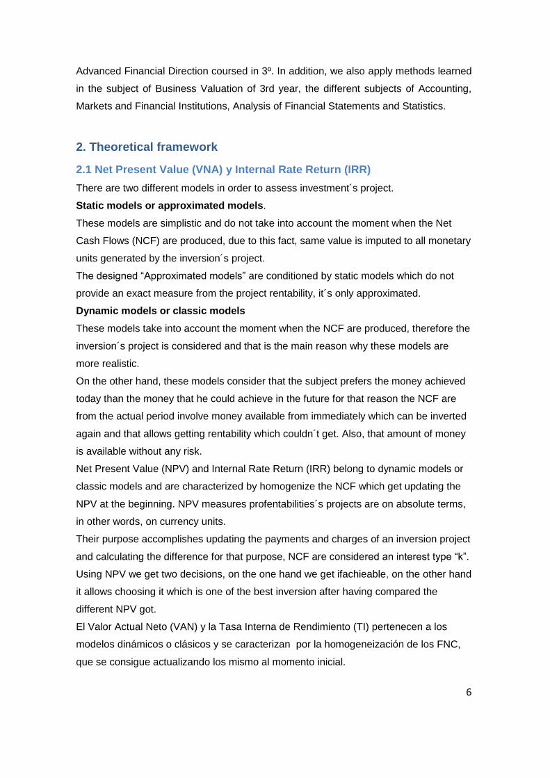
NPV formula is:
Where:
-A: initial investment Qj: Net Cash Flows k: financial cost j: number of periods The obtained result is analysed when NPV is applied:
If the NPV is positive (NPV 0): Inversion is accepted.
If the project is done the capital inverted could be recuperated as well.
● If the NPV is negative (NPV O): Inversion is not accepted
If the company makes the project, company´s wealth will decrease, with a net loss as
the amount got in the NPV.
If the NPV is equal to zero (NPV=0). Inversion is not accepted.
Realizar el proyecto resulta indiferente para la empresa ya que no va a generar ni
beneficios ni pérdidas.
Realising the project result indifferent for the company because it doesn´t make loss or
profit for the company. Financially it doesn´t make inversions in which the company is
not going to get earnings. (See Aragó, Balaguer, Cabedo, Matallín, Soler (2012)
Dirección financiera pp.67-70).
To sum up, the company has like objective maximise its market value, that is the
reason why when there are different inversion projects which are similar, distinguishing
and positive, it will be chosen one which offers the biggest NPV.
Some advantages of using the NPV to value projects are:
We can get useful predictions about the impact which the inversion project will have a
value´s company.
Also, NPV calculation considers cash flow expiration, in other words, NFC are
homogenised on time, minimizing to a unit measure amounts of money got in different
moments.
Some disadvantages that NTV include are the following: the difficulty to determinate
discount´s rate, positive NFC are immediately reinvested to an equal rate to discount
type, and negative NFC are financiered with resources whose financial cost is also at
the discount rate.
8
IRR is the rentability or interest rate which provides an inversion, It´s expressed on
percentage of one unit of increasing, which is the reason why IRR is a relative measure.
On the other hand, it is a brute measure because we have to discount financial cost
from the capital inverted on the project (k), that is the reason why when a project is
accepted o refused , IRR compares the brute relative rentability by monetary unit
inverted, “r”. The difference between both is a measure from the relative net rentability
by unit inverted on the project.
Rn = r - k
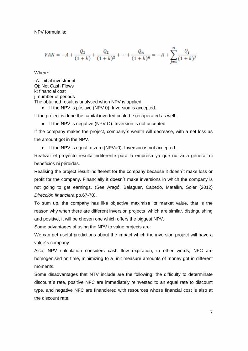
IRR formula is:
Where;
A: Initial investment
Qj: Net Cash Flows
j: Number of periods
The obtained result is analysed when IRR is applied:
If r> k : The project is accepted
The internal performance ´s rate got will be bigger than the minimal rentability
rate required to the inversion.
If r=k The project is not accepted
The inversion could be made in case of the competitive position from the company
improved and there wasn´t any alternative better.
If r< k: The project is not accepted
The minimal rentability required is not got.
The main advantage is that as the rentability is expressed on relative terms the unitary
money offers a better visualization than if it was on absolute terms. As well as, it values
at the same time all the amount of money which makes the project.
On the other hand, an important disadvantage is its calculation because the equation
sequence depends on the number of periods, that is the reason why it is said that the
result is inconsistent and few real.
9
There is an important relation between both approaches. Also, when they are used
correctly both provide the same outcome. Because the IRR is the rate discount which
would provide to the project a VNP of zero. That is the reason why we could use this
theory to calculate the rentability of a project with many cash flows, equalling the
formula to zero and keeping as question “r”.
When we compare IRR with the opportunity cost we know if the VNP is positive
because it will decrease when the discount rate increases. On the other hand, if both
parameters are compared, we have to considerate that both have limitations and
sometimes their results are inconsistent.
If we analyse how IRR and VNP study the rentability, we can see that VPN study the
rentability of unitary money while IRR makes a percentage. The same happens with
NCF, on the one hand, NPV takes into account the different expirations, giving priority
to the nearest on the time, reducing the risk and reinverting NFC to a discount rate “k”
used in the same analyse. On the other hand, IRR doesn´t study if NCF are reinverted
periodically on a rate “k”. It values a rentability “r”, valuating the capacity of inversion
from the project.
In relations with companies, when a project makes evaluation, it is usually used both
measurement bases, because how we have mentioned if they are used correctly, they
allow getting the same conclusion, but Brealey, Myers, Marcus, Mateus (2010)
Finanzas Corporativas pp.220-223 Say that IRR has some harmful defects, for
example:
Defect 1: lend or borrow?
The theory explains that VNP increases at the same time that discount rate decreases
in order to get a good result from the IRR. But if the company can lend that it will want
that IRR was high. On the other hand, if the company borrows that it will want that IRR
decreases. When VNP increases with interest rate, the IRR criterion is turned over. In
this case, the project would be accepted only if “r” is smaller than “k”.
Defect 2: Several rentability rate´s
In the case of cash flows, different sign changes can be made, in this case, the IRR
does not work correctly since more or fewer IRRs may arise as sign changes have or
even not find any IRRs, however the NPV gives a Good result always, without for him it
is an inconvenience the number of existing sign changes.
Defect 3: Projects mutually exclusive
If there are several projects, all rentable and exclusive, when we have to choose one of
them, we will choose that which offers the biggest VNP. On the other hand, when we
10
study IRR, it is not necessary to choose the biggest result because a big IRR is not a
PRINCIPIO, it is necessary to analyse different points to understand that fact.
Defect 4: Projects mutually exclusive with different disbursements.
When projects with the same duration and different initial disbursement are compared,
IRR can encourage mistakenly small projects with high rentability´s rate but with small
VAN.
2.2 Analyze of the Net Cash Flow and the problems on the application of its
calculation
Before estimate cash flow, it is important to consider normality on the behaviour of an
inversion project. The process has three stages.
Firstly, the start state, where is required inversions on floor, equipment and rolling fund
because products and feedstock are necessaries. The second stage is made at the
middle project, when cash flow derivate from sold operations are got, therefore in this
moment, we go on inverting on working capital.
The final phase would be given once the project has been liquidated, the equipment
and plants that had been acquired can be used for sale or other activities, if it were the
case of sale, the divestment of assets, entails inflow of Cash in addition to the sale of
products and the collection of outstanding bills. With this, it can be seen that the cash
flow of a project is the sum of the disinvestment of non-current assets, the net
investment in working capital and the cash flow of operations. .
The following are various aspects to identify Net Cash Flows and different problems
that arise when calculating:
Cash Flow
As mentioned in the previous section, to find the profitability of a project, the current
value is calculated by discounting the cash flows and not the result reflected in the
Annual Accounts. This is because according to the accounting principle of accrual, the
income and expenses are reflected in the real flow of goods and services and not when
the monetary flow derived from them. In addition, you must take into account that the
projects are financially attractive for the treasury they generate; therefore, the capital
budget should be based on the cash flow and not on the results of the Annual Accounts
Costs
There are different costs to consider making a correct valuation of the NCF, these are:
incremental cash flows, unrecoverable costs, opportunity cost and overheads.
It begins by analyzing how to obtain the incremental flows; Is the difference between
the cash flows derived from the investment and the cash flows that would have
11
occurred if the project had not been carried out. Similar to this situation is the
opportunity costs, which refer to the amount of capital, labor and materials used in one
project failing to make another.
With regard to the unrecoverable costs, they are past disbursements that will not be
possible to recover and that will remain regardless of whether or not the project will be
accepted, and will not affect its NPV.
Finally, when talking about general expenses refer, for example, to rentals, heating or
electricity. The consumption of these expenditures may not be directly related to the
project, although due to the principle of incremental cash flows only the extra costs
imposed by the project will be included in the investment estimate.
Working capital
The working capital or working capital is the difference between the current assets
composed of, the treasury, stocks, debtors and accounts receivable and the current
liabilities consisting of debit accounts payable.
Often mistakes are made in regard to working capital when cash flows are predicted;
They are calculated but not taken into account that this can vary or simply, omit that it
can be recovered at the end of the project, due to the entry of cash generated after the
stocks are exhausted and charged to customers their Debts incurred.
● Discount of nominal cash flows at nominal cost of capital
The actual cash flows are discounted at the real discount rate and the nominal rates at
nominal, both leading to the same updated result. It must be taken into account that the
quantities cannot be combined or equated with the different discount rates, since this
can constitute a serious error, due to the fact that the type Real interest rate on deposits
depends on inflation, and if it were possible to mix discount rates, inflation would not be
taken into account in predicting future cash flows, leading to an excessive reduction in
the value of the Project.
Separate investment and financing decisions
Regardless of how the project has been financed, it must be considered that it is
financed with equity capital, considering all cash outflows as coming from shareholders
and entries as if they were for them. This is done in order to separate the investment
decision analysis from the financing decision.
Investments in capital and working capital
Investments in fixed assets or working capital are components of cash flow, with
respect to capital investment; negative cash flows involve cash outflows and initially
exist in a project due to investment in non-current assets. On the other hand, when the
12
company divests, i.e. sells those assets, it generates positive cash flows. Yes, we are
referring to the working capital, the additional investments that are made on this when
the project is undertaken, for example, if you have to acquire raw material, it means
cash outflows. In addition, the treasury decreases when customers do not pay their
debts contracted with the company for the provision of services or receipt of
merchandise or for the accumulation of stocks of raw material or finished products.
When the project is finished, finished products have been sold and customers are
charged outstanding debts. Investments in working capital are reduced as it becomes
cash.
In summary, when investments are made, working capital increases and there are
negative cash flows; however, when working capital is reduced, it means positive cash
flows.
There are 3 methods for calculating the cash flows that derive from the operations.
METHOD 1. Monetary units that enter less leaving monetary units.
Only items in the income statement that represent cash flows are considered. The
income obtained is subtracted from the cash outflows and taxes paid, not considering
the amortization.
Cash flow from operations = Income - Cash out – Taxes
METHOD 2. Adjusted accounting benefits
This method starts with post-tax accounting benefits, plus deductions made for non-
monetary expenses, such as depreciation. Non-monetary expenses reduce profit but do
not affect cash flow.
Cash flow from operations = Profit after tax + Amortization
METHOD 3. Tax savings
The amortization deduction indirectly affects cash flows. This implies a method for
calculating the cash flows of operations; the net profit is calculated first assuming that
the amortization is zero remaining as follows:
(Income - cash flow) X (1-Tax rate).
Once this is done, the tax savings generated by the amortization are added. Next, the
operating cash flow is calculated as follows:
Cash flow from operations = (Income - Cash flow) X (1- Tax rate) + (Amortization x Tax
rate)
Finally, it is important to emphasize that investment projects are not only carried out
with the objective of having benefits, but can also be done to improve operating cash
flow and reduce costs.
13
2.3 Cost of capital, models for its calculation and problem in its application
According to Mascarenas (2015), companies continually have to decide where to invest
the incomes they have, in order to achieve the highest return with minimum risk. To
determine the acquisition of an asset that offers greater profitability, a set of possibilities
with equal risk requires a benchmark, the required rate of return, which allows the
investor to decide to make the concrete investment.
Each asset that is intended to be acquired will have an expected rate of return
established, when it is lower than the required rate of return, the investment will not be
realized, however, when higher will be accepted, since, it will increase the wealth of the
Investor with that decision.
The rate of return required by the company is also called cost of capital. This rate
shows, on the one hand, the cost of the resources of the company or others that are
invested in the project and, on the other hand, the discount rate that updates the flow of
cash flows that the company undertakes to generate. Therefore, when the risk is high
will imply a high capital cost, i.e. a higher discount rate and as a consequence a low
valuation of the company's securities and vice versa otherwise.
It is important that projects choose an appropriate rate of return required, since it allows
evaluating the feasibility of these. If a fee is used May lead to inappropriate
assessments.
The main problem that arises when determining the cost of capital is that, regardless of
the theorem chosen to find it, the same criteria are used without differentiating the type
of sector in which the company is located and without taking into account the inequality
in receiving information from investors and managers.
Before proceeding, a distinction is made between two concepts that can lead to
confusion; these are the cost of capital and the opportunity cost. The cost of capital is
what is reimbursed to third parties for their financial funds, represented in Balance
would be the liability, i.e. the cost of debt and in equity the cost of capital of
shareholders. On the other hand, the opportunity cost is what is not perceived when
investing the resources in the project.
Continuing with the cost of capital, the implicit factors that determine it are shown
below:
1. Economic conditions
It determines the demand and supply of capital, as well as the expected level of
inflation. This economic variable is reflected in the risk-free interest rate since it consists
of the real interest rate paid by the State and the expected inflation rate.
14
When the demand for money varies and supply is held steady, investors increase their
required rate of return, the same is true if inflation is expected to increase. On the other
hand, if the money supply increases or the price level is expected to fall, a decrease in
the yield required for each investment project will occur.
2. Market condition
At this point the concept of risk premium is introduced; it is the difference between the
required performance of a risky project and that of a similar but risk-free project.
When the risk of the project is increased, the investor will demand a higher required
rate of return; otherwise, if the risk decreases, the higher the risk the higher the risk
premium and vice versa. Likewise, if the asset is difficult to sell because it is not liquid,
the liquidity premium is much higher, making it increase even more the minimum
required yield.
3. Financial and operational conditions of the company
The risk is divided into two types; Economic risk, depends on the investment decisions
of the company and refers to the change in the return on assets and financial risk,
which refers to the financing decision; Use of debt and preferred shares, refers to the
variation of the yield obtained by the shareholders.
4. Amount of funding
When the company's financing needs increase, the cost of the company's capital varies
due to a number of reasons:
- When issuing securities, the issuance costs, which in relative terms, will be
lower, the higher the volume of the issuance, although the larger the volume of
shares issued, the greater the decrease in its Price in the market, which will
have an increase in the cost of capital.
- When the company requests a high volume of funding compared to its own size,
investors will doubt the ability of the board to manage it efficiently which will increase its
required performance. It is convenient to bear in mind that for all determinants,
whenever the required return increases, the cost of capital also does so.With regard to
risk, it can be divided into two parts, systematic and non-systematic. The systematic
depends on the decisions of the company and can be eliminated through an efficient
diversification of the money to be invested, while the unsystematic cannot be reduced
beyond a certain value, since it depends on the market. This differentiation is important
because, in certain cases, the risk premium of an investment project incorporates the
systematic risk to which it is exposed and not its specific risk that has been
appropriately eliminated through good diversification.
15
It is expensive and complicated to estimate the cost of capital, so to get an approximate
value is based on basic assumptions that simplify the calculation, these are:
- The economic risk does not change; the cost of capital of the company will be
adequate for those projects that have an economic risk equal to the assets in
the company.
- The capital structure does not change; on average the structure remains
constant, even if for a time varies, the goal is that in the long run it will remain
unchanged.
- The dividend policy does not vary, assuming dividends increase indefinitely at a
constant annual rate.
These hypotheses are limiting, therefore the model should be evaluated regularly in
addition to talking about a range and not a specific value in determining the cost of
capital, and then some models are shown for their calculation.
2.3.1 Determination of discount rate
There are different methodologies to determine the rate of profitability, in this section we
will highlight three of them, especially the CAPM or asset valuation model, since
according to the economist Damoran (2013) is one more methods used by financial
analysts.
Capital Asset Pricing Model (CAPM)
The objective of the CAPM is to explain how a financial asset is governed by historical
market behavior and also allows it to project its discount rate. Seeks to measure and
compensate market risk; predicts the relationship between the return of the asset and
its implied risk.
In order to understand this model we must first differentiate between two types of risk,
systematic and non-systematic, the systematic is not controllable by the company and
cannot be reduced through diversification as it depends on the market. In contrast, non-
systematic risk corresponds to the risk of the company, and can be mitigated by the use
of diversification, dispersing the capital between different assets.
It is assumed that the rate of return required by an investor is equal to the rate of risk-
free return that can be achieved in the financial market, plus a premium for the
assumption of the risks that arise when placing its capital in a Whose flows are less
predictable. It also includes Beta, which states that the company is exposed to market
risk, measures the sensitivity of the organization's profitability to the latter. When beta
takes a value equal to one the asset varies in the same way as the stock market,
inverse happens when beta is greater than one.
16
In order to harmonize the model, the following assumptions apply to the base theory:
- Investors are risk averse.
- All investors have the same time horizon.
- There is no capital limit borrowed at the risk free rate.
- Investments can be divided into unlimited shares and measures.
- There are no taxes, no inflation, no transaction costs.
These assumptions are not real when estimating a project, therefore they are
inconvenient, for example: not all investors have the same level of profitability and
expected risk, it is not studied the fact that there are investors who prefer to obtain a
return Lower to higher risk or that not all investors have access to the same information.
In addition, the model assumes that the market portfolio is efficient and this does not
have to happen always, as provided by economist Damodaran (2013), the company
beta may not be valid, because there is no single beta for all The investors. This results
in sometimes the betas being calculated in relation to the historical dates, making
mistakes, since they are not normalized to Because of not using the same time horizon
in its calculation and at the same time use different yields, this has repercussions on the
stock index taken as reference to carry out the calculation. The economist adds that
using the beta calculated with historical dates is equivalent to valuing the company
without analyzing the actions or the future perspective of the company, for the valuation
of projects, this fact is very dangerous. Regarding the risk-free rate there are also some
discrepancies, since in general the companies follow the recommendations that
Mascareña (2015) sets out to define the rate of risk-free asset required in the equation
that will be explained later, Using the 10-year State Bond interest rate because the
duration of this issue is similar to that of the cash flows of the companies to be valued,
the durability of the asset without risk is similar to the Of the stock market index used to
calculate the market and beta performance, but it is not known with certainty if the state
debt is indeed risk free since in some countries throughout economic history have not
faced the Debts they had with their creditors. That is why Damodaran (2013) states that
it does not really know what the risk-free rate would be.
With all of this, it is concluded that, despite its empirical importance, the CAPM model is
fixed on parameters that question its validity. For them, it must be verified if the CAPM
model is valid for the project to be analyzed.
Weighted Average Cost of Capital model (WACC)
This model estimates the sum of all sources of capital; The cost of indebtedness and
the cost of investment of the shareholders of the company, weighted by their share in
17
the capital structure, with this, can determine how much interest a company has for
each monetary unit it finances. When the company's WACC increases as the beta
increases and the rate of return on capital increases, it means a decrease in valuation
and an increase in risk.
The calculation of the WACC is divided into three parts, on the one hand the cost of
capital, the amount that a company must spend to maintain a share price that satisfies
its investors. On the other hand, the cost of debt, to determine it, uses the market rate
that the company is currently paying on its debt. The last part to consider would be the
taxes, since for those companies with debt, supposes a subsidy of the State.
The WACC is the minimum acceptable rate of return at which a company offers returns
to its investors. To determine the personal returns of an investor on an investment, the
WACC is subtracted from the percentage of performance of the company. On the other
hand, if the return of the company is less than WACC, the company is losing value,
meaning potential investors would be better off putting their money somewhere else.
The limitations to be considered on this model are: the difficulty in its calculation and
although its use can help give a useful view of the company, it will always have to be
used together with other metrics when deciding whether to invest or not .
After studying various methods, the one chosen to estimate the discount rate will be the
CAPM, since according to someone is the one that comes closest to reality
Coste Medio Ponderado de Capital más una prima de riesgo.
This model presents significant difficulties in determining its performance for three
reasons; In the first place, the market rate no longer includes a risk factor; second,
subjective correction factors afflict the projects, because they arbitrarily add an
opportunity cost and third, the determination of the risk premium is subjective since It is
currently difficult to determine due to the existing turbulent environment, as would occur
if historical data were used because of volatility in the market.
18
3. Viability study
To begin this point, an overview of the organization is presented, as well as an
explanation of what the investment project will consist of. In the Annexes section,
Annex 1 and 2 show the Balance Sheet and the Profit and Loss Account Respectively,
for the 2014 and 2015 periods.
The company in which the investment project is to be developed is an SME whose
corporate purpose is the manufacture of ceramic material of all kinds, especially tiles
and pavements, as well as their distribution and commercialization, as well as
complementary complementary activities for such purposes. Since 2013 the evolution
of this company has been favorable, yielding over time positive results in 2013 of
36,742 euros in 2014 27 thousand euros and in 2015 of 399 thousand euros the jump
from one benefit to another has been considerable, Which is why at first glance there
should be no drawbacks in the investment since it shows a steady evolution.
Negative issues to highlight about the company are the energy consumption costs,
since the evolution of the price of these costs, which are required for the operation of
the company, specifically to carry out the production process, in recent years has gone
increasing. For this reason they must continually look for different actions to reduce any
type of cost existing in the company, this is the reason that has triggered to make the
following investment project. This is to acquire two automatic dozers that would form
part of the existing machinery in the final process of the production of the product, since
currently the work of depositing in boxes the tiles were done manually by the
employees. In addition, the embedding machines incorporate a technology that has as
a purpose to consume less electrical energy, with all the mentioned aspects it is
intended that the incorporation of the two automatic dozers will reduce costs.
According to the opinion of the financial director of the organization to study the
investment project, we would be facing a company of sustained growth that in the long
term, thanks to the quality of the product will enable them to consolidate their position in
the market and maintain the path of profits.
At this point we will first proceed to the determination of the discount rate, in section 3.1
and then in section 3.2 we will calculate the Net Cash Flows obtained, these in point 3.3
can be observed by calculating The NPV and the IRR if the project is viable. If the
previous results were positive and the IRR was greater than the discount rate
calculated in accordance with the main objective of determining whether the project will
be viable, different feasibility analysis procedures will be carried out, including The
scenario analysis carried out in point 3.4 and the sensitivity analysis carried out in 3.5.
19
In order to do so, the company has provided data in addition to the annual accounts for
2014 and 2015.
3.1 Discount rate determination In the following section, the discount rate is to be determined, using the CAPM, the
asset valuation model, since, as mentioned in its explanation, it is one of the most used
methods by financial analysts, Its simplicity and logic on which it is based, as well as
being one of the closest to reality. With the CAPM you get the performance of the
company that is correlated with the market. The general equation of the model is:
E [Ri] = Rf +E [βM - Rf] βi
Where:
E [Ri] = Expected return on investment.
Rf = Risk-free return on assets
ΒM = Expected market return over the considered period of time
[ΒM- Rf] = Value of the risk premium
ßi = Volatility coefficient
It can be seen that the uncertainty of the equation is the expected profitability of the
investment project and that the formula is composed of: a risk-free asset, the expected
risk premium of the market and the beta of the market. Next we proceed to explain how
the data were obtained, taking into account the different dilemmas that have been
exposed previously.
First, to find the value of the risk-free asset, the recommendations of Mascarenas
(2015) mentioned in the definition have been followed. Therefore, the profitability of a
Spanish State Bond with a 10-year maturity has been taken into account, this has been
found through the Public Treasury website on May 25, 2017, the average interest rate
of said asset Risk free was 0.590%.
Second, in order to determine the expected risk premium we pay attention to its
constitution, it is equal to the expected average market return minus the risk-free return
of the asset. In the previous point we solved a part, to determine the second
component, the average expected market yield, which according to authors Brealey,
Myers, Marcus and Mateos-Aparici (2010) the market portfolio must contain all the
assets of the world economy And not only shares but also bonds, foreign securities or
real estate assets. But in practice, financial analysts use financial market indices and
usually the Standard & Pool Composite Index (the S & P 500). Reason for which this
20
index was chosen, which on May 25, 2017 yielded a dividend yield of 8.23%. Therefore,
the value of the expected risk premium will be 7.64%.
Third, to get the beta of the equation, it is convenient to know what kind of company we
are in, this is a company that, like so many in Castellón, is dedicated to ceramics. It is
true that, in times not too distant, shortly before the crisis broke out, ceramic companies
had as clients large companies dedicated to construction and that during this period
these companies became strong in addition to provoking a growth not only of the
companies themselves Existing ones but those that were new to the sector, since there
was so much presence of this type of companies in the market, to differentiate and
acclaim more customers had to differentiate by launching new products or modifying
existing ones. Which to this day also do? After the crisis, construction has declined in
Spain and many of the ceramic companies had to close, remaining in the market those
who have decided to export to other territories where construction is booming,
especially countries like Saudi Arabia, United Arab Emirates, Qatar, Dubai and Bahrain.
It can be observed that we are facing a sector that depends a lot on the economy,
mainly for the construction and followed by if in general the population does not own
any wealth nor will they make reforms that require tiles in their houses or companies.
Consequently, and referring to the company in which the Investment project has a small
size and its client portfolio is present in 55 countries, therefore, we are facing an
organization that has been open to the market. Of the market at all times. The design of
its products is aimed at companies as well as individuals.
As it has not been possible to obtain historical data of companies of the ceramics that
are listed on the stock market, the market and the position of the company in it have
been studied. Based on the study in the sector of Basic materials, industry and
construction, because according to the institution stock exchanges and markets, the
denomination of this sector encompasses the companies engaged in some economic
activity related to the extraction and / or treatment of minerals, Metals and their
transformation, manufacture and assembly of equipment goods and general
construction activities and construction materials.
For all that, the beta that has been found after reading different articles of analysts,
approaching as much as possible to the reality, since finding a beta of a sector is
general and complicated to adjust to the company, therefore must have Considering
that this value is subjective because it is not listed on the stock market and that a
change in it would imply a change in the CAPM result. The value of beta is 1.31
because it is a sector that depends on other sectors, although not all of its products go
21
solely and exclusively to construction companies if it is true that most of them is
directed to new constructions.
Obtaining the different factors that are included in the CAPM equation, we can already
calculate the value of the expected return on investment:
[𝑅𝑖]=0, 59%+ [7, 64%] ×1, 31=0, 1060=10, 60%
Determining the expected return on investment, we obtain that the discount rate to be
used for the study, this is 10.60%.
3.2 Calculation Net Cash Flows
In the following section, Net Cash Flows will be calculated, only the charges and
payments or expenses and revenues caused or belonging to the investment to be made
will be taken into account. Increases or decreases of each of the items will be used in
order to differentiate the ones that the company has, from those that would have in the
case of making the investment. The objective of calculating Net Cash Flows is to know
if the company should carry out the project or to evaluate other aspects that lead to
profitability.
As mentioned in the introduction of the point being developed, the investment to be
made is the acquisition of two automatic cash dispensers, which would result in an
increase in fixed assets of € 217,935, which would be located in the final process of the
production chain, Work, is done by the staff of the company. The time horizon that is
proposed to make the study of the feasibility of the project is 10 years, because it is the
useful life of automatic dozers. The patrimonial masses that will be altered with the
investment project are explained below; the results of the same ones are obtained
realizing a future projection of the predictions.
SALES
The fact of incorporating the automatic dozers is related to an increase of sales, since,
at the moment they cannot satisfy all the demand because the packaging do it of
manual way, causing that the requested orders cannot be reached. For this reason,
with the incorporation of automatic dozers, an increase in sales is anticipated by the
inclusion of new customers that can be admitted. It should be taken into account that
each customer has a different billing, and not knowing how much corresponds to each
one, has divided the number of customers into three classes, according to the quality;
High, medium and low. The company has provided me with information to be able to
classify in the three blocks the 1,500 clients that it currently has. In addition, we also
obtained the amount of the sales figure corresponding to the years 2013, 2014 and
2015 that has been divided by the volume invoiced by each type of customer. Assuming
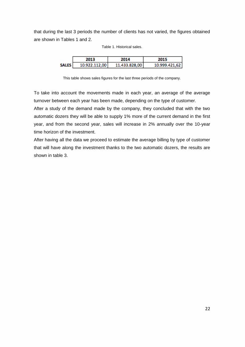
22
that during the last 3 periods the number of clients has not varied, the figures obtained
are shown in Tables 1 and 2.
Table 1. Historical sales.
This table shows sales figures for the last three periods of the company.
To take into account the movements made in each year, an average of the average
turnover between each year has been made, depending on the type of customer.
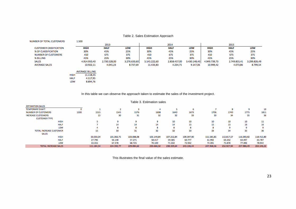
After a study of the demand made by the company, they concluded that with the two
automatic dozers they will be able to supply 1% more of the current demand in the first
year, and from the second year, sales will increase in 2% annually over the 10-year
time horizon of the investment.
After having all the data we proceed to estimate the average billing by type of customer
that will have along the investment thanks to the two automatic dozers, the results are
shown in table 3.
23
Table 2. Sales Estimation Approach
In this table we can observe the approach taken to estimate the sales of the investment project.
Table 3. Estimation sales
This illustrates the final value of the sales estimate.

24
AMORTIZATION
The purchase of the two automatic dozers is an endowment of the annual amortization.
The calculations will be made in a common way, without differentiating by fitters. The
amortization percentage is obtained from the amortization tables of the Corporate
Income Tax Law, using the straight-line method of amortization defined in article 12.1 of
the Corporate Tax Law and article 4 of the Corporate Income Tax Regulations. In
general, in order to make it easier for companies to determine the deductions for
corporate tax, they determine the depreciation according to the tables set forth in the
Corporate Income Tax Law, which is why the amortization calculation has been used
This method as I believe it is closer to reality. According to this law you can choose both
a period and amortization coefficient that lies between the limits defined below:
Linear coefficient maximum: 12%, is in the table
Minimum linear coefficient: 100 / maximum amortization period = 100/18 = 6%
Period of maximum years: 18 years, is in the table
Minimum period of years: 100 / Maximum amortization coefficient = 100/12 = 8.33 years
According to the data provided by the company, the packers have a useful life of 10,
this period is between the values determined in the previous paragraph, and the
resulting coefficient is 10%. After the following calculations, table 4 Increase of
amortization that will be effected for each year or what is the same the amortization
corresponding to the automatic dozers:
Table 4. Fit machines amortization
En la tabla se muestra la amortización total correspondiente a las encajadoras.
PERSONAL EXPENSES
Although the number of employees in this section will decrease with the automatic
dozers, they will be relocated to other sections of the production process. In addition, as
mentioned in the sales section, an increase is expected Of these due to the
incorporation of the new fixed assets due to the fact of supplying a greater demand,
therefore this will have an impact on an increase of the employees. The amount is
estimated in a total of 5 more employees in the company, throughout the investment.
These will be distributed as follows:El primer año:
- 1 technical engineer in charge of the section of packaging and 1 commercial
whose function will be to establish relations with new clients.
- The second year will include 2 more workers in plant.
25
- The third year, will require 1 administrative due to the workload that is
anticipated in these exercises.
According to convenio colectivo de 2017 para la Industria de Azulejos, Pavimentos y
Baldosas Cerámicas de la Comunidad Valenciana The balances to be received
depending on the job position is:
● Professional group. 2. Controls and technical first level.
Technician and head of production in plants of great dimension, technical director in
plants of small dimension, head of maintenance, responsible of design.
● Professional group 3. Coordinators and technicians. Commercial
● Professional group 5. Second level professionals
Operators of grinding, spray drying, pressing or extrusion processes, polish preparation
and application, polishing.
Horneros, classifiers, drivers of forklifts, electromechanical tasks of elementary level or
laboratory auxiliary.
● Professional group 6. Professionals. General criteria. They will include:
manual operations or simple machines that do not require training
● Professional group 4. Professionals first level. Manual operations or
simple machines that do not require training. Administrative
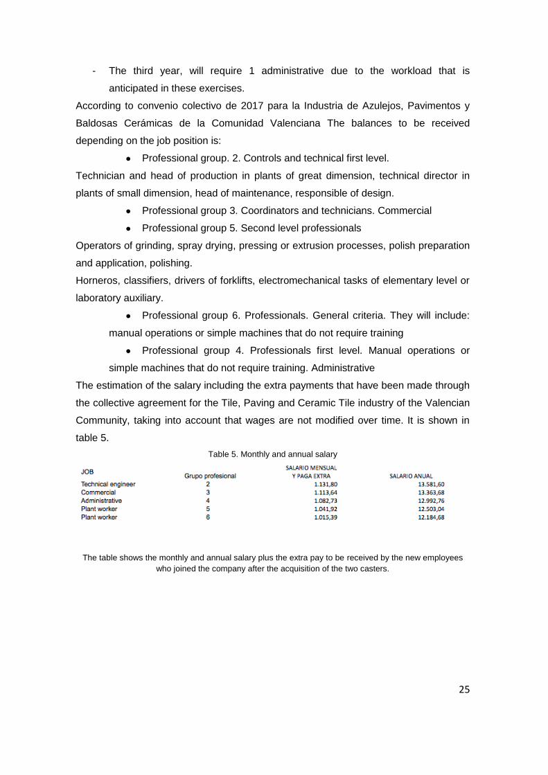
The estimation of the salary including the extra payments that have been made through
the collective agreement for the Tile, Paving and Ceramic Tile industry of the Valencian
Community, taking into account that wages are not modified over time. It is shown in
table 5.
Table 5. Monthly and annual salary
The table shows the monthly and annual salary plus the extra pay to be received by the new employees
who joined the company after the acquisition of the two casters.
26
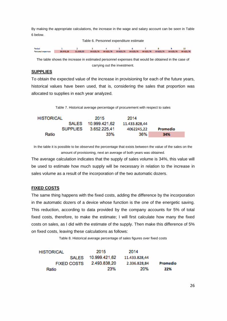
By making the appropriate calculations, the increase in the wage and salary account can be seen in Table
6 below.
Table 6. Personnel expenditure estimate
The table shows the increase in estimated personnel expenses that would be obtained in the case of
carrying out the investment.
SUPPLIES
To obtain the expected value of the increase in provisioning for each of the future years,
historical values have been used, that is, considering the sales that proportion was
allocated to supplies in each year analyzed.
Table 7. Historical average percentage of procurement with respect to sales
In the table it is possible to be observed the percentage that exists between the value of the sales on the
amount of provisioning, next an average of both years was obtained.
The average calculation indicates that the supply of sales volume is 34%, this value will
be used to estimate how much supply will be necessary in relation to the increase in
sales volume as a result of the incorporation of the two automatic dozers.
FIXED COSTS
The same thing happens with the fixed costs, adding the difference by the incorporation
in the automatic dozers of a device whose function is the one of the energetic saving.
This reduction, according to data provided by the company accounts for 5% of total
fixed costs, therefore, to make the estimate; I will first calculate how many the fixed
costs on sales, as I did with the estimate of the supply. Then make this difference of 5%
on fixed costs, leaving these calculations as follows:
Table 8. Historical average percentage of sales figures over fixed costs
27
In the table you can see the percentage that exists between the value of sales over fixed costs, then an
average of the result between both years was obtained.
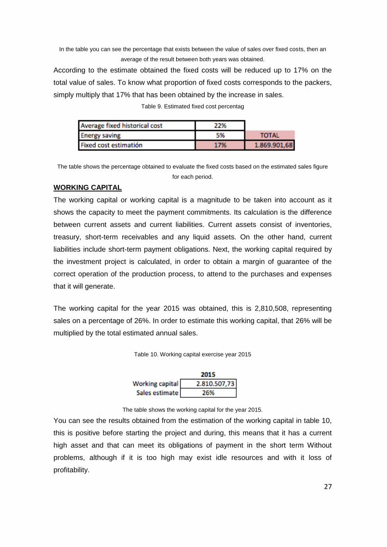
According to the estimate obtained the fixed costs will be reduced up to 17% on the
total value of sales. To know what proportion of fixed costs corresponds to the packers,
simply multiply that 17% that has been obtained by the increase in sales.
Table 9. Estimated fixed cost percentag
The table shows the percentage obtained to evaluate the fixed costs based on the estimated sales figure
for each period.
WORKING CAPITAL
The working capital or working capital is a magnitude to be taken into account as it
shows the capacity to meet the payment commitments. Its calculation is the difference
between current assets and current liabilities. Current assets consist of inventories,
treasury, short-term receivables and any liquid assets. On the other hand, current
liabilities include short-term payment obligations. Next, the working capital required by
the investment project is calculated, in order to obtain a margin of guarantee of the
correct operation of the production process, to attend to the purchases and expenses
that it will generate.
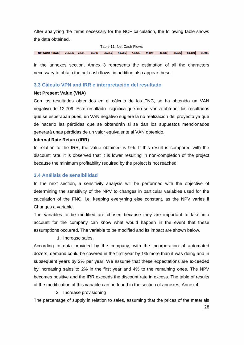
The working capital for the year 2015 was obtained, this is 2,810,508, representing
sales on a percentage of 26%. In order to estimate this working capital, that 26% will be
multiplied by the total estimated annual sales.
Table 10. Working capital exercise year 2015
The table shows the working capital for the year 2015.
You can see the results obtained from the estimation of the working capital in table 10,
this is positive before starting the project and during, this means that it has a current
high asset and that can meet its obligations of payment in the short term Without
problems, although if it is too high may exist idle resources and with it loss of
profitability.
28
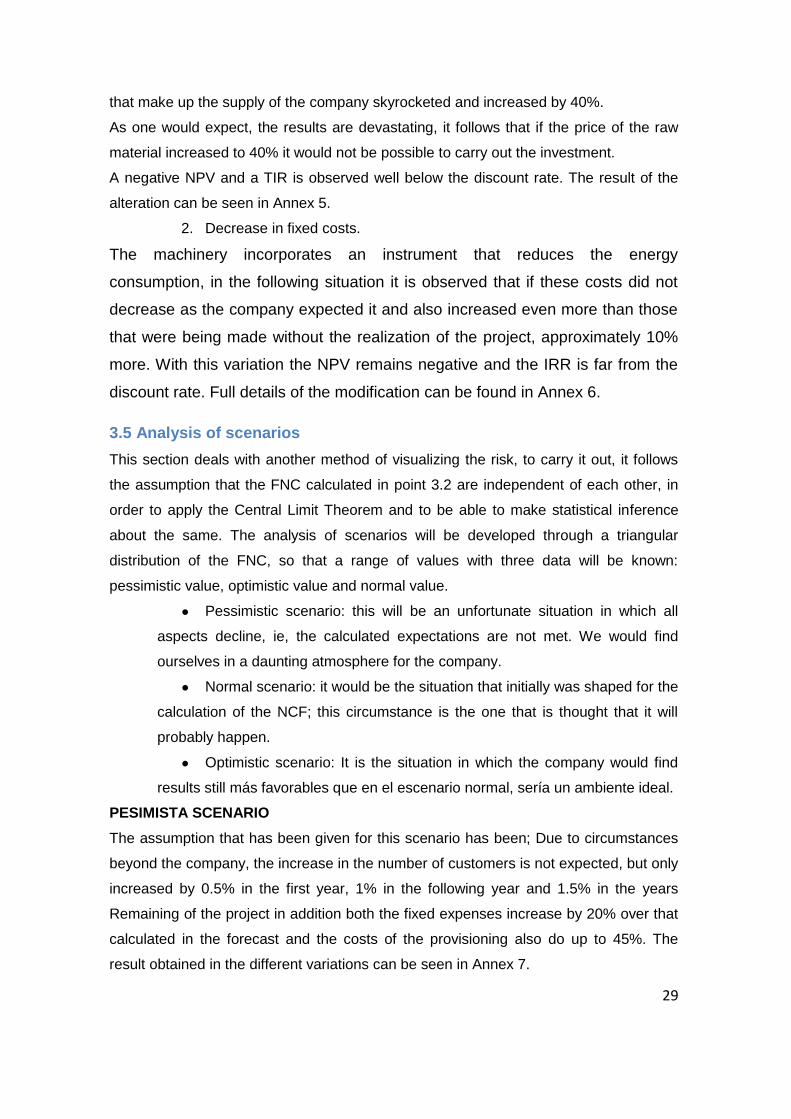
After analyzing the items necessary for the NCF calculation, the following table shows
the data obtained.
Table 11. Net Cash Flows
In the annexes section, Annex 3 represents the estimation of all the characters
necessary to obtain the net cash flows, in addition also appear these.
3.3 Cálculo VPN and IRR e interpretación del resultado
Net Present Value (VNA)
Con los resultados obtenidos en el cálculo de los FNC, se ha obtenido un VAN
negativo de 12.709. Éste resultado significa que no se van a obtener los resultados
que se esperaban pues, un VAN negativo sugiere la no realización del proyecto ya que
de hacerlo las pérdidas que se obtendrán si se dan los supuestos mencionados
generará unas pérdidas de un valor equivalente al VAN obtenido.
Internal Rate Return (IRR)
In relation to the IRR, the value obtained is 9%. If this result is compared with the
discount rate, it is observed that it is lower resulting in non-completion of the project
because the minimum profitability required by the project is not reached.
3.4 Análisis de sensibilidad
In the next section, a sensitivity analysis will be performed with the objective of
determining the sensitivity of the NPV to changes in particular variables used for the
calculation of the FNC, i.e. keeping everything else constant, as the NPV varies if
Changes a variable.
The variables to be modified are chosen because they are important to take into
account for the company can know what would happen in the event that these
assumptions occurred. The variable to be modified and its impact are shown below.
1. Increase sales.
According to data provided by the company, with the incorporation of automated
dozers, demand could be covered in the first year by 1% more than it was doing and in
subsequent years by 2% per year. We assume that these expectations are exceeded
by increasing sales to 2% in the first year and 4% to the remaining ones. The NPV
becomes positive and the IRR exceeds the discount rate in excess. The table of results
of the modification of this variable can be found in the section of annexes, Annex 4.
2. Increase provisioning
The percentage of supply in relation to sales, assuming that the prices of the materials
29
that make up the supply of the company skyrocketed and increased by 40%.
As one would expect, the results are devastating, it follows that if the price of the raw
material increased to 40% it would not be possible to carry out the investment.
A negative NPV and a TIR is observed well below the discount rate. The result of the
alteration can be seen in Annex 5.
2. Decrease in fixed costs.
The machinery incorporates an instrument that reduces the energy
consumption, in the following situation it is observed that if these costs did not
decrease as the company expected it and also increased even more than those
that were being made without the realization of the project, approximately 10%
more. With this variation the NPV remains negative and the IRR is far from the
discount rate. Full details of the modification can be found in Annex 6.
3.5 Analysis of scenarios
This section deals with another method of visualizing the risk, to carry it out, it follows
the assumption that the FNC calculated in point 3.2 are independent of each other, in
order to apply the Central Limit Theorem and to be able to make statistical inference
about the same. The analysis of scenarios will be developed through a triangular
distribution of the FNC, so that a range of values with three data will be known:
pessimistic value, optimistic value and normal value.
● Pessimistic scenario: this will be an unfortunate situation in which all
aspects decline, ie, the calculated expectations are not met. We would find
ourselves in a daunting atmosphere for the company.
● Normal scenario: it would be the situation that initially was shaped for the
calculation of the NCF; this circumstance is the one that is thought that it will
probably happen.
● Optimistic scenario: It is the situation in which the company would find
results still más favorables que en el escenario normal, sería un ambiente ideal.
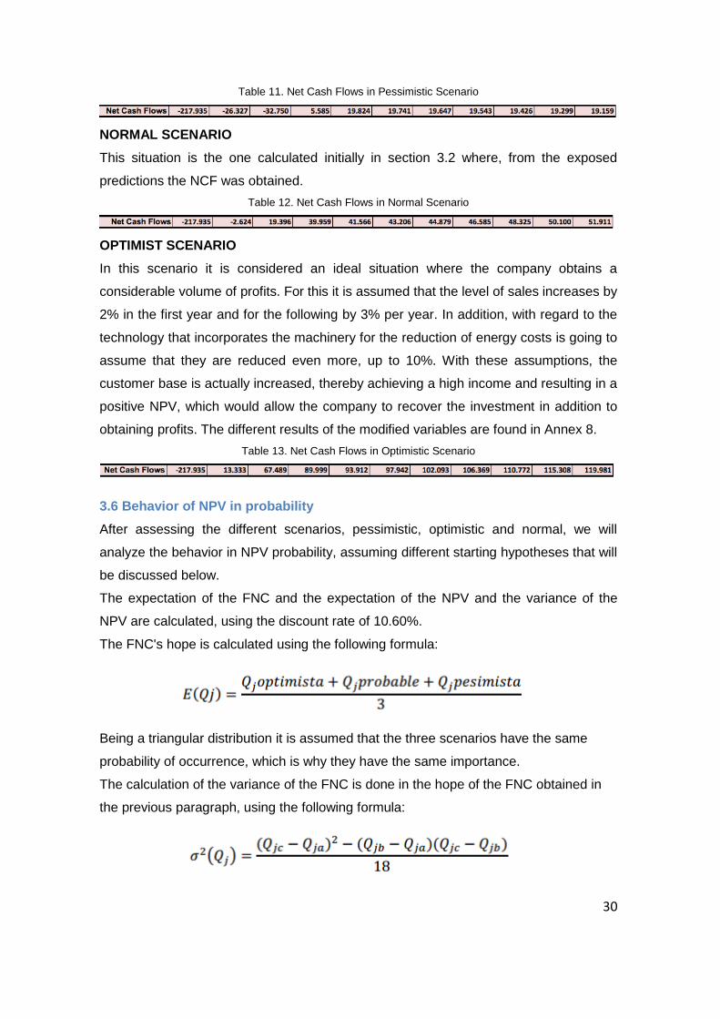
PESIMISTA SCENARIO
The assumption that has been given for this scenario has been; Due to circumstances
beyond the company, the increase in the number of customers is not expected, but only
increased by 0.5% in the first year, 1% in the following year and 1.5% in the years
Remaining of the project in addition both the fixed expenses increase by 20% over that
calculated in the forecast and the costs of the provisioning also do up to 45%. The
result obtained in the different variations can be seen in Annex 7.
30
Table 11. Net Cash Flows in Pessimistic Scenario
NORMAL SCENARIO
This situation is the one calculated initially in section 3.2 where, from the exposed
predictions the NCF was obtained.
Table 12. Net Cash Flows in Normal Scenario
OPTIMIST SCENARIO
In this scenario it is considered an ideal situation where the company obtains a
considerable volume of profits. For this it is assumed that the level of sales increases by
2% in the first year and for the following by 3% per year. In addition, with regard to the
technology that incorporates the machinery for the reduction of energy costs is going to
assume that they are reduced even more, up to 10%. With these assumptions, the
customer base is actually increased, thereby achieving a high income and resulting in a
positive NPV, which would allow the company to recover the investment in addition to
obtaining profits. The different results of the modified variables are found in Annex 8.
Table 13. Net Cash Flows in Optimistic Scenario
3.6 Behavior of NPV in probability
After assessing the different scenarios, pessimistic, optimistic and normal, we will
analyze the behavior in NPV probability, assuming different starting hypotheses that will
be discussed below.
The expectation of the FNC and the expectation of the NPV and the variance of the
NPV are calculated, using the discount rate of 10.60%.
The FNC's hope is calculated using the following formula:
Being a triangular distribution it is assumed that the three scenarios have the same
probability of occurrence, which is why they have the same importance.
The calculation of the variance of the FNC is done in the hope of the FNC obtained in
the previous paragraph, using the following formula:
31
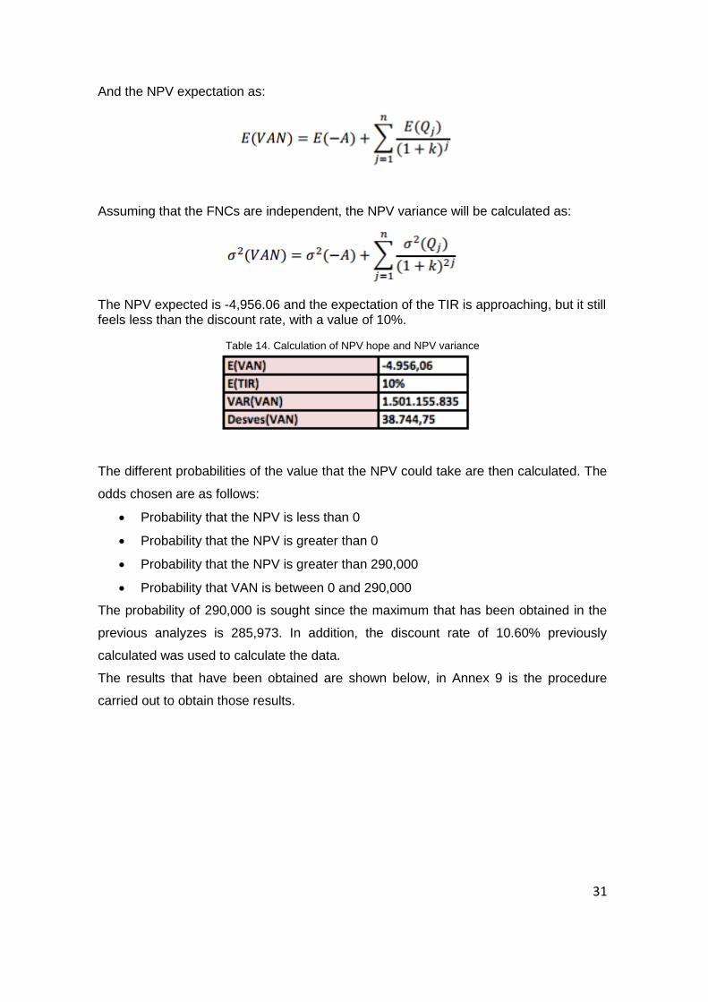
And the NPV expectation as:
Assuming that the FNCs are independent, the NPV variance will be calculated as:
The NPV expected is -4,956.06 and the expectation of the TIR is approaching, but it still feels less than the discount rate, with a value of 10%.
Table 14. Calculation of NPV hope and NPV variance
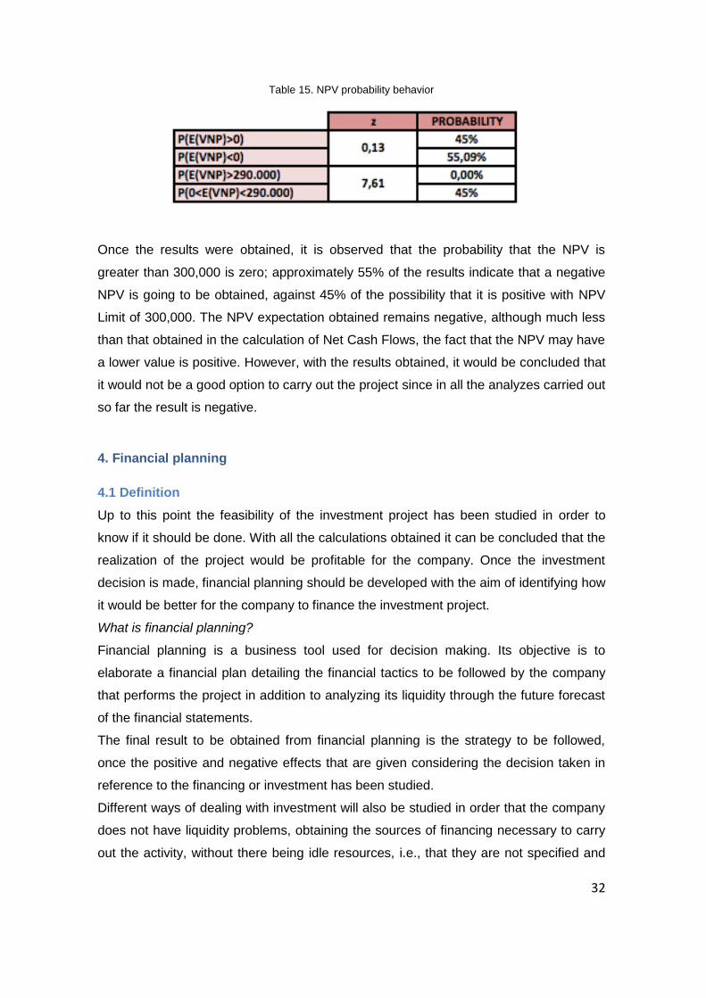
The different probabilities of the value that the NPV could take are then calculated. The
odds chosen are as follows:
Probability that the NPV is less than 0
Probability that the NPV is greater than 0
Probability that the NPV is greater than 290,000
Probability that VAN is between 0 and 290,000
The probability of 290,000 is sought since the maximum that has been obtained in the
previous analyzes is 285,973. In addition, the discount rate of 10.60% previously
calculated was used to calculate the data.
The results that have been obtained are shown below, in Annex 9 is the procedure
carried out to obtain those results.
32
Table 15. NPV probability behavior
Once the results were obtained, it is observed that the probability that the NPV is
greater than 300,000 is zero; approximately 55% of the results indicate that a negative
NPV is going to be obtained, against 45% of the possibility that it is positive with NPV
Limit of 300,000. The NPV expectation obtained remains negative, although much less
than that obtained in the calculation of Net Cash Flows, the fact that the NPV may have
a lower value is positive. However, with the results obtained, it would be concluded that
it would not be a good option to carry out the project since in all the analyzes carried out
so far the result is negative.
4. Financial planning
4.1 Definition
Up to this point the feasibility of the investment project has been studied in order to
know if it should be done. With all the calculations obtained it can be concluded that the
realization of the project would be profitable for the company. Once the investment
decision is made, financial planning should be developed with the aim of identifying how
it would be better for the company to finance the investment project.
What is financial planning?
Financial planning is a business tool used for decision making. Its objective is to
elaborate a financial plan detailing the financial tactics to be followed by the company
that performs the project in addition to analyzing its liquidity through the future forecast
of the financial statements.
The final result to be obtained from financial planning is the strategy to be followed,
once the positive and negative effects that are given considering the decision taken in
reference to the financing or investment has been studied.
Different ways of dealing with investment will also be studied in order that the company
does not have liquidity problems, obtaining the sources of financing necessary to carry
out the activity, without there being idle resources, i.e., that they are not specified and
33
are Have already claimed that it would lead to a decline in profitability.
In summary, the task to be performed at this point is the search for sources of financing
that is optimal and sufficient so that there are no liquidity problems. To achieve these
following requirements must be followed:
- It must be foreseen as probable and improbable, beneficial or harmful to the
company
- Training Optimal Financing
- Determine if the path followed is feasible and if not modify it so that it is.Se van
a formular diferentes estrategias basadas en supuestos futuros, determinado
para ello la planificación mediante procesos de prueba y error.
In addition, the capital budget will be discussed to assess, identify and develop
profitable investment opportunities for the company, checking whether the cash flows
generated by the investment exceed the funding flows required to execute the project.
What would happen if a capital budget were wrongly developed?
The consequences would be extremely serious, since it can mean a success or failure
for a company, for example, in those industrial enterprises that require a large
disbursement in assets, if the decision on what type of Immobilized invest, would lead
to great losses and can be translated into bankruptcy of the company.
4.2. Determination of the profit and loss account and the capital budget
The company's income statement and capital budget are then analyzed for a three-year
period, whereby different financing channels and the effect they will have on the
company will be studied.
It is important that the feasibility of the project be cost-effective to develop this section.
Given that the results obtained were in all the analyzes have been negative except for
the optimistic scenario, it will be the one used for the development of this point, since if
such circumstances occurred the project could be viable. The net cash flows that were
obtained can be seen in Annex 11.
To determine the provisional profit and loss account and the capital budget I have
based myself on 4 proposals:
Without external financing.
Capital increase
Long-term French loan.
Capital increase + Long-term French loan.
Due to the situation in which the company is, sustained growth, it does not distribute
34
dividends since the benefits obtained are reinvested in society.
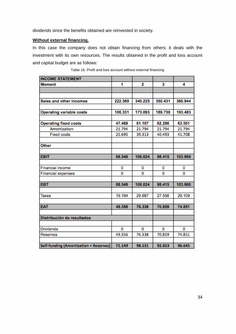
Without external financing.
In this case the company does not obtain financing from others; it deals with the
investment with its own resources. The results obtained in the profit and loss account
and capital budget are as follows:
Table 16. Profit and loss account without external financing
35
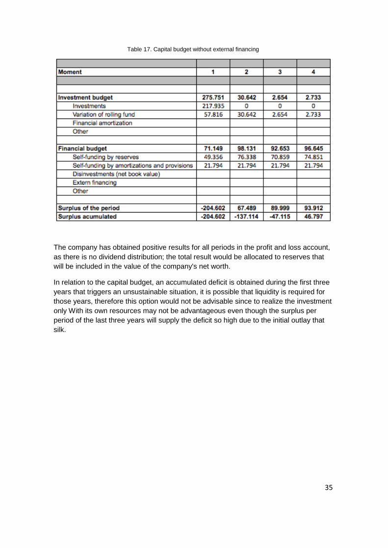
Table 17. Capital budget without external financing
The company has obtained positive results for all periods in the profit and loss account,
as there is no dividend distribution; the total result would be allocated to reserves that
will be included in the value of the company's net worth.
In relation to the capital budget, an accumulated deficit is obtained during the first three
years that triggers an unsustainable situation, it is possible that liquidity is required for
those years, therefore this option would not be advisable since to realize the investment
only With its own resources may not be advantageous even though the surplus per
period of the last three years will supply the deficit so high due to the initial outlay that
silk.
36
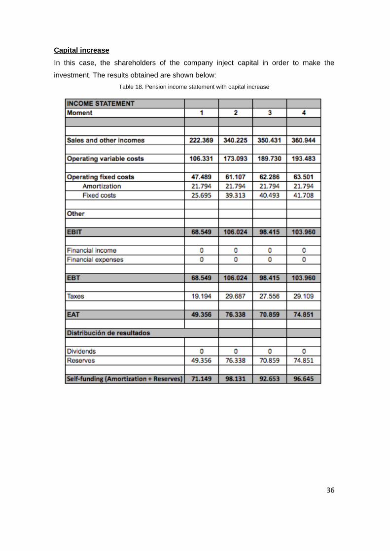
Capital increase
In this case, the shareholders of the company inject capital in order to make the
investment. The results obtained are shown below:
Table 18. Pension income statement with capital increase
37
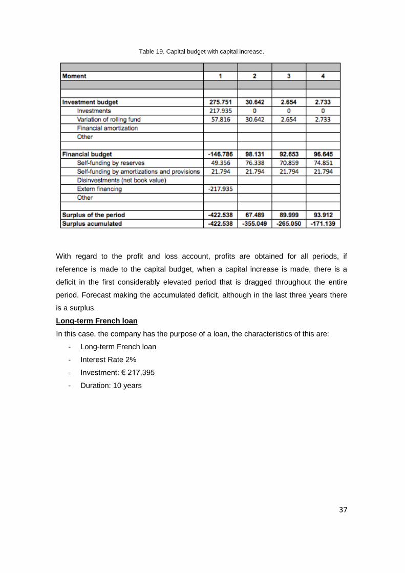
Table 19. Capital budget with capital increase.
With regard to the profit and loss account, profits are obtained for all periods, if
reference is made to the capital budget, when a capital increase is made, there is a
deficit in the first considerably elevated period that is dragged throughout the entire
period. Forecast making the accumulated deficit, although in the last three years there
is a surplus.
Long-term French loan
In this case, the company has the purpose of a loan, the characteristics of this are:
- Long-term French loan
- Interest Rate 2%
- Investment: € 217,395
- Duration: 10 years

38
Table 20. French Loan Repayment
39
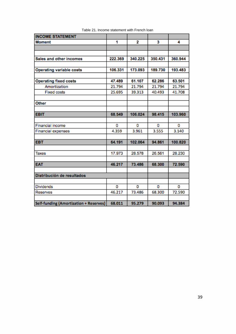
Table 21. Income statement with French loan
40
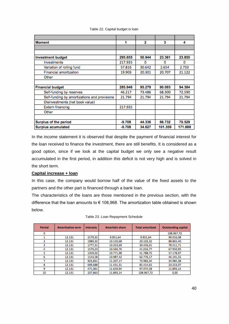
Table 22. Capital budget is loan
In the income statement it is observed that despite the payment of financial interest for
the loan received to finance the investment, there are still benefits. It is considered as a
good option, since if we look at the capital budget we only see a negative result
accumulated in the first period, in addition this deficit is not very high and is solved in
the short term.
Capital increase + loan
In this case, the company would borrow half of the value of the fixed assets to the
partners and the other part is financed through a bank loan.
The characteristics of the loans are those mentioned in the previous section, with the
difference that the loan amounts to € 108,968. The amortization table obtained is shown
below.
Table 23. Loan Repayment Schedule
41
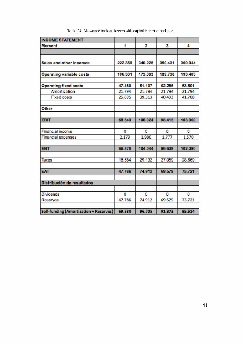
Table 24. Allowance for loan losses with capital increase and loan
42
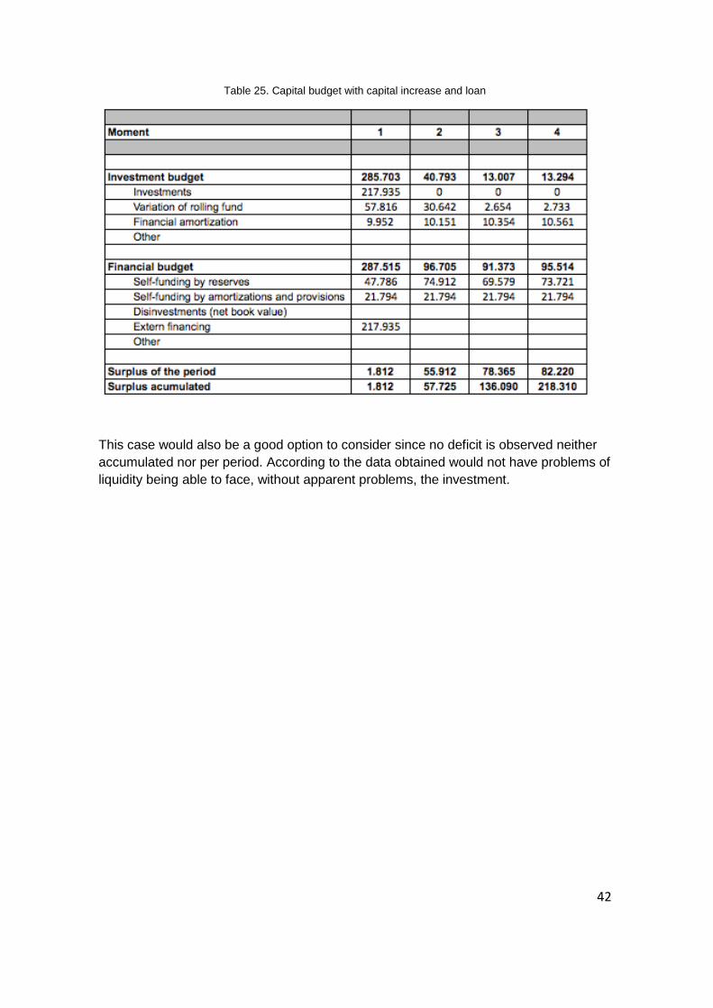
Table 25. Capital budget with capital increase and loan
This case would also be a good option to consider since no deficit is observed neither
accumulated nor per period. According to the data obtained would not have problems of
liquidity being able to face, without apparent problems, the investment.
43
4.3 Choice of the best proposal
In order to know which method is most convenient, different graphs are then plotted to
see the results obtained more clearly.
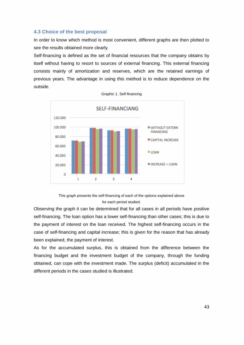
Self-financing is defined as the set of financial resources that the company obtains by
itself without having to resort to sources of external financing. This external financing
consists mainly of amortization and reserves, which are the retained earnings of
previous years. The advantage in using this method is to reduce dependence on the
outside.
Graphic 1. Self-financing
This graph presents the self-financing of each of the options explained above
for each period studied.
Observing the graph it can be determined that for all cases in all periods have positive
self-financing. The loan option has a lower self-financing than other cases; this is due to
the payment of interest on the loan received. The highest self-financing occurs in the
case of self-financing and capital increase; this is given for the reason that has already
been explained, the payment of interest.
As for the accumulated surplus, this is obtained from the difference between the
financing budget and the investment budget of the company, through the funding
obtained, can cope with the investment made. The surplus (deficit) accumulated in the
different periods in the cases studied is illustrated.
44
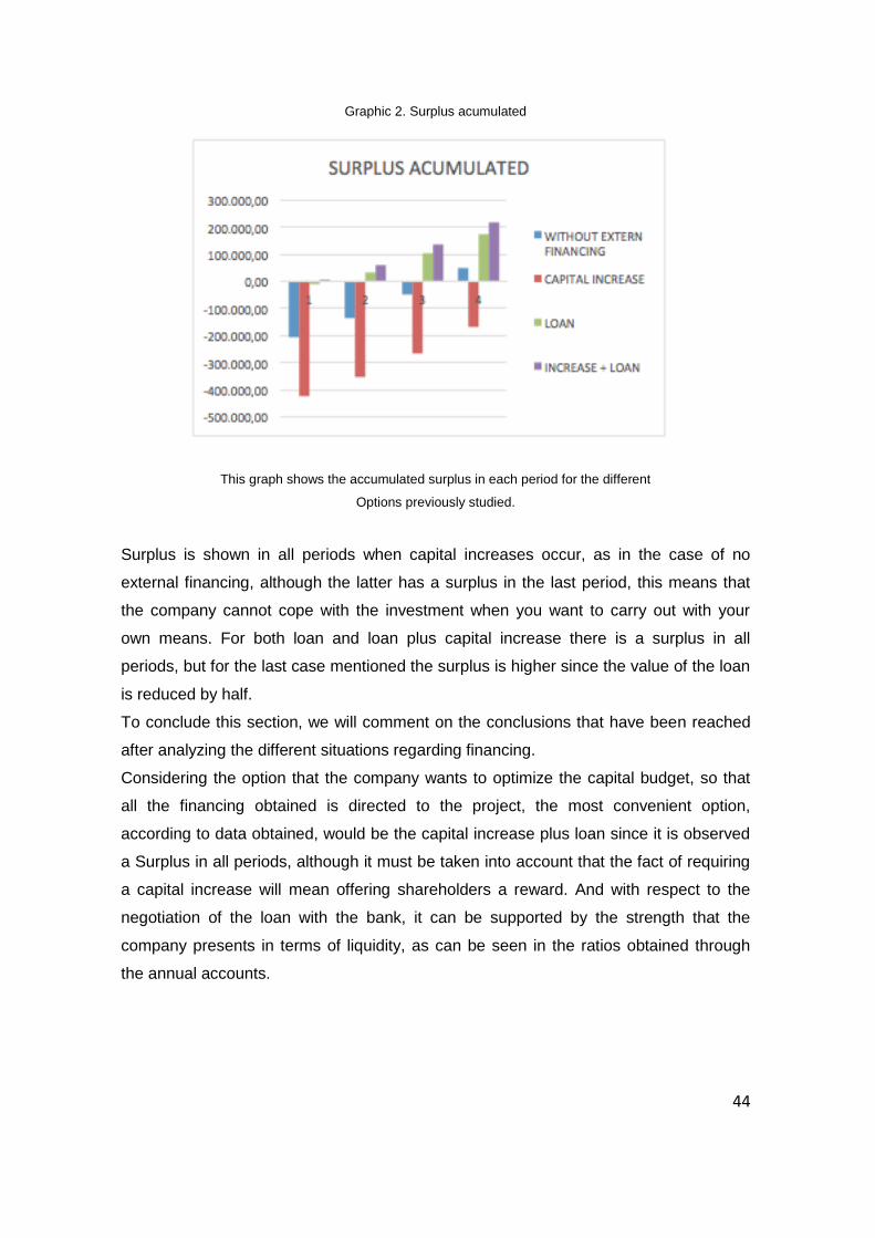
Graphic 2. Surplus acumulated
This graph shows the accumulated surplus in each period for the different
Options previously studied.
Surplus is shown in all periods when capital increases occur, as in the case of no
external financing, although the latter has a surplus in the last period, this means that
the company cannot cope with the investment when you want to carry out with your
own means. For both loan and loan plus capital increase there is a surplus in all
periods, but for the last case mentioned the surplus is higher since the value of the loan
is reduced by half.
To conclude this section, we will comment on the conclusions that have been reached
after analyzing the different situations regarding financing.
Considering the option that the company wants to optimize the capital budget, so that
all the financing obtained is directed to the project, the most convenient option,
according to data obtained, would be the capital increase plus loan since it is observed
a Surplus in all periods, although it must be taken into account that the fact of requiring
a capital increase will mean offering shareholders a reward. And with respect to the
negotiation of the loan with the bank, it can be supported by the strength that the
company presents in terms of liquidity, as can be seen in the ratios obtained through
the annual accounts.
45
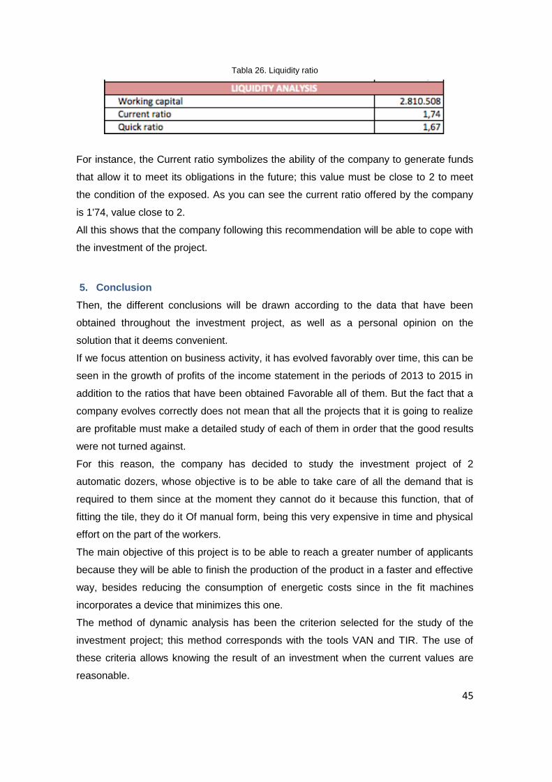
Tabla 26. Liquidity ratio
For instance, the Current ratio symbolizes the ability of the company to generate funds
that allow it to meet its obligations in the future; this value must be close to 2 to meet
the condition of the exposed. As you can see the current ratio offered by the company
is 1'74, value close to 2.
All this shows that the company following this recommendation will be able to cope with
the investment of the project.
5. Conclusion
Then, the different conclusions will be drawn according to the data that have been
obtained throughout the investment project, as well as a personal opinion on the
solution that it deems convenient.
If we focus attention on business activity, it has evolved favorably over time, this can be
seen in the growth of profits of the income statement in the periods of 2013 to 2015 in
addition to the ratios that have been obtained Favorable all of them. But the fact that a
company evolves correctly does not mean that all the projects that it is going to realize
are profitable must make a detailed study of each of them in order that the good results
were not turned against.
For this reason, the company has decided to study the investment project of 2
automatic dozers, whose objective is to be able to take care of all the demand that is
required to them since at the moment they cannot do it because this function, that of
fitting the tile, they do it Of manual form, being this very expensive in time and physical
effort on the part of the workers.
The main objective of this project is to be able to reach a greater number of applicants
because they will be able to finish the production of the product in a faster and effective
way, besides reducing the consumption of energetic costs since in the fit machines
incorporates a device that minimizes this one.
The method of dynamic analysis has been the criterion selected for the study of the
investment project; this method corresponds with the tools VAN and TIR. The use of
these criteria allows knowing the result of an investment when the current values are
reasonable.
46
For the application of the net present value criterion, a discount rate has been
calculated using the CAPM. With this rate the Net Cash Flows that have been obtained
through the difference between the expenses and the future revenues that the company
estimates obtain are deducted.
Analyzed all mentioned aspects and obtained the corresponding results, it is observed
that greater benefits are required to be able to cope with the expenses that the
investment entails. In the situation where the estimated data were the real, the situation
in which it was found is considered unprofitable since the IRR obtained despite being
positive is lower than the discount rate, in addition not enough profits are obtained to be
able to recover in the ten years that the project lasts, the initial investment.
One possible solution to increase this income would be to carry out an effective
publicity campaign with the aim of attracting a larger number of applicants, since it is
not enough to carry out the investment.
As for the financing of the machinery, it will be effective for the company, if it is made
through external financing, shareholders and loan as mentioned in the conclusions of
that point.
In my opinion the dynamic analysis method provides additional information to assess
the risk of the assets to be acquired when it is really difficult to make a prediction about
the rate of depreciation of the investment since the election will always be debatable. In
addition, by homogenizing the net cash flows at the same moment of time, it reduces to
the same unit of measure amounts of money generated at different times of time. I also
consider positive the introduction of net cash flows with negative sign at different times
of the time horizon of the investment without distorting the meaning of the final result.
Despite the results obtained, the company should move forward with the project since,
if this company is currently well positioned in the market, and can do a good advertising
program and reach with it, enough clients to be able to increase the Income, this project
would be beneficial, in addition to contribute to the environment with the fact of wanting
to reduce energy consumption.

47
6. Bibliography
Aragó Manzana, V., Balaguer Franch, M., Cabedo Semper, J., Matallín Sáez, J. and
Soler Domínguez, A. (2012). Dirección financiera. Ed. Low cost books. Valencia.
Brealey, R.A., Myers, S.C., Marcus, A.J. and Mateos-Aparicio, P. (2010) Finanzas
Corporativas. España: Mc Graw Hill.
Mascareñas, J. (2015): El coste del capital. Monografías de Juan Mascareñas sobre
Finanzas Corporativas nº 26. ISSN: 1988-1878. Disponible en:
http://www.juanmascarenas.eu/monograf.htm.
Damodaran, A. (2013) Equity Risk Premiums (ERP): Determinants, Estimation and
Implications – The 2013 Edition (March 23, 2013). Disponible en; SSRN:
http://ssrn.com/abstract=2238064 or http://dx.doi.org/10.2139/ssrn.2238064
Bolsas y mercados españoles. Clasificación sectorial bursátil descripción general y
especificaciones pos subsector, 2015. Disponible en:
http://www.bolsamadrid.es/docs/Acciones/sect.pdf
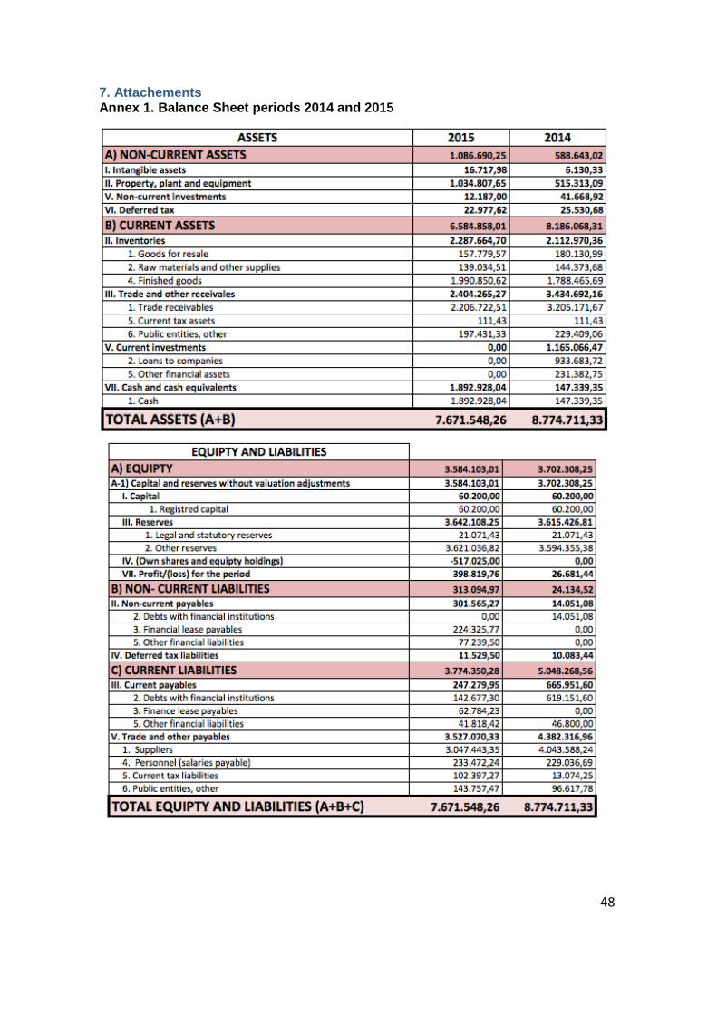
48
7. Attachements Annex 1. Balance Sheet periods 2014 and 2015
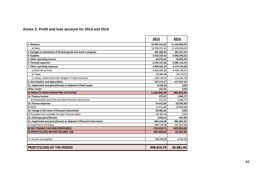
49
Annex 2. Profit and loss account for 2014 and 2015

50
Annex 3. Net Cash Flows
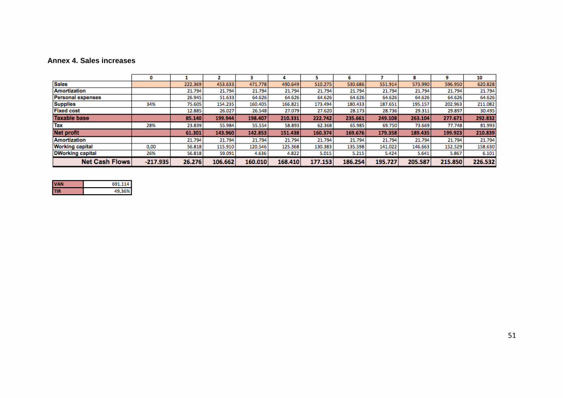
51
Annex 4. Sales increases
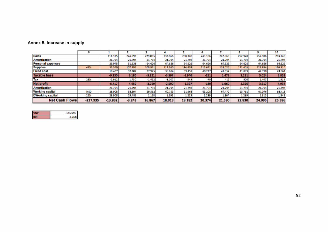
52
Annex 5. Increase in supply
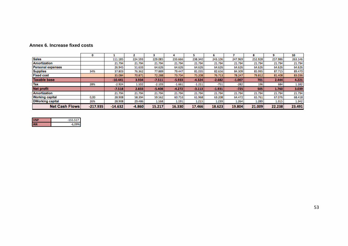
53
Annex 6. Increase fixed costs
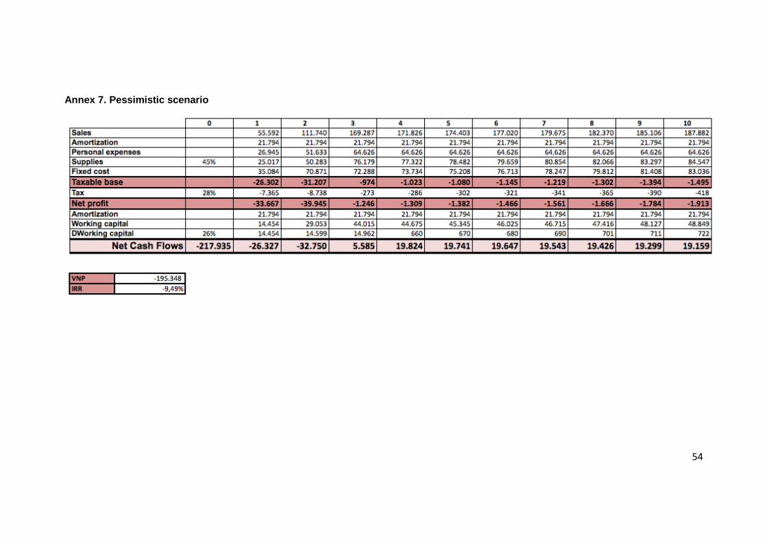
54
Annex 7. Pessimistic scenario
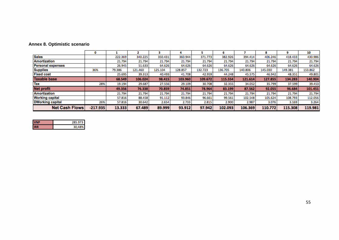
55
Annex 8. Optimistic scenario
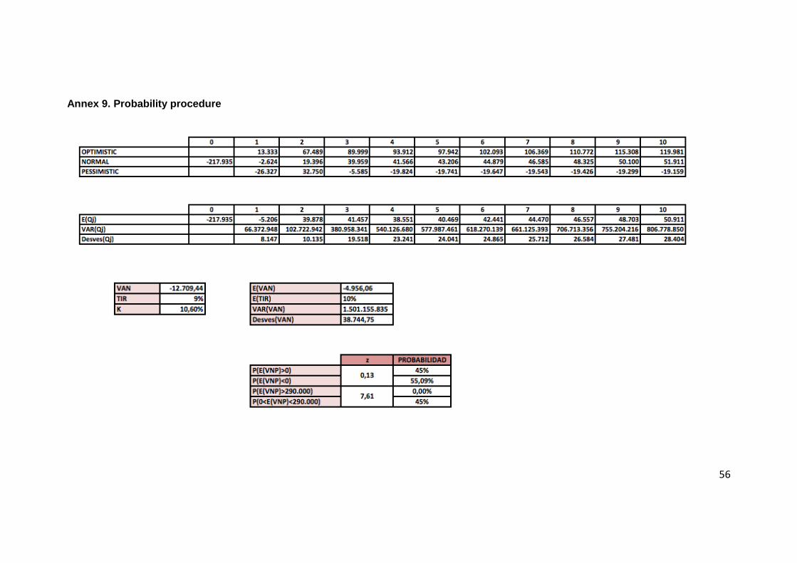
56
Annex 9. Probability procedure