Embed Size (px)
Citation preview
Economic and Environmental Impacts of Collecting Waste Cooking Oil for use as Biodiesel under a Localized Strategy
BY CHRISTOPHER R. WOOD
A THESIS SUBMITTED IN PARTIAL FULFILLMENT OF THE REQUIREMENTS FOR THE MASTER OF SCIENCE DEGREE IN
INDUSTRIAL AND SYSTEMS ENGINEERING IN KATE GLEASON COLLEGE OF ENGINEERING OF
ROCHESTER INSTITUTE OF TECHNOLOGY
INDUSTRIAL AND SYSTEMS ENGINEERING DEPARTMENT ROCHESTER INSTITUTE OF TECHNOLOGY
ROCHESTER, NEW YORK
OCTOBER 2007
COMMITTEE MEMBERS DR. ANDRES CARRANO DR. BRIAN THORN ASSOCIATE PROFESSOR ASSOCIATE PROFESSOR INDUSTRIAL AND SYSTEMS ENGINEERING INDUSTRIAL AND SYSTEMS ENGINEERING ROCHESTER INSTITUTE OF TECHNOLOGY ROCHESTER INSTITUTE OF TECHNOLOGY

KATE GLEASON COLLEGE OF ENGINEERING
ROCHESTER INSTITUTE OF TECHNOLOGY
ROCHESTER, NEW YORK
CERTIFICATE OF APPROVAL
MASTER OF SCIENCE DEGREE THESIS
The M.S. Degree Thesis of Christopher R. Wood has been examined and approved by the thesis committee
as satisfactory for the thesis requirement for the Master of Science degree
Dr. Andres Carrano, Ph.D. Advisor
Dr. Brian Thorn, Ph.D. Advisor
1

Abstract Some of the vital aspects in the diffusion of renewable energies are the cost of producing
the energy, as well as the environmental impacts associated with its lifecycle. As
petroleum based energy becomes increasingly costly, alternatives will be relied upon to
meet the ever increasing energy demand. Biofuels, and biodiesel in particular, could be a
near term solution for providing a transitional fuel to meet the energy demand of the
transportation sector. However, the costs of biodiesel, as well as perceptions of a negative
energy balance are hindering its widespread adoption. Using waste cooking oil (WCO)
can reduce the cost of raw materials necessary for producing biodiesel, when compared to
traditional sources, and by collecting and using biodiesel locally, its cost can be further
reduced. This research involves the design and development of a simulation model to
analyze the costs and emissions associated with waste cooking oil collection for the local,
or decentralized, production and use of biodiesel. A case study for the food and beverage
industry is investigated. A series of simulation experiments was used to evaluate different
scenarios for utilizing the unexploited capacity of a local food and beverage distribution
network for the collection of waste cooking oils. The economic and environmental costs
associated with collecting WCO were compared to the economic and environmental
savings from using biodiesel, the impacts of such operation upon service level are also
investigated. Based on the local food and beverage network used to construct the model
parameters, biodiesel production from WCO on a localized scale has positive impacts to
both cost and emissions without sacrificing customer service.
2

Table of Contents 1. Introduction ..................................................................................................................... 7
1.1 Implications of Waste ............................................................................................... 8 1.2 Implications of Energy Use ...................................................................................... 9
2. Problem Statement ........................................................................................................ 11 3. Literature Review .......................................................................................................... 15
3.1 Waste Cooking Oil Resources in the USA ............................................................. 15 3.2 Biodiesel production ............................................................................................... 16 3.3 Waste Management ................................................................................................. 18
4. Scope and Methodology ............................................................................................... 20 4.1 Overview of Model ................................................................................................. 20 4.2 Simulation Model.................................................................................................... 24 4.3 Verification and Validation..................................................................................... 41 4.4 Experimental Design ............................................................................................... 42
5. Full Piggy Back System Results ................................................................................... 47 5.1 Full Piggy Back System Results for Emissions Savings ........................................ 48 5.2 Full Piggy Back System Results for Cost and Service Level ................................. 59 5.3 Effects to the Full Piggy Back System from Changes in Total Number of Stops .. 65
6. Hybrid Piggy Back System Results .............................................................................. 68 6.1 Hybrid Piggy Back System Emissions Results ....................................................... 68 6.2 Hybrid Piggy Back System Results for Cost .......................................................... 74
7. Conclusions ................................................................................................................... 88 8. Future Work .................................................................................................................. 91 9. Bibliography ................................................................................................................. 93 Appendix A. Simulation Code: SIMAN ........................................................................... 97
3

List of Figures
Figure 1. Full Piggy Back System .................................................................................... 21 Figure 2. Hybrid Piggy Back System ............................................................................... 22 Figure 3. GUI at model start ............................................................................................. 25 Figure 4. Model Start ........................................................................................................ 26 Figure 5. Route and Emissions Variable and Attribute Initialization Modules ................ 27 Figure 6. Stop Type 1 and Stop Type 2 Creation ............................................................. 29 Figure 7. Stop Type 3 Creation and Route to Dispatch Station ........................................ 30 Figure 8. Dispatch Section ................................................................................................ 31 Figure 9. Delivery and Pickup Stop (Stop Type 1) ........................................................... 34 Figure 10. Delivery only Stop (Stop Type 2) ................................................................... 34 Figure 11. Pickup Only Stop (Stop Type 3) ..................................................................... 35 Figure 12. Warehouse Station ........................................................................................... 36 Figure 13. Refueling and Cost Calculation Station .......................................................... 36 Figure 14. Emissions Calculations .................................................................................... 39 Figure 15. Reporting Section ............................................................................................ 41 Figure 16. Main effects plot for CO Savings (2 )2
8-3 ......................................................... 52 Figure 17. Pareto of Main Effects Response Values for CO Savings2 ............................. 52 Figure 18. Interaction effects plot for CO2 Savings (28-3) .............................................. 53 Figure 19. Pareto Chart of the Standardized effects for CO2 savings .............................. 54 Figure 21. Interaction effects plot for CO Savings (2 )2
6-1 ................................................ 55 Figure 22. CO Savings Vs Number of Stops Generating WCO out of 15 Total Stops2 .. 56 Figure 23. CO and THC Savings Vs Number of Stops Generating WCO out of 15 Total Stops .................................................................................................................................. 57 Figure 24. NO Savings Vs Number of Stops Generating WCO out of 15 Total StopsX .. 58 Figure 25. Main effects plot for cost (2 )8-3 ....................................................................... 62 Figure 26. Pareto of Main Effects Response Values for Cost .......................................... 62 Figure 27. Interaction effects plot for Cost (2 )8-3 .............................................................. 63 Figure 28. Cost Vs Number of Stops Generating WCO out of 15 Total Stops ................ 64 Figure 29. Service Level Vs Number of Stops Generating WCO out of 15 Total Stops . 64 Figure 30. Response Plot for Cost and CO Savings VS Density of Stops with WCO for 10 Total Stops
2 ................................................................................................................... 66
Figure 31. Response Plot for Cost and CO Savings VS Density of Stops with WCO for 30 Total Stops
2 ................................................................................................................... 66
Figure 32. Actual Total Distance (Local Distributor) VS Number of Stops .................... 67 Figure 33. Main Effects plots for CO Savings (2 )2
10-5 ..................................................... 70 Figure 34. Pareto of Main Effects Response Values for CO Savings2 ............................. 71 Figure 35. Pareto Chart of the Standardized Effects for CO Savings (2 )2
5 ...................... 73 Figure 36. Main Effects plots for CO2 Savings (25) ........................................................ 73 Figure 37. Interaction Effects plots for CO Savings (2 )2
5 ................................................ 74 Figure 38. Main Effects plots for Cost (2 )10-5 ................................................................... 76 Figure 39. Pareto Chart of the Standardized Effects for Cost (2 )8-3 ................................. 79 Figure 40. Hybrid Piggy Back System Main Effects Plots for Cost (2 )8-3 ....................... 79 Figure 41. Hybrid Piggy Back System Interaction Effects plots for Cost (2 )8-3 ............... 80
4

Figure 42. 3-D Response Surface for Cost Vs Additional Non-Customer Stops Vs Additional Travel Distance per Additional Stop .............................................................. 82 Figure 43. CO Savings versus Additional Non-Customer Stops Vs Additional Travel Distance per Additional Stop
2 ............................................................................................ 83
Figure 44. CO Savings versus Additional Non-Customer Stops Vs Additional Travel Distance per Additional Stop ............................................................................................ 84 Figure 45. THC Savings versus Additional Non-Customer Stops Vs Additional Travel Distance per Additional Stop ............................................................................................ 85 Figure 46. NO Savings versus Additional Non-Customer Stops Vs Additional Travel Distance per Additional Stop
X ............................................................................................ 86
Figure 47. Service Level versus Additional Non-Customer Stops Vs Additional Travel Distance per Additional Stop ............................................................................................ 88
5

List of Tables Table 1. Truck Specifications ........................................................................................... 27 Table 2. Sample Stop Location and Stop Type Array ...................................................... 30 Table 3. Factors and Their Corresponding Baseline Values for the Full and Hybrid Piggy Back Scenarios .................................................................................................................. 45 Table 4. Experimental Design Factors .............................................................................. 45 Table 5. Aliasing Structure for 2 Fractional Factorial Design8-3 ...................................... 46 Table 6. Aliasing Structure for 2 Fractional Factorial Design10-5 ..................................... 46 Table 7. Full Piggy Back System ANOVA for CO Saving (2 )2
8-3 ................................... 48 Table 8. Full Piggy Back System ANOVA for Cost (2 )8-3 ............................................... 48 Table 9. Aliasing Structure for 2 Fractional Factorial Design6-1 ....................................... 50 Table 10. Estimates Effects and Coefficients for CO2 Savings (2 )8-3 .............................. 51 Table 11. Estimates Effects and Coefficients for CO Savings (2 )2
6-1 .............................. 53 Table 12. Estimates Effects and Coefficients for Cost (2 )8-3 ............................................ 61 Table 13. Hybrid Piggy Back System ANOVA Table for CO Saving (2 )2
10-5 ................. 68 Table 14. Hybrid Piggy Back System ANOVA Table for Cost (2 )10-5 ............................. 68 Table 15. Estimates Effects and Coefficients for CO Savings (2 )2
10-5 ............................. 69 Table 16. Hybrid Piggy Back System ANOVA for CO Saving (2 )2
5 .............................. 72 Table 17. Estimates Effects and Coefficients for CO Savings (2 )2
5 ................................. 72 Table 18. Estimates Effects and Coefficients for Cost (2 )10-5 ........................................... 75 Table 19. Hybrid Piggy Back System ANOVA Table for Cost (2 )8-3 .............................. 77 Table 20. Hybrid Piggy Back System Estimated Effects and Coefficients for Cost (2 )8-3 78 Table 21. Maximum Deviation Distances for Cost, CO, THC, CO , and NO2 X ............... 90
6

1. Introduction Sustainable development has been defined as development that meets the needs of the
present without compromising the ability of future generation to meet their own needs
(WCED, 1987.) It is common knowledge that our natural resources are decreasing while
waste production is increasing. These trends have spurred regulations on emissions,
waste, and energy. As more regulations are set in place, higher cost will be associated
with compliance to the regulations unless strategies to mitigate the costs in a sustainable
manner are developed.
Sustainable development and industrial ecology are key to complying with energy and
environmental regulations in a cost effective manner. Industrial ecology is defined as the
shifting of industrial process from open loop systems, in which resource and capital
investments move through the system to become waste, to a closed loop system where
wastes become inputs for new processes (Wikipedia, 2006). By closing these industrial
loops, natural resource consumption will be reduced through the extraction of value from
waste. In essence, waste from one industry will be the feedstock for another therein
reducing the amount of raw material necessary to accomplish the same functionality.
Energy, material, waste, and emissions are the principle inputs and outputs from every
process from manufacturing through the service industries. Energy is required to
manipulate the system, while waste and emissions will be generated due to inefficiencies
in that system. According to the Energy Information Agency (2005), world energy
consumption has been increasing at a significant rate with 2003 world consumption
amounting to 421 Quadrillion Btus. It is also predicted that global energy demand will
double by 2050 (DOE, 2006). On the other hand, the Environmental Protection Agency
7

reports that the USA generated around 235.5 million tons of municipal solid waste in
2002 (EPA, 2003). Energy production and use and waste are also the largest producers of
CO2 and methane respectively in the USA (EPA, Global Warming, 2006.). These gases
are both considered greenhouse gases.
Parallel to the trends in energy consumption and waste generation, the cost associated
with them is increasing. Energy prices are rising and will continue to do so with reduced
supplies of fossil fuels. The cost of waste disposal is also increasing as landfill space
becomes limited and the logistics associated with its removal become more difficult.
1.1 Implications of Waste
Landfills are the largest producers of anthropogenic methane in the USA at 55.8 million
metric tonnes of CO2 equivalents in 1998. This represents 61% of all solid waste
emissions (Waste, 2006.). Landfills also require vast land to accommodate such high
volumes of waste and are known to leach harmful chemicals to ground water sources.
These leached contaminants pose threats to soil and drinking water sources.
In addition to polluting the environment, landfilled waste contains inherent material and
energy value that is lost. This waste material and energy could be utilized instead of
harvesting new materials to provide the same function. By closing the material loop
energy and resources can be conserved.
In order to reduce environmental impacts and resource use, waste materials that are
typically land filled need to be analyzed to determine feasible reuse applications. The
reuse strategy for waste could be as a material feedstock or an energy source depending
on the characteristics of the substance.
8

1.2 Implications of Energy Use
Energy production has primarily been based upon the combustion of fossil fuels such as
oil and coal. These resources are finite, and pose significant environmental impact from
their combustion. While coal is predicted to be a viable energy resource for 90 - 200
years, it has been predicted that the world oil supply is reaching its peak (Energy
Information Agency, 2005). Oil is the leading energy source for the transportation sector
behind electricity production (Energy and Emissions -EPA). As oil is consumed it will
gradually rise in price as supply drops, extraction becomes more difficult, and demand
rises. With an increase in price and decrease of supply, consumers will look for more
economical methods to provide energy for transportation.
The environmental impact associated with fossil fuel use is another issue concerning its
longevity as a sustainable energy resource. The combustion of fossil fuels generates
emissions harmful to human health and the environment. Greenhouse gases (GHG) are
emitted more from the combustion of fossil fuels than from any other source. According
to National Academy of Sciences (2006) anthropogenic GHG emissions are contributing
to global warming and have aided in rising global temperature by 1.4 degrees Fahrenheit.
Emissions associated with fossil fuel combustion include carbon monoxide, carbon
dioxide, nitrogen oxides, sulfur dioxide, particulate matter, and volatile organic
compounds. These pollutants cause a number of harmful impacts such as respiratory
problems and the acidification of fresh water sources.
Within the energy sector, electricity production and transportation are the largest
consumers of fossil fuels therefore the largest producers of emissions. The transportation
industry is dominated by petroleum as an energy provider due to its transportability and
9

compatibility with current propulsion technology. According to the Energy Information
Agency (2005) petroleum is approaching its peak production output. With dwindling
supplies, petroleum will gradually lose the ability to fuel the transportation sector
Alternatives need to be evaluated to determine viable options for transitioning to a new
transportation fuel base. This transition may not be provided by a single fuel source or be
provided on a national scale as petroleum fuel is today. The transportation industry may
need to be based on several fuel sources requiring different production, propulsion, and
refueling technologies such as hydrogen, ethanol, and biodiesel.
For all the reasons stated above, the use of petroleum based fuels for transportation
presents a challenge to sustaining mobility, the environment, and human health.
Alternatives to oil need to be analyzed to determine a more sustainable solution.
Alternatives have been developed such as hydrogen and biofules, however their wide
scale adoption has been hindered. One of the major setbacks to these alternatives is cost.
For example, hydrogen and fuel cells for vehicles and the infrastructural requirement to
supply it are too expensive with current technology, thus not commercially viable.
Nevertheless, there are solutions that can compete with the traditional transportation
energy and waste methods in terms of economics and also provide external benefits to the
environment and human health.
There are transportation fuel alternatives that do not require new infrastructures.
Biodiesel is a fuel that can be blended into regular diesel, or used on its own in order to
reduce the rate at which petroleum based fuel is consumed. This reduction in the
consumption rate can allow for more time to study alternative fuel sources and
technology while reducing emissions associated with the transportation industry.
10

Biodiesel is a renewable, carbon neutral, fuel that can reduce the dependence of fossil
fuels in the transportation sector especially from heavy duty vehicles. Carbon neutral
refers to a system that neither produces nor eliminates carbon in the atmosphere,
therefore not affecting global warming. However, widespread adoption of biodiesel is
hindered by the cost and difficulty of raw material acquisition. Typically biodiesel is
produced from virgin agricultural based oil such as soy or rapeseed oil, however many
vegetable based oils will work. Virgin agricultural based oil costs roughly $0.53/liter and
the conversion to biodiesel another $0.15/liter (Haas, 2005). These combined costs
exceed the cost of petroleum derived diesel before profit mark-up or federal taxes are
included. In order to make biodiesel viable, methods for cost reduction must be
employed. A current method for reducing cost is through the use of waste cooking oil
(WCO) as a cheap feedstock for production (Supple et al., 1999).
In 1998 the US Department of Energy National Renewable Energy Laboratory
determined that each restaurant produces an average range of 6,268 - 9,453 lbs (3250 –
4875 liters) of WCO per year (Wiltsee,1998). Based on these numbers the national
production of WCO with a population of 295 million is between 2.6 – 3.9 billion gallons
a year. This is equivalent to 6.1 – 9.2% of the total US diesel use for the transportation
sector in according to the Energy Information Agency (2005).
2. Problem Statement
With the current trend of increasing energy costs, businesses are experiencing higher
operational costs. Companies with transportation fleets, such as distributors, have been
impacted by the increase in fuel cost. As a result, these companies have to either absorb
11

these costs through profit reductions, or pass the cost on to their customers. The cost of
energy will continue to rise with the increasing demand for petroleum fuels. Therefore,
the cost of goods and services will continue to increase as well. In addition to increased
costs, the use of petroleum fuels produce harmful emissions, such as CO2 and particulate
matter, and creates a reliance on foreign nations for energy.
Waste generation has also become an issue in terms of cost, land use, and soil and water
contamination. Companies that produce waste material are required to dispose of these
wastes in an appropriate manner. The disposal of waste costs money for pick-up,
transport, and treatment method. These disposal costs can go straight to the bottom line
increasing operations cost of restaurants. Once the waste has been disposed of, there is
the possibility that it can contaminate local soil and water. Finally, the transportation
associated with collecting the waste creates harmful emissions through the combustion of
petroleum fuels.
In some cases waste is capable of providing energy through either direct use or
conversion processes. In other words, the waste being generated from one system can be
returned back into another system as fuel. For example, waste cooking oil can be
converted to biodiesel for use in the transportation sector.
The major hurdle to overcome with waste oil based production of biodiesel is finding a
reliable and economically feasible supply. This problem seems to be aggravated by the
need for very large quantities of WCO required for operating national scale production
facilities. To accommodate such high volumes, large cost would be incurred in the
development of a collection infrastructure. Local and decentralized alternatives need to
12

be addressed to determine if there is a possibility for an industry to use its current
distribution infrastructure and operations to recover and use the WCO.
The food and beverage (F&B) distribution industry has a unique possibility to recover
WCO without having to develop a new infrastructure. In this case, the F&B distribution
industry already have the infrastructure in place. The WCO that is produced by
restaurants, the customers of the F&B distribution industry, can be collected and
converted to biodiesel for use in the trucks that are delivering the food or beverages. This
local and decentralized system may be more feasible than dedicating an entire vehicle
fleet to recover WCO under a national centralized strategy. By collecting the WCO for
use as biodiesel a material loop can be closed.
In the case of F&B distributors there is an opportunity to reduce emissions, the
dependence on foreign oil, waste generation, and operations costs for themselves and
their customers. This opportunity lies in 2 distinct areas. First, the F&B distribution
industry can utilize a current waste stream, waste cooking oil, produced by restaurants as
a fuel source, and secondly this can eliminate the need for a waste collection service to
dedicate trucks for recovering the waste. There is an incentive for the restaurants to give
the WCO to the distributor for free. Currently restaurants pay for the removal of their
WCO, therefore they would likely appreciate a free removal service provided from one of
their suppliers. This could also be a strategy to gain customers for a F&B distributor who
wants to expand their share of the market.
The aim of this thesis will be to investigate a F&B distribution network that includes the
recovery of WCO, the production of WCO to biodiesel, and the use of the biodiesel in the
trucks that are making the deliveries. The analysis will address cost implications
13

associated with the added time and distance to pick-up the WCO and use biodiesel.
Emissions changes through the use of biodiesel versus petroleum based diesel will also
be determined. The ability to meet the core business demands with increased services will
also be investigated.
14

3. Literature Review Biodiesel from different feedstocks has been researched thoroughly in terms of processes,
costs, and emissions that arise throughout its production and use phases (Haas, 2005,
Graboski, 1998). Models have been built to understand municipal solid wastes (MSW)
logistical issues. Other research has been conducted to understand simultaneous pick –up
and delivery logistics; and the quantities of WCO produced in the USA has been
determined. However, no studies have brought these ideas together to examine the
logistics of WCO as the raw material for biodiesel production and use under a
decentralized scenario.
3.1 Waste Cooking Oil Resources in the USA There have been a number of studies conducted to determine the quantity of WCO
produced per year nationally or per restaurant. In 1998 the US Department of Energy’s
National Renewable Energy Laboratories (NREL) conducted a waste grease resource
study of 30 metropolitan cities in the US. This study indicated little variability between
the number of restaurants per 1000 people in urban areas with a range of 1 to 2
restaurants/1000 people and a weighted average of 1.41. The NREL study also concluded
that each restaurant produces a weighted average range of 6,268 - 9,453 pounds (3250 –
4875 liters) of WCO per year (Wiltsee, 1998). Based on these numbers the national
production of WCO with a population of 295 million is between 2.61 – 3.94 billion
gallons a year. This is equivalent to 6.1 – 9.2% of the total US diesel use for the
transportation sector in 2004 (Energy Information Agency, 2005)
15

The Minnesota Department of Agriculture also conducted a study to determine the
quantity of WCO produced per year in the USA. This study concluded that between the
years of 1995 and 2001 the average production of WCO was 2.63 billion gallons
(Groschen, 2002). All of the studies reported the possible quantities of WCO that could
be recovered, but none looked into the feasibility of physically collecting it.
3.2 Biodiesel production Currently the two most common processes to produce biodiesel are by way of an alkali-
catalyst system or an acid-catalyst system. Both systems are known as transesterification
processes. These two methods have different strengths and weaknesses based upon the oil
feedstock used to produce the biodiesel. The alkali-catalyst method is better suited for
virgin oils, due to it inability to break down the high content of free fatty acids in waste
oils, and has a faster processing time. These characteristics have made it the most
predominantly used in biodiesel production processes. The acid-catalyst method is better
suited for producing biodiesel from WCO, but requires longer processing times. When
using WCO in the alkali process, a pretreatment step is required to remove the high
content of free fatty acids from the waste oil. This added equipment increases the cost of
the setup and increases the processing time. It has also been reported that 70-95% of
biodiesel production cost arise from the raw material cost (Krawczyk, 1996; Connemann
and Fischer, 1998), therefore causing virgin oil based biodiesel production costs to be
much higher than waste oil based biodiesel. This figure highlights a need to use waste
oils in the production of biodiesel based on the impacts to cost.
The alkali-catalyst process has been studied in laboratories to determine optimum process
parameters (Freedman et al., 1984; Noureddini and Zhu, 1997; Darnoko and Cheryan,
16

2000). Industrial scale production alkali-catalyst processing was demonstrated in 1984 by
Kreutzer and has been studied further since then (Krawczyk, 1996; Connemann and
Fischer, 1998). It was also determined that the alkali-catalyst system could only work
with oils with low fatty acid content, hindering its ability to produce biodiesel from waste
WCO with out a pretreatment step (Freedman et al., 1984; Jeromin et al., 1987). The
pretreatment step, esterification, was identified and introduced by Lepper and Frienhagen
(1986).
The acid catalyst process has only been demonstrated at the bench scale, even though it is
robust to different feedstock oils in terms of their free fatty acid content. Acid-catalyst
transesterification was explored by Freedman et al. (1984) to determine operating
parameters. Canakci and Gerpen (2001) investigated the acid-catalyst process to
understand the effects of different operating parameters on the conversion percentages
from oil to biodiesel. The parameters were examined independently so no optimal
solutions were recommended. WCO was converted to biodiesel using the acid-catalyst
process in a laboratory by Ripmeester (1998) and Mcbride (1999). It has been shown that
the acid-catalyst process is advantageous when creating biodiesel from WCO, because
there is no pretreatment step required (Zyang et al., 2003).
The economics of biodiesel production using both the alkali and acid catalyst methods
were compared to determine the pros and cons of each using different feedstock oils in
terms of their process technology (Zhang, Et al. 2003). Each process was compared using
both virgin oils and waste oils. It was determined that the alkali-catalyst process using
virgin oil had the lowest fixed capital cost, but the acid-catalyst process using WCO was
the most economically feasible. The acid-catalyst process had the lower total
17

manufacturing cost, a greater after tax rate of return, and a lower biodiesel break even
price. Zyang et al. (2003) showed that biodiesel production from WCO using the acid-
catalyst process is a potentially competitive alternative to the commonly used alkali-
catalyst process using virgin oils.
These findings show that the use of waste oils can have a beneficial impact on the cost of
biodiesel production. The findings also highlight a waste product that can be diverted
from the waste stream and cascaded into another use. These reports do not however state
an economically feasible way of collecting the waste material for use in the production of
biodiesel.
3.3 Waste Management Waste management has been researched with respect to its supply chain using various
techniques under a vast array of scenarios. The economic and environmental performance
have been taken in to account, however the methods have not provided a technique for
modeling decentralized collection of waste for use as fuel in the distribution industry. The
major research in waste management has been focused on understanding and optimizing
centralized or large scale waste issues. In order to understand waste management, the rate
at which waste is generated was determined (Hockett et al., 1995; Chen and Chang, 200).
Once the generation levels were understood optimum treatment locations were
established (Huang et al., 1995; Chang and Wang, 1996; Fredriksson, 2000) to manage
the wastes using different treatment methods such as landfilling, recycling, and
incineration (Huhtala, 1997; Dalemo et al., 1998; Highfill and McAsey, 2001).
Other research looked into the environmental and social impacts associated with waste
management systems (Nixon et al., 1997; Slater and Frederiksson, 2001; Powell, 1996).
18

Life cycle inventories have been built around the different waste management treatment
scenarios mostly based on the work done by White et al. (1999). Some models also
included a life cycle analysis to determine the impacts associated with the system (Munda
and Romo, 2001). The economics of municipal solid waste systems has also been
considered when making decisions on which treatment method and/or collection scenario
should be chosen (Morris and Holthausen, 1994; Jenkins et al., 2000; Palmer et al., 1997;
Fullerton and Wu, 1998; Hong, 1999).
These studies analyzed centralized, regional scale collection and treatment scenarios for
municipal solid waste (MSW) without looking into the holistic approach of utilizing
specific waste streams directly as feedstocks for other systems. These methods also
neglect the local decentralized approach to waste management such as collecting waste
for local reuse.
19
4. Scope and Methodology
The objective of this study is to analyze the parameters that affect the collection of WCO
for use as biodiesel, on a decentralized scale, in terms of economics and the environment.
In order to analyze the key factors, a simulation model was built to represent two
scenarios under which this system can take place. This model was flexed under different
experimental conditions to understand the systems dynamics.
4.1 Overview of Model The simulation model represents a single truck within an F&B distribution system that
has a variable number of customers and distances between those customers. The
customers will produce different quantities of WCO, and will be supplied different
amounts of products freeing up space in the truck for the WCO to be collected. Once the
truck has visited all the required stops, it will return to the warehouse where the WCO
and any remaining product will be offloaded. The WCO will then be traded to a local
biodiesel producer for biodiesel at a reduced price. Once the first batch of WCO has been
traded the truck will be filled with a mix of biodiesel and petroleum based diesel. The
costs of collecting the WCO will be calculated dynamically, while the saving from the
use of biodiesel will also be tracked. During the simulation, emissions savings from the
biodiesel use will be updated for each route.
Two scenarios will be explored, the first model scenario will represent a current state
F&B distribution system that only recovers WCO from restaurants who are already being
supplied. This system will be referred to as the full piggy backed system (See Figure 1).
This model was run with out picking up WCO in order to set a baseline for comparison.
20

The second scenario, to be referred to as the hybrid piggy back system was constructed
similar to the first scenario, except WCO could also be recovered from restaurants that
are not currently customers of the distribution company (See Figure 2). In the hybrid
piggy back model the extra distance traveled will result in added emissions and costs,
therefore those emissions and cost will be estimated to determine if the added distance
traveled was worth while in terms of its environmental and economic impact.
Figure 1. Full Piggy Back System
21
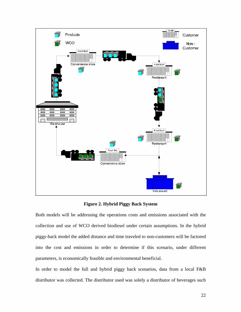
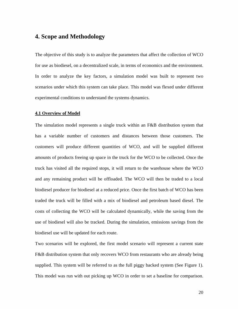
Figure 2. Hybrid Piggy Back System
Both models will be addressing the operations costs and emissions associated with the
collection and use of WCO derived biodiesel under certain assumptions. In the hybrid
piggy-back model the added distance and time traveled to non-customers will be factored
into the cost and emissions in order to determine if this scenario, under different
parameters, is economically feasible and environmental beneficial.
In order to model the full and hybrid piggy back scenarios, data from a local F&B
distributor was collected. The distributor used was solely a distributor of beverages such
22

as beer, energy drinks, and soda. The data collected from the local distributor was used to
build the model to closely represent how the system actually works. Data on WCO
production at restaurants was obtained from literature (Wiltsee, 1998).
Routing sheets containing information on distance, time, number of stops, average loads
were obtained from the local distributor. The routing sheets were the basis for the
assumptions built into the model and are as follows:
• Fuel consumption and emissions will not change based upon the load of the truck
• Every stop is visited one time per week
• Every route has 15 stops
• The cost of labor (Truck Driver) is $25 per hour
• All WCO collected will be converted to biodiesel at a 90% conversion factor
• All produced biodiesl will be used in the distribution fleet or traded for equal
value
• All WCO collected will come in 5 gallon drums (partially full is allowed)
• The average speed of the truck is 35 MPH
• The cargo capacity of the truck is 567000 in3
• The truck has a 277 HP diesel motor
• The average fuel economy of the truck is 6 MPG
• The fuel capacity of the truck is 100 gallons
23

4.2 Simulation Model
The model was built using the Arena 7.01 software package. Other tools such as linear
programming were considered and evaluated, however Arena was chosen based on the
ability to accommodate for the high levels of variability with in the system. Arena also
allows for quick manipulation of the parameters in the model to aid in the
experimentation process. Finally, the problem being investigated could be looked at for
many different location in the future, so the ability to quickly change parameters through
a graphical user interface makes Arena a good long term tool to build upon for future
research purposes. The ability to easily change the variability within the system is useful
when modeling the recovery of WCO for use as biodiesel due to the fact that the
distances traveled, packing percent of the vehicle at route start, the amounts of WCO at
each stop, and the volume of products dropped at each stop are variables that could be
different for each system. The model can be customized to represent an exact scenario, or
it can be run under different parameters to create a heuristic for the best cases in which
F&B distributors should collect WCO for use as biodiesel. This approach and the idea of
further studies of distribution systems is made easy with a package such as Arena.
A graphical user interface (GUI) was constructed to allow the modeler to set the
parameters for different runs of the model (See Figure 3). The parameters that can be
manipulated by the modeler from the GUI include the number of routes to be made per
replication, the number of customers who have WCO, the number of customer who do
not have WCO, the additional distance traveled to go to non-customers, the number of
non customers that will be visited, the hybrid (1) or full piggy back(0) scenario, the cost
24

of diesel, the cost of biodiesel, the percentage of biodiesel to be mixed with the regular
diesel, and the time the truck is delayed at each stop during the pick-up process. Once the
parameters have been entered by the modeler the run button is clicked to begin the
simulation.
Figure 3. GUI at model start The simulation model can be broken into five functional sections, truck and route
creation, dispatching, stops, warehouse, and reporting. These functional sections can be
further reduced to more detailed stations. The truck and route creation section can be
divided into model start, route set-up, and refueling and cost calculation. The dispatching
section has no further breakdown. The stops section can be broken into three different
stop types, customer delivery and WCO pick up (Stop type 1), customer delivery only
(Stop type 2), and non-customer WCO pick-up only (Stop type 3). The warehouse section
can be divided into biodiesel production and emissions calculations. The reporting
section is stand alone like the dispatching section.
In the truck and route creation section, the first station, model start, includes the creation
of the truck, truck and model variable assignment, and an entity separation module. The
25

entity separation module duplicates the truck entity, allowing for two sets of logic to be
completed simultaneously. The duplicated entity is sent to keep track of cost and fuel
while the original entity is used to complete the routes (See figure 4).
Create TruckVariables
Truck and GlobalControl Entity
Create Refueling
0
0
0
Figure 4. Model Start In the first module of model start, one entity is created using the create module to
represent the truck. The truck entity then moves to an assign module where the truck
specifications of cargo capacity, fuel capacity, fuel economy, and horsepower, are
assigned to that truck as seen in Table 1. Also within the assign module, model variables
are declared for keeping track of the dynamic parameters and informing the model
whether the full or hybrid piggy back method is being used. The attributes that are
initialized in this module are the cost of diesel, the cost of biodiesel, the maximum time
allowed to be in route, the time at each stop, and the percentage of biodiesel that will be
mixed with regular diesel for use in the trucks. These variables are initialized to the
values entered by the user in the GUI. This module also determines the max distance a
truck can go on a tank of fuel which is based on fuel capacity and fuel economy. The
response variables that will keep track of total cost, total biodiesel, and total additional
cost for the hybrid piggy back scenario are also declared in this module. The truck entity
then moves to a separate module where a duplicate entity is created. The duplicated entity
goes to the refueling and cost calculation section, where it waits to be signaled to begin
the refueling process. The original entity then moves to the route set- up station.
26

Table 1. Truck Specifications
Specification Assigned Value
Cargo Capacity 567,000 in3
Fuel Capacity 100 Gallons
Fuel Economy 6 MPG
Horsepower 277 HP
The route set-up station initializes the route and emissions variables and attributes, as
well as creates the route to be followed by the truck.
ResetVariablesRouting
ResetAttributesEmissions
Route Reset
Figure 5. Route and Emissions Variable and Attribute Initialization Modules The first module in this station is the route reset station module. This module allows for
the truck to be sent back to this section when all the subsequent processes have taken
place. In the routing variables reset module, the remaining values entered by the user in
the GUI are initialized to the number of pick-up and delivery stops, the number of
delivery only stops, the number of pick up only stops, and the additional distance traveled
under the hybrid piggy back scenario. The total route distance and packing percentage of
the truck at route start are set to default distributions of 22 + 275 * BETA (0.896, 2.77)
and TRIA(0.3, 0.951, 1) respectively. The beta and triangular distributions are used based
on the data collected from a local F&B distribution company. This data was inputted to
Arena 7.01s input analyzer to determine the best fit distribution. Scotts rule was applied
27

to determine the number of levels within the histograms used to fit the data. This module
also reinitializes the remaining cargo capacity, biodiesel produced, the amount of WCO
collected, time in route, the number of stops made, the number of stops for each type as
they are created for building the route, previous stop location, and the number of late
stops to zero. These variables are set to zero in order to clear the values from the previous
route so that the new route parameters can be tracked. For example, the amount of WCO
collected from the previous route may have been 100 gallons; therefore this value needs
to be reset to zero. When a WCO pick-up occurs for the new route that variable is
updated to reflect the pick-up.
The emissions attribute reset module sets all the emissions values to zero in order to
calculate the emissions for the following route. The emissions that are tracked are carbon
dioxide, carbon monoxide, total hydrocarbons, and nitrogen oxides.
From the emissions attributes reset module the truck entity moves to the route creation
part of this station (See Figure 6). The first module in this station determines whether
there are any customer stops with both pick-ups and deliveries. If there are, the next
module is the assign block. This assign block creates a two dimensional array that is
filled with the new stop location and type. The stop location is determined by sampling a
uniform distribution with a range from zero to the total route distance. The uniform
distribution was used based on the data from the F&B distribution company data that
showed no correlation between distance traveled and number of stops made, therefore
giving equal likelihood that a stop location could be anywhere along the route. This
position is then placed in the array along with a stop type of one. Stop type one is defined
as a stop with both pickups and deliveries (Example in Table 2). Then, if there is only
28

one type one stop, the entity flows to the type two stop creation code. If there are more
than one type one stops, the entity is looped back to the assign module to create another
position along the route for another stop type one, this is repeated until all the type one
stops are placed on the route. When all the stop type ones are placed along the route, the
stop type twos are created using the same logic (See Figure 6). The only difference in
logic is the stop type is changed from one to two. Upon completing the generation of all
stop type ones and twos, the model checks for the method being used, the full piggy back
or hybrid piggy back method. If the model has been set to the hybrid piggy back method,
then non-customer stops or stop type threes are created using the same logic as stop types
one and two, except the stop type is set to three (See Figure 7).
deliv ery s tops c reatedAre all the pic k up andAssign
Dec ide 10Assign
D eliv ery StopsAre there and Pic k up and
s topsAre there any deliv ery only
0
0
0
0
0
0
0
0
Figure 6. Stop Type 1 and Stop Type 2 Creation If the full piggy back system is being used the truck bypasses the stop type three creation
process and is sent to the dispatching section through the final module in this station the
route truck module.
29
createdAre all noncustomer stopsAssign
noncustomer stopsAre there any Route Truck
0
0
0
0
Figure 7. Stop Type 3 Creation and Route to Dispatch Station
Table 2. Sample Stop Location and Stop Type Array
Stop Location Stop Type
72 mi 2
37 mi 1
134 mi 1
16 mi 3
80 mi 2
The next functional section is the dispatching section (Figure 8). The dispatch section
scans through the array created in the previous section to determine which stop is first. It
then sends the truck to that type of stop in order to make its deliveries or pickups
depending on the stop type. After each stop the entity returns back to the dispatching
section to be routed to the next stop or back to the warehouse after all stops have been
30

made. The dispatching process happens in zero time and incurs no distance, therefore not
affecting the routes’ physical properties.
To S top1
FindJ A ssignD ispatch S tation
Dec ide 12
A ssign
ToS top2
To S top3
ToW arehouseDec ide 13Dec ide 21
A ssign
0
0
0
0
Figure 8. Dispatch Section
The dispatch section first determines whether or not the subsequent stop is the first stop
in this route. If it is the first stop then the variable, number of stops made, is incremented
by one in the following assign block. If it is not the first stop, then the number of stops
made variable is incremented and the last stop location is reinitialized to a number
outside of the feasible stop location distribution. This process insures that no stop is
visited twice. Once the stop has been cataloged and the previous location reinitialized if
necessary, the next step is to search through the array that was created in the route set up
section for the stop with the smallest location value or the first stop along the route. This
is accomplished using the Find J block. With the location found, the next stop location
can be set to the stop location variable and the corresponding stop type can be assigned.
For example, suppose it is the second stop of the route and the first stop location and type
were 16 mi and 3 using the data from Table 2. With the truck entity back at the dispatch
31

section after visiting a stop type 3, it checks and determines that it was not the first stop,
so the assign module increments the number of stops made to two and sets the previous
location (16 mi) to a number outside of the feasible range of locations (~10000). Now the
logic can find the next the next stop location and type, 37 mi and stop type one
respectively. A decide module then determines whether all stops have been made. If all
stops have been made, then the truck is routed back to the warehouse. However, if all
stops have not been made it sends the truck to another decide module that determines
which stop type is next and routes it accordingly.
Depending on the stop type, dispatch will send the truck to either a stop that has both a
product delivery and WCO pickup process (Stop type 1), a product delivery only process
(Stop type 2), or a WCO pickup only process (Stop type 3). The stops that contain both
delivery and pickup processes (See Figure 9.) require time be spent at the stop to perform
these actions. During this time products are delivered in the amount specified by
sampling from the distribution TRIA(1.26e+4, 1.8e+4, 8.93e+4). This distribution was
created using the data from the local F&B distributor’s data and using Arena 7.01s input
analyzer similar to the previous distributions. The products that are delivered free up
space within the truck equal to the volume of the products that were delivered. This freed
capacity is tracked using the remaining capacity attribute. The time spent at the stop is
also tracked to determine how long the truck has been in route. After the delivery has
taken place the overall route time is checked to establish if the delivery was made within
the specified length of time allowed for the route. If the delivery was not made on time a
counter increments by one to record the late delivery. If the delivery was with in the time
constraint or after the counter has incremented, then the pickup of WCO occurs. The
32

amount of WCO collected is determined by sampling from a uniform distribution
between 16 and 23 gallons. This distribution is created from using data published by
Wiltsee, (1998) on the range of WCO produced by each restaurant per year. This data
range was then scaled back to determine how much would be produced per week per
restaurant. It is assumed within the model that each customer is visited on a once a week
schedule. This assumption was verified by the local F&B distributor to be valid. The
truck will pick up the amount of WCO at the stop or as much as will fit on the truck
based on the remaining cargo capacity. The WCO is assumed to be collected in five
gallon containers, so if there are 17 gallons of WCO then four containers would be
collected. The capacity in the truck would also need to accommodate the volume of 4
containers. The total amount of WCO is tracked along the route to determine the total
collection amount at the end of the route. The time associated with pick up at each stop
was set at five minutes and is incremented into the total route time. Five minutes was
chosen for the pick up time during a stop type one, because the time associated with
delivery will have already accounted for the time to park and get into the building. The
only process that is necessary for pick up is carrying the WCO to the truck. It was
assumed that this process would take an average of 5 minutes. The remaining capacity is
again updated to represent the now collected WCO. After both the delivery and pickup
processes have taken place the truck entity is sent back to the dispatch section to
determine which stop type is next.
33

Stop1 ToDipatchamntAssign PickupAssign Drop Amnt Was The Delivery Late
deliveriesCount late
0
0
Figure 9. Delivery and Pickup Stop (Stop Type 1)
The dispatch logic may determine that another delivery and pick up stop is next, which
will repeat the previous stop logic. The dispatch may however determine that a delivery
only stop is next on the route (See Figure 10). In the case of a delivery only stop, the
same delivery logic that was used in the delivery and pick up stop is applied. Again time
is checked to see if the delivery was on-time. After the delivery process takes place, the
truck entity is again routed back to the dispatch section to determine the next stop. If the
full piggy back scenario is chosen then this logic will repeat until all type 1 and 2 stops
are completed.
Stop2 To warehouse2Assign Drop amnt Was delivery late? 2
deliveries 2Count late
0
0
Figure 10. Delivery only Stop (Stop Type 2)
34

If the hybrid piggy back scenario has been selected then the third stop type, pick up only,
could be selected by the dispatch as the next stop along the route (See figure 11). The
pick up only stop uses the same logic as the pick up process from the delivery and pick
up process stop except that the pickup time is initialized to the value set by the user in the
GUI for delivery times. This time is changed because the time it takes to solely pickup
WCO is assumed to take longer than picking up WCO at a location where you are already
dropping products off. This is extra time is attributed to parking, walking to the building,
and speaking with the restaurant employees. This would have already been done in the
delivery process for a stop type one. The truck is then sent back to the dispatch section to
determine if all stops have been made.
requirementsand time
Additional distancenoncustomer
Collect WCO fromStop3 To Dispatch
Figure 11. Pickup Only Stop (Stop Type 3)
After all stops have been visited, the truck is routed to the warehouse where the WCO is
dropped off. The WCO is unloaded at the warehouse to be traded for biodiesel at a
reduced cost. The biodiesel conversion process is ~90% efficient so only 90% of the
WCO is turned into biodiesel, reducing the amount of biodiesel received by 10%
compared to the WCO collected. After the WCO has been traded, the truck is sent to be
refueled with the biodiesel and regular diesel mix. This happens in the biodiesel
processing station (See figure 12.).
35

StationWarehouse Refuel SignalBiodiesel
Conv ert WCO to
Figure 12. Warehouse Station
The first module in the biodiesel production process station sums all the route distances
and route times for use in the refueling and cost calculation station. Also within this
module WCO is reduced by 10% to determine the quantity of biodiesel that can be
produced from that route. This biodiesel is added to the total biodiesel variable that keeps
track of the total amount of biodiesel that has been produced. The cumulative route time
is also incremented at this point in order to keep track of the total time required to
complete all the routes. Following this module is the refuel signal module. This module
signals the refueling and cost calculation station to activate.
RefuelingRefueling SignalWait for Next
CalculationTotal Cost
Figure 13. Refueling and Cost Calculation Station
When the refueling signal is sent to the hold module, the truck entity that was created in
the model start station is releases to be sent to the refueling module. The refueling
module calculates the amount of diesel and biodiesel necessary to refill the truck’s fuel
36

tank. This is determined by the distance traveled by the route and the inputted percent
mix of biodiesel and diesel, this amount is also constrained by the amount of biodiesel
that has been produced from the WCO. If there has not been enough biodiesel produced
from the WCO, then the amount available is used in the refueling process. The refueling
module also updates the total quantities of biodiesel and diesel that are used. The cost of
refueling with the respective fuels is recorded for use in the total cost calculation module.
The potential biodiesel saving is also calculated to determine how much savings would
be incurred if all the biodiesel that was created was used by other trucks in the fleet. The
next module is the total cost calculation module. In this module, total cost is determined
by summing the cost of the driver’s time and the fuel cost. The additional cost for
collecting WCO is also calculated in this module for use in the reporting section. The
total system cost is calculated by the normal operation cost of the route, plus the
additional operations cost of the new system, minus the savings generated by using the
biodiesel produced from the WCO. The normal operations cost is based on the cost of
labor plus the cost of fuel. The operations cost associated with the new system include the
addition labor cost plus the addition fuel for the hybrid piggy back system (See Equation
Set 1.)
37

Equation Set 1. Cost Calculations Cost of labor (L) = Time (T)*Wage (W) Cost of Diesel Fuel (CD) = ((0.8 *Distance (D))/Fuel Economy (E))* Price of Diesel (FD) Cost of Additional Labor (LA) = Additional Time (TA)* Wage (W) Cost of Additional Diesel (CDA) = ((0.8 *Additional Distance (DA))/Fuel Economy (E))* Price of Diesel (FD) Total Cost of Route (CT) = L + LA + CD + CDA + CB + CBA Cost Savings from Trading all WCO for Biodiesel (S) = ((Total WCO collected (G) * .9) * Price of Diesel (FD)) - ((Total WCO collected (G) * .9) * Price of Biodiesel (FB)) Total Cost of System after Savings (CS) = (L + LA + ((D/E)* FD) + ((DA/E)*FD)) – S The cost of the system after savings shows how much the cost of the route would be if all
the WCO was traded for biodiesel at a reduced cost. This can be compared to the original
cost of the route to see how much can be saved for each route, or for a number of routes.
Once the duplicate entity leaves this module it loops back around to the wait for refueling
signal module where it waits for another route to be complete and the refueling signal to
be triggered so the actions can repeat for the new route parameters (Refer to Figure 13.).
After calculating the cost associated with the route, the emissions that are released are
calculated to determine the reduction caused by using biodiesel. The emissions are
calculated based upon the percent of biodiesel in the fuel mix from 10% to 40% in
increments of 10%, the distance traveled divided by the speed, and the horsepower of the
truck, these emissions calculations are based on information published by (Manicom,
1993). The emissions produced using the specified biodiesel blend are then compared to
38
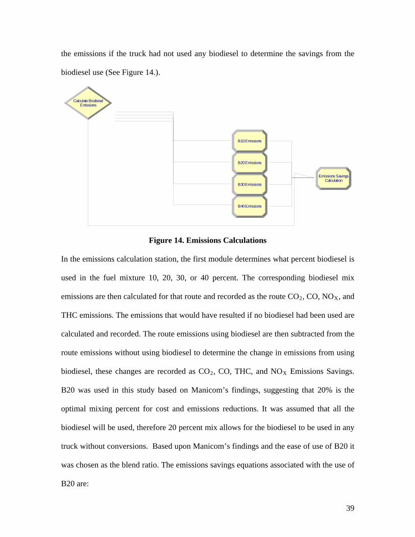
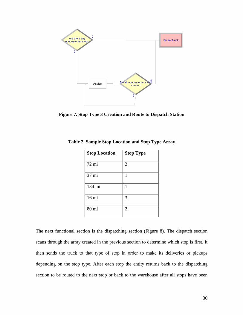
the emissions if the truck had not used any biodiesel to determine the savings from the
biodiesel use (See Figure 14.).
EmissionsCalculate Biodiesel
B40 Emissions
B30 Emissions
B20 Emissions
B10 Emissions
CalculationEmissions Savings
Figure 14. Emissions Calculations In the emissions calculation station, the first module determines what percent biodiesel is
used in the fuel mixture 10, 20, 30, or 40 percent. The corresponding biodiesel mix
emissions are then calculated for that route and recorded as the route CO2, CO, NOX, and
THC emissions. The emissions that would have resulted if no biodiesel had been used are
calculated and recorded. The route emissions using biodiesel are then subtracted from the
route emissions without using biodiesel to determine the change in emissions from using
biodiesel, these changes are recorded as CO2, CO, THC, and NOX Emissions Savings.
B20 was used in this study based on Manicom’s findings, suggesting that 20% is the
optimal mixing percent for cost and emissions reductions. It was assumed that all the
biodiesel will be used, therefore 20 percent mix allows for the biodiesel to be used in any
truck without conversions. Based upon Manicom’s findings and the ease of use of B20 it
was chosen as the blend ratio. The emissions savings equations associated with the use of
B20 are:
39

Equation Set 2. Emissions Calculations
−⎟⎟⎠
⎞⎜⎜⎝
⎛×××= 22 20 COtCoefficienEmissionsBHPTruck
SpeedAvgMPGCollectedWCOSavingsCO
⎟⎟⎠
⎞⎜⎜⎝
⎛×× 2
tanCOtCoefficienEmissionsDieselHPTruck
SpeedAvgTraveledceDis
−⎟⎟⎠
⎞⎜⎜⎝
⎛×××= COtCoefficienEmissionsBHPTruck
SpeedAvgMPGCollectedWCOSavingsCO 20
⎟⎟⎠
⎞⎜⎜⎝
⎛×× COtCoefficienEmissionsDieselHPTruck
SpeedAvgTraveledceDis tan
−⎟⎟⎠
⎞⎜⎜⎝
⎛×××= THCtCoefficienEmissionsBHPTruck
SpeedAvgMPGCollectedWCOSavingsTHC 20
⎟⎟⎠
⎞⎜⎜⎝
⎛×× THCtCoefficienEmissionsDieselHPTruck
SpeedAvgTraveledceDis tan
−⎟⎟⎠
⎞⎜⎜⎝
⎛×××= NOXX tCoefficienEmissionsBHPTruck
SpeedAvgMPGCollectedWCOSavingsNO 20
⎟⎟⎠
⎞⎜⎜⎝
⎛×× NOXtCoefficienEmissionsDieselHPTruck
SpeedAvgTraveledceDis tan
With the route complete and cost and emissions savings calculated, the reporting section
provides a way to easily view the outputs of the model. The outputs that are reported are,
total cost, biodiesel cost savings, total cost after biodiesel savings, quantity of WCO
collected, CO2, CO, NOX, and THC Savings, the number of trucks that could be fueled at
the specified percentage using the biodiesel from this trucks routes, the amount of
biodiesel produced, and the cost of collecting WCO and producing biodiesel (See Figure
15.). Once all these outputs are reported, the truck waits for the next morning when it can
be routed to the routes setup station. This repeats until the number of specified routes
have all been made.
40

routeWait for next
Cost Savings WCO Collection CO EmissionsCost after Savings
To Route reset
THC CO2
NOX Trucks fueled loop costTotal biodieselbio
Figure 15. Reporting Section
4.3 Verification and Validation The model was constructed based on information from a real system. The model was also
evaluated by other programmers who were familiar with the system and the Arena 7.01
software to verify that the model was constructed in a logical manner. The model was
also run under different inputs to determine proper output control. For example, the
density of stop types was checked to make sure that the inputted number of each stop was
occurring in the model. The cost of fuel parameters were changed to see if the total cost
was affected accordingly. Also the times associated with stopping were manipulated to
see how the route times and cost changed. The outcomes of these tests show that the
model was created to respond similarly to the real system.
The model was built to accommodate real values to be entered from companies. By
allowing for real data to be inputted, the model can provide the information needed by the
company to make decisions regarding this system. This insures that the results are
aligned with the system being modeled.
41

4.4 Experimental Design A series of experiments were conducted to analyze the trends in cost and CO2 savings,
under different parameters for both the full and hybrid piggy back scenarios. The
experimentation takes place over 20 days of routes for all analysis cases. CO2 was chosen
as the indicator for emissions reductions due to the interest in reducing GHG emissions.
Also, the responses in total hydrocarbon and carbon monoxide emissions will follow the
same patterns as CO2. On the other hand, NOX emissions will increase from biodiesel
use. The cause of the opposite trend for NOX can be attributed to the increase of NOX
emissions for biodiesel compared to regular diesel. All the other emissions are reduced
when using biodiesel.
The model will be used to answer the following questions:
1. Is the operation of recovering and trading WCO for biodiesel economically
feasible under the full piggy back decentralized scenario? Why or why not?
a) What are the savings that can be achieved?
2. Is the operation of recovering and trading WCO for biodiesel economically
feasible under the hybrid piggy back decentralized scenario? Why or why not?
a) What are the savings that can be achieved?
3. Is the environmental impact of recovering and trading WCO for biodiesel reduced
under the full piggy back decentralized scenario, compared to the current system? Why or
Why not?
a) What are the emissions reductions that can be achieved?
42

4. Is the environmental impact of recovering and trading WCO for biodiesel reduced
under the hybrid piggy back decentralized scenario, compared to the current system?
Why or Why not?
a) What are the emissions reductions that can be achieved?
5. Is the full or hybrid piggy back scenario more beneficial in terms of economics
and the environment? Under what conditions?
a) What are the differences?
b) What factors have the biggest influence on the outcome of the model?
c) What are the effects to service level caused by the extra time and distance
associated with the collection of WCO?
With these questions answered it will be possible for the F&B industry to determine
which companies have the right fit to utilize the WCO from their customers or for each
distributor to analyze its own situation. This study will also provide insight into areas for
improvement, as well as provide other distribution sectors the understanding of the
potential for closing material loops as it may pertain to their industry.
The factors that were manipulated in the experiment for the full piggy system were the
cost of diesel, cost of biodiesel, time at each stop, number of stops with WCO compared
to the number without WCO (stop type density), total distance traveled, the percentage of
the truck that is filled with products at route start (packing percent), the amount of WCO
picked up at each WCO producing stop (WCO collected), and the volume of products
delivered at each customer stop (See Table 3). These factors values were all changed by
25% in both the positive and negative directions from baseline to be used in the fractional
factorial design. The eight factors were used to build a 28-3 fractional factorial design to
43

test which factors have a significant impact on the systems cost and CO2 emissions. This
same strategy was applied to the hybrid piggy back system, however the hybrid method
included 2 more factors, additional non-customer stops and the maximum addition
distance traveled for each additional non-customer stop (See Table 3). The experimental
design used to analyze this system was a 210-5. Both experiments had 32 treatment
combinations. The full system was a 1/8 fraction of the full factorial design while the
hybrid system was a 1/32 fraction of the full factorial design. Because the experiments
were not full factorials, some effects were aliased. This experiment is a screening
iteration to condense the experiment further in order to provide less aliased results in the
subsequent experiments. The second iteration of experiments for the full piggy back
system will be a 26-1 fractional factorial, see table 9, and the hybrid piggy back system
will be a 28-3 fractional factorial. A full factorial experiment was not conducted based on
time constraints. The full and hybrid experimental designs are shown in tables 5 and 6
respectively.
44

Table 3. Factors and Their Corresponding Baseline Values for the Full and Hybrid Piggy Back Scenarios
Factors Full System Baseline Values Hybrid System Baseline Values
Diesel Cost $3.00 $3.00
Biodiesel Cost $1.00 $1.00
Stop Time 10 mins 10 mins
Stop Density 10 Without WCO, 5 With 10 Without WCO, 5 With
Total Distance 22 + 275 * BETA(0.896, 2.77) 22 + 275 * BETA(0.896, 2.77)
Packing % TRIA(0.3, 0.951, 1) TRIA(0.3, 0.951, 1)
WCO Collected UNIF(16,23) UNIF(16,23)
Product Volume TRIA(1.26e+4, 1.8e+4, 8.93e+4) TRIA(1.26e+4, 1.8e+4, 8.93e+4)
Non-customers N/A 4 Additional Stops
Add Distance N/A 10 mi
Table 4. Experimental Design Factors
A = Diesel Cost B = Biodiesel Cost C =Delay time D = Stop Density E = Distance F = Packing percent G = WCO H = Product volume I = Non customer J = Additional Distance
45

Table 5. Aliasing Structure for 28-3 Fractional Factorial Design
Design GeneratorsF = ABC G = ABD H = BCDE
Defining Relationship: I = ABCF = ABDG = CDFG = BCDEH = ADEFH = ACEGH = BEFGH
AliasesA = BCF = BDG AE = DFH = CGH DE = BCH = AFHB = ACF = ADG AF = BC = DEH DH = BCE = AEFC= ABF = DFG AG = BD = CEH EF = ADH = BGHD = ABG = CFG AH = DEF = CEG EG = ACH = BFHE = BE = CDH = FGH EH = BCD = ADF = ACG = BFGF = ABC = CDG BH = CDE = EFG FH = ADE = BEGG = ABD = CDF CD = FG = BEH GH = ACE = BEFH = CE = BDH = AGH ABE = CEF = DEGAB = CF = DG CG = DF = AEH ABH = CFH = DGHAC = BF = EGH CH = BDE = AEG ACD = BDF = BCG = AFGAD = BG = EFH
Table 6. Aliasing Structure for 210-5 Fractional Factorial Design
Design GeneratorsF = ABCD G = ABCE H = ABDE J = ACDE K = BCDE
Defining Relationship: I = ABCDF = ABCEG = DEFG = ABDEH = CEFH = CDGH = ABFGH = ACDEJ =BEFJ = BDGJ = ACFGJ = BCHJ = ADFHJ = AEGHJ = BCDEFGHJ = BCDEK = AEFK = ADGK = BCFGK = ACHK = BDFHK = BEGHK = ACDEFGHK = ABJK = CDFJK = CEGJK = ABDEFGJK = DEHJK = ABCEFHJK = ABCDGHJK = FGHJK
AliasesA = EFK = DGK = CHK = BJK AH = BDE = BFG = DFJ = EGJ = CK B = EFJ = DGJ = CHJ = AJK AJ = CDE = CFG = DFH = EGH = BKC = EFH = DGH = BHJ = AHK AK = EF = DG = CH = BJD = EFG = CGH = BGJ = AGK BC = ADF = AEG = HJ = DEK = FGK E = DFG = CFH = BFJ = AFK BD = ACF = AEH = GJ = CEK = FHKF = DEG = CEH = BEJ = AEK BE = ACG = ADH = FJ = CDK = GHKG = DEF = CDH = BDJ = ADK BF = ACD = AGH = EJ = CGK = DHKH = CEF = CDG = BCJ = ACK BG = ACE = AFH = DJ = CFK = EHKJ = BEF = BDG = BCH = ABK BH = ADE = AFG = CJ = DFK = EGKK = AEF = ADG = ACH =ABJ CD = ABF = GH = AEJ = BEK = FJKAB = CDF = CEG = DEH = FGH = JK CE = ABG = FH = ADJ = BDK = GJKAC = BDF = BEG = DEJ = FGJ = HK CF = ABE = EH = AGJ = BGK = DJK AD = BCF = BEH = CEJ = FHJ = GK CG = ABE = DH = AFJ = BFK = EJKAE = BCG = BDH = CDJ = GHJ = FK DE = FG = ABH = ACJ = BCK = HJKAF = BCD = BGH = CGJ = DHJ = EK DF = ABC = EG = AHJ = BHK = CJKAG = BCE = BFH = CFJ = EHJ = DK
46

The number of replications for each treatment combination was chosen to be 10,000. This
number was chosen because of the relatively fast run time of the model and its good
estimation of the confidence interval. This large number of replications also provides for
an accurate analysis of the system.
5. Full Piggy Back System Results
When analyzing the results from the full piggy back system under the resolution IV 28-3
design, it can be seen by the ANOVA tables in Tables 7 and 8, that the main effects are
driving cost and CO2 savings under these conditions. While the F statistics for 2-way
interactions for both cost and CO2 are significant, they do not seem practically relevant in
comparison to the main effects when comparing the magnitudes of their F statistics in
tables 7 and 8. The F statistics for the main effects in both responses are at least an order
of magnitude greater than that of the 2-way interactions. The fact that the 2-way
interactions are considered statistically relevant is most likely due to the large number of
replications and that the fractional factorial design is aliasing interactions together. When
looking at the factors and interactions alone, it can further be seen that the main effects
are really driving the cost and CO2 savings in the system under these conditions and
assumptions.
Because the P-values in the estimated effects and coefficients tables for both cost and
CO2 savings show significance for factors that do not seem practically relevant (for
example refer to table 10), the sums of squares (effects) and the response plots are used to
determine how strong the factor or interaction effect is on the given response in the
following results sections.
47
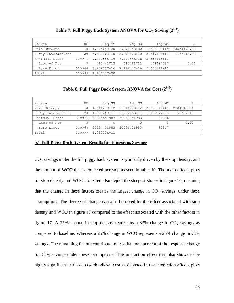
Table 7. Full Piggy Back System ANOVA for CO2 Saving (28-3) Source DF Seq SS Adj SS Adj MS F Main Effects 8 1.37464E+20 1.37464E+20 1.71830E+19 73573470.32 2-Way Interactions 20 5.49826E+18 5.49826E+18 2.74913E+17 1177113.33 Residual Error 319971 7.47288E+16 7.47288E+16 2.33549E+11 Lack of Fit 3 460461712 460461712 153487237 0.00 Pure Error 319968 7.47288E+16 7.47288E+16 2.33551E+11 Total 319999 1.43037E+20
Table 8. Full Piggy Back System ANOVA for Cost (28-3) Source DF Seq SS Adj SS Adj MS F Main Effects 8 1.64427E+12 1.64427E+12 2.05534E+11 2189648.64 2-Way Interactions 20 1.05726E+11 1.05726E+11 5286277223 56317.17 Residual Error 319971 30034451983 30034451983 93866 Lack of Fit 3 0 0 0 0.00 Pure Error 319968 30034451983 30034451983 93867 Total 319999 1.78003E+12
5.1 Full Piggy Back System Results for Emissions Savings
CO2 savings under the full piggy back system is primarily driven by the stop density, and
the amount of WCO that is collected per stop as seen in table 10. The main effects plots
for stop density and WCO collected also depict the steepest slopes in figure 16, meaning
that the change in these factors creates the largest change in CO2 savings, under these
assumptions. The degree of change can also be noted by the effect associated with stop
density and WCO in figure 17 compared to the effect associated with the other factors in
figure 17. A 25% change in stop density represents a 33% change in CO2 savings as
compared to baseline. Whereas a 25% change in WCO represents a 25% change in CO2
savings. The remaining factors contribute to less than one percent of the response change
for CO2 savings under these assumptions The interaction effect that also shows to be
highly significant is diesel cost*biodiesel cost as depicted in the interaction effects plots
48

in Figure 18. The interaction between diesel cost and biodiesel cost should not logically
effect the CO2 emissions in anyway. CO2 savings as dictated by its equation is based
upon, the distances traveled, speed, the horse power of the truck, and the amount of WCO
collected.
CO2 Savings Equation:
−⎟⎟⎠
⎞⎜⎜⎝
⎛×××= 22 20 COtCoefficienEmissionsBHPTruck
SpeedAvgMPGCollectedWCOSavingsCO
⎟⎟⎠
⎞⎜⎜⎝
⎛×× 2
tanCOtCoefficienEmissionsDieselHPTruck
SpeedAvgTraveledceDis
The calculation of CO2 is not effected by the cost of diesel or biodiesel in any way. The
significance of the interaction between diesel cost and biodiesel cost could be explained
using the aliasing structure. With the 28-3 design, diesel cost*biodiesel cost are aliased
with the two most significant factors interaction, WCO collected*stop density plus it is
also aliased with delay time*packing percent as seen in table 5 (AB = CD = FG). The
aliasing structure also confounds the significance of WCO collected*stop density
therefore its significance or relative importance cannot be determined directly. However,
seeing that the effects value for diesel cost*biodiesel cost is so large in table 10, and the
fact that it should have no logical effects on CO2, as noted earlier, suggest that the
interaction of WCO collected and stop density are significant and showing through in the
response plots for diesel cost*biodiesel cost in figure 18. These two interactions are also
aliased with delay time*packing percent which also should have no effect on CO2
savings either, as noticed by the equation for calculating CO2 savings. Looking at the
interaction effects plot for diesel cost*biodiesel cost and delay time*packing percent in
figure 18 aids in validating the theory that the interaction between WCO and stops
49

density is showing through in both the interactions of diesel cost*biodiesel cost and delay
time*packing percent. The two interaction effects are identical yet neither should have
any effect on the CO2 savings, and they are both aliased with WCO*Stop density as
depicted in the interaction effects plots in figure 18. To further understand this
interaction, the design was reduced from a 28-3 to a 26-1 1/2 fraction factorial.
Table 9. Aliasing Structure for 26-1 Fractional Factorial Design
Design GeneratorsI = ACDF
AliasesA = CDF AE = CDEFB = ABCDF AF = CDC = ADF BC = ABCFD = ACF BD = ABCFE = ACDEF BE = ABDEFF = ACD BF = ABCDAB = CDF CE = ADEF AC = DF DE = ACEFAD = CF EF = ACDE
This was done by eliminating the two factors that seem to have minimal effect, or a flat
response line, on CO2 savings. The factors showing the no effect on CO2 savings were
packing percent and product volume (See Figure 16). With these factors removed, the
interaction diesel cost*biodiesel cost is only aliased with WCO collected*stop density.
With the 26-1 design the interaction between diesel cost*biodiesel cost was significant but
not practically relevant, this further supports the fact that WCO collected*stop density is
the interaction that is showing through to be significant. The pareto chart in seen in
Figure 18 shows the impacts to the responses by the individual factor and the interaction.
The pareto chart shows no practical relevance for the interaction between diesel cost and
biodiesel cost. No other interaction effects seem to have any practical relevance to the
50

CO2 savings response as shown in the pareto chart and interaction plots for CO2 savings
under the full piggy back system in figures 17 and 18 respectively.
Table 10. Estimates Effects and Coefficients for CO2 Savings (28-3) Estimated Effects and Coefficients for CO2 Savings (coded units) Term Effect Coef SE Coef T P Constant 49745169 854.3 58228.72 0.000 diesel cost -0 -0 854.3 -0.00 1.000 biodiesel cost 0 0 854.3 0.00 1.000 Delay time -0 -0 854.3 -0.00 1.000 Stop Density 33161013 16580506 854.3 19408.15 0.000 Distance 910 455 854.3 0.53 0.595 Packing percent 0 0 854.3 0.00 1.000 WCO 24872584 12436292 854.3 14557.18 0.000 Product volume 0 0 854.3 0.00 1.000 diesel cost*biodiesel cost 8290253 4145127 854.3 4852.04 0.000 diesel cost*Delay time 0 0 854.3 0.00 1.000 diesel cost*Stop Density 0 0 854.3 0.00 1.000 diesel cost*Distance 0 0 854.3 0.00 1.000 diesel cost*Packing percent 0 0 854.3 0.00 1.000 diesel cost*WCO -0 -0 854.3 -0.00 1.000 diesel cost*Product volume -0 -0 854.3 -0.00 1.000 biodiesel cost*Distance 0 0 854.3 0.00 1.000 biodiesel cost*Product volume 0 0 854.3 0.00 1.000 Delay time*Stop Density -0 -0 854.3 -0.00 1.000 Delay time*Distance -0 -0 854.3 -0.00 1.000 Delay time*WCO -0 -0 854.3 -0.00 1.000 Delay time*Product volume 0 0 854.3 0.00 1.000 Stop Density*Distance 303 152 854.3 0.18 0.859 Stop Density*Product volume -0 -0 854.3 -0.00 1.000 Distance*Packing percent 0 0 854.3 0.00 1.000 Distance*WCO 227 114 854.3 0.13 0.894 Distance*Product volume 0 0 854.3 0.00 1.000 Packing percent*Product volume 0 0 854.3 0.00 1.000 WCO*Product volume -0 -0 854.3 -0.00 1.000 S = 483269 R-Sq = 99.95% R-Sq(adj) = 99.95%
51

Mea
n of
CO
2
10
60000000
50000000
40000000
10 10
10
60000000
50000000
40000000
10 10
10
60000000
50000000
40000000
10
diesel cost biodiesel cost Delay time
Stop Density Distance Packing percent
WC O Product v olume
Main Effects Plot (data means) for CO2 Savings
Figure 16. Main effects plot for CO2 Savings (28-3)
Mean CO2 Savings
0 5000000 10000000 15000000 20000000 25000000 30000000 35000000
Diesel Cost
Biodiesel Cost
Delay Time
Packing Percent
Product Volume
Distance
WCO
Stop Density
Effect
Figure 17. Pareto of Main Effects Response Values for CO2 Savings
52
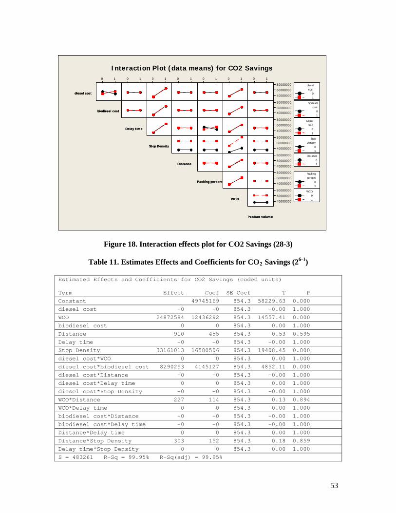
diesel costdiesel cost
Delay timeDelay time
Stop DensityStop Density
DistanceDistance
Packing percentPacking percent
WCOWCO
Product volumeProduct volume
biodiesel costbiodiesel cost
10 10 10 10 10 10 10
80000000
60000000
40000000
80000000
60000000
40000000
80000000
60000000
40000000
80000000
60000000
40000000
80000000
60000000
40000000
80000000
60000000
40000000
80000000
60000000
40000000
dieselcost
01
biodieselcost
01
Delaytime
01
StopDensity
01
Distance01
Packingpercent
01
WCO01
Interaction Plot (data means) for CO2 Savings
Figure 18. Interaction effects plot for CO2 Savings (28-3)
Table 11. Estimates Effects and Coefficients for CO2 Savings (26-1) Estimated Effects and Coefficients for CO2 Savings (coded units) Term Effect Coef SE Coef T P Constant 49745169 854.3 58229.63 0.000 diesel cost -0 -0 854.3 -0.00 1.000 WCO 24872584 12436292 854.3 14557.41 0.000 biodiesel cost 0 0 854.3 0.00 1.000 Distance 910 455 854.3 0.53 0.595 Delay time -0 -0 854.3 -0.00 1.000 Stop Density 33161013 16580506 854.3 19408.45 0.000 diesel cost*WCO 0 0 854.3 0.00 1.000 diesel cost*biodiesel cost 8290253 4145127 854.3 4852.11 0.000 diesel cost*Distance -0 -0 854.3 -0.00 1.000 diesel cost*Delay time 0 0 854.3 0.00 1.000 diesel cost*Stop Density -0 -0 854.3 -0.00 1.000 WCO*Distance 227 114 854.3 0.13 0.894 WCO*Delay time 0 0 854.3 0.00 1.000 biodiesel cost*Distance -0 -0 854.3 -0.00 1.000 biodiesel cost*Delay time -0 -0 854.3 -0.00 1.000 Distance*Delay time 0 0 854.3 0.00 1.000 Distance*Stop Density 303 152 854.3 0.18 0.859 Delay time*Stop Density 0 0 854.3 0.00 1.000 S = 483261 R-Sq = 99.95% R-Sq(adj) = 99.95%
53

Term
Standardized Effect
BDF
DBDBCAFCDAB
FDEADCFACCE
CAE
AE
20000150001000050000
2F actor
Delay timeE S top DensityF diesel cost
NameA WC OB biodiesel costC D istanceD
Pareto Chart of the Standardized Effects(response is CO2 Savings, Alpha = .05)
Figure 19. Pareto Chart of the Standardized effects for CO2 savings
Mea
n of
CO
2
10
70000000
60000000
50000000
40000000
3000000010 10
10
70000000
60000000
50000000
40000000
3000000010 10
WCO biodiesel cost Distance
Delay time Stop Density diesel cost
Main Effects Plot (data means) for CO2 Savings
Figure 20. Main effects plot for CO2 Savings (26-1)
54

WCOWCO
DistanceDistance
Delay timeDelay time
Stop DensityStop Density
diesel costdiesel cost
biodiesel costbiodiesel cost
10 10 10 10 10
80000000
60000000
40000000
80000000
60000000
40000000
80000000
60000000
40000000
80000000
60000000
40000000
80000000
60000000
40000000
WCO01
biodieselcost
01
Distance01
Delaytime
01
StopDensity
01
Interaction Plot (data means) for CO2 Savings
Figure 21. Interaction effects plot for CO2 Savings (26-1)
Stop density was investigated more thoroughly because this factor had the larger effect
on CO2 savings under these assumptions. All possible stop densities up to 15 stops, under
the baseline values as reported in Table 3, were examined to understand what degree of
CO2, CO, THC, and NOX emissions savings could be achieved under the full piggy back
system with this configuration figures 22 - 24.
55

CO2 Savings Vs Number of Stops Generating WCO
R2 = 0.9974
-20000000
0
20000000
40000000
60000000
80000000
100000000
120000000
140000000
1600000000 1 2 3 4 5 6 7 8 9 10 11 12 13 14 15
Number of Stops Generating WCO
CO
Sav
ings
(g)
Figure 22. CO2 Savings Vs Number of Stops Generating WCO out of 15 Total Stops
−⎟⎟⎠
⎞⎜⎜⎝
⎛×××= 22 20 COtCoefficienEmissionsBHPTruck
SpeedAvgMPGCollectedWCOSavingsCO
⎟⎟⎠
⎞⎜⎜⎝
⎛×× 2
tanCOtCoefficienEmissionsDieselHPTruck
SpeedAvgTraveledceDis
56

CO and THC Emissions Savings Vs Number of Stops Generating WCO
R2 = 0.9968
R2 = 0.9972
-50000
0
50000
100000
150000
200000
2500000 1 2 3 4 5 6 7 8 9 10 11 12 13 14 15
Number of Stops Generating WCO
Emis
sion
s S
avin
gs (g
)
COTHC
Figure 23. CO and THC Savings Vs Number of Stops Generating WCO out of 15 Total Stops
−⎟⎟⎠
⎞⎜⎜⎝
⎛×××= COtCoefficienEmissionsBHPTruck
SpeedAvgMPGCollectedWCOSavingsCO 20
⎟⎟⎠
⎞⎜⎜⎝
⎛ D×× COtCoefficienEmissionsDieselHPTruck
SpeedAvgTraveledceis tan
−⎟⎟⎠
⎞⎜⎜⎝
⎛×××= THCtCoefficienEmissionsBHPTruck
SpeedAvgMPGCollectedWCOSavingsTHC 20
⎟⎟⎠
⎞⎜⎜⎝
⎛×× THCtCoefficienEmissionsDieselHPTruck
SpeedAvgTraveledceDis tan
57

NOX Savings Vs Number of Stops Generating WCO
R2 = 0.9811
-200000
-180000
-160000
-140000
-120000
-100000
-80000
-60000
-40000
-20000
00 2 4 6 8 10 12 14 1
Number of Stops Generating WCO
NOX
Sav
ings
(g)
6
Figure 24. NOX Savings Vs Number of Stops Generating WCO out of 15 Total Stops
−⎟⎟⎠
⎞⎜⎜⎝
⎛×××= NOXX tCoefficienEmissionsBHPTruck
SpeedAvgMPGCollectedWCOSavingsNO 20
⎟⎟⎠
⎞⎜⎜⎝
⎛×× NOXtCoefficienEmissionsDieselHPTruck
SpeedAvgTraveledceDis tan
Increasing stop density increases CO2, CO, and THC emissions savings as shown in
figures 22 and 23. The increase in emissions savings for these emissions can be noted by
the increasing slope in figures 22 and 23. Therefore, it can be inferred that WCO should
be collected from as many customers as possible, using the full piggy back system under
these assumptions. NOx savings is reduced with each additional WCO generating stop
due to NOX being emitted at a higher rate from biodiesel than regular diesel as shown by
the downward slope in figure 24. All 0 stop values in figures 22-24 are negative due to
58

the fact that if no biodiesel is collected the emissions savings is zero and the resulting
emissions that diesel emits is reported.
5.2 Full Piggy Back System Results for Cost and Service Level
The cost response to the full piggy back system is also largely controlled by the main
effects as was revealed by comparing the F statistics in the ANOVA table in Table 7
above. The individual factors that have the most prevalent effect in order from, largest to
smallest are stop density, diesel cost, and WCO collected as seen in the effects values in
Table 12 and steep slopes in the effects plots of figure 25. A 25% change in these factors
represents 282%, 280%, and 225% change in cost respectively, compared to the baseline
full piggy back system. The other factors that are helping drive the cost response under
these assumptions are distance, biodiesel cost, and stop time, they represent a 115%,
84%, 71% change in cost respectively compared to the baseline full piggy back system.
The values associated with the change in cost associated with each factor are visually
presents in the pareto diagram in figure 26. When looking at the interaction effects for
cost under the full piggy back system, diesel cost*biodiesel cost, diesel cost*stop density,
diesel cost*WCO, and diesel cost*distance are all significant and practically relevant as
suggested by the large values associated with their effects in table 12. These interactions
follow logical patterns that would be expected from this system, based upon the relevance
of their main effects and that these factors are incorporated into the cost equations.
59

Cost of labor (L) = Time (T)*Wage (W) Cost of Diesel Fuel (CD) = ((0.8 *Distance (D))/Fuel Economy (E))* Price of Diesel (FD) Cost of Additional Labor (LA) = Additional Time (TA)* Wage (W) Cost of Additional Diesel (CDA) = ((0.8 *Additional Distance (DA))/Fuel Economy (E))* Price of Diesel (FD) Total Cost of Route (CT) = L + LA + CD + CDA + CB + CBA Cost Savings from Trading all WCO for Biodiesel (S) = ((Total WCO collected (G) * .9) * Price of Diesel (FD)) - ((Total WCO collected (G) * .9) * Price of Biodiesel (FB)) Total Cost of System after Savings (CS) = (L + LA + ((D/E)* FD) + ((DA/E)*FD)) – S For example, a WCO collection system would be expected to respond significantly to the
amount of WCO collected and the cost of fuel. This is seen in the trend of diesel
cost*stop density. The trend suggests that when diesel cost is high the saving from
biodiesel happens at a greater rate, when collecting WCO from a low density of stops to a
high density, than when diesel cost is low (Figure 27). This makes logical sense because
the savings from the use of biodiesel is based on the difference in fuel costs and the
amount of biodiesel that can be produced from the collected WCO. Therefore, if the cost
of diesel is high and the number of stops with WCO goes from low to high you expect to
see a large decrease in cost. Whereas, if diesel cost is low and the stop density goes from
low to high you see a similar trend but a reduced slope signifying a smaller change in
cost savings.
60
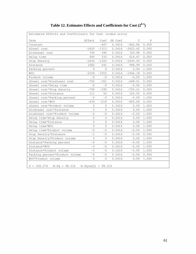
Table 12. Estimates Effects and Coefficients for Cost (28-3) Estimated Effects and Coefficients for Cost (coded units) Term Effect Coef SE Coef T P Constant -467 0.5416 -862.86 0.000 diesel cost -2625 -1313 0.5416 -2423.62 0.000 biodiesel cost 790 395 0.5416 729.08 0.000 Delay time 666 333 0.5416 614.47 0.000 Stop Density -2644 -1322 0.5416 -2440.55 0.000 Distance 1082 541 0.5416 998.99 0.000 Packing percent 0 0 0.5416 0.00 1.000 WCO -2106 -1053 0.5416 -1944.18 0.000 Product volume -0 -0 0.5416 -0.00 1.000 diesel cost*biodiesel cost -702 -351 0.5416 -648.01 0.000 diesel cost*Delay time -0 -0 0.5416 -0.00 1.000 diesel cost*Stop Density -790 -395 0.5416 -729.21 0.000 diesel cost*Distance 111 56 0.5416 102.93 0.000 diesel cost*Packing percent -0 -0 0.5416 -0.00 1.000 diesel cost*WCO -439 -219 0.5416 -405.06 0.000 diesel cost*Product volume 0 0 0.5416 0.00 1.000 biodiesel cost*Distance 0 0 0.5416 0.00 1.000 biodiesel cost*Product volume -0 -0 0.5416 -0.00 1.000 Delay time*Stop Density 0 0 0.5416 0.00 1.000 Delay time*Distance 0 0 0.5416 0.00 1.000 Delay time*WCO 0 0 0.5416 0.00 1.000 Delay time*Product volume -0 -0 0.5416 -0.00 1.000 Stop Density*Distance -1 -0 0.5416 -0.54 0.592 Stop Density*Product volume 0 0 0.5416 0.00 1.000 Distance*Packing percent -0 -0 0.5416 -0.00 1.000 Distance*WCO -0 -0 0.5416 -0.00 1.000 Distance*Product volume -0 -0 0.5416 -0.00 1.000 Packing percent*Product volume -0 -0 0.5416 -0.06 0.956 WCO*Product volume 0 0 0.5416 0.00 1.000 S = 306.376 R-Sq = 98.31% R-Sq(adj) = 98.31%
61

Mea
n of
Cos
t
10
1000
0
-1000
10 10
10
1000
0
-1000
10 10
10
1000
0
-1000
10
diesel cost biodiesel cost Delay time
Stop Density Distance Packing percent
WC O Product v olume
Main Effects Plot (data means) for Cost
Figure 25. Main effects plot for cost (28-3)
Mean Cost
0 500 1000 1500 2000 2500 3000
Product Volume
Delay Time
Biodiesel Cost
Distance
WCO
Diesel Cost
Stop Density
Effect
Figure 26. Pareto of Main Effects Response Values for Cost
62
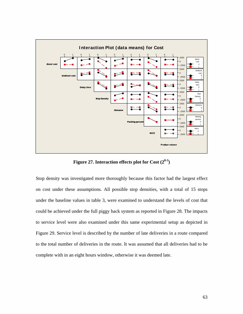
diesel costdiesel cost
Delay timeDelay time
Stop DensityStop Density
DistanceDistance
Packing percentPacking percent
WCOWCO
biodiesel costbiodiesel cost
Product volumeProduct volume
10 10 10 10 10 10 102000
0
-2000
2000
0
-2000
2000
0
-2000
2000
0
-2000
2000
0
-2000
2000
0
-2000
2000
0
-2000
dieselcost
01
biodieselcost
01
Delaytime
01
StopDensity
01
Distance01
Packingpercent
01
WCO01
Interaction Plot (data means) for Cost
Figure 27. Interaction effects plot for Cost (28-3)
Stop density was investigated more thoroughly because this factor had the largest effect
on cost under these assumptions. All possible stop densities, with a total of 15 stops
under the baseline values in table 3, were examined to understand the levels of cost that
could be achieved under the full piggy back system as reported in Figure 28. The impacts
to service level were also examined under this same experimental setup as depicted in
Figure 29. Service level is described by the number of late deliveries in a route compared
to the total number of deliveries in the route. It was assumed that all deliveries had to be
complete with in an eight hours window, otherwise it was deemed late.
63

Cost Vs Number of Stops Generating WCO
R2 = 0.9943
-8000
-6000
-4000
-2000
0
2000
4000
60000 1 2 3 4 5 6 7 8 9 10 11 12 13 14 15
Number fo Stops Generating WCO
Cos
t ($)
Figure 28. Cost Vs Number of Stops Generating WCO out of 15 Total Stops
Service Level Vs Number of Stops Generating WCO
R2 = 0.0252
50
60
70
80
90
100
0 2 4 6 8 10 12 14 16
Number of Stops Generating WCO
Ser
vice
Lev
el (%
)
R2 = 0.9999
Figure 29. Service Level Vs Number of Stops Generating WCO out of 15 Total
Stops
64

Increasing stop density reduces cost as shown by the negative slope in figure 28.
Therefore, it can be inferred that WCO should be collected from as many customers as
possible, using the full piggy back system under these assumptions. The stop density has
no impact to the service level as depicted in figure 28 provided under the full piggy back
system, this further supports the statement that all stops generating WCO should be
collected from under these assumptions. Stop density not effecting service level seems
unintuitive, it would be logical to assume that the added process would impair the ability
to meet customers demand. It is possible that the system that was modeled, was not at full
capacity and or that the assumed additional time for collection of five minute was
underestimeated.
5.3 Effects to the Full Piggy Back System from Changes in Total Number of Stops
The experimentation to this point had been based on the assumption that every route had
15 total customer stops. To determine whether the model outputs would hold true for
different number of total stops, two single factor experiments were conducted with a total
of 10 stops and 30 stops. Within each level of total stops, the stop density was varied
between 20 and 80 percent in increments of 20 percent. The outcome of these
experiments showed that the responses in both cost and CO2 are similar for both 10 stops
and 30 stops at the four levels of stop density (See Figures 30 - 31).
65

Cost and CO2 Savings VS Stop Density for 10 Stops
y = -1319.1x + 2414.2
y = 2E+07x + 8E+06
-3500
-3000
-2500
-2000
-1500
-1000
-500
0
500
1000
1500
Percentage of Stops with WCO
Cost
($)
0
10000000
20000000
30000000
40000000
50000000
60000000
70000000
8000000020 40 60 80
CO2
Savi
ngs
(g)
CostCO2
Figure 30. Response Plot for Cost and CO2 Savings VS Density of Stops with WCO for 10 Total Stops
Cost and CO2 Savings VS Stop Density for 30 Stops
y = 5E+07x + 8E+06
y = -3959.9x + 4078.5
-14000
-12000
-10000
-8000
-6000
-4000
-2000
0
2000
Pecentage of Stops with WCO
Cos
t ($)
0
50000000
100000000
150000000
200000000
25000000020 40 60 80
CO
2 S
avin
gs ($
)
CostCO2
Figure 31. Response Plot for Cost and CO2 Savings VS Density of Stops with WCO for 30 Total Stops
66

When comparing the responses from the different stop densities for 10 and 30 total stops
in figures 30 and 31, it can be seen that they both follow similar trends for cost and CO2
savings. However, when you look at the slope of the line from the equation, it can be seen
that cost decreases and CO2 savings increases at a rate three times more quickly for 30
stops than for 10 stops (Refer to Figures 30 – 31). This is explained by the fact that three
times more stops are visited that generate WCO for a total of 30 stops, and the distance
traveled is the same for both 10 and 30 total stops. The consistency of the results from
these two experiments suggests that the model and conclusions are robust against the
variation of total customer stops.
Total distance does not change based upon the number of stops in the route. The actual
data from the F&B distributor showed no correlation between the number of stops and
the distance traveled for that route as seen in Figure 32.
Number of stops VS Distance Traveled
R2 = 0.0009
0
50
100
150
200
250
300
350
0 10 20 30 40
Number of Stops
Dis
tanc
e Tr
avel
ed (m
i)
Figure 32. Actual Total Distance (Local Distributor) VS Number of Stops
67

6. Hybrid Piggy Back System Results The hybrid piggy back system showed that the main effects were driving the system for
both cost and CO2 savings, under these assumptions. The F statistics for the main effects
for both cost and CO2 savings were at least an order of magnitude larger than the 2-way
interaction effects as seen in tables 13 and 14.
Table 13. Hybrid Piggy Back System ANOVA Table for CO2 Saving (210-5) Source DF Seq SS Adj SS Adj MS F Main Effects 10 2.95927E+20 2.95927E+20 2.95927E+19 6557389.90 2-Way Interactions 21 1.24785E+19 1.24785E+19 5.94214E+17 131670.59 Residual Error 319968 1.44398E+18 1.44398E+18 4.51288E+12 Pure Error 319968 1.44398E+18 1.44398E+18 4.51288E+12 Total 319999 3.09850E+20
Table 14. Hybrid Piggy Back System ANOVA Table for Cost (210-5)
Source DF Seq SS Adj SS Adj MS F Main Effects 10 2.94643E+12 2.94643E+12 2.94643E+11 2488242.69 2-Way Interactions 21 2.70866E+11 2.70866E+11 12898367078 108926.13 Residual Error 319968 37888656223 37888656223 118414 Pure Error 319968 37888656223 37888656223 118414 Total 319999 3.25518E+12
6.1 Hybrid Piggy Back System Emissions Results When analyzing the main and interactions effects on an individual level for CO2 savings
under the hybrid piggy back system, it can be seen that diesel cost, biodiesel cost, delay
time, product volume, and packing percent have little effects, shown as a flat line, on the
response as seen in the effects plots in figure 33 and by the values associated with their
effects in table 15 and figure 34. These factors were selected for removal when analyzing
CO2 savings in order to get a cleaner look at the results. By removing these five factors,
the experiment is reduced to a 25 full factorial. Reducing the experiment to a 25 full
factorial produces no effects that are aliased.
68
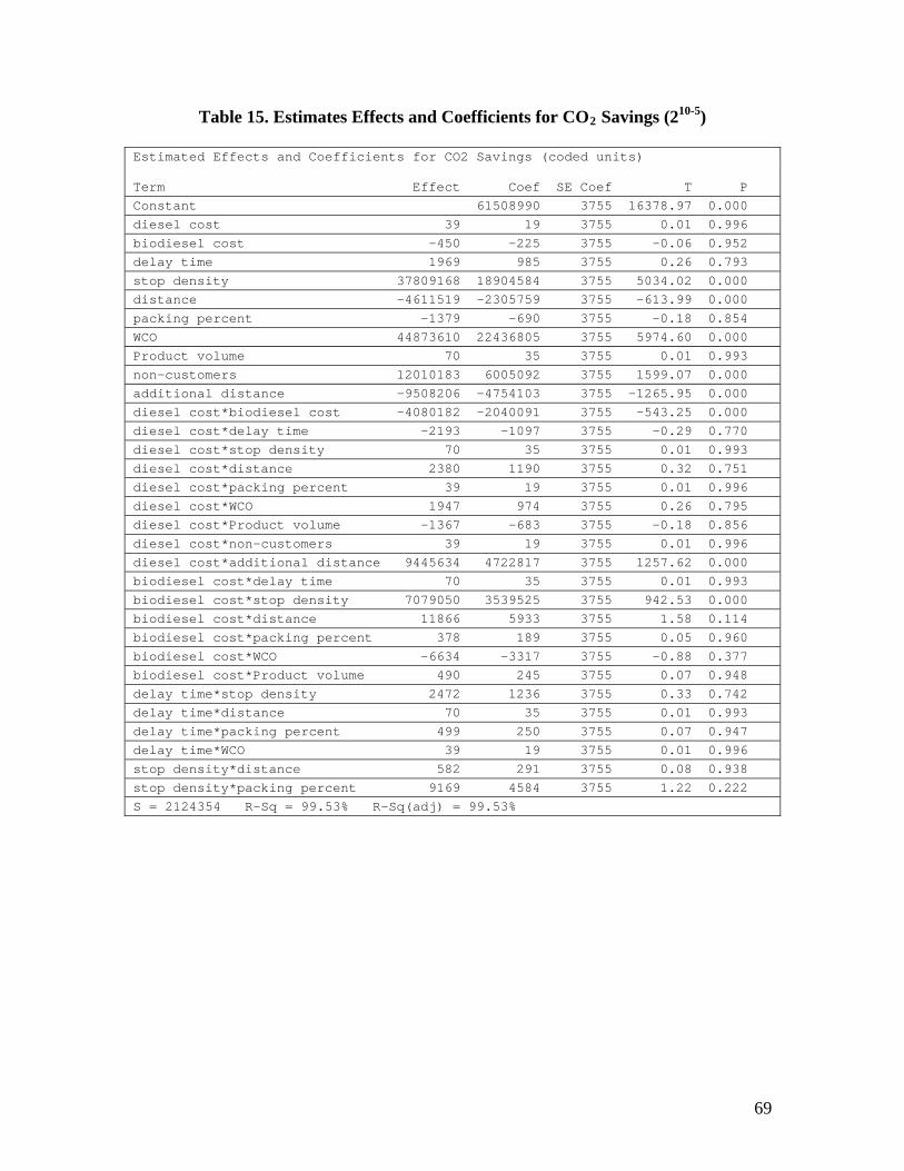
Table 15. Estimates Effects and Coefficients for CO2 Savings (210-5) Estimated Effects and Coefficients for CO2 Savings (coded units) Term Effect Coef SE Coef T P Constant 61508990 3755 16378.97 0.000 diesel cost 39 19 3755 0.01 0.996 biodiesel cost -450 -225 3755 -0.06 0.952 delay time 1969 985 3755 0.26 0.793 stop density 37809168 18904584 3755 5034.02 0.000 distance -4611519 -2305759 3755 -613.99 0.000 packing percent -1379 -690 3755 -0.18 0.854 WCO 44873610 22436805 3755 5974.60 0.000 Product volume 70 35 3755 0.01 0.993 non-customers 12010183 6005092 3755 1599.07 0.000 additional distance -9508206 -4754103 3755 -1265.95 0.000 diesel cost*biodiesel cost -4080182 -2040091 3755 -543.25 0.000 diesel cost*delay time -2193 -1097 3755 -0.29 0.770 diesel cost*stop density 70 35 3755 0.01 0.993 diesel cost*distance 2380 1190 3755 0.32 0.751 diesel cost*packing percent 39 19 3755 0.01 0.996 diesel cost*WCO 1947 974 3755 0.26 0.795 diesel cost*Product volume -1367 -683 3755 -0.18 0.856 diesel cost*non-customers 39 19 3755 0.01 0.996 diesel cost*additional distance 9445634 4722817 3755 1257.62 0.000 biodiesel cost*delay time 70 35 3755 0.01 0.993 biodiesel cost*stop density 7079050 3539525 3755 942.53 0.000 biodiesel cost*distance 11866 5933 3755 1.58 0.114 biodiesel cost*packing percent 378 189 3755 0.05 0.960 biodiesel cost*WCO -6634 -3317 3755 -0.88 0.377 biodiesel cost*Product volume 490 245 3755 0.07 0.948 delay time*stop density 2472 1236 3755 0.33 0.742 delay time*distance 70 35 3755 0.01 0.993 delay time*packing percent 499 250 3755 0.07 0.947 delay time*WCO 39 19 3755 0.01 0.996 stop density*distance 582 291 3755 0.08 0.938 stop density*packing percent 9169 4584 3755 1.22 0.222 S = 2124354 R-Sq = 99.53% R-Sq(adj) = 99.53%
69

Mea
n of
CO
2 Sa
ving
s
10
80000000
60000000
40000000
10 10 10
10
80000000
60000000
40000000
10 10 10
10
80000000
60000000
40000000
10
diesel cost biodiesel cost delay time stop density
distance packing percent WC O Product v olume
noncustomers additional distance
Main Effects Plot (data means) for CO2 Savings
Figure 33. Main Effects plots for CO2 Savings (210-5)
70

Mean CO2 Savings
0 5E+06 1E+07 2E+07 2E+07 3E+07 3E+07 4E+07 4E+07 5E+07 5E+07
Product Volume
Delay Time
Biodiesel Cost
Diesel Cost
Distance
Additional Distance
Non Customers
Stop Density
WCO
Effect
Figure 34. Pareto of Main Effects Response Values for CO2 Savings
With the factorial reduced to a 25 design for CO2 savings, the effects become clearer and
easily analyzed. The ANOVA table for the reduced hybrid design still reports the main
effects as driving the system as revealed by the relatively large F statistic reported for
main effects as compared to interactions in table 16. When looking into the individual
factors, all of them emerge as significant and relevant through the large values associated
with there effects on CO2 savings (Table 17). The main effects response plot confirms
the relevance of the factors on CO2 savings, these factors follow the logical patterns
associated with this system under these assumptions in that all the factors have impacts to
the amount of WCO collected or the distance traveled, which are driving the CO2 savings
equation. (Figure 35). The interaction effects associated with CO2 savings also fit
logically with how the system should work in that if the factor reduces the amount of
71

WCO collected or increases the distance the CO2 savings is reduced and vice versa
(Figure 37). For example, when stop density of customers generating WCO is high and
the amount of WCO collected from each stops increases, CO2 savings increase at a rate
faster than when the stop density is low as seen in the effects plots in Figure 37. These
logical findings help aid in verifying the logic of the model is correct.
Table 16. Hybrid Piggy Back System ANOVA for CO2 Saving (25)
Source DF Seq SS Adj SS Adj MS F Main Effects 5 2.95927E+20 2.95927E+20 5.91855E+19 13115315.14 2-Way Interactions 10 1.24785E+19 1.24785E+19 1.24785E+18 276519.25 Residual Error 319984 1.44399E+18 1.44399E+18 4.51270E+12 Lack of Fit 16 1.32592E+13 1.32592E+13 8.28702E+11 0.18 Pure Error 319968 1.44398E+18 1.44398E+18 4.51288E+12 Total 319999 3.09850E+20
Table 17. Estimates Effects and Coefficients for CO2 Savings (25) Estimated Effects and Coefficients for CO2 Savings (coded units) Term Effect Coef SE Coef T P Constant 61508990 3755 16379.31 0.000 stop density 37809168 18904584 3755 5034.13 0.000 distance -4611519 -2305759 3755 -614.00 0.000 WCO 44873610 22436805 3755 5974.72 0.000 non-customers 12010183 6005092 3755 1599.10 0.000 additional distance -9508206 -4754103 3755 -1265.98 0.000 stop density*distance 582 291 3755 0.08 0.938 stop density*WCO 9445634 4722817 3755 1257.64 0.000 stop density*non-customers -6634 -3317 3755 -0.88 0.377 stop density*additional distance 1947 974 3755 0.26 0.795 distance*WCO 9169 4584 3755 1.22 0.222 distance*non-customers 378 189 3755 0.05 0.960 distance*additional distance 39 19 3755 0.01 0.996 WCO*non-customers 7079050 3539525 3755 942.54 0.000 WCO*additional distance 70 35 3755 0.01 0.993 non-customers*additional distance -4080182 -2040091 3755 -543.26 0.000 S = 2124311 R-Sq = 99.53% R-Sq(adj) = 99.53%
72

Term
S t a nda rd ize d Effe c t
B E
C E
B D
A B
A E
A D
B C
D E
B
C D
A C
E
D
A
C
6000500040003000200010000
2F a cto r
no ncusto m e rsE a dd it io na l d is ta nce
N a m eA sto p de ns ityB d ista nceC W C OD
P a r e to C ha r t o f the S ta nda r dize d E ffe c ts(re sponse is C O 2 S a vings , A lpha = .05)
Figure 35. Pareto Chart of the Standardized Effects for CO2 Savings (25)
Mea
n of
CO
2 Sa
ving
s
10
80000000
70000000
60000000
50000000
40000000
10 10
10
80000000
70000000
60000000
50000000
40000000
10
sto p density d istan ce W C O
no ncusto mers add itio nal d istan ce
Main Effects Plot (data means) for CO 2 S avings
Figure 36. Main Effects plots for CO2 Savings (25)
Each main effect has physical meaning. As stop density increases the amount of WCO
that is collect increases. The larger amounts of collected WCO become increased
amounts of biodiesel that can be used in place of petroleum based diesel, therefore
73

reducing CO2 emissions. The total distance traveled impacts CO2 in that as larger
distances are traveled more CO2 is emitted through the combustion of fuel. Similar to
stop density, as the volume of collected WCO is increased the more biodiesel and
subsequent emissions reduction increase. The same is true for high number of
noncustomers providing WCO. The increase in locations providing WCO, the more
biodiesel and emissions reductions can be realized. The additional distances traveled
however reduces the CO2 saving, based on emissions generated to collect the WCO.
stop densitystop density
WCOWCO
noncustomersnoncustomers
additional distanceadditional distance
distancedistance
10 10 10 10
90000000
60000000
30000000
90000000
60000000
30000000
90000000
60000000
30000000
90000000
60000000
30000000
stopdensity
01
distance01
WCO01
noncustomers01
Interaction Plot (data means) for CO2 Savings
Figure 37. Interaction Effects plots for CO2 Savings (25)
6.2 Hybrid Piggy Back System Results for Cost
This same experimental reduction method that was conducted for reducing the
experiment for CO2 was done for cost. The main effects plots show no change or a flat
response in the cost response from packing percent or product volume, so they were
74
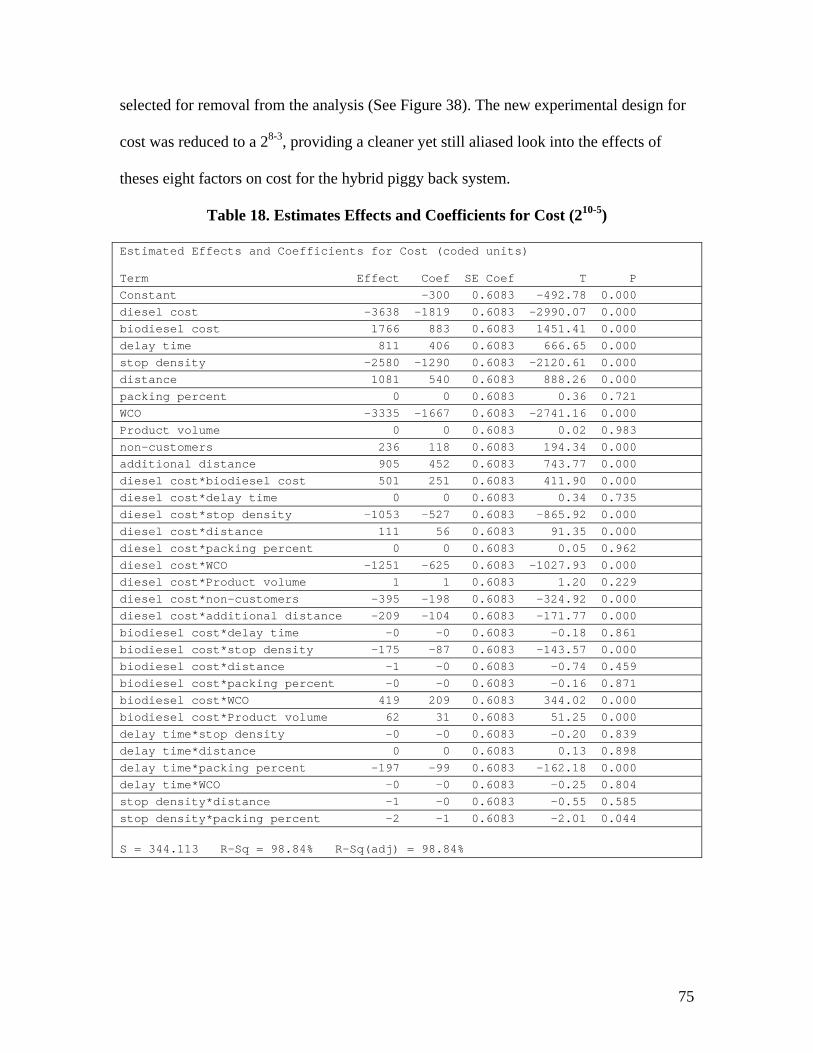
selected for removal from the analysis (See Figure 38). The new experimental design for
cost was reduced to a 28-3, providing a cleaner yet still aliased look into the effects of
theses eight factors on cost for the hybrid piggy back system.
Table 18. Estimates Effects and Coefficients for Cost (210-5) Estimated Effects and Coefficients for Cost (coded units) Term Effect Coef SE Coef T P Constant -300 0.6083 -492.78 0.000 diesel cost -3638 -1819 0.6083 -2990.07 0.000 biodiesel cost 1766 883 0.6083 1451.41 0.000 delay time 811 406 0.6083 666.65 0.000 stop density -2580 -1290 0.6083 -2120.61 0.000 distance 1081 540 0.6083 888.26 0.000 packing percent 0 0 0.6083 0.36 0.721 WCO -3335 -1667 0.6083 -2741.16 0.000 Product volume 0 0 0.6083 0.02 0.983 non-customers 236 118 0.6083 194.34 0.000 additional distance 905 452 0.6083 743.77 0.000 diesel cost*biodiesel cost 501 251 0.6083 411.90 0.000 diesel cost*delay time 0 0 0.6083 0.34 0.735 diesel cost*stop density -1053 -527 0.6083 -865.92 0.000 diesel cost*distance 111 56 0.6083 91.35 0.000 diesel cost*packing percent 0 0 0.6083 0.05 0.962 diesel cost*WCO -1251 -625 0.6083 -1027.93 0.000 diesel cost*Product volume 1 1 0.6083 1.20 0.229 diesel cost*non-customers -395 -198 0.6083 -324.92 0.000 diesel cost*additional distance -209 -104 0.6083 -171.77 0.000 biodiesel cost*delay time -0 -0 0.6083 -0.18 0.861 biodiesel cost*stop density -175 -87 0.6083 -143.57 0.000 biodiesel cost*distance -1 -0 0.6083 -0.74 0.459 biodiesel cost*packing percent -0 -0 0.6083 -0.16 0.871 biodiesel cost*WCO 419 209 0.6083 344.02 0.000 biodiesel cost*Product volume 62 31 0.6083 51.25 0.000 delay time*stop density -0 -0 0.6083 -0.20 0.839 delay time*distance 0 0 0.6083 0.13 0.898 delay time*packing percent -197 -99 0.6083 -162.18 0.000 delay time*WCO -0 -0 0.6083 -0.25 0.804 stop density*distance -1 -0 0.6083 -0.55 0.585 stop density*packing percent -2 -1 0.6083 -2.01 0.044 S = 344.113 R-Sq = 98.84% R-Sq(adj) = 98.84%
75

Mea
n of
Cos
t
10
2000
0
-2000
10 10 10
diesel cost biodiesel cost delay time
10
2000
0
-2000
10 10 10
10
2000
0
-2000
10
stop density
distance packing percent WC O Product v olume
noncustomers additional distance
Main Effects Plot (data means) for Cost
Figure 38. Main Effects plots for Cost (210-5)
The 28-3 design for cost shows a less aliased set of responses than the resolution IV 210-5
design; however it is still aliased under the structure provided in table 5. The results of
the 28-3 still suggest that the main effects for cost are driving the system. This can be
confirmed when looking at the scale of the main effects as compared to the interactions in
the pareto and main effects plots in Figures 39 and 40 respectively. All the responses for
cost under the hybrid piggy back scenario seem to follow how the system would perform
logically, except one. The cost response for the hybrid piggy back system was thought to
be based upon the cost of fuel, time, distance, and the amount of WCO collected. This
can be seen in the main effects plots in figure 40. An increase in the difference in cost
between diesel and biodiesel, diesel cost increasing while biodiesel cost is decreasing,
and an increase in the amount of WCO collected, there should be a decrease in cost.
76

Whereas with a decrease in distance and time it was expected that cost would decrease
with them. These responses are reflected in the main effects plots in figure 40. One of the
factors effects on the cost responses seems counterintuitive. Logically it would seem that
with each additional non-customer stop (non-customers), the cost would decrease. This
decrease would stem from the additional savings associated with the additional WCO that
is collected from the non-customers and used as biodiesel. However, this is not the case.
The response plot for non-customers shows a direct correlation between cost and non-
customer stops as seen by the increasing slope in the plot in figure 40. This increasing
trend shows through in all the interaction effects associated with non-customer stops as
well (See interaction effects plots in Figure 41). The other interaction effects associated
with cost seem to follow logical patterns suggested above, under these assumptions. For
example, when stop density is high and the route distance moves from low to high, cost
increases at the same rate as when stop density is low, however cost is less with a high
level of stop density.
Table 19. Hybrid Piggy Back System ANOVA Table for Cost (28-3) Source DF Seq SS Adj SS Adj MS F Main Effects 8 2.94642E+12 2.94642E+12 3.68303E+11 2874060.47 2-Way Interactions 20 2.67751E+11 2.67751E+11 13387547813 104469.99 Residual Error 319971 41003423721 41003423721 128147 Lack of Fit 3 3114767498 3114767498 1038255833 8768.02 Pure Error 319968 37888656223 37888656223 118414 Total 319999 3.25518E+12
77

Table 20. Hybrid Piggy Back System Estimated Effects and Coefficients for Cost (28-3) Estimated Effects and Coefficients for Cost (coded units) Term Effect Coef SE Coef T P Constant -300 0.6328 -473.70 0.000 diesel cost -3638 -1819 0.6328 -2874.27 0.000 biodiesel cost 1766 883 0.6328 1395.20 0.000 delay time 811 406 0.6328 640.83 0.000 stop density -2580 -1290 0.6328 -2038.48 0.000 distance 1081 540 0.6328 853.86 0.000 WCO -3335 -1667 0.6328 -2635.00 0.000 Non-customers 236 118 0.6328 186.81 0.000 additional distance 905 452 0.6328 714.97 0.000 diesel cost*biodiesel cost 501 251 0.6328 395.95 0.000 diesel cost*delay time 0 0 0.6328 0.33 0.745 diesel cost*stop density -1053 -527 0.6328 -832.38 0.000 diesel cost*distance 111 56 0.6328 87.82 0.000 diesel cost*WCO -1251 -625 0.6328 -988.12 0.000 diesel cost*non-customers -395 -198 0.6328 -312.34 0.000 diesel cost*additional distance -209 -104 0.6328 -165.12 0.000 biodiesel cost*delay time -0 -0 0.6328 -0.17 0.866 biodiesel cost*stop density -175 -87 0.6328 -138.01 0.000 biodiesel cost*distance -1 -0 0.6328 -0.71 0.476 biodiesel cost*WCO 419 209 0.6328 330.70 0.000 delay time*stop density -0 -0 0.6328 -0.19 0.845 delay time*distance 0 0 0.6328 0.12 0.902 delay time*WCO -0 -0 0.6328 -0.24 0.811 delay time*non-customers 62 31 0.6328 49.27 0.000 delay time*additional distance 1 1 0.6328 1.16 0.248 stop density*distance -1 -0 0.6328 -0.52 0.600 distance*WCO -2 -1 0.6328 -1.93 0.053 distance*non-customers -0 -0 0.6328 -0.16 0.876 distance*additional distance 0 0 0.6328 0.05 0.963 S = 357.977 R-Sq = 98.74% R-Sq(adj) = 98.74%
78

Term
Standardized Effect
EHCEEGBCCDCFACDEBECHEFCGAEBDAH
GAGBFABCH
ADE
AFBDFA
300025002000150010005000
2Factor
stop densityE distanceF WC OG noncustomersH additional distance
NameA diesel costB biodiesel costC delay timeD
Pareto Chart of the Standardized Effects(response is Cost, Alpha = .05)
Figure 39. Pareto Chart of the Standardized Effects for Cost (28-3)
Mea
n of
Cos
t
10
2000
0
-2000
10 10
10
2000
0
-2000
10 10
10
2000
0
-2000
10
diesel cost biodiesel cost delay time
stop density distance WC O
noncustomers additional distance
Main Effects Plot (data means) for Cost
Figure 40. Hybrid Piggy Back System Main Effects Plots for Cost (28-3)
79

diesel costdiesel cost
delay timedelay time
stop densitystop density
distancedistance
WCOWCO
noncustomersnoncustomers
additional distanceadditional distance
biodiesel costbiodiesel cost
10 10 10 10 10 10 103000
0
-30003000
0
-30003000
0
-30003000
0
-30003000
0
-30003000
0
-30003000
0
-3000
dieselcost
01
biodieselcost
01
delaytime
01
stopdensity
01
distance01
WCO01
noncustomers01
Interaction Plot (data means) for Cost
Figure 41. Hybrid Piggy Back System Interaction Effects plots for Cost (28-3) The non-customers effect requires further investigation to determine the cause of the
direct correlation to cost. It was thought that the increase in cost could be attributed to the
distance being traveled and extra time necessary to collect the WCO from the non-
customers. In other words the cost associated with driving to the additional stops and the
time to pick up the WCO was larger than the saving achieved from using the WCO as
biodiesel. In order to investigate the effects of additional non-customer stops to the
model, experiments were conducted that placed the additional non-customer stops at
locations requiring a maximum additional distance from 1 to 20 miles off the route, in
increments of 1 mile. The actual distance from the route is based upon the uniform
distribution, allowing for equal likelihood that the stop be anywhere from 0 to the max
distance away from the route deviation point (UNIF(0, Max deviation distance)). The
80

uniform distribution was chosen because it would not be likely for only stops at the max
distance to be visited. It was assumed that the closest stops would be chosen before stops
at a farther distance from the route. Within these setups, four levels of non-customer
stops were added to the route. The four levels were set at 2, 4, 6, and 8 additional non-
customer stops. This setup was used to determine the distance from the route that was too
far, based on cost, to travel for collecting the WCO from non-customer under this design.
The results of this experiment are visually depicted in Figure 42. Looking at the 3-D
response surface for cost, it can be seen that below the threshold of 9 miles roundtrip on
the distance axis, the cost decreases as the number of additional stops increase. Whereas,
above the 9 mile threshold, or the inflection point, the cost increases as the number of
additional stops increase. This reversal in trends can be attributed to the cost associated
with the extra travel distance and time associated with additional non-customer stops. At
and below a maximum deviation distance of 9 miles per stop, the cost savings from using
WCO as biodiesel outweighs the cost incurred by labor and fuel to travel the additional
distance. Whereas, at and beyond a maximum deviation distance of 10 miles per stop the
cost incurred by labor and fuel outweigh the savings from collecting the WCO and using
it as biodiesel. The total cost of the system is still below the cost under current practices
at the 10 mile maximum deviation distance. This change in relationship just points out
the distance at which the cost incurred for collection outweighs the cost savings for
collecting WCO for use as biodiesel, not accounting for the cost associated with impacts
to customer service levels.
81

Figure 42. 3-D Response Surface for Cost Vs Additional Non-Customer Stops Vs Additional Travel Distance per Additional Stop
Upon discovering this dynamic trend for cost, it was inferred that the same would hold
true for CO2, CO, and THC. This experiment setup was used to determine the max
distances at which the savings for CO2, CO, and THC were no longer greater than the
respective emissions caused by traveling the additional distance. NOx is the only
emission that does not generate a positive savings from biodiesel use, therefore the
shortest distance traveled will always produce the least amount of NOX emissions as seen
in Figure 46.
When observing the trend of CO2 savings versus number of additional stops at given
distances under the same experimental setup, the same dynamic relationship is seen under
these assumptions. Figure 43 shows that below the threshold of 17 miles on the distance
axis, the CO2 savings increase as the number of additional stops increase. Whereas,
82

above the 17 mile threshold, or the inflection line, the CO2 savings decrease as the
number of additional stops increase. This means that at the threshold of 17 miles per
additional stop, regardless of the number stops, the saving will be equal. This
relationship infers that the CO2 emitted during travel to the additional stops beyond the
threshold is larger than the savings that can be gained from using the biodiesel. The
opposite would be true for maximum deviation distances below the inflection point. Like
cost, CO2 savings at its threshold distance still outperforms the current system. However
it does not make logical sense to continue collecting WCO from additional stops beyond
this threshold, on the basis of CO2 savings. Experimental runs were conducted beyond
the maximum deviation distance of 20 miles for CO2, in order to provide a more clear
representation of the dynamic trend occurring between the maximum deviation distance
and CO2 Savings.
Figure 43. CO2 Savings versus Additional Non-Customer Stops Vs Additional Travel Distance per Additional Stop
83

Figure 44 shows that below the threshold of 10 miles on the distance axis, CO savings
increase as the number of additional stops increase. Whereas, above the 10 mile
threshold, or the inflection line, CO savings decrease as the number of additional stops
increase. This means that at 10 mile round trip distances, regardless of the number of
additional stops, the CO saving remaing the same. This relationship infers that the CO
emitted during travel to the additional stops beyond the 10 mile threshold is larger than
the savings that can be gained from using the biodiesel collected on that loop. The
opposite would be true for maximum deviation distances below the inflection point.
Figure 44. CO Savings versus Additional Non-Customer Stops Vs Additional Travel
Distance per Additional Stop Figure 45 shows that below the threshold of 14 miles on the distance axis, THC savings
increase as the number of additional stops increase. Whereas, above the 14 mile
threshold, or the inflection line, the THC savings decrease as the number of additional
stops increase. This means that at a round trip distance of 14 miles, regardless of the
84

number of additional stops, the THC savings are equal. This relationship infers that the
THC emitted during travel to the additional stops beyond the threshold is larger than the
savings that can be gained from using the biodiesel. The opposite would be true for
maximum deviation distances below the inflection point.
Figure 45. THC Savings versus Additional Non-Customer Stops Vs Additional
Travel Distance per Additional Stop It was hypothesized that NOX would not follow the same patterns as cost and the other
emissions. Since NOX is emitted at higher rates with the use of biodiesel, NOX can only
be limited by reducing the distance traveled and the amount of biodiesel used. The graph
in Figure 46 visually confirms that there is no inflection point at which it makes
environmental sense to collect WCO under the hybrid piggy back scenario. This 3-D
surface depicts the idea that NOX savings decrease, or NOX emissions increase, with
increases in both the number of stops and the additional distance traveled per stop. This
85

decrease in savings is accelerated with a combined increase in both number of stops and
distance.
Figure 46. NOX Savings versus Additional Non-Customer Stops Vs Additional Travel Distance per Additional Stop
At any maximum deviation distance farther than 17 miles per stop, additional stops that
are visited will decrease the CO2, CO, THC, and NOX savings. At this threshold the cost
for the additional distances traveled and time spent have increased the total cost to near or
above the current cost of the system depending on the number of additional stops visited.
Therefore, no stops should be visited beyond the maximum deviation distance of 17 miles
for either environmental or economic benefit, under these assumptions. The maximum
deviations distance thresholds for cost and emissions savings are only sensitive to the
additional distance traveled for each additional stop.
86

By collecting WCO for use as biodiesel the F&B distributor is benefiting in both its cost
and environmental impact at the expense of on-time deliveries to its customers. This
reduction in customer service could potentially pose a threat to the core business, which
is providing customers with food and beverages. To understand the impact of additional
stops to service levels, the number of on-time customer deliveries was tracked over
varying levels of additional customers at varying maximum deviation distances. The 3-D
response surface for service level depicts that an increase in either the number of
additional stops or the maximum deviation distance per additional stops a decrease in
service level occurs as seen in Figure 47. The combination of increased stops and
distance result in a more severe loss of service level. This data provided insight into what
level of hybridization could be achieved at different service levels. Service level was
defined as a percentage representing the average number of on-time deliveries at the 15
total customers per route. On-time being defined as stopping at all customers within an
eight hour window.
87

Figure 47. Service Level versus Additional Non-Customer Stops Vs Additional Travel Distance per Additional Stop
7. Conclusions With the thresholds at which cost and emissions become infeasible, guidlines were
constructed in order to provide F&B distribution companies with an aid in the decisions
making process for determining the level to which they would hybridize the piggy back
system under these assumptions. The heuristics were based upon the companies’ culture,
route demographics, and the level of service deemed acceptable. Company culture refers
to the valuation of economics versus environmental impacts within the company, whereas
route demographics refer to the number of non-customer WCO generating locations
within the threshold proximity to the route in question. Due to the fact that visiting
additional stops will reduce the service level of the company, an acceptable service level
needs to be established in order to continue meeting the current customer’s needs.
88
The level of hybridization of the piggy back model should not reduce the service level
below the percentage deemed acceptable. WCO collection is a secondary service that
needs to give way for the core business to be accomplished. With a chosen service level,
the ability to collect WCO should then be based upon the number of locations that
generate WCO in proximity to the route in question. Using the thresholds for cost and
emissions, a F&B distributor can determine what the cut off limit should be for deciding
which additional stops to visit. This decision should be based upon the perceived value of
cost and environmental impact. If the company does not value the environment, the
decision should be based purely upon the cost savings. For example, if the company
decides that 90% service level is the lowest acceptable value and cost is the only metric,
no additional stops at or beyond 9 miles should be visited. The number of sites that will
actually be visited will be dictated by the available WCO generation stops within 9 miles
of the route. Similarly, if the company does value its environmental impact, the threshold
for additional stops distances will become increased. In this case, cost is still well below
the current cost therefore achieving the higher environmental gains are still within
economically sounds reasoning. If total emissions are to be reduced the threshold is
moved to 10 miles. However if CO2 is the main emissions to be valued, the threshold can
be increased to 18 miles. Again, the number of additional stops to be visited would
depend on the available number of WCO generating stops within the threshold of the
given route and the service level deemed acceptable. With the number of additional stops
determined, the stops should be chosen, in order, from closest to farthest away from the
route. This will allow for maximum reductions in cost and emissions.
89

Table 21. Maximum Deviation Distances for Cost, CO, THC, CO2, and NOX
Response Maximum Deviation Distance
Cost 9 miles
CO Savings 10 miles
THC Savings 14 miles
CO2 Savings 17 miles
NOX Savings Minimize
By collecting WCO, the food and beverage industry can feasibly reduce its cost and
environmental impact compared to current practices. The levels of reductions are based
upon the factors underlying their routes and the method chosen. Provided that the F&B
distributor’s demographics fit alongside the assumptions in this model, the savings under
the full piggy back scenario will be dictated by the density of customers generating
WCO, the cost of diesel, and the amount of WCO being generated at each stop. The
density of customers generating WCO will vary based upon the surrounding
demographics of any given route; therefore the levels of savings will be different for each
company and between routes. In general, the greater the percentage of customers that
generate WCO, the larger the cost and emissions savings will be. The full piggy back
scenario does not affect the service level of the company at a total of 15 stops per route.
The cost and emissions savings associated with the hybrid piggy back scenario are more
complex to understand and evaluate. Under this scenario tradeoffs have to be made. In
order to reduce cost while increasing emissions savings, service levels have to be
sacrificed. In general, cost will decrease up to a maximum deviation distance of 9 miles
90

per stop, CO savings will increase up to a maximum deviations distance of 10 miles,
THC savings will increase up to a maximum deviation distance of 14 miles, and CO2
savings will increase up to a maximum deviation distance of 17 miles. NOX will increase
based up n the distances traveled. Therefore, the shorter the distance traveled the lower
the NOX emitted. Service level will also decrease as deviation distances increase and the
number of additional stops increase.
Food and beverage distributors can reduce their operations cost while reducing emissions
by collecting waste cooking oil from their customers to use as biodiesel under this
localized strategy. Both the full and hybrid piggy back system will provide beneficial
results in terms of economics and the environment.
8. Future Work The model and subsequent analysis of the F&B based WCO collection system for
the production and use of biodiesel provides insight into the feasibility of closing this
material loop in a sustainable manner. This study was the first pass at determining
feasibility. The model could be expanded to include the impacts to fuel consumption and
emissions generation from the varying load of the truck. Also, determining the quality
and consistency of the WCO produced by different restaurant types would aid in the
decision on which stops to visit. The heuristics here could then be expanded to include
the restaurant types that provide the best quality or most consistent WCO, in terms of it
free fatty acid content. The scale of the F&B distributor could be looked at more
thoroughly as well. This model only investigated a local distribution network. Other F&B
distribution networks are national in scale. There could be possabilities for such a
network and economies of scale to have local pick up routes that feed a centralized
91

biodiesel plant. Other models like this one could be built to further investigate different
material streams to understand if they too could be closed in a sustainable manner.
92

9. Bibliography Boyd, M., Murray-Hill, A., Schaddelle, K., 2004. Biodiesel in British Columbia Feasibility Study Report, Retrieved December, 2005, from http://www.citygreen.ca/pdfs/Biodiesel-in-BC-Report.pdf Canakci, M., Van Gerpen, J., 2001. A pilot plant to produce biodiesel from high free fatty acid feedstocks. Paper No. 016049, 2001 ASAE Annual International Meeting, Sacramento, CA. Chang, N., Wang, s., 1996. Solid Waste Management System Analysis by Multiobjective Mixed Integer Programming. Journal of Environmental Management 48, 17-43. Cehn, h., Changn., 2000. Prediction Analysis of Solid Waste Generation Based on Grey Fuzzy Dynamic Modeling. Resources, Conservation and Recycling 23, 1-8. Connemann, J., Fischer, J., 1998. Biodiesel in Europe 1998: biodiesel processing technologies. Paper presented at the International Liquid Biofuels Congress, Brazil, 15. Correction of Dietary Fat Availability Estimates for Wastage of Food Service Deep-Frying Fats. Hunter and Applewhite, (JAOCS, Vol. 70, no. 6) June 1993 Delamo,M., Sonesson, u., Joensson, H., Bjoerklund, A., 1998. Effects of Including Nitrogen Emissions from Soil in Environmental Analysis of Waste Management Strategies. Resources, Conservation and Recycling 24, 363-381 Department of Energy, 2006. Cambridge Energy Research Associates’ (CERA) 25th Executive Conference. Retrieved July, 2006, from http://www.energy.gov/news/3178.htm Energy Information Agency, 2005. International Energy Outlook 2005. DOE/EIA 0484(2005). Retrieved May, 2006, from http://tonto.eia.doe.gov/FTPROOT/forecasting/0484(2005).pdf Environmental Protection Agency, 2003. Municipal solid waste generation, recycling, and disposal in the United States: Facts and Figures for 2003. Retrieved April, 2006, from http://www.epa.gov/epaoswer/non-hw/muncpl/pubs/msw05rpt.pdf Environmental Protection Agency, 2006. Global Warming-Emissions. Retrieved July, 2006, from http://yosemite.epa.gov/oar/globalwarming.nsf/content/emissionsindividual.html Environmental Protection Agency, 2006. Sustainability. Retrieved May, 2006, from http://www.epa.gov/sustainability/.
93

Environmental Protection Agency. 2006. Waste. Retrieved April, 2006 from http://yosemite.epa.gov/OAR/globalwarming.nsf/UniqueKeyLookup/SHSU5BWJ8B/$File/waste.pdf Fredriksson, P., 2000. The siting of the hazardous waste facilities in federal systems. Environmental and resource economics 15, 75-87. Freedman, B., Pryde, E., Mounts, T., 1984. Variables affecting the yields of fatty esters from transesterified vegetable oils. J. Am. Oil Soc. Chem. 61, 1638-1643. Fullerton, D., Wu, W., 1998. Polocies for green design. Journal of Environmental Economics and Management 36, 131-148 Graboski, M., McCormick, R., 199). Combustion of Fat and Vegetable Oil Derived Fuels in Diesel Engines. Prog. Energy Combust. Sci, 24, 125 – 164 Groschen, R., 2002. Overview of: The Feasibility of Biodiesel From Waste/Recycled Greases and Animal Fats, Minnesota Department of Agriculture. Haas, M., McAloon, A.,Yee, W., Foglia, T., 2005. A process model to estimate biodiesel production costs. Bioresource Technology 1-8. Highfill, J., McAsey, M., 2001. Landfills versus ‘backstop’ recycling when income is growing. Environmental and Resource Economics 19, 37-52. Hockett, D., Lober, D., Pilgrim, K., 1995. Determinants of per capita municipal solid waste generation in the South Eastern United States. Journal of Environmental Management 45, 205-217. Hong, S., 1999. The effects of unit pricing system upon household solid waste management: the Korean experience. Journal of Environmental Management 57, 1-10. Huang, G., Baetz, B., Patry, G., 1995. Grey integer programming: an application to waste management planning under uncertainty. European Journal of Operations Research 83, 594-620. Huhtala, A., 1997. A post-consumer waste management model for determining optimal levels of recycling and landfilling. Environmental and Resource Economics 10, 301-314. Jenkins, R., Martinez, S., Palmer, K., Podolsky, M., 2000. The determinants of household recycling: a material specific analysis of recycling program features and unit pricing. Resources for the Future, DP 99-41-REV. Jeromin, L., Peukert, E., Wollmann, G., 1987. Process for the pre-esterification of free fatty acids in fats and oils. US Patent 4698186. Krawczyk, T., 1996. Biodiesel. INFORM 7 (8), 801-822
94

Lepper, H., Friesenhagen, L., 1986. Process for the production of fatty acid esters of short-chain aliphatic alcohols from fats and or oils containing free fatty acids. US Patent 4608202. Manicom, B., Green, C., Goetz, W., 1993. Methyl Soyate Evaluation of Various Diesel Blends in a DDC 6V-92 TA Engine. Ortech International. Mississauga, Ontario. Market Report 2001. Render Magazine. April, 2001. p. 12 McBride, N., 1999. Modeling the production of biodiesel from waste frying oil. B.A.Sc. thesis, Department of Chemical Engineering, University of Ottawa. Morris, G., Holthausen, D., 1994. Economics of household solid waste generation and disposal. Journal of Environmental Economics and Management. 26, 215-234. Munda, G., Romo, M., 2001. Combining Lifecycle assessment and multicriteria evaluation: comparing waste management options in Spain. Managing Pollution and Environmental toxicology. National Academies of Science, 2006. Understanding and Responding to Climate Change. Retrieved July, 2006, from http://dels.nas.edu/basc/Climate-LOW.pdf. Nixon, W., Murphy, R., Stressel, R., 1997. An empirical approach to the performance assessment of sold waste landfills. Waste Management and research 15, 607-626. Plamer, K., Sigman, H., Walls, M., 1997. The cost of reducing municipal solid waste. Journal of Environmental Economics and Management 33, 128-150. Powell Jane, C., 1996. The evaluation of waste management options. Waste Management and Research 14, 515-526. Ripmeester, W., 1998. Modeling the production of biodiesel oil from waste cooking oil. B.A.Sc. thesis, Department of Chemical Engineering, University of Ottawa. Slater, R., Frederickson, J., 2001. Composting municipal waste in the UK. Some lessons from Europe, Resources, Conservation and Recycling 32, 359-374 Supple, B., Howard, R., Gonzalez, E., Leahy, J., 1999. The effect of steam treating waste cooking oil on the yield of methyl ester. J. Am. Oil Soc. Chem. 79 (2), 175-178. White, R., Franke, M., Hinde, P., 1999. Integrated solid waste management: A lifecycle inventory. Kluwer Academic Publishers. WCED, 1987. Our common Future. World Commission on Environment and Development, Oxford University Press, Oxford.
95

Wikipedia, n.d. Industrial Ecology. Retrieved May, 2006, from http://en.wikipedia.org/wiki/Industrial_ecology/. Wiltsee, G., 1998. Waste Grease Resources in 30 Metropolitan Areas. Bioenergy, 956 - 963 Zhang, Y., Dube, M., McLean, D., Kates, M. (2003). Biodiesel Production from Waste Cooking Oil: 1. Process Design and Technological Assessment. Bioresource Technology, 89, 1-16. Zhang, Y., Dube, M., McLean, D., Kates, M. (2003). Biodiesel Production from Waste Cooking Oil: 2. Economic Assessment and Sensitivity Analysis. Bioresource technology, 90, 229-240.
96

Appendix A. Simulation Code: SIMAN ; ; ; Model statements for module: Create 1 ; 80$ CREATE, 1,DaysToBaseTime(1),Entity 1:DaysToBaseTime(1),1:NEXT(81$); 81$ ASSIGN: Create Truck.NumberOut=Create Truck.NumberOut + 1:NEXT(0$); ; ; ; Model statements for module: Assign 2 ; 0$ ASSIGN: Picture=Picture.Truck: Capacity=567000: Truck HP=277: MPG=6: Fuel Capacity=100: Method=Method: Diesel Cost=Diesel Cost: Biodiesel Cost=Biodiesel Cost: Total Biodiesel=0: Total Cost=0: Max Time=Max time: Max Distance=Fuel Capacity*MPG: BMIX=BMIX: Delay Time=Delay Time: Total Additional Cost=0:NEXT(12$); ; ; ; Model statements for module: Separate 2 ; 12$ DUPLICATE, 100 - 0: 1,86$,0:NEXT(85$); 85$ ASSIGN: Create Refueling Control Entity.NumberOut Orig=Create Refueling Control Entity.NumberOut Orig + 1 :NEXT(13$); 86$ ASSIGN: Create Refueling Control Entity.NumberOut Dup=Create Refueling Control Entity.NumberOut Dup + 1 :NEXT(56$); ; ; ; Model statements for module: Hold 10 ; 13$ QUEUE, Wait for Next Refueling Signal.Queue; WAIT: 1:NEXT(10$);
97

; ; ; Model statements for module: Assign 26 ; 10$ ASSIGN: Biodiesel Used=MIN(((BMIX/100)*(total distance/MPG)), Total Biodiesel): Diesel Used=(Total Distance/MPG): Total biodiesel Used=Total Biodiesel Used + Biodiesel Used +.0001: Total Diesel Used=Total Diesel Used + Diesel Used: Diesel Fuel Cost=Total Diesel Used * Diesel Cost: Potential Biodiesel Savings=(Total Biodiesel * diesel cost) - (total biodiesel * biodiesel cost) :NEXT(19$); ; ; ; Model statements for module: Assign 37 ; 19$ ASSIGN: Biodiesel savings=(Total Biodiesel Used * diesel cost) - (total biodiesel used * biodiesel cost): Total Cost=(Cumulative Route Times*.416) + (Diesel Fuel Cost): Total Additional Cost= (Total Pick Time *0.461) + ((Total additional Distance/mpg)*(BMIX/100)*(Biodiesel Cost)) + ((Total additional Distance/mpg)*(1-(BMIX/100))*(diesel Cost)) + (Cumulative additional Time*0.461): Collection Cost= (Total Pick Time *0.461) + ((Total additional Distance/mpg)*(BMIX/100)*(Biodiesel Cost)) + ((Total additional Distance/mpg)*(1-(BMIX/100))*(diesel Cost)) + (Cumulative additional Time*0.461) :NEXT(13$); ; ; ; Model statements for module: Station 20 ; 56$ STATION, Routing; 89$ DELAY: 0.0,,VA:NEXT(17$); ; ; ; Model statements for module: Assign 32 ; 17$ ASSIGN: Number of Stop 1=Percent Stop 1: Number of stop 2=Percent Stop 2: Number of Stops=Number of Stop 1 + Number of Stop 2: Distance=22 + 275 * BETA(0.896, 2.77): Added Distance per Stop=Added Distance Per Stop: Number of Stop 3=Number of Stop 3: Time remaining=Max Time: Total Distance=0: Biodiesel=0: uti=TRIA(0.3, 0.951, 1): RemCap=capacity-(capacity*(uti)): Total Pick=0:
98

Timein=TNOW: Total time=0: Y=0: Number of Stops Made=0: Stop Type 1=0: Stop Type 2=0: Stop Type 3=0: previous stop location=0: Time in route=0: Number late=0: Route pick=0: Total Additional Pick=0:NEXT(26$); ; ; ; Model statements for module: Assign 43 ; 26$ ASSIGN: Route CO Emissions=0: Route CO Emissions10=0: Route CO Emissions20=0: Route CO Emissions30=0: Route CO Emissions40=0: Route CO2 Emissions=0: Route CO2 Emissions10=0: Route CO2 Emissions20=0: ROute CO2 Emissions30=0: Route CO2 Emissions40=0: Route NOX Emissions=0: Route NOX Emissions10=0: Route NOX Emissions20=0: Route NOX Emissions30=0: Route NOX Emissions40=0: Route THC Emissions=0: Route THC Emissions10=0: Route THC Emissions20=0: Route THC Emissions30=0: Route THC Emissions40=0: Route CO Savings=0: Route CO2 Savings=0: Route NOX Savings=0: Route THC Savings=0: Additional Route CO Savings=0: Additional Route CO2 Savings=0: Additional Route NOX Savings=0: Additional Route THC Savings=0:NEXT(47$); ; ; ; Model statements for module: Decide 16 ; 47$ BRANCH, 1: If,Number of Stop 1==0,90$,Yes: Else,91$,Yes; 90$ ASSIGN: Are there and Pickup and Delivery Stops.NumberOut True= Are there and Pickup and Delivery Stops.NumberOut True + 1:NEXT(48$); 91$ ASSIGN: Are there and Pickup and Delivery Stops.NumberOut False=
99

Are there and Pickup and Delivery Stops.NumberOut False + 1:NEXT(29$); ; ; ; Model statements for module: Decide 17 ; 48$ BRANCH, 1: If,Number of stop 2==0,92$,Yes: Else,93$,Yes; 92$ ASSIGN: Are there any delivery only stops.NumberOut True= Are there any delivery only stops.NumberOut True + 1:NEXT(49$); 93$ ASSIGN: Are there any delivery only stops.NumberOut False= Are there any delivery only stops.NumberOut False + 1:NEXT(31$); ; ; ; Model statements for module: Decide 18 ; 49$ BRANCH, 1: If,Number of Stop 3==0,94$,Yes: Else,95$,Yes; 94$ ASSIGN: Are there any noncustomer stops.NumberOut True=Are there any noncustomer stops.NumberOut True + 1 :NEXT(50$); 95$ ASSIGN: Are there any noncustomer stops.NumberOut False=Are there any noncustomer stops.NumberOut False + 1 :NEXT(33$); ; ; ; Model statements for module: Route 30 ; 50$ ROUTE: 0.000000000000000,Dispatch; 33$ ASSIGN: Y=Y+1: DD(Y,1)=UNIF(0, Distance): DD(Y,2)=3: Stop Type 3=Stop Type 3+1:NEXT(32$); ; ; ; Model statements for module: Decide 11 ; 32$ BRANCH, 1: If,Stop Type 3>=Number of stop 3,96$,Yes: Else,97$,Yes; 96$ ASSIGN: Are all noncustomer stops created.NumberOut True= Are all noncustomer stops created.NumberOut True + 1:NEXT(50$); 97$ ASSIGN: Are all noncustomer stops created.NumberOut False= Are all noncustomer stops created.NumberOut False + 1:NEXT(33$);
100

31$ ASSIGN: Y=Y+1: DD(Y,1)=UNIF(0, Distance): DD(Y,2)=2: Stop Type 2=Stop Type 2+1:NEXT(30$); ; ; ; Model statements for module: Decide 10 ; 30$ BRANCH, 1: If,Stop Type 2>=Number of stop 2,98$,Yes: Else,99$,Yes; 98$ ASSIGN: Are all delivery only stops created.NumberOut True= Are all delivery only stops created.NumberOut True + 1:NEXT(49$); 99$ ASSIGN: Are all delivery only stops created.NumberOut False= Are all delivery only stops created.NumberOut False + 1:NEXT(31$); 29$ ASSIGN: Y=Y+1: DD(Y,1)=UNIF(0, Distance): DD(Y,2)=1: Stop Type 1=Stop Type 1+1:NEXT(27$); ; ; ; Model statements for module: Decide 9 ; 27$ BRANCH, 1: If,Stop Type 1>=Number of stop 1,100$,Yes: Else,101$,Yes; 100$ ASSIGN: Are all the pickup and delivery stops created.NumberOut True= Are all the pickup and delivery stops created.NumberOut True + 1:NEXT(48$); 101$ ASSIGN: Are all the pickup and delivery stops created.NumberOut False= Are all the pickup and delivery stops created.NumberOut False + 1:NEXT(29$); ; ; ; Model statements for module: Station 1 ; 1$ STATION, Stop 1; 104$ DELAY: 0.0,,VA:NEXT(5$); ; ; ; Model statements for module: Assign 15 ; 5$ ASSIGN: Drop AMnt=1.26e+004 + 7.67e+004 * BETA(0.404, 1.25): RemCap=RemCap+drop amnt:
101

Time in route=Time in route + ((((Stop Location - previous stop location)/35)*60)+delay time): Total Drop Time=Total Drop Time + Delay Time: previous stop location=Stop Location:NEXT(63$); ; ; ; Model statements for module: Decide 19 ; 63$ BRANCH, 1: If,Time in route <= Max time,105$,Yes: Else,106$,Yes; 105$ ASSIGN: Was The Delivery Late.NumberOut True=Was The Delivery Late.NumberOut True + 1:NEXT(70$); 106$ ASSIGN: Was The Delivery Late.NumberOut False=Was The Delivery Late.NumberOut False + 1:NEXT(64$); ; ; ; Model statements for module: Assign 46 ; 70$ ASSIGN: Pick Amnt1=min((RemCap*.004329), UNIF(16,23)): Number of containers=pick amnt1/5: RemCap=RemCap-(number of containers*(5*231)): Total Pick=total pick + pick amnt1: Pick Time=5: Total time=Total time + Pick time + delay time: Total Pick Time=Total Pick Time + Pick time: Route pick=Route Pick + Pick amnt1:NEXT(2$); ; ; ; Model statements for module: Route 7 ; 2$ ROUTE: 0.000000000000000,Dispatch; ; ; ; Model statements for module: Assign 44 ; 64$ ASSIGN: Number late=Number late + 1:NEXT(70$); ; ; ; Model statements for module: Station 11 ; 3$ STATION, Warehouse; 109$ DELAY: 0.0,,VA:NEXT(16$); ; ; ; Model statements for module: Assign 31 ; 16$ ASSIGN: Total Distance=Distance + Total Additional Distance:
102

Total time=Total Time + ((Distance/35)*60): Biodiesel=Total pick *.90: Total Biodiesel=Total biodiesel + Biodiesel: Biodiesel Production Cost=Total Biodiesel * Biodiesel Cost: Cumulative Route Times=Cumulative Route Times + Total Time:NEXT(15$); ; ; ; Model statements for module: Signal 1 ; 15$ SIGNAL: 1:NEXT(20$); ; ; ; Model statements for module: Decide 8 ; 20$ BRANCH, 1: If,Bmix>0 && Bmix<=10,24$,Yes: If,Bmix > 10 && Bmix <= 20,23$,Yes: If,Bmix > 20 && Bmix <= 30,22$,Yes: If,BMIX > 30 && BMIX <=40,21$,Yes: Else,25$,Yes; ; ; ; Model statements for module: Assign 42 ; 25$ ASSIGN: Route THC Savings=(Route Pick*mpg/35*Truck HP*.72*.67) - (distance/35*Truck HP *.72): Route NOX Savings=(Route Pick*mpg/35*Truck HP*4.23*(-.1)) - (distance/35*Truck HP*4.23): Route CO Savings=(Route Pick*mpg/35*Truck HP*1.51*.48) - (distance/35*Truck HP*1.51): Route CO2 Savings=((Route Pick*mpg/35)*(Truck HP*654*.78)) - ((distance/35)*Truck HP*654): Total Route CO2 Savings=Total Route CO2 Savings + Route CO2 Savings: Total Route CO Savings=Total Route CO Savings + Route CO Savings: Total Route NOX Savings=Total Route NOX Savings + Route NOX Savings: Total Route THC Savings=Total Route THC Savings + Route THC Savings: Route CO Emissions=(Truck HP)*(Total Distance/35)*(1.51): Route NOX Emissions=(Truck HP)*(Total Distance/35)*(4.23): Route THC Emissions=(Truck HP)*(Total Distance/35)*(.72): Route CO2 Emissions=(Truck HP)*(Total Distance/35)*(654): Total CO Emissions=Total CO Emissions + Route CO Emissions: Total NOX Emissions=Total NOX Emissions + Route NOX Emissions: Total THC Emissions=Total THC Emissions + Route THC Emissions: Total CO2 Emissions=Total CO2 Emissions + Route CO2 Emissions:
103
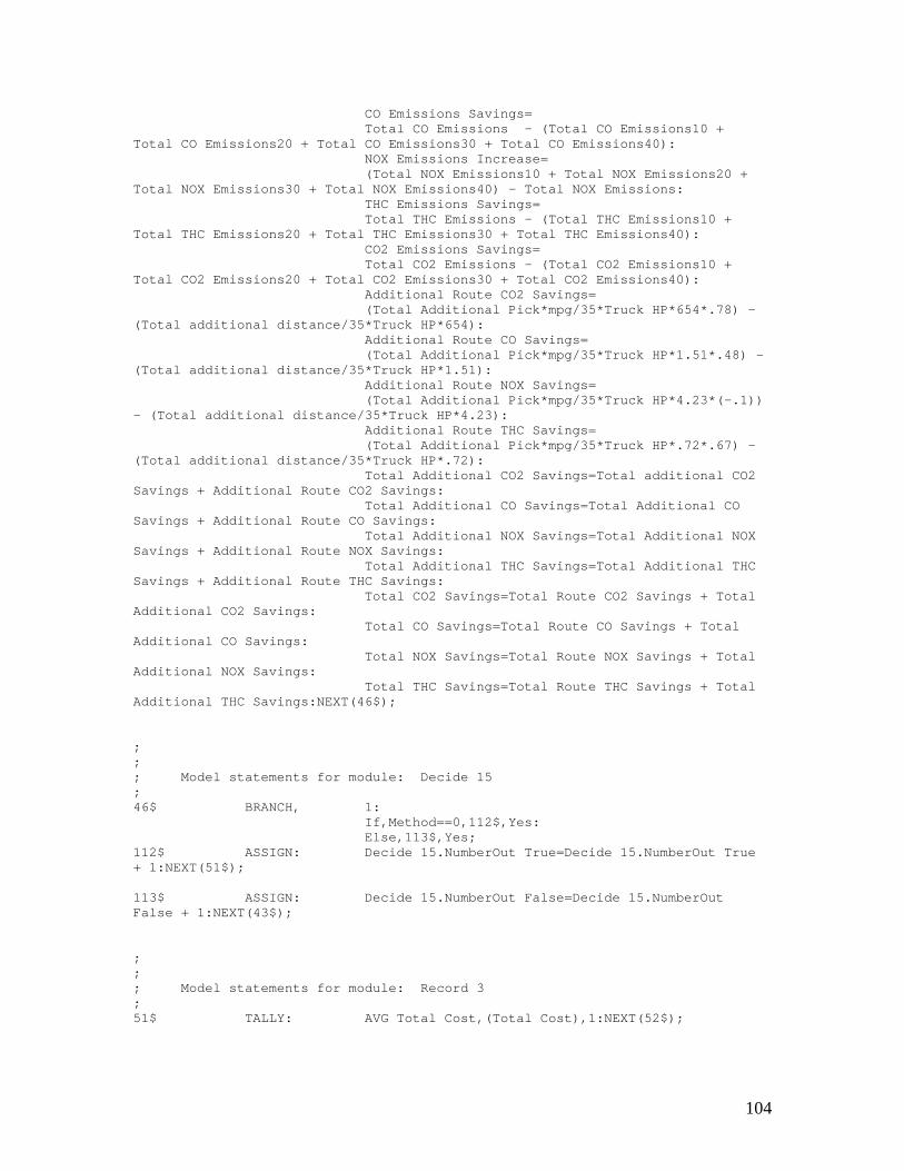
CO Emissions Savings= Total CO Emissions - (Total CO Emissions10 + Total CO Emissions20 + Total CO Emissions30 + Total CO Emissions40): NOX Emissions Increase= (Total NOX Emissions10 + Total NOX Emissions20 + Total NOX Emissions30 + Total NOX Emissions40) - Total NOX Emissions: THC Emissions Savings= Total THC Emissions - (Total THC Emissions10 + Total THC Emissions20 + Total THC Emissions30 + Total THC Emissions40): CO2 Emissions Savings= Total CO2 Emissions - (Total CO2 Emissions10 + Total CO2 Emissions20 + Total CO2 Emissions30 + Total CO2 Emissions40): Additional Route CO2 Savings= (Total Additional Pick*mpg/35*Truck HP*654*.78) - (Total additional distance/35*Truck HP*654): Additional Route CO Savings= (Total Additional Pick*mpg/35*Truck HP*1.51*.48) - (Total additional distance/35*Truck HP*1.51): Additional Route NOX Savings= (Total Additional Pick*mpg/35*Truck HP*4.23*(-.1)) - (Total additional distance/35*Truck HP*4.23): Additional Route THC Savings= (Total Additional Pick*mpg/35*Truck HP*.72*.67) - (Total additional distance/35*Truck HP*.72): Total Additional CO2 Savings=Total additional CO2 Savings + Additional Route CO2 Savings: Total Additional CO Savings=Total Additional CO Savings + Additional Route CO Savings: Total Additional NOX Savings=Total Additional NOX Savings + Additional Route NOX Savings: Total Additional THC Savings=Total Additional THC Savings + Additional Route THC Savings: Total CO2 Savings=Total Route CO2 Savings + Total Additional CO2 Savings: Total CO Savings=Total Route CO Savings + Total Additional CO Savings: Total NOX Savings=Total Route NOX Savings + Total Additional NOX Savings: Total THC Savings=Total Route THC Savings + Total Additional THC Savings:NEXT(46$); ; ; ; Model statements for module: Decide 15 ; 46$ BRANCH, 1: If,Method==0,112$,Yes: Else,113$,Yes; 112$ ASSIGN: Decide 15.NumberOut True=Decide 15.NumberOut True + 1:NEXT(51$); 113$ ASSIGN: Decide 15.NumberOut False=Decide 15.NumberOut False + 1:NEXT(43$); ; ; ; Model statements for module: Record 3 ; 51$ TALLY: AVG Total Cost,(Total Cost),1:NEXT(52$);
104

; ; ; Model statements for module: Record 4 ; 52$ TALLY: Avg Biodiesel Savings,Potential Biodiesel Savings,1:NEXT(55$); ; ; ; Model statements for module: Record 7 ; 55$ TALLY: Cost after Savings,Total Cost - Potential Biodiesel Savings,1:NEXT(53$); ; ; ; Model statements for module: Record 5 ; 53$ TALLY: WCO collected,Total Pick,1:NEXT(54$); ; ; ; Model statements for module: Record 6 ; 54$ TALLY: CO Emissions,CO Emissions Savings,1:NEXT(58$); ; ; ; Model statements for module: Record 8 ; 58$ TALLY: THC Savings,THC Emissions Savings,1:NEXT(59$); ; ; ; Model statements for module: Record 9 ; 59$ TALLY: CO2 Savings Tonnes,CO2 Emissions Savings/(1000*1000),1:NEXT(60$); ; ; ; Model statements for module: Record 10 ; 60$ TALLY: NOX Increase,NOX Emissions Increase,1:NEXT(61$); ; ; ; Model statements for module: Record 11 ; 61$ TALLY: Trucks fueled,total biodiesel/(total biodiesel used +1),1:NEXT(69$); ; ; ; Model statements for module: Record 14
105

; 69$ TALLY: biodiesel created,biodiesel,1:NEXT(62$); ; ; ; Model statements for module: Record 13 ; 62$ TALLY: Total biodiesel loop cost,Total Additional Cost,1:NEXT(11$); ; ; ; Model statements for module: Delay 10 ; 11$ DELAY: 1440,,Other:NEXT(57$); ; ; ; Model statements for module: Route 32 ; 57$ ROUTE: 0.000000000000000,Routing; ; ; ; Model statements for module: Decide 14 ; 43$ BRANCH, 1: If, Total Time < Max Time && Total Additional Cost < Potential Biodiesel Savings && RemCap >= 0, 114$,Yes: Else,115$,Yes; 114$ ASSIGN: Decide 14.NumberOut True=Decide 14.NumberOut True + 1:NEXT(44$); 115$ ASSIGN: Decide 14.NumberOut False=Decide 14.NumberOut False + 1:NEXT(45$); ; ; ; Model statements for module: Record 1 ; 44$ COUNT: Good,1:NEXT(51$); ; ; ; Model statements for module: Record 2 ; 45$ COUNT: Bad,1:NEXT(51$); ; ; ; Model statements for module: Assign 41 ; 24$ ASSIGN: Route CO Emissions10=(Truck HP)*(Distance/35)*(1.43):
106

Route NOX Emissions10=(Truck HP)*(Distance/35)*(4.38): Route THC Emissions10=(Truck HP)*(Distance/35)*(.63): Route CO2 Emissions10= ((Truck HP)*(Distance/35)*(657)) - ((Truck HP)*(Distance/35)*(657)*(.10)*(.78)): Total CO Emissions10=Total CO Emissions10 + Route CO Emissions10: Total NOX Emissions10=Total NOX Emissions10 + Route NOX Emissions10: Total THC Emissions10=Total THC Emissions10 + Route THC Emissions10: Total CO2 Emissions10=Total CO2 Emissions10 + Route CO2 Emissions10:NEXT(25$); ; ; ; Model statements for module: Assign 40 ; 23$ ASSIGN: Route CO Emissions20=(Truck HP)*(distance/35)*(1.32): Route NOX Emissions20=(Truck HP)*(Distance/35)*(4.46): Route THC Emissions20=(Truck HP)*(Distance/35)*(.56): Route CO2 Emissions20= ((Truck HP)*(Distance/35)*(657)) - ((Truck HP)*(Distance/35)*(657)*(.20)*(.78)): Total CO Emissions20=Total CO Emissions20 + Route CO Emissions20: Total NOX Emissions20=Total NOX Emissions20 + Route NOX Emissions20: Total THC Emissions20=Total THC Emissions20 + Route THC Emissions20: Total CO2 Emissions20=Total CO2 Emissions20 + Route CO2 Emissions20:NEXT(25$); ; ; ; Model statements for module: Assign 39 ; 22$ ASSIGN: Route CO Emissions30=(Truck HP)*(Distance/35)*(1.14): Route NOX Emissions30=(Truck HP)*(Distance/35)*(4.8): Route THC Emissions30=(Truck HP)*(Distance/35)*(.54): ROute CO2 Emissions30= ((Truck HP)*(Distance/35)*(685)) - ((Truck HP)*(Distance/35)*(685)*(.30)*(.78)): Total CO Emissions30=Total CO Emissions30 + Route CO Emissions30: Total NOX Emissions30=Total NOX Emissions30 + Route NOX Emissions30: Total THC Emissions30=Total THC Emissions30 + Route THC Emissions30: Total CO2 Emissions30=Total CO2 Emissions30 + Route CO2 Emissions30:NEXT(25$);
107

; ; ; Model statements for module: Assign 38 ; 21$ ASSIGN: Route CO Emissions40=(Truck HP)*(Distance/35)*(1.07): Route NOX Emissions40=(Truck HP)*(Distance/35)*(4.86): Route THC Emissions40=(Truck HP)*(Distance/35)*(.43): Route CO2 Emissions40= ((Truck HP)*(Distance/35)*(684)) - ((Truck HP)*(Distance/35)*(684)*(.40)*(.78)): Total CO Emissions40=Total CO Emissions40 + Route CO Emissions40: Total NOX Emissions40=Total NOX Emissions40 + Route NOX Emissions40: Total THC Emissions40=Total THC Emissions40 + Route THC Emissions40: Total CO2 Emissions40=Total NOX Emissions40 + Route NOX Emissions40:NEXT(25$); ; ; ; Model statements for module: Station 16 ; 6$ STATION, Stop 2; 118$ DELAY: 0.0,,VA:NEXT(8$); ; ; ; Model statements for module: Assign 19 ; 8$ ASSIGN: Drop AMnt=1.26e+004 + 7.67e+004 * BETA(0.404, 1.25): RemCap=REmCap+Drop Amnt: Time in route=Time in route + ((((Stop Location - previous stop location)/35)*60)+delay time): Total Drop Time=Total Drop Time + delay Time: Total time=Total Time + Delay Time: previous stop location=Stop Location:NEXT(65$); ; ; ; Model statements for module: Decide 20 ; 65$ BRANCH, 1: If,Time in route <= Max Time,119$,Yes: Else,120$,Yes; 119$ ASSIGN: Was delivery late? 2.NumberOut True=Was delivery late? 2.NumberOut True + 1:NEXT(7$); 120$ ASSIGN: Was delivery late? 2.NumberOut False=Was delivery late? 2.NumberOut False + 1:NEXT(66$); ; ; ; Model statements for module: Route 17
108

; 7$ ROUTE: 0,Dispatch; ; ; ; Model statements for module: Assign 45 ; 66$ ASSIGN: Number late=Number late + 1:NEXT(7$); ; ; ; Model statements for module: Station 17 ; 9$ STATION, Stop 3; 123$ DELAY: 0.0,,VA:NEXT(18$); ; ; ; Model statements for module: Assign 35 ; 18$ ASSIGN: Additional Distance=UNIF(0,Added Distance Per Stop): Total Additional Distance=Total Additional Distance + Additional Distance: Additional Time=(((Added Distance Per Stop)/35)*60) + Delay time: Time in route=Time in route + additional time: Total Additional Time=Total Additional Time + Additional Time:NEXT(71$); ; ; ; Model statements for module: Assign 47 ; 71$ ASSIGN: Additional Pick=min((RemCap*.004329), UNIF(16, 23)): Number of containers=additional pick/5: RemCap=RemCap-(number of containers*(5*231)): Total Additional Pick=Total Additional Pick + Additional Pick: Total Pick=total pick + Additional Pick: Total time=Total Time + Additional Time: Cumulative Additional Time=Cumulative Additional Time + Additional Time:NEXT(28$); ; ; ; Model statements for module: Route 26 ; 28$ ROUTE: 0.000000000000000,Dispatch; ; ; ; Model statements for module: Station 19 ;
109

36$ STATION, Dispatch; 126$ DELAY: 0.0,,VA:NEXT(67$); ; ; ; Model statements for module: Decide 21 ; 67$ BRANCH, 1: If,Number of Stops Made==0,127$,Yes: Else,128$,Yes; 127$ ASSIGN: Decide 21.NumberOut True=Decide 21.NumberOut True + 1:NEXT(38$); 128$ ASSIGN: Decide 21.NumberOut False=Decide 21.NumberOut False + 1:NEXT(68$); 38$ ASSIGN: Number of Stops Made=Number of Stops Made + 1; 34$ FINDJ, 1,Number of Stops + Number of Stop 3:Min(DD(J,1)); 35$ ASSIGN: Stop Location=DD(J,1): Stop Type=DD(J,2):NEXT(42$); ; ; ; Model statements for module: Decide 13 ; 42$ BRANCH, 1: If,Number of Stops Made>Number of Stops + Number of stop 3 + 1,129$,Yes: Else,130$,Yes; 129$ ASSIGN: Decide 13.NumberOut True=Decide 13.NumberOut True + 1:NEXT(41$); 130$ ASSIGN: Decide 13.NumberOut False=Decide 13.NumberOut False + 1:NEXT(37$); ; ; ; Model statements for module: Route 29 ; 41$ ROUTE: 0.000000000000000,Warehouse; ; ; ; Model statements for module: Decide 12 ; 37$ BRANCH, 1: If,Stop Type==1,4$,Yes: If,Stop Type==2,39$,Yes: Else,40$,Yes; ; ; ; Model statements for module: Route 28 ; 40$ ROUTE: 0.000000000000000,Stop 3; ; ;
110

; Model statements for module: Route 15 ; 4$ ROUTE: 0,Stop 1; ; ; ; Model statements for module: Route 27 ; 39$ ROUTE: 0.000000000000000,Stop 2; 68$ ASSIGN: Number of Stops Made=Number of Stops Made + 1: DD(J,1)=100*Max time:NEXT(34$); ; ; ; Model statements for module: Create 2 ; 133$ CREATE, 1,MinutesToBaseTime(TFIN),Entity 1:MinutesToBaseTime(TFIN),1:NEXT(134$); 134$ ASSIGN: Create 2.NumberOut=Create 2.NumberOut + 1:NEXT(72$); ; ; ; Model statements for module: ReadWrite 1 ; 72$ WRITE, biodiesel data: Total Cost - Potential Biodiesel savings:NEXT(74$); ; ; ; Model statements for module: ReadWrite 2 ; 74$ WRITE, CO2 data: Total CO2 Savings:NEXT(75$); ; ; ; Model statements for module: ReadWrite 3 ; 75$ WRITE, CO data: Total CO Savings:NEXT(76$); ; ; ; Model statements for module: ReadWrite 4 ; 76$ WRITE, NOX Data: Total NOX Savings:NEXT(77$); ; ; ; Model statements for module: ReadWrite 5
111
112
; 77$ WRITE, THC Data: Total THC Savings:NEXT(78$); ; ; ; Model statements for module: ReadWrite 6 ; 78$ WRITE, Trucks Data: Total biodiesel/(total biodiesel used):NEXT(79$); ; ; ; Model statements for module: ReadWrite 7 ; 79$ WRITE, Number late data: Number late:NEXT(73$); ; ; ; Model statements for module: Dispose 1 ; 73$ ASSIGN: Dispose 1.NumberOut=Dispose 1.NumberOut + 1; 137$ DISPOSE: Yes;