Economic Analysis of Stage I of the California WaterFix · Economic Analysis of Stage I of the ... The analysis described in this report concludes that Stage I of the California WaterFix

Economic Analysis of Stage I of the California WaterFix Costs and Benefits to Urban and Agricultural Participants

PREPARED FOR

California Department of Water Resources

PREPARED BY

David L. Sunding, Ph.D.

February 12, 2018

This report was prepared for the California Department of Water Resources. All results and any errors are the responsibility of the authors and do not represent the opinion of The Brattle Group or its clients.

Acknowledgement: We acknowledge the valuable contributions of many individuals to this report and to the underlying analysis, including members of The Brattle Group for peer review.

Copyright © 2018 The Brattle Group, Inc.

i | brattle.com

Table of Contents

I. Introduction and Summary of Findings ........................................................................................ 1

II. WaterFix Project ........................................................................................................................... 2

III. Cost Allocation and Financing ..................................................................................................... 2

IV. Project Yields ............................................................................................................................... 3

V. Water Supply Benefits to Urban Areas ........................................................................................ 8

VI. Water Supply Benefits to Agricultural Water Users .................................................................. 12

VII. Water Quality Benefits ............................................................................................................... 20

VIII. Earthquake Reliability ................................................................................................................ 21

IX. Climate Change Mitigation ........................................................................................................ 29

X. Quantified Benefits and Costs to State Water Contractors ......................................................... 30

1 | brattle.com

I. Introduction and Summary of Findings

The California WaterFix, considered initially as part of the Bay Delta Conservation Plan, is a

foundational component of the state’s Water Action Plan. It addresses environmental, seismic,

water quality and climate change threats to the existing water conveyance infrastructure in the

Delta and complements efforts to improve ecological functions being advanced by the state’s

California EcoRestore program.

During this planning process that now spans more than 11 years, economic principles for

measuring costs and benefits have been applied over time in various reports to review the values

of water system and ecosystem improvements and to help advance public discussion and debate.

Such cost-benefit analyses have gone beyond what is legally required because of the statewide

significance of the project. This most recent analysis is intended to help examine the evolved

project and the related costs and benefits of the potential participants in both the urban and

agricultural sectors.

After several years of analysis, the California Department of Water Resources is considering an

option to implement the California WaterFix project in two Stages. Stage I would consist of two

3,000-cfs intakes connected to one 40-ft diameter tunnel. From the intakes, water would be

conveyed by gravity flow to a 6,000-cfs pumping plant that lifts it into Clifton Court Forebay.

Stage II of the California WaterFix would consist of an additional 3,000-cfs intake connected to a

second tunnel.

Because not all aspects of financing and project participation have been decided at present, this

report considers Stage I costs and benefits in multiple alternative scenarios. These scenarios

include whether i) low-interest federal financing will be available to cover a share of project

costs, ii) revenues will be collected for federal contractors’ use of up to 1,000-cfs of the Stage I

project or whether the State Water Contractors will make use of the entire capacity, and iii)

trading of project capacity will be allowed among the State Water Contractors. Participants in

Stage II of the California WaterFix are not currently known. Depending on the evolution of

environmental regulations, water demands and climate, state and federal water agencies may

decide to implement Stage II at some point in the future. At that time, a detailed cost-benefit

analysis of Stage II can be completed.

2 | brattle.com

The analysis described in this report concludes that Stage I of the California WaterFix passes a

cost-benefit test for SWP urban and agricultural agencies under all scenarios analyzed. The

ability of project participants to trade their shares in the project is highly beneficial to SWP

agricultural agencies, as is the availability of federal low-interest financing. The analysis also

indicates that federal contractors south of the Delta receive benefits in excess of costs from the

use of up to 1,000-cfs of Stage 1 project capacity. The State Water Project contractors would also

receive positive net benefits were they to use all 6,000-cfs of capacity.

II. WaterFix Project

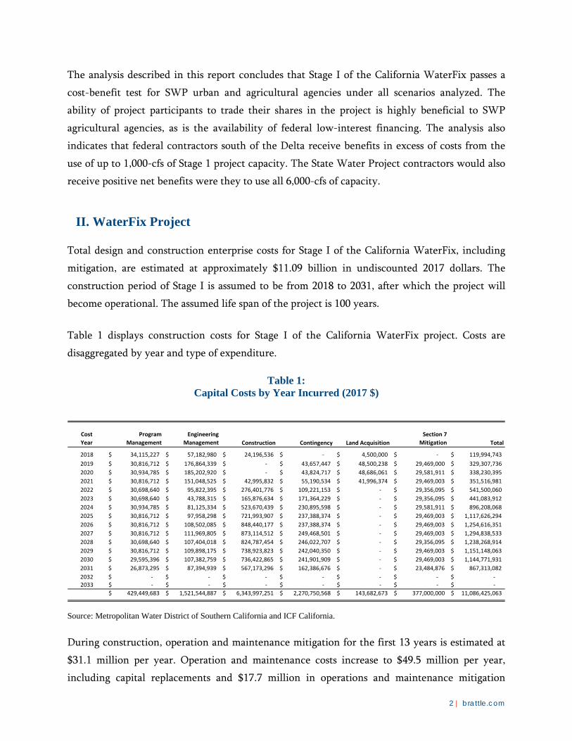
Total design and construction enterprise costs for Stage I of the California WaterFix, including

mitigation, are estimated at approximately $11.09 billion in undiscounted 2017 dollars. The

construction period of Stage I is assumed to be from 2018 to 2031, after which the project will

become operational. The assumed life span of the project is 100 years.

Table 1 displays construction costs for Stage I of the California WaterFix project. Costs are

disaggregated by year and type of expenditure.

Table 1: Capital Costs by Year Incurred (2017 $)

Source: Metropolitan Water District of Southern California and ICF California.

During construction, operation and maintenance mitigation for the first 13 years is estimated at

$31.1 million per year. Operation and maintenance costs increase to $49.5 million per year,

including capital replacements and $17.7 million in operations and maintenance mitigation

Cost Year

Program Management

EngineeringManagement Construction Contingency Land Acquisition

Section 7 Mitigation Total

2018 34,115,227$ 57,182,980$ 24,196,536$ -$ 4,500,000$ -$ 119,994,743$ 2019 30,816,712$ 176,864,339$ -$ 43,657,447$ 48,500,238$ 29,469,000$ 329,307,736$ 2020 30,934,785$ 185,202,920$ -$ 43,824,717$ 48,686,061$ 29,581,911$ 338,230,395$ 2021 30,816,712$ 151,048,525$ 42,995,832$ 55,190,534$ 41,996,374$ 29,469,003$ 351,516,981$ 2022 30,698,640$ 95,822,395$ 276,401,776$ 109,221,153$ -$ 29,356,095$ 541,500,060$ 2023 30,698,640$ 43,788,315$ 165,876,634$ 171,364,229$ -$ 29,356,095$ 441,083,912$ 2024 30,934,785$ 81,125,334$ 523,670,439$ 230,895,598$ -$ 29,581,911$ 896,208,068$ 2025 30,816,712$ 97,958,298$ 721,993,907$ 237,388,374$ -$ 29,469,003$ 1,117,626,294$ 2026 30,816,712$ 108,502,085$ 848,440,177$ 237,388,374$ -$ 29,469,003$ 1,254,616,351$ 2027 30,816,712$ 111,969,805$ 873,114,512$ 249,468,501$ -$ 29,469,003$ 1,294,838,533$ 2028 30,698,640$ 107,404,018$ 824,787,454$ 246,022,707$ -$ 29,356,095$ 1,238,268,914$ 2029 30,816,712$ 109,898,175$ 738,923,823$ 242,040,350$ -$ 29,469,003$ 1,151,148,063$ 2030 29,595,396$ 107,382,759$ 736,422,865$ 241,901,909$ -$ 29,469,003$ 1,144,771,931$ 2031 26,873,295$ 87,394,939$ 567,173,296$ 162,386,676$ -$ 23,484,876$ 867,313,082$ 2032 -$ -$ -$ -$ -$ -$ -$ 2033 -$ -$ -$ -$ -$ -$ -$

429,449,683$ 1,521,544,887$ 6,343,997,251$ 2,270,750,568$ 143,682,673$ 377,000,000$ 11,086,425,063$

3 | brattle.com

annually, for the first 50 years of the project. Thereafter, the operation and maintenance costs

amount to $31.9 million per year.

III. Cost Allocation and Financing

At present, it is expected that on a long-term average basis the State Water Contractors would

utilize 5,000-cfs of the 6,000-cfs of total Stage I capacity. The remaining up to 1,000-cfs would be

available for use by Central Valley Project south of Delta contractors and other entities receiving

Central Valley Project deliveries. The exact mechanism for funding the 1,000-cfs of capacity

potentially used by the federal contractors has not been determined. This report accordingly

analyzes two scenarios, one in which the State Water Contractors pay for and utilize 5,000-cfs of

project capacity, and one in which they finance and utilize the entire 6,000-cfs. Costs and

benefits to the State Water Contractors are the primary focus of the analysis, and benefits to

federal contractors from their use of 1,000-cfs of project capacity are analyzed separately.

Some State Water Contractors have indicated that they do not need the benefit of the California

WaterFix and do not wish to pay for it. This position is consistent with the analysis of

agricultural benefits presented in this report. There is active discussion among the State Water

Contractors about allowing agencies to transfer their costs and benefits to other Contractors. In

such an arrangement, a water agency that does not wish to participate in Stage 1 of the WaterFix

could transfer their share of costs to another agency; the selling agency would then receive water

supplies equal to the future baseline defined in this report. To account for the possibility that

project capacity could be traded among the State Water Contractors, this report considers two

scenarios: in one scenario all agencies would participate in the project and pay a share of costs

determined by their Table A allocation; in the alternative scenario, a limited amount of project

benefits and costs would be reallocated from agricultural to urban users.

Financing is another powerful factor that impacts both costs and benefits. This report considers

two possibilities: market-rate financing, and low-interest rate financing that may be available

under a variety of existing and proposed federal laws. Due to the uncertain nature of the

WaterFix funding mechanisms, this report considers several scenarios: financing at market rates,

and low-interest rate federal financing of 50 or 100 percent of the project. This report assumes

for planning purposes that low-interest rate federal funding would carry an interest rate of 200

basis points below the comparable market rate and would have a comparable repayment period.

4 | brattle.com

IV. Project Yields

The State Water Project is the most important source of imported water for the State Water

Contractor agencies included in the analysis. SWP deliveries to these agencies consist of Table A,

Article 21 and Article 56 supplies. Table A supply is a contracted quantity that totals roughly 4.2

MAF per year across all the urban member agencies in the SDBSIM model. Article 21 deliveries

are unscheduled water that is available in wet years, and is essentially the surplus water that

remains after all operational, water quality and Delta requirements are met. Article 56 of the

Water Supply Contracts allows for some carryover water to be held in San Luis Reservoir during

wet years and delivered in the subsequent calendar year.

The Central Valley Project is owned and operated by the Bureau of Reclamation. The CVP

provides deliveries to agricultural and urban water contractors south of the Delta. Some or all of

these CVP contractors, notably Westlands Water District and the Santa Clara Valley Water

District (also a SWP contractor), may decide to participate in Stage I of the California WaterFix

with respect to CVP supplies.

Estimates of future SWP and CVP deliveries under Stage I of the California WaterFix are

forecasted using the CALSIM II model, a generalized water resource simulation model developed

by the California Department of Water Resources and the U.S. Bureau of Reclamation.1 CALSIM

II is a simulation model that uses linear programming to project water deliveries given

hydrological and regulatory constraints and user priority weights. Data produced using CALSIM

II are used to estimate the water to be exported from the Delta and distributed to the south of

Delta State Water Project contractors under the following scenarios:

• California WaterFix2

• Existing Conveyance with California WaterFix Operating Criteria

The benefits and costs of Stage I of Califonia WaterFix must be evaluated in relation to the future

baseline conditions that would likely occur if a new water conveyance system were not built.

The future baseline conditions are not static and they take into account past, present, and

anticipated future regulatory constraints on the operations of the existing Delta water

1 The CalSim II model did not consider the possibility of transfers between water agencies in its analysis. 2 Stage I WaterFix operations are assumed to be the H3+ (NOD) 5000 SWP-1000 CVP model run. Sensitivity

analysis was also performed using the H3+ (NOD) 6000 SWP model run.

5 | brattle.com

conveyance system. Past regulatory constraints that affect the current existing water conveyance

system include the “Reasonable and Prudent Alternatives” (RPA) contained in the biological

opinions for the “Coordinated Long-term Operations of the CVP and SWP” issued by the U.S.

Fish and Wildlife Service (FWS) in 2008 and the National Marine Fisheries Service (NMFS) in

2009. Other actions required by existing regulatory authorizations are described in the Bay Delta

Conservation Plan/California WaterFix Final Environmental Impact Report/Environmental

Impact Statement (December 2016) (EIR/EIS).3 Future conditions that factor into the baseline

conditions include projected climate conditions and additional regulatory constraints that could

apply to the existing water conveyance system.

The RPA4 contained in the biological opinions for the Coordinated Long-Term Operations of the

CVP and SWP issued by the FWS and NMFS require a wide range of actions. They include

habitat restoration, complex export restrictions in the Delta, additional upstream storage and

flow requirements, new research, and monitoring. Also required are several restrictions on south

Delta pumping, requirements to improve pre-screen losses at Clifton Court Forebay, a prescribed

fall season outflow in wet and above normal rainfall years, Delta and Yolo Bypass restoration

actions, a suite of monitoring and research actions, and a suite of upstream actions, among other

requirements. In addition, the baseline conditions reflect the implementation of the terms and

conditions of the State Incidental Take Permit for SWP Operations for Longfin Smelt, which are

generally consistent with the biological opinions for the Coordinated Long-term Operations of

the CVP and SWP, and the notch in the Fremont Weir that is included in NMFS’ biological

opinion for the Yolo Bypass restoration. The implementation of these regulatory actions is

included in the baseline conditions used to assess the benefits and cost of the off-site and on-site

alternatives.

Notwithstanding these operational measures, the baseline conditions reflect the expectation that

further constraints would be placed on the SWP and CVP operations. Data has shown that fish

species continue to decline in the Delta for a variety of reasons, including the recent extreme

3 More information about past environmental and regulatory constraints that affect the baseline

conditions of the existing water conveyance system is provided in Chapter 3 of the EIR/EIS and Appendix 3D and Appendix 5A to the EIR/EIS. The EIR/EIS is available at http://baydeltaconservationplan.com/FinalEIREIS/FinalEIR-EIS_VolumeI.aspx.

4 The RPAs must be implemented to avoid jeopardizing the continued existence of species subject to the federal Endangered Species Act (ESA) and to maintain authorization to “take” those species pursuant to the ESA.

http://baydeltaconservationplan.com/FinalEIREIS/FinalEIR-EIS_VolumeI.aspx

6 | brattle.com

five-year drought, even with the implementation of these regulatory actions.5 For example, the

decline of the Delta smelt and winter-run Chinook salmon has been well-documented before

(Pelagic Organism Decline [POD] and NMFS Species Report Cards) and throughout the drought

by various state and federal agencies.6

As evidenced by the 2008 and 2009 biological opinions for the Coordinated Long-Term

Operations of the CVP and SWP, regardless of the reasons for decline, the historical regulatory

pattern for addressing these declines has been to increasingly constrain water deliveries,

including Delta operations and cold water pool storage, to maintain greater flows and improved

habitat conditions for fish. Discussions during the development of the California WaterFix

project, the Bureau of Reclamation’s request to reinitiate consultation for the Coordinated Long-

Term Operations of the CVP and SWP, and ongoing planning efforts (such as the Bay-Delta

Water Quality Control Plan Update) all indicate this regulatory pattern would likely continue.

The baseline conditions therefore also reflect likely future regulatory constraints, described

below, that would be applied to south Delta operations under the current water conveyance

system.

New regulatory constraints on water deliveries, known as Scenario 6 Old and Middle River

(Scenario 6 OMR) criteria, are designed to preserve the reduced reverse flow conditions. These

constraints are assumed to be required. The Scenario 6 OMR criteria would further constrain

water exports from the south Delta during wetter years as compared to the existing biological

opinions. Modifications to the head of Old River Gate and changes in its operation are also

assumed. These changes would include a permanent operable gate to replace the temporary rock

barrier located there. The permanent head of Old River Gate would be operated January through

June to promote fish migration, which would affect water quality and water supply compared to

the existing rock barrier.7

5 Fish surveys conducted by the California Department of Fish and Wildlife are available at http://www.dfg.ca.gov/delta/data/. 6 The POD and more information regarding NMFS’ data are available at http://www.science.calwater.ca.gov/pod/pod_index.html and http://www.nmfs.noaa.gov/pr/species/Species%20in%20the%20Spotlight/sacramento_winter-run_chinook_salmon_spotlight_species_5-year_action_plan_final_jan_25_2016__1_.pdf. 7 State and federal wildlife agencies have indicated the Scenario 6 OMR criteria and head of Old River permanent operable gate is assumed to be included in an amended biological opinion for the for the Coordinated Long-term Operations of the CVP and SWP or other regulatory authorizations, and

Continued on next page

http://www.dfg.ca.gov/delta/data/

http://www.science.calwater.ca.gov/pod/pod_index.html

http://www.nmfs.noaa.gov/pr/species/Species%20in%20the%20Spotlight/sacramento_winter-run_chinook_salmon_spotlight_species_5-year_action_plan_final_jan_25_2016__1_.pdf

http://www.nmfs.noaa.gov/pr/species/Species%20in%20the%20Spotlight/sacramento_winter-run_chinook_salmon_spotlight_species_5-year_action_plan_final_jan_25_2016__1_.pdf

7 | brattle.com

In addition to the Scenario 6 OMR criteria and changes to the head of Old River Gate, further

restrictions on the existing long-term SWP and CVP operations are assumed to result from

amendments to the existing biological opinions. In its request to reinitiate consultation with the

FWS and NMFS, the Bureau of Reclamation expects the consultation will update the system-

wide operating criteria and review the existing RPAs to determine their “continued substance

and efficacy in meeting the requirements of Section 7 of the ESA.” Based on current species

status, recent drought conditions, improved climate change projections, the scope of the Bureau

of Reclamation’s request to reinitiate consultation, ongoing discussions about outflows and in-

stream flows, and the historical trend of regulation, it is likely these consultations would result in

further restrictions on SWP and CVP operations. Likewise, the State Water Resources Control

Board is currently in the process of updating the Bay-Delta Water Quality Control Plan, and

based on the Stage 1 and 2 reports released to date,8 and the ongoing negotiated resolutions to

increase environmental flows in the Sacramento and San Joaquin rivers, it is assumed that the

Plan would further constrain water supplies from the south Delta.

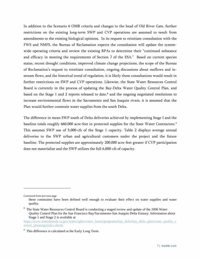
The difference in mean SWP south of Delta deliveries achieved by implementing Stage I and the

baseline totals roughly 660,000 acre-feet in protected supplies for the State Water Contractors.9

This assumes SWP use of 5,000-cfs of the Stage 1 capacity. Table 2 displays average annual

deliveries to the SWP urban and agricultural customers under the project and the future

baseline. The protected supplies are approximately 200,000 acre-feet greater if CVP participation

does not materialize and the SWP utilizes the full 6,000-cfs of capacity.

Continued from previous page these constraints have been defined well enough to evaluate their effect on water supplies and water quality. 8 The State Water Resources Control Board is conducting a staged review and update of the 2006 Water Quality Control Plan for the San Francisco Bay/Sacramento-San Joaquin Delta Estuary. Information about Stage 1 and Stage 2 is available at https://www.waterboards.ca.gov/waterrights/water_issues/programs/bay_delta/bay_delta_plan/water_quality_control_planning/index.shtml. 9 This difference is calculated at the Early Long Term.

https://www.waterboards.ca.gov/waterrights/water_issues/programs/bay_delta/bay_delta_plan/water_quality_control_planning/index.shtml

https://www.waterboards.ca.gov/waterrights/water_issues/programs/bay_delta/bay_delta_plan/water_quality_control_planning/index.shtml

8 | brattle.com

Table 2: Average Annual Yields for

State Water Project and Central Valley Project Agencies

Source: CH2M Hill.

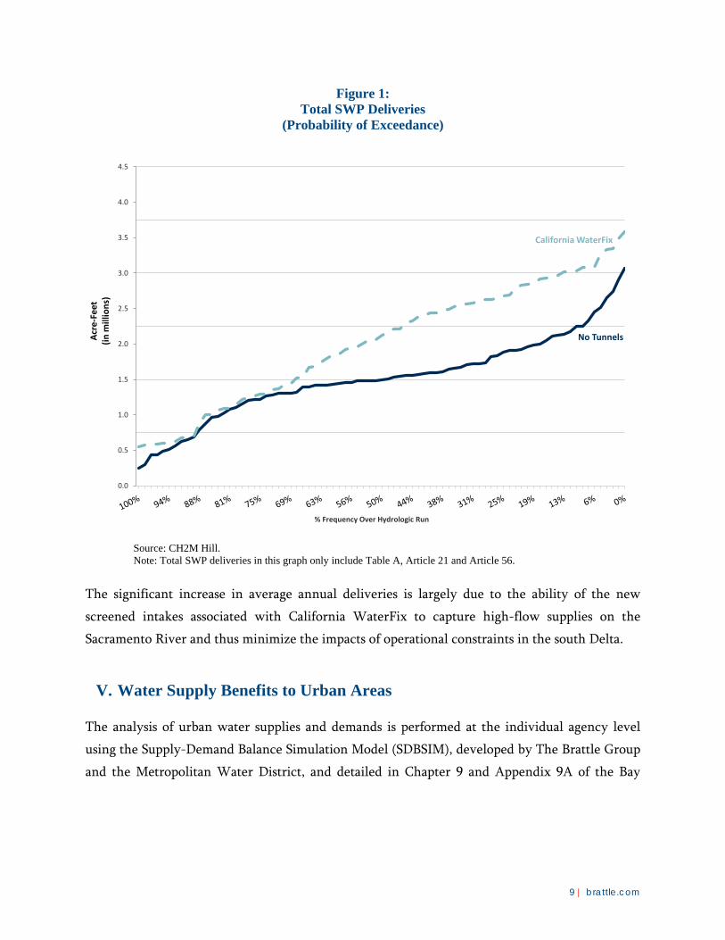
Of course, mean deliveries are not sufficient to calculate project benefits. In addition to the

incremental supply created by the project, it is important to take account of when this

incremental supply is created (i.e., between wet and dry years). Figure 1 displays exceedance

curves for SWP deliveries under Stage I and in the baseline. The CALSIM II runs indicate that

the incremental water supplies produced by Stage I are available primarily in average to wet

years. This pattern of incremental supplies is important since agencies with adequate storage are

better able to utilize the enhanced wet-year deliveries and hence receive larger benefits from

Stage I, all else equal.

9 | brattle.com

Figure 1: Total SWP Deliveries

(Probability of Exceedance)

Source: CH2M Hill. Note: Total SWP deliveries in this graph only include Table A, Article 21 and Article 56.

The significant increase in average annual deliveries is largely due to the ability of the new

screened intakes associated with California WaterFix to capture high-flow supplies on the

Sacramento River and thus minimize the impacts of operational constraints in the south Delta.

V. Water Supply Benefits to Urban Areas

The analysis of urban water supplies and demands is performed at the individual agency level

using the Supply-Demand Balance Simulation Model (SDBSIM), developed by The Brattle Group

and the Metropolitan Water District, and detailed in Chapter 9 and Appendix 9A of the Bay

No Tunnels

California WaterFix

0.0

0.5

1.0

1.5

2.0

2.5

3.0

3.5

4.0

4.5

Acre

-Fee

t(in

mill

ions

)

% Frequency Over Hydrologic Run

10 | brattle.com

Delta Conservation Plan.10 The SDBSIM is a probabilistic water portfolio simulation model that

apportions and values shortages at the agency level for 36 major urban agencies receiving Delta

water supplies directly or indirectly.11 These agencies were chosen for analysis because they

receive the bulk of SWP urban deliveries and because they have the largest potential to

experience changes in welfare as a result of variations in Delta yields. Some of these agencies are

members of the Metropolitan Water District of Southern California (MWD), which receives

roughly half of all available yields from the SWP.

Many of the 36 agencies represented in the SDBSIM are wholesalers themselves. For these

agencies, it is necessary to model demand and supply conditions in the retail agencies they serve.

Extending the number of agencies modeled to include the wholesale customers, the SDBSIM

actually covers over 200 retail water agencies throughout California. This level of disaggregation

captures real-world variation in water rates among utilities. Further, because different water

retailers have different water supply portfolios, a given change in SWP deliveries can translate

into different degrees of shortage across water agencies.

Water shortages following a supply disruption have the potential to adversely affect economic

outcomes among several types of water users, including agricultural, residential, industrial,

commercial and government water users. The SDBSIM considers a drought response framework

in which water supply reductions are distributed among the users according to their unit value of

water. Losses due to shortages, and correspondingly benefits due to avoided shortages, are

measured by computing consumer willingness to pay to avoid water service interruptions in each

sector.

Future hydrologic conditions are uncertain. Due to discounting of project benefits, the timing of

future droughts may have a significant effect on the value of infrastructure that improves water

supply reliability. The advantage of SDBSIM’s indexed sequential Monte Carlo simulation

method is that it can account for supply uncertainty by considering 81 different sets of forecasted

hydrologic time series data and the corresponding supply availability. As suggested earlier, each

10 http://baydeltaconservationplan.com/Library/ArchivedDocuments/BDCPAdminDraft2013.aspx 11 The SDBSIM currently incorporates the 26 MWD member agencies along with Alameda County Water

District, Antelope Valley-East Kern Water Agency, Castaic Lake Water Agency, City of Santa Maria, Mojave Water Agency, Palmdale Water District, San Bernardino Valley Municipal Water District, San Gorgonio Pass Water Agency and Zone 7.

http://baydeltaconservationplan.com/Library/ArchivedDocuments/BDCPAdminDraft2013.aspx

11 | brattle.com

time series of supply data represents a possible draw from historical hydrological conditions. For

example, one SDBSIM simulation uses as input the annual hydrologic conditions from 1922 to

1960. Another SDBSIM simulation uses inputs from 1923 to 1961. In subsequent simulations,

each year from 1922 to 2002 is considered as the starting year to initialize supply conditions in

2031.12 In this way, water supply availability between 2031 and 2130 is computed under a wide

range of potential hydrologic conditions. Thus, the model produces probabilistic water supply

availability given a distribution of potential hydrologic conditions, while also having the ability

to predict supply under certain hydrologic conditions.

The first step in valuing the urban water supply benefits of Stage I of the California WaterFix is

to identify patterns of urban water shortages under the proposed project relative to those

occurring in the future baseline scenario. To project these shortage patterns, all other water

supplies available to the project participants must be accounted for. In general, water supplies

available to these agencies consist of both local and imported supplies. Local supplies are

composed of groundwater, groundwater recovery, local surface water, recycled water,

desalinated seawater and water from the Los Angeles Aqueduct. Imported supplies for Southern

California come from the Colorado River and the SWP. The major sources of imported water for

the portions of the Bay Area included in the analysis come from the San Francisco Public

Utilities Commission Regional Water System, the CVP and the SWP. Individual agencies may

have other specific import sources; for example, the Zone 7 Water Agency in Alameda County

receives imported water from Byron Bethany Irrigation District.

Water demand is projected individually for each of the 36 urban agencies included in the

SDBSIM using disaggregated econometric models, which capture the impacts of long-term

socioeconomic trends on retail demands at the water agency level.13 These models incorporate

economic and demographic projections that are either forecasted by the agencies themselves or

provided by the regional planning agencies, the Southern California Association of Governments

12 The ordering of years for historical hydrologic data is preserved because there is dependence in

conditions across years. Hydrologic data does not exist beyond 2002. When a simulation requires a time series of hydrologic input data beyond 2002, the time series reverts back to 1922 as the year of hydrologic conditions following 2002.

13 The demands for the MWD agencies are forecasted using the Metropolitan Water District Econometric Demand Model (MWD–EDM) developed by The Brattle Group. Demands for each of the remaining SWP agencies are forecasted by the agencies.

12 | brattle.com

and the San Diego Association of Governments.14 The demand forecasts are adjusted according to

expected implementation of conservation programs by individual water agencies.15

For the service area of the Metropolitan Water District of Southern California specifically, total

water demand is expected to rise from about 3.3 MAF in 2015 to about 3.7 MAF in 2050, or about

8%. Single-family residential and commercial demand is expected to increase by about 3%,

compared to about 30% for multi-family residential demand. While aggregate demand is

projected to increase over the planning horizon, the per capita water demand is anticipated to

drop to under 140 gallons per capita per day. At the same time, water rates are expected to

experience growth over the coming decades. Additionally, aggregate demand is expected to

increase but at a rate below population growth due to changes in household population sizes.

The SDBSIM uses an indexed sequential Monte Carlo simulation method to measure the supply-

demand balance outcomes for forecasted years given the pattern of historical hydrologic

conditions between years 1922 and 2002. It adjusts the demand and supplies of a forecasted year

given hydrologic conditions in past years, then takes the next sequential forecasted year and

adjusts the demand and supplies for that year given conditions in the next sequential historical

hydrologic year, and so on. By preserving the series of climate patterns (i.e., the hydrologic

trace), the model is able to capture the operation of storage resources that are drawn upon and

refilled over the forecast horizon given a probabilistic sequence of hydrologic conditions.

For each year, the SDBSIM compares the forecasted demand to the sum of available projected

local supplies and imported supplies less conservation savings in order to assess the disparity

between the amount of water desired and the amount that can be provided. If a shortage exists,

the SDBSIM may release additional supplies from storage or transfer programs until supply and

demand are balanced or until these supplies are exhausted. A net shortage for the year results if

the gap between supplies and demands is too large to be balanced by storage and transfer

programs. If a surplus exists, the SDBSIM may allocate surplus water to various storage accounts

14 The underlying figures of the 2015 MWD–EDM model, rely on the SCAG’s 2012 Regional Transportation

Plan (RTP-12) and SANDAG’s Series 13 Forecast. 15 The models forecast demand in 5-year intervals for each of the following sectors: unmetered users, single

family residential, multi-family residential and commercial, industrial, & institutional users. Linear interpolations are generated for the interim years; this procedure results in annual forecasts by sector for each of the urban water agencies.

13 | brattle.com

until all storage capacity is used; any remaining surplus supplies are considered unused and are

not available for use in subsequent years of the forecast. Shortages are forecasted for each year in

each agency in the model under the baseline scenarios and under implementation of California

WaterFix. Consistent with the assumption that the proposed project will not yield any additional

deliveries until 2031, there are no avoided shortages prior to that year since deliveries in the

Stage I and baseline cases are the same.

The value of avoiding future water shortages is estimated in SDBSIM through a combination of

economic theory and econometric modeling of urban water demand relationships. These

relationships capture the declining marginal utility of water, which in turn implies greater value

lost per unit of shortage the larger the magnitude of the shortage. Consider residential water use,

for example, which falls into several broader categories, each with a different priority of use. The

willingness to pay for water used for drinking and basic sanitation, for example, is larger than the

willingness to pay for water used for washing cars and outdoor irrigation. Consumer willingness

to pay to avoid a water service interruption therefore rises with the magnitude of the supply

shortage, as consumers are forced to cut more deeply into high-priority uses of water when faced

with larger shortages.

Urban water consumers are faced with a given set of water rates and, given these rates, are

generally free to purchase their desired quantities of water. Prevailing water rates combined with

observed consumption levels provide information about the value of water to households at a

single point on the demand curve. Because the SDBSIM addresses the economic losses resulting

from reducing water consumption below baseline levels, it is necessary to characterize the

demand curve at consumption levels that are reduced below baseline levels. The Brattle Group

estimated the parameters of a model of residential water demand for each of the retail agencies in

the SDBSIM, yielding agency-specific price elasticities of demand.16 The SDBSIM employs these

16 The SDBSIM relies on regional water consumption data to estimate demand schedules across households in

geographic regions served by individual water purveyors using an econometric model that is capable of explaining water consumption as a function of variables such as rates, income, urban density and climate conditions. By comparing agencies with one another and over time, the econometric model traces out more complete demand information than could be gained by looking at a single agency at a single moment in time. The results of the statistical analysis are robust and significant at conventional levels used for hypothesis testing, and are also consistent with other, similar studies in the academic literature.

14 | brattle.com

elasticities to calculate willingness-to-pay (WTP) to avoid short-term mandatory rationing, using

the procedure developed in Buck et al. (2016).17

VI. Water Supply Benefits to Agricultural Water Users

Agricultural benefits from increased and protected water supplies from the Delta include

reductions in groundwater pumping and cost, decreases in fallowing, and increases in net returns

from crop production. The benefits to agricultural participants in California WaterFix are

estimated using the Statewide Agricultural Production (SWAP) model, a regional agricultural

production model developed specifically for large-scale analysis of agricultural water supply and

cost changes.18 The SWAP model simulates the profit-maximizing decisions of agricultural

producers in California subject to physical and market constraints, while accounting for SWP

and CVP water supplies, other local water supplies and groundwater.

The SWAP model is the evolution of a series of production models of California agriculture

developed by the UC Davis and DWR, with support from the Bureau of Reclamation. The model

is calibrated using the technique of Positive Mathematical Programming (PMP), which relies on

observed data to deduce the marginal impacts of future policy changes on cropping patterns,

water use and economic performance. As a multi-input, multi-output model, SWAP determines

the optimal crop mix, water supplies and other farm inputs necessary to maximize profit subject

to heterogeneous agricultural yields, prices and costs. SWAP’s outcomes reflect the impacts of

environmental constraints on land and water availability, and can be adapted to reflect any

number of additional policy or technological constraints on farm production.

The PMP approach allows for calibration of parameters that exactly match base-year conditions,

using observed data on land use, farmer behavior and other exogenous information. Under the

fundamental assumption of profit-maximizing behavior by farmers, the model uses a nonlinear

objective function to derive parameters that satisfy first-order conditions for optimization under

the base year’s observed input and output data. While aggregate data on variables such as crop

17 Buck, S., M. Auffhammer, S. Hamilton and D. Sunding. “The Value of Urban Water Supply Reliability.”

Journal of the Association of Environmental and Resource Economists, 3(3) (September 2016), pp. 743-778.

18 Howitt, R. “Positive Mathematical Programming.” American Journal of Agricultural Economics 77(2) (May 2005), pp. 329-342.

15 | brattle.com

yield and acreage is often available, it is much more difficult to estimate a crop’s marginal

production costs. In lieu of relying on these estimates that are often inaccurate, the PMP

technique uses the more reliable aggregate data to infer the marginal costs of production for each

crop in a given region.

Aggregate data used in SWAP comes from a variety of sources. Crops are aggregated into 20

categories defined in collaboration with DWR, with a proxy crop identified to represent

production costs and returns for each category. Input costs and yields for the proxy crops are

derived from the regional cost and return studies from the crop budgets developed by the

University of California Cooperative Extension. Base-applied water requirements are derived

from DWR estimates. Commodity prices from the model’s base year are obtained from the

California County Agricultural Commissioner’s reports. County-level data are aggregated to a

total of 27 agricultural sub-regions, based off of DWR detailed analysis units. The SWAP regions

aggregate one or more detailed analysis units, which are selected based on similar microclimate,

water availability and production conditions.

The SWAP model specifically accounts for both surface water supplies, including SWP

deliveries, CVP deliveries and local deliveries or direct diversions, and groundwater. Where

applicable, water costs include both the SWP and CVP charge as well as the relevant water

district’s charge. For groundwater, the model includes both the fixed costs of pumping as well as

variable costs based on operations and maintenance and energy costs. For more detailed

estimation of costs associated with long-run depth to groundwater changes, the SWAP model

can be linked to a separate groundwater model.

SWAP is predicated on an assumption that crop prices over the past decade will prevail into the

future. This assumption is largely consistent with USDA crop projections to 2025 that show only

modest increases in the prices of major agricultural commodities (wheat, corn, rice, soybeans and

dairy) over this time period. This assumption is arguably conservative over a longer time frame as

climate change is expected to cause major disruption to agricultural markets worldwide. Recent

research shows that extreme temperature events, of the type that are anticipated to become more

frequent as a result of climate change, significantly reduce crop yields and thus put upward

pressure on prices.

For this report, SWAP was used to compare the long-run producer responses to changes in SWP

and CVP irrigation water delivery and to changes in groundwater conditions associated with

16 | brattle.com

California WaterFix. The analysis of agricultural economic effects of water supply changes

accounts for benefits in the following categories:

• Change in groundwater pumping and cost

• Change in net returns from crop production excluding change related to groundwater pumping.

The analysis of agricultural benefits in this report incorporates the estimated effects of the

Sustainable Groundwater Management Act (SGMA), which aims to limit the volume of

groundwater pumping to aquifer-specific sustainable levels. This feature is important since

surface and groundwater are substitutes, and groundwater limitations can be expected to increase

the value of surface water used for crop irrigation. To date, no agricultural regions or contractors

within the Central Valley have yet developed quantified sustainable yield estimates for purposes

of implementing SGMA. The intent in assuming SGMA implementation is to accommodate the

direction and rough magnitude of change that such limits could impose on existing and future

pumping. The analysis report here indicates that SGMA will significantly increase the value of

surface water supplies available to agriculture.

SGMA addresses a number of factors and criteria for sustainable yield, but for this analysis we

address only the average volume of pumping that can be sustained over a period of time without

reducing groundwater storage (designated here as safe yield, SY). The most recent calibration

results from a groundwater flow model, the California Central Valley Groundwater-Surface

Water Simulation Model (C2VSIM), are used to derive an approximation of SY for purposes of

this analysis. The following general steps describe how the pumping limits were developed.

1. The latest C2VSim calibration results include estimates of average annual groundwater pumping and average annual change in groundwater storage for each of the 21 depletion study areas (DSAs) in the Central Valley. As a first approximation for purposes of this analysis, the average change in storage is treated as the amount by which average annual pumping exceeds safe yield. In a long-term safe yield condition, groundwater storage would trend neither up nor down. Therefore, adjusting the average annual pumping by the average annual change in storage provides a first-cut estimate. It is recognized that reducing pumping in this way would change recharge rates and gradients that would, in turn, change the net water balances and flows. A more complete assessment would use C2VSIM to evaluate all of the effects – however, no testing of this approach has been undertaken by C2VSIM modelers. Safe yield (SY) is estimated here as the average annual pumping minus the average annual change in groundwater storage. Total SY for each region was apportioned to agricultural pumping based on its share of the total annual

17 | brattle.com

pumping in the calibration estimates, and the result was expressed as a percentage of average annual agricultural pumping.

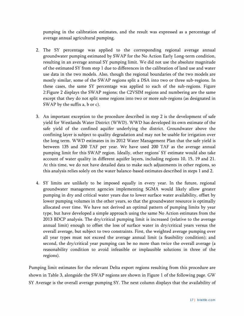
2. The SY percentage was applied to the corresponding regional average annual groundwater pumping estimated by SWAP for the No Action Early Long-term condition, resulting in an average annual SY pumping limit. We did not use the absolute magnitude of the estimated SY from step 1 due to differences in the calibration of land use and water use data in the two models. Also, though the regional boundaries of the two models are mostly similar, some of the SWAP regions split a DSA into two or three sub-regions. In these cases, the same SY percentage was applied to each of the sub-regions. Figure 2:Figure 2 displays the SWAP regions; the C2VSIM regions and numbering are the same except that they do not split some regions into two or more sub-regions (as designated in SWAP by the suffix a, b or c).

3. An important exception to the procedure described in step 2 is the development of safe yield for Westlands Water District (WWD). WWD has developed its own estimate of the safe yield of the confined aquifer underlying the district. Groundwater above the confining layer is subject to quality degradation and may not be usable for irrigation over the long term. WWD estimates in its 2012 Water Management Plan that the safe yield is between 135 and 200 TAF per year. We have used 200 TAF as the average annual pumping limit for this SWAP region. Ideally, other regions’ SY estimate would also take account of water quality in different aquifer layers, including regions 10, 15, 19 and 21. At this time, we do not have detailed data to make such adjustments in other regions, so this analysis relies solely on the water balance-based estimates described in steps 1 and 2.

4. SY limits are unlikely to be imposed equally in every year. In the future, regional groundwater management agencies implementing SGMA would likely allow greater pumping in dry and critical water years due to lower surface water availability, offset by lower pumping volumes in the other years, so that the groundwater resource is optimally allocated over time. We have not derived an optimal pattern of pumping limits by year type, but have developed a simple approach using the same No Action estimates from the 2013 BDCP analysis. The dry/critical pumping limit is increased (relative to the average annual limit) enough to offset the loss of surface water in dry/critical years versus the overall average, but subject to two constraints. First, the weighted average pumping over all year types must not exceed the average annual limit (a feasibility condition); and second, the dry/critical year pumping can be no more than twice the overall average (a reasonability condition to avoid infeasible or implausible solutions in three of the regions).

Pumping limit estimates for the relevant Delta export regions resulting from this procedure are

shown in Table 3, alongside the SWAP regions are shown in Figure 1 of the following page. GW

SY Average is the overall average pumping SY. The next column displays that the availability of

18 | brattle.com

groundwater based on average-year safe yields is projected to drop by more than 400,000 acre-

feet compared to the early long-term No Action analysis prepared in 2013. The final column is

the dry/critical year pumping limit.

It should be noted that the groundwater pumping restrictions assumed to be implemented as a

result of SGMA have a significant effect on the marginal value of surface water supplies received

by agriculture. This result makes economic sense: groundwater is a substitute for surface water,

and when groundwater usage is constrained, the value of surface water should increase. This

empirical result also suggests an important policy consideration, namely that by stabilizing

surface water deliveries to agriculture, the California WaterFix is complementary to the state’s

objective of sustainable groundwater management.

19 | brattle.com

Figure 2: SWAP Regions

Table 3: Estimated Safe Yield Groundwater Pumping Limits

(Thousand Acre-Feet)

Source: CH2M Hill.

SWAP Region

GW SY, Average

As Percentage of No Action Avg.

GW Pumped

GW SY, Dry/Critical

Years

10 285.2 0.97 424.914A 200 0.42 40014B 40 0.69 4015A 905.1 0.95 931.815B 30.9 0.95 40.119A 73.1 0.68 116.719B 199.6 0.68 254.920 173.5 0.49 212.221A 124.8 0.73 167.821B 38.4 0.73 76.821C 81 0.73 92.9

20 | brattle.com

VII. Water Quality Benefits

Construction of the California WaterFix will lower the salinity of water supplies exported from

the Delta via the SWP. These reductions in salinity benefit farmers and urban water users, and

this section describes the models used to value water quality improvements resulting from

construction of Stage I. The average salinity of SWP deliveries is 302 mg/l at present. The salinity

of SWP deliveries would be reduced to 221 mg/l as a result of Stage I of WaterFix.

The urban water quality benefits of Stage I of the WaterFix are calculated using two models. The

Lower Colorado River Basin Water Quality Model (LCRBWQM) assesses the cost to water users

for the MWD service area. The South Bay Water Quality model was used for the Bay Area urban

agencies. These models value reduced salinity according to improvements in taste and expended

appliance life, among other factors.

Reducing the salinity of SWP water supplies also provides benefit to agricultural customers. The

economic effects of changes in the quality of irrigation water are complex and may occur in the

short term and over the long term. Numerous water quality constituents may specifically affect

agricultural production, but salinity, measured as electrical conductivity or parts per million of

total dissolved solids, is the single best indicator of the overall quality of water delivered from the

Delta. Improved irrigation water quality means less water is applied to leach salts, and for

purposes of this analysis, that conserved water is valued as the avoided cost of additional water

supply, accounting for the different crops grown in affected delivery areas.

The long-term value of salinity changes resulting from implementing Stage I of the WaterFix

depends upon interactions between irrigation management, crop selection and groundwater

conditions. Poor drainage conditions in many areas receiving irrigation water from the Delta

indicate that costs of drainage management could be avoided or postponed by improved quality

of delivered water. Changes in surface water delivered also affects the use of groundwater for

irrigation, which can have up to or three times the total dissolved solids concentration as water

from the Delta. Longer-term implications of salt management in areas receiving Delta irrigation

water are not evaluated here. Therefore, the quantified salinity benefits presented in this report

should be viewed as a conservative estimate.

The salt leaching benefit provided by the improved quality of delivered water is calculated in

two components:

21 | brattle.com

• For the portion of project supply that replaces groundwater pumping, the benefit is calculated relative to the applied groundwater quality.

• For all other applied project water, the benefit is calculated relative to the baseline project water quality.

These two components affect how the overall irrigation water quality changes, especially in the

context of groundwater replacement of changes in surface water delivery.

VIII. Earthquake Reliability

By adding redundancy to the Delta’s water conveyance infrastructure, Stage I of the California

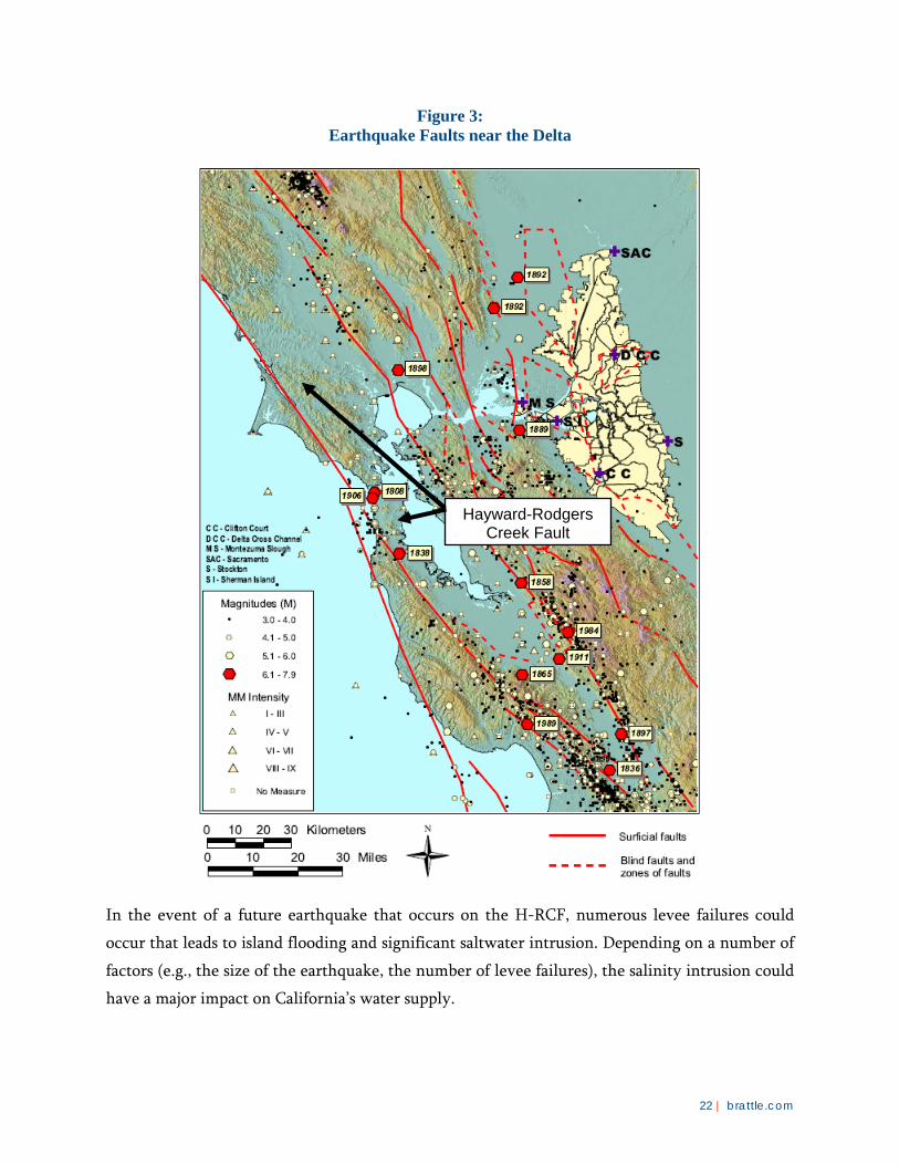
WaterFix addresses the seismic risks associated with the current Delta infrastructure. Figure 3 displays active faults and historic seismicity in the area surrounding the Delta. Of particular

interest is the Hayward-Rodgers Creek Fault (H-RCF). The H-RCF is located west of the Delta

and east of San Francisco Bay. Based on the USGS analysis of earthquake potential in the Bay

Area, the Hayward-Rodgers Creek Fault has the highest probability (27%) of a magnitude 6.7 or

greater event occurring in the next 30 years of all the major faults in the region. Estimates of the

maximum magnitude for the Hayward-Rodgers Creek Fault vary from 6.5 to 7.3. To demonstrate

the seismic risk reduction benefits of California WaterFix, this report considers the effects of a

magnitude 6.7 earthquake on the Hayward-Rodgers Creek Fault.

22 | brattle.com

Figure 3: Earthquake Faults near the Delta

In the event of a future earthquake that occurs on the H-RCF, numerous levee failures could

occur that leads to island flooding and significant saltwater intrusion. Depending on a number of

factors (e.g., the size of the earthquake, the number of levee failures), the salinity intrusion could

have a major impact on California’s water supply.

Hayward-Rodgers Creek Fault

23 | brattle.com

This section details the steps taken to simulate changes in Delta exports following a large

earthquake near the Delta. This section also describes the IRPSIM model developed by MWD

that was used to simulate changes in end use, storage and costs of operations for MWD and

several other SWP contracting water agencies. The section concludes with a description of

economic impacts using the impact framework detailed in the previous section.

The earthquake scenario considered in this report is evaluated using the tools developed as part

of the California Department of Water Resources Delta Risk Management Strategy (DRMS)

project Specifically, the DRMS Seismic Risk Analysis (SRA), Emergency Response and Repair

(ERR) and the Water Analysis Module (WAM) tools (software packages) are used to evaluate the

water supply impact of seismically initiated levee failures in the Delta.

Earthquake Scenario - The first step in the analysis is to define the earthquake scenario to be

evaluated. An earthquake scenario is defined for a specific seismic source (e.g., fault), a specified

earthquake size (magnitude) and a location. The size of the earthquake is typically selected as

the estimated maximum magnitude that can be generated by the fault. The earthquake location is

defined by the closest approach of the fault to the site or region of interest.

Seismic Risk Analysis (SRA) - Given the occurrence of an earthquake on a fault of a specific

magnitude (an earthquake scenario), the DRMS seismic risk analysis software evaluates the

earthquake ground motions that may be generated and the performance of the levees on each

island in the Delta. Empirical studies of earthquake ground motions demonstrate the ground

motions that can be generated are random, even for an event that occurs on a specific fault of

known magnitude. Similarly, the response of Delta levees to earthquake shaking cannot be

predicted exactly and as a result how many and which levees may fail during an earthquake is

also random. The DRMS seismic risk analysis code evaluates the randomness of ground motions

and levee performance and generates sequences of flooded islands. A sequence is a specific list of

which levees have failed and which islands are breached as a result of an earthquake. Since the

ground motions that can occur and the performance of the levees are random, there are many

possible combinations of flooded islands that can occur as a result of single earthquake. As a

result, the SRA calculates thousands of sequences (each representing a different combination of

flooded islands) that quantify the randomness in levee performance.

Emergency Response and Repair (ERR) - Following an earthquake that results in levee failures,

repairs are made to close levee breaches and damaged levee sections and to dewater flooded

islands. The ERR is a simulation code that models the repair of levees that were damaged or

24 | brattle.com

breached in a sequence. It takes into account the rate of quarry production, rock placement and

the potential for levee interior erosion that can occur on flooded islands (e.g., such as occurred

on Jones Tract in 2004). The ERR model produces a time series of breach closures and island

dewatering that serves as input to the WAM model. In addition, ERR estimates the cost of levee

repairs.

Water Analysis Module (WAM) - The Water Analysis Module simulates direct, water-quality-

related consequences of levee breach sequences. Specifically, WAM incorporates initial island

flooding, upstream reservoir management response, Delta water operations, water quality

(salinity) disruption of Delta irrigation, Delta net losses (or net consumptive water use),

hydrodynamics, water quality (initially represented by salinity) and water export. The module

receives the description of each breach scenario (e.g., resulting from a seismic or other event) and

details of the levee repair process from the ERR. The model produces hydrodynamic, water

quality and water supply consequences for use in the economic and ecosystem modules. The

water quality consequences of levee failures are dependent not only on the initial state of the

Delta at the time of failure, but also on the time series of tides, inflows, exports, other uses and on

the water management decisions that influence these factors. Thus, WAM tracks water

management and the Delta’s water quality response starting before the initial breach event and

proceeding through the breach, emergency operations, repair and recovery period.

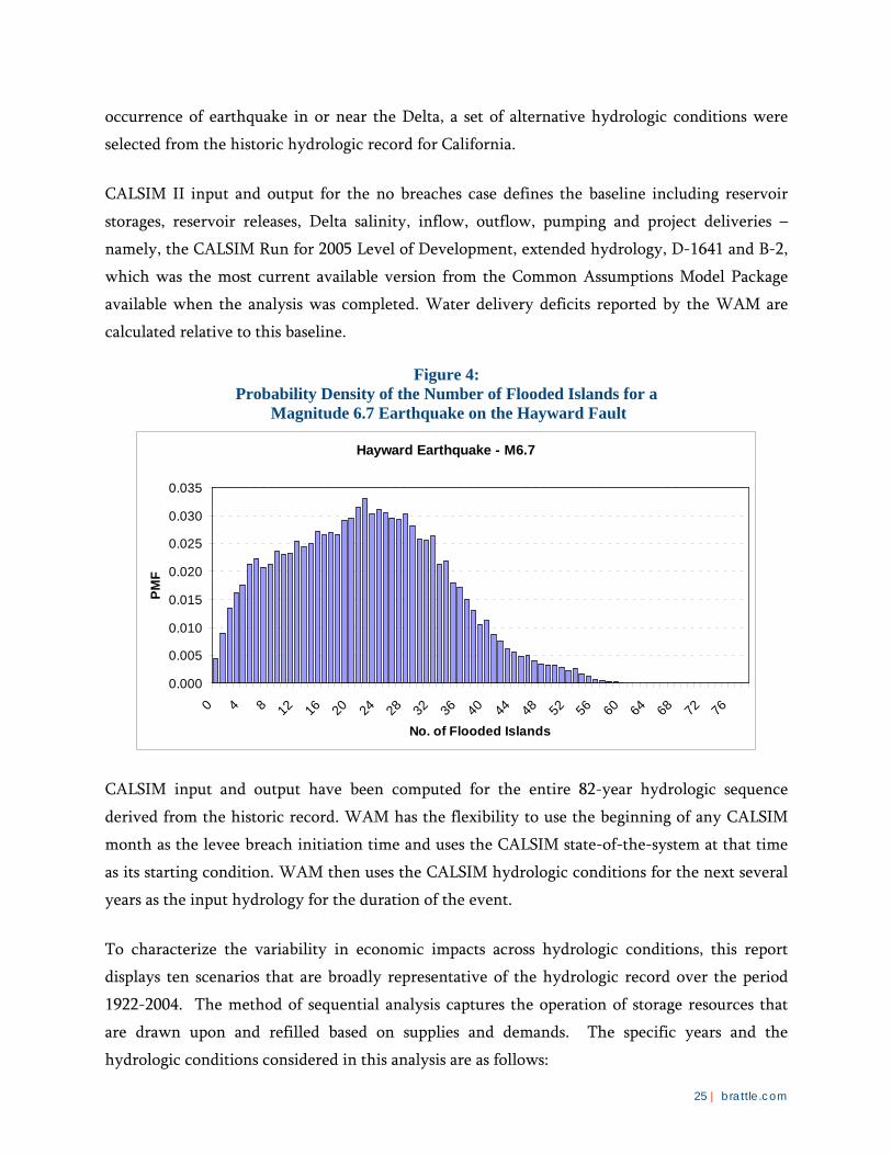
As described above, this report examines the consequences of a magnitude 6.7 earthquake on the

H-RCF. The DRMS study team generated thousands of levee failure sequences for each

earthquake simulated. Figure 4 shows the distribution of the number of flooded islands for the

6.7 earthquake scenario on the H-RCF. As seen in the figures, the randomness in ground motions

and levee performance provides a wide range in terms of the number of islands that are flooded

as a result of levee failures.

For purposes of estimating economic consequences, the mean number of flooded islands was

used. For the M 6.7 event, the mean number of flooded islands is 22. To estimate economic

impacts, a sequence with the mean number of islands was selected. These sequences were used in

the ERR and WAM calculations to estimate the water conveyance impacts.

The impact of levee failures to water conveyance in the Delta depends on the time of the year

the event (Start Time) occurs and the hydrologic conditions at the time. For instance, does the

event occur in the middle of a long drought or during a period of above normal precipitation and

snow? To model the impact of hydrologic conditions on water conveyance following the random

25 | brattle.com

occurrence of earthquake in or near the Delta, a set of alternative hydrologic conditions were

selected from the historic hydrologic record for California.

CALSIM II input and output for the no breaches case defines the baseline including reservoir

storages, reservoir releases, Delta salinity, inflow, outflow, pumping and project deliveries –

namely, the CALSIM Run for 2005 Level of Development, extended hydrology, D-1641 and B-2,

which was the most current available version from the Common Assumptions Model Package

available when the analysis was completed. Water delivery deficits reported by the WAM are

calculated relative to this baseline.

Figure 4: Probability Density of the Number of Flooded Islands for a

Magnitude 6.7 Earthquake on the Hayward Fault

CALSIM input and output have been computed for the entire 82-year hydrologic sequence

derived from the historic record. WAM has the flexibility to use the beginning of any CALSIM

month as the levee breach initiation time and uses the CALSIM state-of-the-system at that time

as its starting condition. WAM then uses the CALSIM hydrologic conditions for the next several

years as the input hydrology for the duration of the event.

To characterize the variability in economic impacts across hydrologic conditions, this report

displays ten scenarios that are broadly representative of the hydrologic record over the period

1922-2004. The method of sequential analysis captures the operation of storage resources that

are drawn upon and refilled based on supplies and demands. The specific years and the

hydrologic conditions considered in this analysis are as follows:

Hayward Earthquake - M6.7

0.000

0.005

0.010

0.015

0.020

0.025

0.030

0.035

0 4 8 12 16 20 24 28 32 36 40 44 48 52 56 60 64 68 72 76

No. of Flooded Islands

PMF

26 | brattle.com

• Wet year followed by 2 wet years -- 1969

• Wet year followed by 2 normal years -- 1971

• Wet year followed by 2 below normal or dry years-- 1958

• Normal year followed by 2 above normal or wet years -- 1972

• Normal year followed by 2 normal years -- 1936 (Note – There was no sequence in the historic record that matched this condition; 1938 is a wet rather than normal year)

• Normal year followed by 2 below normal or dry years -- 1946

• Dry year followed by 2 above normal or wet years -- 1939

• Dry year followed by 2 normal years -- 1949

• Dry year followed by 2 below normal or dry years -- 1947

• Dry followed by two dry or critical years -- 1987

There exists uncertainty about the exact number and location of failed levees, optimal repair

methods and times and daily natural inflow following a particular earthquake. All of these factors

result in uncertainty about the exact pattern of water supply outages. To model this uncertainty,

the DRMS post-earthquake water supply scenarios were modified as follows. The DRMS water

supply runs for the 10 hydrologies specified above list a unique recovery date after which the

post-earthquake and baseline water supplies converge. Water supplies may be available to some

degree prior to this recovery date, but not in all cases. The study team defined four partial outage

scenarios for this analysis. These partial delivery scenarios specify no Delta exports for some

fraction (25, 50, 75 and 100%) of the DRMS-specified recovery time. The average recovery time

across the 10 hydrologies was 30 months, meaning that the average cessation of Delta exports in

the 25% scenario is 7.5 months, 15 months for the 50% scenario, etc.

An additional dimension to the analysis is that we consider two scenarios for the allocation of

end-use shortages. In the first scenario, all losses are absorbed by the residential sector. While

this common approach preserves businesses and protects jobs, it can also lead to large economic

losses for residential consumers. For this reason, we also consider an optimal reduction scenario

where the residential, commercial, industrial and agricultural sectors are targeted to minimize

welfare loss.

Delta export losses are translated into changes in end-use with an augmented version of the

SDBSIM model that incorporates MWD wholesale agencies and several non-MWD urban

contractors. SDBSIM is based on MWD’s IRPSIM model and is implemented using a Monte Carlo

simulation approach that integrates projections of water demands and imported water supplies

27 | brattle.com

for each forecast year and adjusts each projection according to weather conditions based on

assumed hydrologies. For agencies within the MWD service area, the SDBSIM model integrates

retail urban water demand projections (MWD-EDM), local supply and imported water

projections (MWD Sales Model), SWP imported water supplies (CALSIM/DWRSIM) and

Colorado River Aqueduct (CRA) imported water supplies (CRSS) and results in a set of supply

and demand conditions over the 10 year period 2010-2019 that are indexed to various

hydrologies. For non-MWD agencies, similar information on demands, imported water and

storage is provided directly. 19 20

Water supply losses vary widely by hydrology, as does recovery time. It bears repeating that

these water supply losses are entirely caused by changes in the salinity that make it impossible to

export water during some months. Recovery times are defined as the number of months

following the earthquake necessary for baseline and post-earthquake water quality profiles to

converge.

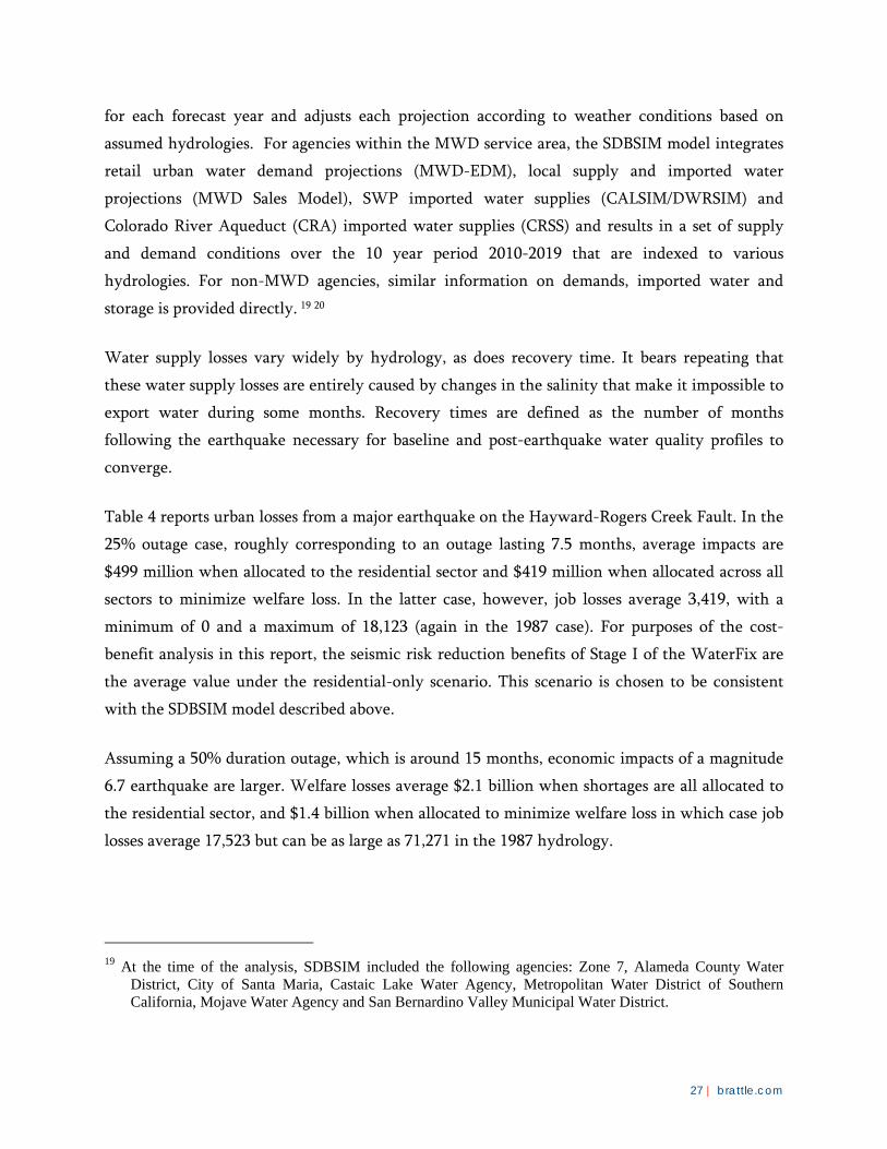
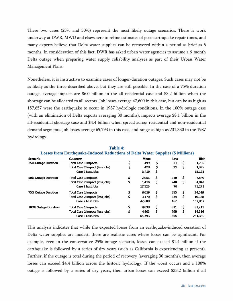
Table 4 reports urban losses from a major earthquake on the Hayward-Rogers Creek Fault. In the

25% outage case, roughly corresponding to an outage lasting 7.5 months, average impacts are

$499 million when allocated to the residential sector and $419 million when allocated across all

sectors to minimize welfare loss. In the latter case, however, job losses average 3,419, with a

minimum of 0 and a maximum of 18,123 (again in the 1987 case). For purposes of the cost-

benefit analysis in this report, the seismic risk reduction benefits of Stage I of the WaterFix are

the average value under the residential-only scenario. This scenario is chosen to be consistent

with the SDBSIM model described above.

Assuming a 50% duration outage, which is around 15 months, economic impacts of a magnitude

6.7 earthquake are larger. Welfare losses average $2.1 billion when shortages are all allocated to

the residential sector, and $1.4 billion when allocated to minimize welfare loss in which case job

losses average 17,523 but can be as large as 71,271 in the 1987 hydrology.

19 At the time of the analysis, SDBSIM included the following agencies: Zone 7, Alameda County Water

District, City of Santa Maria, Castaic Lake Water Agency, Metropolitan Water District of Southern California, Mojave Water Agency and San Bernardino Valley Municipal Water District.

28 | brattle.com

These two cases (25% and 50%) represent the most likely outage scenarios. There is work

underway at DWR, MWD and elsewhere to refine estimates of post-earthquake repair times, and

many experts believe that Delta water supplies can be recovered within a period as brief as 6

months. In consideration of this fact, DWR has asked urban water agencies to assume a 6-month

Delta outage when preparing water supply reliability analyses as part of their Urban Water

Management Plans.

Nonetheless, it is instructive to examine cases of longer-duration outages. Such cases may not be

as likely as the three described above, but they are still possible. In the case of a 75% duration

outage, average impacts are $6.0 billion in the all-residential case and $3.2 billion when the

shortage can be allocated to all sectors. Job losses average 47,600 in this case, but can be as high as

157,657 were the earthquake to occur in 1987 hydrologic conditions. In the 100% outage case

(with an elimination of Delta exports averaging 30 months), impacts average $8.1 billion in the

all-residential shortage case and $4.4 billion when spread across residential and non-residential

demand segments. Job losses average 65,793 in this case, and range as high as 231,330 in the 1987

hydrology.

Table 4: Losses from Earthquake-Induced Reductions of Delta Water Supplies ($ Millions)

This analysis indicates that while the expected losses from an earthquake-induced cessation of

Delta water supplies are modest, there are realistic cases where losses can be significant. For

example, even in the conservative 25% outage scenario, losses can exceed $1.4 billion if the

earthquake is followed by a series of dry years (such as California is experiencing at present).

Further, if the outage is total during the period of recovery (averaging 30 months), then average

losses can exceed $4.4 billion across the historic hydrology. If the worst occurs and a 100%

outage is followed by a series of dry years, then urban losses can exceed $33.2 billion if all

29 | brattle.com

mandatory conservation is placed on the residential sector. If this proves to be infeasible and

water shortages must be allocated across all sectors, then job losses increase to as much as

231,330. Thus, construction of Stage I of the WaterFix can prevent significant economic

dislocation in the event of a major earthquake that occurs under drought conditions.

IX. Climate Change Mitigation

The existing intakes of the State Water Project and Central Valley Project are just three feet

above mean sea level, making them highly vulnerable to the effects of sea level rise. The

proposed intakes on the Sacramento River in the northern Delta, in comparison, are about 14

feet above sea level.

Sea level rise poses a significant threat to the Delta’s water supply infrastructure. The current

intakes are close to sea level, and any rise in the ocean’s surface level means that the state and

federal pumps are inundated with salt water more frequently, resulting in a loss of project

deliveries. California WaterFix is expected to mitigate the impacts of sea level rise due to the

construction of a second set of intakes on the Sacramento River upstream of the Delta and at a

higher elevation than the current intakes. Indeed, the California WaterFix maintains SWP

deliveries through the Delta at roughly their current levels. Without north Delta intakes, yields

fall significantly. This result makes adaptation to climate change one of the strongest arguments

in favor of California WaterFix, although it is a difficult one to quantify with certainty.

Recent modeling suggests the climate mitigation benefits from Stage I of the California WaterFix

may be substantial. With 140 cm of sea level rise, now considered to be a middle of the road

scenario, Delta deliveries to urban and agricultural customers via the SWP may fall by roughly

half relative to their current levels. This report does not monetize the value of these climate

change mitigation benefits of the California WaterFix. There is substantial uncertainty about

how climate change will evolve over the coming decades, and the results presented here should

be considered as illustrative of potential outcomes. Second, there is uncertainty about the exact

timing of climate impacts. While the model results correspond to 2100 levels of development, sea

level rise may occur more rapidly or slowly than expected. Nonetheless, the water supply results

for 140-cm of sea level rise should be of concern to water district managers and policy makers,

and indicate that California WaterFix can be an important part of California’s overall strategy to

mitigate the effects of climate change on the state’s economy.

30 | brattle.com

X. Quantified Benefits and Costs to Participating Agencies

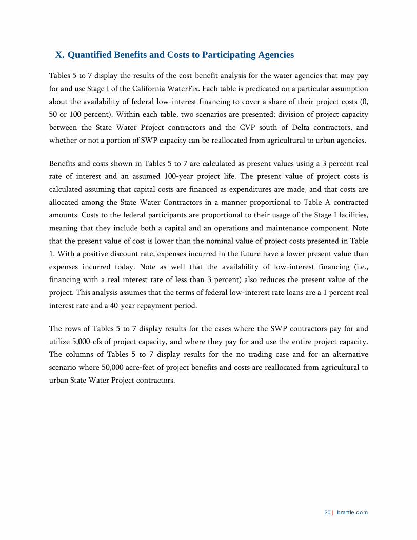
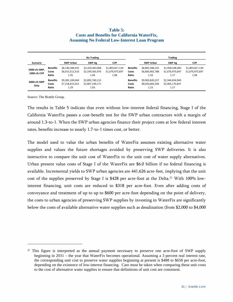
Tables 5 to 7 display the results of the cost-benefit analysis for the water agencies that may pay

for and use Stage I of the California WaterFix. Each table is predicated on a particular assumption

about the availability of federal low-interest financing to cover a share of their project costs (0,

50 or 100 percent). Within each table, two scenarios are presented: division of project capacity

between the State Water Project contractors and the CVP south of Delta contractors, and

whether or not a portion of SWP capacity can be reallocated from agricultural to urban agencies.

Benefits and costs shown in Tables 5 to 7 are calculated as present values using a 3 percent real

rate of interest and an assumed 100-year project life. The present value of project costs is

calculated assuming that capital costs are financed as expenditures are made, and that costs are

allocated among the State Water Contractors in a manner proportional to Table A contracted

amounts. Costs to the federal participants are proportional to their usage of the Stage I facilities,

meaning that they include both a capital and an operations and maintenance component. Note

that the present value of cost is lower than the nominal value of project costs presented in Table

1. With a positive discount rate, expenses incurred in the future have a lower present value than

expenses incurred today. Note as well that the availability of low-interest financing (i.e.,

financing with a real interest rate of less than 3 percent) also reduces the present value of the

project. This analysis assumes that the terms of federal low-interest rate loans are a 1 percent real

interest rate and a 40-year repayment period.

The rows of Tables 5 to 7 display results for the cases where the SWP contractors pay for and

utilize 5,000-cfs of project capacity, and where they pay for and use the entire project capacity.

The columns of Tables 5 to 7 display results for the no trading case and for an alternative

scenario where 50,000 acre-feet of project benefits and costs are reallocated from agricultural to

urban State Water Project contractors.

31 | brattle.com

Table 5: Costs and Benefits for California WaterFix,

Assuming No Federal Low-Interest Loan Program

Source: The Brattle Group.

The results in Table 5 indicate that even without low-interest federal financing, Stage I of the

California WaterFix passes a cost-benefit test for the SWP urban contractors with a margin of

around 1.3-to-1. When the SWP urban agencies finance their project costs at low federal interest

rates, benefits increase to nearly 1.7-to-1 times cost, or better.

The model used to value the urban benefits of WaterFix assumes existing alternative water

supplies and values the future shortages avoided by preserving SWP deliveries. It is also

instructive to compare the unit cost of WaterFix to the unit cost of water supply alternatives.

Urban present value costs of Stage I of the WaterFix are $6.0 billion if no federal financing is

available. Incremental yields to SWP urban agencies are 441,626 acre-feet, implying that the unit

cost of the supplies preserved by Stage I is $428 per acre-foot at the Delta.21 With 100% low-

interest financing, unit costs are reduced to $318 per acre-foot. Even after adding costs of

conveyance and treatment of up to up to $600 per acre-foot depending on the point of delivery,

the costs to urban agencies of preserving SWP supplies by investing in WaterFix are significantly

below the costs of available alternative water supplies such as desalination (from $2,000 to $4,000

21 This figure is interpreted as the annual payment necessary to preserve one acre-foot of SWP supply

beginning in 2031 – the year that WaterFix becomes operational. Assuming a 3 percent real interest rate, the corresponding unit cost to preserve water supplies beginning at present is $488 to $658 per acre-foot, depending on the existence of low-interest financing. Care must be taken when comparing these unit costs to the cost of alternative water supplies to ensure that definitions of unit cost are consistent.

Scenario SWP Urban SWP Ag CVP SWP Urban SWP Ag CVP

Benefits $8,140,289,432 $2,429,463,066 $1,803,817,134 Benefits $8,892,586,225 $1,958,548,483 $1,803,817,134Costs $6,015,512,510 $2,339,365,976 $1,670,975,697 Costs $6,683,902,788 $1,670,975,697 $1,670,975,697Ratio 1.35 1.04 1.08 Ratio 1.33 1.17 1.08

Benefits $9,281,100,044 $2,892,740,115 Benefits $9,903,820,227 $2,344,654,949Costs $7,218,615,012 $2,807,239,171 Costs $8,020,683,346 $2,005,170,837Ratio 1.29 1.03 Ratio 1.23 1.17

5000-cfs SWP, 1000-cfs CVP

6000-cfs SWP Only

No Trading Trading

32 | brattle.com

per acre-foot) or recycling (highly site-specific, but often around $1,500 - $2,500 per acre-foot

and not available for direct potable use).22

Stage I of the California WaterFix also passes a benefit cost test for SWP agriculture, although by

a smaller margin than is for the SWP urban agencies. In the least-favorable case where the

project is financed at market interest rates and no trading is allowed, the net benefits of Stage I to

SWP agricultural contractors are small but positive. With low-interest financing and an ability to

trade project shares, however, the picture for SWP agriculture improves significantly. When 100

percent of project costs are financed at low interest rates and SWP contractors can trade project

shares, for example, the benefit-cost ratio for the SWP agricultural contractors improves to

nearly 1.6-to-1.

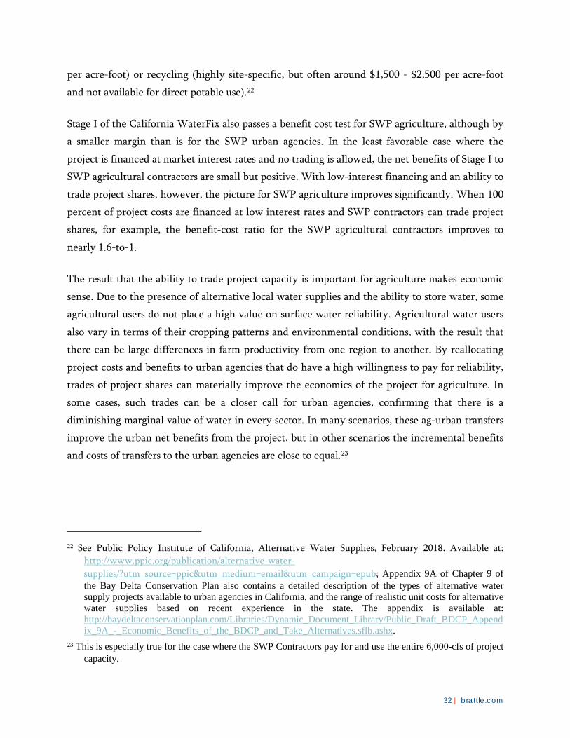
The result that the ability to trade project capacity is important for agriculture makes economic

sense. Due to the presence of alternative local water supplies and the ability to store water, some

agricultural users do not place a high value on surface water reliability. Agricultural water users

also vary in terms of their cropping patterns and environmental conditions, with the result that

there can be large differences in farm productivity from one region to another. By reallocating

project costs and benefits to urban agencies that do have a high willingness to pay for reliability,

trades of project shares can materially improve the economics of the project for agriculture. In

some cases, such trades can be a closer call for urban agencies, confirming that there is a

diminishing marginal value of water in every sector. In many scenarios, these ag-urban transfers

improve the urban net benefits from the project, but in other scenarios the incremental benefits

and costs of transfers to the urban agencies are close to equal.23

22 See Public Policy Institute of California, Alternative Water Supplies, February 2018. Available at:

http://www.ppic.org/publication/alternative-water-supplies/?utm_source=ppic&utm_medium=email&utm_campaign=epub; Appendix 9A of Chapter 9 of the Bay Delta Conservation Plan also contains a detailed description of the types of alternative water supply projects available to urban agencies in California, and the range of realistic unit costs for alternative water supplies based on recent experience in the state. The appendix is available at: http://baydeltaconservationplan.com/Libraries/Dynamic_Document_Library/Public_Draft_BDCP_Appendix_9A_-_Economic_Benefits_of_the_BDCP_and_Take_Alternatives.sflb.ashx.

23 This is especially true for the case where the SWP Contractors pay for and use the entire 6,000-cfs of project capacity.

http://www.ppic.org/publication/alternative-water-supplies/?utm_source=ppic&utm_medium=email&utm_campaign=epub

http://www.ppic.org/publication/alternative-water-supplies/?utm_source=ppic&utm_medium=email&utm_campaign=epub

http://baydeltaconservationplan.com/Libraries/Dynamic_Document_Library/Public_Draft_BDCP_Appendix_9A_-_Economic_Benefits_of_the_BDCP_and_Take_Alternatives.sflb.ashx

http://baydeltaconservationplan.com/Libraries/Dynamic_Document_Library/Public_Draft_BDCP_Appendix_9A_-_Economic_Benefits_of_the_BDCP_and_Take_Alternatives.sflb.ashx

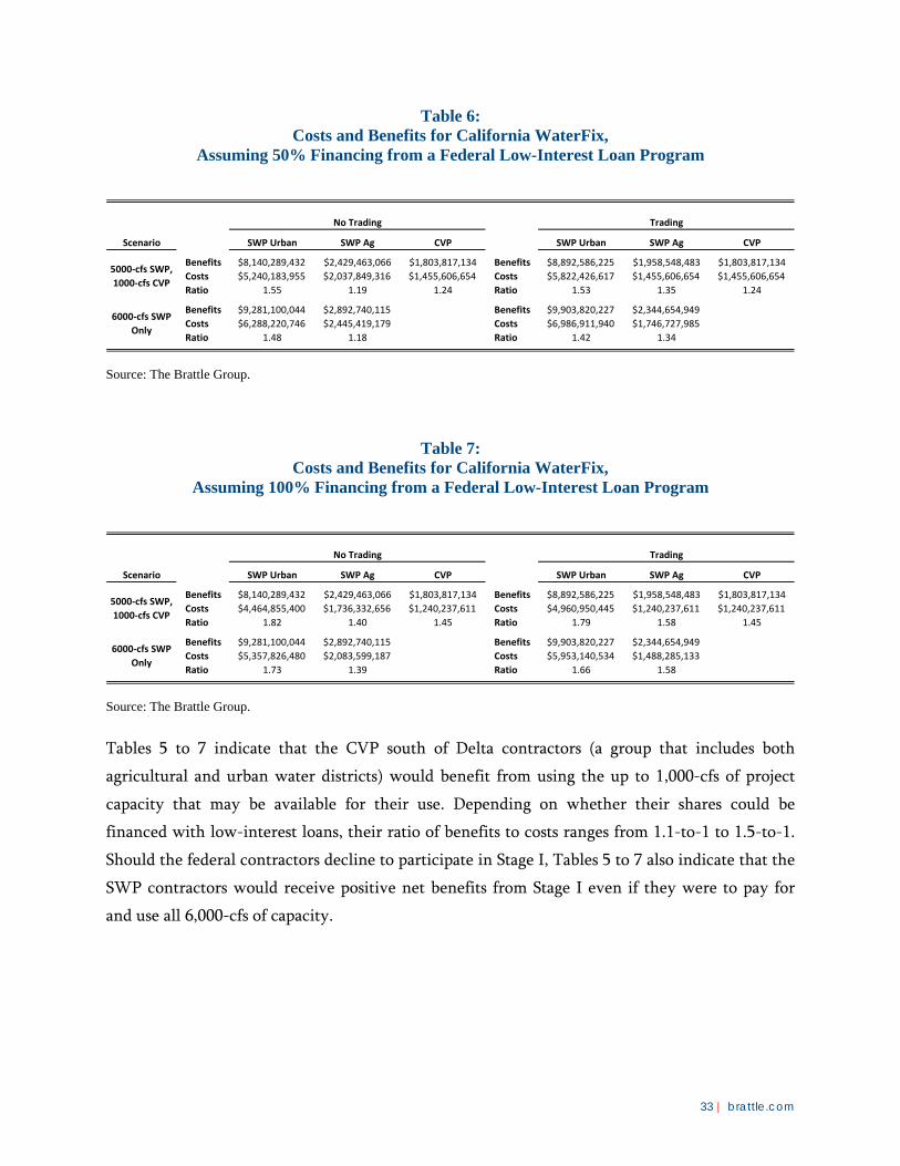
33 | brattle.com


Assuming 50% Financing from a Federal Low-Interest Loan Program



Assuming 100% Financing from a Federal Low-Interest Loan Program


Tables 5 to 7 indicate that the CVP south of Delta contractors (a group that includes both

agricultural and urban water districts) would benefit from using the up to 1,000-cfs of project

capacity that may be available for their use. Depending on whether their shares could be

financed with low-interest loans, their ratio of benefits to costs ranges from 1.1-to-1 to 1.5-to-1.

Should the federal contractors decline to participate in Stage I, Tables 5 to 7 also indicate that the

SWP contractors would receive positive net benefits from Stage I even if they were to pay for

and use all 6,000-cfs of capacity.





6000-cfs SWP Only

No Trading Trading





6000-cfs SWP Only

No Trading Trading

34 | brattle.com