Oil PrCountrMamotUniversiReneé UniversiRanganUniversiMark EUniversiWorkingFebruary _______DepartmUnivers0002, PrSouth ATel: +27

rice Volatries using thoana Difity of Pretorvan Eydenity of Pretorn Gupta ity of Pretor

E. Wohar ity of Nebrag Paper: 201y 2018

__________ment of Econsity of Pretoretoria

Africa 7 12 420 24

Depart

tility and over One

feto ria n ria

ria

aska at Omah18-13

__________nomics ria

13

Univtment of Ec

Economie Century

ha and Loug

__________

versity of Prconomics W

ic Growthof Data

ghborough U

__________

retoria Working Pap

h: Eviden

University

__________

per Series

nce from A

_______

Advancedd OECD

1

Oil Price Volatility and Economic Growth: Evidence from Advanced OECD Countries

using over One Century of Data

Mamothoana Difeto, Reneé van Eyden, Rangan Gupta and Mark E. Wohar*

Abstract

In this paper we make use of a number of different panel data estimators, including fixed effects, bias-

corrected least squares dummy variables (LSDVC), generalised methods of moments (GMM), feasible

generalised least squares (FGLS), and random coefficients (RC) to analyse the impact of real oil price

volatility on the growth in real GDP per capita for 17 member countries of the Organisation for Economic

Co-operation and Development (OECD), over a 144-year time period from 1870 to 2013. Our main

findings can be summarised as follows: overall, oil price volatility has a negative and statistically

significant impact on economic growth of OECD countries in our sample. In addition, when allowing for

slope heterogeneity, oil producing countries are significantly negatively impacted by oil price uncertainty,

most notably Norway and Canada.

Keywords: Oil price volatility, economic growth, OECD countries, panel data.

JEL Classification: Q43, C33, O55

Department of Economics, University of Pretoria, Pretoria, 0002, South Africa. Email: mamothoana@gmail.com. Corresponding author. Department of Economics, University of Pretoria, Pretoria, 0002, South Africa. Email: renee.vaneyden@up.ac.za. Department of Economics, University of Pretoria, Pretoria, 0002, South Africa. Email: rangan.gupta@up.ac.za. * College of Business Administration, University of Nebraska at Omaha, 6708 Pine Street, Omaha, NE 68182, USA; School of Business and Economics, Loughborough University, Leicestershire, LE11 3TU, UK. Email: mwohar@unomaha.edu.

2

1. Introduction

Given the importance of crude oil in the global economy, the impact of oil price volatility on economic

activity has received considerable attention after the 1973 and 1979 oil price shocks, following the Yom

Kippur war and the Iranian Revolution, respectively. Oil prices, like many other commodity prices, have

been volatile and characterised by uncertainties (Mehrara and Oskoui, 2007; El Anshashy and Bradley,

2012). According to Plourder and Watkins (1998), oil price swings have been larger than those of other

mineral resources during the period from 1985 to 1994. In September 1960, the Organization of the

Petroleum Exporting Countries (OPEC) was formed in Baghdad by its first five members. The mission of

OPEC is to coordinate and unify the petroleum policies of its member countries and ensure the

stabilisation of oil markets in order to secure an efficient, economic and regular supply of petroleum to

consumers, a steady income to producers and a fair return on capital for those investing in the petroleum

industry (OPEC, n.d.).

Theoretically, an increase in the oil price in oil exporting countries may be seen as a positive development

as it will increase revenue while increasing oil prices in oil importing countries could have an adverse

effect on economic activity. Given extensive use of oil as an input in the production process, it is

generally perceived that an increase in oil price volatility exerts substantial influence globally

(Swanepoel, 2006). The (adverse) effect of oil price uncertainty on aggregate economic activity is

generally explained by the theory of irreversible investment under uncertainty, following Henry (1974)

and Bernanke (1983). According to this theory, irreversible investments are postponed during the periods

of uncertainty which, in turn, causes temporary declines in aggregate output level. Hamilton (2003),

points out that the same also holds true for consumer, in terms of postponement of expenditures in the

wake of increased oil market volatility. Thus, the volatility in oil price creates uncertainty about the future

path of the oil price, resulting in consumers and firms to postpone investments, potentially requiring

expensive reallocation of resources.

Although a number of studies suggest that oil price increases have adverse effects on a country’s

macroeconomic growth prospects by increasing inflation and unemployment, and decreasing the value of

financial assets in oil importing countries (Awerbuch and Sauter, 2003), this claim has received mixed

empirical support. Hooker (1996) found no relationship between oil prices and macroeconomic variables.

On the other hand, Mork (1989), Mory (1993), Mork et al. (1994); Ferderer (1996); Brown and Yücel

(2002), Lardic and Mignon (2006, 2008) just to name a few, have proven a non-linear and asymmetric

relationship between oil price and economic activity. In particular, an increase in oil price may adversely

affect economic activity, but a fall in oil price may not necessarily increase the output level. So, if a fall in

3

oil price increases uncertainty about changes in the oil price, then a part of the increased output will be

offset by lowering of the output level due to increased uncertainty. Therefore, it might be that oil price

volatility (or uncertainty) in the oil price, rather than the level of the oil price, that is linked to the

aggregate level of output. Given that the world oil price has been volatile in general, one should ideally

include volatility and uncertain oil price behaviour in any econometric model that attempts to explain the

role of oil price changes in the macroeconomy.

Of course, the weak or the insignificant oil-price-growth relationship over the years may be attributed to

various factors including, a growing use of alternative energy sources such as renewable energy; efficient

use of oil, increase in utilisation of alternative energy sources and a shift in the composition of output

towards less oil intensive sectors. According to Iwayemi and Fowowe (2011), the results may differ from

one country to another, depending on countries’ level of development.

Most economists argue that that there was no world crude oil price before World War II. From 1948

through to the end of the 1960s, crude oil prices ranged between $2.50 and $3.00 per barrel. Historical

data indicate that prior to the 1970s; the price of oil remained relatively stable, however, the world

demand for oil has decreased drastically over the past 3 decades due to various reasons including a

reduced reliance on oil in production processes. Oil prices rose from 2004 to historic highs of $147 per

barrel in mid-2008 following the global financial crisis. Oil became the dominant fuel in the 20th century

and a primary part of the American economy. During 2014 to 2015 period, OPEC members consistently

exceeded their production ceiling, causing a collapse in oil prices that continued into early 2016.

Although there are several studies that pay attention to member countries of the Organisation for

Economic Co-operation and Development (OECD), these studies were mainly focused on the relationship

between either oil price shocks or oil price movements and the level of economic activity (e.g. Cuñado

and Pérez de Gracia, 2003; Jiménez-Rodríguez and Sánchez, 2005; and Jiménez-Rodríguez, 2008).

Moreover, the mainstream literature on oil price volatility does not typically go beyond single country,

time-series techniques. This paper differs in that it investigates the impact of oil market uncertainty in a

panel framework using over one century of data for advanced economies, and hence, takes a historical

perspective.

This paper aims to analyse the effects of oil price volatility on the growth rate of real GDP per capita of

the seventeen main industrialised OECD countries. While most of the countries included are net oil

importers, we also include in our sample net oil exporting countries, namely Norway, Canada and

Denmark. The UK, USA and Australia, even though net oil importing countries, are also large oil

producers, while Germany, France, Italy, Spain, the Netherlands and Japan have some domestic

4

production of oil to supplement imports. Hence, countries that are net importers of oil, but also large

producers of oil are included in our dataset spanning the annual period of 1870 to 2013, i.e., 144 years.

Methodologically, we measure uncertainty with respect to real oil prices using a realised oil price

variance series constructed from monthly crude oil prices. A selection of econometric techniques are

employed in this analysis including fixed effects (FE), Bruno’s (2005) bias-corrected least squares

dummy variables (LSDVC), Arellano-Bond (1991) generalised method of moments (GMM), feasible

generalised least squares (FGLS) and Swamy’s (1970) random coefficients (RC) estimator.

Our main findings may be summarized as follows: First, it is hypothesised that oil price volatility has a

negative and significant impact on economic growth of OECD countries in our sample. When allowing

for slope heterogeneity, oil prices volatility is found to have a negative impact on the real GDP growth of

all countries, with the exception of Portugal, where a positive, yet insignificant relationship is found. In

addition, the negative effects of oil price volatility on GDP growth are overall strongest for Norway and

Canada, while the UK, USA, Sweden, France, Finland and Japan exhibit similarly strong real effects.

Second, the paper finds that the extent to which economic growth is affected by oil price volatility varies

significantly across the different types of countries for example, the estimated sensitivity measure for

Norway is approximately double that of the USA.

The rest of the paper is structured as follows: the next section contains the literature review and

theoretical background of the role of oil price volatility in the economic growth process. Section 3

provides a discussion of the methodology used, followed by a description of the data employed in section

4. The estimation results are presented and discussed in section 5, while section 6 concludes.

2. Literature review

There has been a vast literature that examines the impact of oil price on economic activity since the early

pioneering work of Hamilton (1983). In his ground-breaking work, Hamilton (1983, 1985) finds that

since World War II, oil price shocks have preceded seven of eight US recessions the period 1948 1980

in the US economy. A detailed literature review of the impact of oil prices on international economies

(developed and developing) can be found in the recent work of Gupta et al., (forthcoming). Studies show

that increases in oil prices negatively affect macroeconomic activities of both oil-importing and oil-

exporting countries through both supply-side and demand-side channels, involving trade, unemployment,

investment, interest rates and inflation.

5

While a substantial number of empirical studies have concentrated on the link between oil price level

changes/shocks and economic activity, the literature that investigates the linkage between oil price

volatility (often associated with the standard deviation in a given period) and macroeconomic

performance is also quite vast. Empirically, numerous authors have found that increased oil price

uncertainty is associated with weaker macroeconomic activity. Early studies by Ferderer (1996), Sadorsky

(1999), and Guo and Kliesen (2005) found that oil price volatility has a negative and significant effect on

growth in gross domestic product. Bilgin et al. (2015), using data from 10 developing Asian countries

using a panel estimation technique, find that world energy volatility has a negative impact on aggregate

economic activity.

Elder and Serletis (2010) investigate the impact of oil price uncertainty on investment in the USA using a

multivariate GARCH in-mean VAR model and find that in developing countries, fluctuation in oil prices

tends to depress certain components of aggregate investment. In addition, Yoon and Ratti (2011) show

that increased energy price uncertainty makes US manufacturing firms cautious by reducing the

responsiveness of investment spending to sales growth. It is thus apparent that an increase in oil price

uncertainty may have an adverse effect on the economy through the demand channel, as the theory of

irreversible investments suggests. Elder and Serletis (2009, 2011), Bredin et al. (2011), Rahman and

Serletis (2011, 2012), and Bashar et al., (2013) also draws similar conclusions for other G7 countries.

Besides this, Rahman and Serletis (2010) have used a smooth transition vector autoregressive model to

show that an oil price shock reduces the output growth in the USA more in a high oil price volatility

regime than a low volatility regime. At the same time however, Hooker (1996) recognises that the effects

of oil price fluctuations on the US economy in the period following the 1973 oil shock were relatively

small and insignificant. Another interesting observation of a weakened relationship between oil price

volatility and economic activities arise in the studies by Blanchard and Gali (2010), and Nakov and

Pescatori (2010). The authors attribute this weakening relationship to various reasons including a better

monetary policy and reduced reliance on oil in production processes. While Bjørnland et al.,

(forthcoming) does not support this line of reasoning in terms of declining importance of oil volatility

shocks, they do tend to suggest that a change to a more responsive monetary policy regime by the US

Federal Reserve played a role.

Turning to developing markets, Egwaikhide and Omojolaibi (2013) employed a panel vector

autoregressive technique to examine the impact of oil price volatility on economic performance of five

oil-exporting countries in Africa and they conclude that gross investment is the main channel through

which volatility in oil price influenced the real sector of these economies. Aye, et al. (2015) investigate

the effect of oil price uncertainty on South African manufacturing production using monthly observations

6

covering the period 1974:02 to 2012:12. The authors quantify responses of manufacturing production to

positive and negative shocks. They make use of a bivariate GARCH-in-mean VAR simultaneously

estimated with full information maximum likelihood technique. Their results show that oil price

uncertainty negatively and significantly impacts on South Africa’s manufacturing production.

Furthermore, responses of manufacturing production to positive and negative shocks are asymmetric.

Using the same methodology, similar findings were derived for Jordan and Turkey by Maghyereh et al.

(2017). However, Jawad and Khan Niazi (2017) could not find any statistically significant impact of oil

price volatility (as measured by its standard deviation) using a VAR model for Pakistan, even though the

sign of the effect for the oil importing country was indeed negative.

In contrast, Akinlo and Apanisile (2015) estimated a panel data model for a sample of 20 sub-Saharan

African countries from the period of 1986 – 2012, showing that fluctuations in oil price has a positive and

insignificant impact on economic growth for non-oil producing countries but a positive and significant

effect for oil exporting countries. Using a dynamic stochastic general equilibrium (DSGE), Plante and

Traum (2012) confirmed the existence of this relationship with the finding that an increase in oil price

volatility is likely to result in an increase in investments and rise in real GDP due to heightened

precautionary savings motives.

De V. Cavalcanti et al. (2015) use panel data from 118 countries for the period 1970 to 2007 to study the

impact of volatility of commodity terms of trade on economic growth, total factor productivity, physical

capital accumulation, and human capital acquisition. They employed a standard system GMM approach

as well as the dynamic common correlated effects pooled mean group (CCEPMG) methodology for

estimation and they established that commodity terms of trade volatility exerts a negative impact on

economic growth.

In general, the impact of oil price volatility, barring certain cases, does tend to have a negative impact on

growth, based on post-World War II data across developed and developing countries, as well as, oil

exporters and importers. Our objective is to revisit this issue from a historical perspective by looking at

over one century of data of a panel of seventeen advanced economies, which includes both oil exporting

and importing economies. In the process, we deviate from usual country-based time series analysis and

provide a more comprehensive study of the impact of oil market volatility.

7

3. Methodology

3.1 Oil price volatility

The measurement of real oil price volatility is a highly contentious matter. Most empirical studies have

used either standard deviation of the moving average of the logarithm of the real oil price or the GARCH

model. In this paper, we employ the realised volatility (RV) method which was initially employed by

Andersen (2003) to measure volatility in the world energy price. The methodology expresses a price

process as a stochastic differential equation:

dlog ( ) = dt + (1)

where corresponds to a predictable drift term with a finite variance, denotes volatility, represents

a standard Brownian motion ,which is the continuously compounded price change in the unit interval

denoted as:

≡ log log (2)

where t1 . Then, based on the assumption that and are uncorrelated, the mean and

variance are calculated. In a standard Brownian motion, the increments are distributed according to

~ 0, for 0 , therefore the mean and the variance of are conditional on

information set and is written:

Ε | ≡ (3)

Var | ≡ = (4)

where is the integrated volatility.

In practice, the computation of return and volatility are restricted to discrete time intervals, therefore the

integrated volatility is underlying and can only be approximated. The volatility of daily changes can be

estimated by a monthly realized volatility series. The latter is a summation of squared daily changes in a

month over the period starting from the first to the final day of that month. The RV is given by the

following equation

=∑ =∑ (5)

8

where corresponds to the realised volatility of daily changes in a month. Andersen et al.

(2004) show that a h-period volatility is an unbiased and efficient estimator of since

converges uniformly in probability to as →0.

Therefore, for the annual frequency used in this study, the realized volatility is given by:

∑ (6)

where r is the log-returns of real oil price.1

3.2 The econometric model

The aim of this paper is to investigate the impact of oil price volatility on economic growth in OECD

countries. The model underling the empirical analysis closely follows the Barro (1998) specification

which is fairly popular in the literature. In this study, real oil price volatility is the key variable of interest.

To investigate the relationship, this we apply a number of panel data econometric techniques to estimate

variants of the following equation:

,

(7)

where gr is the dependent variable and defined as the growth in real GDP. A lagged dependent variable

has been included among the regressors to capture the dynamic nature of the economic growth process.

The primary variable of interest, roilunc, the annualised real oil price volatility is approximated by

realised volatility. signifies the inflation rate, while the investment to GDP ratio, expressed in natural

log terms, is denoted by . is defined as the log of government expenditure as a ratio to GDP,

while denotes log of public debt as a ratio to GDP. Real stock returns is denoted by .

is a dummy capturing systemic financial crises. The time span of the variables selected stretches

from 1870 to 2013.

Given that the study makes use of a dynamic growth model specification, and to deal with different types

of econometric issues and ensure robust results, we apply different estimators to the data set. As vantage

point, we apply cross-section fixed effects (FE) with robust standard errors. We employ Bruno’s (2005)

bias-corrected least square dummy variable (LSDV) method to correct for the Nickell (1981) bias. We

1 When we used monthly nominal returns or a GARCH(1,1) (as suggested by Sadorsky, 1999) based model of monthly conditional volatilities (for both real and nominal) oil returns to compute alternative measures of the annual realized volatilities, our results continued to be qualitatively and quantitatively similar to those reported in the paper. These analyses are available upon request from the authors.

9

also apply two-step differenced generalised methods of moments (GMM) with orthogonal deviations

(Arellano and Bover, 1995) to transform data to correct for endogeneity and eliminate dynamic panel

bias. Given the long time span of the data, we expect the bias to be marginal and results for these three

estimators should therefore be fairly robust (Judson and Owen, 1999). In addition, Swamy’s (1970)

random coefficients (RC) estimator and feasible generalised least squares (FGLS) are used to control for

slope heterogeneity and cross-sectional dependence.

The basic problem of including a lagged dependent variable as an explanatory variable is that the lagged

term becomes correlated with the unobserved individual effects in the error term leading to the Within

estimators being biased and inconsistent (Baltagi, 2013). Nickell (1981) demonstrates that even though

the Within transformation will wipe out the individual effects, the transformed lagged dependent variable

will still be correlated with the transformed error term. He also shows that the estimator is biased of order

O (1/T). To correct for this bias, Kieviet (1995) suggests employing the least squares dummy variable

(LSDV) estimator and then correcting the results for the bias. He derives a formula for the bias by using

asymptotic expansion techniques. Bruno (2005) extends the latter technique to unbalanced panels.

We employ the two-step difference generalised methods of moments (DIF-GMM) model to address the

dynamic nature of economic growth as well as the problems of endogeneity. Anderson and Hsiao (1981)

propose first-differencing (FD) the data to get rid of and then using Δyi,t-2 as an instrument for Δyi,t-1.

The instrumental variable estimation methods offer consistent but not necessarily efficient estimates

because it does not make use of all available moment conditions and it does not take into account the

differenced structure on the residual disturbances. Arellano and Bond (1991) consequently proposed a

more efficient estimation procedure, a generalised method of moments (GMM) procedure. They argue

that additional instruments can be obtained in a dynamic panel data model if one utilises the orthogonality

conditions that exist between lagged values of yit and the disturbance term vit. This transformation consists

of first-differencing the model to get rid of the individual effects and use all the past information of yit as

instruments. This is commonly referred to as the difference GMM (DIF-GMM). The two-step DIF-GMM

estimator is employed in this study to account for variance-covariance of the differenced error terms. In

two-step estimation, the standard covariance matrix is robust to panel-specific autocorrelation and

heteroscedasticity. Testing for first and second order serial correlation is important as the presence of

autocorrelation may suggest that certain variables may not be good instruments. Given that the model is

differenced, one expects to reject the null hypothesis of no first order serial correlation and fail to reject

the null hypothesis of no second order serial correlation (Baltagi, 2013).

10

As mentioned above, due to the lagged dependent variable in the model as an explanatory variable, a

certain degree of endogeneity is expected and this would render the fixed effects model more suitable

than the random effects estimator. The Hausman (1978) test is applied to both the dynamic and static

versions of the model to test for misspecification and to test whether endogeneity exists even when the

lagged dependent variable is excluded from the model. Given the inclusion of control variables such

inflation and public expenditure and debt, the expectation would be that a degree of economic endogenety

would be present in the relationship.

Fixed effect models control for group heterogeneity through the inclusion of a country-specific intercept

term. We may however improve on this by allowing for slope heterogeneity as well, i.e. allowing for the

fact that each country’s growth path is not necessarily affected by the same variables in exactly the same

way. Furthermore, the error terms of different cross sections may be correlated (cross-sectional

dependence). Not controlling for this heteroscedasticity will yield consistent estimates, but the estimates

will not be efficient. In this study we implement feasible generalised least squares (FGLS) with cross-

section weights, which controls for group heterogeneity and accounts for various patterns of correlation

between the residual (Parks, 1967). We also apply Swamy’s (1970) random coefficients (RC) regression

model. RC models are more general in that they allow each panel to have its own vector of slopes

randomly drawn from a distribution common to all panels. Each panel-specific βi is related to an

underlying common parameter vector β: βi = β + vi. A natural question to ask is whether the cross

sectional-specific β’s differ significantly from one another. Under the null hypothesis: H0: β1 = β2 = · · · =

βN. Given the fact that the sample of OECD countries includes oil-producing countries, some of which

are net exporters of oil, while other countries solely rely on imports for their oil requirements, leads us to

expect a rejection of the null of parameter constancy across the different countries included in the sample.

Pesaran et al.’s (1999) pooled mean group (PMG) estimator was also considered to correct for cross-

sectional dependencies; it however failed to provide meaningful results.

4. Data

The paper aims to analyse the effects of oil price volatility on economic growth of 17 industrialised

OECD countries, namely Australia, Belgium, Canada, Denmark, Finland, France, Germany, Italy, Japan,

Netherlands, Norway, Portugal, Spain, Sweden, Switzerland, the United Kingdom (UK) and the United

States of America (USA). While the majority of the countries included are net oil importing, included in

our sample are also three net oil exporting countries, namely Norway, Canada and Denmark. Using an

unbalanced panel framework, annual data are considered from 1871 – 2013, thus including World War I

and World War II, the 1973 and 1979 oil price shocks as well as the 2008 global financial crisis. We split

11

our sample into two subsamples: (a) pre-World War II, i.e. 1870 – 1945 and (b) post-World War II, i.e.

1946 – 2013. The dataset on the main macroeconomic variables is compiled by Jordà et al., (2017),2 while

data on West Texas Intermediate (WTI) oil price is obtained from the Global Financial Database. The

Consumer Price Index (CPI) data used to deflate the nominal WTI oil price is derived from the data-

segment of Professor Robert J. Shiller’s webpage.3

For all regressions the dependent variable is economic growth measured by the annual percentage growth

rate of real GDP. The primary variable of interest is real oil price volatility measured by realised

volatility. Control variables include government expenditure, debt and investment ratios, inflation, real

stock returns and a dummy variable representing crisis periods.

Table 1: Descriptive statistics

Variable Obs Mean Std. Dev. Min Max

gr 2368 0.0295 0.0628 -0.8671 0.7079

roilunc 2431 0.0595 0.0905 0.0000 0.4534

infl 2431 0.0481 0.4377 -0.4728 20.7785

liy 2228 -1.7612 0.4048 -4.0578 -0.9445

lgov 2320 -2.0104 0.7392 -5.0713 0.0553

ldebt 2271 -0.9160 0.8057 -3.9594 0.9925

rstockret 2161 0.0041 0.2187 -2.5078 0.8664

crisisjst 2448 0.0368 0.1882 0.0000 1.0000

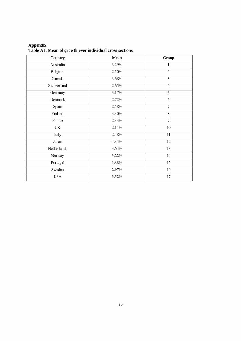
Table 1 reports descriptive statistics for the full sample. The average real economic growth rate recorded

for the 17 OECD countries for the period 1870 to 2013 was 2.95 per cent. Over the sample period, Japan,

Canada and the Netherlands recorded the highest average growth rates of 4.34, 3.68, and 3.64 per cent,

respectively. The average growth rates of Spain, France, Portugal, Switzerland, Italy, UK, Denmark,

Belgium and Spain are all below the sample average growth rate of 2.95 per cent. Netherlands and Italy

recorded the highest growth rate of 70 and 64 per cent, respectively, in 1946, i.e. directly after World War

II. The lowest average growth rate is attributed to Portugal with a rate of only 1.88 per cent.

Table 2 provides the pairwise correlations of the variables in the model. Given the autoregressive nature

of the growth process, the coefficient on gri,t-1 is expected to be positive. According to the Solow growth

model, investment is considered an important driver of economic growth, therefore a positive sign is

expected for liy. Increases in the inflation rate means a rise in the price level, which will lead to a

2 The weblink for the dataset is: http://www.macrohistory.net/data/. 3 http://www.econ.yale.edu/~shiller/data.htm.

12

reduction in consumption and consequently a contraction in output. A negative relationship between

growth and infl is thus expected. The expected sign on government final consumption expenditure

expressed as a share of GDP, lgov, is ambiguous. While a certain level of government expenditure is

necessary to maintain service levels and thus economic growth in a country, excessive government,

especially current spending, will crowd out investment and do little to enhance economic growth of a

country. In the development growth literature, a negative sign is often reported, especially in the case of

developing countries. Government debt to GDP ratio, ldebt, is an indicator of an economy’s health. A

high ratio means an economy is relying on debt to finance its economy and government. Many developed

countries like OECD countries, are characterised by a low debt ratio. This variable is also expected to

have a negative sign indicating the negative impact of high government debt to GDP ratio on productive

capacity.

Table 2: Pairwise correlation

gr l.gr roilunc infl liy lgov ldebt rstockret crisisjst

gr 1 .000

l.gr 0.177** 1.000

roilunc -0.086** -0.006 1.000

infl -0.111** -0.004 -0.025 1.000

liy 0.142** 0.162 -0.127** 0.006 1.000

lgov -0.006 -0.0003 -0.157** 0.228** 0.311** 1.000

ldebt -0.104** -0.123** 0.023 -0.044 -0.210** 0.428** 1.000

rstockret 0.243** 0.055 -0.038 -0.376 -0.002 0.007 0.038 1.000

crisisjst -0.088** -0.011 0.127** -0.012 -0.038 -0.032 0.010 -0.178** 1.000 Notes:*/** denote significance at the 10/5 per cent level

From Table 2, it is evident that l.gr, liy and rstockret are all positively and significantly correlated with

the dependent variable, gr, at the 5 per cent level of significance. A negative and statistically significant

correlation exist between ldebt and gr, crisisjst and gr as well as infl and gr. The correlation between lgov

and gr is close to zero in magnitude and not statistically significant. The fact that we are dealing with a

panel of developed countries here, over a long time span, may explain the marginally positive, although

insignificant relationship. What is of particular interest and importance is the negative correlation of

roilunc with the dependent variable, which is statistically significant at the 5 per cent level. This may be

taken as early evidence in testing the hypothesis that oil price uncertainty may be detrimental to economic

growth for the countries in our sample.

13

5. Empirical Results

In this section we report and compare the results obtained from estimating the specified model in section

3.2 with different panel data techniques. As a baseline model, we estimate the oil price volatility and

economic growth relationship in a one-way fixed effects model specification, see Table 3 column [1].

Based on the Hausman (1978) test for misspecification/endogeneity and three tests for cross-sectional

dependence (Table 4), we proceed to apply dynamic panel estimation techniques to account for

endogeneity originating from correlation between explanatory variables and unobserved country effects,

the Nickell (1981) bias, slope heterogeneity and cross-sectional dependence. Results are presented in

three parts. In the first part, we present the results for the full sample, i.e. 17 OECD countries for the

period 1870 – 2013. This is followed by discussions on the results for the pre-World War II and the post-

World War II subsamples, i.e., for the years 1870 – 1945 and 1946 – 2013, respectively (see Tables 5 to

7).

To determine whether our model is adequately specified or whether endogeneity is present, we use the

Hausman (1978) test. It is expected that the null hypotheses of no misspecification/endogeneity will be

rejected due to the inclusion of the lagged dependant variable in the model. Table 3 below reports the

Hausman test results for the full sample. The Hausman test is rejected at a 1 per cent level of

significance, implying that we reject the null of exogeneity of the independent variables. Even when

omitting the dynamic term from the specification and testing the static model for the presence of

endogeneity, we reject the null of exogeneity. This implies that endogeneity may also originate from

correlation between some of the control variables and unobserved country effects and applying the Bruno

(2005) bias-corrected LSDV estimation technique may potentially still leave the model with a degree of

endogeneity, and thus biased and inconsistent results.

Table 3: Hausman test results

Null Hypothesis Dynamic Model Static Model

H0: E(Xit|uit) = 0 m3(8) = 32.67 m3(7) = 30.94

Decision Reject H0 as p-value <0.0001 Reject H0 as p-value <0.0001 Notes: Rejection of null is an indication of model misspecification/endogeneity.

We also test for the existence of cross-sectional dependence in the panel. The test of Pesaran (2004),

Frees (1995) and Friedman (1937) are reported in Table 4. All three test results are indicative of cross-

sectional dependence.

14

Table 4: Tests for cross-sectional dependence, H0: No cross-sectional dependence

Pesaran (2004) Frees (1995) Friedman (1937)

Z = 26.684 Q = 1.828 χ2=356.554

[0.0000] [0.0000] [0.0000] Note: p-values provided in square brackets

As mentioned earlier, the inclusion of the lagged dependent variable in the model renders fixed effects

more suitable than the random effects estimator, however the fixed effects estimator suffers from the

dynamic panel bias. To control for this, we investigate and experiment with alternative estimators which

are reported in Tables 5 to 7 and discussed below.

Table 5 represents results for the full sample from alternative estimation methods which include the

Bruno (2005) correction for the Nickel (1981) bias, difference GMM with orthogonal deviations

(Arellano and Bover, 1991) which accounts for endogeneity in the model. Table 5 also provides the

estimation output for feasible generalised least squares (FGLS) with cross-section weights and Swamy’s

(1970) random coefficients (RC) regression model, which controls for cross-sectional dependence and

slope heterogeneity.

Column 1 in Table 3 serves as a benchmark to compare with the subsequent alternative estimators

presented in columns 2 to 5. Results across the different estimators are robust, the signs of coefficients

are in line with a priori theoretical expectations and appear overall statistically significant. The negative

impact of real oil price uncertainty on economic growth is significant at the 1 per cent level. It does not

come as a surprise that the estimated parameters for the model using FE, LSDVC and DIF-GMM

estimators are indeed close in magnitude as bias is known to approach zero when T. In this study the

full sample size is 144. According to these estimation results, a 1 unit increase in the realised volatility

measure may detract between 9 and 10 basis points from growth. With an average growth rate of 2.95%

for the countries in the sample over the full sample period, this would imply a reduction in the growth rate

from 2.95% to 2.85% on average. We note however, that the coefficient on real oil price uncertainty is

marginally lower when controlling for slope heterogeneity and cross-sectional dependence, and would

lead to decline in the growth rate of only 5 basis points, that is from 2.95% to 2.9%. Investment and real

stock returns exerts a positive impact on growth, while inflation, debt levels and crisis periods detract

from growth. Government expenditure renders ambiguous results. For the full sample period coefficients

are positive, with the exception Swamy’s RC, and largely insignificant. We know from the empirical

growth literature that the relationship between government expenditure and growth is non-linear, rather

15

than linear, where low levels of government expenditure is necessary for growth, while growing levels of

expenditure may crowd out investment and retract from growth. Note that for the post-World War II

sample, this coefficient turns negative and statistically significant, in line with empirical growth literature.

Table 5: Alternative estimators: FE, LSDV with bias-correction, DIFF-GMM, FGLS, and RC

Full sample, 1870 2013 Dependent variable: gr

[1] FE

LSDV

[2] Bruno’s bias-

corrected LSDV

(LSDVC)

[3] Two-Step DIFF-

GMM with orthogonal deviations

[4] FLGS with

cross-section weights

[5] Swamy’s Random

Coefficients (RC)

l.gr 0.1423*** 0.1508*** 0.2080*** 0.2175*** 0.156***

0.0482 0.0460 0.0605 0.0208 0.0482

roilunc -0.0964*** -0.0962*** -0.0991*** -0.0734*** -0.0517**

0.0184 0.0102 0.0219 0.0122 0.0211

infl -0.2839*** -0.2830*** -0.2474*** -0.1911*** -0.220***

0.0650 0.0187 0.0714 0.0182 0.0629

liy 0.0142*** 0.0142*** 0.0171*** 0.1224*** 0.0257

0.0044 0.0026 0.0047 0.0228 0.0158

lgov 0.0059* 0.0060* 0.0042 0.0005 -0.0044

0.0035 0.0037 0.0037 0.0021 0.0087

ldebt -0.0151*** -0.0149*** -0.0101* -0.0087*** -0.0134*

0.0041 0.0036 0.0054 0.0018 0.0073

rstockret 0.0446*** 0.0445*** 0.0442*** 0.0429*** 0.0502***

0.0079 0.0010 0.0104 0.0051 0.00960

crisisjst -0.0118* -0.0118 -0.0098 -0.0097** -0.0125***

0.0061 0.0130 0.0069 0.0051 0.0214

R2 0.2494 0.2057

F-test F16;1881=2.68 (p=0.0003)

AB(1) Pr > z = 0.003

AB(2) Pr > z = 0.146

Sargan Prob > χ2 = 0.000

Hansen’s J Prob > χ2 = 1.000

Test for parameter constancy

2(112)=426.34 (p=0.0000)

Notes: Standard errors in italics, */**/** denotes significance at the 10/5/1 per cent level; H0 for F-test: H0:1=2=…=N-1=0.

16

We reject the null hypothesis that fixed effects are not significantly different from zero at the 1 per cent

level, with an F-test statistic of 2.68. Furthermore, in the case of the two-step DIF-GMM, the results show

that the null hypothesis for no first-order serial correlation is rejected at the 1 per cent significance level,

however we expected these results as our model is estimated in first differences. We fail to reject the null

hypothesis for second order serial correlation, and we can therefore infer that the error term is free from

first-order serial correlation, thus confirming the consistency of the GMM estimator. The procedure also

reports two diagnostic tests for over-identifying restrictions (i.e. that the moment conditions are correlated

with the disturbance term in the first-differenced equation) namely Hansen’s J test and the Sargan test.

From Hansen’s J test (which is robust to heteroscedasticity and autocorrelation but weakened by many

instruments) we fail to reject the null hypothesis and conclude that the over-identifying restrictions are

valid. The large value p-value of 1.000 is however of concern, which is likely the result of the impact of

the long sample period on the number of instruments used.4 In contrast, from the Sargan test we reject the

null hypothesis of no over-identifying restrictions and infer that the instruments are correlated with the

error term; however, the test is not robust.

In the case of Swamy’s RC model, the test statistic for parameter constancy is strongly rejected,

signifying the need to account for slope heterogeneity in capturing the true result for the panel of

countries. In addition, we are able to conclude which countries in the sample are driving the overall result.

Referring to Table A2 in the Appendix, it is evident that the negative impact of oil price uncertainty is

most notable for oil producing countries, and specifically net oil exporters. The two countries for which

the largest impact is estimated are Norway and Canada, with coefficient values of -0.13 and -0.11

respectively (compared to an overall coefficient for the panel of -0.05).

The overall result is further driven by that of UK and USA, both net importers, but also large-scale oil

producers, with coefficients exceeding the panel average. On the other hand, Japan, France and Sweden

are oil importers, but in fairly large volumes. The coefficients for these countries are also negative,

exceeding the panel average and statistically significant.

The results in Table 6 for the period from 1870 1945 echo those obtained in Table 5; we observe that an

increase in roilunc is both growth deteriorating and highly significant. Based on the magnitude of the

coefficient on roilunc, the impact of uncertainty exerted even a larger negative impact on growth pre-

World War II. According to the estimation results, this means a reduction in the growth rate of between 8

and 12 basis points. This would for example represent a decline from an average of 2.2%, the average

4 Once we analyse the shorter time span of post-World War II period only, the p-value recorded is lower than one, confirming this expectation (see Table 7).

17

growth rate for the pre-World War II period, to between 2.12% and 2.08%. In the case of government

expenditure, once again, although the coefficient of lgov is positive, it is in fact not significantly different

from zero. Thus, there is no evidence that government expenditure stifles economic growth for the pre-

World War II period, as potentially is the case for the post-World War II period. It is significant to note

that one unit decline in realised volatility comparably only detracts between 2.9 and 3 basis points from

the growth rate. With an average growth rate of 3.65% over this period, this would only mean a decline in

the growth rate to 3.62%.

Table 6: Alternative estimators: LSDV with bias-correction, DIFF-GMM and FGLS; pre-World War II, 1870 1945 Dependent variable: gr Variables [1]

FE LSDV

[2] Bruno’s bias-

corrected LSDV (LSDVC)

[3] Two-Step DIFF-GMM

with orthogonal deviations

[4] FLGS with

cross-section weights

l.gr 0.0437 0.0605 0.0650 0.1023***

0.0544 0.0061 0.0602 0.0335

roilunc -0.1264*** -0.1254*** -0.1229*** -0.0811***

0.0343 0.0107 0.0334 0.0219

infl -0.3478*** -0.3460*** -0.3453*** -0.2159***

0.0839 0.0525 0.0799 0.0276

liy 0.0201 0.0202* 0.0148** 0.0939*

0.0089 0.0075 0.0057 0.0563

lgov 0.0104* 0.0106 0.0081 0.0057

0.0049 0.0098 0.0048 0.0045

ldebt -0.0089 -0.0088** -0.0112*** -0.0113**

0.0060 0.0028 0.0038 0.0050

rstockret 0.0615*** 0.0608*** 0.0596** 0.0676***

0.0097 0.0053 0.0259 0.0126

crisisjst -0.0135 -0.0136 -0.0140 -0.0077

0.0256 0.0142 0.0094 0.0076

R2 0.288 0.1644

AB(1) Pr > z = 0.002

AB(2) Pr > z = 0.101

Sargan Prob > χ2 = 0.000

Hansen Prob > χ2 = 1.000

Notes: Standard errors in italics, */**/** denotes significance at the 10/5/1 per cent level.

18

Given the unbalanced nature of the panel and data availability, it is not possible to obtain results for three

countries in the sample using Swamy’s RC model (certain data series for Portugal, Spain and Italy only

starts in the post-World-War II period, and thus results for this estimator are not presented for the

subsample periods.

Table 7: Alternative estimators: LSDV with bias-correction, DIFF-GMM, FGLS, and RC;

post-World War II, 1947 1945 Dependent variable: gr Variables [1]

FE LSDV

[2] Bruno’s

bias-corrected LSDV

(LSDVC)

[3] Two-Step DIFF-

GMM with orthogonal deviations

[4] FLGS with

cross-section weights

l.gr 0.2632*** 0.2763*** 0.3037*** 0.316337***

0.0555 0.0632 0.0458 0.0256

roilunc -0.0285*** -0.0288*** -0.0294*** -0.0317***

0.0092 0.0006 0.0089 0.0124

infl -0.0705 -0.0710*** -0.0766 -0.1261***

0.0607 0.0016 0.0563 0.0226

liy 0.0030 0.0032 0.0018 0.0371

0.0127 0.0156 0.0122 0.0318

lgov -0.0309*** -0.0304*** -0.0289*** -0.0302**

0.0095 0.0045 0.0090 0.0047

ldebt -0.0117*** -0.0115*** -0.0112*** -0.0101***

0.0042 0.0011 0.0040 0.0020

rstockret 0.0485*** 0.0484*** 0.0483*** 0.0415***

0.0106 0.0108 0.0107 0.0043

crisisjst -0.0092 -0.0092*** -0.0091 -0.012**

0.0059 0.0018 0.0058 0.0059

R2 0.2868 0.3583

AB(1) Pr > z = 0.003

AB(2) Pr > z = 0.188

Sargan Prob > χ2 = 0.000

Hansen’s J Prob > χ2 = 0.953

Notes: Standard errors in italics, */**/** denotes significance at the 10/5/1 per cent level.

Note that in all three samples, the coefficient of our variable of interest, roilunc is significant and has the

expected negative sign, meaning real oil price volatility harms economic growth. The control variables

have the expected signs and are all statistically significant except for the government expenditure burden

19

variable, lgov, which is positive and insignificant for the full sample and pre-World War II subsample. As

per Table 7, these results do not hold for the post-World War II subsample for the period between 1946

and 2013; government burden tend to have adverse and significant effects on GDP growth. Overall, while

higher levels of investment are growth enhancing, inflation and government debt tend to have adverse

effects on GDP growth.

6. Conclusion

We investigated the consequences of oil price volatility on real economic growth, measured by growth in

real GDP of 17 main industrialised OECD countries, distinguishing between net oil importing and

exporting countries. Using data from 1870 to 2013, covering two World Wars, oil shocks and periods of

financial crisis, we analyse the relationship by employing a range of panel data estimation techniques

including FE, bias-corrected LSDV, GMM, FGLS and RC. We use the realised volatility in order to

measure the volatility in the world oil price. We divided our sample into two subsamples, namely the pre-

and post-World War II periods. The empirical results from dynamic panel data estimation we obtain are

robust to numerous econometric tests and are broadly consistent with the expectation that the real oil price

volatility is negatively associated with the aggregate economic activity and growth in a panel data

framework.

Moreover, the paper also highlights that the nature and extent of the oil price volatility–economic growth

link varies significantly across the individual countries. It is of interest to note that the country-specific

coefficients for real oil price volatility for the two net oil exporting countries, namely Norway and

Canada, exceeds that of other countries in the sample, indicating an increased sensitivity in economic

performance to adverse developments in terms of uncertainty with respect to oil prices. Oil exporters rely

heavily on their oil revenues which makes them more vulnerable to oil price fluctuation, compared to the

oil importing countries. The estimated sensitivity measure for Norway, is for example almost double that

of the USA, also a large oil producer.

From a policy perspective, oil price volatility clearly impedes economic growth, more so for oil exporters,

and hence policymakers in these economies, and in general, should aim to respond by appropriate design

of expansionary (monetary) policies in the wake of heightened oil market uncertainty. The fact that the

negative influence of oil market volatility on economic activity is weaker in the post-World War II

period, seems to provide some support to the above line of reasoning (Bashar et al., 2013), and also

possibly because oil market uncertainty has declined over time (Baumeister and Peersman, 2013).

20

Appendix Table A1: Mean of growth over individual cross sections

Country Mean Group

Australia 3.29% 1

Belgium 2.50% 2

Canada 3.68% 3

Switzerland 2.65% 4

Germany 3.17% 5

Denmark 2.72% 6

Spain 2.58% 7

Finland 3.30% 8

France 2.33% 9

UK 2.11% 10

Italy 2.48% 11

Japan 4.34% 12

Netherlands 3.64% 13

Norway 3.22% 14

Portugal 1.88% 15

Sweden 2.97% 16

USA 3.32% 17

21

Table A2: Swamy’s (1970) random coefficients results

Country Full sample

1870 2013

post-World War II

1946 2013

roilunc p-value roilunc p-value

Australia -0.0096 0.769 -0.0216 0.174

Belgium -0.0329 0.267 -0.0245 0.117

Canada -0.1072*** 0.000 -0.0405*** 0.010

Switzerland -0.0425 0.137 -0.0336** 0.028

Germany -0.0096 0.735 -0.017 0.275

Denmark -0.0201 0.491 -0.0123 0.420

Spain -0.0352 0.250 -0.0162 0.292

Finland -0.0867*** 0.008 -0.0246* 0.100

France -0.0785** 0.015 -0.0207 0.174

UK -0.0831*** 0.000 -0.0250* 0.080

Italy -0.0348 0.282 0.0030 0.0844

Japan -0.0702** 0.030 -0.0278* 0.062

Netherlands -0.0330 0.249 -0.0023 0.887

Norway -0.1282*** 0.000 -0.0284* 0.072

Portugal 0.0264 0.429 0.0108 0.515

Sweden -0.0655*** 0.008 -0.0330** 0.036

USA -0.0687** 0.030 -0.031* 0.060

Note: */**/*** denote significance at the 10/5/1 per cent level. Due to data availability, these results are not available for all 17 countries in the pre-World War II subsample.

22

References

Akinlo, T. and Apanisile, O.T. (2015). The Impact of Volatility of Oil Price on the Economic Growth in Sub-Saharan Africa. British Journal of Economics, Management & Trade, 5(3): 338-349. Andersen,T., Bollerslev, T. and Meddahi, N. (2003). Analytical evaluation of volatility forecasts. International Economic Review, 45, pp. 1079-1110. Anderson, T.W. and Hsiao, C. (1981). Estimation of Dynamic Models with Error Components. Journal of the American Statistical Association, 76: 598-606. Arellano, M. and Bond, S. (1991). Some Tests of Specification for Panel Data: Monte Carlo Evidence and an Application to Employment Equations. Review of Economic Studies, 58(2): 277-297. Arellano, M. and Bover, O. (1995). Another Look at the Instrumental Variables Estimation of Error-Component Models. Journal of Econometrics, 68: 29-51. Awerbuch , S., and Sauter, R. (2003). Oil price volatility and economic activity: a survey and literature review. IEA Research Paper. Aye. G.C., Dadam, V., Gupta, R. and Mamba, B. (2014). Oil Price uncertainty and manufacturing production. Energy Economics, 43: 41-47. Baltagi, B.H. (2013). Econometric analysis of panel data, 5th ed. John Wiley & Sons Ltd: United Kingdom. Barro, R. (1998). Determinants of economic growth: A cross-country empirical study. Cambridge: The MIT Press. Bashar, O.H.M.N., Mokhtarul Wadud, I.K.M., and Ali Ahmed, H.J. (2013). Oil price uncertainty, monetary policy and the macroeconomy: The Canadian perspective. Economic Modelling, 35, 249–259. Baumeister, C., and Perrsman, G. (2013). The Role of Time-Varying Price Elasticities in Accounting for Volatility Changes in the Crude Oil Market. Journal of Applied Econometrics, 28(7), 1087-1109. Bernanke, B., 1983. Irreversibility, uncertainty, and cyclical investment. Quarterly Journal of Economics, 98, 85–106. Bilgin, M.H., Gozgor, G. and Karabulut, G. (2015). The impact of world energy price volatility on aggregate economic activity in developing Asian economies. Singapore Economic Review, 60(1), 1550009 (20pp). Bjørnland, H.C., Larsen, V.H., and Maih, J. (Forthcoming). Oil and macroeconomic (in)stability. American Economic Journal: Macroeconomics. Blanchard, O.J. and Gali J. (2010). The macroeconomic effects of oil price shocks: Why are the 2000s so different from the 1970s? In International Dimensions of Monetary Policy, J. Gali and M. Gertler (eds.), University of Chicago Press: Chicago: 373–421.

23

Bredin, D., Elder, J., Fountas, S., 2011. Oil volatility and the option value of waiting: an analysis of the G-7. Journal of Futures Markets, 31, 679–702. Bruno, G.F.F. (2005). Approximating the bias of the LSDV estimator for dynamic unbalanced panel data models, Economics Letters, 87: 361-366. Brown, S.P.A. and Yücel, M.C. (2002). Energy Prices and Aggregate Economic Activity: An Interpretative Survey. Quarterly Review of Economics and Finance 42(2): 193–208. Cuñado, J. and Pérez de Gracia, F. (2003). Do oil price shocks matter? Evidence for some European countries, Energy Economics, 25(2): 137-154. De V. Cavalcanti, T.V., Mohaddes, K. and Raissi, M. (2015), Commodity Price Volatility and the Sources of Growth. Journal of Applied Economics, 30: 857-873. El Anshasy, A.A. and Bradley, M.D. (2012). Oil prices and the fiscal policy response in oil exporting countries, Journal of Policy Modeling, 34(5): 605-620. Elder, J., Serletis, A., 2009. Oil price uncertainty in Canada. Energy Economics, 31, 852–856. Elder, J. and Serletis, A (2010). Oil price uncertainty. Journal of Money, Credit and Banking, 42, 1137–1159. Elder, J., Serletis, A., 2011. Volatility in oil prices and manufacturing activity: an investigation of real options. Macroeconomic Dynamics, 15, 379–395. Egwaikhide, F.O. and Omojolaibi, J.A. (2013). A Panel Analysis of Oil Price Dynamics, Fiscal Stance and Macroeconomic Effects: The Case of Some Selected African Countries. Central Bank of Nigeria Economic and Financial Review, 51(1): 61-91. Ferderer, J.P. (1996). Oil price volatility and the macroeconomy. Journal of Macroeconomics, 18(1), 1-26. Frees, E.W. (1995). Assessing cross-sectional correlation in panel data. Journal of Econometrics, 69: 393-414. Friedman, M. (1937). The use of ranks to avoid the assumption of normality implicit in the analysis of variance. Journal of the American Statistical Association, 32: 675-701. Gou, H. and Kliesen, L.K. (2005). Oil Price Volatility and U.S. Macroeconomic Activity. Federal Reserve Bank of St. Port Louis Review. November/December 2005., 87(6): 669-683. Gupta, R., Hollander, H., Wohar, M.E. (forthcoming). The Impact of Oil Shocks in a Small Open Economy New-Keynesian Dynamic Stochastic General Equilibrium Model for South Africa. Emerging Markets Finance and Trade. Hamilton, J. (1983). Oil and the macroeconomy since World War II. Journal of Political Economy, 91: 228-248. Hamilton, J.D. (1985). Historical causes of postwar oil shocks and recessions. The Energy Journal, 1: 97-116.

24

Hamilton, J. (2003). What is an oil shock? Journal of Econometrics, 113(2): 363-398. Hausman, J.A., 1978. Specification Tests in Econometrics. Econometrica, 46(6): 1251-1271. Henry, C., 1974. Investment decisions under uncertainty: the irreversibility effect. American Economic Review, 64, 1006–1012. Hooker, M. (1996). What happened to the oil price macroeconomy relationship? Journal of Monetary Economics, 38: 195-213. Iwayemi, A. and Fowowe, B. (2011). Impact of oil price shocks on selected macroeconomic variables in Nigeria, Energy Policy, 39(2), issue 2: 603-612. Jawad, M., and Khan Niazi, G.S. (2017). Impact of oil price volatility and macroeconomic variables on economic growth in Pakistan. Review of Innovation and Competetiveness, 3(1), 49-74. Jiménez-Rodríguez R. and Sánchez, M., (2005). Oil price shocks and real GDP growth: empirical evidence for some OECD countries. Applied Economics, 37(2): 201-228. Jiménez-Rodríguez R. (2008). The impact of oil price shocks: evidence from the industries of six OECD countries. Energy Economics, 30: 3095-3108. Jordà, Ò., Schularick, M. and Taylor, A.M. (2017). Manufacturing History and the New Business Cycle Facts, in NBER Macroeconomics Annual 2016, 31, edited by M. Eichenbaum and J.A. Parker. Chicago: University of Chicago Press: 213-263. Kiviet, J.F. (1995). On bias, inconsistency and efficiency of various estimators in dynamic panel data models, Journal of Econometrics, 68: 53-78. Lardic, S. and Mignon, V. (2006). The impact of oil prices on GDP in European countries: An empirical investigation based on asymmetric cointegration. Energy Policy, 34(18): 3910-3915. Lardic, S. & Mignon, V. (2008). Oil prices and economic activity: An asymmetric cointegration approach. Energy Economics, 30(3): 847-855. Maghyereh, A.I., Awartani. B., and Sweidan, O.D. (2017). Oil price uncertainty and real output growth: new evidence from selected oil-importing countries in the Middle East. Empirical Economics. https://doi.org/10.1007/s00181-017-1402-7. Mork, K.A. (1989). Oil and Macroeconomy When Prices Go Up and Down: An Extension of Hamilton's Results. Journal of Political Economy, 97(3): 740-744. Mork, K.A., Olsen, O., and Mysen, H.T. (1994). Macroeconomic responses to oil price increases and decreases in seven OECD countries. The Energy Journal, 15(4): 19-36. Mory, J.F. (1993). Oil Prices and Economic Activity: Is the Relationship Symmetric? The Energy Journal, 4:151-162. Nakov, A. and A. Pescatori (2010). Oil and the Great Moderation. Economic Journal 120 (543), 131-156. Nickell, S. (1981). Biases in dynamic models with fixed effects. Econometrica, 49: 1417–1426.

25

Organization of the Petroleum Exporting Countries website. [Online], Available : http://www.opec.org/opec_web/en/about_us/23.htm [Accessed 13 August 2017] Parks, R.W. (1967). Efficient estimation of a system of regression equations when disturbances are both serially and contemporaneously correlated. Journal of the American Statistical Association, 62(318): 500-509. Pesaran, M.H. (2004). General diagnostic tests for cross section dependence in panels. Cambridge Working Papers in Economics No. 0435. University of Cambridge, Faculty of Economics, Pesaran, M.H. and Smith, R.P. (1995). Estimating long-run relationships from dynamic heterogenous panels. Journal of Econometrics, 68(1):79-113. Pesaran, M.H., Shin, Y. and Smith, R.P. (1999). Pooled Mean Group Estimation of Dynamic Heterogeneous Panels, Journal of the American Statistical Association, 94(446): 621-634. Plante, M. and Traum, N. (2012). Time-Varying Oil Price Volatility and Macroeconomic Aggregates. Center for Applied Economics and Policy Research Working Paper No. 2012-002. Center for Applied Economics and Policy Research, Economics Department, Indiana University Bloomington. Plourde, A. and Watkins, G.C. (1998). Crude oil prices between 1985 and 1994: how volatile in relation to other commodities? Resource and Energy Economics, 20(3): 245-262. Rahman, S., Serletis, A., 2010. The asymmetric effects of oil price and monetary policy shocks: a nonlinear VAR approach. Energy Economics, 32, 1460–1466. Rahman, S., Serletis, A., 2011. The asymmetric effects of oil price shocks. Macroeconomic Dynamics, 15, 437–471. Rahman, S., Serletis, A., 2012. Oil price uncertainty and the Canadian economy: evidence from a VARMA, GARCH-in-Mean, asymmetric BEKK model. Energy Economics 34, 603–610. Rentschler, J.E., (2013). Oil price volatility, economic Growth and the hedging role of renewable energy. IMF, Policy Research Working Paper Series No. 6603. Sadorsky, P. (1999). Oil Price Shocks and Stock Market Activity, Energy Economics, 2: 449-469. Swanepoel, J.A. (2006). The impact of external shocks on South African inflation at different price stages, Journal for Studies in Economics and Econometrics, 3(1): 1-22. Swamy, P.A.V.B. (1970). Efficient inference in a random coefficients regression model. Econometrica, 38(2): 311-323. Yoon, K.H., Ratti, R.A., 2011. Energy price uncertainty, energy intensity and firm investment. Energy Economics, 33, 67–78.