Embed Size (px)
Citation preview

Econometrics using STATA
Benjamin MonneryEconomiX, Univ Paris Nanterre
M1 Economie du Droit2017-2018

INTRODUCTION CAUSALITY SOLUTIONS RANDOMIZED EXPERIMENTS
GENERAL INFO
Email : [email protected] : G308A
Schedule : 30 hours• 3-hour whiteboard classes for 7 weeks (G205)• 2-hour computer classes on Stata during 3 weeks (G213B on
13/02 20/02 & 6/03)• one written exam (end of March / early April)
�
class cancelled on January 30
Class in english
Exam in french (or english) on paper
Slides will be available on my webpage
B. Monnery (EconomiX) Econometrics using Stata 2 / 47

INTRODUCTION CAUSALITY SOLUTIONS RANDOMIZED EXPERIMENTS
REFERENCES
> Angrist & Pischke, Mostly Harmless Econometrics, PrincetonUniversity Press
> Cameron & Trivedi, Microeconometrics using Stata, Stata Press
B. Monnery (EconomiX) Econometrics using Stata 3 / 47

INTRODUCTION CAUSALITY SOLUTIONS RANDOMIZED EXPERIMENTS
BONUS READINGS
Bonuses are individual and non-mandatory
This week : chapters 1 & 2 of Mostly Harmless Econometrics“Questions about questions” + “The experimental ideal”
> freely available on my webpage
Goal : make a 1-page critical review of the paper/chapter• brief summary of the paper (topic, method, main points, results)• discuss method, experimental design, interpretations,
conclusions• relate it to the class• criticisms, shortcomings ?
... bonus based on quality/clarity/concision
Send PDF by email before next tuesday (noon)at [email protected]
B. Monnery (EconomiX) Econometrics using Stata 4 / 47
INTRODUCTION CAUSALITY SOLUTIONS RANDOMIZED EXPERIMENTS
CONTENT
Econometrics using STATA
• Use econometric tools to answer policy-relevant questions
... of the cause-and-effect type ( ∂E [y|x ]∂x )
... not predictive modelling (E [y |x ])
• How to answer “theoretically” or intuitivelywhat “model”, what estimator/technique, what design
• How to answer operationally on STATAthe most popular software among (micro)econometricians(others include R, SAS, SPSS...)
B. Monnery (EconomiX) Econometrics using Stata 5 / 47
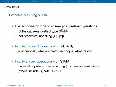
INTRODUCTION CAUSALITY SOLUTIONS RANDOMIZED EXPERIMENTS
B. Monnery (EconomiX) Econometrics using Stata 6 / 47

INTRODUCTION CAUSALITY SOLUTIONS RANDOMIZED EXPERIMENTS
CONTENT
Goal of this course :Learn how to answer empirical questions of the form “what’s theeffect of ... on ... ?” (causal effect identification) using econometrics
• first on paper : illustrated with real-life examples and studies• then on Stata : how to answer by yourself, replicate studies
With a strong emphasis on
• law & economics topics• endogeneity bias or selection• actual practice (how research is done)
... and less so on more theoretical aspects (econometric theory)
Requirement : basics of Econometrics
B. Monnery (EconomiX) Econometrics using Stata 7 / 47

INTRODUCTION CAUSALITY SOLUTIONS RANDOMIZED EXPERIMENTS
Introduction
B. Monnery (EconomiX) Econometrics using Stata 8 / 47
INTRODUCTION CAUSALITY SOLUTIONS RANDOMIZED EXPERIMENTS
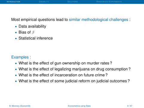
Most empirical questions lead to similar methodological challenges :
• Data availability• Bias of β• Statistical inference
Examples :• What is the effect of gun ownership on murder rates ?• What is the effect of legalizing marijuana on drug consumption ?• What is the effect of incarceration on future crime ?• What is the effect of some judicial reform on judicial outcomes ?
B. Monnery (EconomiX) Econometrics using Stata 9 / 47

INTRODUCTION CAUSALITY SOLUTIONS RANDOMIZED EXPERIMENTS
EVALUATIONS
Public policies employ costly resources to reach social goals
Ex : the CICE tax cut in France�
boost employment, increase competitivity
Ex : cutting class size by two in CP�
improve learning
Types of questions :• Was the policy effective in achieving its goals ?• Did the policy had unintented consequences (positive and
negative) ?• Was the policy cost-effective (Benefit > Cost) ?• Was the policy more efficient than oths (large return per euro B
C ) ?
Answering those questions is called ex-post evaluations�
key parameter is the causal effect of the treatment
B. Monnery (EconomiX) Econometrics using Stata 10 / 47

INTRODUCTION CAUSALITY SOLUTIONS RANDOMIZED EXPERIMENTS
OTHER TYPES OF EVALUATION
Ex-post evaluation can complement -but is not synonym for- othertypes of evaluations :
• Audit : was the policy implemented as planned ?
�
... in terms of target population, take-up, cost, etc.⇒ project management, accounting (not this course)
• Ex-ante evaluation : what effects can we expect if implemented ?
�
more difficult, more uncertain (stronger assumptions)⇒ structural econometrics (not this course)
B. Monnery (EconomiX) Econometrics using Stata 11 / 47
INTRODUCTION CAUSALITY SOLUTIONS RANDOMIZED EXPERIMENTS
STEPS TO ANSWER EMPIRICAL QUESTIONS
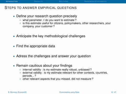
• Define your research question precisely◦ what parameter β do you want to estimate ?◦ is this estimate useful for citizens, policymakers, other researchers, your
company, your customer ?
• Anticipate the key methodological challenges
• Find the appropriate data
• Adress the challenges and answer your question
• Remain cautious about your findings◦ internal validity : is my estimate really robust, unbiased ?◦ external validity : is my estimate relevant for other contexts, countries,
periods... ?◦ other relevant aspects that you missed, did not measure ?
B. Monnery (EconomiX) Econometrics using Stata 12 / 47
INTRODUCTION CAUSALITY SOLUTIONS RANDOMIZED EXPERIMENTS
The Problem(s) With Causality
B. Monnery (EconomiX) Econometrics using Stata 13 / 47
INTRODUCTION CAUSALITY SOLUTIONS RANDOMIZED EXPERIMENTS
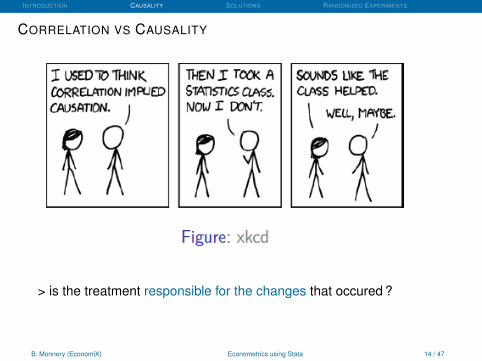
CORRELATION VS CAUSALITY
> is the treatment responsible for the changes that occured ?
B. Monnery (EconomiX) Econometrics using Stata 14 / 47
INTRODUCTION CAUSALITY SOLUTIONS RANDOMIZED EXPERIMENTS
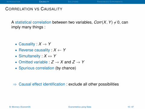
CORRELATION VS CAUSALITY
A statistical correlation between two variables, Corr (X ,Y ) 6= 0, canimply many things :
• Causality : X → Y• Reverse causality : X ← Y• Simultaneity : X ↔ Y• Omitted variable : Z → X and Z → Y• Spurious correlation (by chance)
⇒ Causal effect identification : exclude all other possibilities
B. Monnery (EconomiX) Econometrics using Stata 15 / 47
INTRODUCTION CAUSALITY SOLUTIONS RANDOMIZED EXPERIMENTS
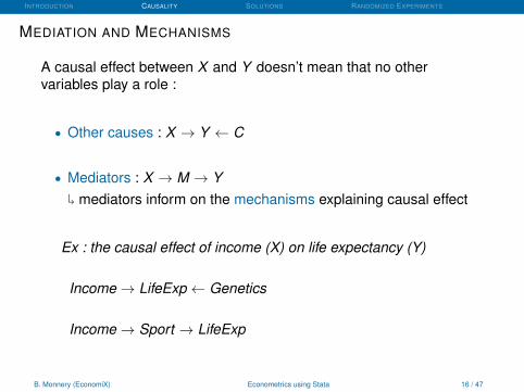
MEDIATION AND MECHANISMS
A causal effect between X and Y doesn’t mean that no othervariables play a role :
• Other causes : X → Y ← C
• Mediators : X → M → Y�
mediators inform on the mechanisms explaining causal effect
Ex : the causal effect of income (X) on life expectancy (Y)
Income→ LifeExp ← Genetics
Income→ Sport → LifeExp
B. Monnery (EconomiX) Econometrics using Stata 16 / 47
INTRODUCTION CAUSALITY SOLUTIONS RANDOMIZED EXPERIMENTS
CAUSALITY AND COUNTERFACTUALS
The quest for causality requires to answer :
What would have happen to Y had the treatment X not occured ?
⇒ refers to some unobservable situation called “counterfactual” (or“potential outcome”)
⇒ Causal effect identification is the art or craft of choosing orconstructing credible counterfactuals (credible estimates of whatwould have happened instead)...
... using experimental or quasi-experimental data
B. Monnery (EconomiX) Econometrics using Stata 17 / 47
INTRODUCTION CAUSALITY SOLUTIONS RANDOMIZED EXPERIMENTS
CAUSALITY AND COUNTERFACTUALS
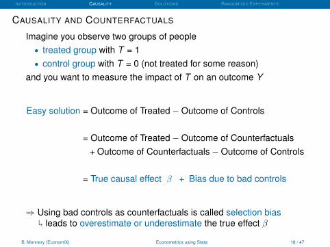
Imagine you observe two groups of people• treated group with T = 1• control group with T = 0 (not treated for some reason)
and you want to measure the impact of T on an outcome Y
Easy solution = Outcome of Treated−Outcome of Controls
= Outcome of Treated−Outcome of Counterfactuals+ Outcome of Counterfactuals−Outcome of Controls
= True causal effect β + Bias due to bad controls
⇒ Using bad controls as counterfactuals is called selection bias�
leads to overestimate or underestimate the true effect β
B. Monnery (EconomiX) Econometrics using Stata 18 / 47
INTRODUCTION CAUSALITY SOLUTIONS RANDOMIZED EXPERIMENTS
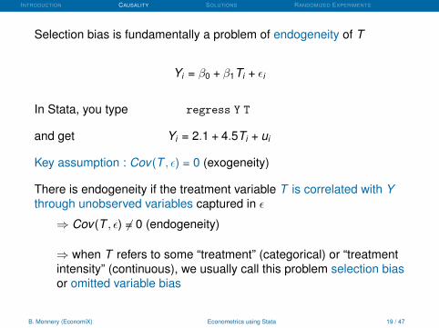
Selection bias is fundamentally a problem of endogeneity of T
Yi = β0 + β1Ti + εi
In Stata, you type regress Y T
and get Yi = 2.1 + 4.5Ti + ui
Key assumption : Cov (T , ε) = 0 (exogeneity)
There is endogeneity if the treatment variable T is correlated with Ythrough unobserved variables captured in ε
⇒ Cov (T , ε) 6= 0 (endogeneity)
⇒ when T refers to some “treatment” (categorical) or “treatmentintensity” (continuous), we usually call this problem selection biasor omitted variable bias
B. Monnery (EconomiX) Econometrics using Stata 19 / 47
INTRODUCTION CAUSALITY SOLUTIONS RANDOMIZED EXPERIMENTS
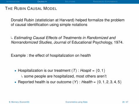
THE RUBIN CAUSAL MODEL
Donald Rubin (statistician at Harvard) helped formalize the problemof causal identification using simple notations
�
Estimating Causal Effects of Treatments in Randomized andNonrandomized Studies, Journal of Educational Psychology, 1974.
Example : the effect of hospitalization on health
• Hospitalization is our treatment (T ) : Hospit = {0,1}
�
some people are hospitalized, most others aren’t• Reported health is our outcome (Y ) : Health = {0,1,2,3,4,5}
B. Monnery (EconomiX) Econometrics using Stata 20 / 47
INTRODUCTION CAUSALITY SOLUTIONS RANDOMIZED EXPERIMENTS
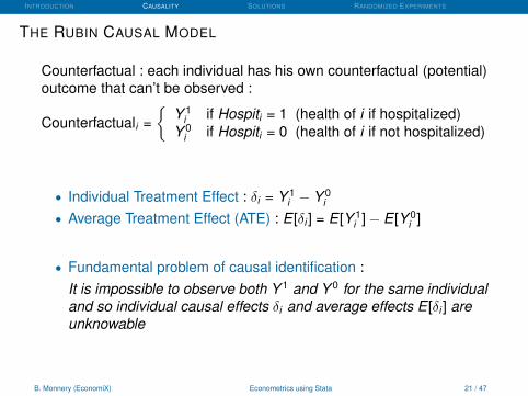
THE RUBIN CAUSAL MODEL
Counterfactual : each individual has his own counterfactual (potential)outcome that can’t be observed :
Counterfactuali ={
Y 1i if Hospiti = 1 (health of i if hospitalized)
Y 0i if Hospiti = 0 (health of i if not hospitalized)
• Individual Treatment Effect : δi = Y 1i − Y 0
i
• Average Treatment Effect (ATE) : E [δi ] = E [Y 1i ]− E [Y 0
i ]
• Fundamental problem of causal identification :It is impossible to observe both Y 1 and Y 0 for the same individualand so individual causal effects δi and average effects E [δi ] areunknowable
B. Monnery (EconomiX) Econometrics using Stata 21 / 47
INTRODUCTION CAUSALITY SOLUTIONS RANDOMIZED EXPERIMENTS
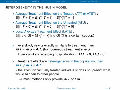
HETEROGENEITY IN THE RUBIN MODEL
• Average Treatment Effect on the Treated (ATT or ATET) :E [δi |T = 1] = E [Y 1
i |T = 1]− E [Y 0i |T = 1]
• Average Treatment Effect on the Unteated (ATU) :E [δi |T = 0] = E [Y 1
i |T = 0]− E [Y 0i |T = 0]
• Local Average Treatment Effect (LATE) :E [δi |i ∈ G] = E [Y 1
i − Y 0i |i ∈ G] (G is a certain subpop)
⇒ If everybody reacts exactly similarly to treatment, thenATT = ATU = ATE (homogeneous treatment effect)
�
very unlikely regarding hospitalization : ATT > 0,ATU = 0
⇒ If treatment effect are heterogeneous in the population, thenATT 6= ATU 6= ATE
�
the effect on “actually treated individuals” does not predict whatwould happen to other people→ most methods only provide ATT or LATE
B. Monnery (EconomiX) Econometrics using Stata 22 / 47
INTRODUCTION CAUSALITY SOLUTIONS RANDOMIZED EXPERIMENTS
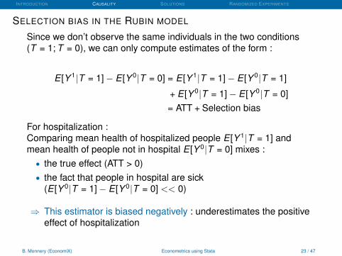
SELECTION BIAS IN THE RUBIN MODEL
Since we don’t observe the same individuals in the two conditions(T = 1; T = 0), we can only compute estimates of the form :
E [Y 1|T = 1]− E [Y 0|T = 0] = E [Y 1|T = 1]− E [Y 0|T = 1]
+ E [Y 0|T = 1]− E [Y 0|T = 0]= ATT + Selection bias
For hospitalization :Comparing mean health of hospitalized people E [Y 1|T = 1] andmean health of people not in hospital E [Y 0|T = 0] mixes :
• the true effect (ATT > 0)• the fact that people in hospital are sick
(E [Y 0|T = 1]− E [Y 0|T = 0] << 0)
⇒ This estimator is biased negatively : underestimates the positiveeffect of hospitalization
B. Monnery (EconomiX) Econometrics using Stata 23 / 47
INTRODUCTION CAUSALITY SOLUTIONS RANDOMIZED EXPERIMENTS
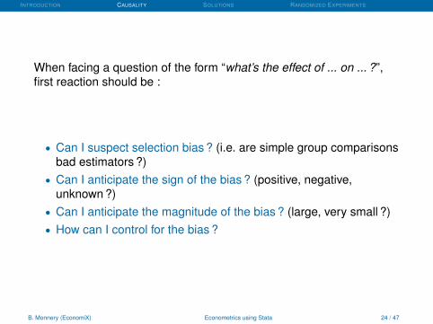
When facing a question of the form “what’s the effect of ... on ... ?”,first reaction should be :
• Can I suspect selection bias ? (i.e. are simple group comparisonsbad estimators ?)
• Can I anticipate the sign of the bias ? (positive, negative,unknown ?)
• Can I anticipate the magnitude of the bias ? (large, very small ?)• How can I control for the bias ?
B. Monnery (EconomiX) Econometrics using Stata 24 / 47

INTRODUCTION CAUSALITY SOLUTIONS RANDOMIZED EXPERIMENTS
AN EXAMPLE WITH PRISONERS AND RECIDIVISM
B. Monnery (EconomiX) Econometrics using Stata 25 / 47

INTRODUCTION CAUSALITY SOLUTIONS RANDOMIZED EXPERIMENTS
Hidden assumption :E [RecidNoPrison|Prison = 1]− E [RecidNoPrison|Prison = 0] = 0
B. Monnery (EconomiX) Econometrics using Stata 26 / 47
INTRODUCTION CAUSALITY SOLUTIONS RANDOMIZED EXPERIMENTS
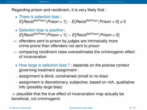
Regarding prison and recidivism, it is very likely that :
• There is selection bias :E [RecidNoPrison|Prison = 1]− E [RecidNoPrison|Prison = 0] 6= 0
• Selection bias is positive :E [RecidNoPrison|Prison = 1] > E [RecidNoPrison|Prison = 0]
⇒ offenders sent to prison by judges are intrinsically morecrime-prone than offenders not sent to prison
⇒ comparing recidivism rates overestimates the criminogenic effectof incarceration
• How large is selection bias ? : depends on the precise contextgoverning treatment assignment :
- assignment is blind, constrained (small to no bias)- assignment is discretionary, subjective, based on rich, qualitative
info (possibly large bias)
⇒ plausible that the true effect of incarceration may actually bebeneficial, not criminogenic
B. Monnery (EconomiX) Econometrics using Stata 27 / 47

INTRODUCTION CAUSALITY SOLUTIONS RANDOMIZED EXPERIMENTS
KEY ASSUMPTION : SUTVASUTVA refers to a key assumption in most evaluations, whatever themethod used
⇒ Stable Unit Treatment-Value Assumption
Incorporates two assumptions :• there is only one treatment : same type, intensity for everybody• assignment of other people to treatment does not affect i ’s
potential outcomesthere is no contagion of treatment effects from treated to
untreated people (no peer effects) orgeneral equilibrum effectsprobably ok for hospitalization (though treatment quality can vary)probably no ok for a large cash transfer program in a village
There are solutions to avoid SUTVA when it doesn’t hold (e.g. look atmore aggregate effects, compare with non-contaminated people...)but we assume SUTVA always holds in this course
B. Monnery (EconomiX) Econometrics using Stata 28 / 47
INTRODUCTION CAUSALITY SOLUTIONS RANDOMIZED EXPERIMENTS
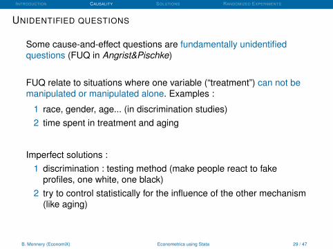
UNIDENTIFIED QUESTIONS
Some cause-and-effect questions are fundamentally unidentifiedquestions (FUQ in Angrist&Pischke)
FUQ relate to situations where one variable (“treatment”) can not bemanipulated or manipulated alone. Examples :
1 race, gender, age... (in discrimination studies)2 time spent in treatment and aging
Imperfect solutions :1 discrimination : testing method (make people react to fake
profiles, one white, one black)2 try to control statistically for the influence of the other mechanism
(like aging)
B. Monnery (EconomiX) Econometrics using Stata 29 / 47

INTRODUCTION CAUSALITY SOLUTIONS RANDOMIZED EXPERIMENTS
Solutions for Identification of Causal Effects
B. Monnery (EconomiX) Econometrics using Stata 30 / 47
INTRODUCTION CAUSALITY SOLUTIONS RANDOMIZED EXPERIMENTS
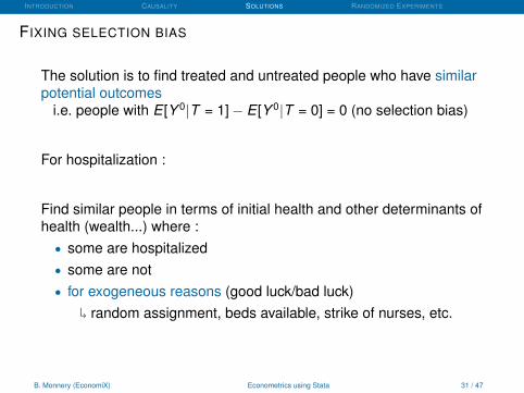
FIXING SELECTION BIAS
The solution is to find treated and untreated people who have similarpotential outcomes
i.e. people with E [Y 0|T = 1]− E [Y 0|T = 0] = 0 (no selection bias)
For hospitalization :
Find similar people in terms of initial health and other determinants ofhealth (wealth...) where :
• some are hospitalized• some are not• for exogeneous reasons (good luck/bad luck)
�
random assignment, beds available, strike of nurses, etc.
B. Monnery (EconomiX) Econometrics using Stata 31 / 47
INTRODUCTION CAUSALITY SOLUTIONS RANDOMIZED EXPERIMENTS
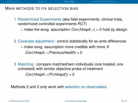
MAIN METHODS TO FIX SELECTION BIAS
1 Randomized Experiments (aka field experiments, clinical trials,randomized controlled experiments RCT)
�
make the exog. assumption Cov (Hospit , ε) = 0 hold by design
2 Covariate-adjustment : control statistically for ex-ante differences
�
make exog. assumption more credible with more XCov (Hospit , ε|PreviousHealth) = 0
3 Matching : compare matched/twin individuals (one treated, oneuntreated) with similar objective proba of treatment
Cov (Hospit , ε|Pr (Hospit)) = 0
Methods 2 and 3 only work with selection on observables
B. Monnery (EconomiX) Econometrics using Stata 32 / 47
INTRODUCTION CAUSALITY SOLUTIONS RANDOMIZED EXPERIMENTS
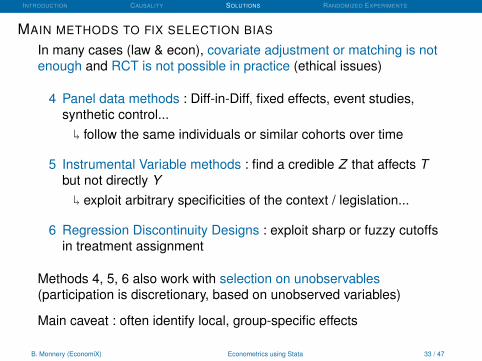
MAIN METHODS TO FIX SELECTION BIAS
In many cases (law & econ), covariate adjustment or matching is notenough and RCT is not possible in practice (ethical issues)
4 Panel data methods : Diff-in-Diff, fixed effects, event studies,synthetic control...
�
follow the same individuals or similar cohorts over time
5 Instrumental Variable methods : find a credible Z that affects Tbut not directly Y
�
exploit arbitrary specificities of the context / legislation...
6 Regression Discontinuity Designs : exploit sharp or fuzzy cutoffsin treatment assignment
Methods 4, 5, 6 also work with selection on unobservables(participation is discretionary, based on unobserved variables)
Main caveat : often identify local, group-specific effects
B. Monnery (EconomiX) Econometrics using Stata 33 / 47

INTRODUCTION CAUSALITY SOLUTIONS RANDOMIZED EXPERIMENTS
Randomized Experiments
B. Monnery (EconomiX) Econometrics using Stata 34 / 47
INTRODUCTION CAUSALITY SOLUTIONS RANDOMIZED EXPERIMENTS
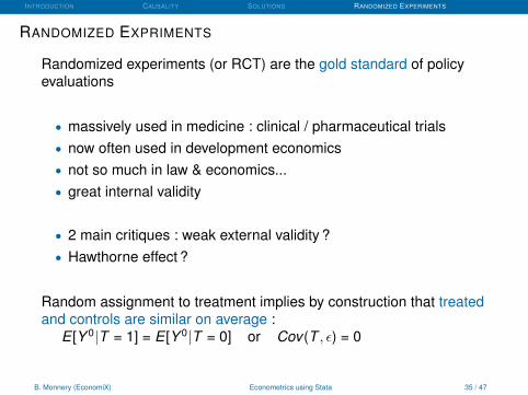
RANDOMIZED EXPRIMENTS
Randomized experiments (or RCT) are the gold standard of policyevaluations
• massively used in medicine : clinical / pharmaceutical trials• now often used in development economics• not so much in law & economics...• great internal validity
• 2 main critiques : weak external validity ?• Hawthorne effect ?
Random assignment to treatment implies by construction that treatedand controls are similar on average :
E [Y 0|T = 1] = E [Y 0|T = 0] or Cov (T , ε) = 0
B. Monnery (EconomiX) Econometrics using Stata 35 / 47
INTRODUCTION CAUSALITY SOLUTIONS RANDOMIZED EXPERIMENTS
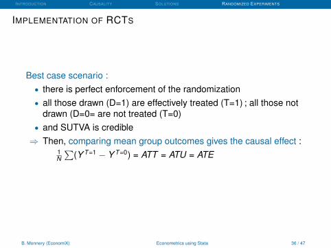
IMPLEMENTATION OF RCTS
Best case scenario :• there is perfect enforcement of the randomization• all those drawn (D=1) are effectively treated (T=1) ; all those not
drawn (D=0= are not treated (T=0)• and SUTVA is credible⇒ Then, comparing mean group outcomes gives the causal effect :
1N
∑(Y T=1 − Y T=0) = ATT = ATU = ATE
B. Monnery (EconomiX) Econometrics using Stata 36 / 47
INTRODUCTION CAUSALITY SOLUTIONS RANDOMIZED EXPERIMENTS
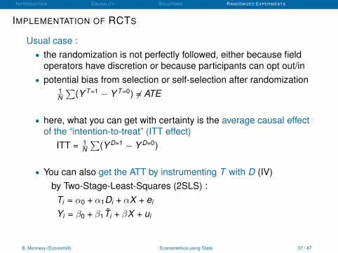
IMPLEMENTATION OF RCTS
Usual case :• the randomization is not perfectly followed, either because field
operators have discretion or because participants can opt out/in• potential bias from selection or self-selection after randomization
1N
∑(Y T=1 − Y T=0) 6= ATE
• here, what you can get with certainty is the average causal effectof the “intention-to-treat” (ITT effect)
ITT = 1N
∑(Y D=1 − Y D=0)
• You can also get the ATT by instrumenting T with D (IV)by Two-Stage-Least-Squares (2SLS) :
Ti = α0 + α1Di + αX + ei
Yi = β0 + β1T̂i + βX + ui
B. Monnery (EconomiX) Econometrics using Stata 37 / 47
INTRODUCTION CAUSALITY SOLUTIONS RANDOMIZED EXPERIMENTS
IMPLEMENTATION OF RCTS
Imbens (2009) : ... in a situation where one has control over theassignment mechanism, there is little to gain, and much to lose, bygiving that up through allowing individuals to choose their owntreatment regime. Randomization ensures exogeneity of keyvariables, where in a corresponding observational study one wouldhave to worry about their endogeneity.
When individuals can self-select (or be selected) after randomization,the RCT is still very useful but data analysis requires precaution andregression techniques (no simple mean comparisons)
In any case, need to check balancing of key variables across the twogroups : in expectations, treated and controls should be similar oneach observed variable
B. Monnery (EconomiX) Econometrics using Stata 38 / 47

INTRODUCTION CAUSALITY SOLUTIONS RANDOMIZED EXPERIMENTS
BONUS 2Bonuses are individual and non-mandatory
This week : Killias et al. (2010) How damaging is imprisonment in thelong-term ? A controlled experiment comparing long-term effects ofcommunity service and short custodial sentences on re-offending andsocial integration
> available on my webpage
Goal : make a 1-page critical review of the paper/chapter• brief summary of the paper (topic, method, main points, results)• discuss method, experimental design, interpretations,
conclusions• relate it to the class• criticisms, shortcomings ?
... bonus based on quality/clarity/concision
Send PDF by email before next monday (noon)at [email protected]
B. Monnery (EconomiX) Econometrics using Stata 39 / 47
INTRODUCTION CAUSALITY SOLUTIONS RANDOMIZED EXPERIMENTS
FROM EXPERIMENTS TO REGRESSIONS
Even perfectly enforced RCTs can / should be analysed usingeconometrics. Why ?
1. natural link between “potential outcomes” and regressions2. regressions can easily include covariates- to account for the design of the experiment (stratification)- to make sub-group analysis, interaction effects- to increase precision of the causal estimate
3. regressions can deal with inference issues- heteroscedasticity, autocorrelation of errors...
B. Monnery (EconomiX) Econometrics using Stata 40 / 47
INTRODUCTION CAUSALITY SOLUTIONS RANDOMIZED EXPERIMENTS
FROM EXPERIMENTS TO REGRESSIONS
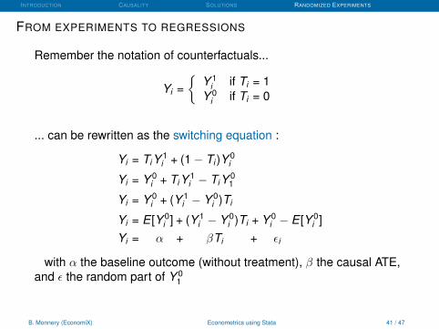
Remember the notation of counterfactuals...
Yi ={
Y 1i if Ti = 1
Y 0i if Ti = 0
... can be rewritten as the switching equation :
Yi = TiY 1i + (1− Ti )Y 0
i
Yi = Y 0i + TiY 1
i − TiY 01
Yi = Y 0i + (Y 1
i − Y 0i )Ti
Yi = E [Y 0i ] + (Y 1
i − Y 0i )Ti + Y 0
i − E [Y 0i ]
Yi = α + βTi + εi
with α the baseline outcome (without treatment), β the causal ATE,and ε the random part of Y 0
1
B. Monnery (EconomiX) Econometrics using Stata 41 / 47
INTRODUCTION CAUSALITY SOLUTIONS RANDOMIZED EXPERIMENTS
FROM EXPERIMENTS TO REGRESSIONS
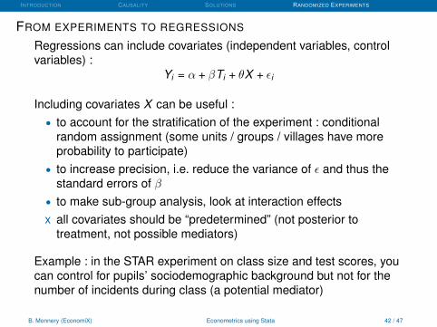
Regressions can include covariates (independent variables, controlvariables) :
Yi = α + βTi + θX + εi
Including covariates X can be useful :• to account for the stratification of the experiment : conditional
random assignment (some units / groups / villages have moreprobability to participate)
• to increase precision, i.e. reduce the variance of ε and thus thestandard errors of β
• to make sub-group analysis, look at interaction effectsx all covariates should be “predetermined” (not posterior to
treatment, not possible mediators)
Example : in the STAR experiment on class size and test scores, youcan control for pupils’ sociodemographic background but not for thenumber of incidents during class (a potential mediator)
B. Monnery (EconomiX) Econometrics using Stata 42 / 47
INTRODUCTION CAUSALITY SOLUTIONS RANDOMIZED EXPERIMENTS
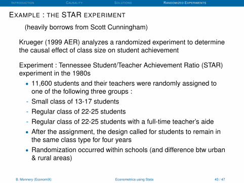
EXAMPLE : THE STAR EXPERIMENT
(heavily borrows from Scott Cunningham)
Krueger (1999 AER) analyzes a randomized experiment to determinethe causal effect of class size on student achievement
Experiment : Tennessee Student/Teacher Achievement Ratio (STAR)experiment in the 1980s
• 11,600 students and their teachers were randomly assigned toone of the following three groups :
- Small class of 13-17 students- Regular class of 22-25 students- Regular class of 22-25 students with a full-time teacher’s aide• After the assignment, the design called for students to remain in
the same class type for four years• Randomization occurred within schools (and difference btw urban
& rural areas)
B. Monnery (EconomiX) Econometrics using Stata 43 / 47
INTRODUCTION CAUSALITY SOLUTIONS RANDOMIZED EXPERIMENTS
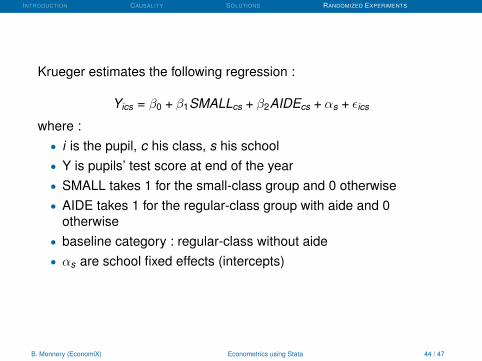
Krueger estimates the following regression :
Yics = β0 + β1SMALLcs + β2AIDEcs + αs + εics
where :• i is the pupil, c his class, s his school• Y is pupils’ test score at end of the year• SMALL takes 1 for the small-class group and 0 otherwise• AIDE takes 1 for the regular-class group with aide and 0
otherwise• baseline category : regular-class without aide• αs are school fixed effects (intercepts)
B. Monnery (EconomiX) Econometrics using Stata 44 / 47

INTRODUCTION CAUSALITY SOLUTIONS RANDOMIZED EXPERIMENTS
Regression results from OLS on kindergarden test scores(percentiles) :
B. Monnery (EconomiX) Econometrics using Stata 45 / 47

INTRODUCTION CAUSALITY SOLUTIONS RANDOMIZED EXPERIMENTS
Replication on Stata...
B. Monnery (EconomiX) Econometrics using Stata 46 / 47
Econometrics using STATA
Benjamin MonneryEconomiX, Univ Paris Nanterre
M1 Economie du Droit2017-2018