Embed Size (px)
Citation preview
ECONOMETRICS
Bruce E. Hansen
c°2000, 2001, 2002, 2003, 2004, 20051
University of Wisconsin
www.ssc.wisc.edu/~bhansen
Revised: January 2005
Comments Welcome
1This manuscript may be printed and reproduced for individual or instructional use, but may not be
printed for commercial purposes.
Contents
1 Regression and Projection 2
1.1 Random Sample . . . . . . . . . . . . . . . . . . . . . . . . . . . . . . . . . . . . . 2
1.2 Observational Data . . . . . . . . . . . . . . . . . . . . . . . . . . . . . . . . . . . . 2
1.3 Conditional Mean . . . . . . . . . . . . . . . . . . . . . . . . . . . . . . . . . . . . . 3
1.4 Regression Equation . . . . . . . . . . . . . . . . . . . . . . . . . . . . . . . . . . . 4
1.5 Conditional Variance . . . . . . . . . . . . . . . . . . . . . . . . . . . . . . . . . . . 6
1.6 Best Linear Predictor . . . . . . . . . . . . . . . . . . . . . . . . . . . . . . . . . . 7
2 Least Squares Estimation 11
2.1 Estimation . . . . . . . . . . . . . . . . . . . . . . . . . . . . . . . . . . . . . . . . 11
2.2 Least Squares . . . . . . . . . . . . . . . . . . . . . . . . . . . . . . . . . . . . . . . 12
2.3 Model in Matrix Notation . . . . . . . . . . . . . . . . . . . . . . . . . . . . . . . . 13
2.4 Residual Regression . . . . . . . . . . . . . . . . . . . . . . . . . . . . . . . . . . . 15
2.5 Efficiency . . . . . . . . . . . . . . . . . . . . . . . . . . . . . . . . . . . . . . . . . 17
2.6 Consistency . . . . . . . . . . . . . . . . . . . . . . . . . . . . . . . . . . . . . . . . 18
2.7 Asymptotic Normality . . . . . . . . . . . . . . . . . . . . . . . . . . . . . . . . . . 19
2.8 Covariance Matrix Estimation . . . . . . . . . . . . . . . . . . . . . . . . . . . . . . 20
2.9 Multicollinearity . . . . . . . . . . . . . . . . . . . . . . . . . . . . . . . . . . . . . 22
2.10 Omitted Variables . . . . . . . . . . . . . . . . . . . . . . . . . . . . . . . . . . . . 23
2.11 Irrelevant Variables . . . . . . . . . . . . . . . . . . . . . . . . . . . . . . . . . . . . 24
2.12 Functions of Parameters . . . . . . . . . . . . . . . . . . . . . . . . . . . . . . . . . 25
2.13 t tests . . . . . . . . . . . . . . . . . . . . . . . . . . . . . . . . . . . . . . . . . . . 26
2.14 Confidence Intervals . . . . . . . . . . . . . . . . . . . . . . . . . . . . . . . . . . . 27
2.15 Wald Tests . . . . . . . . . . . . . . . . . . . . . . . . . . . . . . . . . . . . . . . . 28
2.16 F Tests . . . . . . . . . . . . . . . . . . . . . . . . . . . . . . . . . . . . . . . . . . 29
2.17 Problems with Tests of NonLinear Hypotheses . . . . . . . . . . . . . . . . . . . . 31
2.18 Monte Carlo Simulation . . . . . . . . . . . . . . . . . . . . . . . . . . . . . . . . . 34
2.19 Estimating a Wage Equation . . . . . . . . . . . . . . . . . . . . . . . . . . . . . . 36
3 Regression Estimation 39
3.1 Linear Regression . . . . . . . . . . . . . . . . . . . . . . . . . . . . . . . . . . . . . 39
3.2 Bias and Variance of OLS estimator . . . . . . . . . . . . . . . . . . . . . . . . . . 39
3.3 Forecast Intervals . . . . . . . . . . . . . . . . . . . . . . . . . . . . . . . . . . . . . 41
3.4 Normal Regression Model . . . . . . . . . . . . . . . . . . . . . . . . . . . . . . . . 42
3.5 GLS and the Gauss-Markov Theorem . . . . . . . . . . . . . . . . . . . . . . . . . 44
3.6 Least Absolute Deviations . . . . . . . . . . . . . . . . . . . . . . . . . . . . . . . . 46
3.7 NonLinear Least Squares . . . . . . . . . . . . . . . . . . . . . . . . . . . . . . . . 48
i
3.8 Testing for Omitted NonLinearity . . . . . . . . . . . . . . . . . . . . . . . . . . . . 50
3.9 Model Selection . . . . . . . . . . . . . . . . . . . . . . . . . . . . . . . . . . . . . . 51
4 The Bootstrap 55
4.1 Definition of the Bootstrap . . . . . . . . . . . . . . . . . . . . . . . . . . . . . . . 55
4.2 The Empirical Distribution Function . . . . . . . . . . . . . . . . . . . . . . . . . . 56
4.3 Nonparametric Bootstrap . . . . . . . . . . . . . . . . . . . . . . . . . . . . . . . . 57
4.4 Bootstrap Estimation of Bias and Variance . . . . . . . . . . . . . . . . . . . . . . 57
4.5 Percentile Intervals . . . . . . . . . . . . . . . . . . . . . . . . . . . . . . . . . . . . 59
4.6 Percentile-t Equal-Tailed Interval . . . . . . . . . . . . . . . . . . . . . . . . . . . . 60
4.7 Symmetric Percentile-t Intervals . . . . . . . . . . . . . . . . . . . . . . . . . . . . 61
4.8 Asymptotic Expansions . . . . . . . . . . . . . . . . . . . . . . . . . . . . . . . . . 62
4.9 One-Sided Tests . . . . . . . . . . . . . . . . . . . . . . . . . . . . . . . . . . . . . 63
4.10 Symmetric Two-Sided Tests . . . . . . . . . . . . . . . . . . . . . . . . . . . . . . . 64
4.11 Percentile Confidence Intervals . . . . . . . . . . . . . . . . . . . . . . . . . . . . . 65
4.12 Bootstrap Methods for Regression Models . . . . . . . . . . . . . . . . . . . . . . . 66
5 Generalized Method of Moments 68
5.1 Overidentified Linear Model . . . . . . . . . . . . . . . . . . . . . . . . . . . . . . . 68
5.2 GMM Estimator . . . . . . . . . . . . . . . . . . . . . . . . . . . . . . . . . . . . . 69
5.3 Distribution of GMM Estimator . . . . . . . . . . . . . . . . . . . . . . . . . . . . 69
5.4 Estimation of the Efficient Weight Matrix . . . . . . . . . . . . . . . . . . . . . . . 70
5.5 GMM: The General Case . . . . . . . . . . . . . . . . . . . . . . . . . . . . . . . . 71
5.6 Over-Identification Test . . . . . . . . . . . . . . . . . . . . . . . . . . . . . . . . . 72
5.7 Hypothesis Testing: The Distance Statistic . . . . . . . . . . . . . . . . . . . . . . 73
5.8 Conditional Moment Restrictions . . . . . . . . . . . . . . . . . . . . . . . . . . . . 74
5.9 Bootstrap GMM Inference . . . . . . . . . . . . . . . . . . . . . . . . . . . . . . . . 75
5.10 Generalized Least Squares . . . . . . . . . . . . . . . . . . . . . . . . . . . . . . . . 76
5.10.1 Skedastic Regression . . . . . . . . . . . . . . . . . . . . . . . . . . . . . . . 76
5.10.2 Estimation of Skedastic Regression . . . . . . . . . . . . . . . . . . . . . . . 76
5.10.3 Testing for Heteroskedasticity . . . . . . . . . . . . . . . . . . . . . . . . . . 77
5.10.4 Feasible GLS Estimation . . . . . . . . . . . . . . . . . . . . . . . . . . . . 78
6 Empirical Likelihood 80
6.1 Non-Parametric Likelihood . . . . . . . . . . . . . . . . . . . . . . . . . . . . . . . 80
6.2 Asymptotic Distribution of EL Estimator . . . . . . . . . . . . . . . . . . . . . . . 82
6.3 Overidentifying Restrictions . . . . . . . . . . . . . . . . . . . . . . . . . . . . . . . 83
6.4 Testing . . . . . . . . . . . . . . . . . . . . . . . . . . . . . . . . . . . . . . . . . . . 84
6.5 Numerical Computation . . . . . . . . . . . . . . . . . . . . . . . . . . . . . . . . . 84
6.5.1 Derivatives . . . . . . . . . . . . . . . . . . . . . . . . . . . . . . . . . . . . 85
6.5.2 Inner Loop . . . . . . . . . . . . . . . . . . . . . . . . . . . . . . . . . . . . 85
6.5.3 Outer Loop . . . . . . . . . . . . . . . . . . . . . . . . . . . . . . . . . . . . 86
7 Endogeneity 87
7.1 Instrumental Variables . . . . . . . . . . . . . . . . . . . . . . . . . . . . . . . . . . 88
7.2 Reduced Form . . . . . . . . . . . . . . . . . . . . . . . . . . . . . . . . . . . . . . 89
7.3 Identification . . . . . . . . . . . . . . . . . . . . . . . . . . . . . . . . . . . . . . . 90
7.4 Estimation . . . . . . . . . . . . . . . . . . . . . . . . . . . . . . . . . . . . . . . . 90
ii
7.5 Special Cases: IV and 2SLS . . . . . . . . . . . . . . . . . . . . . . . . . . . . . . . 91
7.6 Bekker Asymptotics . . . . . . . . . . . . . . . . . . . . . . . . . . . . . . . . . . . 92
7.7 Identification Failure . . . . . . . . . . . . . . . . . . . . . . . . . . . . . . . . . . . 93
8 Univariate Time Series 96
8.1 Stationarity and Ergodicity . . . . . . . . . . . . . . . . . . . . . . . . . . . . . . . 96
8.2 Autoregressions . . . . . . . . . . . . . . . . . . . . . . . . . . . . . . . . . . . . . . 98
8.3 Stationarity of AR(1) Process . . . . . . . . . . . . . . . . . . . . . . . . . . . . . . 98
8.4 Lag Operator . . . . . . . . . . . . . . . . . . . . . . . . . . . . . . . . . . . . . . . 99
8.5 Stationarity of AR(k) . . . . . . . . . . . . . . . . . . . . . . . . . . . . . . . . . . 99
8.6 Estimation . . . . . . . . . . . . . . . . . . . . . . . . . . . . . . . . . . . . . . . . 100
8.7 Asymptotic Distribution . . . . . . . . . . . . . . . . . . . . . . . . . . . . . . . . . 101
8.8 Bootstrap for Autoregressions . . . . . . . . . . . . . . . . . . . . . . . . . . . . . . 101
8.9 Trend Stationarity . . . . . . . . . . . . . . . . . . . . . . . . . . . . . . . . . . . . 102
8.10 Testing for Omitted Serial Correlation . . . . . . . . . . . . . . . . . . . . . . . . . 103
8.11 Model Selection . . . . . . . . . . . . . . . . . . . . . . . . . . . . . . . . . . . . . . 103
8.12 Autoregressive Unit Roots . . . . . . . . . . . . . . . . . . . . . . . . . . . . . . . . 104
9 Multivariate Time Series 106
9.1 Vector Autoregressions (VARs) . . . . . . . . . . . . . . . . . . . . . . . . . . . . . 106
9.2 Estimation . . . . . . . . . . . . . . . . . . . . . . . . . . . . . . . . . . . . . . . . 107
9.3 Restricted VARs . . . . . . . . . . . . . . . . . . . . . . . . . . . . . . . . . . . . . 107
9.4 Single Equation from a VAR . . . . . . . . . . . . . . . . . . . . . . . . . . . . . . 108
9.5 Testing for Omitted Serial Correlation . . . . . . . . . . . . . . . . . . . . . . . . . 108
9.6 Selection of Lag Length in an VAR . . . . . . . . . . . . . . . . . . . . . . . . . . . 109
9.7 Granger Causality . . . . . . . . . . . . . . . . . . . . . . . . . . . . . . . . . . . . 109
9.8 Cointegration . . . . . . . . . . . . . . . . . . . . . . . . . . . . . . . . . . . . . . . 110
9.9 Cointegrated VARs . . . . . . . . . . . . . . . . . . . . . . . . . . . . . . . . . . . . 110
10 Limited Dependent Variables 112
10.1 Binary Choice . . . . . . . . . . . . . . . . . . . . . . . . . . . . . . . . . . . . . . . 112
10.2 Count Data . . . . . . . . . . . . . . . . . . . . . . . . . . . . . . . . . . . . . . . . 114
10.3 Censored Data . . . . . . . . . . . . . . . . . . . . . . . . . . . . . . . . . . . . . . 114
10.4 Sample Selection . . . . . . . . . . . . . . . . . . . . . . . . . . . . . . . . . . . . . 115
11 Panel Data 118
11.1 Individual-Effects Model . . . . . . . . . . . . . . . . . . . . . . . . . . . . . . . . . 118
11.2 Fixed Effects . . . . . . . . . . . . . . . . . . . . . . . . . . . . . . . . . . . . . . . 118
11.3 Dynamic Panel Regression . . . . . . . . . . . . . . . . . . . . . . . . . . . . . . . . 120
12 Nonparametrics 121
12.1 Kernel Density Estimation . . . . . . . . . . . . . . . . . . . . . . . . . . . . . . . . 121
12.2 Asymptotic MSE for Kernel Estimates . . . . . . . . . . . . . . . . . . . . . . . . . 123
A Mathematical Formula 126
iii
B Matrix Algebra 128
B.1 Terminology . . . . . . . . . . . . . . . . . . . . . . . . . . . . . . . . . . . . . . . . 128
B.2 Matrix Multiplication . . . . . . . . . . . . . . . . . . . . . . . . . . . . . . . . . . 129
B.3 Trace, Inverse, Determinant . . . . . . . . . . . . . . . . . . . . . . . . . . . . . . . 130
B.4 Eigenvalues . . . . . . . . . . . . . . . . . . . . . . . . . . . . . . . . . . . . . . . . 132
B.5 Idempotent and Projection Matrices . . . . . . . . . . . . . . . . . . . . . . . . . . 133
B.6 Kronecker Products and the Vec Operator . . . . . . . . . . . . . . . . . . . . . . . 135
B.7 Matrix Calculus . . . . . . . . . . . . . . . . . . . . . . . . . . . . . . . . . . . . . . 136
C Probability 137
C.1 Foundations . . . . . . . . . . . . . . . . . . . . . . . . . . . . . . . . . . . . . . . . 137
C.2 Random Variables . . . . . . . . . . . . . . . . . . . . . . . . . . . . . . . . . . . . 139
C.3 Expectation . . . . . . . . . . . . . . . . . . . . . . . . . . . . . . . . . . . . . . . . 139
C.4 Common Distributions . . . . . . . . . . . . . . . . . . . . . . . . . . . . . . . . . . 140
C.5 Multivariate Random Variables . . . . . . . . . . . . . . . . . . . . . . . . . . . . . 143
C.6 Conditional Distributions and Expectation . . . . . . . . . . . . . . . . . . . . . . . 145
C.7 Transformations . . . . . . . . . . . . . . . . . . . . . . . . . . . . . . . . . . . . . 146
C.8 Normal and Related Distributions . . . . . . . . . . . . . . . . . . . . . . . . . . . 147
C.9 Maximum Likelihood . . . . . . . . . . . . . . . . . . . . . . . . . . . . . . . . . . . 150
D Asymptotic Theory 154
D.1 Inequalities . . . . . . . . . . . . . . . . . . . . . . . . . . . . . . . . . . . . . . . . 154
D.2 Convergence in Probability . . . . . . . . . . . . . . . . . . . . . . . . . . . . . . . 156
D.3 Almost Sure Convergence . . . . . . . . . . . . . . . . . . . . . . . . . . . . . . . . 157
D.4 Convergence in Distribution . . . . . . . . . . . . . . . . . . . . . . . . . . . . . . . 159
D.5 Asymptotic Transformations . . . . . . . . . . . . . . . . . . . . . . . . . . . . . . . 161
E Numerical Optimization 162
E.1 Grid Search . . . . . . . . . . . . . . . . . . . . . . . . . . . . . . . . . . . . . . . . 162
E.2 Gradient Methods . . . . . . . . . . . . . . . . . . . . . . . . . . . . . . . . . . . . 163
E.3 Derivative-Free Methods . . . . . . . . . . . . . . . . . . . . . . . . . . . . . . . . . 164
1
Chapter 1
Regression and Projection
1.1 Random Sample
An econometrician has observational data
(y1, x1) , (y2, x2) , ..., (yi, xi) , ..., (yn, xn) = (yi, xi) : i = 1, ..., nwhere each pair yi, xi ∈ R × Rk is an observation on an individual (e.g., household or firm).
We call these observations the sample.
If the data is cross-sectional (each observation is a different individual) it is often reasonable
to assume they are mutually independent. If the data is randomly gathered, it is reasonable to
model each observation as a random draw from the same probability distribution. In this case the
data are independent and identically distributed, or iid. We call this a random sample.
Sometimes the independent part of the label iid is misconstrued. It is not a statement about the
relationship between yi and xi. Rather it means that the pair (yi, xi) is independent of the pair(yj , xj) for i 6= j.
The random variables (yi, xi) have a distribution F which we call the population. This
“population” is infinitely large. This abstraction can a source of confusion as it does not correspond
to a physical population in the real real. The distribution F is unknown, and the goal of statistical
inference is to learn about features of F from the sample.
Notice that the observations are paired (yi, xi). We call yi the dependent variable. We callxi alternatively the regressor, the conditioning variable, or the covariates. We can list the
elements of xi in the vector
xi =
⎛⎜⎜⎜⎝x1ix2i...
xki
⎞⎟⎟⎟⎠ .
At this point in our analysis it is unimportant whether the observations yi and xi may come
from continuous or discrete distributions. For example, many regressors in econometric practice
are binary, taking on only the values 0 and 1, and are typically called dummy variables.
1.2 Observational Data
A common econometric question is to quantify the impact of xi on yi. For example, a concern
in labor economics is the returns to schooling — the change in earnings induced by increasing a
2
worker’s education, holding other variables constant. Another issue of interest is the earnings gap
between men and women. In these examples, yi might be wages and xi could include gender, race,
education, and experience.
Ideally, we would use experimental data to answer these questions. To measure the returns
to schooling, an experiment might randomly divide children into groups, mandate different levels
of education to the different groups, and then follow the children’s wage path as they mature and
enter the labor force. The differences between the groups could be attributed to the different levels
of education. However, experiments such as this are infeasible, even immoral!
Instead, most economic data is observational. To continue the above example, what we
observe (through data collection) is the level of a person’s education and their wage. We can
thus measure the joint distribution of these variables, and assess the joint dependence. But we
cannot infer causality, as we are not able to manipulate one variable to see the direct effect on the
other. For example, a person’s level of education is (at least partially) determined by that person’s
choices and their personal achievement in education. These factors are likely to be affected by their
personal abilities and attitudes towards work. The fact that a person is highly education suggest
a high level of ability. This is an alternative explanation for the positive correlation between
educational levels and wages. High ability individuals do better in school, and therefore choose to
attain higher levels of education, and their high ability is the fundamental reason for their high
wages. The point is that multiple explanations are consistent with a positive correlation between
schooling levels and education. Knowledge of the joint distibution cannot distinguish between
these explanations.
This discussion means that causality cannot be infered from observational data alone. Causal
inference requires identification, and this is based on strong assumptions. We will return to a
discussion of some of these issues in Chapter 7.
1.3 Conditional Mean
To study how the distribution of yi varies with the variables xi in the population, we can focus on
f (y | x) , the conditional density of yi given xi. This is well defined whether or not the effect of xion yi is causal or observational.
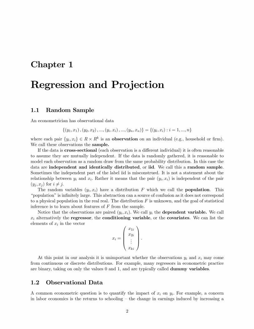
To illustrate, Figure 1.1 displays the density1 of hourly wages for men and women. The
population is Caucasian non-military wage earners with a college degree and 10-15 years of potential
work experience. These are conditional density functions — the density of hourly wages conditional
on race, gender, education and experience. The two density curves show the effect of gender on
the distribution of wages, holding the other variables constant.
While it is easy to observe that the two densities are unequal, it is useful to have numerical
measures of the difference. An important summary measure is the conditional mean
m(x) = E (yi | xi = x) =
Z ∞
−∞yf (y | x)dy. (1.1)
In general, m(x) can take any form, and exists so long as E |yi| <∞. In the example presented in
Figure 1.1, the mean wage for men is $26.81, and that for women is $20.33. These are indicated
in Figure 1.1 by the arrows drawn to the x-axis.
The comparison in Figure 1.1 is facilitated by the fact that the control variable (gender) is
discrete. When the distribution of the control variable is continuous, then comparisons become
1These are nonparametric density estimates using a Gaussian kernel with the bandwidth selected by cross-
validation. See Chapter 12. The data are from the 2004 Current Population Survey
3
Figure 1.1: Wage Distribution for Caucasian College Grads with 10-15 Years Work Experience
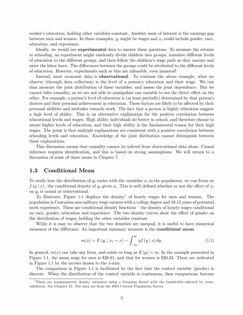
more complicated. To illustrate, Figure 1.2 displays a scatter plot2 of wages against education
levels. Assuming for simplicity that this is the true joint distribution, the solid line displays the
conditional expectation of wages varying with education. The conditional expectation function is
close to linear; the dashed line is a linear projection approximation which will be discussed in the
next section. The main point to be learned from Figure 1.2 is how the conditional expectation
describes an important feature of the conditional distribution. Of particular interest to students
in a Ph.D. program may be the observation that difference in mean hourly wages between a B.A.
and a Ph.D. degree is $7.70, or about $16,000 annually.
1.4 Regression Equation
The regression error εi is defined to be the difference between yi and its conditional mean (1.1):
εi = yi −m(xi).
By construction, this yields the formula
yi = m(xi) + εi. (1.2)
Theorem 1.4.1 Properties of the regression error εi
1. E (εi | xi) = 0.2. E(εi) = 0.
3. E (h(xi)εi) = 0 for any function h (·) .2Caucasian non-military male wage earners with 10-15 years of potential work experience.
4
Figure 1.2: Conditional Mean of Wages Given Education
4. E(xiεi) = 0.
Proof:
1. By the definition of εi and the linearity of conditional expectations,
E (εi | xi) = E ((yi −m(xi)) | xi)= E (yi | xi)−E (m(xi) | xi)= m(xi)−m(xi)
= 0.
2. By the law of iterated expectations (Theorem C.7) and the first result,
E(εi) = E (E (εi | xi))= E(0)
= 0.
3. By a similar argument, and using the conditioning theorem (Theorem C.9),
E(h(xi)εi) = E (E (h(xi)εi | xi))= E (h(xi)E (εi | xi))= E(h(xi) • 0)= 0.
4. Follows from the third result setting h(xi) = xi. ¥
5
The equations
yi = m(xi) + εi
E (εi | xi) = 0.
are often stated jointly as the regression framework. It is important to understand that this is a
framework, not a model, because no restrictions have been placed on the joint distribution of the
data. These equations hold true by definition. A regression model imposes further restrictions on
the joint distribution; most typically, restrictions on the permissible class of regression functions
m(x).The conditional mean also has the property of being the the best predictor of yi, in the sense
of achieving the lowest mean squared error. To see this, let g(x) be an arbitrary predictor of yigiven xi = x. The expected squared error using this prediction function is
E (yi − g(xi))2 = E (εi +m(xi)− g(xi))
2
= Eε2i + 2E (εi (m(xi)− g(xi))) +E (m(xi)− g(xi))2
= Eε2i +E (m(xi)− g(xi))2
≥ Eε2i
where we have used the property that the regression error εi is orthogonal to any function of
xi. The right-hand-side is minimized by setting g(x) = m(x). Thus the mean squared error isminimized by the conditional mean.
1.5 Conditional Variance
While the conditional mean is a good measure of the location of a conditional distribution, it does
not provide information about the spread of the distribution. A common measure of the dispersion
is the conditional variance
σ2(x) = V ar (yi | xi = x) = E¡ε2i | xi = x
¢.
Generally, σ2(x) is a non-trivial function of x, and can take any form, subject to the restrictionthat it is non-negative. The conditional standard deviation is its square root σ(x) =
pσ2(x).
Given the random variable xi, the conditional variance of yi is σ2i = σ2(xi). In the general case
where σ2(x) depends on x we say that the error εi is heteroskedastic. In contrast, when σ2(x)is a constant so that
E¡ε2i | xi
¢= σ2 (1.3)
we say that the error εi is homoskedastic.
Some textbooks inappropriately describe heteroskedasticity as the case where “the variance
of εi varies across observation i”. This concept is less helpful than the correct definition of het-
eroskedasticity as the dependence of the conditional variance on the observables xi.
As an example, take the conditional wage densities displayed in Figure 1.1. The conditional
standard deviation for men is 13.3 and that for women is 10.6. So while men have higher average
wages, they are also more dispersed.
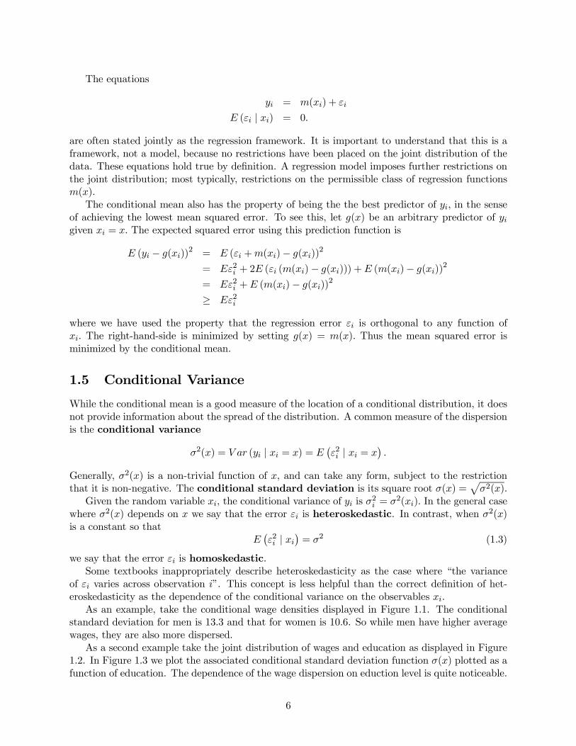
As a second example take the joint distribution of wages and education as displayed in Figure
1.2. In Figure 1.3 we plot the associated conditional standard deviation function σ(x) plotted as afunction of education. The dependence of the wage dispersion on eduction level is quite noticeable.
6
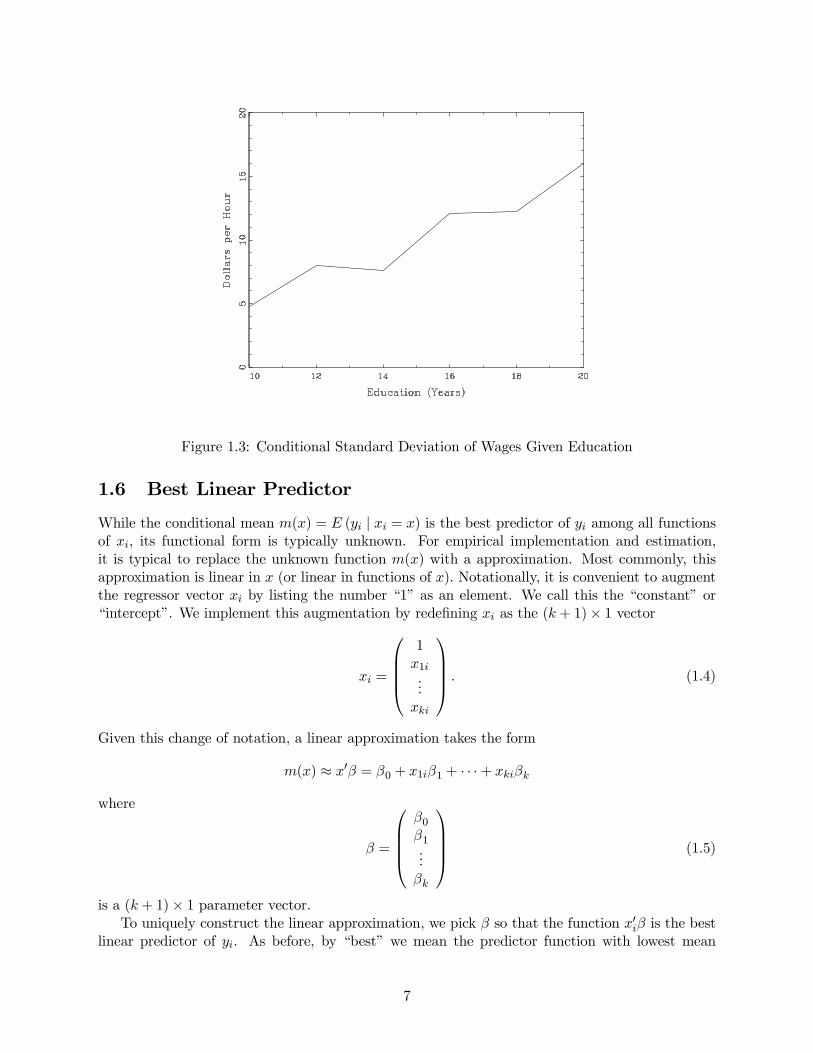
Figure 1.3: Conditional Standard Deviation of Wages Given Education
1.6 Best Linear Predictor
While the conditional mean m(x) = E (yi | xi = x) is the best predictor of yi among all functionsof xi, its functional form is typically unknown. For empirical implementation and estimation,
it is typical to replace the unknown function m(x) with a approximation. Most commonly, thisapproximation is linear in x (or linear in functions of x). Notationally, it is convenient to augmentthe regressor vector xi by listing the number “1” as an element. We call this the “constant” or
“intercept”. We implement this augmentation by redefining xi as the (k + 1)× 1 vector
xi =
⎛⎜⎜⎜⎝1x1i...
xki
⎞⎟⎟⎟⎠ . (1.4)
Given this change of notation, a linear approximation takes the form
m(x) ≈ x0β = β0 + x1iβ1 + · · ·+ xkiβk
where
β =
⎛⎜⎜⎜⎝β0β1...
βk
⎞⎟⎟⎟⎠ (1.5)
is a (k + 1)× 1 parameter vector.To uniquely construct the linear approximation, we pick β so that the function x0iβ is the best
linear predictor of yi. As before, by “best” we mean the predictor function with lowest mean
7
squared error. For any β ∈ Rk+1 a linear predictor for yi is x0iβ with expected squared prediction
error
S(β) = E¡yi − x0iβ
¢2= Ey2i − 2E
¡yix
0i
¢β + β0E
¡xix
0i
¢β.
which is quadratic in β. The best linear predictor is obtained by selecting β to minimize S(β).The first-order condition for minimization (from Appendix B.7) is
0 =∂
∂βS(β) = −2E (xiyi) + 2E
¡xix
0i
¢β.
Solving for β we find
β =¡E¡xix
0i
¢¢−1E (xiyi) . (1.6)
This vector exists and is unique as long as E (xix0i) is invertible, which we assume for now. Given
the definition of β in (1.6), x0iβ is the best linear predictor for yi.The error is
ei = yi − x0iβ. (1.7)
Notice that we use ei to denote the error from the linear prediction equation, to distinguish it from
the regression error εi. Rewriting, we obtain a decomposition of yi into linear predictor and error
yi = x0iβ + ei. (1.8)
This completes the definition of the linear projection model. We now summarize the as-
sumptions necessary for its derivation and list the implications in Theorem 1.6.1.
Assumption 1.6.1
1. xi contains an intercept;
2. Ey2i <∞;3. Ex0ixi <∞;4. Exix
0i is invertible.
Theorem 1.6.1 Under Assumption 1.6.1, (1.6) and (1.7) are well defined. Furthermore,
E (xiei) = 0. (1.9)
and
E (ei) = 0. (1.10)
Proof. Assumption 1.6.1.2 and 1.6.1.3 ensure that the moments in (1.6) are defined. Assump-
tion 1.6.1.4 guarantees that the solution β exits. Using the definitions (1.7) and (1.6)
E (xiei) = E¡xi¡yi − x0iβ
¢¢= E (xiyi)−E
¡xix
0i
¢ ¡E¡xix
0i
¢¢−1E (xiyi)
= 0.
8
Equation (1.10) follows from (1.9) and the assumption that xi contains an intercept. ¥
Since E (xiei) = 0 we say that xi and ei are orthogonal. This means that the equation
(1.8) can be alternatively interpreted as a projection decomposition. By definition, x0iβ is theprojection of yi on xi since the error ei is orthogonal with xi. Since ei is mean zero by (1.10), the
orthogonality restriction (1.9) implies that xi and ei are uncorrelated.
Recall from Theorem 1.4.1.4 that the regression error εi has the property E (xiεi) = 0. Thismeans that if the conditional mean is linear, so that m(x) = x0β, then the conditional mean andprojection coincide, and εi = ei. This is a special situation known as a linear regression model
yi = x0iβ + εi. It is special because in general the conditional mean function is nonlinear. While
the projection error ei is orthogonal to xi, i.e. E(xiei) = 0, it does not (in general) have a zeroconditional mean, i.e. E (ei | xi) 6= 0. This is due to the discrepancy between the linear projectionand the conditional mean.
The conditions listed in Assumption 1.6.1 are weak. The requirements of finite variances are
regularity conditions and are not considered important modelling assumptions. The critical
condition is that Exix0i is invertible, which we now discuss. Observe that for any non-zero α ∈
Rk+1, α0Exix0iα = E (α0xi)2 ≥ 0 so the matrix Exix0i is by construction positive semi-definite. It
is invertible if and only if it is positive definite, written Exix0i > 0, which requires that for all
non-zero α, α0Exix0iα = E (α0xi)2 > 0. Equivalently, there cannot exist a non-zero vector α suchthat α0xi = 0 identically. This occurs when redundant variables are included in xi. Assumption
1.6.1.4 excludes this troublesome case.
We have shown that under mild regularity conditions, for any pair (yi, xi) we can define a linearprojection equation (1.8) with the properties listed in Theorem 1.6.1. No additional assumptions
are required. However, it is important to not misinterpret the generality of this statement. The
linear equation (1.8) is defined by projection and the associated coefficient definition (1.6). In
contrast, in many economic models, the parameter β may be defined within the model. In this
case (1.6) may not hold and the implications of Theorem 1.6.1 may be false. These structural
models require alternative estimation methods, and are discussed in Chapter 7.
Returning to the joint distribution displayed in Figure 1.2, the dashed line is the linear pro-
jection of wages on eduction. In this example the linear projection is a close approximation to the
conditional mean. In other cases the two may be quite different. Figure 1.4 displays the relation-
ship3 between mean hourly wages and labor market experience. The solid line is the conditional
mean, and the straight dashed line is the linear projection. In this case the linear projection is not
a good approximation to the conditional mean. It over-predicts wages for young and old workers,
and under-predicts for the rest. Most importantly, it misses the strong downturn in expected
wages for those above 35 years work experience (equivalently, for those over 53 in age).
This defect in linear projection can be partially corrected through a careful selection of re-
gressors. In the example just presented, we can augment the regressor vector xi to include both
experience and experience2. A projection of wages on these two variables can perhaps be called
a quadratic projection, since the resulting function is quadratic in experience. Other than the
redefinition of the regressor vector, there are no changes in our methods or analysis. In Figure 1.4
we display as well this quadratic projection. In this example it is a much better approximation to
the conditional mean than the linear projection.
3Caucasian non-military male wage earners with 12 years of education.
9
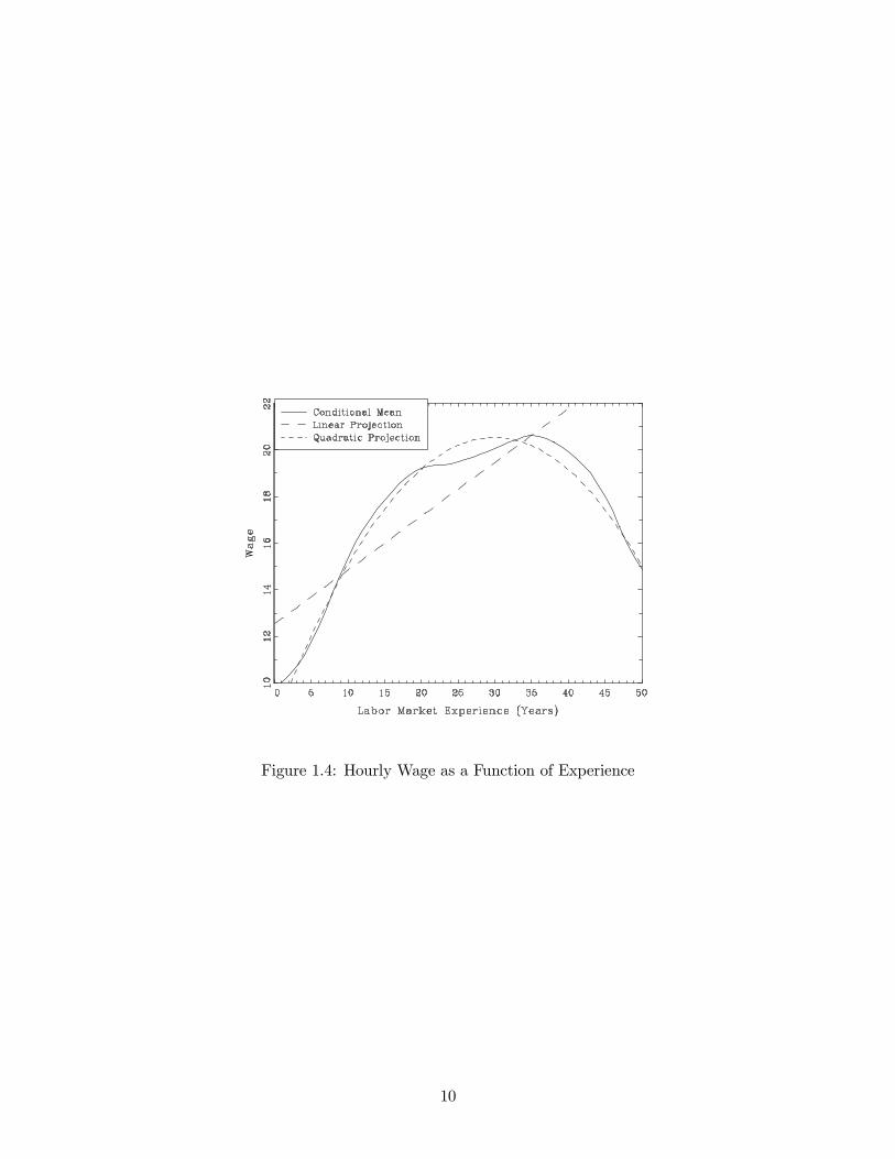
Figure 1.4: Hourly Wage as a Function of Experience
10
Chapter 2
Least Squares Estimation
This chapter explores estimation and inference in the linear projection model
yi = x0iβ + ei
E (xiei) = 0.
.
2.1 Estimation
Equation (1.6) writes the projection coefficient β as an explicit function of population moments
E (xiyi) and E (xix0i) . Their moment estimators are the sample moments
E (xiyi) =1
n
nXi=1
xiyi
E¡xix
0i
¢=
1
n
nXi=1
xix0i.
It follows that the moment estimator of β is (1.6) with the population moments replaced by the
sample moments:
β =
Ã1
n
nXi=1
xix0i
!−11
n
nXi=1
xiyi
=
ÃnXi=1
xix0i
!−1 nXi=1
xiyi. (2.1)
Another way to derive β is as follows. Observe that (1.9) can be written in the parametric
form
E¡xi¡yi − x0iβ
¢¢= 0. (2.2)
The function g(β) = E (xi (yi − x0iβ)) can be estimated by
g(β) =1
n
nXi=1
xi¡yi − x0iβ
¢11
and β is the value which sets this equal to zero:
0 =1
n
nXi=1
xi
³yi − x0iβ
´(2.3)
=1
n
nXi=1
xiyi − 1n
nXi=1
xix0iβ
whose solution is (2.1).
2.2 Least Squares
There is another classic motivation for the estimator (2.1). Define the sum-of-squared errors
(SSE) function
Sn(β) =nXi=1
¡yi − x0iβ
¢2.
TheOrdinary Least Squares (OLS) estimator is the value of β which minimizes Sn(β). Observethat we can write the latter as
Sn(β) =nXi=1
y2i − 2β0nXi=1
xiyi + β0nXi=1
xix0iβ.
Matrix calculus (see Appendix B.7) gives the first-order conditions for minimization:
0 =∂
∂βSn(β)
= −2nXi=1
xiyi + 2nXi=1
xix0iβ
whose solution is (2.1). Following convention we will call β the OLS estimator of β.
As a by-product of OLS estimation, we define the predicted value
yi = x0iβ
and the residual
ei = yi − yi
= yi − x0iβ.
Note that yi = yi + ei. It is important to understand the distinction between the error ei and the
residual ei. The error is unobservable, while the residual is a by-product of estimation. These two
variables are frequently mislabeled, which can cause confusion.
Equation (2.3) implies that
1
n
nXi=1
xiei = 0.
Since xi contains a constant, one implication is that
1
n
nXi=1
ei = 0.
12
Thus the residuals have a sample mean of zero and the sample correlation between the regressors
and the residual is zero. These are algebraic results, and hold true for all linear regression estimates.
The error variance σ2 = Ee2i is also a parameter of interest. It measures the variation in the
“unexplained” part of the regression. The method of moments estimator is the sample average
σ2 =1
n
nXi=1
e2i . (2.4)
An alternative estimator uses the formula
s2 =1
n− k − 1nXi=1
e2i . (2.5)
A justification for the latter choice will be provided in Section 3.4.
A measure of the explained variation relative to the total variation is the coefficient of de-
termination or R-squared.
R2 =
Pni=1(x
0iβ)
2Pni=1 (yi − y)2
= 1− σ2
σ2y
where
σ2y =1
n
nXi=1
(yi − y)2
is the sample variance of yi. The R2 is frequently mislabeled as a measure of “fit”. It is an
inappropriate label as the value of R2 does not aid in the interpretation of parameter estimates or
test statistics. Instead, it should be viewed as an estimator of the population parameter
ρ2 =V ar (x0iβ)V ar(yi)
= 1− σ2
σ2y
where σ2y = V ar(yi). An alternative estimator of ρ2 proposed by Theil called “R-bar-squared” is
R2= 1− (e
0e) / (n− k − 1)σ2y
= 1− s2
σ2y
where
σ2y =1
n− 1nXi=1
(yi − y)2 .
Theil’s estimator R2is an ratio of adjusted variance estimators, and therefore is expected to be a
better estimator of ρ2 than the unadjusted estimator R2.
2.3 Model in Matrix Notation
For some purposes, including computation, it is convenient to write the model and statistics in
matrix notation. We define
Y =
⎛⎜⎜⎜⎝y1y2...
yn
⎞⎟⎟⎟⎠ , X =
⎛⎜⎜⎜⎝x01x02...
x0n
⎞⎟⎟⎟⎠ , e =
⎛⎜⎜⎜⎝e1e2...
en
⎞⎟⎟⎟⎠ .
13
Observe that Y and e are n× 1 vectors, and X is an n× (k + 1) matrix.The linear equation (1.8) is a system of n equations, one for each observation. We can stack
these n equations together as
y1 = x01β + e1
y2 = x02β + e2...
yn = x0nβ + en.
or equivalently
Y = Xβ + e.
Sample sums can also be written in matrix notation. For example
nXi=1
xix0i = X 0X
nXi=1
xiyi = X 0Y.
Thus the estimator (2.1), residual vector, and sample error variance can be written as
β =¡X 0X
¢−1 ¡X 0Y
¢e = Y −Xβ
σ2 = n−1e0e.
Define the projection matrices
P = X¡X 0X
¢−1X 0
M = In − P.
where In is the n× n identity matrix. Then
Y = Xβ = X¡X 0X
¢−1X 0Y = PY
and
e = Y −Xβ = Y − PY = (In − P )Y =MY. (2.6)
Another way of writing this is
Y = (P +M)Y = PY +MY = Y + e.
This decomposition is orthogonal, that is
Y 0e = (PY )0 (MY ) = Y 0PMY = 0.
14
2.4 Residual Regression
Partition
X = [X1 X2]
and
β =
µβ1β2
¶.
Then the regression model can be rewritten as
Y = X1β1 +X2β2 + e. (2.7)
Observe that the OLS estimator of β = (β01, β02)0 can be obtained by regression of Y on X = [X1
X2]. OLS estimation can be written as
Y = X1β1 +X2β2 + e. (2.8)
Suppose that we are primarily interested in β2, not in β1, so are only interested in obtaining
the OLS sub-compontent β2. In this section we derive an alternative expression for β2 which does
not involve estimation of the full model.
Define
M1 = In −X1
¡X 01X1
¢−1X 01.
Recalling the definition M = I −X (X 0X)−1X 0, observe that X 01M = 0 and thus
M1M =M −X1¡X 01X1
¢−1X 01M =M
It follows that
M1e =M1Me =Me = e.
Using this result, if we premultiply (2.8) by M1 we obtain
M1Y = M1X1β1 +M1X2β2 +M1e
= M1X2β2 + e (2.9)
the second equality since M1X1 = 0. Premultiplying by X 02 and recalling that X
02e = 0, we obtain
X 02M1Y = X 0
2M1X2β2 +X 02e = X 0
2M1X2β2.
Solving,
β2 =¡X 02M1X2
¢−1 ¡X 02M1Y
¢an alternative expression for β1.
Now, define
X2 = M1X2 (2.10)
Y = M1Y, (2.11)
the least-squares residuals from the regression of X2 and Y, respectively, on the matrix X1 only.
Since the matrix M1 is idempotent, M1 =M1M1 and thus
β2 =¡X 02M1X2
¢−1 ¡X 02M1Y
¢=
¡X 02M1M1X2
¢−1 ¡X 02M1M1Y
¢=
³X 02X2
´−1 ³X 02Y´
15
This shows that β1 can be calculated by the OLS regression of Y on X2. This technique is called
residual regression.
Furthermore, using the definitions (2.10) and (2.11), expression (2.9) can be equivalently writ-
ten as
Y2 = X2β2 + e.
Since β2 is precisely the OLS coefficient from a regression of Y2 on X2, this shows that the residual
from this regression is e, numerically the same residual as from the joint regression (2.8). We have
proven the following theorem.
Theorem 2.4.1 (Frisch-Waugh-Lovell). In the model (2.7), the OLS estimator of β2 and the OLS
residuals e may be equivalently computed by either the OLS regression (2.8) or via the following
algorithm:
1. Regress Y on X1, obtain residuals Y ;
2. Regress X2 on X1, obtain residuals X2;
3. Regress Y on X2, obtain OLS estimates β2 and residuals e.
In some contexts, the FWL theorem can be used to speed computation, but in most cases there
is little computational advantage to using the two-step algorithm. Rather, the theorem’s primary
use is theoretical.
A common application of the FWL theorem, which you may have seen in an introductory
econometrics course, is the demeaning formula for regression. Partition X = [X1 X2] whereX1 = ι is a vector of ones, and X2 is the vector of observed regressors. In this case,
M1 = I − ι¡ι0ι¢−1
ι0.
Observe that
X2 = M1X2 = X2 − ι¡ι0ι¢−1
ι0X2= X2 −X2
and
Y = M1Y = Y − ι¡ι0ι¢−1
ι0Y= Y − Y ,
which are “demeaned”. The FWL theorem says that β2 is the OLS estimate from a regression of
Y on X2, or yi − y on x2i − x2 :
β2 =
ÃnXi=1
(x2i − x2) (x2i − x2)0!−1Ã nX
i=1
(x2i − x2) (yi − y)
!.
Thus the OLS estimator for the slope coefficients is a regression with demeaned data.
16
2.5 Efficiency
Is the OLS estimator efficient, in the sense of achieving the smallest possible mean-squared error
among feasible estimators? The answer was affirmatively provided by Chamberlain (1987).
Suppose that the joint distribution of (yi, xi) is discrete. That is, for finite r,
P¡yi = τ j , xi = ξj
¢= πj, j = 1, ..., r
for some constant vectors τ j , ξj, and πj . Assume that the τ j and ξj are known, but the πj are
unknown. (We know the values yi and xi can take, but we don’t know the probabilities.)
In this discrete setting, the moment condition (2.2) can be rewritten as
rXj=1
πjξj¡τ j − ξ0jβ
¢= 0. (2.12)
By the implicit function theorem, β is a function of (π1, ..., πr) .As the data are multinomial, the maximum likelihood estimator (MLE) is
πj =1
n
nXi=1
1 (yi = τ j) 1¡xi = ξj
¢for j = 1, ..., r, where 1 (·) is the indicator function. That is, πj is the percentage of the observationswhich fall in each category. The MLE βmle for β is then the function of (π1, ..., πr) which satisfiesthe analog of (2.12) with the πi replaced by the πi :
rXj=1
πjξj
³τ j − ξ0jβmle
´= 0.
Substituting in the expressions for πj ,
0 =rX
j=1
Ã1
n
nXi=1
1 (yi = τ j) 1¡xi = ξj
¢!ξj
³τ j − ξ0j βmle
´=
1
n
nXi=1
rXj=1
1 (yi = τ j) 1¡xi = ξj
¢ξj
³τ j − ξ0j βmle
´=
1
n
nXi=1
xi
³yi − x0iβmle
´But this is the same expression as (2.3), which means that βmle = βols. In other words, if the data
have a discrete distribution, the maximum likelihood estimator is identical to the OLS estimator.
Since this is a regular parametric model the MLE is asymptotically efficient, and thus so is the
OLS estimator.
Chamberlain (1987) extends this argument to the case of continuously-distributed data. He
observes that the above argument holds for all multinomial distributions, and any continuous
distribution can be arbitrarily well approximated by a multinomial distribution. He proves that
generically the OLS estimator (2.1) is an asymptotically efficient estimator for the parameter β
defined in (1.6) for the class of models satisfying Assumption 1.6.1.
17
2.6 Consistency
The OLS estimator β is a statistic, and thus has a statistical distribution. In general, this distrib-
ution is unknown. Asymptotic (large sample) methods approximate sampling distributions based
on the limiting experiment that the sample size n tends to infinity. A preliminary step in this
approach is the demonstration that estimators are consistent — that they converge in probability
to the true parameters as the sample size gets large.
Theorem 2.6.1 Under Assumption 1.6.1, as n→∞, β →p β, σ2 →p σ
2 and s2 →p σ2.
Proof. The following decomposition is quite useful.
β =
ÃnXi=1
xix0i
!−1 nXi=1
xiyi
=
ÃnXi=1
xix0i
!−1 nXi=1
xi¡x0iβ + ei
¢=
ÃnXi=1
xix0i
!−1Ã nXi=1
xix0i
!β +
ÃnXi=1
xix0i
!−1 nXi=1
xiei
= β +
ÃnXi=1
xix0i
!−1 nXi=1
xiei. (2.13)
This shows that after centering, the distribution of β is determined by the joint distribution of
(xi, ei) only.
We can now deduce the consistency of β. First, Assumption 1.6.1 and the WLLN (Theorem
D.2.1) imply that
1
n
nXi=1
xix0i →p E
¡xix
0i
¢= Q (2.14)
and1
n
nXi=1
xiei →p E (xiei) = 0. (2.15)
Using (2.13), we can write
β = β +
ÃnXi=1
xix0i
!−1 nXi=1
xiei
= β +
Ã1
n
nXi=1
xix0i
!−1Ã1
n
nXi=1
xiei
!
= β + g
Ã1
n
nXi=1
xix0i,1
n
nXi=1
xiei
!where g(A, b) = A−1b is a continuous function of A and b, at all values of the arguments such thatA−1 exist. Now by (2.14) and (2.15),Ã
1
n
nXi=1
xix0i,1
n
nXi=1
xiei
!→p (Q, 0) .
18
Assumption 1.6.1.4 implies that Q−1 exists and thus g(·, ·) is continuous at (Q, 0). Hence by thecontinuous mapping theorem (Theorem D.5.1),
g
Ã1
n
nXi=1
xix0i,1
n
nXi=1
xiei
!→p g (Q, 0) = Q−10 = 0
so
β = β + g
Ã1
n
nXi=1
xix0i,1
n
nXi=1
xiei
!→p β + 0 = 0.
We now examine σ2. Using (2.6),
nσ2 = e0MMe = e0Me = e0e− e0Pe. (2.16)
An application of the WLLN yields
1
n
nXi=1
e2i →p Ee2i = σ2
as n→∞, so combined with (2.14) and (2.15),
σ2 =1
n
nXi=1
e2i −1
n
nXi=1
eix0i
Ã1
n
nXi=1
xix0i
!−1Ã1
n
nXi=1
xiei
!→p σ
2 − 00Q−10 = σ2 (2.17)
so σ2 is consistent for σ2.
Finally, since n/(n− k)→ 1 as n→∞, it follows that
s2 =n
n− kσ2 →p σ
2.
2.7 Asymptotic Normality
We now establish the asymptotic distribution of β after normalization. We need a strengthening
of the moment conditions.
Assumption 2.7.1 In addition to Assumption 1.6.1, Ee4i <∞ and E |xi|4 <∞.
Now define
Ω = E¡xix
0ie2i
¢.
Assumption (2.7.1) guarantees that the elements of Ω are finite. To see this, by the Cauchy-Schwarzinequality (D.6),
E¯xix
0ie2i
¯ ≤ ³E ¯xix0i¯2´1/2 ¡E ¯e4i ¯¢1/2 = ³E |xi|4´1/2 ¡E ¯e4i ¯¢1/2 <∞. (2.18)
Thus xiei is iid with mean zero and has covariance matrix Ω. By the central limit theorem
(Theorem D.4.1),
1√n
nXi=1
xiei →d N (0,Ω) . (2.19)
19
Then using (2.13), (2.14), and (2.19),
√n³β − β
´=
Ã1
n
nXi=1
xix0i
!−1Ã1√n
nXi=1
xiei
!→d Q−1N (0,Ω)
= N¡0,Q−1ΩQ−1
¢.
Theorem 2.7.1 Under Assumption 2.7.1, as n→∞√n³β − β
´→d N (0, V )
where V = Q−1ΩQ−1.
As V is the variance of the asymptotic distribution of√n³β − β
´, V is often referred to as
the asymptotic covariance matrix of β. The form V = Q−1ΩQ−1 is called a sandwich form.There is a special case where Ω and V simplify. We say that ei is a Homoskedastic Projec-
tion Error when
Cov(xix0i, e
2i ) = 0. (2.20)
Condition (2.20) holds, for example, when xi and ei are independent, but this is not a necessary
condition. Under (2.20) the asymptotic variance formulas simplify as
Ω = E¡xix
0i
¢E¡e2i¢= Qσ2 (2.21)
V = Q−1ΩQ−1 = Q−1σ2 ≡ V 0 (2.22)
In (2.22) we define V 0 = Q−1σ2 whether (2.20) is true or false. When (2.20) is true then V = V 0,
otherwise V 6= V 0. We call V 0 the homoskedastic covariance matrix.
2.8 Covariance Matrix Estimation
Let
Q =1
n
nXi=1
xix0i =
1
nX 0X
be the method of moments estimator for Q. The homoskedastic covariance matrix V 0 = Q−1σ2 istypically estimated by
V 0 = Q−1s2. (2.23)
Since Q →p Q and s2 →p σ2 (see (2.14) and Theorem 2.6.1) it is clear that V 0 →p V 0. The
estimator σ2 may also be substituted for s2 in (2.23) without changing this result.
To estimate V = Q−1ΩQ−1, we need an estimate of Ω = E¡xix
0ie2i
¢. The MME estimator is
Ω =1
n
nXi=1
xix0ie2i
20
where ei are the OLS residuals. A useful computational formula is to define ui = xiei and the
n× (k + 1) matrix
u =
⎛⎜⎜⎜⎝u01u02...
u0n
⎞⎟⎟⎟⎠ .
Then
Ω =1
nu0u
V = n¡X 0X
¢−1 ¡u0u¢ ¡X 0X
¢−1This estimator was introduced to the econometrics literature by White (1980).
The estimator V 0 was the dominate covariance estimator used before 1980, and was still the
standard choice for much empirical work done in the early 1980s. The methods switched during
the late 1980s and early 1990s, so that by the late 1990s White estimate V emerged as the standard
covariance matrix estimator. When reading and reporting applied work, it is important to pay
attention to the distinction between V 0 and V , as it is not always clear which has been computed.
When V is used rather than the traditional choice V 0, many authors will state that “their standard
errors have been corrected for heteroskedasticity”, or that they use a “heteroskedasticity-robust
covariance matrix estimator”, or that they use the “White formula”, the “Eicker-White formula”,
the “Huber formula”, the “Huber-White formula” or the “GMM covariance matrix”. In most
cases, these all mean the same thing.
We now show Ω→p Ω, from which it follows that V →p V as n→∞. Expanding the quadratic
e2i =³yi − x0iβ
´2=
³ei − x0i
³β − β
´´2= e2i − 2
³β − β
´0xiei +
³β − β
´0xix
0i
³β − β
´.
Hence
Ω =1
n
nXi=1
xix0ie2i
=1
n
nXi=1
xix0ie2i −
2
n
nXi=1
xix0i
³β − β
´0xiei +
1
n
nXi=1
xix0i
³β − β
´0xix
0i
³β − β
´. (2.24)
We now examine the each sum on the right-hand-side of (2.24) in turn. First, (2.18) and the
WLLN (Theorem D.2.1) show that
1
n
nXi=1
xix0ie2i →p E
¡xix
0ie2i
¢= Ω.
Second, by Holder’s inequality (D.5)
E³|xi|3 |ei|
´≤³E |xi|4
´3/4 ¡E¯e4i¯¢1/4
<∞,
21
so by the WLLN
1
n
nXi=1
|xi|3 |ei|→p E³|xi|3 |ei|
´,
and thus since¯β − β
¯→p 0,¯
¯ 1nnXi=1
xix0i
³β − β
´0xiei
¯¯ ≤ ¯β − β
¯ Ã1n
nXi=1
|xi|3 |ei|!→p 0.
Third, by the WLLN
1
n
nXi=1
|xi|4 →p E |xi|4 ,
so ¯¯ 1n
nXi=1
xix0i
³β − β
´0xixi
³β − β
´¯¯ ≤ ¯β − β¯2 1n
nXi=1
|xi|4 →p 0.
Together, these establish consistency.
Theorem 2.8.1 As n→∞, Ω→p Ω.
The variance estimator V is an estimate of the variance of the asymptotic distribution of β.
A more easily interpretable measure of spread is its square root — the standard deviation. This
motivates the definition of a standard error.
Definition 2.8.1 A standard error s(β) for an estimator β is an estimate of the standard
deviation of the distribution of β.
When β is scalar, and V is an estimator of the variance of√n³β − β
´, we set s(β) = n−1/2
pV .
When β is a vector, we focus on individual elements of β one-at-a-time, vis., βj, j = 0, 1, ..., k.Thus
s(βj) = n−1/2qVjj.
Generically, standard errors are not unique, as there may be more than one estimator of the
variance of the estimator. It is therefore important to understand what formula and method is
used by an author when studying their work. It is also important to understand that a particular
standard error may be relevant under one set of model assumptions, but not under another set of
assumptions, just as any other estimator.
From a computational standpoint, the standard method to calculate the standard errors is to
first calculate n−1V , then take the diagonal elements, and then the square roots.
2.9 Multicollinearity
If rank(X 0X) < k + 1, then β is not defined. This is called strict multicollinearity. This
happens when the columns of X are linearly dependent, i.e., there is some α such that Xα = 0.Most commonly, this arises when sets of regressors are included which are identically related.
For example, if X includes both the logs of two prices and the log of the relative prices log(p1),log(p2) and log(p1/p2). When this happens, the applied researcher quickly discovers the error as
22
the statistical software will be unable to construct (X 0X)−1. Since the error is discovered quickly,this is rarely a problem for applied econometric practice.
The more relevant issue is near multicollinearity, which is often called “multicollinearity”
for brevity. This is the situation when the X 0X matrix is near singular, when the columns of X are
close to linearly dependent. This definition is not precise, because we have not said what it means
for a matrix to be “near singular”. This is one difficulty with the definition and interpretation of
multicollinearity.
One implication of near singularity of matrices is that the numerical reliability of the calcula-
tions is reduced. It is possible that the reported calculations will be in error due to floating-point
calculation difficulties.
More relevantly in practice, an implication of near multicollinearity is that estimation precision
of individual coefficients will be poor. We can see this most simply in a model with two regressors
and no intercept:
yi = x1iβ1 + x2iβ2 + ei,
under (2.20) and
E
µx21i x1ix2i
x1ix2i x22i
¶=
µ1 ρ
ρ 1
¶In this case the asymptotic covariance matrix V is
σ2µ1 ρ
ρ 1
¶−1= σ2
¡1− ρ2
¢−1µ 1 −ρ−ρ 1
¶.
The correlation ρ indexes collinearity, since as ρ approaches 1 the matrix becomes singular. We can
see the effect of collinearity on precision by examining the asymptotic variance of either coefficient
estimate, which is σ2¡1− ρ2
¢−1. As ρ approaches 1, the variance rises quickly to infinity. Thus the
more “collinear” are the regressors, the worse the precision of the individual coefficient estimates.
Basically, what is happening is that when the regressors are highly dependent, it is statistically
difficult to disentangle the impact of β1 from that of β2. The precision of individual estimates are
reduced.
Is there a simple solution? Basically, No. Fortunately, multicollinearity does not lead to errors
in inference. The asymptotic distribution is still valid. Regression estimates are asymptotically
normal, and estimated standard errors are consistent for the asymptotic variance. Consequently,
reported confidence intervals are not inherently misleading. They will be large, correctly indicating
the inherent uncertainty about the true parameter value.
2.10 Omitted Variables
Let the regressors be partitioned as
xi =
µx1ix2i
¶.
Suppose we are interested in the coefficient on x1i alone in the regression of yi on the full set xi.
We can write the model as
yi = x01iβ1 + x02iβ2 + ei (2.25)
E (xiei) = 0
where the parameter of interest is β1.
23
Now suppose that instead of estimating equation (2.25) by least-squares, we regress yi on x1ionly. This is estimation of the equation
yi = x01iγ1 + ui (2.26)
E (x1iui) = 0
Notice that we have written the coefficient on x1i as γ1 rather than β1, and the error as ui rather
than ei. This is because the model being estimated is different than (2.25). Goldberger calls (2.25)
the long regression and (2.26) the short regression to emphasize the distinction.
Typically, β1 6= γ1, except in special cases. To see this, we calculate
γ1 =¡E¡x1ix
01i
¢¢−1E (x1iyi)
=¡E¡x1ix
01i
¢¢−1E¡x1i¡x01iβ1 + x02iβ2 + ei
¢¢= β1 +
¡E¡x1ix
01i
¢¢−1E¡x1ix
02i
¢β2
= β1 + Γβ2
where
Γ =¡E¡x1ix
01i
¢¢−1E¡x1ix
02i
¢is the coefficient from a regression of x2i on x1i.
Observe that γ1 6= β1 unless Γ = 0 or β2 = 0. Thus the short and long regressions have thesame coefficient on x1i only under one of two conditions. First, the regression of x2i on x1i yields a
set of zero coefficients (they are uncorrelated), or second, the coefficient on x2i in (2.25) is zero. In
general, least-squares estimation of (2.26) produces a consistent estimate of γ1 = β1 + Γβ2 ratherthan β1. The difference Γβ2 is known as omitted variable bias. It is the consequence of omissionof a relevant correlated variable.
To avoid omitted variables bias the standard advice is to include potentially relevant variables
in the estimated model. By construction, the general model will be free of the omitted variables
problem. Typically there are limits, as many desired variables are not available in a given dataset.
In this case, the possibility of omitted variables bias should be acknowledged and discussed in the
course of an empirical investigation.
2.11 Irrelevant Variables
In the model
yi = x01iβ1 + x02iβ2 + ei
E (xiei) = 0,
x2i is “irrelevant” if β1 is the parameter of interest and β2 = 0. One estimator of β1 is to regressyi on x1i alone, β1 = (X 0
1X1)−1 (X 0
1Y ) . Another is to regress yi on x1i and x2i jointly, yielding
(β1, β2). Under which conditions is β1 or β1 superior?First, it is easy to see that both are consistent for β1. So in comparison with the problem of
omitted variables, we see that the presence (or absence) of irrelevant variables is relatively less
important.
Second, we can consider the relative efficiency of β1 versus β1.We focus on the homoskedastic
case (2.20) since it is hard to make comparisons in the general case. In this case
limn→∞nV ar( β1) =
¡Ex1ix
01i
¢−1σ2 = Q−111 σ
2,
24
say, and
limn→∞nV ar(β1) =
¡Ex1ix
01i −Ex1ix
02i
¡Ex2ix
02i
¢Ex2ix
01i
¢−1σ2 =
¡Q11 −Q12Q
−122 Q21
¢−1σ2,
say. If Q12 = 0 (so the variables are orthogonal) then these two variance matrices equal, andthe two estimators have equal asymptotic efficiency. Otherwise, since Q12Q
−122 Q21 > 0, then
Q11 > Q11 −Q12Q−122 Q21, and consequently
Q−111 σ2 <
¡Q11 −Q12Q
−122 Q21
¢−1σ2.
This means that β1 has a lower asymptotic variance matrix than β1.We conclude that the inclusion
of irrelevant variables reduces estimation efficiency if these variables are correlated with the relevant
variables.
2.12 Functions of Parameters
Sometimes we are interested in some function of the parameter vector. Let h : Rk+1 → Rq, and
θ = h(β).
The estimate of θ is
θ = h(β).
What is an appropriate standard error for θ? Assume that h(β) is differentiable at the truevalue of β. By a first-order Taylor series approximation:
h(β) ' h(β) +H 0β
³β − β
´.
where
Hβ =∂
∂βh(β) (k + 1)× q.
Thus
√n³θ − θ
´=√n³h(β)− h(β)
´' H 0
β
√n³β − β
´→d H 0
βN(0, V )
= N(0, Vθ). (2.27)
where
Vθ = H 0βV Hβ.
If V is the estimated covariance matrix for β, then the natural estimate for the variance of θ is
Vθ = H 0βV Hβ
where
Hβ =∂
∂βh(β).
25
In many cases, the function h(β) is linear:
h(β) = R0β
for some (k + 1)× q matrix R. In this case, Hβ = R and Hβ = R, so Vθ = R0V R.For example, if R is a “selector matrix”
R =
µI
0
¶so that if β = (β1, β2), then θ = R0β = β1 and
Vθ =¡I 0
¢V
µI
0
¶= V11,
the upper-left block of V .
When q = 1 (so h(β) is real-valued), the standard error for θ is the square root of n−1Vθ, thatis, s(θ) = n−1/2
qH 0β V Hβ .
2.13 t tests
Let θ = h(β) : Rk+1 → R be any parameter of interest, θ its estimate and s(θ) its asymptoticstandard error. Consider the studentized statistic
tn(θ) =θ − θ
s(θ). (2.28)
Theorem 2.13.1 tn(θ)→d N(0, 1)
Proof. By (2.27)
tn(θ) =θ − θ
s(θ)
=
√n³θ − θ
´qVθ
→d
N(0, Vθ)√Vθ
= N(0, 1).
Thus the asymptotic distribution of the t-ratio tn(θ) is the standard normal. Since the standardnormal distribution does not depend on the parameters, we say that tn(θ) is asymptoticallypivotal. In special cases (such as the normal regression model, see Section X), the statistic tn has
an exact t distribution, and is therefore exactly free of unknowns. In this case, we say that tn is an
exactly pivotal statistic. In general, however, pivotal statistics are unavailable and so we must
rely on asymptotically pivotal statistics.
A simple null and composite hypothesis takes the form
H0 : θ = θ0
H1 : θ 6= θ0
26
where θ0 is some pre-specified value, and θ = h(β) is some function of the parameter vector. (Forexample, θ could be a single element of β).
The standard test for H0 against H1 is the t-statistic (or studentized statistic)
tn = tn(θ0) =θ − θ0
s(θ).
Under H0, tn →d N(0, 1). Let zα/2 is the upper α/2 quantile of the standard normal distribution.That is, if Z ∼ N(0, 1), then P (Z > zα/2) = α/2 and P (|Z| > zα/2) = α. For example, z.025 = 1.96and z.05 = 1.645. A test of asymptotic significance α rejects H0 if |tn| > zα/2. Otherwise the test
does not reject, or “accepts” H0. This is because
P (reject H0 | H0) = P¡|tn| > zα/2 | θ = θ0
¢→ P
¡|Z| > zα/2¢= α.
The rejection/acceptance dichotomy is associate with the Neyman-Pearson approach to hypothesis
testing.
An alternative approach, associate with Fisher, is to report an asymptotic p-value. The as-
ymptotic p-value for the above statistic is constructed as follows. Define the tail probability, or
asymptotic p-value function
p(t) = P (|Z| > |t|) = 2 (1−Φ(|t|)) .Then the asymptotic p-value of the statistic tn is
pn = p(tn).
If the p-value pn is small (close to zero) then the evidence against H0 is strong. In a sense,
p-values and hypothesis tests are equivalent since pn < α if and only if |tn| > zα/2. Thus an
equivalent statement of a Neyman-Pearson test is to reject at the α% level if and only if pn < α.
The p-value is more general, however, in that the reader is allowed to pick the level of significance
α, in contrast to Neyman-Pearson rejection/acceptance reporting where the researcher picks the
level.
Another helpful observation is that the p-value function has simply made a unit-free transfor-
mation of the test statistic. That is, under H0, pn →d U [0, 1], so the “unusualness” of the teststatistic can be compared to the easy-to-understand uniform distribution, regardless of the com-
plication of the distribution of the original test statistic. To see this fact, note that the asymptotic
distribution of |tn| is F (x) = 1− p(x). Thus
P (1− pn ≤ u) = P (1− p(tn) ≤ u)
= P (F (tn) ≤ u)
= P¡|tn| ≤ F−1(u)
¢→ F
¡F−1(u)
¢= u,
establishing that 1− pn →d U [0, 1], from which it follows that pn →d U [0, 1].
2.14 Confidence Intervals
A confidence interval Cn is an interval estimate of θ, and is a function of the data and hence is
random. It is designed to cover θ with high probability. Either θ ∈ Cn or θ /∈ Cn. The coverage
probability is P (θ ∈ Cn).
27
We typically cannot calculate the exact coverage probability P (θ ∈ Cn). However we often cancalculate the asymptotic coverage probability limn→∞ P (θ ∈ Cn). We say that Cn has asymptotic
(1− α)% coverage for θ if P (θ ∈ Cn)→ 1− α as n→∞.
A good method for construction of a confidence interval is the collection of parameter values
which are not rejected by a statistical test. The t-test of the previous setion rejects H0 : θ0 = θ if
|tn(θ)| > zα/2 where tn(θ) is the t-statistic (2.28) and zα/2 is the upper α/2 quantile of the standardnormal distribution. A confidence interval is then constructed as the values of θ for which this test
does not reject:
Cn =©θ : |tn(θ)| ≤ zα/2
ª=
(θ : zα/2 ≤
θ − θ
s(θ)≤ zα/2
)=
hθ − zα/2s(θ), θ + zα/2s(θ)
i. (2.29)
While there is no hard-and-fast guideline for choosing the coverage probability 1 − α, the
most common professional choice is 95%, or α = .05. This corresponds to selecting the confidence
intervalhθ ± 1.96s(θ)
i≈hθ ± 2s(θ)
i. Thus values of θ within two standard errors of the estimated
θ are considered “reasonable” candidates for the true value θ, and values of θ outside two standard
errors of the estimated θ are considered unlikely or unreasonable candidates for the true value.
The interval has been constructed so that as n→∞,
P (θ ∈ Cn) = P¡|tn(θ)| ≤ zα/2
¢→ P¡|Z| ≤ zα/2
¢= 1− α.
and Cn is an asymptotic (1− α)% confidence interval.
2.15 Wald Tests
Sometimes θ = h(β) is a q×1 vector, and it is desired to test the joint restrictions simultaneously.In this case the t-statistic approach does not work. We have the null and alternative
H0 : θ = θ0
H1 : θ 6= θ0.
The natural estimate of θ is θ = h(β) and has asymptotic covariance matrix estimate
Vθ = H 0βV Hβ
where
Hβ =∂
∂βh(β).
The Wald statistic for H0 against H1 is
Wn = n³θ − θ0
´0V −1θ
³θ − θ0
´= n
³h(β)− θ0
´0 ³H 0βV Hβ
´−1 ³h(β)− θ0
´. (2.30)
28
When h is a linear function of β, h(β) = R0β, then the Wald statistic takes the form
Wn = n³R0β − θ0
´0 ³R0V R
´−1 ³R0β − θ0
´.
The delta method (2.27) showed that√n³θ − θ
´→d Z ∼ N(0, Vθ), and Theorem 2.8.1 showed
that V →p V. Furthermore, Hβ(β) is a continuous function of β, so by the continuous mapping
theorem, Hβ(β)→p Hβ . Thus Vθ = H 0βV Hβ →p H
0βVHβ = Vθ > 0 if Hβ has full rank q. Hence
Wn = n³θ − θ0
´0V −1θ
³θ − θ0
´→d Z
0V −1θ Z = χ2q,
by Theorem C.8.1. We have established:
Theorem 2.15.1 Under H0 and Assumption 2.7.1, if rank(Hβ) = q, then Wn →d χ2q, a chi-
square random variable with q degrees of freedom.
An asymptotic Wald test rejects H0 in favor of H1 if Wn exceeds χ2q(α), the upper-α quantile
of the χ2q distribution. For example, χ21(.05) = 3.84 = z2.025. The Wald test fails to reject if Wn is
less than χ2q(α). The asymptotic p-value forWn is pn = p(Wn), where p(x) = P¡χ2q ≥ x
¢is the tail
probability function of the χ2q distribution. As before, the test rejects at the α% level iff pn < α,
and pn is asymptotically U [0, 1] under H0.
2.16 F Tests
Take the linear model
Y = X1β1 +X2β2 + e
where X1 is n× k1 and X2 is n× k2 and k + 1 = k1 + k2. The null hypothesis is
H0 : β2 = 0.
In this case, θ = β2, and there are q = k2 restrictions. Also h(β) = R0β is linear with R =
µ0I
¶a selector matrix. We know that the Wald statistic takes the form
Wn = nθ0V −1θ θ
= nβ02
³R0V R
´−1β2.
What we will show in this section is that if V is replaced with V 0 = σ2¡n−1X 0X
¢−1, the covariance
matrix estimator valid under homoskedasticity, then the Wald statistic can be written in the form
Wn = n
µσ2 − σ2
σ2
¶(2.31)
where
σ2 =1
ne0e, e = Y −X1β1, β1 =
¡X 01X1
¢−1X 01Y
29
are from OLS of Y on X1, and
σ2 =1
ne0e, e = Y −Xβ, β =
¡X 0X
¢−1X 0Y
are from OLS of Y on X = (X1,X2).The elegant feature about (2.31) is that it is directly computable from the standard output
from two simple OLS regressions, as the sum of square errors is a typical output from statistical
packages. This statistic is typically reported as an “F-statistic” which is defined as
F =n− k − 1
n
Wn
k2=
¡σ2 − σ2
¢/k2
σ2/(n− k − 1) .
While it should be emphasized that equality (2.31) only holds if V 0 = σ2¡n−1X 0X
¢−1, still this
formula often finds good use in reading applied papers. Because of this connection we call (2.31)
the F form of the Wald statistic.
We now derive expression (2.31). First, note that partitioned matrix inversion (B.1)
R0¡X 0X
¢−1R = R0
µX 01X1 X 0
1X2X 02X1 X 0
2X2
¶−1R =
¡X 02M1X2
¢−1where M1 = I −X1(X 0
1X1)−1X 0
1. Thus³R0V 0R
´−1= σ−2n−1
³R0¡X 0X
¢−1R´−1
= σ−2n−1¡X 02M1X2
¢and
Wn = nβ02
³R0V 0R
´−1β2
=β02 (X
02M1X2) β2σ2
.
To simplify this expression further, note that if we regress Y on X1 alone, the residual is
e = M1Y. Now consider the residual regression of e on X2 = M1X2. By the FWL theorem,
e = X2β2 + e and X 02e = 0. Thus
e0e =³X2β2 + e
´0 ³X2β2 + e
´= β
02X
02X2β2 + e0e
= β02X
02M1X2β2 + e0e,
or alternatively,
β02X
02M1X2β2 = e0e− e0e.
Also, since
σ2 = n−1e0e
we conclude that
Wn = n
µe0e− e0e
e0e
¶= n
µσ2 − σ2
σ2
¶,
as claimed.
30
In many statistical packages, when an OLS regression is reported, an “F statistic” is reported.
This is
F =
¡σ2y − σ2
¢/k
σ2/(n− k − 1) .
where
σ2y =1
n(y − y)0 (y − y)
is the sample variance of yi, equivalently the residual variance from an intercept-only model. This
special F statistic is testing the hypothesis that all slope coefficients (other than the intercept) are
zero. This was a popular statistic in the early days of econometric reporting, when sample sizes
were very small and researchers wanted to know if there was “any explanatory power” to their
regression. This is rarely an issue today, as sample sizes are typically sufficiently large that this F
statistic is highly “significant”. While there are special cases where this F statistic is useful, these
cases are atypical.
2.17 Problems with Tests of NonLinear Hypotheses
While the t and Wald tests work well when the hypothesis is a linear restriction on β, they can
work quite poorly when the restrictions are nonlinear. This can be seen by a simple example
introduced by Lafontaine and White (1986). Take the model
yi = β + ei
ei ∼ N(0, σ2)
and consider the hypothesis
H0 : β = 1.
Let β and σ2 be the sample mean and variance of yi. Then the standard Wald test for H0 is
Wn = n
³β − 1
´2σ2
.
Now notice that H0 is equivalent to the hypothesis
H0(s) : βs = 1
for any positive integer s. Letting h(β) = βs, and noting Hβ = sβs−1, we find that the standardWald test for H0(s) is
Wn(s) = n
³βs − 1
´2σ2s2β
2s−2 .
While the hypothesis βs = 1 is unaffected by the choice of s, the statistic Wn(s) varies with s.
This is an unfortunate feature of the Wald statistic.
To demonstrate this effect, we have plotted in Figure 2.1 the Wald statisticWn(s) as a functionof s, setting n/σ2 = 10. The increasing solid line is for the case β = 0.8. The decreasing dashedline is for the case β = 1.7. It is easy to see that in each case there are values of s for which thetest statistic is significant relative to asymptotic critical values, while there are other values of s
31
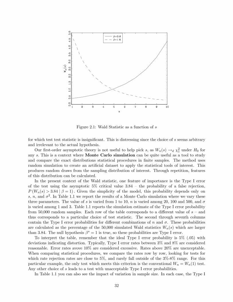
Figure 2.1: Wald Statistic as a function of s
for which test test statistic is insignificant. This is distressing since the choice of s seems arbitrary
and irrelevant to the actual hypothesis.
Our first-order asymptotic theory is not useful to help pick s, as Wn(s) →d χ21 under H0 for
any s. This is a context where Monte Carlo simulation can be quite useful as a tool to study
and compare the exact distributions statistical procedures in finite samples. The method uses
random simulation to create an artificial dataset to apply the statistical tools of interest. This
produces random draws from the sampling distribution of interest. Through repetition, features
of this distribution can be calculated.
In the present context of the Wald statistic, one feature of importance is the Type I error
of the test using the asymptotic 5% critical value 3.84 — the probability of a false rejection,
P (Wn(s) > 3.84 | β = 1) . Given the simplicity of the model, this probability depends only ons, n, and σ2. In Table 1.1 we report the results of a Monte Carlo simulation where we vary these
three parameters. The value of s is varied from 1 to 10, n is varied among 20, 100 and 500, and σ
is varied among 1 and 3. Table 1.1 reports the simulation estimate of the Type I error probability
from 50,000 random samples. Each row of the table corresponds to a different value of s — and
thus corresponds to a particular choice of test statistic. The second through seventh columns
contain the Type I error probabilities for different combinations of n and σ. These probabilities
are calculated as the percentage of the 50,000 simulated Wald statistics Wn(s) which are largerthan 3.84. The null hypothesis βs = 1 is true, so these probabilities are Type I error.
To interpret the table, remember that the ideal Type I error probability is 5% (.05) with
deviations indicating distortion. Typically, Type I error rates between 3% and 8% are considered
reasonable. Error rates avove 10% are considered excessive. Rates above 20% are unexceptable.
When comparing statistical procedures, we compare the rates row by row, looking for tests for
which rate rejection rates are close to 5%, and rarely fall outside of the 3%-8% range. For this
particular example, the only test which meets this criterion is the conventional Wn =Wn(1) test.Any other choice of s leads to a test with unacceptable Type I error probabilities.
In Table 1.1 you can also see the impact of variation in sample size. In each case, the Type I
32
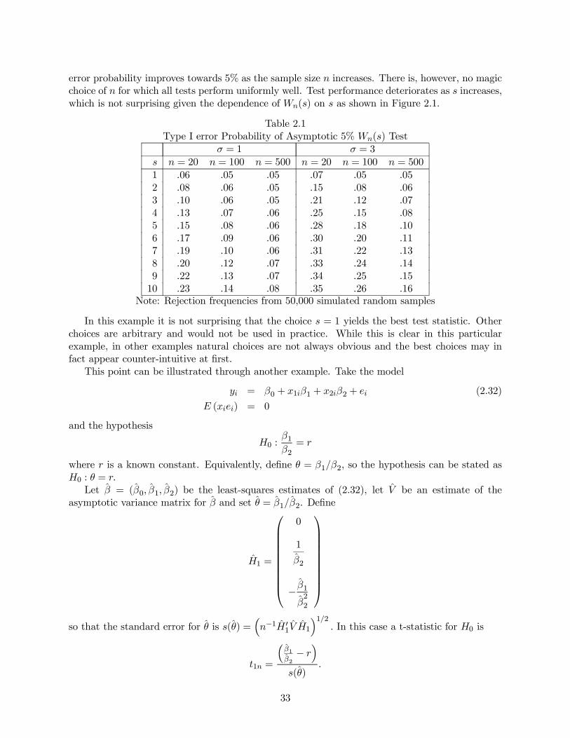
error probability improves towards 5% as the sample size n increases. There is, however, no magic
choice of n for which all tests perform uniformly well. Test performance deteriorates as s increases,
which is not surprising given the dependence of Wn(s) on s as shown in Figure 2.1.
Table 2.1
Type I error Probability of Asymptotic 5% Wn(s) Testσ = 1 σ = 3
s n = 20 n = 100 n = 500 n = 20 n = 100 n = 500
1 .06 .05 .05 .07 .05 .05
2 .08 .06 .05 .15 .08 .06
3 .10 .06 .05 .21 .12 .07
4 .13 .07 .06 .25 .15 .08
5 .15 .08 .06 .28 .18 .10
6 .17 .09 .06 .30 .20 .11
7 .19 .10 .06 .31 .22 .13
8 .20 .12 .07 .33 .24 .14
9 .22 .13 .07 .34 .25 .15
10 .23 .14 .08 .35 .26 .16
Note: Rejection frequencies from 50,000 simulated random samples
In this example it is not surprising that the choice s = 1 yields the best test statistic. Otherchoices are arbitrary and would not be used in practice. While this is clear in this particular
example, in other examples natural choices are not always obvious and the best choices may in
fact appear counter-intuitive at first.
This point can be illustrated through another example. Take the model
yi = β0 + x1iβ1 + x2iβ2 + ei (2.32)
E (xiei) = 0
and the hypothesis
H0 :β1β2= r
where r is a known constant. Equivalently, define θ = β1/β2, so the hypothesis can be stated as
H0 : θ = r.
Let β = (β0, β1, β2) be the least-squares estimates of (2.32), let V be an estimate of the
asymptotic variance matrix for β and set θ = β1/β2. Define
H1 =
⎛⎜⎜⎜⎜⎜⎜⎜⎜⎜⎝
0
1
β2
− β1β2
2
⎞⎟⎟⎟⎟⎟⎟⎟⎟⎟⎠so that the standard error for θ is s(θ) =
³n−1H 0
1V H1
´1/2. In this case a t-statistic for H0 is
t1n =
³β1β2− r´
s(θ).
33
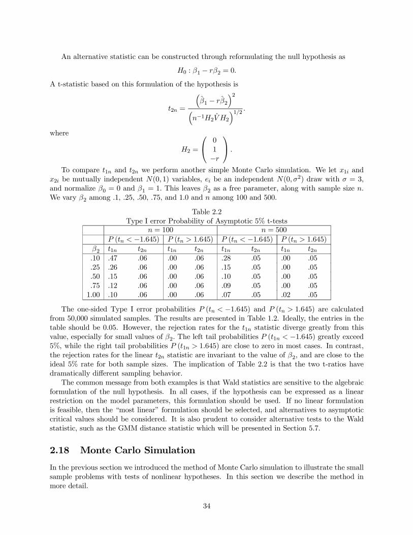
An alternative statistic can be constructed through reformulating the null hypothesis as
H0 : β1 − rβ2 = 0.
A t-statistic based on this formulation of the hypothesis is
t2n =
³β1 − rβ2
´2³n−1H2V H2
´1/2 .where
H2 =
⎛⎝ 01−r
⎞⎠ .
To compare t1n and t2n we perform another simple Monte Carlo simulation. We let x1i and
x2i be mutually independent N(0, 1) variables, ei be an independent N(0, σ2) draw with σ = 3,
and normalize β0 = 0 and β1 = 1. This leaves β2 as a free parameter, along with sample size n.We vary β2 among .1, .25, .50, .75, and 1.0 and n among 100 and 500.
Table 2.2
Type I error Probability of Asymptotic 5% t-tests
n = 100 n = 500
P (tn < −1.645) P (tn > 1.645) P (tn < −1.645) P (tn > 1.645)
β2 t1n t2n t1n t2n t1n t2n t1n t2n.10 .47 .06 .00 .06 .28 .05 .00 .05
.25 .26 .06 .00 .06 .15 .05 .00 .05
.50 .15 .06 .00 .06 .10 .05 .00 .05
.75 .12 .06 .00 .06 .09 .05 .00 .05
1.00 .10 .06 .00 .06 .07 .05 .02 .05
The one-sided Type I error probabilities P (tn < −1.645) and P (tn > 1.645) are calculatedfrom 50,000 simulated samples. The results are presented in Table 1.2. Ideally, the entries in the
table should be 0.05. However, the rejection rates for the t1n statistic diverge greatly from this
value, especially for small values of β2. The left tail probabilities P (t1n < −1.645) greatly exceed5%, while the right tail probabilities P (t1n > 1.645) are close to zero in most cases. In contrast,the rejection rates for the linear t2n statistic are invariant to the value of β2, and are close to the
ideal 5% rate for both sample sizes. The implication of Table 2.2 is that the two t-ratios have
dramatically different sampling behavior.
The common message from both examples is that Wald statistics are sensitive to the algebraic
formulation of the null hypothesis. In all cases, if the hypothesis can be expressed as a linear
restriction on the model parameters, this formulation should be used. If no linear formulation
is feasible, then the “most linear” formulation should be selected, and alternatives to asymptotic
critical values should be considered. It is also prudent to consider alternative tests to the Wald
statistic, such as the GMM distance statistic which will be presented in Section 5.7.
2.18 Monte Carlo Simulation
In the previous section we introduced the method of Monte Carlo simulation to illustrate the small
sample problems with tests of nonlinear hypotheses. In this section we describe the method in
more detail.
34
Recall, our data consist of observations (yi, xi) which are random draws from a population
distribution F. Let θ be a parameter and let Tn = Tn(y1, x1..., yn, xn, θ) be a statistic of interest,for example an estimator θ or a t-statistic (θ − θ)/s(θ). The exact distribution of Tn is
Gn(x, F ) = P (Tn ≤ x | F ) .
While the asymptotic distribution of Tn might be known, the exact (finite sample) distribution Gn
is generally unknown.
Monte Carlo simulation uses numerical simulation to compute Gn(x,F ) for selected choicesof F. This is useful to investigate the performance of the statistic Tn in reasonable situations
and sample sizes. The basic idea is that for any given F, the distribution function Gn(x,F ) canbe calculated numerically through simulation. The name Monte Carlo derives from the famous
Mediterranean gambling resort, where games of chance are played.
The method of Monte Carlo is quite simple to describe. The researcher chooses F (the dis-
tribution of the data) and the sample size n. A “true” value of θ is implied by this choice, or
equivalently the value θ is selected directly by the researcher, which implies restrictions on F .
Then the following experiment is conducted
• n independent random pairs (y∗i , x∗i ) , i = 1, ..., n, are drawn from the distribution F using
the computer’s random number generator.
• The statistic Tn = Tn(y∗1, x
∗n..., y
∗n, x
∗n, θ) is calculated on this pseudo data.
For step 1, most computer packages have built-in procedures for generating U [0, 1] and N(0, 1)random numbers, and from these most random variables can be constructed. (For example, a
chi-square can be generated by sums of squares of normals.)
For step 2, it is important that the statistic be evaluated at the “true” value of θ corresponding
to the choice of F.
The above experiment creates one random draw from the distribution Gn(x,F ). This is oneobservation from an unknown distribution. Clearly, from one observation very little can be said.
So the researcher repeats the experiment B times, where B is a large number. Typically, we set
B = 1000 or B = 5000. We will discuss this choice later.Notationally, let the b0th experiment result in the draw Tnb, b = 1, ..., B. These results are
stored. They constitute a random sample of sizeB from the distribution ofGn(x, F ) = P (Tnb ≤ x) =P (Tn ≤ x | F ) .
From a random sample, we can estimate any feature of interest using (typically) a method of
moments estimator. For example:
Suppose we are interested in the bias, mean-squared error (MSE), or variance of the distribution
of θ − θ. We then set Tn = θ − θ, run the above experiment, and calculate
\Bias(θ) =
1
B
BXb=1
Tnb =1
B
BXb=1
θb − θ
\MSE(θ) =
1
B
BXb=1
(Tnb)2
\V ar(θ) = \
MSE(θ)−µ\Bias(θ)
¶2
35
Suppose we are interested in the Type I error associated with an asymptotic 5% two-sided
t-test. We would then set Tn =¯θ − θ
¯/s(θ) and calculate
P =1
B
BXb=1
1 (Tnb ≥ 1.96) , (2.33)
the percentage of the simulated t-ratios which exceed the asymptotic 5% critical value.
Suppose we are interested in the 5% and 95% quantile of θ or³θ − θ
´/s(θ).We then set Tn to
either choice, and compute the 10% and 90% sample quantiles of the sample Tnb. The α% samplequantile is a number qα such that α% of the sample are less than qα. A simple way to compute
sample quantiles is to sort the sample Tnb from low to high. Then qα is the N ’th number in
this ordered sequence, where N = (B + 1)α. It is therefore convenient to pick B so that N is an
integer. For example, if we set B = 999, then the 5% sample quantile is 50’th sorted value and
the 95% sample quantile is the 950’th sorted value.
The typical purpose of a monte carlo simulation is to investigate the performance of a statistical
procedure (estimator or test) in realistic settings. Generally, the performance will depend on n
and F. In many cases, an estimator or test may perform wonderfully for some values, and poorly
for others. It is therefore useful to conduct a variety of experiments, for a selection of choices of n
and F.
As discussed above, the researcher must select the number of experiments, B. Often this is
called the number of replications. Quite simply, a larger B results in more precise estimates of
the features of interest of Gn, but requires more computational time. In practice, therefore, the
choice of B is often guided by the computational demands of the statistical procedure. However,
it should be recognized that the results of a monte carlo experiment are all estimates computed
from a random sample of size B, and therefore it is straightforward to calculate standard errors
for any quantity of interest. If the standard error is too large to make a reliable inference, then B
will have to be increased.
In particular, it is simple to make inferences about rejection probabilities from statistical tests,
such as the percentage estimate reported in (2.33). The random variable 1 (Tnb ≥ 1.96) is iidBernoulli, equalling 1 with probability P = E1 (Tnb ≥ 1.96) . The average (2.33) is therefore anunbiased estimator of P with standard error s
³P´=pP (1− P ) /B. As P is unknown, this may
be approximated using the estimated value s³P´=
rP³1− P
´/B or using a hypothesized value.
For example, if we are assessing an asymptotic 5% test, then we can set s³P´=p(.05) (.95) /B '
.22/√B. Hence the standard errors for B = 100, 1000, and 5000, are, respectively, s
³P´= .022,
.007, and .003.
2.19 Estimating a Wage Equation
To illustrate the estimation of a linear equation, we return to our example of a wage equation.
For the dependent variable we use the natural log of wages, so that coefficients may be interpreted
as semi-elasticities. We include the full sample of wage earnings from the March 2004 Current
Population Survey, excluding military. For regressors we include years of education, potential
work experience, experience squared, and dummy variable indicators for the following: married,
female, union member, immigrant, hispanic, and non-white. Furthermore, we included a dummy
36
variable for state of residence (including the District of Columbia, this adds 50 regressors). The
available sample is 18,808 so the parameter estimates are quite precise and reported in Table 2.3,
excluding the coefficients on the state dummy variables.
One question is whether or not the state dummy variables are necessary. Computing the
Wald statistic (2.30) that the state coefficients are jointly zero, we find Wn = 550. Alternatively,re-estimating the model with the 50 state dummies excluded, the restricted standard deviation
estimate is σ = .4945. The F form of the Wald statistic (2.31) is
Wn = n
µ1− σ2
σ2
¶= 18, 808
µ1− .48772
.49452
¶= 515.
Notice that the two statistics are close, but not equal. Using either statistic the hypothesis is easily
rejected, as the 1% critical value for the χ250 distribution is 76.
One interesting question which can be addressed from these estimates is the maximal impact
of experience on mean wages. Ignoring the other coefficients, we can write this effect as
log(Wage) = β2Experience+ β3Experience2 + · · ·
Our question is: At which level of experience do workers achieve the highest wage? In this quadratic
model, if β2 > 0 and β3 < 0 the solution is
θ = − β22β3
.
From Table 2.3 we find the point estimate
θ = − β2
2β3= 28.69.
Using the Delta Method, we can calculate a standard error of s(θ) = .40, implying a 95% confidenceinterval of [27.9, 29.5].
However, this is a poor choice, as the coverage probability of this confidence interval is one
minus the Type I error of the hypothesis test based on the t-test. In the previous section we
discovered that such t-tests had very poor Type I error rates. Instead, we found better Type I
error rates by reformulating the hypothesis as a linear restriction. These t-statistics take the form
tn(θ) =β2 + 2β3θ³h0θV hθ
´1/2where
hθ =
µ −12θ
¶and V is the covariance matrix for (β2 β3).
In the present context we are interested in forming a confidence interval, not testing a hypoth-
esis, so we have to go one step further. Our desired confidence interval will be the set of parameter
values θ which are not rejected by the hypothesis test. This is the set of θ such that |tn(θ)| ≤ 1.96.Since tn(θ) is a non-linear function of θ, there is not a simple expression for this set, but it can befound numerically quite easily. This set is [27.0, 29.5]. Notice that the upper end of the confidenceinterval is the same as that from the delta method, but the lower end is substantially lower.
37
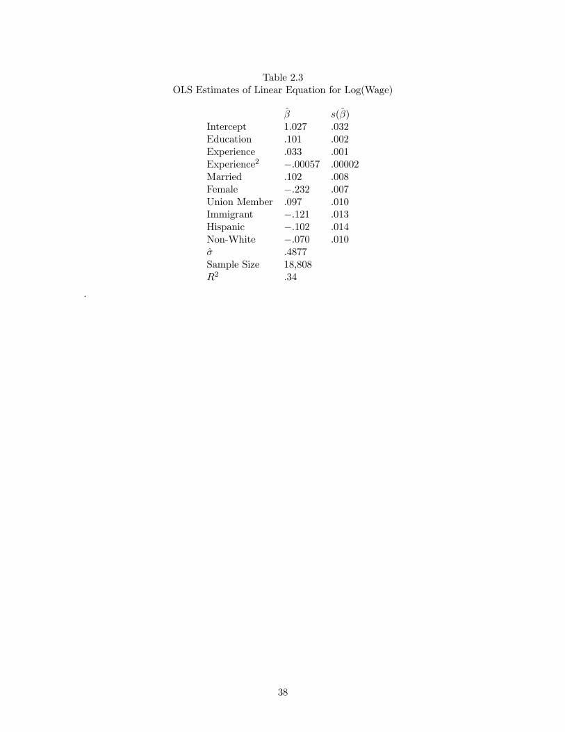
Table 2.3
OLS Estimates of Linear Equation for Log(Wage)
β s(β)Intercept 1.027 .032
Education .101 .002
Experience .033 .001
Experience2 −.00057 .00002
Married .102 .008
Female −.232 .007
Union Member .097 .010
Immigrant −.121 .013
Hispanic −.102 .014
Non-White −.070 .010
σ .4877
Sample Size 18,808
R2 .34
.
38
Chapter 3
Regression Estimation
This chapter explores estimation and inference in the regression model
yi = m(xi) + εi. (3.1)
E (εi | xi) = 0.
3.1 Linear Regression
An important special case of (3.1) is when the conditional mean function is linear in x. In this case
yi = x0iβ + εi (3.2)
E (ei | xi) = 0. (3.3)
Equation (3.2) is called the linear regression model, and is a special case of the projection
model. Indeed, E (εi | xi) = 0 implies uncorrelatedness E (xiεi) = 0, but not the converse. Forexample, suppose that for xi ∈ R that Ex3i = 0 and ei = x2i , Then Exie
2i = Ex3i = 0 yet
E (ei | xi) = x2i 6= 0.An important special case is homoskedastic linear regression model
yi = x0iβ + εi
E (εi | xi) = 0
E¡ε2i | xi
¢= σ2.
In this setting, by the law of iterated expectations
E¡xix
0iε2i
¢= E
¡xix
0iE¡ε2i | xi
¢¢= Qσ2
which is (2.21). Thus the homoskedastic linear regression model is also a special case of the
homoskedastic projection error model.
3.2 Bias and Variance of OLS estimator
The conditional mean assumption allows us to calculate the small sample conditional mean and
variance of the OLS estimator.
39
To examine the bias of β, using (2.13), the conditioning theorem, and the independence of the
observations
E³β − β | X
´= E
⎡⎣Ã nXi=1
xix0i
!−1 nXi=1
xiεi | X⎤⎦
=
ÃnXi=1
xix0i
!−1 nXi=1
xiE (εi | X)
=
ÃnXi=1
xix0i
!−1 nXi=1
xiE (εi | xi)
= 0
Thus the OLS estimator β is unbiased for β.
To examine its covariance matrix, for a random vector Y we define
V ar(Y ) = E (Y −EY ) (Y −EY )0
= EY Y 0 − (EY ) (EY )0 .Then by independence of the observations
V ar
ÃnXi=1
xiεi | X!=
nXi=1
V ar (xiεi | X) =nXi=1
xix0iσ2i
and we find
V ar³β | X
´=
ÃnXi=1
xix0i
!−1Ã nXi=1
xix0iσ2i
!ÃnXi=1
xix0i
!−1.
In the special case of the linear homoskedastic regression model, σ2i = σ2 and the covariance
matrix simplifies to
V ar³β | X
´=
ÃnXi=1
xix0i
!−1σ2.
Recall the method of moments estimator σ2 for σ2. We now calculate its finite sample bias
in the context of the homoskedastic linear regression model. Using (2.16) and linear algebra
manipulations
E¡nσ2 | X¢ = E
¡ε0Mε | X¢
= E¡tr¡ε0Mε
¢ | X¢= E
¡tr¡Mεε0
¢ | X¢= tr
£E¡Mεε0 | X¢¤
= tr£ME
¡εε0 | X¢¤
= tr£Mσ2
¤= σ2(n− k − 1),
the final equality by (B.4). We have found that under these assumptions
Eσ2 =(n− k − 1)
nσ2
40
so σ2 is biased towards zero. Since the bias is proportional to σ2, it is common to define the
bias-corrected estimator
s2 =1
n− k
nXi=1
e2i
so that Es2 = σ2 is unbiased. It is important to remember, however, that this estimator is only
unbiased in the special case of the homoskedastic linear regression model. It is not unbiased in the
absence of homoskedasticity, or in the projection model.
3.3 Forecast Intervals
In the linear regression model the conditional mean of yi given xi = x is
m(x) = E (yi | xi = x) = x0β.
In some cases, we want to estimate m(x) at a particular point x. Notice that this is a (linear)function of β. Letting h(β) = x0β and θ = h(β), we see that m(x) = θ = x0β and Hβ = x, so
s(θ) =pn−1x0V x. Thus an asymptotic 95% confidence interval for m(x) ish
x0β ± 2pn−1x0V x
i.
It is interesting to observe that if this is viewed as a function of x, the width of the confidence set
is dependent on x.
For a given value of xi = x, we may want to forecast (guess) yi out-of-sample. A reasonable
rule is the conditional mean m(x) as it is the mean-square-minimizing forecast. A point forecastis the estimated conditional mean m(x) = x0β. We would also like a measure of uncertainty forthe forecast.
The forecast error is ei = yi − m(x) = εi − x0³β − β
´. As the out-of-sample error εi is
independent of the in-sample estimate β, this has variance
Ee2i = E¡ε2i | xi = x
¢+ x0E
³β − β
´³β − β
´0x
= σ2(x) + n−1x0V x.
Assuming E¡ε2i | xi
¢= σ2, the natural estimate of this variance is σ2 + n−1x0V x, so a standard
error for the forecast ispσ2 + n−1x0V x. Notice that this is different from the standard error for
the conditional mean.
It would appear natural to conclude that an asymptotic 95% forecast interval for yi is∙x0β ± 2
qσ2 + n−1x0V x
¸,
but this turns out to be incorrect. In general, the validity of an asymptotic confidence interval is
based on the asymptotic normality of the studentized ratio. In the present case, this would require
the asymptotic normality of the ratio
εi − x0³β − β
´pσ2 + n−1x0V x
.
41
But no such asymptotic approximation can be made. The only special exception is the case where
εi has the exact distribution N(0, σ2), which is generally invalid.To get an accurate forecast interval, we need to estimate the conditional distribution of εi given
xi = x, which is a much more difficult task. Given the difficulty, most applied forecasters focus on
the simple and unjustified intervalhx0β ± 2
pσ2 + n−1x0V x
i.
3.4 Normal Regression Model
The normal regression model adds the additional assumption that the error εi is independent of xiand has distribution N(0, σ2). This is a parametric model, where likelihood methods can be usedfor estimation, testing, and distribution theory.
The log-likelihood function for the normal regression model is
Ln(β, σ2) =
nXi=1
log
Ã1
(2πσ2)1/2exp
µ− 1
2σ2¡yi − x0iβ
¢2¶!
= −n2log¡2πσ2
¢− 1
2σ2
nXi=1
¡yi − x0iβ
¢2The MLE (β, σ2) maximize Ln(β, σ
2). Since Ln(β, σ2) is a function of β only through the sum
of squared errors, maximizing the likelihood is identical to minimizing the sum of squared errors.
Hence the MLE for β equals the OLS estimator β = (X 0X)−1(X 0Y ).Plugging this estimator into the log-likelihood we obtain
Ln(β, σ2) = −n
2log¡2πσ2
¢− 1
2σ2
nXi=1
e2i
Maximization with respect to σ2 yields the first-order condition
∂
∂σ2Ln(β, σ
2) = − n
2σ2+
1
2¡σ2¢2 e0e = 0.
Solving for σ2 yields
σ2 =1
ne0e.
which is identical to the method of moments estimator. Thus the estimators are not affected by
this assumption. Due to this equality, the OLS estimator β is frequently referred to as the Gaussian
MLE.
Under the normality assumption, we see that the error vector ε is independent of X and
has distribution N¡0, Inσ
2¢. Since linear functions of normals are also normal, this implies that
conditional on Xµβ − β
e
¶=
µ(X 0X)−1X 0
M
¶ε ∼ N
µ0,
µσ2 (X 0X)−1 0
0 σ2M
¶¶where M = I − X (X 0X)−1X 0. Since uncorrelated normal variables are independent, it followsthat β is independent of any function of the OLS residuals, including the estimated error variance
s2.
42
The spectral decomposition of M yields
M = H
∙In−k−1 00 0
¸H 0
(see equation (B.5)) where H 0H = In. Let u = σ−1H 0ε ∼ N (0,H 0H) ∼ N (0, In) . Then
(n− k − 1) s2σ2
=1
σ2e0e
=1
σ2ε0Mε
=1
σ2ε0H
∙In−k−1 00 0
¸H 0ε
= u0∙In−k−1 00 0
¸u
∼ χ2n−k−1,
a chi-square distribution with n − k degrees of freedom. Furthermore, if standard errors are
calculated using the homoskedastic formula (2.23)
βj − βj
s(βj)=
βj − βj
s
rh(X 0X)−1
ijj
∼N
µ0, σ2
h(X 0X)−1
ijj
¶q
σ2
n−k−1χ2n−k−1
rh(X 0X)−1
ijj
=N (0, 1)qχ2n−k−1n−k−1
∼ tn−k−1
a t distribution with n− k − 1 degrees of freedom.We summarize these findings
Theorem 3.4.1 If εi is independent of xi and distributed N(0, σ2), and standard errors are cal-culated using the homoskedastic formula (2.23) then
• β ∼ N³0, σ2 (X 0X)−1
´• (n−k)s2
σ2∼ χ2n−k−1,
• βj−βjs(βj)
∼ tn−k−1
In Theorem 2.7.1 and Theorem 2.13.1 we showed that in large samples, β and t are approxi-
mately normally distributed. In contrast, Theorem 3.4.1 shows that under the strong assumption
of normality, β has an exact normal distribution and t has an exact t distribution. As inference
(confidence intervals) are based on the t-ratio, the notable distinction is between the N(0, 1) andtn−k−1 distributions. The critical values are quite close if n− k− 1 ≥ 30, so as a practical matterit does not matter which distribution is used. (Unless the sample size is unreasonably small.)
Now let us partition β = (β1, β2) and consider tests of the linear restriction
H0 : β2 = 0
H1 : β2 6= 0
43
In the context of parametric models, a good testing procedure is based on the likelihood ra-
tio statistic, which is twice the difference in the log-likelihood function evaluated under the null
and alternative hypotheses. The estimator under the alternative is the unrestricted estimator
(β1, β2, σ2) discussed above. The log-likelihood at these estimates is
Ln(β1, β2, σ2) = −n
2log¡2πσ2
¢− 1
2σ2e0e
= −n2log¡σ2¢− n
2log (2π)− n
2.
The MLE of the model under the null hypothesis is (β1, 0, σ2) where β1 is the OLS estimate from
a regression of yi on x1i only, with residual variance σ2. The log-likelihood of this model is
Ln(β1, 0, σ2) = −n
2log¡σ2¢− n
2log (2π)− n
2.
The LR statistic for H0 is
LR = 2³Ln(β1, β2, σ
2)− Ln(β1, 0, σ2)´
= n¡log¡σ2¢− log ¡σ2¢¢
= n log
µσ2
σ2
¶.
By a first-order Taylor series approximation
LR = n log
µ1 +
σ2
σ2− 1¶' n
µσ2
σ2− 1¶=Wn.
the F statistic.
3.5 GLS and the Gauss-Markov Theorem
The linear regression model
yi = x0iβ + εi
E (εi | xi) = 0
imposes the condition of zero conditional mean. This is stronger than the orthogonality condition
E (xiεi) = 0. This stronger condition can be exploited to improve estimation efficiency. Recall thedefinition of the conditional variance σ2i = E
¡ε2i | xi
¢.
The Generalized Least Squares (GLS) estimator of β is
β =¡X 0D−1X
¢−1 ¡X 0D−1Y
¢(3.4)
where
D = diagσ21, ..., σ2n =
⎛⎜⎜⎜⎝σ21 0 · · · 00 σ22 · · · 0...
.... . .
...
0 0 · · · σ2n
⎞⎟⎟⎟⎠ .
The GLS estimator is sometimes called the Aitken estimator.
44
Since Y = Xβ + ε, then
β = β +¡X 0D−1X
¢−1 ¡X 0D−1ε
¢.
Since D is a function of X, E³β | X
´= β and
V ar(β | X) =¡X 0D−1X
¢−1X 0D−1DD−1X
¡X 0D−1X
¢−1=
¡X 0D−1X
¢−1.
The class of unbiased linear estimators take the form
βL = A(X)0Y, A(X)0X = Ik
where A(X), n × k, is a function only of X. This is called linear because it is a linear function
of Y, even though it is nonlinear in X. OLS is the case A(X) = X(X 0X)−1 and GLS is the caseA(X) = D−1X
¡X 0D−1X
¢−1. Observe that
E³βL | X
´= A(X)0Xβ = β
so βL is unbiased. Thus βL = β +A(X)0ε, and its variance is
V ar(βL | X) = A(X)0DA(X).
The “best” estimator within this class is the one with the smallest variance.
Theorem 3.5.1 Gauss-Markov. The best (minimum-variance) unbiased linear estimator is
GLS.
Proof. Let A∗ = D−1X¡X 0D−1X
¢−1and A be any other n × k function of X such that
A0X = Ik. We need to show that A0DA ≥ A∗0DA∗.
Let C = A−A∗. Note that
C0X = A0X −A∗0X= Ik − Ik = 0
and
C0DA∗ = C0DD−1X¡X 0D−1X
¢−1= C0X
¡X 0D−1X
¢−1= 0.
Then
A0DA = (C +A∗)0D (C +A∗)= C 0DC +C 0DA∗ +A∗0DC +A∗0DA∗
= C 0DC +A∗0DA∗ ≥ A∗DA∗0.
¥
The Gauss-Markov theorem tells us that the OLS estimator is inefficient in linear regression
models, and that within the class of linear estimators, GLS is efficient. However, the restriction
45
to linear estimators is unsatisfactory, as the theorem leaves open the possibility that a non-linear
estimator could have lower mean squared error than the GLS estimator.
Chamberlain (1987) established a more powerful and general result. He showed that in the
regression model, no regular consistent estimator can have a lower asymptotic variance than the
GLS estimator. This establishes that the GLS estimator is asymptotically efficient. The proof of
his theorem is quite deep and we cannot cover it here.
In Section 2.5 we claimed that OLS is asymptotically efficient in the class of models with
E (xiεi) = 0. Now we have shown that OLS is inefficient if E (εi | xi) = 0. The gain of efficiency(through use of GLS) comes through the exploitation of the stronger conditional mean assumption,
which has the cost of reduced robustness. If E (ei | xi) 6= 0 then the GLS estimator will beinconsistent for the projection coefficient β, but OLS will be consistent.
3.6 Least Absolute Deviations
We stated that a conventional goal in econometrics is estimation of impact of variation in xi on
the central tendency of yi.We have discussed projections and conditional means, but these are not
the only measures of central tendency. An alternative good measure is the conditional median.
To recall the definition and properties of the median, let Y be a continuous random variable.
The median θ0 = Med(Y ) is the value such that P (Y ≤ θ0) = P (Y ≥ θ0) = .5. Two useful factsabout the median are that
θ0 = minθ
E |Y − θ|and
E sgn (Y − θ0) = 0
where
sgn (u) =
½1 if u ≥ 0−1 if u < 0
is the sign function.
These three definitions motivate three estimators of θ. The first suggests taking the 50th quan-
tile. The second suggests finding the solution to the moment equation 1n
Pni=1 sgn (yi − θ) , and
the first suggests minimizing 1n
Pni=1 |yi − θ| . These distinctions are illusory, however, as these
estimators are indeed identical.
Now let’s consider the conditional median of Y given a random variable X. Let m(x) =Med (Y | X = x) denote the conditional median of Y given X = x, and let Med (Y | X) = m(X)be this function evaluated at the random variable X. The linear median regression model takes
the form
yi = x0iβ + ui
Med (ui | xi) = 0
In this model, the linear function Med (yi | xi = x) = x0β is the conditional median function, andthe substantive assumption is that the median function is linear in x.
Conditional analogs of the facts about the median are
• P (yi ≤ x0β0 | xi = x) = P (yi > x0β | xi = x) = .5
• E (sgn (ui) | xi) = 0
46
• E (xi sgn (ui)) = 0
• β0 = minβ E |yi − x0iβ|
These facts motivate the following estimator. Let
Ln(β) =1
n
nXi=1
¯yi − x0iβ
¯be the average of absolute deviations. The least absolute deviations (LAD) estimator of β
minimizes this function
β = argminβ
Ln(β)
Equivalently, it is a solution to the moment condition
1
n
nXi=1
xi sgn³yi − x0iβ
´= 0. (3.5)
Let f (u | x) denote the conditional density of ui given xi = x. The LAD estimator has the
asymptotic distribution
Theorem 3.6.1√n³β − β0
´→d N(0, V ),
V =1
4
¡E¡xix
0if (0 | xi)
¢¢−1 ¡Exix
0i
¢ ¡E¡xix
0if (0 | xi)
¢¢−1The variance of the asymptotic distribution inversely depends on f (0 | x) , the conditional
density of the error at its median. When f (0 | x) is large, then there are many innovations nearto the median, and this improves estimation of the median. In the special case where the error is
independent of xi, then f (0 | x) = f (0) and the asymptotic variance simplifies
V =(Exix
0i)−1
4f (0)2(3.6)
This simplification is similar to the simplification of the asymptotic covariance of the OLS estimator
under homoskedasticity.
Computation of standard error for LAD estimates typically is based on equation (3.6). The
main difficulty is the estimation of f(0), the height of the error density at its median. This canbe done with kernel estimation techniques. See Chapter 12. While a complete proof of Theorem
3.6.1 is advanced, we provide a sketch here for completeness.
Proof : Since sgn (a) = 1 − 2 · 1 (a ≤ 0) , (3.5) is equivalent to gn(β) = 0, where gn(β) =n−1
Pni=1 gi(β) and gi(β) = xi (1− 2 · 1 (yi ≤ x0iβ)) . Let g(β) = Egi(β). We need three preliminary
result. First, by the central limit theorem (Theorm D.4.1)
√n (gn(β0)− g(β0)) = −n−1/2
nXi=1
gi(β0)→d N(0, Exix0i)
47
since Egi(β0)gi(β0)0 = Exix
0i. Second using the law of iterated expectations and the chain rule of
differentiation,
∂
∂β0g(β) =
∂
∂β0Exi
¡1− 2 · 1 ¡yi ≤ x0iβ
¢¢= −2 ∂
∂β0E£xiE
¡1¡ui ≤ x0iβ − x0iβ0
¢ | xi¢¤= −2 ∂
∂β0E
"xi
Z x0iβ−x0iβ0
−∞f (u | xi) du
#= −2E £xix0if ¡x0iβ − x0iβ0 | xi
¢¤so
∂
∂β0g(β0) = −2E
£xix
0if (0 | xi)
¤.
Third, by a Taylor series expansion and the fact g(β0) = 0
g(β) ' ∂
∂β0g(β0)
³β − β0
´.
Together
√n³β − β0
´'
µ∂
∂β0g(β0)
¶−1√ng(β)
=¡−2E £xix0if (0 | xi)¤¢−1√n³g(β)− gn(β)
´' 1
2
¡E£xix
0if (0 | xi)
¤¢−1√n (gn(β0)− g(β0))
→ d1
2
¡E£xix
0if (0 | xi)
¤¢−1N(0, Exix
0i)
= N(0, V ).
The third line follows from an asymptotic empirical process argument.
3.7 NonLinear Least Squares
In some cases we might use a parametric regression function m(x, θ) = E (yi | xi = x) which isa non-linear function of the parameters θ. We describe this setting as non-linear regression.
Examples of nonlinear regression functions include
m(x, θ) = θ1 + θ2x
1 + θ3x
m(x, θ) = θ1 + θ2xθ3
m(x, θ) = θ1 + θ2 exp(θ3x)
m(x, θ) = G(x0θ), G known
m(x, θ) = θ1 + θ2x1 + (θ3 + θ4x1)Φ
µx2 − θ5
θ6
¶m(x, θ) = θ1 + θ2x+ θ4 (x− θ3) 1 (x > θ3)
m(x, θ) = (θ1 + θ2x1) 1 (x2 < θ3) + (θ4 + θ5x1) 1 (x2 > θ3)
48
In the first five examples, m(x, θ) is (generically) differentiable in the parameters θ. In the finaltwo examples, m is not differentiable with respect to θ3, which alters some of the analysis. When
it exists, let
mθ(x, θ) =∂
∂θm(x, θ).
Nonlinear regression is frequently adopted because the functional form m(x, θ) is suggestedby an economic model. In other cases, it is adopted as a flexible approximation to an unknown
regression function.
The least squares estimator θ minimizes the sum-of-squared-errors
Sn(θ) =nXi=1
(yi −m(xi, θ))2 .
When the regression function is nonlinear, we call this the nonlinear least squares (NLLS)
estimator. The NLLS residuals are ei = yi −m(xi, θ).One motivation for the choice of NLLS as the estimation method is that the parameter θ is
the solution to the population problem minθ E (yi −m(xi, θ))2
Since sum-of-squared-errors function Sn(θ) is not quadratic, θ must be found by numericalmethods. See Appendix E. When m(x, θ) is differentiable, then the FOC for minimization are
0 =nXi=1
mθ(xi, θ)ei. (3.7)
Theorem 3.7.1 If the model is identified and m(x, θ) is differentiable with respect to θ,
√n³θ − θ0
´→d N(0, V )
V =¡E¡mθim
0θi
¢¢−1 ¡E¡mθim
0θiε
2i
¢¢ ¡E¡mθim
0θi
¢¢−1where mθi = mθ(xi, θ0).
Sketch of Proof. First, it must be shown that θ →p θ0. This can be done using arguments
for optimization estimators, but we won’t cover that argument here. Since θ →p θ0, θ is close to
θ0 for n large, so the minimization of Sn(θ) only needs to be examined for θ close to θ0. Let
y0i = εi +m0θiθ0.
For θ close to the true value θ0, by a first-order Taylor series approximation,
m(xi, θ) ' m(xi, θ0) +m0θi (θ − θ0) .
Thus
yi −m(xi, θ) ' (εi +m(xi, θ0))−¡m(xi, θ0) +m0
θi (θ − θ0)¢
= εi −m0θi (θ − θ0)
= y0i −m0θiθ.
Hence the sum of squared errors function is
Sn(θ) =nXi=1
(yi −m(xi, θ))2 '
nXi=1
¡y0i −m0
θiθ¢2
49
and the right-hand-side is the SSE function for a linear regression of y0i on mθi. Thus the NLLS
estimator θ has the same asymptotic distribution as the (infeasible) OLS regression of y0i on mθi,
which is that stated in the theorem. ¥
Based on Theorem 3.7.1, an estimate of the asymptotic variance V is
V =
Ã1
n
nXi=1
m0θi
!−1Ã1
n
nXi=1
mθim0θie
2i
!Ã1
n
nXi=1
mθim0θi
!−1where mθi = mθ(xi, θ) and ei = yi −m(xi, θ).
Identification is often tricky in nonlinear regression models. Suppose that
m(xi, θ) = β01zi + β02xi(γ).
The model is linear when β2 = 0, and this is often a useful hypothesis (sub-model) to consider.Thus we want to test
H0 : β2 = 0.
However, under H0, the model is
yi = β01zi + εi
and both β2 and γ have dropped out. This means that under H0, γ is not identified. This renders
the distribution theory presented in the previous section invalid. Thus when the truth is that
β2 = 0, the parameter estimates are not asymptotically normally distributed. Furthermore, testsof H0 do not have asymptotic normal or chi-square distributions.
The asymptotic theory of such tests have been worked out by Andrews and Ploberger (1994)
and B. Hansen (1996). In particular, Hansen shows how to use simulation (similar to the bootstrap)
to construct the asymptotic critical values (or p-values) in a given application.
3.8 Testing for Omitted NonLinearity
If the goal is to estimate the conditional expectation E (yi | xi) , it is useful to have a general testof the adequacy of the specification.
One simple test for neglected nonlinearity is to add nonlinear functions of the regressors to
the regression, and test their significance using a Wald test. Thus, if the model yi = x0iβ + ei has
been fit by OLS, let zi = h(xi) denote functions of xi which are not linear functions of xi (perhapssquares of non-binary regressors) and then fit yi = x0iβ+z0iγ+ ei by OLS, and form a Wald statisticfor γ = 0.
Another popular approach is the RESET test proposed by Ramsey (1969). The null model is
yi = x0iβ + εi
which is estimated by OLS, yielding predicted values yi = x0iβ. Now let
zi =
⎛⎜⎝ y2i...
ymi
⎞⎟⎠be an (m− 1)-vector of powers of yi. Then run the auxiliary regression
yi = x0iβ + z0iγ + ei (3.8)
50
by OLS, and form the Wald statistic Wn for γ = 0. It is easy (although somewhat tedious) toshow that under the null hypothesis, Wn →d χ
2m−1. Thus the null is rejected at the α% level if Wn
exceeds the upper α% tail critical value of the χ2m−1 distribution.To implement the test, m must be selected in advance. Typically, small values such as m = 2,
3, or 4 seem to work best.
The RESET test appears to work well as a test of functional form against a wide range of
smooth alternatives. It is particularly powerful at detecting single-index models of the form
yi = G(x0iβ) + εi
where G(·) is a smooth “link” function. To see why this is the case, note that (3.8) may be writtenas
yi = x0iβ +³x0iβ´2
γ1 +³x0iβ´3
γ2 + · · ·³x0iβ´m
γm−1 + ei
which has essentially approximated G(·) by a m’th order polynomial
3.9 Model Selection
In Chapter 2 we discussed the costs and benefits of inclusion/exclusion of variables. How does a
researcher go about selecting an econometric specification, when economic theory does not provide
complete guidance? This is the question of model selection. It is important that the model selection
question be well-posed. For example, the question: “What is the right model for y?” is not well
posed, because it does not make clear the conditioning set. In contrast, the question, “Which
subset of (x1, ..., xK) enters the regression function E(yi | x1i = x1, ..., xKi = xK)?” is well posed.In many cases the problem of model selection can be reduced to the comparison of two nested
models, as the larger problem can be written as a sequence of such comparisons. We thus consider
the question of the inclusion of X2 in the linear regression
Y = X1β1 +X2β2 + ε,
where X1 is n× k1 and X2 is n× k2. This is equivalent to the comparison of the two models
M1 : Y = X1β1 + ε, E (ε | X1,X2) = 0
M2 : Y = X1β1 +X2β2 + ε, E (ε | X1,X2) = 0.
Note thatM1 ⊂M2. To be concrete, we say thatM2 is true if β2 6= 0.To fix notation, models 1 and 2 are estimated by OLS, with residual vectors e1 and e2, estimated
variances σ21 and σ22, etc., respectively. To simplify some of the statistical discussion, we will on
occasion use the homoskedasticity assumption E¡ε2i | x1i, x2i
¢= σ2.
A model selection procedure is a data-dependent rule which selects one of the true models. We
can write this as cM. There are many possible desirable properties for a model selection procedure.
One useful property is consistency, that it selects the true model with probability one if the sample
is sufficiently large. A model selection procedure is consistent if
P³cM =M1 | M1
´→ 1
P³cM =M2 | M2
´→ 1
We now discuss a number of possible model selection methods.
51
Selection Based on Fit
Natural measures of fit of a regression are the residual sum of squares e0e, R2 = 1− (e0e) /σ2y orGaussian log-likelihood l = −(n/2) log σ2. It might therefore be thought attractive to base a modelselection procedure on one of these measures of fit. The problem is that each of these measures
are necessarily monotonic between nested models, namely e01e1 ≥ e02e2, R21 ≤ R22, and l1 ≤ l2, so
modelM2 would always be selected, regardless of the actual data and probability structure. This
is clearly an inappropriate decision rule!
Selection based on Testing
A common approach to model selection is to base the decision on a statistical test such as
the Wald Wn. The model selection rule is as follows. For some critical level α, let cα satisfy
P¡χ2k2 > cα
¢. Then selectM1 if Wn ≤ cα, else selectM2.
The major problem with this approach is that the critical level α is indeterminate. The rea-
soning which helps guide the choice of α in hypothesis testing (controlling Type I error) is not
relevant for model selection. That is, if α is set to be a small number, then P³cM =M1 | M1
´≈
1 − α but P³cM =M2 | M2
´could vary dramatically, depending on the sample size, etc. An-
other problem is that if α is held fixed, then this model selection procedure is inconsistent, as
P³cM =M1 | M1
´→ 1− α < 1.
Adjusted R-squared
While R2 is necessarily increasing in the model size, this is not true for Theils adjusted R2.
Because of this distinction, it was at one time popular to pick between models based on R2. This
rule is to select M1 if R21 > R
22, else select M2. Since R
2is a monotonically decreasing function
of s2, this rule is the same as selecting the model with the smaller s2, or equivalently, the smaller
log(s2). It is helpful to observe that
log(s2) = log
µσ2
n
n− k
¶= log
¡σ2¢+ log
µ1 +
k
n− k
¶' log
¡σ2¢+
k
n− k
' log¡σ2¢+
k
n,
(the first approximation is log(1 + x) ' x for small x). Thus selecting based on R2is essentially
the same as selecting based on log¡σ2¢+ k
n, which is a particular choice of penalized likelihood
criteria. It turns out that model selection based on any criterion of the form
log¡σ2¢+ c
k
n, c > 0, (3.9)
is inconsistent, as the rule tends to overfit. Indeed, since underM1,
LRn = n¡log σ21 − log σ22
¢ 'Wn →d χ2k2, (3.10)
52
P³cM =M1 | M1
´= P
³R21 > R
22 | M1
´' P
¡n log(s21) < n log(s22) | M1
¢' P
¡n log
¡σ21¢+ ck1 < n log
¡σ22¢+ c (k1 + k2) | M1
¢= P (LRn < ck2 | M1)
→ P¡χ2k2 < ck2
¢< 1.
Akaike Information Criterion
Akaike proposed an information criterion which takes the form (3.9) with c = 2 :
AIC = log¡σ2¢+ 2
k
n. (3.11)
This imposes a larger penalty on overparameterization than does R2. Akaike’s motivation for
this criterion is that a good measure of the fit of a model density f(Y | X,M) to the truedensity f(Y | X) is the Kullback distance K(M) = E (log f(Y | X)− log f(Y | X,M)) . The log-likelihood function provides a decent estimate of this distance, but it is biased, and a better,
less-biased estimate can be obtained by introducing the penalty 2k. The actual derivation is notvery enlightening, and the motivation for the argument is not fully satisfactory, so we omit the
details. Despite these concerns, the AIC is a popular method of model selection. The rule is to
selectM1 if AIC1 < AIC2, else selectM2.
Since the AIC criterion (3.11) takes the form (3.9), it is an inconsistent model selection criterion,
and tends to overfit.
Schwarz Criterion
While many modifications of the AIC have been proposed, the most popular appears to be one
proposed by Schwarz, based on Bayesian arguments. His criterion, known as the BIC, is
BIC = log¡σ2¢+ log(n)
k
n. (3.12)
Since log(n) > 2 (if n > 8), the BIC places a larger penalty than the AIC on the number of
estimated parameters and is more parsimonious.
In contrast to the other methods studied above, BIC model selection is consistent. Indeed,
since (3.10) holds underM1,LRn
log(n)→p 0,
so
P³cM =M1 | M1
´= P (BIC1 < BIC2 | M1)
= P (LRn < log(n)k2 | M1)
= P
µLRn
log(n)< k2 | M1
¶→ P (0 < k2) = 1.
Also underM2, one can show thatLRn
log(n)→p ∞,
53
thus
P³cM =M2 | M2
´= P
µLRn
log(n)> k2 | M2
¶→ 1.
Selection Among Multiple Regressors
We have discussed model selection between two models. The methods extend readily to the
issue of selection among multiple regressors. The general problem is the model
yi = β1x1i + β2x1i + · · ·+ βKxKi + εi, E (εi | xi) = 0
and the question is which subset of the coefficients are non-zero (equivalently, which regressors
enter the regression).
There are two leading cases: ordered regressors and unordered.
In the ordered case, the models are
M1 : β1 6= 0, β2 = β3 = · · · = βK = 0
M2 : β1 6= 0, β2 6= 0, β3 = · · · = βK = 0...
MK : β1 6= 0, β2 6= 0, . . . , βK 6= 0.
which are nested. The AIC selection criteria estimates the K models by OLS, stores the residual
variance σ2 for each model, and then selects the model with the lowest AIC (3.11). Similarly for
the BIC, selecting based on (3.12).
In the unordered case, a model consists of any possible subset of the regressors x1i, ..., xKi,and the AIC or BIC in principle can be implemented by estimating all possible subset models.
However, there are 2K such models, which can be a very large number. For example, 210 = 1024,and 220 = 1, 048, 576. In the latter case, a full-blown implementation of the BIC selection criterionwould seem computationally prohibitive.
54
Chapter 4
The Bootstrap
4.1 Definition of the Bootstrap
Let F denote a distribution function for the population of observations (yi, xi) . Let θ be someparameter of interest, which is a function of the distribution F. Let Tn = Tn(y1, x1,..., yn, xn, θ) be
a statistic of interest, for example an estimator θ or a t-statistic³θ − θ
´/s(θ).
The exact CDF of Tn when the data are sampled from the distribution F is
Gn(x,F ) = P (Tn ≤ x | F )Given the structure of the problem, Gn is a function only of F. In general, Gn(x,F ) depends onF, meaning that G changes as F changes.
Ideally, inference on θ would be based on Gn(x,F ). This is generally impossible since F is
unknown.
Asymptotic inference is based on approximating Gn(x, F ) with G(x, F ) = limn→∞Gn(x,F ).When G(x,F ) = G(x) does not depend on F, we say that Tn is asymptotically pivotal and use thedistribution function G(x) for inferential purposes.
In a seminal contribution, Efron (1979) proposed the bootstrap, which makes a different ap-
proximation. The unknown F is replaced by an estimate Fn (one choice is discussed in the next
section), and plugged into Gn(x, F ) to obtain
G∗n(x) = Gn(x,Fn). (4.1)
The bootstrap substitutes Fn for F in the formula Gn(x,F ). As such, it not only pretendsthat the distribution of (yi, xi) is Fn rather than F, but it also pretends that the true value of theparameter1 is the sample estimate θ, rather than the true value of θ.
Let T ∗n = Tn(y∗1, x
∗1, ..., y
∗n, x
∗n, θ) be a random variable with distribution G∗n. That is,
P (T ∗n ≤ x) = G∗n(x).
We call (y∗i , x∗i ), T ∗n , and G∗n the bootstrap data, statistic, and distribution. T ∗n is the correctanalog of Tn when the true CDF is Fn, as the data (y∗i , x∗i ) are sampled from the CDF Fn and the
parameter θ is the true value under Fn. The bootstrap distribution is a random distribution, as it
depends on the sample through the estimator Fn. Bootstrap inference is based on G∗n(x).In the next sections we describe computation of the bootstrap distribution.
1More precisely, the bootstrap pretends that the true value of θ is the value consistent with Fn, the estimate ofF used to construct the bootstrap. In most cases, and the ones we consider, this value of θ is the sample estimate θ.
55
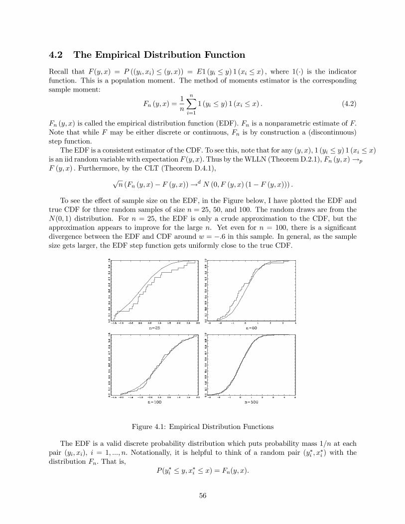
4.2 The Empirical Distribution Function
Recall that F (y, x) = P ((yi, xi) ≤ (y, x)) = E1 (yi ≤ y) 1 (xi ≤ x) , where 1(·) is the indicatorfunction. This is a population moment. The method of moments estimator is the corresponding
sample moment:
Fn (y, x) =1
n
nXi=1
1 (yi ≤ y) 1 (xi ≤ x) . (4.2)
Fn (y, x) is called the empirical distribution function (EDF). Fn is a nonparametric estimate of F.Note that while F may be either discrete or continuous, Fn is by construction a (discontinuous)
step function.
The EDF is a consistent estimator of the CDF. To see this, note that for any (y, x), 1 (yi ≤ y) 1 (xi ≤ x)is an iid random variable with expectation F (y, x).Thus by theWLLN (TheoremD.2.1), Fn (y, x)→p
F (y, x) . Furthermore, by the CLT (Theorem D.4.1),
√n (Fn (y, x)− F (y, x))→d N (0, F (y, x) (1− F (y, x))) .
To see the effect of sample size on the EDF, in the Figure below, I have plotted the EDF and
true CDF for three random samples of size n = 25, 50, and 100. The random draws are from the
N(0, 1) distribution. For n = 25, the EDF is only a crude approximation to the CDF, but theapproximation appears to improve for the large n. Yet even for n = 100, there is a significantdivergence between the EDF and CDF around w = −.6 in this sample. In general, as the samplesize gets larger, the EDF step function gets uniformly close to the true CDF.
Figure 4.1: Empirical Distribution Functions
The EDF is a valid discrete probability distribution which puts probability mass 1/n at eachpair (yi, xi), i = 1, ..., n. Notationally, it is helpful to think of a random pair (y∗i , x
∗i ) with the
distribution Fn. That is,
P (y∗i ≤ y, x∗i ≤ x) = Fn(y, x).
56
We can easily calculate the moments of (y∗i , x∗i ) :
Eh (y∗i , x∗i )) =
Zh(y, x)dFn(y, x)
=nXi=1
h (yi, xi)P (y∗i = yi, x
∗i = xi)
=1
n
nXi=1
h (yi, xi) ,
the empirical sample average.
4.3 Nonparametric Bootstrap
The nonparametric bootstrap is obtained when the bootstrap distribution (4.1) is defined using
the EDF (4.2) as the estimate Fn of F. Since Fn is a consistent estimator for F, G∗n(x) = Gn(x,Fn)
is consistent for Gn(x,F ).Since the EDF Fn is a multinomial (with n support points), in principle the distribution G∗n
could be calculated by direct methods. Since there are 2n possible samples (y∗1, x∗1) , ..., (y∗n, x∗n),however, such a calculation is computationally infeasible unless n is very small. The popular
alternative is to use Monte Carlo simulation to approximate the distribution. The algorithm is
identical to our discussion of Monte Carlo simulation, with the following points of clarification:
• The sample size n used for the simulation is the same as the sample size.• The random vectors (y∗i , x
∗i ) are drawn randomly from the empirical distribution. This is
equivalent to sampling a pair (yi, xi) randomly from the sample.
• T ∗n = Tn(y∗1, x
∗i , ..., y
∗n, x
∗n, θ) is evaluated at the sample estimate θ.
If an estimate of F other than the EDF is used, the second step above is replaced by random
sampling from that estimate. Notice, however, that sampling from the EDF is particularly easy.
Since Fn is a discrete probability distribution putting probability mass 1/n at each sample point,sampling from the EDF is equivalent to random sampling a pair (yi, xi) from the observed data
with replacement. In consequence, a bootstrap sample y∗1, x∗1, ..., y∗n, x∗n will necessarily havesome ties and multiple values, which is generally not a problem.
A theory for the determination of the number of bootstrap replications B has been developed
by Andrews and Buchinsky (2000).
4.4 Bootstrap Estimation of Bias and Variance
The bias of θ is
τn = E(θ − θ0).
Let Tn(θ) = θ − θ. Then
τn = E(Tn(θ0)).
The bootstrap counterparts are θ∗= θ(y∗1, x∗1..., y∗n, x∗n) and T ∗n = θ
∗ − θn = θ∗ − θ. The bootstrap
estimate of τn is
τ∗n = E(T ∗n).
57
If this is calculated by the simulation described in the previous section, the estimate of τ∗n is
τ∗n =1
B
BXb=1
T ∗nb
=1
B
BXb=1
θ∗b − θ
= θ∗ − θ.
If θ is biased, it might be desirable to construct a biased-corrected estimator (one with reduced
bias). Ideally, this would be
θ = θ − τn,
but τn is unknown. The (estimated) bootstrap biased-corrected estimator is
θ∗= θ − τ∗n= θ − (θ∗ − θ)
= 2θ − θ∗.
Note, in particular, that the biased-corrected estimator is not θ∗. Intuitively, the bootstrap makes
the following experiment. Suppose that θ is the truth. Then what is the average value of θ
calculated from such samples? The answer is θ∗. If this is lower than θ, this suggests that the
estimator is downward-biased, so a biased-corrected estimator of θ should be larger than θ, and
the best guess is the difference between θ and θ∗. Similarly if θ
∗is higher than θ, then the estimator
is upward-biased and the biased-corrected estimator should be lower than θ.
Let Tn = θ. The variance of θ is
Vn = E(Tn −ETn)2.
Let T ∗n = θ∗. It has variance
V ∗n = E(T ∗n −ET ∗n)2.
The simulation estimate is
V ∗n =1
B
BXb=1
³θ∗b − θ
∗´2.
A bootstrap standard error for θ is the square root of the bootstrap estimate of variance,
s(β) =qV ∗n .
While this standard error may be calculated and reported, it is not clear if it is useful. The
primary use of asymptotic standard errors is to construct asymptotic confidence intervals, which
are based on the asymptotic normal approximation to the t-ratio. However, the use of the boot-
strap presumes that such asymptotic approximations might be poor, in which case the normal
approximation is suspected. It appears superior to calculate bootstrap confidence intervals, and
we turn to this next.
58
4.5 Percentile Intervals
For a distribution function Gn(x, F ), let qn(α,F ) denote its quantile function. This is the functionwhich solves
Gn(qn(α, F ), F ) = α.
[When Gn(x, F ) is discrete, qn(α,F ) may be non-unique, but we will ignore such complications.]Let qn(α) = qn(α, F0) denote the quantile function of the true sampling distribution, and q
∗n(α) =
qn(α,Fn) denote the quantile function of the bootstrap distribution. Note that this function willchange depending on the underlying statistic Tn whose distribution is Gn.
Let Tn = θ, an estimate of a parameter of interest. In (1−α)% of samples, θ lies in the region
[qn(α/2), qn(1− α/2)]. This motivates a confidence interval proposed by Efron:
C1 = [q∗n(α/2), q∗n(1− α/2)].
This is often called the percentile confidence interval.
Computationally, the quantile q∗n(x) is estimated by q∗n(x), the x’th sample quantile of the
simulated statistics T ∗n1, ..., T ∗nB, as discussed in the section on Monte Carlo simulation. The(1− α)% Efron percentile interval is then [q∗n(α/2), q∗n(1− α/2)].
The interval C1 is a popular bootstrap confidence interval often used in empirical practice.
This is because it is easy to compute, simple to motivate, was popularized by Efron early in the
history of the bootstrap, and also has the feature that it is translation invariant. That is, if we
define φ = f(θ) as the parameter of interest for a monotonic function f, then percentile method
applied to this problem will produce the confidence interval [f(q∗n(α/2)), f(q∗n(1−α/2))], whichis a naturally good property.
However, as we show now, C1 is in a deep sense very poorly motivated.
It will be useful if we introduce an alternative definition C1. Let Tn(θ) = θ − θ and let qn(α)be the quantile function of its distribution. (These are the original quantiles, with θ subtracted.)
Then C1 can alternatively be written as
C1 = [θ + q∗n(α/2), θ + q∗n(1− α/2)].
This is a bootstrap estimate of the “ideal” confidence interval
C01 = [θ + qn(α/2), θ + qn(1− α/2)].
The latter has coverage probability
P¡θ0 ∈ C01
¢= P
³θ + qn(α/2) ≤ θ0 ≤ θ + qn(1− α/2)
´= P
³−qn(1− α/2) ≤ θ − θ0 ≤ −qn(α/2)
´= Gn(−qn(α/2), F0)−Gn(−qn(1− α/2), F0)
which generally is not 1−α!There is one important exception. If θ−θ0 has a symmetric distribution,then Gn(−x,F0) = 1−Gn(x,F0), so
P¡θ0 ∈ C01
¢= Gn(−qn(α/2), F0)−Gn(−qn(1− α/2), F0)
= (1−Gn(qn(α/2), F0))− (1−Gn(qn(1− α/2), F0))
=³1− α
2
´−³1−
³1− α
2
´´= 1− α
59
and this idealized confidence interval is accurate. Therefore, C01 and C1 are designed for the case
that θ has a symmetric distribution about θ0.
When θ does not have a symmetric distribution, C1 may perform quite poorly.
However, by the translation invariance argument presented above, it also follows that if there
exists some monotonic transformation f(·) such that f(θ) is symmetrically distributed about f(θ0),then the idealized percentile bootstrap method will be accurate.
Based on these arguments, many argue that the percentile interval should not be used unless
the sampling distribution is close to unbiased and symmetric.
The problems with the percentile method can be circumvented by an alternative method.
Let Tn(θ) = θ − θ. Then
1− α = P (qn(α/2) ≤ Tn(θ0) ≤ qn(1− α/2))
= P³θ − qn(1− α/2) ≤ θ0 ≤ θ − qn(α/2)
´,
so an exact (1− α)% confidence interval for θ0 would be
C02 = [θ − qn(1− α/2), θ − qn(α/2)].
This motivates a bootstrap analog
C2 = [θ − q∗n(1− α/2), θ − q∗n(α/2)].
Notice that generally this is very different from the Efron interval C1! They coincide in the specialcase that G∗n(x) is symmetric about θ, but otherwise they differ.
Computationally, this interval can be estimated from a bootstrap simulation by sorting the
bootstrap statistics T ∗n =³θ∗ − θ
´, which are centered at the sample estimate θ. These are sorted
to yield the quantile estimates q∗n(.025) and q∗n(.975). The 95% confidence interval is then [θ −q∗n(.975), θ − q∗n(.025)].
This confidence interval is discussed in most theoretical treatments of the bootstrap, but is not
widely used in practice.
4.6 Percentile-t Equal-Tailed Interval
Suppose we want to test H0 : θ = θ0 against H1 : θ < θ0 at size α. We would set Tn(θ) =³θ − θ
´/s(θ) and reject H0 in favor of H1 if Tn(θ0) < c, where c would be selected so that
P (Tn(θ0) < c) = α.
Thus c = qn(α). Since this is unknown, a bootstrap test replaces qn(α) with the bootstrap estimateq∗n(α), and the test rejects if Tn(θ0) < q∗n(α).
Similarly, if the alternative is H1 : θ > θ0, the bootstrap test rejects if Tn(θ0) > q∗n(1− α).Computationally, these critical values can be estimated from a bootstrap simulation by sorting
the bootstrap t-statistics T ∗n =³θ∗ − θ
´/s(θ
∗). Note, and this is important, that the bootstrap test
statistic is centered at the estimate θ, and the standard error s(θ∗) is calculated on the bootstrap
sample. These t-statistics are sorted to find the estimated quantiles q∗n(α) and/or q∗n(1− α).
60
Let Tn(θ) =³θ − θ
´/s(θ). Then
1− α = P (qn(α/2) ≤ Tn(θ0) ≤ qn(1− α/2))
= P³qn(α/2) ≤
³θ − θ0
´/s(θ) ≤ qn(1− α/2)
´= P
³θ − s(θ)qn(1− α/2) ≤ θ0 ≤ θ − s(θ)qn(α/2)
´,
so an exact (1− α)% confidence interval for θ0 would be
C03 = [θ − s(θ)qn(1− α/2), θ − s(θ)qn(α/2)].
This motivates a bootstrap analog
C3 = [θ − s(θ)q∗n(1− α/2), θ − s(θ)q∗n(α/2)].
This is often called a percentile-t confidence interval. It is equal-tailed or central since the proba-
bility that θ0 is below the left endpoint approximately equals the probability that θ0 is above the
right endpoint, each α/2.Computationally, this is based on the critical values from the one-sided hypothesis tests, dis-
cussed above.
4.7 Symmetric Percentile-t Intervals
Suppose we want to test H0 : θ = θ0 against H1 : θ 6= θ0 at size α. We would set Tn(θ) =³θ − θ
´/s(θ) and reject H0 in favor of H1 if |Tn(θ0)| > c, where c would be selected so that
P (|Tn(θ0)| > c) = α.
Note that
P (|Tn(θ0)| < c) = P (−c < Tn(θ0) < c)
= Gn(c)−Gn(−c)≡ Gn(c),
which is a symmetric distribution function. The ideal critical value c = qn(α) solves the equation
Gn(qn(α)) = 1− α.
Equivalently, qn(α) is the 1− α quantile of the distribution of |Tn(θ0)| .The bootstrap estimate is q∗n(α), the 1− α quantile of the distribution of |T ∗n | , or the number
which solves the equation
G∗n(q
∗n(α)) = G∗n(q
∗n(α))−G∗n(−q∗n(α)) = 1− α.
Computationally, q∗n(α) is estimated from a bootstrap simulation by sorting the bootstrap t-
statistics |T ∗n | =¯θ∗ − θ
¯/s(θ
∗), and taking the upper α% quantile. The bootstrap test rejects if
|Tn(θ0)| > q∗n(α).Let
C4 = [θ − s(θ)q∗n(α), θ + s(θ)q∗n(α)],
61
where q∗n(α) is the bootstrap critical value for a two-sided hypothesis test. C4 is called the sym-metric percentile-t interval. It is designed to work well since
P (θ0 ∈ C4) = P³θ − s(θ)q∗n(α) ≤ θ0 ≤ θ + s(θ)q∗n(α)
´= P (|Tn(θ0)| < q∗n(α))' P (|Tn(θ0)| < qn(α))
= 1− α.
If θ is a vector, then to test H0 : θ = θ0 against H1 : θ 6= θ0 at size α, we would use a Wald
statistic
Wn(θ) = n³θ − θ
´0V −1θ
³θ − θ
´or some other asymptotically chi-square statistic. Thus here Tn(θ) =Wn(θ). The ideal test rejectsif Wn ≥ qn(α), where qn(α) is the (1−α)% quantile of the distribution of Wn. The bootstrap test
rejects if Wn ≥ q∗n(α), where q∗n(α) is the (1− α)% quantile of the distribution of
W ∗n = n
³θ∗ − θ
´0V ∗−1θ
³θ∗ − θ
´.
Computationally, the critical value q∗n(α) is found as the quantile from simulated values of W ∗n .
Note in the simulation that the Wald statistic is a quadratic form in³θ∗ − θ
´, not
³θ∗ − θ0
´.
[This is a typical mistake made by practitioners.]
4.8 Asymptotic Expansions
Let Tn be a statistic such that
Tn →d N(0, v2). (4.3)
If Tn =√n³θ − θ0
´then v = V while if Tn is a t-ratio then v = 1. Equivalently, writing
Tn ∼ Gn(x, F ) then
limn→∞Gn(x,F ) = Φ
³xv
´,
or
Gn(x,F ) = Φ³xv
´+ o (1) . (4.4)
While (4.4) says that Gn converges to Φ¡xv
¢as n →∞, it says nothing, however, about the rate
of convergence, or the size of the divergence for any particular sample size n. A better asymptotic
approximation may be obtained through an asymptotic expansion.
The following notation will be helpful. Let an be a sequence.
Definition 4.8.1 an = o(1) if an → 0 as n→∞
Definition 4.8.2 an = O(1) if |an| is uniformly bounded.
Definition 4.8.3 an = o(n−r) if nr |an|→ 0 as n→∞.
Basically, an = O(n−r) if it declines to zero like n−r.We say that a function g(x) is even if g(−x) = g(x), and a function h(x) is odd if h(−x) =
−h(x). The derivative of an even function is odd, and vice-versa.
62
Theorem 4.8.1 Under regularity conditions and (4.3),
Gn(x,F ) = Φ³xv
´+
1
n1/2g1(x, F ) +
1
ng2(x,F ) +O(n−3/2)
uniformly over x, where g1 is an even function of x, and g2 is an odd function of x. Moreover, g1and g2 are differentiable functions of x and continuous in F relative to the supremum norm on the
space of distribution functions.
We can interpret Theorem 4.8.1 as follows. First, Gn(x,F ) converges to the normal limit atrate n1/2. To a second order of approximation,
Gn(x,F ) ≈ Φ³xv
´+ n−1/2g1(x,F ).
Since the derivative of g1 is odd, the density function is skewed. To a third order of approximation,
Gn(x,F ) ≈ Φ³xv
´+ n−1/2g1(x,F ) + n−1g2(x,F )
which adds a symmetric non-normal component to the approximate density (for example, adding
leptokurtosis).
4.9 One-Sided Tests
Using the expansion of Theorem 4.8.1, we can assess the accuracy of one-sided hypothesis tests
and confidence regions based on an asymptotically normal t-ratio Tn. An asymptotic test is based
on Φ(x).To the second order, the exact distribution is
P (Tn < x) = Gn(x,F0) = Φ(x) +1
n1/2g1(x,F0) +O(n−1)
since v = 1. The difference is
Φ(x)−Gn(x,F0) =1
n1/2g1(x,F0) +O(n−1)
= O(n−1/2),
so the order of the error is O(n−1/2).A bootstrap test is based on G∗n(x), which from Theorem 4.8.1 has the expansion
G∗n(x) = Gn(x, Fn) = Φ(x) +1
n1/2g1(x,Fn) +O(n−1).
Because Φ(x) appears in both expansions, the difference between the bootstrap distribution andthe true distribution is
G∗n(x)−Gn(x, F0) =1
n1/2(g1(x, Fn)− g1(x,F0)) +O(n−1).
Since Fn converges to F at rate√n, and g1 is continuous with respect to F, the difference
(g1(x,Fn)− g1(x,F0)) converges to 0 at rate√n. Heuristically,
g1(x,Fn)− g1(x, F0) ≈ ∂
∂Fg1(x, F0) (Fn − F0)
= O(n−1/2),
63
The “derivative” ∂∂F
g1(x, F ) is only heuristic, as F is a function. We conclude that
G∗n(x)−Gn(x, F0) = O(n−1),
or
P (T ∗n ≤ x) = P (Tn ≤ x) +O(n−1),
which is an improved rate of convergence over the asymptotic test (which converged at rate
O(n−1/2)). This rate can be used to show that one-tailed bootstrap inference based on the t-
ratio achieves a so-called asymptotic refinement — the Type I error of the test converges at a faster
rate than an analogous asymptotic test.
4.10 Symmetric Two-Sided Tests
If a random variable X has distribution function H(x) = P (X ≤ x), then the random variable |X|has distribution function
H(x) = H(x)−H(−x)since
P (|X| ≤ x) = P (−x ≤ X ≤ x)
= P (X ≤ x)− P (X ≤ −x)= H(x)−H(−x).
For example, if Z ∼ N(0, 1), then |Z| has distribution function
Φ(x) = Φ(x)−Φ(−x) = 2Φ(x)− 1.
Similarly, if Tn has exact distribution Gn(x, F ), then |Tn| has the distribution function
Gn(x,F ) = Gn(x,F )−Gn(−x,F ).
A two-sided hypothesis test rejects H0 for large values of |Tn| . Since Tn →d Z, then |Tn| →d
|Z| ∼ Φ. Thus asymptotic critical values are taken from the Φ distribution, and exact criticalvalues are taken from the Gn(x,F0) distribution. From Theorem 4.8.1, we can calculate that
Gn(x,F ) = Gn(x, F )−Gn(−x,F )=
µΦ(x) +
1
n1/2g1(x, F ) +
1
ng2(x,F )
¶−µΦ(−x) + 1
n1/2g1(−x,F ) + 1
ng2(−x,F )
¶+O(n−3/2)
= Φ(x) +2
ng2(x,F ) +O(n−3/2), (4.5)
where the simplifications are because g1 is even and g2 is odd. Hence the difference between the
asymptotic distribution and the exact distribution is
Φ(x)−Gn(x, F0) =2
ng2(x,F0) +O(n−3/2) = O(n−1).
The order of the error is O(n−1).
64
Interestingly, the asymptotic two-sided test has a better coverage rate than the asymptotic
one-sided test. This is because the first term in the asymptotic expansion, g1, is an even function,
meaning that the errors in the two directions exactly cancel out.
Applying (4.5) to the bootstrap distribution, we find
G∗n(x) = Gn(x,Fn) = Φ(x) +
2
ng2(x, Fn) +O(n−3/2).
Thus the difference between the bootstrap and exact distributions is
G∗n(x)−Gn(x,F0) =
2
n(g2(x, Fn)− g2(x,F0)) +O(n−3/2)
= O(n−3/2),
the last equality because Fn converges to F0 at rate√n, and g2 is continuous in F. Another way
of writing this is
P (|T ∗n | < x) = P (|Tn| < x) +O(n−3/2)
so the error from using the bootstrap distribution (relative to the true unknown distribution) is
O(n−3/2). This is in contrast to the use of the asymptotic distribution, whose error is O(n−1). Thusa two-sided bootstrap test also achieves an asymptotic refinement, similar to a one-sided test.
A reader might get confused between the two simultaneous effects. Two-sided tests have better
rates of convergence than the one-sided tests, and bootstrap tests have better rates of convergence
than asymptotic tests.
The analysis shows that there may be a trade-off between one-sided and two-sided tests. Two-
sided tests will have more accurate size (Reported Type I error), but one-sided tests might have
more power against alternatives of interest. Confidence intervals based on the bootstrap can be
asymmetric if based on one-sided tests (equal-tailed intervals) and can therefore be more informa-
tive and have smaller length than symmetric intervals. Therefore, the choice between symmetric
and equal-tailed confidence intervals is unclear, and needs to be determined on a case-by-case basis.
4.11 Percentile Confidence Intervals
To evaluate the coverage rate of the percentile interval, set Tn =√n³θ − θ0
´. We know that
Tn →d N(0, V ), which is not pivotal, as it depends on the unknown V. Theorem 4.8.1 shows that
a first-order approximation
Gn(x,F ) = Φ³xv
´+O(n−1/2),
where v =√V , and for the bootstrap
G∗n(x) = Gn(x,Fn) = Φ³xv
´+O(n−1/2),
where V = V (Fn) is the bootstrap estimate of V. The difference is
G∗n(x)−Gn(x,F0) = Φ³xv
´−Φ
³xv
´+O(n−1/2)
= −φ³xv
´ x
v(v − v) +O(n−1/2)
= O(n−1/2)
65
Hence the order of the error is O(n−1/2).The good news is that the percentile-type methods (if appropriately used) can yield
√n-
convergent asymptotic inference. Yet these methods do not require the calculation of standard
errors! This means that in contexts where standard errors are not available or are difficult to
calculate, the percentile bootstrap methods provide an attractive inference method.
The bad news is that the rate of convergence is disappointing. It is no better than the rate
obtained from an asymptotic one-sided confidence region. Therefore if standard errors are available,
it is unclear if there are any benefits from using the percentile bootstrap over simple asymptotic
methods.
Based on these arguments, the theoretical literature (e.g. Hall, 1992, Horowitz, 2002) tends to
advocate the use of the percentile-t bootstrap methods rather than percentile methods.
4.12 Bootstrap Methods for Regression Models
The bootstrap methods we have discussed have set G∗n(x) = Gn(x,Fn), where Fn is the EDF.Any other consistent estimate of F0 may be used to define a feasible bootstrap estimator. The
advantage of the EDF is that it is fully nonparametric, it imposes no conditions, and works in
nearly any context. But since it is fully nonparametric, it may be inefficient in contexts where more
is known about F. We discuss some bootstrap methods appropriate for the case of a regression
model where
yi = x0iβ + εi
E (ei | xi) = 0.
The non-parametric bootstrap distribution resamples the observations (y∗i , x∗i ) from the EDF,
which implies
y∗i = x∗0i β + ε∗iE (x∗i ε
∗i ) = 0
but generally
E (ε∗i | x∗i ) 6= 0.The the bootstrap distribution does not impose the regression assumption, and is thus an inefficient
estimator of the true distribution (when in fact the regression assumption is true.)
One approach to this problem is to impose the very strong assumption that the error εi is
independent of the regressor xi. The advantage is that in this case it is straightforward to con-
struct bootstrap distributions. The disadvantage is that the bootstrap distribution may be a poor
approximation when the error is not independent of the regressors.
To impose independence, it is sufficient to sample the x∗i and ε∗i independently, and then create
y∗i = x∗0i β + ε∗i . There are different ways to impose independence. A non-parametric method is
to sample the bootstrap errors ε∗i randomly from the OLS residuals e1, ..., en. A parametric
method is to generate the bootstrap errors ε∗i from a parametric distribution, such as the normal
ε∗i ∼ N(0, σ2).For the regressors x∗i , a nonparametric method is to sample the x∗i randomly from the EDF
or sample values x1, ..., xn. A parametric method is to sample x∗i from an estimated parametric
distribution. A third approach sets x∗i = xi. This is equivalent to treating the regressors as fixed
in repeated samples. If this is done, then all inferential statements are made conditionally on the
66
observed values of the regressors, which is a valid statistical approach. It does not really matter,
however, whether or not the xi are really “fixed” or random.
The methods discussed above are unattractive for most applications in econometrics because
they impose the stringent assumption that xi and εi are independent. Typically what is desirable
is to impose only the regression condition E (εi | xi) = 0. Unfortunately this is a harder problem.One proposal which imposes the regression condition without independence is the Wild Boot-
strap. The idea is to construct a conditional distribution for ε∗i so that
E (ε∗i | xi) = 0
E¡ε∗2i | xi
¢= e2i
E¡ε∗3i | xi
¢= e3i .
A conditional distribution with these features will preserve the main important features of the
data. This can be achieved using a two-point distribution of the form
P
Ãε∗i =
Ã1 +√5
2
!ei
!=
√5− 12√5
P
Ãε∗i =
Ã1−√52
!ei
!=
√5 + 1
2√5
For each xi, you sample ε∗i using this two-point distribution.
67
Chapter 5
Generalized Method of Moments
5.1 Overidentified Linear Model
Consider the linear model
yi = x0iβ + ei
= x01iβ1 + x02iβ2 + ei
E (xiei) = 0
where x1i is k × 1 and x2 is r × 1 with = k + r. We know that without further restrictions, an
asymptotically efficient estimator of β is the OLS estimator. Now suppose that we are given the
information that β2 = 0. Now we can write the model as
yi = x01iβ1 + ei
E (xiei) = 0.
In this case, how should β1 be estimated? One method is OLS regression of yi on x1i alone. This
method, however, is not necessarily efficient, as their are restrictions in E (xiei) = 0, while β1 isof dimension k < . This situation is called overidentified. There are − k = r more moment
restrictions than free parameters. We call r the number of overidentifying restrictions.
This is a special case of a more general class of moment condition models. Let g(y, z, x, β) bean × 1 function of a k × 1 parameter β with ≥ k such that
Eg(yi, zi, xi, β0) = 0 (5.1)
where β0 is the true value of β. In our previous example, g(y, x, β) = x(y−x01β). In econometrics,this class of models are called moment condition models. In the statistics literature, these are
known as estimating equations.
As an important special case we will devote special attention to linear moment condition
models, which can be written as
yi = z0iβ + ei
E (xiei) = 0.
where the dimensions of zi and xi are k × 1 and × 1 , with ≥ k. If k = the model is just
identified, otherwise it is overidentified. The variables zi may be components and functions of
xi, but this is not required. This model falls in the class (5.1) by setting
g(y, z, x, β0) = x(y − z0β) (5.2)
68
5.2 GMM Estimator
Define the sample analog of (5.2)
gn(β) =1
n
nXi=1
gi(β) =1
n
nXi=1
xi¡yi − z0iβ
¢=1
n
¡X 0Y −X 0Zβ
¢. (5.3)
The method of moments estimator for β is defined as the parameter value which sets gn(β) = 0,but this is generally not possible when > k. The idea of the generalized method of moments
(GMM) is to define an estimator which sets gn(β) “close” to zero.For some × weight matrix Wn > 0, let
Jn(β) = n · gn(β)0Wngn(β).
This is a non-negative measure of the “length” of the vector gn(β). For example, if Wn = I, then,
Jn(β) = n · gn(β)0gn(β) = n · |gn(β)|2 , the square of the Euclidean length. The GMM estimator
minimizes Jn(β).
Definition 5.2.1 βGMM = argminβ
Jn(β).
Note that if k = , then gn(β) = 0, and the GMM estimator is the MME.
The first order conditions for the GMM estimator are
0 =∂
∂βJn(β)
= 2∂
∂βgn(β)
0Wngn(β)
= −2 1nZ 0XWn
1
nX 0³Y − Zβ
´so
2Z0XWnX0Zβ = 2Z 0XWnX
0Y
which establishes the following.
Proposition 5.2.1
βGMM =¡Z0XWnX
0Z¢−1
Z 0XWnX0Y.
While the estimator depends on Wn, the dependence is only up to scale, for if Wn is replaced
by cWn for some c > 0, βGMM does not change.
5.3 Distribution of GMM Estimator
Assume that Wn →p W > 0. LetQ = E
¡xiz
0i
¢and
Ω = E¡xix
0ie2i
¢= E
¡gig
0i
¢,
where gi = xiei. Then µ1
nZ0X
¶Wn
µ1
nX 0Z
¶→p Q
0WQ
69
and µ1
nZ 0X
¶Wn
µ1
nX 0e
¶→d Q
0WN (0,Ω) .
We conclude:
Theorem 5.3.1√n³β − β
´→d N (0, V ) , where
V =¡Q0WQ
¢−1 ¡Q0WΩWQ
¢ ¡Q0WQ
¢−1.
In general, GMM estimators are asymptotically normal with “sandwich form” asymptotic vari-
ances.
The optimal weight matrix W0 is one which minimizes V. This turns out to be W0 = Ω−1. Theproof is left as an exercise. This yields the efficient GMM estimator:
β =¡Z 0XΩ−1X 0Z
¢−1Z0XΩ−1X 0Y.
Thus we have
Theorem 5.3.2 For the efficient GMM estimator,√n³β − β
´→d N
³0,¡Q0Ω−1Q
¢−1´.
This estimator is efficient only in the sense that it is the best (asymptotically) in the class of
GMM estimators with this set of moment conditions.
W0 = Ω−1 is not known in practice, but it can be estimated consistently. For any Wn →p W0,
we still call β the efficient GMM estimator, as it has the same asymptotic distribution.
We have described the estimator β as “efficient GMM” if the optimal (variance minimizing)
weight matrix is selected. This is a weak concept of optimality, as we are only considering alter-
native weight matrices Wn. However, it turns out that the GMM estimator is semiparametrically
efficient, as shown by Gary Chamberlain (1987).
If it is known that E (gi(β)) = 0, and this is all that is known, this is a semi-parametricproblem, as the distribution of the data is unknown. Chamberlain showed that in this context,
no semiparametric estimator (one which is consistent globally for the class of models considered)
can have a smaller asymptotic variance than¡G0Ω−1G
¢−1. Since the GMM estimator has this
asymptotic variance, it is semiparametrically efficient.
This results shows that in the linear model, no estimator has greater asymptotic efficiency than
the efficient linear GMM estimator. No estimator can do better (in this first-order asymptotic
sense), without imposing additional assumptions.
5.4 Estimation of the Efficient Weight Matrix
Given any weight matrix Wn > 0, the GMM estimator β is consistent yet inefficient. For example,
we can set Wn = I . In the linear model, a better choice is Wn = (X 0X)−1 . Given any such first-step estimator, we can define the residuals ei = yi−z0iβ and moment equations gi = xiei = g(wi, β).Construct
gn = gn(β) =1
n
nXi=1
gi,
g∗i = gi − gn,
70
and define
Wn =
Ã1
n
nXi=1
g∗i g∗0i
!−1=
Ã1
n
nXi=1
gig0i − gng
0n
!−1. (5.4)
Then Wn →p Ω−1 =W0, and GMM using Wn as the weight matrix is asymptotically efficient.
A common alternative choice is to set
Wn =
Ã1
n
nXi=1
gig0i
!−1which uses the uncentered moment conditions. Since Egi = 0, these two estimators are asymptot-ically equivalent under the hypothesis of correct specification. However, Alastair Hall (2000) has
shown that the uncentered estimator is a poor choice. When constructing hypothesis tests, under
the alternative hypothesis the moment conditions are violated, i.e. Egi 6= 0, so the uncenteredestimator will contain an undesirable bias term and the power of the test will be adversely affected.
A simple solution is to use the centered moment conditions to construct the weight matrix, as in
(5.4) above.
Here is a simple way to compute the efficient GMM estimator. First, set Wn = (X 0X)−1,estimate β using this weight matrix, and construct the residual ei = yi − z0iβ. Then set gi = xiei,
and let g be the associated n× matrix. Then the efficient GMM estimator is
β =³Z0X
¡g0g − ngng
0n
¢−1X 0Z
´−1Z 0X
¡g0g − ngng
0n
¢−1X 0Y.
In most cases, when we say “GMM”, we actually mean “efficient GMM”. There is little point in
using an inefficient GMM estimator as it is easy to compute.
An estimator of the asymptotic variance of β can be seen from the above formula. Set
V = n³Z0X
¡g0g − ngng
0n
¢−1X 0Z
´−1.
Asymptotic standard errors are given by the square roots of the diagonal elements of V .
There is an important alternative to the two-step GMM estimator just described. Instead, we
can let the weight matrix be considered as a function of β. The criterion function is then
J(β) = n · gn(β)0Ã1
n
nXi=1
g∗i (β)g∗i (β)
0!−1
gn(β).
where
g∗i (β) = gi(β)− gn(β)
The β which minimizes this function is called the continuously-updated GMM estimator,
and was introduced by L. Hansen, Heaton and Yaron (1996).
The estimator appears to have some better properties than traditional GMM, but can be
numerically tricky to obtain in some cases. This is a current area of research in econometrics.
5.5 GMM: The General Case
In its most general form, GMM applies whenever an economic or statistical model implies the ×1moment condition
E (gi(β)) = 0.
71
Often, this is all that is known. Identification requires l ≥ k = dim(β). The GMM estimator
minimizes
J(β) = n · gn(β)0Wngn(β)
where
gn(β) =1
n
nXi=1
gi(β)
and
Wn =
Ã1
n
nXi=1
gig0i − gng
0n
!−1,
with gi = gi(β) constructed using a preliminary consistent estimator β, perhaps obtained by firstsettingWn = I. Since the GMM estimator depends upon the first-stage estimator, often the weight
matrix Wn is updated, and then β recomputed. This estimator can be iterated if needed.
Theorem 5.5.1 Under general regularity conditions,√n³β − β
´→d N
³0,¡G0Ω−1G
¢−1´, where
Ω = (E (gig0i))−1and G = E ∂
∂β0 gi(β). The variance of β may be estimated by³G0Ω−1G
´−1where
Ω = n−1P
i g∗i g∗0i and G = n−1
Pi
∂∂β0 gi(β).
The general theory of GMM estimation and testing was exposited by L. Hansen (1982).
5.6 Over-Identification Test
Overidentified models ( > k) are special in the sense that there may not be a parameter value βsuch that the moment condition
Eg(wi, β) = 0
holds. Thus the model — the overidentifying restrictions — are testable.
For example, take the linear model yi = β01x1i+β02x2i+ei with E (x1iei) = 0 and E (x2iei) = 0.It is possible that β2 = 0, so that the linear equation may be written as yi = β01x1i + ei. However,
it is possible that β2 6= 0, and in this case it would be impossible to find a value of β1 so thatboth E (x1i (yi − x01iβ1)) = 0 and E (x2i (yi − x01iβ1)) = 0 hold simultaneously. In this sense anexclusion restriction can be seen as an overidentifying restriction.
Note that gn →p Egi, and thus gn can be used to assess whether or not the hypothesis that
Egi = 0 is true or not. The criterion function at the parameter estimates is
J = n g0nWngn
= n2g0n¡g0g − ngng
0n
¢−1gn.
is a quadratic form in gn, and is thus a natural test statistic for H0 : Egi = 0.
Theorem 5.6.1 (Sargan-Hansen). Under the hypothesis of correct specification, and if the weight
matrix is asymptotically efficient,
J = J(β)→d χ2−k.
72
The proof of the theorem is left as an exercise. This result was established by Sargan (1958)
for a specialized case, and by L. Hansen (1982) for the general case.
The degrees of freedom of the asymptotic distribution are the number of overidentifying re-
strictions. If the statistic J exceeds the chi-square critical value, we can reject the model. Based on
this information alone, it is unclear what is wrong, but it is typically cause for concern. The GMM
overidentification test is a very useful by-product of the GMM methodology, and it is advisable to
report the statistic J whenever GMM is the estimation method.
When over-identified models are estimated by GMM, it is customary to report the J statistic
as a general test of model adequacy.
5.7 Hypothesis Testing: The Distance Statistic
We described before how to construct estimates of the asymptotic covariance matrix of the GMM
estimates. These may be used to construct Wald tests of statistical hypotheses.
If the hypothesis is non-linear, a better approach is to directly use the GMM criterion function.
This is sometimes called the GMM Distance statistic, and sometimes called a LR-like statistic (the
LR is for likelihood-ratio). The idea was first put forward by Newey and West (1987).
For a given weight matrix Wn, the GMM criterion function is
J(β) = n · gn(β)0Wngn(β)
For h : Rk → Rr, the hypothesis is
H0 : h(β) = 0.
The estimates under H1 are
β = argminβ
J(β)
and those under H0 are
β = argminh(β)=0
J(β).
The two minimizing criterion functions are J(β) and J(β). The GMM distance statistic is the
difference
D = J(β)− J(β).
Proposition 5.7.1 If the same weight matrix Wn is used for both null and alternative,
1. D ≥ 02. D→d χ
2r
3. If h is linear in β, then D equals the Wald statistic.
If h is non-linear, the Wald statistic can work quite poorly. In contrast, current evidence
suggests that the D statistic appears to have quite good sampling properties, and is the preferred
test statistic.
Newey and West (1987) suggested to use the same weight matrix Wn for both null and alter-
native, as this ensures that D ≥ 0. This reasoning is not compelling, however, and some currentresearch suggests that this restriction is not necessary for good performance of the test.
This test shares the useful feature of LR tests in that it is a natural by-product of the compu-
tation of alternative models.
73
5.8 Conditional Moment Restrictions
In many contexts, the model implies more than an unconditional moment restriction of the form
Egi(β) = 0. It implies a conditional moment restriction of the form
E (ei(β) | xi) = 0where ei(β) is some s× 1 function of the observation and the parameters. In many cases, s = 1.
It turns out that this conditional moment restriction is much more powerful, and restrictive,
than the unconditional moment restriction discussed above.
Our linear model yi = z0iβ + ei with instruments xi falls into this class under the stronger
assumption E (ei | xi) = 0. Then ei(β) = yi − z0iβ.It is also helpful to realize that conventional regression models also fall into this class, except
that in this case zi = xi. For example, in linear regression, ei(β) = yi − x0iβ, while in a nonlinearregression model ei(β) = yi − g(xi, β). In a joint model of the conditional mean and variance
ei(β, γ) =
⎧⎨⎩yi − x0iβ
(yi − x0iβ)2 − f(xi)
0γ.
Here s = 2.Given a conditional moment restriction, an unconditional moment restriction can always be
constructed. That is for any ×1 function φ(xi, β), we can set gi(β) = φ(xi, β)ei(β) which satisfiesEgi(β) = 0 and hence defines a GMM estimator. The obvious problem is that the class of functions
φ is infinite. Which should be selected?
This is equivalent to the problem of selection of the best instruments. If xi is a valid instrument
satisfying E (ei | xi) = 0, then xi, x2i , x3i , ..., etc., are all valid instruments. Which should be used?One solution is to construct an infinite list of potent instruments, and then use the first k
instruments. How is k to be determined? This is an area of theory still under development. A
recent study of this problem is Donald and Newey (2001).
Another approach is to construct the optimal instrument. The form was uncovered by Cham-
berlain (1987). Take the case s = 1. Let
Ri = E
µ∂
∂βei(β) | xi
¶and
σ2i = E¡ei(β)
2 | xi¢.
Then the “optimal instrument” is
Ai = −σ−2i Ri
so the optimal moment is
gi(β) = Aiei(β).
Setting gi (β) to be this choice (which is k×1, so is just-identified) yields the best GMM estimator
possible.
In practice, Ai is unknown, but its form does help us think about construction of optimal
instruments.
In the linear model ei(β) = yi − z0iβ, note that
Ri = −E (zi | xi)
74
and
σ2i = E¡e2i | xi
¢,
so
Ai = σ−2i E (zi | xi) .In the case of linear regression, zi = xi, so Ai = σ−2i xi. Hence efficient GMM is GLS, as we
discussed earlier in the course.
In the case of endogenous variables, note that the efficient instrument Ai involves the estimation
of the conditional mean of zi given xi. In other words, to get the best instrument for zi, we need the
best conditional mean model for zi given xi, not just an arbitrary linear projection. The efficient
instrument is also inversely proportional to the conditional variance of ei. This is the same as the
GLS estimator; namely that improved efficiency can be obtained if the observations are weighted
inversely to the conditional variance of the errors.
5.9 Bootstrap GMM Inference
Let β be the 2SLS or GMM estimator of β. Using the EDF of (yi, xi, zi), we can apply thebootstrap methods discussed in Chapter 4 to compute estimates of the bias and variance of β,
and construct confidence intervals for β, identically as in the regression model. However, caution
should be applied when interpreting such results.
A straightforward application of the nonparametric bootstrap works in the sense of consistently
achieving the first-order asymptotic distribution. This has been shown by Hahn (1996). However,
it fails to achieve an asymptotic refinement when the model is over-identified, jeopardizing the
theoretical justification for percentile-t methods. Furthermore, the bootstrap applied J test will
yield the wrong answer.
The problem is that in the sample, β is the “true” value and yet gn(β) 6= 0. Thus according torandom variables (y∗i , x
∗i , z
∗i ) drawn from the EDF Fn,
E³gi
³β´´= gn(β) 6= 0.
This means that w∗i do not satisfy the same moment conditions as the population distribution.A correction suggested by Hall and Horowitz (1996) can solve the problem. Given the bootstrap
sample (Y ∗, X∗, Z∗), define the bootstrap GMM criterion
J∗(β) = n ·³g∗n(β)− gn(β)
´0W ∗
n
³g∗n(β)− gn(β)
´where gn(β) is from the in-sample data, not from the bootstrap data.
Let β∗minimize J∗(β), and define all statistics and tests accordingly. In the linear model, this
implies that the bootstrap estimator is
β∗=¡Z∗0X∗W ∗
nX∗0Z∗
¢−1 ¡Z∗0X∗W ∗
n
¡X∗0Y ∗ −X 0e
¢¢.
where e = Y − Zβ are the in-sample residuals. The bootstrap J statistic is J∗(β∗).
Brown and Newey (2002) have an alternative solution. They note that we can sample from the
observations w1, ..., wn with the empirical likelihood probabilities pi described in Chapter X.Since
Pni=1 pigi
³β´= 0, this sampling scheme preserves the moment conditions of the model, so
no recentering or adjustments are needed. Brown and Newey argue that this bootstrap procedure
will be more efficient than the Hall-Horowitz GMM bootstrap.
To date, there are very few empirical applications of bootstrap GMM, as this is a very new
area of research.
75
5.10 Generalized Least Squares
We now return to the linear regression model
yi = x0iβ + εi
E (εi | xi) = 0.
Except in the special case of homoskedastic errors (where D = Iσ2 and GLS=OLS), the Gauss-
Markov Theorem 3.5.1 showed that in the linear regression model OLS estimation of β is inefficient.
However, the GLS estimator is not feasible since D is unknown. The next few sections explore a
method for feasible implementation of an approximate GLS estimator.
5.10.1 Skedastic Regression
Suppose that the conditional variance takes the parametric form
σ2i = α0 + z01iα1= α0zi,
where z1i is some q × 1 function of xi. Typically, z1i are squares (and perhaps levels) of some (orall) elements of xi. Often the functional form is kept simple for parsimony.
Let ηi = e2i . Then
E (ηi | xi) = α0 + z01iα1
and we have the regression equation
ηi = α0 + z01iα1 + ξi (5.5)
E (ξi | xi) = 0.
It is helpful to think about the regression error ξi. It has conditional variance
V ar (ξi | xi) = V ar¡ε2i | xi
¢= E
³¡ε2i −E
¡e2i | xi
¢¢2 | xi´= E
¡ε4i | xi
¢− ¡E ¡e2i | xi¢¢2 .If εi is heteroskedastic, then V ar (ξi | xi) will depend on xi. In contrast, when εi is independent ofxi then it is a constant
V ar (ξi | xi) = E¡ε4i¢− σ4
and under normality it simplifies to
V ar (ξi | xi) = 2σ4. (5.6)
5.10.2 Estimation of Skedastic Regression
Suppose ei (and thus ηi) were observed. Then we could estimate α by OLS:
α =¡Z 0Z
¢−1Z0η →p α
and √n (α− α)→d N (0, Vα)
76
where
Vα =¡E¡ziz
0i
¢¢−1E¡ziz
0iξ2i
¢ ¡E¡ziz
0i
¢¢−1. (5.7)
While εi is not observed, we have the OLS residual ei = yi − x0iβ = ei − x0i(β − β). Thus
η − ηi = e2i − e2i
= −2eix0i³β − β
´+ (β − β)0xix0i(β − β)
= φi,
say. Note that
1√n
nXi=1
ziφi =−2n
nXi=1
zieix0i
√n³β − β
´+1
n
nXi=1
zi(β − β)0xix0i(β − β)√n
→p 0
Let
α =¡Z0Z
¢−1Z 0η (5.8)
be from OLS regression of ηi on zi. Then
√n (α− α) =
√n (α− α) +
¡n−1Z 0Z
¢−1n−1/2Z 0φ
→d N (0, Vα) (5.9)
Thus the fact that ηi is replaced with ηi is asymptotically irrelevant. We may call (5.8) the
skedastic regression, as it is estimating the conditional variance of the regression of yi on xi.
We have shown that α is consistently estimated by a simple procedure, and hence we can
estimate σ2i = z0iα by σ2i = z0iα. We now discuss how to use these results to test hypotheses on α,
and construct a FGLS estimator for β.
5.10.3 Testing for Heteroskedasticity
The hypothesis of homoskedasticity is that E¡ε2i | xi
¢= σ2, or equivalently that
H0 : α1 = 0
in the regression (5.5). We may therefore test this hypothesis by the estimation (5.8) and con-
structing a Wald statistic.
This hypothesis does not imply that ξi is independent of xi. Typically, however, we impose
the stronger hypothesis and test the hypothesis that εi is independent of xi, in which case ξi is
independent of xi and the asymptotic variance (5.7) for α simplifies to
Vα =¡E¡ziz
0i
¢¢−1E¡ξ2i¢. (5.10)
Hence the standard test of H0 is a classic F (or Wald) test for exclusion of all regressors from the
skedastic regression (5.8). The asymptotic distribution (5.9) and the asymptotic variance (5.10)
under independence show that this test has an asymptotic chi-square distribution.
Theorem 5.10.1 Under H0, and εi independent of xi, the Wald test of H0 is asymptotically χ2q .
77
Most tests for heteroskedasticity take this basic form. The main differences between popular
“tests” is which transformations of xi enter zi. Motivated by the form of the asymptotic variance
of the OLS estimator β, White (1980) proposed that the test for heteroskedasticity be based on
setting zi to equal all non-redundant elements of xi, its squares, and all cross-products. Breusch-
Pagan (1979) proposed what might appear to be a distinct test, but the only difference is that
they allowed for general choice of zi, and used an assumption of normality to use the simplification
(5.6) for their test. If this simplification is replaced by the standard formula (under independence
of the error), the two tests coincide.
5.10.4 Feasible GLS Estimation
Let
σ2i = α0zi.
Suppose that σ2i > 0 for all i. Then set
D = diagσ21, ..., σ2nand
β =³X 0D−1X
´−1X 0D−1Y.
This is the feasible GLS, or FGLS, estimator of β.
Since there is not a unique specification for the conditional variance the FGLS estimator is not
unique, and will depend on the model (and estimation method) for the skedastic regression.
One typical problem with implementation of FGLS estimation is that in a linear regression
specification, there is no guarantee that σ2i > 0 for all i. If σ2i < 0 for some i, then the FGLSestimator is not well defined. Furthermore, if σ2i ≈ 0 for some i, then the FGLS estimator will forcethe regression equation through the point (yi, xi), which is typically undesirable. This suggeststhat there is a need to bound the estimated variances away from zero. A trimming rule might
make sense:
σ2i = max[σ2i , σ
2]
for some σ2 > 0.It is possible to show that if the skedastic regression is correctly specified, then FGLS is
asymptotically equivalent to GLS, but the proof of this is tricky in our notational structure. We
just state the result without proof.
Theorem 5.10.2 If the skedastic regression is correctly specified,
√n³βGLS − βFGLS
´→p 0,
and thus √n³βFGLS − β
´→d N(0, V ),
where
V =¡E¡σ−2i xix
0i
¢¢−1.
Examining the asymptotic distribution of Theorem 5.10.2, the natural estimator of the asymp-
totic variance of β is
V 0 =
Ã1
n
nXi=1
σ−2i xix0i
!−1=
µ1
nX 0D−1X
¶−1.
78
which is consistent for V as n→∞. This estimator V 0 is appropriate when the skedastic regression
(5.5) is correctly specified.
It may be the case that α0zi is only an approximation to the true conditional variance σ2i =E(ε2i | xi). In this case we interpret α0zi as a linear projection of ε2i on zi. β should perhaps be
called a quasi-FGLS estimator of β. Its asymptotic variance is not that given in Theorem 5.10.2.
Instead,
V =³E³¡α0zi
¢−1xix
0i
´´−1 ³E³¡α0zi
¢−2σ2ixix
0i
´´³E³¡α0zi
¢−1xix
0i
´´−1.
V takes a sandwich form, similar to the covariance matrix of the OLS estimator. Unless σ2i = α0zi,V 0 is inconsistent for V .
An appropriate solution is to use a White-type estimator in place of V 0. This may be written
as
V =
Ã1
n
nXi=1
σ−2i xix0i
!−1Ã1
n
nXi=1
σ−4i e2ixix0i
!Ã1
n
nXi=1
σ−2i xix0i
!−1= n
³X 0D−1X
´−1 ³X 0D−1DD−1X
´³X 0D−1X
´−1where D = diage21, ..., e2n. This is an estimator which is robust to misspecification of the condi-tional variance, and was proposed by Cragg (Journal of Econometrics, 1992).
In a regression model, FGLS is asymptotically superior to OLS. Why then do we not exclusively
estimate regression models by FGLS? This is a good question. There are three reasons.
First, FGLS estimation depends on specification and estimation of the skedastic regression.
Since the form of the skedastic regression is unknown, and it may be estimated with considerable
error, the estimated conditional variances may contain more noise than information about the true
conditional variances. In this case, FGLS will do worse than OLS in practice.
Second, individual estimated conditional variances may be negative, and this requires trimming
to solve. This introduces an element of arbitrariness which is unsettling to empirical researchers.
Third, OLS is a more robust estimator of the parameter vector. It is consistent not only in
the regression model, but also under the assumptions of linear projection. The GLS and FGLS
estimators, on the other hand, require the assumption of a correct conditional mean. If the equation
of interest is a linear projection, and not a conditional mean, then the OLS and FGLS estimators
will converge in probability to different limits, as they will be estimating two different projections.
And the FGLS probability limit will depend on the particular function selected for the skedastic
regression. The point is that the efficiency gains from FGLS are built on the stronger assumption
of a correct conditional mean, and the cost is a reduction of robustness to misspecification.
79
Chapter 6
Empirical Likelihood
6.1 Non-Parametric Likelihood
An alternative to GMM is empirical likelihood. The idea is due to Art Owen (1988, 2001) and
has been extended to moment condition models by Qin and Lawless (1994). It is a non-parametric
analog of likelihood estimation.
The idea is to construct a multinomial distribution F (p1, ..., pn) which places probability piat each observation. To be a valid multinomial distribution, these probabilities must satisfy the
requirements that pi ≥ 0 andnXi=1
pi = 1. (6.1)
Since each observation is observed once in the sample, the log-likelihood function for this multino-
mial distribution is
Ln(p1, ..., pn) =nXi=1
ln(pi). (6.2)
First let us consider a just-identified model. In this case the moment condition places no
additional restrictions on the multinomial distribution. The maximum likelihood estimator of the
probabilities (p1, ..., pn) are those which maximize the log-likelihood subject to the constraint (6.1).This is equivalent to maximizing
nXi=1
log(pi)− µ
ÃnXi=1
pi − 1!
where µ is a Lagrange multiplier. The n first order conditions are 0 = p−1i − µ. Combined with
the constraint (6.1) we find that the MLE is pi = n−1 yielding the log-likelihood −n log(n).Now consider the case of an overidentified model with moment condition
Egi(β0) = 0
where g is × 1 and β is k× 1 and for simplicity we write gi(β) = g(yi, zi, xi, β). The multinomialdistribution which places probability pi at each observation (yi, xi, zi) will satisfy this condition ifand only if
nXi=1
pigi(β) = 0 (6.3)
80
The empirical likelihood estimator is the value of β which maximizes the multinomial log-
likelihood (6.2) subject to the restrictions (6.1) and (6.3).
The Lagrangian for this maximization problem is
L∗n (β, p1, ..., pn, λ, µ) =nXi=1
ln(pi)− µ
ÃnXi=1
pi − 1!− nλ0
nXi=1
pigi (β)
where λ and µ are Lagrange multipliers. The first-order-conditions of L∗n with respect to pi, µ,
and λ are
1
pi= µ+ nλ0gi (β)
nXi=1
pi = 1
nXi=1
pigi (β) = 0.
Multiplying the first equation by pi, summing over i, and using the second and third equations,
we find µ = n and
pi =1
n¡1 + λ0gi (β)
¢ .Substituting into L∗n we find
Rn (β, λ) = −n ln (n)−nXi=1
ln¡1 + λ0gi (β)
¢. (6.4)
For given β, the Lagrange multiplier λ(β) minimizes Rn (β, λ) :
λ(β) = argminλ
Rn(β, λ). (6.5)
This minimization problem is the dual of the constrained maximization problem. The solution
(when it exists) is well defined since Rn(β, λ) is a convex function of λ. The solution cannot beobtained explicitly, but must be obtained numerically (see section 6.5). This yields the (profile)
empirical log-likelihood function for β.
Ln(β) = Rn(β, λ(β))
= −n ln (n)−nXi=1
ln¡1 + λ(β)0gi (β)
¢The EL estimate β is the value which maximizes Ln(β), or equivalently minimizes its negative
β = argminβ
[−Ln(β)] (6.6)
Numerical methods are required for calculation of β. (see section 6.5)
As a by-product of estimation, we also obtain the Lagrange multiplier λ = λ(β), probabilities
pi =1
n³1 + λ
0gi
³β´´ .
and maximized empirical likelihood
Ln =nXi=1
ln (pi) . (6.7)
81
6.2 Asymptotic Distribution of EL Estimator
Define
Gi (β) =∂
∂β0gi (β) (6.8)
G = EGi (β0)
Ω = E¡gi (β0) gi (β0)
0¢and
V =¡G0Ω−1G
¢−1(6.9)
Vλ = Ω−G¡G0Ω−1G
¢−1G0 (6.10)
For example, in the linear model, Gi (, β) = −xiz0i, G = −E (xiz0i), and Ω = E¡xix
0ie2i
¢.
Theorem 6.2.1 Under regularity conditions,
√n³β − β0
´→d N (0, V )
√nλ→d Ω−1N (0, Vλ)
where V and Vλ are defined in (6.9) and (6.10), and√n³β − β0
´and√nλ are asymptotically
independent.
The asymptotic variance V for β is the same as for efficient GMM. Thus the EL estimator is
asymptotically efficient.
Proof. (β, λ) jointly solve
0 =∂
∂λRn(β, λ) = −
nXi=1
gi
³β´
³1 + λ
0gi
³β´´ (6.11)
0 =∂
∂βRn(β, λ) = −
nXi=1
Gi
³, β´0λ
1 + λ0gi
³β´ . (6.12)
Let Gn =1n
Pni=1Gi (β0) , gn =
1n
Pni=1 gi (β0) and Ωn =
1n
Pni=1i g (β0) gi (β0)
0 .Expanding (6.12) around β = β0 and λ = λ0 = 0 yields
0 ' G0n³λ− λ0
´. (6.13)
Expanding (6.11) around β = β0 and λ = λ0 = 0 yields
0 ' −gn −Gn
³β − β0
´+Ωnλ (6.14)
Premultiplying by G0nΩ−1n and using (6.13) yields
0 ' −G0nΩ−1n gn −G0nΩ−1n Gn
³β − β0
´+G0nΩ
−1n Ωnλ
= −G0nΩ−1n gn −G0nΩ−1n Gn
³β − β0
´82
Solving for β and using the WLLN and CLT yields
√n³β − β0
´' − ¡G0nΩ−1n Gn
¢−1G0nΩ
−1n
√ngn (6.15)
→d¡G0Ω−1G
¢−1G0Ω−1N (0,Ω)
= N (0, V )
Solving (6.14) for λ and using (6.15) yields
√nλ ' Ω−1n
³I −Gn
¡G0nΩ
−1n Gn
¢−1G0nΩ
−1n
´√ngn (6.16)
→d Ω−1³I −G
¡G0Ω−1G
¢−1G0Ω−1
´N (0,Ω)
= Ω−1N (0, Vλ)
Furthermore, since
G0³I −Ω−1G ¡G0Ω−1G¢−1G0´ = 0
√n³β − β0
´and√nλ are asymptotically uncorrelated and hence independent. ¥
Chamberlain (1987) showed that V is the semiparametric efficiency bound for β in the overi-
dentified moment condition model. This means that no consistent estimator for this class of models
can have a lower asymptotic variance than V . Since the EL estimator achieves this bound, it is
an asymptotically efficient estimator for β.
6.3 Overidentifying Restrictions
In a parametric likelihood context, tests are based on the difference in the log likelihood functions.
The same statistic can be constructed for empirical likelihood. Twice the difference between the
unrestricted empirical likelihood −n log (n) and the maximized empirical likelihood for the model(6.7) is
LRn =nXi=1
2 ln³1 + λ
0gi
³β´´
. (6.17)
Theorem 6.3.1 If Eg(wi, β0) = 0 then LRn →d χ2−k.
The EL overidentification test is similar to the GMM overidentification test. They are asymp-
totically first-order equivalent, and have the same interpretation. The overidentification test is a
very useful by-product of EL estimation, and it is advisable to report the statistic LRn whenever
EL is the estimation method.
Proof. First, by a Taylor expansion, (6.15), and (6.16),
1√n
nXi=1
g³wi, β
´' √
n³gn +Gn
³β − β0
´´'
³I −Gn
¡G0nΩ
−1n Gn
¢−1G0nΩ
−1n
´√ngn
' Ωn√nλ.
83
Second, since ln(1 + x) ' x− x2/2 for x small,
LRn =nXi=1
2 ln³1 + λ
0gi
³β´´
' 2λ0 nXi=1
gi
³β´− λ
0 nXi=1
gi
³β´gi
³β´0λ
' nλ0Ωnλ
→d N (0, Vλ)0Ω−1N (0, Vλ)
= χ2−k
where the proof of the final equality is left as an exercise. ¥
6.4 Testing
Let the maintained model be
Egi(β) = 0 (6.18)
where g is × 1 and β is k × 1. By “maintained” we mean that the overidentfying restrictionscontained in (6.18) are assumed to hold and are not being challenged (at least for the test discussed
in this section). The hypothesis of interest is
h(β) = 0.
where h : Rk → Ra. The restricted EL estimator and likelihood are the values which solve
β = argmaxh(β)=0
Ln(β)
Ln = Ln(β) = maxh(β)=0
Ln(β).
Fundamentally, the restricted EL estimator β is simply an EL estimator with − k+a overidenti-
fying restrictions, so there is no fundamental change in the distribution theory for β relative to β.
To test the hypothesis h(β) while maintaining (6.18), the simple overidentifying restrictions test(6.17) is not appropriate. Instead we use the difference in log-likelihoods:
LRn = 2³Ln − Ln
´.
This test statistic is a natural analog of the GMM distance statistic.
Theorem 6.4.1 Under (6.18) and H0 : h(β) = 0, LRn →d χ2a.
The proof of this result is more challenging and is omitted.
6.5 Numerical Computation
Gauss code which implements the methods discussed below can be found at
http://www.ssc.wisc.edu/~bhansen/progs/elike.prc
84
6.5.1 Derivatives
The numerical calculations depend on derivatives of the dual likelihood function (6.4). Define
g∗i (β, λ) =gi (β)¡
1 + λ0gi (β)¢
G∗i (β, λ) =Gi (β)
0 λ1 + λ0gi (β)
The first derivatives of (6.4) are
Rλ =∂
∂λRn (β, λ) = −
nXi=1
g∗i (β, λ)
Rβ =∂
∂βRn (β, λ) = −
nXi=1
G∗i (β, λ) .
The second derivatives are
Rλλ =∂2
∂λ∂λ0Rn (β, λ) =
nXi=1
g∗i (β, λ) g∗i (β, λ)
0
Rλβ =∂2
∂λ∂β0Rn (β, λ) =
nXi=1
µg∗i (β, λ)G
∗i (β, λ)
0 − Gi (β)
1 + λ0gi (β)
Rββ =∂2
∂β∂β0Rn (β, λ) =
nXi=1
⎛⎝G∗i (β, λ)G∗i (β, λ)
0 −∂2
∂β∂β0¡gi (β)
0 λ¢
1 + λ0gi (β)
⎞⎠6.5.2 Inner Loop
The so-called “inner loop” solves (6.5) for given β. The modified Newton method takes a quadratic
approximation to Rn (β, λ) yielding the iteration rule
λj+1 = λj − δ (Rλλ (β, λj))−1Rλ (β, λj) . (6.19)
where δ > 0 is a scalar steplength (to be discussed next). The starting value λ1 can be set to thezero vector. The iteration (6.19) is continued until the gradient Rλ (β, λj) is smaller than someprespecified tolerance.
Efficient convergence requires a good choice of steplength δ. One method uses the following
quadratic approximation. Set δ0 = 0, δ1 =12 and δ2 = 1. For p = 0, 1, 2, set
λp = λj − δp (Rλλ (β, λj))−1Rλ (β, λj))
Rp = Rn (β, λp)
A quadratic function can be fit exactly through these three points. The value of δ which minimizes
this quadratic is
δ =R2 + 3R0 − 4R14R2 + 4R0 − 8R1 .
yielding the steplength to be plugged into (6.19)..
A complication is that λ must be constrained so that 0 ≤ pi ≤ 1 which holds ifn¡1 + λ0gi (β)
¢ ≥ 1 (6.20)
for all i. If (6.20) fails, the stepsize δ needs to be decreased.
85
6.5.3 Outer Loop
The outer loop is the minimization (6.6). This can be done by the modified Newton method
described in the previous section. The gradient for (6.6) is
Lβ =∂
∂βLn(β) =
∂
∂βRn(β, λ) = Rβ + λ0βRλ = Rβ
since Rλ (β, λ) = 0 at λ = λ(β), where
λβ =∂
∂β0λ(β) = −R−1λλRλβ,
the second equality following from the implicit function theorem applied to Rλ (β, λ(β)) = 0.The Hessian for (6.6) is
Lββ = − ∂
∂β∂β0Ln(β)
= − ∂
∂β0£Rβ (β, λ(β)) + λ0βRλ (β, λ(β))
¤= − ¡Rββ (β, λ(β)) +R0λβλβ + λ0βRλβ + λ0βRλλλβ
¢= R0λβR
−1λλRλβ −Rββ.
It is not guaranteed that Lββ > 0. If not, the eigenvalues of Lββ should be adjusted so that all are
positive. The Newton iteration rule is
βj+1 = βj − δL−1ββLβ
where δ is a scalar stepsize, and the rule is iterated until convergence.
86
Chapter 7
Endogeneity
We say that there is endogeneity in the linear model y = z0iβ + ei if β is the parameter of interest
and E(ziei) 6= 0. This cannot happen if β is defined by linear projection, so requires a structuralinterpretation. The coefficient β must have meaning separately from the definition of a conditional
mean or linear projection.
Example: Measurement error in the regressor. Suppose that (yi, x∗i ) are joint random
variables, E(yi | x∗i ) = x∗0i β is linear, β is the parameter of interest, and x∗i is not observed. Insteadwe observe xi = x∗i + ui where ui is an k × 1 measurement error, independent of yi and x∗i . Then
yi = x∗0i β + ei
= (xi − ui)0 β + ei
= x0iβ + vi
where
vi = ei − u0iβ.
The problem is that
E (xivi) = E£(x∗i + ui)
¡ei − u0iβ
¢¤= −E ¡uiu0i¢β 6= 0
if β 6= 0 and E (uiu0i) 6= 0. It follows that if β is the OLS estimator, then
β →p β∗ = β − ¡E ¡xix0i¢¢−1E ¡uiu0i¢β 6= β.
This is called measurement error bias.
Example: Supply and Demand. The variables qi and pi (quantity and price) are determined
jointly by the demand equation
qi = −β1pi + e1i
and the supply equation
qi = β2pi + e2i.
Assume that ei =
µe1ie2i
¶is iid, Eei = 0, β1 + β2 = 1 and Eeie
0i = I2 (the latter for simplicity).
The question is, if we regress qi on pi, what happens?
It is helpful to solve for qi and pi in terms of the errors. In matrix notation,∙1 β11 −β2
¸µqipi
¶=
µe1ie2i
¶87
so µqipi
¶=
∙1 β11 −β2
¸−1µe1ie2i
¶=
∙β2 β11 −1
¸µe1ie2i
¶=
µβ2e1i + β1e2i(e1i − e2i)
¶.
The projection of qi on pi yields
qi = β∗pi + εi
E (piεi) = 0
where
β∗ =E (piqi)
E¡p2i¢ = β2 − β1
2
Hence if it is estimated by OLS, β →p β∗, which does not equal either β1 or β2. This is calledsimultaneous equations bias.
7.1 Instrumental Variables
Let the equation of interest be
yi = z0iβ + ei (7.1)
where zi is k×1, and assume that E(ziei) 6= 0 so there is endogeneity. We call (7.1) the structuralequation. In matrix notation, this can be written as
Y = Zβ + e. (7.2)
Any solution to the problem of endogeneity requires additional information which we call
instruments.
Definition 7.1.1 The ×1 random vector xi is an instrumental variable for (7.1) if E (xiei) = 0.
In a typical set-up, some regressors in zi will be uncorrelated with ei (for example, at least the
intercept). Thus we make the partition
zi =
µz1iz2i
¶k1k2
(7.3)
where E(z1iei) = 0 yet E(z2iei) 6= 0. We call z1i exogenous and z2i endogenous. By the above
definition, z1i is an instrumental variable for (7.1), so should be included in xi. So we have the
partition
xi =
µz1ix2i
¶k1
2(7.4)
where z1i = x1i are the included exogenous variables, and x2i are the excluded exogenous
variables. That is x2i are variables which could be included in the equation for yi (in the sense
88
that they are uncorrelated with ei) yet can be excluded, as they would have true zero coefficientsin the equation.
The model is just-identified if = k (i.e., if 2 = k2) and over-identified if > k (i.e., if
2 > k2).We have noted that any solution to the problem of endogeneity requires instruments. This
does not mean that valid instruments actually exist.
7.2 Reduced Form
The reduced form relationship between the variables or “regressors” zi and the instruments xi is
found by linear projection. Let
Γ = E¡xix
0i
¢−1E¡xiz
0i
¢be the × k matrix of coefficients from a projection of zi on xi, and define
ui = zi − x0iΓ
as the projection error. Then the reduced form linear relationship between zi and xi is
zi = Γ0xi + ui. (7.5)
In matrix notation, we can write (7.5) as
Z = XΓ+ u (7.6)
where u is n× k.
By construction,
E(xiu0i) = 0,
so (7.5) is a projection and can be estimated by OLS:
Z = XΓ+ u
Γ =¡X 0X
¢−1 ¡X 0Z
¢.
Substituting (7.6) into (7.2), we find
Y = (XΓ+ u)β + e
= Xλ+ v, (7.7)
where
λ = Γβ (7.8)
and
v = uβ + e.
Observe that
E (xivi) = E¡xiu
0i
¢β +E (xiei) = 0.
Thus (7.7) is a projection equation and may be estimated by OLS. This is
Y = Xλ+ v,
λ =¡X 0X
¢−1 ¡X 0Y
¢89
The equation (7.7) is the reduced form for Y. (7.6) and (7.7) together are the reduced form
equations for the system
Y = Xλ+ v
Z = XΓ+ u.
As we showed above, OLS yields the reduced-form estimates (λ, Γ)
7.3 Identification
The structural parameter β relates to (λ,Γ) through (7.8). The parameter β is identified,meaningthat it can be recovered from the reduced form, if
rank(Γ) = k. (7.9)
Assume that (7.9) holds. If = k, then β = Γ−1λ. If > k, then for any W > 0, β =(Γ0WΓ)−1 Γ0Wλ.
If (7.9) is not satisfied, then β cannot be recovered from (λ,Γ). Note that a necessary (althoughnot sufficient) condition for (7.9) is ≥ k.
Since X and Z have the common variables X1, we can rewrite some of the expressions. Using
(7.3) and (7.4) to make the matrix partitions X = [X1, X2] and Z = [X1, Z2], we can partition Γas
Γ =
∙Γ11 Γ12Γ21 Γ22
¸=
∙I Γ120 Γ22
¸(7.6) can be rewritten as
Z1 = X1
Z2 = X1Γ12 +X2Γ22 + u2. (7.10)
β is identified if rank(Γ) = k, which is true if and only if rank(Γ22) = k2 (by the upper-diagonal
structure of Γ). Thus the key to identification of the model rests on the 2×k2 matrix Γ22 in (7.10).
7.4 Estimation
The model can be written as
yi = z0iβ + ei
E (xiei) = 0
or
Eg (wi, β) = 0
g (wi, β) = xi¡yi − z0iβ
¢.
This a moment condition model. Appropriate estimators include GMM and EL. The estimators
and distribution theory developed in those Chapter 8 and 9 directly apply. Recall that the GMM
estimator, for given weight matrix Wn, is
β =¡Z 0XWnX
0Z¢−1
Z0XWnX0Y.
90
7.5 Special Cases: IV and 2SLS
If the model is just-identified, so that k = , then the formula for GMM simplifies. We find that
β =¡Z 0XWnX
0Z¢−1
Z0XWnX0Y
=¡X 0Z
¢−1W−1
n
¡Z 0X
¢−1Z0XWnX
0Y
=¡X 0Z
¢−1X 0Y
This estimator is often called the instrumental variables estimator (IV) of β, where X is used
as an instrument for Z. Observe that the weight matrixWn has disappeared. In the just-identified
case, the weight matrix places no role. This is also the MME estimator of β, and the EL estimator.
Another interpretation stems from the fact that since β = Γ−1λ, we can construct the IndirectLeast Squares (ILS) estimator:
β = Γ−1λ
=³¡X 0X
¢−1 ¡X 0Z
¢´−1 ³¡X 0X
¢−1 ¡X 0Y
¢´=
¡X 0Z
¢−1 ¡X 0X
¢ ¡X 0X
¢−1 ¡X 0Y
¢=
¡X 0Z
¢−1 ¡X 0Y
¢.
which again is the IV estimator.
Recall that the optimal weight matrix is an estimate of the inverse of Ω = E¡xix
0ie2i
¢. In the
special case that E¡e2i | xi
¢= σ2 (homoskedasticity), then Ω = E (xix
0i)σ
2 ∝ E (xix0i) suggesting
the weight matrix Wn = (X0X)−1 . Using this choice, the GMM estimator equals
β2SLS =³Z 0X
¡X 0X
¢−1X 0Z
´−1Z0X
¡X 0X
¢−1X 0Y
This is called the two-stage-least squares (2SLS) estimator. It was originally proposed by Theil
(1953) and Basmann (1957), and is the classic estimator for linear equations with instruments.
Under the homoskedasticity assumption, the 2SLS estimator is efficient GMM, but otherwise it is
inefficient.
It is useful to observe that writing
PX = X¡X 0X
¢−1X 0,
Z = PXZ = X¡X 0X
¢−1X 0Z,
then
β =¡Z 0PXZ
¢−1Z0PXY
=³Z 0Z
´Z0Y.
The source of the “two-stage” name is since it can be computed as follows
• First regress Z on X, vis., Γ = (X 0X)−1 (X 0Z) and Z = XΓ = PXZ.
• Second, regress Y on Z, vis., β =³Z 0Z
´−1Z 0Y.
91
It is useful to scrutinize the projection Z. Recall, Z = [Z1, Z2] and X = [Z1, X2]. Then
Z =hZ1, Z2
i= [PXZ1, PXZ2]
= [Z1, PXZ2]
=hZ1, Z2
i,
since Z1 lies in the span of X. Thus in the second stage, we regress Y on Z1 and Z2. So only the
endogenous variables Z2 are replaced by their fitted values:
Z2 = X1Γ12 +X2Γ22.
7.6 Bekker Asymptotics
Bekker (1994) used an alternative asymptotic framework to analyze the finite-sample bias in the
2SLS estimator. Here we present a simplified version of one of his results. In our notation, the
model is
Y = Zβ + e (7.11)
Z = XΓ+ u (7.12)
ξ = (e, u)
E (ξ | X) = 0
E¡ξξ0 | X¢ = S
As before, X is n× l so there are l instruments.
First, let’s analyze the approximate bias of OLS applied to (7.11). Using (7.12),
E
µ1
nZ0e¶= E (ziei) = Γ
0E (xiei) +E (uiei) = S21
and
E
µ1
nZ0Z
¶= E
¡ziz
0i
¢= Γ0E
¡xix
0i
¢Γ+E
¡uix
0i
¢Γ+ Γ0E
¡xiu
0i
¢+E
¡uiu
0i
¢= Γ0QΓ+ S22
where Q = E (xix0i) . Hence by a first-order approximation
E³βOLS − β
´≈
µE
µ1
nZ0Z
¶¶−1E
µ1
nZ 0e
=¡Γ0QΓ+ S22
¢−1S21 (7.13)
which is zero only when S21 = 0 (when Z is exogenous).
We now derive a similar result for the 2SLS estimator.
β2SLS =¡Z 0PXZ
¢−1 ¡Z 0PXY
¢.
92
Let PX = X (X 0X)−1X 0. By the spectral decomposition of an idempotent matrix, P = HΛH 0where Λ = diag(Il, 0). Let q = H0ξS−1/2 which satisfies Eqq0 = In and partition q = (q
01 q
02) where
q1 is l × 1. Hence
E
µ1
nξ0PXξ
¶=
1
nS1/20E
¡q0Λq
¢S1/2
=1
nS1/20E
µ1
nq01q1
¶S1/2
=l
nS1/20S1/2
= αS
where
α =l
n.
Using (7.12) and this result,
1
nE¡Z 0PXe
¢=1
nE¡Γ0X 0e
¢+1
nE¡u0PXe
¢= αS21,
and
1
nE¡Z0PXZ
¢= Γ0E
¡xix
0i
¢Γ+ Γ0E (xiui) +E
¡uix
0i
¢Γ+
1
nE¡u0PXu
¢= Γ0QΓ+ αS22.
Together
E³β2SLS − β
´≈
µE
µ1
nZ 0PXZ
¶¶−1E
µ1
nZ0PXe
¶= α
¡Γ0QΓ+ αS22
¢−1S21. (7.14)
In general this is non-zero, except when S21 = 0 (when Z is exogenous). It is also close to zero
when α = 0. Bekker (1994) pointed out that it also has the reverse implication — that whenα = l/n is large, the bias in the 2SLS estimator will be large. Indeed as α→ 1, the expression in(7.14) approaches that in (7.13), indicating that the bias in 2SLS approaches that of OLS as the
number of instruments increases.
Bekker (1994) showed further that under the alternative asymptotic approximation that α is
fixed as n → ∞ (so that the number of instruments goes to infinity proportionately with sample
size) then the expression in (7.14) is the probability limit of β2SLS − β
7.7 Identification Failure
Recall the reduced form equation
Z2 = X1Γ12 +X2Γ22 + u2.
The parameter β fails to be identified if Γ22 has deficient rank. The consequences of identificationfailure for inference are quite severe.
93
Take the simplest case where k = l = 1 (so there is no X1). Then the model may be written as
yi = ziβ + ei
zi = xiγ + ui
and Γ22 = γ = E (xizi) /Ex2i . We see that β is identified if and only if Γ22 = γ 6= 0, which occurswhen E (zixi) 6= 0. Thus identification hinges on the existence of correlation between the excludedexogenous variable and the included endogenous variable.
Suppose this condition fails, so E (zixi) = 0. Then by the CLT
1√n
nXi=1
xiei →d N1 ∼ N¡0, E
¡x2i e
2i
¢¢(7.15)
1√n
nXi=1
xizi =1√n
nXi=1
xiui →d N2 ∼ N¡0, E
¡x2iu
2i
¢¢(7.16)
therefore
β − β =
1√n
Pni=1 xiei
1√n
Pni=1 xizi
→dN1
N2∼ Cauchy,
since the ratio of two normals is Cauchy. This is particularly nasty, as the Cauchy distribution
does not have a finite mean. This result carries over to more general settings, and was examined
by Phillips (1989) and Choi and Phillips (1992).
Suppose that identification does not complete fail, but is weak. This occurs when Γ22 is fullrank, but small. This can be handled in an asymptotic analysis by modeling it as local-to-zero,
viz
Γ22 = n−1/2C,
where C is a full rank matrix. The n−1/2 is picked because it provides just the right balancing toallow a rich distribution theory.
To see the consequences, once again take the simple case k = l = 1. Here, the instrument xi isweak for zi if
γ = n−1/2c.
Then (7.15) is unaffected, but (7.16) instead takes the form
1√n
nXi=1
xizi =1√n
nXi=1
x2i γ +1√n
nXi=1
xiui
=1
n
nXi=1
x2i c+1√n
nXi=1
xiui
→d Qc+N2
therefore
β − β →dN1
Qc+N2.
As in the case of complete identification failure, we find that β is inconsistent for β and the
asymptotic distribution of β is non-normal. In addition, standard test statistics have non-standard
distributions, meaning that inferences about parameters of interest can be misleading.
94
The distribution theory for this model was developed by Staiger and Stock (1997) and extended
to nonlinear GMM estimation by Stock andWright (2000). Further results on testing were obtained
by Wang and Zivot (1998).
The bottom line is that it is highly desirable to avoid identification failure. Once again, the
equation to focus on is the reduced form
Z2 = X1Γ12 +X2Γ22 + u2
and identification requires rank(Γ22) = k2. If k2 = 1, this requires Γ22 6= 0, which is straightforwardto assess using a hypothesis test on the reduced form. Therefore in the case of k2 = 1 (one RHSendogenous variable), one constructive recommendation is to explicitly estimate the reduced form
equation for Z2, construct the test of Γ22 = 0, and at a minimum check that the test rejects
H0 : Γ22 = 0.When k2 > 1, Γ22 6= 0 is not sufficient for identification. It is not even sufficient that each
column of Γ22 is non-zero (each column corresponds to a distinct endogenous variable in X2). Sowhile a minimal check is to test that each columns of Γ22 is non-zero, this cannot be interpretedas definitive proof that Γ22 has full rank. Unfortunately, tests of deficient rank are difficult toimplement. In any event, it appears reasonable to explicitly estimate and report the reduced form
equations for X2, and attempt to assess the likelihood that Γ22 has deficient rank.
95
Chapter 8
Univariate Time Series
A time series yt is a process observed in sequence over time, t = 1, ..., T . To indicate the dependenceon time, we adopt new notation, and use the subscript t to denote the individual observation, and
T to denote the number of observations.
Because of the sequential nature of time series, we expect that Yt and Yt−1 are not independent,so classical assumptions are not valid.
We can separate time series into two categories: univariate (yt ∈ R is scalar); and multivariate(yt ∈ Rm is vector-valued). The primary model for univariate time series is autoregressions (ARs).
The primary model for multivariate time series is vector autoregressions (VARs).
8.1 Stationarity and Ergodicity
Definition 8.1.1 Yt is covariance (weakly) stationary if
E(Yt) = µ
is independent of t, and
Cov (Yt, Yt−k) = γ(k)
is independent of t for all k.
γ(k) is called the autocovariance function.
Definition 8.1.2 Yt is strictly stationary if the joint distribution of (Yt, ..., Yt−k) is independentof t for all k.
Definition 8.1.3 ρ(k) = γ(k)/γ(0) = Corr(Yt, Yt−k) is the autocorrelation function.
Definition 8.1.4 (loose). A stationary time series is ergodic if γ(k)→ 0 as k →∞.
The following two theorems are essential to the analysis of stationary time series. There proofs
are rather difficult, however.
Theorem 8.1.1 If Yt is strictly stationary and ergodic and Xt = f(Yt, Yt−1, ...) is a randomvariable, then Xt is strictly stationary and ergodic.
96
Theorem 8.1.2 (Ergodic Theorem). If Xt is strictly stationary and ergodic and E |Xt| <∞, then
as T →∞,
1
T
TXt=1
Xt →p E(Xt).
This allows us to consistently estimate parameters using time-series moments:
The sample mean:
µ =1
T
TXt=1
Yt
The sample autocovariance
γ(k) =1
T
TXt=1
(Yt − µ) (Yt−k − µ) .
The sample autocorrelation
ρ(k) =γ(k)
γ(0).
Theorem 8.1.3 If Yt is strictly stationary and ergodic and EY2t <∞, then as T →∞,
1. µ→p E(Yt);
2. γ(k)→p γ(k);
3. ρ(k)→p ρ(k).
Proof. Part (1) is a direct consequence of the Ergodic theorem. For Part (2), note that
γ(k) =1
T
TXt=1
(Yt − µ) (Yt−k − µ)
=1
T
TXt=1
YtYt−k − 1
T
TXt=1
Ytµ− 1
T
TXt=1
Yt−kµ+ µ2.
By Theorem 8.1.1 above, the sequence YtYt−k is strictly stationary and ergodic, and it has a finitemean by the assumption that EY 2t <∞. Thus an application of the Ergodic Theorem yields
1
T
TXt=1
YtYt−k →p E(YtYt−k).
Thus
γ(k)→p E(YtYt−k)− µ2 − µ2 + µ2 = E(YtYt−k)− µ2 = γ(k).
Part (3) follows by the continuous mapping theorem: ρ(k) = γ(k)/γ(0)→p γ(k)/γ(0) = ρ(k). ¥
97
8.2 Autoregressions
In time-series, the series ..., Y1, Y2, ..., YT , ... are jointly random. We consider the conditionalexpectation
E (Yt | It−1)where It−1 = Yt−1, Yt−2, ... is the past history of the series.
An autoregressive (AR) model specifies that only a finite number of past lags matter:
E (Yt | It−1) = E (Yt | Yt−1, ..., Yt−k) .A linear AR model (the most common type used in practice) specifies linearity:
E (Yt | It−1) = α+ ρ1Yt−1 + ρ2Yt−1 + · · ·+ ρkYt−k.
Letting
et = Yt −E (Yt | It−1) ,then we have the autoregressive model
Yt = α+ ρ1Yt−1 + ρ2Yt−1 + · · ·+ ρkYt−k + et
E (et | It−1) = 0.
The last property defines a special time-series process.
Definition 8.2.1 et is a martingale difference sequence (MDS) if E (et | It−1) = 0.Regression errors are naturally a MDS. Some time-series processes may be a MDS as a conse-
quence of optimizing behavior. For example, some versions of the life-cycle hypothesis imply that
either changes in consumption, or consumption growth rates, should be a MDS. Most asset pricing
models imply that asset returns should be the sum of a constant plus a MDS.
The MDS property for the regression error plays the same role in a time-series regression as
does the conditional mean-zero property for the regression error in a cross-section regression. In
fact, it is even more important in the time-series context, as it is difficult to derive distribution
theories without this property.
A useful property of a MDS is that et is uncorrelated with any function of the lagged information
It−1. Thus for k > 0, E(Yt−ket) = 0.
8.3 Stationarity of AR(1) Process
A mean-zero AR(1) is
Yt = ρYt−1 + et.
Assume that et is iid, E(et) = 0 and Ee2t = σ2 <∞.
By back-substitution, we find
Yt = et + ρet−1 + ρ2et−2 + ...
=∞Xk=0
ρket−k.
Loosely speaking, this series converges if the sequence ρket−k gets small as k → ∞. This occurs
when |ρ| < 1.
98
Theorem 8.3.1 If |ρ| < 1 then Yt is strictly stationary and ergodic.
We can compute the moments of Yt using the infinite sum:
EYt =∞Xk=0
ρkE (et−k) = 0
V ar(Yt) =∞Xk=0
ρ2kV ar (et−k) =σ2
1− ρ2.
If the equation for Yt has an intercept, the above results are unchanged, except that the mean
of Yt can be computed from the relationship
EYt = α+ ρEYt−1,
and solving for EYt = EYt−1 we find EYt = α/(1− ρ).
8.4 Lag Operator
An algebraic construct which is useful for the analysis of autoregressive models is the lag operator.
Definition 8.4.1 The lag operator L satisfies LYt = Yt−1.
Defining L2 = LL, we see that L2Yt = LYt−1 = Yt−2. In general, LkYt = Yt−k.The AR(1) model can be written in the format
Yt − ρYt−1 + et
or
(1− ρL)Yt−1 = et.
The operator ρ(L) = (1 − ρL) is a polynomial in the operator L. We say that the root of thepolynomial is 1/ρ, since ρ(z) = 0 when z = 1/ρ. We call ρ(L) the autoregressive polynomial of Yt.
From Theorem 8.3.1, an AR(1) is stationary iff |ρ| < 1. Note that an equivalent way to saythis is that an AR(1) is stationary iff the root of the autoregressive polynomial is larger than one
(in absolute value).
8.5 Stationarity of AR(k)
The AR(k) model is
Yt = ρ1Yt−1 + ρ2Yt−1 + · · ·+ ρkYt−k + et.
Using the lag operator,
Yt − ρ1LYt − ρ2L2Yt − · · ·− ρkL
kYt = et,
or
ρ(L)Yt = et
where
ρ(L) = 1− ρ1L− ρ2L2 − · · ·− ρkL
k.
We call ρ(L) the autoregressive polynomial of Yt.
99
The Fundamental Theorem of Algebra says that any polynomial can be factored as
ρ(z) =¡1− λ−11 z
¢ ¡1− λ−12 z
¢ · · · ¡1− λ−1k z¢
where the λ1, ..., λk are the complex roots of ρ(z), which satisfy ρ(λj) = 0.We know that an AR(1) is stationary iff the absolute value of the root of its autoregressive
polynomial is larger than one. For an AR(k), the requirement is that all roots are larger than one.
Let |λ| denote the modulus of a complex number λ.Theorem 8.5.1 The AR(k) is strictly stationary and ergodic if and only if |λj | > 1 for all j.
One way of stating this is that “All roots lie outside the unit circle.”
If one of the roots equals 1, we say that ρ(L), and hence Yt, “has a unit root”. This is a specialcase of non-stationarity, and is of great interest in applied time series.
8.6 Estimation
Let
xt =¡1 Yt−1 Yt−2 · · · Yt−k
¢0β =
¡α ρ1 ρ2 · · · ρk
¢0.
Then the model can be written as
yt = x0tβ + et.
The OLS estimator is
β =¡X 0X
¢−1X 0Y.
To study β, it is helpful to define the process ut = xtet. Note that ut is a MDS, since
E (ut | It−1) = E (xtet | It−1) = xtE (et | It−1) = 0.By Theorem 8.1.1, it is also strictly stationary and ergodic. Thus
1
T
TXt=1
xtet =1
T
TXt=1
ut →p E (ut) = 0. (8.1)
Theorem 8.6.1 If the AR(k) process Yt is strictly stationary and ergodic and EY 2t < ∞, then
β →p β as T →∞.
Proof. The vector xt is strictly stationary and ergodic, and by Theorem 8.1.1, so is xtx0t. Thus
by the Ergodic Theorem,
1
T
TXt=1
xtx0t →p E
¡xtx
0t
¢= Q.
Combined with (8.1) and the continuous mapping theorem, we see that
β = β +
Ã1
T
TXt=1
xtx0t
!−1Ã1
T
TXt=1
xtet
!→p Q
−10 = 0.
¥
100
8.7 Asymptotic Distribution
Theorem 8.7.1 MDS CLT. If ut is a strictly stationary and ergodic MDS and E(utu0t) = Ω <∞,
then as T →∞,
1√T
TXt=1
ut →d N (0,Ω) .
Since xtet is a MDS, we can apply Theorem 8.7.1 to see that
1√T
TXt=1
xtet →d N (0,Ω) ,
where
Ω = E(xtx0te2t ).
Theorem 8.7.2 If the AR(k) process Yt is strictly stationary and ergodic and EY4t <∞, then as
T →∞, √T³β − β
´→d N
¡0,Q−1ΩQ−1
¢.
This is identical in form to the asymptotic distribution of OLS in cross-section regression. The
implication is that asymptotic inference is the same. In particular, the asymptotic covariance
matrix is estimated just as in the cross-section case.
8.8 Bootstrap for Autoregressions
In the non-parametric bootstrap, we constructed the bootstrap sample by randomly resampling
from the data values yt, xt. This creates an iid bootstrap sample. Clearly, this cannot work in atime-series application, as this imposes inappropriate independence.
Briefly, there are two popular methods to implement bootstrap resampling for time-series data.
Method 1: Model-Based (Parametric) Bootstrap.
1. Estimate β and residuals et.
2. Fix an initial condition (Y−k+1, Y−k+2, ..., Y0).
3. Simulate iid draws e∗i from the empirical distribution of the residuals e1, ..., eT.4. Create the bootstrap series Y ∗t by the recursive formula
Y ∗t = α+ ρ1Y∗t−1 + ρ2Y
∗t−2 + · · ·+ ρkY
∗t−k + e∗t .
This construction imposes homoskedasticity on the errors e∗i , which may be different than theproperties of the actual ei. It also presumes that the AR(k) structure is the truth.
Method 2: Block Resampling
1. Divide the sample into T/m blocks of length m.
101
2. Resample complete blocks. For each simulated sample, draw T/m blocks.
3. Paste the blocks together to create the bootstrap time-series Y ∗t .
4. This allows for arbitrary stationary serial correlation, heteroskedasticity, and for model-
misspecification.
5. The results may be sensitive to the block length, and the way that the data are partitioned
into blocks.
6. May not work well in small samples.
8.9 Trend Stationarity
Yt = µ0 + µ1t+ St (8.2)
St = ρ1St−1 + ρ2St−2 + · · ·+ ρkSt−l + et, (8.3)
or
Yt = α0 + α1t+ ρ1Yt−1 + ρ2Yt−1 + · · ·+ ρkYt−k + et. (8.4)
There are two essentially equivalent ways to estimate the autoregressive parameters (ρ1, ..., ρk).
• You can estimate (8.4) by OLS.• You can estimate (8.2)-(8.3) sequentially by OLS. That is, first estimate (8.2), get the residualSt, and then perform regression (8.3) replacing St with St. This procedure is sometimes called
Detrending.
The reason why these two procedures are (essentially) the same is the Frisch-Waugh-Lovell
theorem.
Seasonal Effects
There are three popular methods to deal with seasonal data.
• Include dummy variables for each season. This presumes that “seasonality” does not changeover the sample.
• Use “seasonally adjusted” data. The seasonal factor is typically estimated by a two-sidedweighted average of the data for that season in neighboring years. Thus the seasonally
adjusted data is a “filtered” series. This is a flexible approach which can extract a wide
range of seasonal factors. The seasonal adjustment, however, also alters the time-series
correlations of the data.
• First apply a seasonal differencing operator. If s is the number of seasons (typically s = 4or s = 12),
∆sYt = Yt − Yt−s,
or the season-to-season change. The series∆sYt is clearly free of seasonality. But the long-run
trend is also eliminated, and perhaps this was of relevance.
102
8.10 Testing for Omitted Serial Correlation
For simplicity, let the null hypothesis be an AR(1):
Yt = α+ ρYt−1 + ut. (8.5)
We are interested in the question if the error ut is serially correlated. We model this as an AR(1):
ut = θut−1 + et (8.6)
with et a MDS. The hypothesis of no omitted serial correlation is
H0 : θ = 0
H1 : θ 6= 0.
We want to test H0 against H1.
To combine (8.5) and (8.6), we take (8.5) and lag the equation once:
Yt−1 = α+ ρYt−2 + ut−1.
We then multiply this by θ and subtract from (8.5), to find
Yt − θYt−1 = α− θα+ ρYt−1 − θρYt−1 + ut − θut−1,
or
Yt = α(1− θ) + (ρ+ θ)Yt−1 − θρYt−2 + et = AR(2).
Thus under H0, Yt is an AR(1), and under H1 it is an AR(2). H0 may be expressed as the
restriction that the coefficient on Yt−2 is zero.An appropriate test of H0 against H1 is therefore a Wald test that the coefficient on Yt−2 is
zero. (A simple exclusion test).
In general, if the null hypothesis is that Yt is an AR(k), and the alternative is that the error
is an AR(m), this is the same as saying that under the alternative Yt is an AR(k+m), and this
is equivalent to the restriction that the coefficients on Yt−k−1, ..., Yt−k−m are jointly zero. An
appropriate test is the Wald test of this restriction.
8.11 Model Selection
What is the appropriate choice of k in practice? This is a problem of model selection.
One approach to model selection is to choose k based on a Wald tests.
Another is to minimize the AIC or BIC information criterion, e.g.
AIC(k) = log σ2(k) +2k
T,
where σ2(k) is the estimated residual variance from an AR(k)
One ambiguity in defining the AIC criterion is that the sample available for estimation changes
as k changes. (If you increase k, you need more initial conditions.) This can induce strange
behavior in the AIC. The best remedy is to fix a upper value k, and then reserve the first k as
initial conditions, and then estimate the models AR(1), AR(2), ..., AR(k) on this (unified) sample.
103
8.12 Autoregressive Unit Roots
The AR(k) model is
ρ(L)Yt = µ+ et
ρ(L) = 1− ρ1L− · · ·− ρkLk.
As we discussed before, Yt has a unit root when ρ(1) = 0, or
ρ1 + ρ2 + · · ·+ ρk = 1.
In this case, Yt is non-stationary. The ergodic theorem and MDS CLT do not apply, and test
statistics are asymptotically non-normal.
A helpful way to write the equation is the so-called Dickey-Fuller reparameterization:
∆Yt = µ+ α0Yt−1 + α1∆Yt−1 + · · ·+ αk−1∆Yt−(k−1) + et. (8.7)
These models are equivalent linear transformations of one another. The DF parameterization
is convenient because the parameter α0 summarizes the information about the unit root, since
ρ(1) = −α0. To see this, observe that the lag polynomial for the Yt computed from (8.7) is
(1− L)− α0L− α1(L− L2)− · · ·− αk−1(Lk−1 −Lk)
But this must equal ρ(L), as the models are equivalent. Thus
ρ(1) = (1− 1)− α0 − (1− 1)− · · ·− (1− 1) = −α0.
Hence, the hypothesis of a unit root in Yt can be stated as
H0 : α0 = 0.
Note that the model is stationary if α0 < 0. So the natural alternative is
H1 : α0 < 0.
Under H0, the model for Yt is
∆Yt = µ+ α1∆Yt−1 + · · ·+ αk−1∆Yt−(k−1) + et,
which is an AR(k-1) in the first-difference ∆Yt. Thus if Yt has a (single) unit root, then ∆Yt is astationary AR process. Because of this property, we say that if Yt is non-stationary but ∆dYt is
stationary, then Yt is “integrated of order d”, or I(d). Thus a time series with unit root is I(1).Since α0 is the parameter of a linear regression, the natural test statistic is the t-statistic for
H0 from OLS estimation of (8.7). Indeed, this is the most popular unit root test, and is called the
Augmented Dickey-Fuller (ADF) test for a unit root.
It would seem natural to assess the significance of the ADF statistic using the normal table.
However, under H0, Yt is non-stationary, so conventional normal asymptotics are invalid. An
alternative asymptotic framework has been developed to deal with non-stationary data. We do
not have the time to develop this theory in detail, but simply assert the main results.
104
Theorem 8.12.1 (Dickey-Fuller Theorem). Assume α0 = 0. As T →∞,
T α0 →d (1− α1 − α2 − · · ·− αk−1)DFα
ADF =α0
s(α0)→ DFt.
The limit distributions DFα and DFt are non-normal. They are skewed to the left, and have
negative means.
The first result states that α0 converges to its true value (of zero) at rate T, rather than the
conventional rate of T 1/2. This is called a “super-consistent” rate of convergence.
The second result states that the t-statistic for α0 converges to a limit distribution which is
non-normal, but does not depend on the parameters α. This distribution has been extensively
tabulated, and may be used for testing the hypothesis H0. Note: The standard error s(α0) is theconventional (“homoskedastic”) standard error. But the theorem does not require an assumption
of homoskedasticity. Thus the Dickey-Fuller test is robust to heteroskedasticity.
Since the alternative hypothesis is one-sided, the ADF test rejects H0 in favor of H1 when
ADF < c, where c is the critical value from the ADF table. If the test rejects H0, this means that
the evidence points to Yt being stationary. If the test does not reject H0, a common conclusion is
that the data suggests that Yt is non-stationary. This is not really a correct conclusion, however.
All we can say is that there is insufficient evidence to conclude whether the data are stationary or
not.
We have described the test for the setting of with an intercept. Another popular setting includes
as well a linear time trend. This model is
∆Yt = µ1 + µ2t+ α0Yt−1 + α1∆Yt−1 + · · ·+ αk−1∆Yt−(k−1) + et. (8.8)
This is natural when the alternative hypothesis is that the series is stationary about a linear time
trend. If the series has a linear trend (e.g. GDP, Stock Prices), then the series itself is non-
stationary, but it may be stationary around the linear time trend. In this context, it is a silly
waste of time to fit an AR model to the level of the series without a time trend, as the AR model
cannot conceivably describe this data. The natural solution is to include a time trend in the fitted
OLS equation. When conducting the ADF test, this means that it is computed as the t-ratio for
α0 from OLS estimation of (8.8).
If a time trend is included, the test procedure is the same, but different critical values are
required. The ADF test has a different distribution when the time trend has been included, and
a different table should be consulted.
Most texts include as well the critical values for the extreme polar case where the intercept has
been omitted from the model. These are included for completeness (from a pedagogical perspective)
but have no relevance for empirical practice where intercepts are always included.
105
Chapter 9
Multivariate Time Series
A multivariate time series Yt is a vector process m × 1. Let It−1 = (Yt−1, Yt−2, ...) be all laggedinformation at time t. The typical goal is to find the conditional expectation E (Yt | It−1) . Notethat since Yt is a vector, this conditional expectation is also a vector.
9.1 Vector Autoregressions (VARs)
A VAR model specifies that the conditional mean is a function of only a finite number of lags:
E (Yt | It−1) = E (Yt | Yt−1, ..., Yt−k) .
A linear VAR specifies that this conditional mean is linear in the arguments:
E (Yt | Yt−1, ..., Yt−k) = A0 +A1Yt−1 +A2Yt−2 + · · ·AkYt−k.
Observe that A0 is m× 1,and each of A1 through Ak are m×m matrices.
Defining the m× 1 regression error
et = Yt −E (Yt | It−1) ,
we have the VAR model
Yt = A0 +A1Yt−1 +A2Yt−2 + · · ·AkYt−k + et
E (et | It−1) = 0.
Alternatively, defining the mk + 1 vector
xt =
⎛⎜⎜⎜⎜⎜⎝1
Yt−1Yt−2...
Yt−k
⎞⎟⎟⎟⎟⎟⎠and the m× (mk + 1) matrix
A =¡A0 A1 A2 · · · Ak
¢,
106
then
Yt = Axt + et.
The VAR model is a system of m equations. One way to write this is to let a0j be the jth rowof A. Then the VAR system can be written as the equations
Yjt = a0jxt + ejt.
Unrestricted VARs were introduced to econometrics by Sims (1980).
9.2 Estimation
Consider the moment conditions
E (xtejt) = 0,
j = 1, ...,m. These are implied by the VAR model, either as a regression, or as a linear projection.
The GMM estimator corresponding to these moment conditions is equation-by-equation OLS
aj = (X0X)−1X 0Yj.
An alternative way to compute this is as follows. Note that
a0j = Y 0jX(X0X)−1.
And if we stack these to create the estimate A, we find
A =
⎛⎜⎜⎜⎝Y 01Y 02...
Y 0m+1
⎞⎟⎟⎟⎠X(X 0X)−1
= Y 0X(X 0X)−1,
where
Y =¡Y1 Y2 · · · Ym
¢the T ×m matrix of the stacked y0t.
This (system) estimator is known as the SUR (Seemingly Unrelated Regressions) estimator,
and was originally derived by Zellner (1962)
9.3 Restricted VARs
The unrestricted VAR is a system ofm equations, each with the same set of regressors. A restricted
VAR imposes restrictions on the system. For example, some regressors may be excluded from some
of the equations. Restrictions may be imposed on individual equations, or across equations. The
GMM framework gives a convenient method to impose such restrictions on estimation.
107
9.4 Single Equation from a VAR
Often, we are only interested in a single equation out of a VAR system. This takes the form
Yjt = a0jxt + et,
and xt consists of lagged values of Yjt and the other Y0lts. In this case, it is convenient to re-define
the variables. Let yt = Yjt, and Zt be the other variables. Let et = ejt and β = aj. Then the single
equation takes the form
yt = x0tβ + et, (9.1)
and
xt =h¡1 Yt−1 · · · Yt−k Z 0t−1 · · · Z 0t−k
¢0i.
This is just a conventional regression, with time series data.
9.5 Testing for Omitted Serial Correlation
Consider the problem of testing for omitted serial correlation in equation (9.1). Suppose that etis an AR(1). Then
yt = x0tβ + et
et = θet−1 + ut (9.2)
E (ut | It−1) = 0.
Then the null and alternative are
H0 : θ = 0 H1 : θ 6= 0.Take the equation yt = x0tβ + et, and subtract off the equation once lagged multiplied by θ, to get
yt − θyt−1 =¡x0tβ + et
¢− θ¡x0t−1β + et−1
¢= x0tβ − θxt−1β + et − θet−1,
or
yt = θyt−1 + x0tβ + x0t−1γ + ut, (9.3)
which is a valid regression model.
So testing H0 versus H1 is equivalent to testing for the significance of adding (yt−1, xt−1) tothe regression. This can be done by a Wald test. We see that an appropriate, general, and simple
way to test for omitted serial correlation is to test the significance of extra lagged values of the
dependent variable and regressors.
You may have heard of the Durbin-Watson test for omitted serial correlation, which once was
very popular, and is still routinely reported by conventional regression packages. The DW test is
appropriate only when regression yt = x0tβ+ et is not dynamic (has no lagged values on the RHS),
and et is iid N(0, 1). Otherwise it is invalid.Another interesting fact is that (9.2) is a special case of (9.3), under the restriction γ = −βθ.
This restriction, which is called a common factor restriction, may be tested if desired. If valid,
the model (9.2) may be estimated by iterated GLS. (A simple version of this estimator is called
Cochrane-Orcutt.) Since the common factor restriction appears arbitrary, and is typically rejected
empirically, direct estimation of (9.2) is uncommon in recent applications.
108
9.6 Selection of Lag Length in an VAR
If you want a data-dependent rule to pick the lag length k in a VAR, you may either use a testing-
based approach (using, for example, the Wald statistic), or an information criterion approach. The
formula for the AIC and BIC are
AIC(k) = log det³Ω(k)
´+ 2
p
T
BIC(k) = log det³Ω(k)
´+
p log(T )
T
Ω(k) =1
T
TXt=1
et(k)et(k)0
p = m(km+ 1)
where p is the number of parameters in the model, and et(k) is the OLS residual vector from the
model with k lags. The log determinant is the criterion from the multivariate normal likelihood.
9.7 Granger Causality
Partition the data vector into (Yt, Zt). Define the two information sets
I1t = (Yt, Yt−1, Yt−2, ...)I2t = (Yt, Zt, Yt−1, Zt−1, Yt−2, Zt−2, , ...)
The information set I1t is generated only by the history of Yt, and the information set I2t is
generated by both Yt and Zt. The latter has more information.
We say that Zt does not Granger-cause Yt if
E (Yt | I1,t−1) = E (Yt | I2,t−1) .That is, conditional on information in lagged Yt, lagged Zt does not help to forecast Yt. If this
condition does not hold, then we say that Zt Granger-causes Yt.
The reason why we call this “Granger Causality” rather than “causality” is because this is not
a physical or structure definition of causality. If Zt is some sort of forecast of the future, such as a
futures price, then Zt may help to forecast Yt even though it does not “cause” Yt. This definition
of causality was developed by Granger (1969) and Sims (1972).
In a linear VAR, the equation for Yt is
Yt = α+ ρ1Yt−1 + · · ·+ ρkYt−k + Z0t−1γ1 + · · ·+ Z 0t−kγk + et.
In this equation, Zt does not Granger-cause Yt if and only if
H0 : γ1 = γ2 = · · · = γk = 0.
This may be tested using an exclusion (Wald) test.
This idea can be applied to blocks of variables. That is, Yt and/or Zt can be vectors. The
hypothesis can be tested by using the appropriate multivariate Wald test.
If it is found that Zt does not Granger-cause Yt, then we deduce that our time-series model of
E (Yt | It−1) does not require the use of Zt. Note, however, that Zt may still be useful to explain
other features of Yt, such as the conditional variance.
109
9.8 Cointegration
The idea of cointegration is due to Granger (1981), and was articulated in detail by Engle and
Granger (1987).
Definition 9.8.1 The m × 1 series Yt is cointegrated if Yt is I(1) yet there exists β, m × r, of
rank r, such that zt = β0Yt is I(0). The r vectors in β are called the cointegrating vectors.
If the series Yt is not cointegrated, then r = 0. If r = m, then Yt is I(0). For 0 < r < m, Yt is
I(1) and cointegrated.In some cases, it may be believed that β is known a priori. Often, β = (1 −1)0. For example,
if Yt is a pair of interest rates, then β = (1 − 1)0 specifies that the spread (the difference inreturns) is stationary. If Y = (log(Consumption) log(Income))0, then β = (1 − 1)0 specifiesthat log(Consumption/Income) is stationary.
In other cases, β may not be known.
If Yt is cointegrated with a single cointegrating vector (r = 1), then it turns out that β canbe consistently estimated by an OLS regression of one component of Yt on the others. Thus Yt =(Y1t, Y2t) and β = (β1 β2) and normalize β1 = 1. Then β2 = (Y
02Y2)
−1Y2Y1 →p β2. Furthermore
this estimation is super-consistent: T (β2 − β2) →d Limit, as first shown by Stock (1987). This
is not, in general, a good method to estimate β, but it is useful in the construction of alternative
estimators and tests.
We are often interested in testing the hypothesis of no cointegration:
H0 : r = 0
H1 : r > 0.
Suppose that β is known, so zt = β0Yt is known. Then under H0 zt is I(1), yet under H1 zt isI(0). Thus H0 can be tested using a univariate ADF test on zt.
When β is unknown, Engle and Granger (1987) suggested using an ADF test on the estimated
residual zt = β0Yt, from OLS of Y1t on Y2t. Their justification was Stock’s result that β is super-
consistent under H1. Under H0, however, β is not consistent, so the ADF critical values are not
appropriate. The asymptotic distribution was worked out by Phillips and Ouliaris (1990).
When the data have time trends, it may be necessary to include a time trend in the estimated
cointegrating regression. Whether or not the time trend is included, the asymptotic distribution
of the test is affected by the presence of the time trend. The asymptotic distribution was worked
out in B. Hansen (1992).
9.9 Cointegrated VARs
We can write a VAR as
A(L)Yt = et
A(L) = I −A1L−A2L2 − · · ·−AkL
k
or alternatively as
∆Yt = ΠYt−1 +D(L)∆Yt−1 + et
where
Π = −A(1)= −I +A1 +A2 + · · ·+Ak.
110
Theorem 9.9.1 (Granger Representation Theorem). Yt is cointegrated with m× r β if and only
if rank(Π) = r and Π = αβ0 where α is m× r, rank(α) = r.
Thus cointegration imposes a restriction upon the parameters of a VAR. The restricted model
can be written as
∆Yt = αβ0Yt−1 +D(L)∆Yt−1 + et
∆Yt = αzt−1 +D(L)∆Yt−1 + et.
If β is known, this can be estimated by OLS of ∆Yt on zt−1 and the lags of ∆Yt.If β is unknown, then estimation is done by “reduced rank regression”, which is least-squares
subject to the stated restriction. Equivalently, this is the MLE of the restricted parameters under
the assumption that et is iid N(0,Ω).One difficulty is that β is not identified without normalization. When r = 1, we typically just
normalize one element to equal unity. When r > 1, this does not work, and different authors haveadopted different identification schemes.
In the context of a cointegrated VAR estimated by reduced rank regression, it is simple to
test for cointegration by testing the rank of Π. These tests are constructed as likelihood ratio(LR) tests. As they were discovered by Johansen (1988, 1991, 1995), they are typically called
the “Johansen Max and Trace” tests. Their asymptotic distributions are non-standard, and are
similar to the Dickey-Fuller distributions.
111
Chapter 10
Limited Dependent Variables
A “limited dependent variable” Y is one which takes a “limited” set of values. The most common
cases are
• Binary: Y = 0, 1• Multinomial: Y = 0, 1, 2, ..., k• Integer: Y = 0, 1, 2, ...• Censored: Y = x : x ≥ 0The traditional approach to the estimation of limited dependent variable (LDV) models is
parametric maximum likelihood. A parametric model is constructed, allowing the construction of
the likelihood function. A more modern approach is semi-parametric, eliminating the dependence
on a parametric distributional assumption. We will discuss only the first (parametric) approach,
due to time constraints. They still constitute the majority of LDV applications. If, however, you
were to write a thesis involving LDV estimation, you would be advised to consider employing a
semi-parametric estimation approach.
For the parametric approach, estimation is by MLE. A major practical issue is construction of
the likelihood function.
10.1 Binary Choice
The dependent variable Yi = 0, 1. This represents a Yes/No outcome. Given some regressors xi,the goal is to describe P (Yi = 1 | xi) , as this is the full conditional distribution.
The linear probability model specifies that
P (Yi = 1 | xi) = x0iβ.
As P (Yi = 1 | xi) = E (Yi | xi) , this yields the regression: Yi = x0iβ+ei which can be estimated by
OLS. However, the linear probability model does not impose the restriction that 0 ≤ P (Yi | xi) ≤ 1.Even so estimation of a linear probability model is a useful starting point for subsequent analysis.
The standard alternative is to use a function of the form
P (Yi = 1 | xi) = F¡x0iβ¢
where F (·) is a known CDF, typically assumed to be symmetric about zero, so that F (z) =1− F (−z). The two standard choices for F are
112
• Logistic: F (u) = (1 + e−u)−1 .
• Normal: F (u) = Φ(u).
If F is logistic, we call this the logit model, and if F is normal, we call this the probit model.
This model is identical to the latent variable model
Y ∗i = x0iβ + ei
ei ∼ F (·)Yi =
½1 if Y ∗i > 00 otherwise
.
For then
P (Yi = 1 | xi) = P (Y ∗i > 0 | xi)= P
¡x0iβ + ei > 0 | xi
¢= P
¡ei > −x0iβ | xi
¢= 1− F
¡−x0iβ¢= F
¡x0iβ¢.
Estimation is by maximum likelihood. To construct the likelihood, we need the conditional
distribution of an individual observation. Recall that if Y is Bernoulli, such that P (Y = 1) = p
and P (Y = 0) = 1− p, then we can write the density of Y as
f(y) = py(1− p)1−y, y = 0, 1.
In the Binary choice model, Yi is conditionally Bernoulli with P (Yi = 1 | xi) = pi = F (x0iβ) . Thusthe conditional density is
f(yi | xi) = pyii (1− pi)
1−yi
= F¡x0iβ¢yi (1− F
¡x0iβ¢)1−yi .
Hence the log-likelihood function is
ln(β) =nXi=1
log f(yi | xi)
=nXi=1
log¡F¡x0iβ¢yi (1− F
¡x0iβ¢)1−yi
¢=
nXi=1
£yi logF
¡x0iβ¢+ (1− yi) log(1− F
¡x0iβ¢)¤
=Xyi=1
logF¡x0iβ¢+Xyi=0
log(1− F¡x0iβ¢).
The MLE β is the value of β which maximizes ln(β). Standard errors and test statistics arecomputed by asymptotic approximations. Details of such calculations are left to more advanced
courses.
113
10.2 Count Data
If Y = 0, 1, 2, ..., a typical approach is to employ Poisson regression. This model specifies that
P (Yi = k | xi) =exp (−λi)λki
k!, k = 0, 1, 2, ...
λi = exp(x0iβ).
The conditional density is the Poisson with parameter λi. The functional form for λi has been
picked to ensure that λi > 0.The log-likelihood function is
ln(β) =nXi=1
log f(yi | xi) =nXi=1
¡− exp(x0iβ) + yix0iβ − log(yi!)
¢.
The MLE is the value β which maximizes ln(β).Since
E (Yi | xi) = λi = exp(x0iβ)
is the conditional mean, this motivates the label Poisson “regression.”
Also observe that the model implies that
V ar (Yi | xi) = λi = exp(x0iβ),
so the model imposes the restriction that the conditional mean and variance of Yi are the same.
This may be considered restrictive. A generalization is the negative binomial.
10.3 Censored Data
The idea of “censoring” is that some data above or below a threshold are mis-reported at the
threshold. Thus the model is that there is some latent process y∗i with unbounded support, butwe observe only
yi =
½y∗i if yi ≥ 00 if yi < 0
. (10.1)
(This is written for the case of the threshold being zero, any known value can substitute.) The
observed data yi therefore come from a mixed continuous/discrete distribution.
Censored models are typically applied when the data set has a meaningful proportion (say 5%
or higher) of data at the boundary of the sample support. The censoring process may be explicit
in data collection, or it may be a by-product of economic constraints.
An example of a data collection censoring is top-coding of income. In surveys, incomes above
a threshold are typically reported at the threshold.
The first censored regression model was developed by Tobin (1958) to explain consumption of
durable goods. Tobin observed that for many households, the consumption level (purchases) in a
particular period was zero. He proposed the latent variable model
y∗i = x0iβ + ei
ei ∼ iid N(0, σ2)
with the observed variable yi generated by the censoring equation (10.1). This model (now called
the Tobit) specifies that the latent (or ideal) value of consumption may be negative (the household
114
would prefer to sell than buy). All that is reported is that the household purchased zero units of
the good.
The naive approach to estimate β is to regress yi on xi. This does not work because regression
estimates E (Yi | xi) , not E (Y ∗i | xi) = x0iβ, and the latter is of interest. Thus OLS will be biasedfor the parameter of interest β.
[Note: it is still possible to estimate E (Yi | xi) by LS techniques. The Tobit framework pos-tulates that this is not inherently interesting, that the parameter of β is defined by an alternative
statistical structure.]
Consistent estimation will be achieved by the MLE. To construct the likelihood, observe that
the probability of being censored is
P (yi = 0 | xi) = P (y∗i < 0 | xi)= P
¡x0iβ + ei < 0 | xi
¢= P
µei
σ< −x
0iβ
σ| xi
= Φ
µ−x
0iβ
σ
¶.
The conditional distribution function above zero is Gaussian:
P (yi = y | xi) =Z y
0σ−1φ
µz − x0iβ
σ
¶dz, y > 0.
Therefore, the density function can be written as
f (y | xi) = Φµ−x
0iβ
σ
¶1(y=0) ∙σ−1φ
µz − x0iβ
σ
¶¸1(y>0),
where 1 (·) is the indicator function.Hence the log-likelihood is a mixture of the probit and the normal:
ln(β) =nXi=1
log f(yi | xi)
=Xyi=0
logΦ
µ−x
0iβ
σ
¶+Xyi>0
log
∙σ−1φ
µyi − x0iβ
σ
¶¸.
The MLE is the value β which maximizes ln(β).
10.4 Sample Selection
The problem of sample selection arises when the sample is a non-random selection of potential
observations. This occurs when the observed data is systematically different from the population
of interest. For example, if you ask for volunteers for an experiment, and they wish to extrapolate
the effects of the experiment on a general population, you should worry that the people who
volunteer may be systematically different from the general population. This has great relevance
for the evaluation of anti-poverty and job-training programs, where the goal is to assess the effect
of “training” on the general population, not just on the volunteers.
115
A simple sample selection model can be written as the latent model
yi = x0iβ + e1i
Ti = 1¡z0iγ + e0i > 0
¢where 1 (·) is the indicator function. The dependent variable yi is observed if (and only if) Ti = 1.Else it is unobserved.
For example, yi could be a wage, which can be observed only if a person is employed. The
equation for Ti is an equation specifying the probability that the person is employed.
The model is often completed by specifying that the errors are jointly normalµe0ie1i
¶∼ N
µ0,
µ1 ρ
ρ σ2
¶¶.
It is presumed that we observe xi, zi, Ti for all observations.Under the normality assumption,
e1i = ρe0i + vi,
where vi is independent of e0i ∼ N(0, 1). A useful fact about the standard normal distribution isthat
E (e0i | e0i > −x) = λ(x) =φ(x)
Φ(x),
and the function λ(x) is called the inverse Mills ratio.The naive estimator of β is OLS regression of yi on xi for those observations for which yi is
available. The problem is that this is equivalent to conditioning on the event Ti = 1. However,E (e1i | Ti = 1, Zi) = E
¡e1i | e0i > −z0iγ, Zi
¢= ρE
¡e0i | e0i > −z0iγ, Zi
¢+E
¡vi | e0i > −z0iγ, Zi
¢= ρλ
¡z0iγ¢,
which is non-zero. Thus
e1i = ρλ¡z0iγ¢+ ui,
where
E (ui | Ti = 1, Zi) = 0.
Hence
yi = x0iβ + ρλ¡z0iγ¢+ ui (10.2)
is a valid regression equation for the observations for which Ti = 1.Heckman (1979) observed that we could consistently estimate β and ρ from this equation, if γ
were known. It is unknown, but also can be consistently estimated by a Probit model for selection.
The “Heckit” estimator is thus calculated as follows
• Estimate γ from a Probit, using regressors zi. The binary dependent variable is Ti.
• Estimate³β, ρ
´from OLS of yi on xi and λ(z0iγ).
• The OLS standard errors will be incorrect, as this is a two-step estimator. They can becorrected using a more complicated formula. Or, alternatively, by viewing the Probit/OLS
estimation equations as a large joint GMM problem.
116

The Heckit estimator is frequently used to deal with problems of sample selection. However,
the estimator is built on the assumption of normality, and the estimator can be quite sensitive
to this assumption. Some modern econometric research is exploring how to relax the normality
assumption.
The estimator can also work quite poorly if λ (z0iγ) does not have much in-sample variation. Thiscan happen if the Probit equation does not “explain” much about the selection choice. Another
potential problem is that if zi = xi, then λ (z0iγ) can be highly collinear with xi, so the second
step OLS estimator will not be able to precisely estimate β. Based this observation, it is typically
recommended to find a valid exclusion restriction: a variable should be in zi which is not in xi. If
this is valid, it will ensure that λ (z0iγ) is not collinear with xi, and hence improve the second stageestimator’s precision.
117
Chapter 11
Panel Data
A panel is a set of observations on individuals, collected over time. An observation is the pair
yit, xit, where the i subscript denotes the individual, and the t subscript denotes time. A panelmay be balanced :
yit, xit : t = 1, ..., T ; i = 1, ..., n,
or unbalanced :
yit, xit : For i = 1, ..., n, t = ti, ..., ti.
11.1 Individual-Effects Model
The standard panel data specification is that there is an individual-specific effect which enters
linearly in the regression
yit = x0itβ + ui + eit.
The typical maintained assumptions are that the individuals i are mutually independent, that uiand eit are independent, that eit is iid across individuals and time, and that eit is uncorrelated
with xit.
OLS of yit on xit is called pooled estimation. It is consistent if
E (xitui) = 0 (11.1)
If this condition fails, then OLS is inconsistent. (11.1) fails if the individual-specific unobserved
effect ui is correlated with the observed explanatory variables xit. This is often believed to be
plausible if ui is an omitted variable.
If (11.1) is true, however, OLS can be improved upon via a GLS technique. In either event,
OLS appears a poor estimation choice.
Condition (11.1) is called the random effects hypothesis. It is a strong assumption, and most
applied researchers try to avoid its use.
11.2 Fixed Effects
This is the most common technique for estimation of non-dynamic linear panel regressions.
The motivation is to allow ui to be arbitrary, and have arbitrary correlated with xi. The goal
is to eliminate ui from the estimator, and thus achieve invariance.
There are several derivations of the estimator.
118
First, let
dij =
⎧⎨⎩1 if i = j
0 else
,
and
di =
⎛⎜⎝ di1...
din
⎞⎟⎠ ,
an n× 1 dummy vector with a “1” in the i0th place. Let
u =
⎛⎜⎝ u1...
un
⎞⎟⎠ .
Then note that
ui = d0iu,
and
yit = x0itβ + d0iu+ eit. (11.2)
Observe that
E (eit | xit, di) = 0,so (11.2) is a valid regression, with di as a regressor along with xi.
OLS on (11.2) yields estimator (β, u). Conventional inference applies.Observe that
• This is generally consistent.• If xit contains an intercept, it will be collinear with di, so the intercept is typically omitted
from xit.
• Any regressor in xit which is constant over time for all individuals (e.g., their gender) will
be collinear with di, so will have to be omitted.
• There are n+ k regression parameters, which is quite large as typically n is very large.
Computationally, you do not want to actually implement conventional OLS estimation, as the
parameter space is too large. OLS estimation of β proceeds by the FWL theorem. Stacking the
observations together:
Y = Xβ +Du+ e,
then by the FWL theorem,
β =¡X 0 (1− PD)X
¢−1 ¡X 0 (1− PD)Y
¢=
¡X∗0X∗¢−1 ¡X∗0Y ∗
¢,
where
Y ∗ = Y −D(D0D)−1D0YX∗ = X −D(D0D)−1D0X.
119
Since the regression of yit on di is a regression onto individual-specific dummies, the predicted
value from these regressions is the individual specific mean yi, and the residual is the demean
value
y∗it = yit − yi.
The fixed effects estimator β is OLS of y∗it on x∗it, the dependent variable and regressors in deviation-from-mean form.
Another derivation of the estimator is to take the equation
yit = x0itβ + ui + eit,
and then take individual-specific means by taking the average for the i0th individual:
1
Ti
tiXt=ti
yit =1
Ti
tiXt=ti
x0itβ + ui +1
Ti
tiXt=ti
eit
or
yi = x0iβ + ui + ei.
Subtracting, we find
y∗it = x∗0itβ + e∗it,
which is free of the individual-effect ui.
11.3 Dynamic Panel Regression
A dynamic panel regression has a lagged dependent variable
yit = αyit−1 + x0itβ + ui + eit. (11.3)
This is a model suitable for studying dynamic behavior of individual agents.
Unfortunately, the fixed effects estimator is inconsistent, at least if T is held finite as n→∞.
This is because the sample mean of yit−1 is correlated with that of eit.The standard approach to estimate a dynamic panel is to combine first-differencing with IV or
GMM. Taking first-differences of (11.3) eliminates the individual-specific effect:
∆yit = α∆yit−1 +∆x0itβ +∆eit. (11.4)
However, if eit is iid, then it will be correlated with ∆yit−1 :
E (∆yit−1∆eit) = E ((yit−1 − yit−2) (eit − eit−1)) = −E (yit−1eit−1) = −σ2e.So OLS on (11.4) will be inconsistent.
But if there are valid instruments, then IV or GMM can be used to estimate the equation.
Typically, we use lags of the dependent variable, two periods back, as yt−2 is uncorrelated with∆eit. Thus values of yit−k, k ≥ 2, are valid instruments.
Hence a valid estimator of α and β is to estimate (11.4) by IV using yt−2 as an instrument for∆yt−1 (which is just identified). Alternatively, GMM using yt−2 and yt−3 as instruments (whichis overidentified, but loses a time-series observation).
A more sophisticated GMM estimator recognizes that for time-periods later in the sample, there
are more instruments available, so the instrument list should be different for each equation. This is
conveniently organized by the GMM principle, as this enables the moments from the different time-
periods to be stacked together to create a list of all the moment conditions. A simple application
of GMM yields the parameter estimates and standard errors.
120
Chapter 12
Nonparametrics
12.1 Kernel Density Estimation
Let X be a random variable with continuous distribution F (x) and density f(x) = ddxF (x). The
goal is to estimate f(x) from a random sample (X1, ...,Xn While F (x) can be estimated by theEDF F (x) = n−1
Pni=1 1 (Xi ≤ x) , we cannot define d
dxF (x) since F (x) is a step function. The
standard nonparametric method to estimate f(x) is based on smoothing using a kernel.While we are typically interested in estimating the entire function f(x), we can simply focus
on the problem where x is a specific fixed number, and then see how the method generalizes to
estimating the entire function.
Definition 1 K(u) is a second-order kernel function if it is a symmetric zero-mean densityfunction.
Three common choices for kernels include the Gaussian
K(x) =1√2πexp
µ−x
2
2
¶the Epanechnikov
K(x) =34
¡1− x2
¢, |x| ≤ 1
0 |x| > 1and the Biweight or Quartic
K(x) =1516
¡1− x2
¢2, |x| ≤ 1
0 |x| > 1In practice, the choice between these three rarely makes a meaningful difference in the estimates.
The kernel functions are used to smooth the data. The amount of smoothing is controlled by
the bandwidth h > 0. Let
Kh(u) =1
hK³uh
´.
be the kernel K rescaled by the bandwidth h. The kernel density estimator of f(x) is
f(x) =1
n
nXi=1
Kh (Xi − x) .
121
This estimator is the average of a set of weights. If a large number of the observations Xi are near
x, then the weights are relatively large and f(x) is larger. Conversely, if only a few Xi are near x,
then the weights are small and f(x) is small. The bandwidth h controls the meaning of “near”.
Interestingly, f(x) is a valid density. That is, f(x) ≥ 0 for all x, andZ ∞
−∞f(x)dx =
Z ∞
−∞1
n
nXi=1
Kh (Xi − x) dx =1
n
nXi=1
Z ∞
−∞Kh (Xi − x)dx =
1
n
nXi=1
Z ∞
−∞K (u) du = 1
where the second-to-last equality makes the change-of-variables u = (Xi − x)/h.We can also calculate the moments of the density f(x). The mean isZ ∞
−∞xf(x)dx =
1
n
nXi=1
Z ∞
−∞xKh (Xi − x) dx
=1
n
nXi=1
Z ∞
−∞(Xi + uh)K (u) du
=1
n
nXi=1
Xi
Z ∞
−∞K (u) du+
1
n
nXi=1
h
Z ∞
−∞uK (u) du
=1
n
nXi=1
Xi
the sample mean of the Xi, where the second-to-last equality used the change-of-variables u =(Xi − x)/h which has Jacobian h.
The second moment of the estimated density isZ ∞
−∞x2f(x)dx =
1
n
nXi=1
Z ∞
−∞x2Kh (Xi − x) dx
=1
n
nXi=1
Z ∞
−∞(Xi + uh)2K (u)du
=1
n
nXi=1
X2i +
2
n
nXi=1
Xih
Z ∞
−∞K(u)du+
1
n
nXi=1
h2Z ∞
−∞u2K (u) du
=1
n
nXi=1
X2i + h2σ2K
where
σ2K =
Z ∞
−∞x2K (x)dx
is the variance of the kernel. It follows that the variance of the density f(x) isZ ∞
−∞x2f(x)dx−
µZ ∞
−∞xf(x)dx
¶2=
1
n
nXi=1
X2i + h2σ2K −
Ã1
n
nXi=1
Xi
!2= σ2 + h2σ2K
Thus the variance of the estimated density is inflated by the factor h2σ2K relative to the sample
moment.
122
12.2 Asymptotic MSE for Kernel Estimates
For fixed x and bandwidth h observe that
EKh (X − x) =
Z ∞
−∞Kh (z − x) f(z)dz =
Z ∞
−∞Kh (uh) f(x+ hu)hdu =
Z ∞
−∞K (u) f(x+ hu)du
The second equality uses the change-of variables u = (z − x)/h. The last expression shows thatthe expected value is an average of f(z) locally about x.
This integral (typically) is not analytically solvable, so we approximate it using a second order
Taylor expansion of f(x+ hu) in the argument hu about hu = 0, which is valid as h→ 0. Thus
f (x+ hu) ' f(x) + f 0(x)hu+1
2f 00(x)h2u2
and therefore
EKh (X − x) 'Z ∞
−∞K (u)
µf(x) + f 0(x)hu+
1
2f 00(x)h2u2
¶du
= f(x)
Z ∞
−∞K (u) du+ f 0(x)h
Z ∞
−∞K (u)udu+
1
2f 00(x)h2
Z ∞
−∞K (u)u2du
= f(x) +1
2f 00(x)h2σ2K .
The bias of f(x) is then
Bias(x) = Ef(x)− f(x) =1
n
nXi=1
EKh (Xi − x)− f(x) =1
2f 00(x)h2σ2K .
We see that the bias of f(x) at x depends on the second derivative f 00(x). The sharper the derivative,the greater the bias. Intuitively, the estimator f(x) smooths data local to Xi = x, so is estimating
a smoothed version of f(x). The bias results from this smoothing, and is larger the greater the
curvature in f(x).We now examine the variance of f(x). Since it is an average of iid random variables, using
first-order Taylor approximations and the fact that n−1 is of smaller order than (nh)−1
V ar (x) =1
nV ar (Kh (Xi − x))
=1
nEKh (Xi − x)2 − 1
n(EKh (Xi − x))2
' 1
nh2
Z ∞
−∞K
µz − x
h
¶2f(z)dz − 1
nf(x)2
=1
nh
Z ∞
−∞K (u)2 f (x+ hu) du
' f (x)
nh
Z ∞
−∞K (u)2 du
=f (x)R(K)
nh.
where R(K) =R∞−∞K (x)2 dx is called the roughness of K.
123
Together, the asymptotic mean-squared error (AMSE) for fixed x is the sum of the approximate
squared bias and approximate variance
AMSEh(x) =1
4f 00(x)2h4σ4K +
f (x)R(K)
nh.
A global measure of precision is the asymptotic mean integrated squared error (AMISE)
AMISEh =
ZAMSEh(x)dx =
h4σ4KR(f00)
4+
R(K)
nh. (12.1)
where R(f 00) =R(f 00(x))2 dx is the roughness of f 00. Notice that the first term (the squared bias)
is increasing in h and the second term (the variance) is decreasing in nh. Thus for the AMISE to
decline with n, we need h → 0 but nh → ∞. That is, h must tend to zero, but at a slower rate
than n−1.Equation (12.1) is an asymptotic approximation to the MSE. We define the asymptotically
optimal bandwidth h0 as the value which minimizes this approximate MSE. That is,
h0 = argminh
AMISEh
It can be found by solving the first order condition
d
dhAMISEh = h3σ4KR(f
00)− R(K)
nh2= 0
yielding
h0 =
µR(K)
σ4KR(f00)
¶1/5n−1/2. (12.2)
This solution takes the form h0 = cn−1/5 where c is a function of K and f, but not of n. We
thus say that the optimal bandwidth is of order O(n−1/5). Note that this h declines to zero, butat a very slow rate.
In practice, how should the bandwidth be selected? This is a difficult problem, and there is a
large and continuing literature on the subject. The asymptotically optimal choice given in (12.2)
depends on R(K), σ2K , and R(f 00). The first two are determined by the kernel function. Theirvalues for the three functions introduced in the previous section are given here.
K σ2K =R∞−∞ x2K (x) dx R(K) =
R∞−∞K (x)2 dx
Gaussian 1 1/(2√π)
Epanechnikov 1/5 1/5Biweight 1/7 5/7
An obvious difficulty is that R(f 00) is unknown. A classic simple solution proposed by Silverman(1986)has come to be known as the reference bandwidth or Silverman’s Rule-of-Thumb.
It uses formula (12.2) but replaces R(f 00) with σ−5R(φ00), where φ is the N(0, 1) distributionand σ2 is an estimate of σ2 = V ar(X). This choice for h gives an optimal rule when f(x) isnormal, and gives a nearly optimal rule when f(x) is close to normal. The downside is that if thedensity is very far from normal, the rule-of-thumb h can be quite inefficient. We can calculate that
R(φ00) = 3/ (8√π) . Together with the above table, we find the reference rules for the three kernel
functions introduced earlier.
Gaussian Kernel: hrule = 1.06n−1/5
124
Epanechnikov Kernel: hrule = 2.34n−1/5
Biweight (Quartic) Kernel: hrule = 2.78n−1/5
Unless you delve more deeply into kernel estimation methods the rule-of-thumb bandwidth is
a good practical bandwidth choice, perhaps adjusted by visual inspection of the resulting estimate
f(x). There are other approaches, but implementation can be delicate. I now discuss some of thesechoices. The plug-in approach is to estimate R(f 00) in a first step, and then plug this estimate intothe formula (12.2). This is more treacherous than may first appear, as the optimal h for estimation
of the roughness R(f 00) is quite different than the optimal h for estimation of f(x). However, thereare modern versions of this estimator work well, in particular the iterative method of Sheather
and Jones (1991). Another popular choice for selection of h is cross-validation. This works by
constructing an estimate of the MISE using leave-one-out estimators. There are some desirable
properties of cross-validation bandwidths, but they are also known to converge very slowly to
the optimal values. They are also quite ill-behaved when the data has some discretization (as is
common in economics), in which case the cross-validation rule can sometimes select very small
bandwidths leading to dramatically undersmoothed estimates. Fortunately there are remedies,
which are known as smoothed cross-validation which is a close cousin of the bootstrap.
125
Appendix A
Mathematical Formula
Factorial: For positive integer n, n! = n (n− 1) (n− 2) · · · 1, and 0! = 1
Exponential Function:
ex = exp(x) =∞Xn=0
xn
n!
Natural Logarithm: ln(x) is the inverse of ex
Stirling’s Formula: n! ∼ √2πnnne−n, n→∞.
Gamma Function: For α > 0, Γ(α) =R∞0 tα−1e−tdt.
Special values: Γ(1) = 1, Γ¡12
¢=√π
Recurrence Property: Γ(α+ 1) = αΓ(α)Relation to Factorial: For n integer, Γ(n) = (n− 1)!
Binomial coefficients: For nonnegative integers n and r, n ≥ r,µn
r
¶=
n!
r! (n− r)!
Binomial Expansion: For real x and y and nonnegative integer n
(x+ y)n =nXi=0
µn
i
¶xiyn−i
A number x is the limit of the sequence xn if for every ε > 0, there is some N <∞ such that
|xn − x| < ε for all n ≥ N. The sequence is said to converge if it has a limit.
The limit superior (limsup) and limit inferior (liminf) of the sequence xn are
lim supn→∞
xn = infNsupk≥N
xk
lim infn→∞ xn = sup
N
infk≥N
xk
126
A function f : R → R is continuous at x if limx→a f(x) = f(a). A function f(x) is uniformlycontinuous if for every ε > 0 there exists a δ > 0 such that |f(x)− f(y)| < ε for every x and y
in its domain with |x− y| < δ.
Taylor Series in one variable
f(a+ x) =NXn=0
xn
n!f (n)(a) +
xN+1
N !f (N+1)(a+ θx), 0 ≤ θ ≤ 1
Second-Order Vector Taylor Expansion. For x, a ∈ Rk
f(a+ x) = f(a) + x0∂
∂af(a) +
1
2x0
∂2
∂a∂a0f(a+ θx)x, 0 ≤ θ ≤ 1
127
Appendix B
Matrix Algebra
B.1 Terminology
A scalar a is a single number.
A vector a is a k × 1 list of numbers, typically arranged in a column. We write this as
a =
⎛⎜⎜⎜⎝a1a2...
ak
⎞⎟⎟⎟⎠Equivalently, a vector a is an element of Euclidean k space, hence a ∈ Rk. If k = 1 then a is a
scalar.
A matrix A is a k × r rectangular array of numbers, written as
A =
⎡⎢⎢⎢⎣a11 a12 · · · a1ra21 a22 · · · a2r...
......
ak1 ak2 · · · akr
⎤⎥⎥⎥⎦ = [aij]By convention aij refers to the i
0th row and j0th column of A. If r = 1 or k = 1 then A is a vector.If r = k = 1, then A is a scalar.
A matrix can be written as a set of column vectors or as a set of row vectors. That is,
A =£a1 a2 · · · ar
¤=
⎡⎢⎢⎢⎣α01α02...
α0k
⎤⎥⎥⎥⎦where
ai =
⎡⎢⎢⎢⎣a1ia2i...
aki
⎤⎥⎥⎥⎦are column vectors and
α0j =£aj1 aj2 · · · ajr
¤128
are row vectors.
The transpose of a matrix, denoted B = A0, is obtained by flipping the matrix on its diagonal.
B = A0 =
⎡⎢⎢⎢⎣a11 a21 · · · ak1a12 a22 · · · ak2...
......
a1r a2r · · · akr
⎤⎥⎥⎥⎦Thus bij = aji for all i and j. Note that if A is k × r, then A0 is r × k. If a is a k × 1 vector, thena0 is a 1× k row vector.
A matrix is square if k = r. A square matrix is symmetric if A = A0, which implies aij = aji.
A square matrix is diagonal if the only non-zero elements appear on the diagonal, so that aij = 0if i 6= j. A square matrix is upper (lower) diagonal if all elements below (above) the diagonal
equal zero.
A partitioned matrix takes the form
A =
⎡⎢⎢⎢⎣A11 A12 · · · A1rA21 A22 · · · A2r...
......
Ak1 Ak2 · · · Akr
⎤⎥⎥⎥⎦where the Aij denote matrices, vectors and/or scalars.
B.2 Matrix Multiplication
If a and b are both k × 1, then their inner product is
a0b = a1b1 + a2b2 + · · ·+ akbk =kX
j=1
ajbj
Note that a0b = b0a.If A is k × r and B is r × s, then we define their product AB by writing A as a set of row
vectors and B as a set of column vectors (each of length r). Then
AB =
⎡⎢⎢⎢⎣a01a02...
a0k
⎤⎥⎥⎥⎦ £ b1 b2 · · · br¤
=
⎡⎢⎢⎢⎣a01b1 a01b2 · · · a01bra02b1 a02b2 · · · a02br...
......
a0kb1 a0kb2 · · · a0kbr
⎤⎥⎥⎥⎦When the number of columns of A equals the number of rows of B, we say that A and B, or the
product AB, are conformable, and this is the only case where this product is defined.
129
An alternative way to write the matrix product is to use matrix partitions. For example,
AB =
∙A11 A12A21 A22
¸∙B11 B12B21 B22
¸=
∙A11B11 +A12B21 A11B12 +A12B22A21B11 +A22B21 A21B12 +A22B22
¸and
AB =£A1 A2 · · · Ar
¤⎡⎢⎢⎢⎣
B1B2...
Br
⎤⎥⎥⎥⎦= A1B1 +A2B2 + · · ·+ArBr
=rX
j=1
ArBr
The Euclidean norm of an m× 1 vector a is
|a| = ¡a0a¢1/2 = Ã mXi=1
a2i
!1/2.
If A is a m× n matrix, then its Euclidean norm is
|A| = tr ¡A0A¢1/2 = ¡vec(A)0 vec(A)¢1/2 =⎛⎝ mX
i=1
nXj=1
a2ij
⎞⎠1/2 .An important diagonal matrix is the identity matrix, which has ones on the diagonal. A
k × k identity matrix is denoted as
Ik =
⎡⎢⎢⎢⎣1 0 · · · 00 1 · · · 0......
...
0 0 · · · 1
⎤⎥⎥⎥⎦Important properties are that if A is k × r, then AIr = A and IkA = A.
We say that two vectors a and b are orthogonal if a0b = 0. The columns of a k× r matrix A,
r ≤ k, are said to be orthogonal if A0A = Ir. A square matrix A is called orthogonal if A0A = Ik.
B.3 Trace, Inverse, Determinant
The trace of a k × k square matrix A is the sum of its diagonal elements
tr (A) =kXi=1
aii
130
Some straightforward properties are
tr (cA) = c tr (A)
tr¡A0¢= tr (A)
tr (A+B) = tr (A) + tr (B)
tr (Ik) = k
tr (AB) = tr (BA)
The last result follows since
tr (AB) = tr
⎡⎢⎢⎢⎣a01b1 a01b2 · · · a01bka02b1 a02b2 · · · a02bk...
......
a0kb1 a0kb2 · · · a0kbk
⎤⎥⎥⎥⎦=
kXi=1
a0ibi
=kXi=1
b0iai
= tr (BA) .
A k × k matrix A has full rank, or is nonsingular, if there is no c 6= 0 such that Ac = 0.In this case there exists a unique matrix B such that AB = BA = Ik. This matrix is called the
inverse of A and is denoted by A−1. Some properties include
AA−1 = A−1A = Ik¡A−1
¢0=
¡A0¢−1
(AC)−1 = C−1A−1
(A+C)−1 = A−1¡A−1 +C−1
¢−1C−1
A−1 − (A+C)−1 = A−1¡A−1 +C−1
¢A−1
Also, if A is an orthogonal matrix, then A−1 = A.
The following fact about inverting partitioned matrices is sometimes useful∙A B
C D
¸−1=
∙E−1 −E−1BD−1
−D−1CE−1 F−1
¸(B.1)
where
E−1 = A−1 +A−1BF−1CA−1 =¡A−BD−1C
¢−1F−1 = D−1 +D−1CE−1BD−1 =
¡D −CA−1B
¢−1Even if a matrix A does not possess an inverse, we can still define a generalized inverse A−
as a matrix which satisfies
AA−A = A. (B.2)
131
The matrix A− is not necessarily unique. TheMoore-Penrose generalized inverse A− satisfies(B.2) plus the following three conditions
A−AA− = A−
AA− is symmetricA−A is symmetric
For any matrix A, the Moore-Penrose generalized inverse A− exists and is unique.The determinant is defined for square matrices.
If A is 2× 2, then its determinant is detA = a11a22 − a12a21.
For a general k × k matrix A = [aij ] , we can define the determinant as follows. Let π =(j1, ..., jk) denote a permutation of (1, ..., k) . There are k! such permutations. There is a uniquecount of the number of inversions of the indices of such permutations (relative to the natural order
(1, ..., k)), and let επ = +1 if this count is even and επ = −1 if the count is odd. ThendetA =
Xπ
επa1j1a2j2 · · ·akjk
Some properties include
• detA = detA0
• det (αA) = αk detA
• det(AB) = (detA) (detB)• det ¡A−1¢ = (detA)−1• det
∙A B
C D
¸= (detD) det
¡A−BD−1C
¢if detD 6= 0
• detA 6= 0 if and only if A is nonsingular.• If A is triangular (upper or lower), then detA =
Qki=1 aii
• If A is orthogonal, then detA = ±1
B.4 Eigenvalues
The characteristic equation of a square matrix A is
det (A− λIk) = 0.
The left side is a polynomial of degree k in λ so has exactly k roots, which are not necessarily
distinct and may be real or complex. They are called the latent roots or characteristic roots
or eigenvalues of A. If λi is an eigenvalue of A, then A−λiIk is singular so there exists a non-zerovector hi such that
(A− λiIk)hi = 0
The vector hi is called a latent vector or characteristic vector or eigenvector of A corre-
sponding to λi.
We now state some useful properties. Let λi and hi, i = 1, ..., k denote the k eigenvalues andeigenvectors of a square matrix A. Let Λ be a diagonal matrix with the characteristic roots in thediagonal, and let H = [h1 · · ·hk].
132
• det(A) =Qki=1 λi
• tr(A) =Pki=1 λi
• A is non-singular if and only if all its characteristic roots are non-zero.
• If A has distinct characteristic roots, there exists a nonsingular matrix P such that A =P−1ΛP and PAP−1 = Λ.
• If A is symmetric, then A = HΛH 0 and H 0AH = Λ, and the characteristic roots are all real.
• The characteristic roots of A−1 are λ−11 , λ−12 , ..., λ−1k .
The decomposition A = HΛH 0 is called the spectral decomposition of a matrix.We define the rank of a square matrix as the number of its non-zero characteristic roots.
We say that a square matrix A is positive semi-definite if for all non-zero c, c0Ac ≥ 0. Thisis written as A ≥ 0. We say that A is positive definite if for all non-zero c, c0Ac > 0. This iswritten as A > 0.
If A is positive definite, then A is non-singular and A−1 exists. Furthermore, A−1 > 0.We say that X is n× k, k < n, has full rank k if there is no non-zero c such that Xc = 0. In
this case, X 0X is symmetric and positive definite.
If A is symmetric, then A > 0 if and only if all its characteristic roots are positive.If A > 0 we can find a matrix B such that A = BB0. We call B a matrix square root of A.
The matrix B need not be unique. One way to construct B is to use the spectral decomposition
A = HΛH 0 where Λ is diagonal, and then set B = HΛ1/2.
B.5 Idempotent and Projection Matrices
A square matrix A is idempotent if AA = A.
If A is also symmetric (most idempotent matrices are) then all its characteristic roots equal
either zero or one. To see this, note that we can write A = HΛH 0 where H is orthogonal and Λcontains the (real) characteristic roots. Then
A = AA = HΛH 0HΛH 0 = HΛ2H 0.
By the uniqueness of the characteristic roots, we deduce that Λ2 = Λ and λ2i = λi for i = 1, ..., k.Hence they must equal either 0 or 1.
It follows that if A is symmetric and idempotent, then tr(A) = rank(A).Let X be an n× k matrix, k < n. Two projection matrices are
P = X¡X 0X
¢−1X 0
M = In − P
= In −X¡X 0X
¢−1X 0.
They are called projection matrices due to the property that for any matrix Z which can be written
as Z = XΓ for some matrix Γ, (we say that Z lies in the range space of X) then
PZ = PXΓ = X¡X 0X
¢−1X 0XΓ = XΓ = Z
and
MZ = (In − P )Z = Z − PZ = Z − Z = 0.
133
As an important example of this property, partition the matrix X into two matrices X1 and
X2, so that
X = [X1 X2] .
Then PX1 = X1 and MX1 = 0.P and M are symmetric:
P 0 =³X¡X 0X
¢−1X 0´0
=¡X 0¢0 ³¡X 0X
¢−1´0(X)0
= X³¡X 0X
¢0´−1X 0
= X³(X)0
¡X 0¢0´−1X 0
= P
and
M 0 = (In − P )0 = I 0n − P 0 = In − P =M.
The projection matrices P and M are idempotent:
PP =³X¡X 0X
¢−1X 0´³
X¡X 0X
¢−1X 0´
= X¡X 0X
¢−1X 0X
¡X 0X
¢−1X 0
= X¡X 0X
¢−1X 0 = P,
and
MM = (In − P ) (In − P )
= InIn − PIn − InP + PP
= In − P − P + P
= In − P =M.
Furthermore,
M + P = In − P + P = In
MP = (In − P )P = P − PP = P − P = 0.
Another useful property is that
trP = k (B.3)
trM = n− k. (B.4)
Indeed,
trP = tr³X¡X 0X
¢−1X 0´
= tr³¡X 0X
¢−1X 0X
´= tr (Ik)
= k,
134
and
trM = tr (In − P ) = tr (In)− tr (P ) = n− k.
From this, we deduce that the ranks of P and M are k and n = k, respectively. Since M is
symmetric and idempotent, its spectral decomposition takes the form
M = H
∙In−k 00 0
¸H 0 (B.5)
with H 0H = In.
B.6 Kronecker Products and the Vec Operator
Let A = [a1 a2 · · · an] = [aij] be m× n. The vec of A, denoted by vec (A) , is the mn× 1 vector
vec (A) =
⎛⎜⎜⎜⎝a1a2...
an
⎞⎟⎟⎟⎠ .
Let B be any matrix. The Kronecker product of A and B, denoted A⊗B, is the matrix
A⊗B =
⎡⎢⎢⎢⎣a11B a12B a1nB
a21B a22B · · · a2nB...
......
am1B am2B · · · amnB
⎤⎥⎥⎥⎦ .Some important properties are now summarized. These results hold for matrices for which all
matrix multiplications are conformable.
• (A+B)⊗C = A⊗C +B ⊗C
• (A⊗B) (C ⊗D) = AC ⊗BD
• A⊗ (B ⊗C) = (A⊗B)⊗C
• (A⊗B)0 = A0 ⊗B0
• tr (A⊗B) = tr (A) tr (B)
• If A is m×m and B is n× n, det(A⊗B) = (det (A))n (det (B))m
• (A⊗B)−1 = A−1 ⊗B−1
• If A > 0 and B > 0 then A⊗B > 0
• vec (ABC) = (C 0 ⊗A) vec (B)
• tr (ABCD) = vec (D0)0 (C 0 ⊗A) vec (B)
135
B.7 Matrix Calculus
Let x = (x1, ..., xk) be k × 1 and g(x) = g(x1, ..., xk) : Rk → R. The vector derivative is
∂
∂xg(x) =
⎛⎜⎝∂∂x1
g(x)...
∂∂xk
g(x)
⎞⎟⎠and
∂
∂x0g(x) =
³∂∂x1
g(x) · · · ∂∂xk
g(x)´.
Some properties are now summarized.
• ∂∂x(a0x) = ∂
∂x(x0a) = a
• ∂∂x0 (Ax) = A
• ∂∂x(x0Ax) = (A+A0)x
• ∂2
∂x∂x0 (x0Ax) = (A+A0)
A = [aij ] be m× n and g(A) : Rmn → R. We define
∂
∂Ag(A) =
∙∂
∂aijg(A)
¸Some properties are now summarized.
• ∂∂A(x0Ax) = xx0
• ∂∂Aln (A) =
¡A−1
¢0• ∂
∂Atr (AB) = B0
• ∂∂Atr¡A−1B
¢= −A−1BA−1
136
Appendix C
Probability
C.1 Foundations
The set S of all possible outcomes of an experiment is called the sample space for the experiment.
Take the simple example of tossing a coin. There are two outcomes, heads and tails, so we
can write S = H,T. If two coins are tossed in sequence, we can write the four outcomes asS = HH,HT, TH,TT.
An event A is any collection of possible outcomes of an experiment. An event is a subset of S,
including S itself and the null set ∅. Continuing the two coin example, one event is A = HH,HT,the event that the first coin is heads. We say that A and B are disjoint or mutually exclusive
if A ∩ B = ∅. For example, the sets HH,HT and TH are disjoint. Furthermore, if the setsA1, A2, ... are pairwise disjoint and ∪∞i=1Ai = S, then the collection A1, A2, ... is called a partition
of S.
The following are elementary set operations:
Union: A ∪B = x : x ∈ A or x ∈ B.Intersection: A ∩B = x : x ∈ A and x ∈ B.Complement: Ac = x : x /∈ A.The following are useful properties of set operations.
Communtatitivity: A ∪B = B ∪A; A ∩B = B ∩A.Associativity: A ∪ (B ∪ C) = (A ∪B) ∪ C; A ∩ (B ∩ C) = (A ∩B) ∩ C.Distributive Laws: A∩(B ∪ C) = (A ∩B)∪(A ∩ C) ; A∪(B ∩ C) = (A ∪B)∩(A ∪ C) .DeMorgan’s Laws: (A ∪B)c = Ac ∩Bc; (A ∩B)c = Ac ∪Bc.
A probability function assigns probabilities (numbers between 0 and 1) to events A in S.
This is straightforward when S is countable; when S is uncountable we must be somewhat more
careful.A set B is called a sigma algebra (or Borel field) if ∅ ∈ B , A ∈ B implies Ac ∈ B, andA1, A2, ... ∈ B implies ∪∞i=1Ai ∈ B. A simple example is ∅, S which is known as the trivial sigmaalgebra. For any sample space S, let B be the smallest sigma algebra which contains all of theopen sets in S.When S is countable, B is simply the collection of all subsets of S, including ∅ andS. When S is the real line, then B is the collection of all open and closed intervals. We call B thesigma algebra associated with S. We only define probabilities for events contained in B.
We now can give the axiomatic definition of probability. Given S and B, a probability functionP satisfies P (S) = 1, P (A) ≥ 0 for all A ∈ B, and if A1, A2, ... ∈ B are pairwise disjoint, thenP (∪∞i=1Ai) =
P∞i=1 P (Ai).
Some important properties of the probability function include the following
• P (∅) = 0
137
• P (A) ≤ 1• P (Ac) = 1− P (A)
• P (B ∩Ac) = P (B)− P (A ∩B)• P (A ∪B) = P (A) + P (B)− P (A ∩B)• If A ⊂ B then P (A) ≤ P (B)
• Bonferroni’s Inequality: P (A ∩B) ≥ P (A) + P (B)− 1• Boole’s Inequality: P (A ∪B) ≤ P (A) + P (B)
For some elementary probability models, it is useful to have simple rules to count the number
of objects in a set.
When counting the number of objects in a set, there are two important distinctions. Counting
may bewith replacement orwithout replacement. Counting may be ordered or unordered.
For example, consider a lottery where you pick six numbers from the set 1, 2, ..., 49. This selection is
without replacement if you are not allowed to select the same number twice, and is with replacement
if this is allowed. Counting is ordered or not depending on whether the sequential order of the
numbers is relevant to winning the lottery. Depending on these two distinctions, we have four
expressions for the number of objects (possible arrangements) of size r from n objects.
Without With
Replacement Replacement
Ordered n!(n−r)! nr
Unordered¡nr
¢ ¡n+r−1
r
¢In the lottery example, if counting is unordered and without replacement, the number of
potential combinations is¡496
¢= 13, 983, 816.
If P (B) > 0 the conditional probability of the event A given the event B is
P (A | B) = P (A ∩B)P (B)
.
For any B, the conditional probability function is a valid probability function where S has been
replaced by B. Rearranging the definition, we can write
P (A ∩B) = P (A | B)P (B)which is often quite useful. We can say that the occurrence of B has no information about the
likelihood of event A when P (A | B) = P (A), in which case we find
P (A ∩B) = P (A)P (B) (C.1)
We say that the events A and B are statistically independent when (C.1) holds. Furthermore,
we say that the collection of events A1, ..., Ak are mutually independent when for any subset
Ai : i ∈ I,P
Ã\i∈I
Ai
!=Yi∈I
P (Ai) .
Theorem 2 (Bayes’ Rule). For any set B and any partition A1, A2, ... of the sample space, then
for each i = 1, 2, ...
P (Ai | B) = P (B | Ai)P (Ai)P∞j=1 P (B | Aj)P (Aj)
138
C.2 Random Variables
A random variable X is a function from a sample space S into the real line. This induces a
new sample space — the real line — and a new probability function on the real line. Typically,
we denote random variables by uppercase letters such as X, and use lower case letters such as
x for potential values and realized values. For a random variable X we define its cumulative
distribution function (CDF) as
F (x) = P (X ≤ x) . (C.2)
Sometimes we write this as FX(x) to denote that it is the CDF of X. A function F (x) is a CDFif and only if the following three properties hold:
1. limx→−∞ F (x) = 0 and limx→∞ F (x) = 1
2. F (x) is nondecreasing in x
3. F (x) is right-continuous
We say that the random variable X is discrete if F (x) is a step function. In the latter case,the range of X consists of a countable set of real numbers τ1, ..., τ r. The probability function for
X takes the form
P (X = τ j) = πj, j = 1, ..., r (C.3)
where 0 ≤ πj ≤ 1 andPr
j=1 πj = 1.We say that the random variableX is continuous if F (x) is continuous in x. In this case P (X =
τ) = 0 for all τ ∈ R so the representation (C.3) is unavailable. Instead, we represent the relative
probabilities by the probability density function (PDF)
f(x) =d
dxF (x)
so that
F (x) =
Z x
−∞f(u)du
and
P (a ≤ X ≤ b) =
Z b
a
f(x)dx.
These expressions only make sense if F (x) is differentiable. While there are examples of continuousrandom variables which do not possess a PDF, these cases are unusual and are typically ignored.
A function f(x) is a PDF if and only if f(x) ≥ 0 for all x ∈ R andR∞−∞ f(x)dx.
C.3 Expectation
For any measurable real function g, we define the mean or expectation Eg(X) as follows. If Xis discrete,
Eg(X) =rX
j=1
g(τ j)πj ,
and if X is continuous
Eg(X) =
Z ∞
−∞g(x)f(x)dx.
139
The latter is well defined and finite ifZ ∞
−∞|g(x)| f(x)dx <∞. (C.4)
If (C.4) does not hold, evaluate
I1 =
Zg(x)>0
g(x)f(x)dx
I2 = −Zg(x)<0
g(x)f(x)dx
If I1 = ∞ and I2 < ∞ then we define Eg(X) = ∞. If I1 < ∞ and I2 = ∞ then we define
Eg(X) = −∞. If both I1 =∞ and I2 =∞ then Eg(X) is undefined.Since E (a+ bX) = a+ bEX, we say that expectation is a linear operator.
For m > 0, we define the m0th moment of X as EXm and the m0th central moment asE (X −EX)m .
Two special moments are themean µ = EX and variance σ2 = E (X − µ)2 = EX2−µ2.Wecall σ =
√σ2 the standard deviation of X. We can also write σ2 = V ar(X). For example, this
allows the convenient expression V ar(a+ bX) = b2V ar(X).The moment generating function (MGF) of X is
M(λ) = E exp (λX) .
The MGF does not necessarily exist. However, when it does and E |X|m <∞ then
dm
dλmM(λ)
¯λ=0
= E (Xm)
which is why it is called the moment generating function.
More generally, the characteristic function (CF) of X is
C(λ) = E exp (iλX) .
where i =√−1 is the imaginary unit. The CF always exists, and when E |X|m <∞
dm
dλmC(λ)
¯λ=0
= imE (Xm) .
The Lp norm, p ≥ 1, of the random variable X is
kXkp = (E |X|p)1/p .
C.4 Common Distributions
For reference, we now list some important discrete distribution function.
Bernoulli
P (X = x) = px(1− p)1−x, x = 0, 1; 0 ≤ p ≤ 1EX = p
V ar(X) = p(1− p)
140
Binomial
P (X = x) =
µn
x
¶px (1− p)n−x , x = 0, 1, ..., n; 0 ≤ p ≤ 1
EX = np
V ar(X) = np(1− p)
Geometric
P (X = x) = p(1− p)x−1, x = 1, 2, ...; 0 ≤ p ≤ 1EX =
1
p
V ar(X) =1− p
p2
Multinomial
P (X1 = x1,X2 = x2, ...,Xm = xm) =n!
x1!x2! · · ·xm!px11 px22 · · · pxmm ,
x1 + · · ·+ xm = n;
p1 + · · ·+ pm = 1
EX =
V ar(X) =
Negative Binomial
P (X = x) =
µr + x− 1
x
¶p(1− p)x−1, x = 1, 2, ...; 0 ≤ p ≤ 1
EX =
V ar(X) =
Poisson
P (X = x) =exp (−λ)λx
x!, x = 0, 1, 2, ..., λ > 0
EX = λ
V ar(X) = λ
We now list some important continuous distributions.
Beta
f(x) =Γ(α+ β)
Γ(α)Γ(β)xα−1(1− x)β−1, 0 ≤ x ≤ 1; α > 0, β > 0
µ =α
α+ β
V ar(X) =αβ
(α+ β + 1) (α+ β)2
Cauchy
f(x) =1
π (1 + x2), −∞ < x <∞
EX = ∞V ar(X) = ∞
141
ExponentiaI
f(x) =1
θexp
³xθ
´, 0 ≤ x <∞; θ > 0
EX = θ
V ar(X) = θ2
Logistic
f(x) =exp (−x)
(1 + exp (−x))2 , −∞ < x <∞;EX = 0
V ar(X) =
Lognormal
f(x) =1√2πσx
exp
Ã−(lnx− µ)2
2σ2
!, 0 ≤ x <∞; σ > 0
EX = exp¡µ+ σ2/2
¢V ar(X) = exp
¡2µ+ 2σ2
¢− exp ¡2µ+ σ2¢
Pareto
f(x) =βαβ
xβ+1, α ≤ x <∞, α > 0, β > 0
EX =βα
β − 1 , β > 1
V ar(X) =βα2
(β − 1)2 (β − 2) , β > 2
Uniform
f(x) =1
b− a, a ≤ x ≤ b
EX =a+ b
2
V ar(X) =(b− a)2
12
Weibull
f(x) =γ
βxγ−1 exp
µ−x
γ
β
¶, 0 ≤ x <∞; γ > 0, β > 0
EX = β1/γΓ
µ1 +
1
γ
¶V ar(X) = β2/γ
µΓ
µ1 +
2
γ
¶− Γ2
µ1 +
1
γ
¶¶
142
C.5 Multivariate Random Variables
A pair of bivariate random variables (X,Y ) is a function from the sample space into R2. The jointCDF of (X,Y ) is
F (x, y) = P (X ≤ x, Y ≤ y) .
If F is continuous, the joint probability density function is
f(x, y) =∂2
∂x∂yF (x, y).
For a Borel measurable set A ∈ R2,
P ((X < Y ) ∈ A) =Z Z
A
f(x, y)dxdy
For any measurable function g(x, y),
Eg(X,Y ) =
Z ∞
−∞
Z ∞
−∞g(x, y)f(x, y)dxdy.
The marginal distribution of X is
FX(x) = P (X ≤ x)
= limy→∞F (x, y)
=
Z x
−∞
Z ∞
−∞f(x, y)dydx
so the marginal density of X is
fX(x) =d
dxFX(x) =
Z ∞
−∞f(x, y)dy.
Similarly, the marginal density of Y is
fY (y) =
Z ∞
−∞f(x, y)dx.
The random variables X and Y are defined to be independent if f(x, y) = fX(x)fY (y).Furthermore, X and Y are independent if and only if there exist functions g(x) and h(y) such thatf(x, y) = g(x)h(y).
If X and Y are independent, then
E (g(X)h(Y )) =
Z Zg(x)h(y)f(y, x)dydx
=
Z Zg(x)h(y)fY (y)fX(x)dydx
=
Zg(x)fX(x)dx
Zh(y)fY (y)dy
= Eg (X)Eh (Y ) . (C.5)
if the expectations exist. For example, if X and Y are independent then
E(XY ) = EXEY.
143
Another implication of (C.5) is that if X and Y are independent and Z = X + Y, then
MZ(λ) = E exp (λ (X + Y ))
= E (exp (λX) exp (λY ))
= E exp¡λ0X
¢E exp
¡λ0Y
¢= MX(λ)MY (λ). (C.6)
The covariance between X and Y is
Cov(X,Y ) = σXY = E ((X −EX) (Y −EY )) = EXY −EXEY.
The correlation between X and Y is
Corr(X,Y ) = ρXY =σXY
σxσY.
The Cauchy-Schwarz Inequality implies that |ρXY | ≤ 1.The correlation is a measure of lineardependence, free of units of measurement.
If X and Y are independent, then σXY = 0 and ρXY = 0. The reverse, however, is not true.For example, if EX = 0 and EX3 = 0, then Cov(X,X2) = 0.
A useful fact is that
V ar (X + Y ) = V ar(X) + V ar(Y ) + 2Cov(X,Y ).
An implication is that if X and Y are independent, then
V ar (X + Y ) = V ar(X) + V ar(Y ),
the variance of the sum is the sum of the variances.
A k × 1 random vector X = (X1, ...,Xk)0 is a function from S to Rk. Letting x = (x1, ..., xk)
0,it has the distribution and density functions
F (x) = P (X ≤ x)
f(x) =∂k
∂x1 · · ·∂xkF (x).
For a measurable function g : Rk → Rs, we define the expectation
Eg(X) =
ZRk
g(x)f(x)dx
where the symbol dx denotes dx1 · · · dxk. In particular, we have the k × 1 multivariate meanµ = EX
and k × k covariance matrix
Σ = E¡(X − µ) (X − µ)0
¢= EXX 0 − µµ0
If the elements of X are mutually independent, then Σ is a diagonal matrix and
V ar
ÃkXi=1
Xi
!=
kXi=1
V ar (Xi)
144
C.6 Conditional Distributions and Expectation
The conditional density of Y given X = x is defined as
fY |X (y | x) =f(x, y)
fX(x)
if fX(x) > 0. One way to derive this expression from the definition of conditional probability is
fY |X (y | x) =∂
∂ylimε→0P (Y ≤ y | x ≤ X ≤ x+ ε)
=∂
∂ylimε→0
P (Y ≤ y ∩ x ≤ X ≤ x+ ε)P (x ≤ X ≤ x+ ε)
=∂
∂ylimε→0
F (x+ ε, y)− F (x, y)
FX(x+ ε)− FX(x)
=∂
∂ylimε→0
∂∂xF (x+ ε, y)
fX(x+ ε)
=
∂2
∂x∂yF (x, y)
fX(x)
=f(x, y)
fX(x).
The conditional mean or conditional expectation is the function
m(x) = E (Y | X = x) =
Z ∞
−∞yfY |X (y | x)dy.
The conditional mean m(x) is a function, meaning that when X equals x, then the expected value
of Y is m(x).Similarly, we define the conditional variance of Y given X = x as
σ2(x) = V ar (Y | X = x)
= E³(Y −m(x))2 | X = x
´= E
¡Y 2 | X = x
¢−m(x)2.
Evaluated at x = X, the conditional mean m(X) and conditional variance σ2(x) are randomvariables, functions of X. We write this as E(Y | X) = m(X) and V ar (Y | X) = σ2(X). Forexample, if E (Y | X = x) = α+ βx, then E (Y | X) = α+ βX, a transformation of X.
The following are important facts about conditional expectations.
Simple Law of Iterated Expectations:
E (E (Y | X)) = E (Y ) (C.7)
145
Proof :
E (E (Y | X)) = E (m(X))
=
Z ∞
−∞m(x)fX(x)dx
=
Z ∞
−∞
Z ∞
−∞yfY |X (y | x) fX(x)dydx
=
Z ∞
−∞
Z ∞
−∞yf (y, x)dydx
= E(Y ).
Law of Iterated Expectations:
E (E (Y | X,Z) | X) = E (Y | X) (C.8)
Conditioning Theorem. For any function g(x),
E (g(X)Y | X) = g (X)E (Y | X) (C.9)
Proof : Let
h(x) = E (g(X)Y | X = x)
=
Z ∞
−∞g(x)yfY |X (y | x)dy
= g(x)
Z ∞
−∞yfY |X (y | x)dy
= g(x)m(x)
where m(x) = E (Y | X = x) . Thus h(X) = g(X)m(X), which is the same as E (g(X)Y | X) =g (X)E (Y | X) .
C.7 Transformations
Suppose that X ∈ Rk with continuous distribution function FX(x) and density fX(x). Let Y =g(X) where g(x) : Rk → Rk is one-to-one, differentiable, and invertible. Let h(y) denote theinverse of g(x). The Jacobian is
J(y) = det
µ∂
∂y0h(y)
¶.
Consider the univariate case k = 1. If g(x) is an increasing function, then g(X) ≤ Y if and
only if X ≤ h(Y ), so the distribution function of Y is
FY (y) = P (g(X) ≤ y)
= P (X ≤ h(Y ))
= FX (h(Y ))
so the density of Y is
fY (y) =d
dyFY (y) = fX (h(Y ))
d
dyh(y).
146
If g(x) is a decreasing function, then g(X) ≤ Y if and only if X ≥ h(Y ), so
FY (y) = P (g(X) ≤ y)
= 1− P (X ≥ h(Y ))
= 1− FX (h(Y ))
and the density of Y is
fY (y) = −fX (h(Y )) d
dyh(y).
We can write these two cases jointly as
fY (y) = fX (h(Y )) |J(y)| . (C.10)
This is known as the change-of-variables formula. This same formula (C.10) holds for k > 1,but its justification requires deeper results from analysis.
As one example, take the case X ∼ U [0, 1] and Y = − ln(X). Here, g(x) = − ln(x) andh(y) = exp(−y) so the Jacobian is J(y) = − exp(y). As the range of X is [0, 1], that for Y is [0,∞).Since fX (x) = 1 for 0 ≤ x ≤ 1 (C.10) shows that
fY (y) = exp(−y), 0 ≤ y ≤∞,
an exponential density.
C.8 Normal and Related Distributions
The standard normal density is
φ(x) =1√2πexp
µ−x
2
2
¶, −∞ < x <∞.
This density has all moments finite. Since it is symmetric about zero all odd moments are zero. By
iterated integration by parts, we can also show that EX2 = 1 and EX4 = 3. It is conventional towriteX ∼ N(0, 1), and to denote the standard normal density function by φ(x) and its distributionfunction by Φ(x). The latter has no closed-form solution.
If Z is standard normal and X = µ + σZ, then using the change-of-variables formula, X has
density
f(x) =1√2πσ
exp
Ã−(x− µ)2
2σ2
!, −∞ < x <∞.
which is the univariate normal density. The mean and variance of the distribution are µ and
σ2, and it is conventional to write X ∼ N(µ, σ2).For x ∈ Rk, the multivariate normal density is
f(x) =1
(2π)k/2 det (Σ)1/2exp
µ−(x− µ)0Σ−1 (x− µ)
2
¶, x ∈ Rk.
The mean and covariance matrix of the distribution are µ and Σ, and it is conventional to writeX ∼ N(µ,Σ).
It useful to observe that the MGF and CF of the multivariate normal are exp¡λ0µ+ λ0Σλ/2
¢and exp
¡iλ0µ− λ0Σλ/2
¢, respectively.
147
If X ∈ Rk is multivariate normal and the elements of X are mutually uncorrelated, then
Σ = diagσ2j is a diagonal matrix. In this case the density function can be written as
f(x) =1
(2π)k/2 σ1 · · ·σkexp
Ã−Ã(x1 − µ1)
2 /σ21 + · · ·+ (xk − µk)2 /σ2k
2
!!
=kY
j=1
1
(2π)1/2 σjexp
Ã−¡xj − µj
¢22σ2j
!
which is the product of marginal univariate normal densities. This shows that if X is multivariate
normal with uncorrelated elements, then they are mutually independent.
Another useful fact is that if X ∼ N(µ,Σ) and Y = a+BX with B an invertible matrix, then
by the change-of-variables formula, the density of Y is
f(y) =1
(2π)k/2 det (ΣY )1/2exp
Ã−(y − µY )
0Σ−1Y (y − µY )
2
!, x ∈ Rk.
where µY = a+Bµ andΣY = BΣB0, where we used the fact that det (BΣB0)1/2 = det (Σ)1/2 det (B) .This shows that linear transformations of normals are also normal.
Let X ∼ N(0, Ir) and set Q = X 0X.We show at the end of this section that the Q has density
f(y) =1
Γ¡r2
¢2r/2
yr/2−1 exp (−y/2) , y ≥ 0. (C.11)
and is known as the chi-square density with r degrees of freedom, denoted χ2r. Its mean and
variance are µ = r and σ2 = 2r. A useful result is:
Theorem C.8.1 If Z ∼ N(0, A) with A > 0, q × q, then Z0A−1Z ∼ χ2q.
Let Z ∼ N(0, 1) and Q ∼ χ2r be independent. Set
tr =ZpQ/r
.
We show at the end of this section that the density of tr is
f(x) =Γ¡r+12
¢√πrΓ
¡r2
¢ ³1 + x2
r
´ r+12
(C.12)
and is known as the student’s t distribution with r degrees of freedom.
Proof of (C.11). The MGF for the density (C.11) is
E exp (tQ) =
Z ∞
0
1
Γ¡r2
¢2r/2
yr/2−1 exp (ty) exp (−y/2)dy
= (1− 2t)−r/2 (C.13)
148
where the second equality uses the fact thatR∞0 ya−1 exp (−by)dy = b−aΓ(a), which can be found
by applying change-of-variables to the gamma function. For Z ∼ N(0, 1) the distribution of Z2 is
P¡Z2 ≤ y
¢= 2P (0 ≤ Z ≤ √y)
= 2
Z √y
0
1√2πexp
µ−x
2
2
¶dx
=
Z y
0
1
Γ¡12
¢21/2
s−1/2 exp³−s2
´ds
using the change—of-variables s = x2 and the fact Γ¡12
¢=√π. Thus the density of Z2 is (C.11)
with r = 1. From (C.13), we see that the MGF of Z2 is (1− 2t)−1/2. Since we can write Q =X 0X =
Prj=1Z
2j where the Zj are independent N(0, 1), (C.6) can be used to show that the MGF
of Q is (1− 2t)−r/2 , which we showed in (C.13) is the MGF of the density (C.11).Proof of (C.8.1). The fact that A > 0 means that we can write A = CC 0 where C is
non-singular. Then A−1 = C−10C−1 and
C−1Z ∼ N(0, C−1AC−10) = N(0, C−1CC0C−10) = N(0, Iq).
Thus
Z 0A−1Z = Z0C−10C−1Z =¡C−1Z
¢0 ¡C−1Z
¢ ∼ χ2q.
Proof of (C.12). Using the simple law of iterated expectations, tr has distribution function
F (x) = P
ÃZpQ/r
≤ x
!
= E
(Z ≤ x
rQ
r
)
= E
"P
ÃZ ≤ x
rQ
r| Q!#
= EΦ
Ãx
rQ
r
!
Thus its density is
f (x) = Ed
dxΦ
Ãx
rQ
r
!
= E
Ãφ
Ãx
rQ
r
!rQ
r
!
=
Z ∞
0
µ1√2πexp
µ−qx
2
2r
¶¶rq
r
Ã1
Γ¡r2
¢2r/2
qr/2−1 exp (−q/2)!dq
=Γ¡r+12
¢√rπΓ
¡r2
¢ µ1 + x2
r
¶−( r+12 ).
149
C.9 Maximum Likelihood
If the distribution of Yi is F (y, θ) where F is a known distribution function and θ ∈ Θ is an
unknown m× 1 vector, we say that the distribution is parametric and that θ is the parameterof the distribution F. The space Θ is the set of permissible value for θ. In this setting themethodof maximum likelihood is the appropriate technique for estimation and inference on θ.
If the distribution F is continuous then the density of Yi can be written as f(y, θ) and the jointdensity of a random sample Y = (Y1, ..., Yn) is
fn
³Y , θ
´=
nYi=1
f (Yi, θ) .
The likelihood of the sample is this joint density evaluated at the observed sample values, viewed
as a function of θ. The log-likelihood function is its natural log
Ln(θ) =nXi=1
ln f (Yi, θ) .
If the distribution F is discrete, the likelihood and log-likelihood are constructed by setting
f (y, θ) = P (Y = y, θ) .Define the Hessian
H = −E ∂2
∂θ∂θ0ln f (Yi, θ0) (C.14)
and the outer product matrix
Ω = E
µ∂
∂θln f (Yi, θ0)
∂
∂θln f (Yi, θ0)
0¶. (C.15)
Two important features of the likelihood are
Theorem C.9.1∂
∂θE ln f (Yi, θ)
¯θ=θ0
= 0 (C.16)
H = Ω ≡ I0 (C.17)
The matrix I0 is called the information, and the equality (C.17) is often called the informa-
tion matrix equality.
Theorem C.9.2 Cramer-Rao Lower Bound. If θ is an unbiased estimator of θ ∈ R, then
V ar(θ) ≥ (nI0)−1 .
The Cramer-Rao Theorem gives a lower bound for estimation. However, the restriction to
unbiased estimators means that the theorem has little direct relevance for finite sample efficiency.
The maximum likelihood estimator or MLE θ is the parameter value which maximizes
the likelihood (equivalently, which maximizes the log-likelihood). We can write this as
θ = argmaxθ∈Θ
Ln(θ).
In some simple cases, we can find an explicit expression for θ as a function of the data, but these
cases are rare. More typically, the MLE θ must be found by numerical methods.
150
Why do we believe that the MLE θ is estimating the parameter θ? Observe that when stan-
dardized, the log-likelihood is a sample average
1
nLn(θ) =
1
n
nXi=1
ln f (Yi, θ)→p E ln f (Yi, θ) ≡ L(θ).
As the MLE θ maximizes the left-hand-side, we can see that it is an estimator of the maximizer
of the right-hand-side. The first-order condition for the latter problem is
0 =∂
∂θL(θ) =
∂
∂θE ln f (Yi, θ)
which holds at θ = θ0 by (C.16). In fact, under conventional regularity conditions, θ is consistent
for this value, θ→p θ0 as n→∞.
Theorem C.9.3 Under regularity conditions,√n³θ − θ0
´→d N
¡0, I−10
¢.
Thus in large samples, the approximate variance of the MLE is (nI0)−1 which is the Cramer-
Rao lower bound. Thus in large samples the MLE has approximately the best possible variance.
Therefore the MLE is called asymptotically efficient.
Typically, to estimate the asymptotic variance of the MLE we use an estimate based on the
Hessian formula (C.14)
H = −1n
nXi=1
∂2
∂θ∂θ0ln f
³Yi, θ
´(C.18)
We then set I−10 = H−1. Asymptotic standard errors for θ are then the square roots of the diagonalelements of n−1I−10 .
Sometimes a parametric density function f(y, θ) is used to approximate the true unknowndensity f(y), but it is not literally believed that the model f(y, θ) is necessarily the true density.In this case, we refer to Ln(θ) as a quasi-likelihood and the its maximizer θ as a quasi-mle orQMLE.
In this case there is not a “true” value of the parameter θ. Instead we define the pseudo-true
value θ0 as the maximizer of
E ln f (Yi, θ) =
Zf (y) ln f (y, θ)dy
which is the same as the minimizer of
KLIC =
Zf (y) ln
µf(y)
f (y, θ)
¶dy
the Kullback-Leibler information distance between the true density f(y) and the parametric densityf(y, θ). Thus the QMLE θ0 is the value which makes the parametric density “closest” to the true
value according to this measure of distance. The QMLE is consistent for the pseudo-true value,
but has a different covariance matrix than in the pure MLE case, since the information matrix
equality (C.17) does not hold. A minor adjustment to Theorem (C.9.3) yields the asymptotic
distribution of the QMLE:
√n³θ − θ0
´→d N (0, V ) , V = H−1ΩH−1
151
The moment estimator for V is
V = H−1ΩH−1
where H is given in (C.18) and
Ω =1
n
nXi=1
∂
∂θln f
³Yi, θ
´ ∂
∂θln f
³Yi, θ
´0.
Asymptotic standard errors (sometimes called qmle standard errors) are then the square roots of
the diagonal elements of n−1V .Proof of Theorem C.9.1. To see (C.16),
∂
∂θE ln f (Yi, θ)
¯θ=θ0
=∂
∂θ
Zln f (y, θ) f (y, θ0) dy
¯θ=θ0
=
Z∂
∂θf (y, θ)
f (y, θ0)
f (y, θ)dy
¯θ=θ0
=∂
∂θ
Zf (y, θ) dy
¯θ=θ0
=∂
∂θ1
¯θ=θ0
= 0.
Similarly, we can show that
E
̶2
∂θ∂θ0 f (Yi, θ0)
f (Yi, θ0)
!= 0.
By direction computation,
∂2
∂θ∂θ0ln f (Yi, θ0) =
∂2
∂θ∂θ0 f (Yi, θ0)
f (Yi, θ0)−
∂∂θf (Yi, θ0)
∂∂θf (Yi, θ0)
0
f (Yi, θ0)2
=∂2
∂θ∂θ0 f (Yi, θ0)
f (Yi, θ0)− ∂
∂θln f (Yi, θ0)
∂
∂θln f (Yi, θ0)
0 .
Taking expectations yields (C.17). ¥Proof of Cramer-Rao Lower Bound.
S =∂
∂θln fn
³Y , θ0
´=
nXi=1
∂
∂θln f (Yi, θ0)
which by Theorem (C.9.1) has mean zero and variance nH. Write the estimator θ = θ(Y ) as afunction of the data. Since θ is unbiased for any θ,
θ = Eθ =
Zθ(y)f (y, θ)dy
where y = (y1, ..., yn). Differentiating with respect to θ and evaluating at θ0 yields
1 =
Zθ(y)
∂
∂θf (y, θ) dy =
Zθ(y)
∂
∂θln f (y, θ) f (y, θ0)dy = E
³θS´.
152
By the Cauchy-Schwarz inequality
1 =¯E³θS´¯2 ≤ V ar (S)V ar
³θ´
so
V ar³θ´≥ 1
V ar (S)=
1
nH.
¥Proof of Theorem C.9.3 Taking the first-order condition for maximization of Ln(θ), and
making a first-order Taylor series expansion,
0 =∂
∂θLn(θ)
¯θ=θ
=nXi=1
∂
∂θln f
³Yi, θ
´'
nXi=1
∂
∂θln f (Yi, θ0) +
nXi=1
∂2
∂θ∂θ0ln f (Yi, θn)
³θ − θ0
´,
where θn lies on a line segment joining θ and θ0. (Technically, the specific value of θn varies by
row in this expansion.) Rewriting this equation, we find
³θ − θ0
´=
Ã−
nXi=1
∂2
∂θ∂θ0ln f (Yi, θn)
!−1Ã nXi=1
∂
∂θln f (Yi, θ0)
!.
Since ∂∂θln f (Yi, θ0) is mean-zero with covariance matrix Ω, an application of the CLT yields
1√n
nXi=1
∂
∂θln f (Yi, θ0)→d N (0,Ω) .
The analysis of the sample Hessian is somewhat more complicated due to the presence of θn. Let
H(θ) = − ∂2
∂θ∂θ0 ln f (Yi, θ) . If it is continuous in θ, then since θn →p θ0 we find H(θn) →p H and
so
−1n
nXi=1
∂2
∂θ∂θ0ln f (Yi, θn) =
1
n
nXi=1
µ− ∂2
∂θ∂θ0ln f (Yi, θn)−H(θn)
¶+H(θn)
→ pH
by an application of a uniform WLLN. Together,
√n³θ − θ0
´→d H
−1N (0,Ω) = N¡0, H−1ΩH−1¢ = N
¡0,H−1¢ ,
the final equality using Theorem C.9.1 . ¥
153
Appendix D
Asymptotic Theory
D.1 Inequalities
Triangle inequality.
|X + Y | ≤ |X|+ |Y | . (D.1)
Cr inequality.
|X + Y |r ≤⎧⎨⎩
|X|r + |Y |r . 0 < r ≤ 1
2r−1 (|X|r + |Y |r) r ≥ 1. (D.2)
Proofs of the following statements are at the end of this section.
Jensen’s Inequality. If g(·) : R→ R is convex, then
g(E(X)) ≤ E(g(X)). (D.3)
Lr Norm: kXkr = (E |X|r)1/r
Lr inequality:. If r ≤ p,
kXkr ≤ kXkp (D.4)
Holder’s Inequality. If p > 1 and q > 1 and 1p+ 1
q= 1, then
E |XY | ≤ kXkp kY kq . (D.5)
Cauchy-Schwarz Inequality.
E |XY | ≤ kXk2 kY k2 (D.6)
This is Holder’s inequality with p = q = 2.
Minkowski’s Inequality. For p ≥ 1,
kX + Y kp ≤ kXkp + kY kp . (D.7)
154
Markov’s Inequality. For any strictly increasing function g(X) ≥ 0,P (g(X) > α) ≤ α−1Eg(X). (D.8)
Proof of Jensen’s Inequality. Let a + bx be the tangent line to g(x) at x = EX. Since g(x)is convex, tangent lines lie below it. So for all x, g(x) ≥ a+ bx yet g(EX) = a+ bEX since the
curve is tangent at EX. Applying expectations, Eg(X) ≥ a+ bEX = g(EX), as stated. ¥
Proof of Lr Inequality. Let Y = |X|r and g(x) = xp/r, which is convex. By Jensen’s inequality,
g(EY ) ≤ Eg(Y ), so
(E |X|r)p/r ≤ E (|X|r)p/r = E |X|p
Raised to the 1/p power is the inequality. ¥
Proof of Holder’s Inequality. By renormalization, without loss of generality we can assume
E |X|p = 1 and E |Y |q = 1, so that we need to show E |XY | ≤ 1. By the theorem of geometric
means, for A > 0 and B > 0
A1/pB1/q ≤ 1pA+
1
qB (D.9)
so
E |XY | = Eh(|X|p)1/p (|Y |q)1/q
i≤ E
µ1
p|X|p + 1
q|Y |q
¶=1
p+1
q= 1
as needed.
We now show (D.9). Define a random variable T which takes the value lnA with probability
1/p, and the value lnB with probability 1/q. The exponential function is convex, so Jensen’sinequality yields
A1/pB1/q = exp
∙1
plnA+
1
qlnB
¸= exp(E(T ))
≤ E (exp(T ))
=1
pA+
1
pB
which is (D.9) as needed. ¥
Proof of Minkowski’s Inequality. If p = 1, the triangle inequality yields |X + Y | ≤ |X|+ |Y | ,and then take expectations.
For p > 1, define its conjugate q = p/(p − 1) (so 1/p + 1/q = 1). By the triangle inequality,Holder’s inequality,
E |X + Y |p = E³|X + Y |p−1 |X + Y |
´= E
³|X + Y |p−1 |X|
´+E
³|X + Y |p−1 |Y |
´=
°°°|X + Y |p−1°°°qkXkp +
°°°|X + Y |p−1°°°qkY kp
= (E |X + Y |p)1−1/p³kXkp + kY kp
´155
where the final inequality holds since (p − 1)q = p. Multiplying both sides by (E |X + Y |p)1/p−1yields the result. ¥
Proof of Markov’s Inequality. Set Y = g(X), and let · denote the indicator function. Forsimplicity suppose that Y has density f(y). Then
αP (Y > α) = αEY > α = α
Zy > αf(y)dy =
Zy>α
αf(y)dy ≤Zy>α
yf(y)dy ≤Z ∞
−∞yf(y)dy = E(Y )
the second-to-last inequality using the region of integration y > α. Hence P (Y > α) ≤ α−1E(Y )and we are done. ¥
D.2 Convergence in Probability
We say that Zn converges in probability to Z as n → ∞, denoted Zn →p Z as n →∞, if for
all δ > 0,limn→∞P (|Zn − Z| > δ) = 0.
This is a probabilistic way of generalizing the mathematical definition of a limit.
A set of random vectors X1, ...,Xn are independent and identically distributed or iidif they are mutually independent and are drawn from a common distribution F.
Theorem D.2.1 Weak Law of Large Numbers (WLLN). If Xi ∈ Rk is iid and E |Xi| <∞,
then as n→∞Xn =
1
n
nXi=1
Xi →p E(X).
Proof: Without loss of generality, we can set E(X) = 0 (by recentering Xi on its expectation).
We need to show that for all δ > 0 and η > 0 there is some N < ∞ so that for all n ≥ N,
P¡¯Xn
¯> δ
¢ ≤ η. Fix δ and η. Set ε = δη/3. Pick C <∞ large enough so that
E (|X| 1 (|X| > C)) ≤ ε (D.10)
(where 1 (·) is the indicator function) which is possible since E |X| <∞. Define the random vectors
Wi = Xi1 (|Xi| ≤ C)−E (Xi1 (|Xi| ≤ C))
Zi = Xi1 (|Xi| > C)−E (Xi1 (|Xi| > C)) .
By the triangle inequality, Jensen’s inequality and (D.10),
E¯Zn
¯ ≤ E |Zi|≤ E |Xi| 1 (|Xi| > C) + |E (Xi1 (|Xi| > C))|≤ 2E |Xi| 1 (|Xi| > C)
≤ 2ε. (D.11)
156
By Jensen’s inequality, the fact that the Wi are iid and mean zero, and the bound |Wi| ≤ 2C,¡E¯Wn
¯¢2 ≤ EW2n
=EW 2
i
n
≤ 4C2
n
≤ ε2 (D.12)
the final inequality holding for n ≥ 4C2/ε2 = 36C2/δ2η2.Finally, by Markov’s inequality, the fact that Xn = Wn + Zn, the triangle inequality, (D.11)
and (D.12),
P¡¯Xn
¯> δ
¢ ≤ E¯Xn
¯δ
≤ E¯Wn
¯+E
¯Zn
¯δ
≤ 3εδ= η,
the equality by the definition of ε. We have shown that for any δ > 0 and η > 0 then for alln ≥ 36C2/δ2η2, P ¡¯Xn
¯> δ
¢ ≤ η, as needed. ¥
D.3 Almost Sure Convergence
We say that Zn converges almost surely or with probability one to Z as n → ∞, denoted
Zn →a.s. Z as n→∞, if for all δ > 0,
P³limn→∞Zn = Z
´= 1.
Equivalently, for every ε > 0,
P³limn→∞ |Zn − Z| < ε
´= 1.
Almost sure convergence is stronger than convergence in probability. For example, consider
the sequence of discrete random variables Zn with
P (Zn = 1) = n−1
P (Zn = 0) = 1− n−1
You can see that Zn →p Z yet Zn does not converge almost surely.
Theorem D.3.1 Strong Law of Large Numbers (SLLN). If X1, ..., Xn are iid with E |X| <∞ and EX = µ then as n→∞
Xn =1
n
nXi=1
Xi →a.s. µ.
To show the SLLN, we need some intermediate results. The first is a maximal form of Markov’s
inequality.
Theorem D.3.2 Komogorov’s Inequality. If X1, ..., Xn are independent with EXi = 0 andSj =
Pji=1Xi, then for any ε > 0
P
µmax1≤i≤n
Si > λ
¶≤ 1
λ2
nXi=1
EX2i . (D.13)
157
Proof. Since
E (Sn | X1, ...,Xi) =nX
j=1
E (Xj | X1, ..., Xi) =iX
j=1
Xj = Si
then by Jensen’s inequality
S2i = |E (Sn | X1, ...,Xi)|2 ≤ E¡S2n | X1, ..., Xi
¢. (D.14)
Let Ii−1 =nS2i > λ2; maxj<i S
2j ≤ λ2
owhich are disjoint events. Then
λ2P
µmax1≤i≤n
|Si| > λ
¶= λ2P
µmax1≤i≤n
S2i > λ2
= λ2nXi=1
P (Ii−1)
=nXi=1
λ2P¡Ii−1S2i > λ2
¢≤
nXi=1
E¡Ii−1S2i
¢≤
nXi=1
E¡Ii−1E
¡S2n | X1, ..., Xi−1
¢¢=
nXi=1
E¡Ii−1S2n
¢≤ E
¡S2n¢
=nXi=1
EX2i .
The fourth line is Markov’s inequality, the fifth is (D.14), the sixth uses the conditioning theorem
and the law of iterated expectations. ¥The next two are summation results.
Theorem D.3.3 Toeplitz Lemma. Suppose xn → x with |xn − x| ≤ B and for aj ≥ 0,Pnj=1 aj →∞ as n→∞. Then as n→∞Pn
j=1 ajxjPnj=1 aj
→ x
Proof: Fix ε > 0. Find N1 <∞ such that |xn − x| ≤ ε for all n ≥ N1. Then find N2 <∞ such
thatPN1
j=1 aj ≤ BεPN2
j=1 aj . Then for all for n > N2,¯¯Pn
j=1 ajxjPnj=1 aj
− x
¯¯ =
¯¯PN1
j=1 aj (xj − x)Pnj=1 aj
¯¯+
¯¯Pn
j=N1+1aj (xj − x)Pn
j=1 aj
¯¯ ≤ 2ε.
¥
158
Theorem D.3.4 Kronecker Lemma. If bn is increasing with bn →∞, and Sn =Pn
j=1 xj → x,
then as n→∞1
bn
nXj=1
bjxj → 0.
Proof: Set aj = bj − bj−1 ≥ 0. ThennX
j=1
bjxj =nX
j=1
bjSj −nX
j=1
bjSj−1
=nX
j=1
bjSj −nX
j=1
bj−1Sj−1 −nX
j=1
ajSj−1
= bnSn −nX
j=1
ajSj−1.
Hence as n→∞1
bn
nXj=1
bjxj = Sn −Pn
j=1 ajSj−1Pnj=1 aj
→ x− x = 0
using the Toeplitz Lemma. ¥We now complete the proof of the SLLN.
Proof of SLLN:Without loss of generality, assume EX = 0. To simplify the proof, we assumethat σ2 <∞.We first show that Sn =
Pni=1 i
−1Xi converges to a finite random limit almost surely
as n → ∞. This occurs if and only if Sj − Sk → 0 as j, k → ∞. Indeed, for each ε > 0, usingKolmogorov’s inequality (D.13).
P
à ∞[k=1
|Sm+k − Sm| ≥ ε!
= limn→∞P
µmax1≤k≤n
|Sm+k − Sm| ≥ ε
≤ 1
ε2limn→∞
m+nXi=m+1
E
µXi
i
¶2=
σ2
ε2
∞Xi=m+1
i−2
→ 0
as m→∞ sinceP∞
i=1 i−2 <∞.
We now apply the Kronecker Lemma with bi = i and xi = i−1Xi. SincePn
i=1 xi converges as
n→∞ almost surely, it follows that
Xn =1
n
nXi=1
Xi =1
bn
nXi=1
bixi → 0
almost surely. ¥
D.4 Convergence in Distribution
Let Zn be a random variable with distribution Fn(x) = P (Zn ≤ x) . We say that Zn converges
in distribution to Z as n→∞, denoted Zn →d Z, where Z has distribution F (x) = P (Z ≤ x) ,if for all x at which F (x) is continuous, Fn(x)→ F (x) as n→∞.
159
Theorem D.4.1 Central Limit Theorem (CLT). If Xi ∈ Rk is iid and E |Xi|2 <∞, then as
n→∞√n¡Xn − µ
¢=
1√n
nXi=1
(Xi − µ)→d N (0, V ) .
where µ = EX and V = E (X − µ) (X − µ)0 .
Proof: Without loss of generality, it is sufficient to consider the case µ = 0 and V = Ik. For
λ ∈ Rk, let C(λ) = E exp¡iλ0X
¢denote the characteristic function of X and set c(λ) = lnC(λ).
Then observe
∂
∂λC(λ) = iE
¡X exp
¡iλ0X
¢¢∂2
∂λ∂λ0C(λ) = i2E
¡XX 0 exp
¡iλ0X
¢¢so when evaluated at λ = 0
C(0) = 1
∂
∂λC(0) = iE (X) = 0
∂2
∂λ∂λ0C(0) = −E ¡XX 0¢ = −Ik.
Furthermore,
cλ(λ) =∂
∂λc(λ) = C(λ)−1
∂
∂λC(λ)
cλλ(λ) =∂2
∂λ∂λ0c(λ) = C(λ)−1
∂2
∂λ∂λ0C(λ)−C(λ)−2
∂
∂λC(λ)
∂
∂λ0C(λ)
so when evaluated at λ = 0
c(0) = 0
cλ(0) = 0
cλλ(0) = −Ik.
By a second-order Taylor series expansion of c(λ) about λ = 0,
c(λ) = c(0) + cλ(0)0λ+
1
2λ0cλλ(λ∗)λ =
1
2λ0cλλ(λ∗)λ (D.15)
where λ∗ lies on the line segment joining 0 and λ.
We now compute Cn(λ) = E exp¡iλ0√nXn
¢the characteristic function of
√nXn. By the
properties of the exponential function, the independence of the Xi, the definition of c(λ) and
160
(D.15)
lnCn(λ) = logE exp
⎛⎝i 1√n
nλ0Xj=1
Xj
⎞⎠= logE
nYj=1
exp
µi1√nλ0Xj
= lognYi=1
E exp
µi1√nλ0Xj
¶= nc
µλ√n
¶=
1
2λ0cλλ(λn)λ
where λn → 0 lies on the line segment joining 0 and λ/√n. Since cλλ(λn)→ cλλ(0) = −Ik, we see
that as n→∞,
Cn(λ)→ exp
µ−12λ0λ
the characteristic function of the N(0, Ik) distribution. This is sufficient to establish the theorem.¥
D.5 Asymptotic Transformations
Theorem D.5.1 Continuous Mapping Theorem 1 (CMT). If Zn →p c as n → ∞ and g (·)is continuous at c, then g(Zn)→p g(c) as n→∞.
Proof: Since g is continuous at c, for all ε > 0 we can find a δ > 0 such that if |Zn − c| < δ
then |g (Zn)− g (c)| ≤ ε. Recall that A ⊂ B implies P (A) ≤ P (B). Thus P (|g (Zn)− g (c)| ≤ ε) ≥P (|Zn − c| < δ)→ 1 as n→∞ by the assumption that Zn →p c. Hence g(Zn)→p g(c) as n→∞.Theorem D.5.2 Continuous Mapping Theorem 2. If Zn →d Z as n → ∞ and g (·) iscontinuous, then g(Zn)→d g(Z) as n→∞.
Theorem D.5.3 Delta Method: If√n (θn − θ0)→d N (0,Σ) , where θ is m×1 and Σ is m×m,
and g(θ) : Rm → Rk, k ≤ m, then
√n (g (θn)− g(θ0))→d N
¡0, gθΣg
0θ
¢where gθ(θ) =
∂∂θ0 g(θ) and gθ = gθ(θ0).
Proof : By a vector Taylor series expansion, for each element of g,
gj(θn) = gj(θ0) + gjθ(θ∗jn) (θn − θ0)
where θnj lies on the line segment between θn and θ0 and therefore converges in probability to θ0.
It follows that ajn = gjθ(θ∗jn)− gjθ →p 0. Stacking across elements of g, we find
√n (g (θn)− g(θ0)) = (gθ + an)
√n (θn − θ0)→d gθN (0,Σ) = N
¡0, gθΣg
0θ
¢161
Appendix E
Numerical Optimization
Many econometric estimators are defined by an optimization problem of the form
θ = argminθ∈Θ
Q(θ) (E.1)
where the parameter is θ ∈ Θ ⊂ Rm and the criterion function is Q(θ) : Θ → R. For example
NLLS, GLS, MLE and GMM estimators take this form. In most cases, Q(θ) can be computedfor given θ, but θ is not available in closed form. In this case, numerical methods are required to
obtain θ.
E.1 Grid Search
Many optimization problems are either one dimensional (m = 1) or involve one-dimensional opti-mization as a sub-problem (for example, a line search). Here we outline some standard approaches
to one-dimensional optimization.
Grid Search. Let Θ = [a, b] be an interval. Suppose we want to find θ with an error boundedby some ε > 0. Then set G = (b−a)/ε to be the number of gridpoints. Construct an equally spacedgrid on the region [a, b] with G gridpoints, which is θ(j) = a+ j(b− a)/G : j = 0, ...,G. At eachpoint evaluate the criterion function and find the gridpoint which yields the smallest value of the
criterion, which is θ(j) where j = argmin0≤j≤GQ(θ(j)). This value θ(j) is the gridpoint estimate
of θ. If the grid is sufficiently fine to capture small oscillations in Q(θ), the approximation error
is bounded by ε, that is,¯θ(j)− θ
¯≤ ε. Plots of Q(θ(j)) against θ(j) can help diagnose errors in
grid selection. This method is quite robust but potentially costly.
Two-Step Grid Search. The gridsearch method can be refined by a two-step execution. For
an error bound of ε pick G so that G2 = (b − a)/ε For the first step define an equally spacedgrid on the region [a, b] with G gridpoints, which is θ(j) = a + j(b − a)/G : j = 0, ..., G.At each point evaluate the criterion function and let j = argmin0≤j≤GQ(θ(j)). For the secondstep define an equally spaced grid on [θ(j− 1), θ(j+ 1)] with G gridpoints, which is θ0(k) =θ(j − 1) + 2k(b − a)/G2 : k = 0, ..., G. Let k = argmin0≤k≤GQ(θ0(k)). The estimate of θ isθ0(k). The advantage of the two-step method over a one-step grid search is that the number offunction evaluations has been reduced from (b − a)/ε to 2
p(b− a)/ε which can be substantial.
The disadvantage is that if the function Q(θ) is irregular, the first-step grid may not bracket θwhich thus would be missed.
162
E.2 Gradient Methods
Gradient Methods are iterative methods which produce a sequence θi : i = 1, 2, ... which are de-signed to converge to θ. All require the choice of a starting value θ1, and all require the computation
of the gradient of Q(θ)
g(θ) =∂
∂θQ(θ)
and some require the Hessian
H(θ) =∂2
∂θ∂θ0Q(θ).
If the functions g(θ) andH(θ) are not analytically available, they can be calculated numerically.Take the j0th element of g(θ). Let δj be the j0th unit vector (zeros everywhere except for a one inthe j0th row). Then for ε small
gj(θ) ' Q(θ + δjε)−Q(θ)
ε.
Similarly,
gjk(θ) ' Q(θ + δjε+ δkε)−Q(θ + δkε)−Q(θ + δjε) +Q(θ)
ε2
In many cases, numerical derivatives can work well but can be computationally costly relative to
analytic derivatives. In some cases, however, numerical derivatives can be quite unstable.
Most gradient methods are a variant of Newton’s method which is based on a quadratic
approximation. By a Taylor’s expansion for θ close to θ
0 = g(θ) ' g(θ) +H(θ)³θ − θ
´which implies
θ = θ −H(θ)−1g(θ).
This suggests the iteration rule
θi+1 = θi −H(θi)−1g(θi).
where
One problem with Newton’s method is that it will send the iterations in the wrong direction if
H(θi) is not positive definite. One modification to prevent this possibility is quadratic hill-climbingwhich sets
θi+1 = θi − (H(θi) + αiIm)−1 g(θi).
where αi is set just above the smallest eigenvalue of H(θi) if H(θ) is not positive definite.Another productive modification is to add a scalar steplength λi. In this case the iteration
rule takes the form
θi+1 = θi −Digiλi (E.2)
where gi = g(θi) and Di = H(θi)−1 for Newton’s method and Di = (H(θi) + αiIm)−1 for quadratic
hill-climbing.
Allowing the steplength to be a free parameter allows for a line search, a one-dimensional
optimization. To pick λi write the criterion function as a function of λ
Q(λ) = Q(θi +Digiλ)
163
a one-dimensional optimization problem. There are two common methods to perform a line search.
A quadratic approximation evaluates the first and second derivatives of Q(λ) with respect toλ, and picks λi as the value minimizing this approximation. The half-step method considers the
sequence λ = 1, 1/2, 1/4, 1/8, ... . Each value in the sequence is considered and the criterionQ(θi +Digiλ) evaluated. If the criterion has improved over Q(θi), use this value, otherwise moveto the next element in the sequence.
Newton’s method does not perform well if Q(θ) is irregular, and it can be quite computationallycostly if H(θ) is not analytically available. These problems have motivated alternative choices forthe weight matrix Di. These methods are called Quasi-Newton methods. Two popular methods
are do to Davidson-Fletcher-Powell (DFP) and Broyden-Fletcher-Goldfarb-Shanno (BFGS).
Let
∆gi = gi − gi−1∆θi = θi − θi−1
and . The DFP method sets
Di = Di−1 +∆θi∆θ
0i
∆θ0i∆gi+
Di−1∆gi∆g0iDi−1∆g0iDi−1∆gi
.
The BFGS methods sets
Di = Di−1 +∆θi∆θ
0i
∆θ0i∆gi− ∆θi∆θ
0i¡
∆θ0i∆gi¢2∆g0iDi−1∆gi +
∆θi∆g0iDi−1
∆θ0i∆gi+
Di−1∆gi∆θ0i∆θ0i∆gi
.
For any of the gradient methods, the iterations continue until the sequence has converged in
some sense. This can be defined by examining whether |θi − θi−1| , |Q (θi)−Q (θi−1)| or |g(θi)|has become small.
E.3 Derivative-Free Methods
All gradient methods can be quite poor in locating the global minimum when Q(θ) has severallocal minima. Furthermore, the methods are not well defined when Q(θ) is non-differentiable. Inthese cases, alternative optimization methods are required. One example is the simplex method
of Nelder-Mead (1965).
A more recent innovation is the method of simulated annealing (SA). For a review see
Goffe, Ferrier, and Rodgers (1994). The SA method is a sophisticated random search. Like the
gradient methods, it relies on an iterative sequence. At each iteration, a random variable is drawn
and added to the current value of the parameter. If the resulting criterion is decreased, this new
value is accepted. If the criterion is increased, it may still be accepted depending on the extent of
the increase and another randomization. The latter property is needed to keep the algorithm from
selecting a local minimum. As the iterations continue, the variance of the random innovations
is shrunk. The SA algorithm stops when a large number of iterations is unable to improve the
criterion. The SA method has been found to be successful at locating global minima. The downside
is that it can take considerable computer time to execute.
164
Bibliography
[1] Aitken, A.C. (1935): “On least squares and linear combinations of observations,” Proceedings
of the Royal Statistical Society, 55, 42-48.
[2] Akaike, H. (1973): “Information theory and an extension of the maximum likelihood prin-
ciple.” In B. Petroc and F. Csake, eds., Second International Symposium on Information
Theory.
[3] Anderson, T.W. and H. Rubin (1949): “Estimation of the parameters of a single equation in
a complete system of stochastic equations,” The Annals of Mathematical Statistics, 20, 46-63.
[4] Andrews, D.W.K. (1988): “Laws of large numbers for dependent non-identically distributed
random variables,’ Econometric Theory, 4, 458-467.
[5] Andrews, D.W.K. (1993), “Tests for parameter instability and structural change with un-
known change point,” Econometrica, 61, 821-8516.
[6] Andrews, D.W.K. and M. Buchinsky: (2000): “A three-step method for choosing the number
of bootstrap replications,” Econometrica, 68, 23-51.
[7] Andrews, D.W.K. and W. Ploberger (1994): “Optimal tests when a nuisance parameter is
present only under the alternative,” Econometrica, 62, 1383-1414.
[8] Basmann, R. L. (1957): “A generalized classical method of linear estimation of coefficients in
a structural equation,” Econometrica, 25, 77-83.
[9] Bekker, P.A. (1994): “Alternative approximations to the distributions of instrumental variable
estimators, Econometrica, 62, 657-681.
[10] Billingsley, P. (1968): Convergence of Probability Measures. New York: Wiley.
[11] Billingsley, P. (1979): Probability and Measure. New York: Wiley.
[12] Bose, A. (1988): “Edgeworth correction by bootstrap in autoregressions,” Annals of Statistics,
16, 1709-1722.
[13] Breusch, T.S. and A.R. Pagan (1979): “The Lagrange multiplier test and its application to
model specification in econometrics,” Review of Economic Studies, 47, 239-253.
[14] Brown, B.W. and W.K. Newey (2002): “GMM, efficient bootstrapping, and improved infer-
ence ,” Journal of Business and Economic Statistics.
[15] Carlstein, E. (1986): “The use of subseries methods for estimating the variance of a general
statistic from a stationary time series,” Annals of Statistics, 14, 1171-1179.
165
[16] Chamberlain, G. (1987): “Asymptotic efficiency in estimation with conditional moment re-
strictions,” Journal of Econometrics, 34, 305-334.
[17] Choi, I. and P.C.B. Phillips (1992): “Asymptotic and finite sample distribution theory for
IV estimators and tests in partially identified structural equations,” Journal of Econometrics,
51, 113-150.
[18] Chow, G.C. (1960): “Tests of equality between sets of coefficients in two linear regressions,”
Econometrica, 28, 591-603.
[19] Davidson, J. (1994): Stochastic Limit Theory: An Introduction for Econometricians. Oxford:
Oxford University Press.
[20] Davison, A.C. and D.V. Hinkley (1997): Bootstrap Methods and their Application. Cambridge
University Press.
[21] Dickey, D.A. and W.A. Fuller (1979): “Distribution of the estimators for autoregressive time
series with a unit root,” Journal of the American Statistical Association, 74, 427-431.
[22] Donald S.G. and W.K. Newey (2001): “Choosing the number of instruments,” Econometrica,
69, 1161-1191.
[23] Dufour, J.M. (1997): “Some impossibility theorems in econometrics with applications to
structural and dynamic models,” Econometrica, 65, 1365-1387.
[24] Efron, B. (1979): “Bootstrap methods: Another look at the jackknife,” Annals of Statistics,
7, 1-26.
[25] Efron, B. and R.J. Tibshirani (1993): An Introduction to the Bootstrap, New York: Chapman-
Hall.
[26] Eicker, F. (1963): “Asymptotic normality and consistency of the least squares estimators for
families of linear regressions,” Annals of Mathematical Statistics, 34, 447-456.
[27] Engle, R.F. and C.W.J. Granger (1987): “Co-integration and error correction: Representa-
tion, estimation and testing,” Econometrica, 55, 251-276.
[28] Frisch, R. and F. Waugh (1933): “Partial time regressions as compared with individual
trends,” Econometrica, 1, 387-401.
[29] Gallant, A.F. and D.W. Nychka (1987): “Seminonparametric maximum likelihood estima-
tion,” Econometrica, 55, 363-390.
[30] Gallant, A.R. and H. White (1988): A Unified Theory of Estimation and Inference for Non-
linear Dynamic Models. New York: Basil Blackwell.
[31] Goffe, W.L., G.D. Ferrier and J. Rogers (1994): “Global optimization of statistical functions
with simulated annealing,” Journal of Econometrics, 60, 65-99.
[32] Gauss, K.F. (1809): “Theoria motus corporum coelestium,” in Werke, Vol. VII, 240-254.
[33] Granger, C.W.J. (1969): “Investigating causal relations by econometric models and cross-
spectral methods,” Econometrica, 37, 424-438.
166
[34] Granger, C.W.J. (1981): “Some properties of time series data and their use in econometric
specification,” Journal of Econometrics, 16, 121-130.
[35] Granger, C.W.J. and T. Teräsvirta (1993): Modelling Nonlinear Economic Relationships,
Oxford University Press, Oxford.
[36] Hall, A. R. (2000): “Covariance matrix estimation and the power of the overidentifying re-
strictions test,” Econometrica, 68, 1517-1527,
[37] Hall, P. (1992): The Bootstrap and Edgeworth Expansion, New York: Springer-Verlag.
[38] Hall, P. (1994): “Methodology and theory for the bootstrap,” Handbook of Econometrics, Vol.
IV, eds. R.F. Engle and D.L. McFadden. New York: Elsevier Science.
[39] Hall, P. and J.L. Horowitz (1996): “Bootstrap critical values for tests based on Generalized-
Method-of-Moments estimation,” Econometrica, 64, 891-916.
[40] Hahn, J. (1996): “A note on bootstrapping generalized method of moments estimators,”
Econometric Theory, 12, 187-197.
[41] Hansen, B.E. (1992): “Efficient estimation and testing of cointegrating vectors in the presence
of deterministic trends,” Journal of Econometrics, 53, 87-121.
[42] Hansen, B.E. (1996): “Inference when a nuisance parameter is not identified under the null
hypothesis,” Econometrica, 64, 413-430.
[43] Hansen, L.P. (1982): “Large sample properties of generalized method of moments estimators,
Econometrica, 50, 1029-1054.
[44] Hansen, L.P., J. Heaton, and A. Yaron (1996): “Finite sample properties of some alternative
GMM estimators,” Journal of Business and Economic Statistics, 14, 262-280.
[45] Hausman, J.A. (1978): “Specification tests in econometrics,” Econometrica, 46, 1251-1271.
[46] Heckman, J. (1979): “Sample selection bias as a specification error,” Econometrica, 47, 153-
161.
[47] Imbens, G.W. (1997): “One step estimators for over-identified generalized method of moments
models,” Review of Economic Studies, 64, 359-383.
[48] Imbens, G.W., R.H. Spady and P. Johnson (1998): “Information theoretic approaches to
inference in moment condition models,” Econometrica, 66, 333-357.
[49] Jarque, C.M. and A.K. Bera (1980): “Efficient tests for normality, homoskedasticity and serial
independence of regression residuals, Economic Letters, 6, 255-259.
[50] Johansen, S. (1988): “Statistical analysis of cointegrating vectors,” Journal of Economic
Dynamics and Control, 12, 231-254.
[51] Johansen, S. (1991): “Estimation and hypothesis testing of cointegration vectors in the pres-
ence of linear trend,” Econometrica, 59, 1551-1580.
[52] Johansen, S. (1995): Likelihood-Based Inference in Cointegrated Vector Auto-Regressive Mod-
els, Oxford University Press.
167
[53] Johansen, S. and K. Juselius (1992): “Testing structural hypotheses in a multivariate cointe-
gration analysis of the PPP and the UIP for the UK,” Journal of Econometrics, 53, 211-244.
[54] Kitamura, Y. (2001): “Asymptotic optimality and empirical likelihood for testing moment
restrictions,” Econometrica, 69, 1661-1672.
[55] Kitamura, Y. and M. Stutzer (1997): “An information-theoretic alternative to generalized
method of moments,” Econometrica, 65, 861-874..
[56] Kunsch, H.R. (1989): “The jackknife and the bootstrap for general stationary observations,”
Annals of Statistics, 17, 1217-1241.
[57] Kwiatkowski, D., P.C.B. Phillips, P. Schmidt, and Y. Shin (1992): “Testing the null hypothesis
of stationarity against the alternative of a unit root: How sure are we that economic time
series have a unit root?” Journal of Econometrics, 54, 159-178.
[58] Lafontaine, F. and K.J. White (1986): “Obtaining any Wald statistic you want,” Economics
Letters, 21, 35-40.
[59] Lovell, M.C. (1963): “Seasonal adjustment of economic time series,” Journal of the American
Statistical Association, 58, 993-1010.
[60] MacKinnon, J.G. (1990): “Critical values for cointegration,” in Engle, R.F. and C.W. Granger
(eds.) Long-Run Economic Relationships: Readings in Cointegration, Oxford, Oxford Univer-
sity Press.
[61] MacKinnon, J.G. and H.White (1985): “Some heteroskedasticity-consistent covariance matrix
estimators with improved finite sample properties,” Journal of Econometrics, 29, 305-325.
[62] Magnus, J. R., and H. Neudecker (1988): Matrix Differential Calculus with Applications in
Statistics and Econometrics, New York: John Wiley and Sons.
[63] Muirhead, R.J. (1982): Aspects of Multivariate Statistical Theory. New York: Wiley.
[64] Nelder, J. and R. Mead (1965): “A simplex method for function minimization,” Computer
Journal, 7, 308-313.
[65] Newey, W.K. and K.D. West (1987): “Hypothesis testing with efficient method of moments
estimation,” International Economic Review, 28, 777-787.
[66] Owen, Art B. (1988): “Empirical likelihood ratio confidence intervals for a single functional,”
Biometrika, 75, 237-249.
[67] Owen, Art B. (2001): Empirical Likelihood. New York: Chapman & Hall.
[68] Phillips, P.C.B. (1989): “Partially identified econometric models,” Econometric Theory, 5,
181-240.
[69] Phillips, P.C.B. and S. Ouliaris (1990): “Asymptotic properties of residual based tests for
cointegration,” Econometrica, 58, 165-193.
[70] Politis, D.N. and J.P. Romano (1996): “The stationary bootstrap,” Journal of the American
Statistical Association, 89, 1303-1313.
168
[71] Potscher, B.M. (1991): “Effects of model selection on inference,” Econometric Theory, 7,
163-185.
[72] Qin, J. and J. Lawless (1994): “Empirical likelihood and general estimating equations,” The
Annals of Statistics, 22, 300-325.
[73] Ramsey, J. B. (1969): “Tests for specification errors in classical linear least-squares regression
analysis,” Journal of the Royal Statistical Society, Series B, 31, 350-371.
[74] Rudin, W. (1987): Real and Complex Analysis, 3rd edition. New York: McGraw-Hill.
[75] Said, S.E. and D.A. Dickey (1984): “Testing for unit roots in autoregressive-moving average
models of unknown order,” Biometrika, 71, 599-608.
[76] Shao, J. and D. Tu (1995): The Jackknife and Bootstrap. NY: Springer.
[77] Sargan, J.D. (1958): “The estimation of economic relationships using instrumental variables,”
Econometrica, 26, 393-415.
[78] Sheather, S.J. and M.C. Jones (1991): “A reliable data-based bandwidth selection method
for kernel density estimation, Journal of the Royal Statistical Society, Series B, 53, 683-690.
[79] Shin, Y. (1994): “A residual-based test of the null of cointegration against the alternative of
no cointegration,” Econometric Theory, 10, 91-115.
[80] Silverman, B.W. (1986): Density Estimation for Statistics and Data Analysis. London: Chap-
man and Hall.
[81] Sims, C.A. (1972): “Money, income and causality,” American Economic Review, 62, 540-552.
[82] Sims, C.A. (1980): “Macroeconomics and reality,” Econometrica, 48, 1-48.
[83] Staiger, D. and J.H. Stock (1997): “Instrumental variables regression with weak instruments,”
Econometrica, 65, 557-586.
[84] Stock, J.H. (1987): “Asymptotic properties of least squares estimators of cointegrating vec-
tors,” Econometrica, 55, 1035-1056.
[85] Stock, J.H. (1991): “Confidence intervals for the largest autoregressive root in U.S. macro-
economic time series,” Journal of Monetary Economics, 28, 435-460.
[86] Stock, J.H. and J.H. Wright (2000): “GMM with weak identification,” Econometrica, 68,
1055-1096.
[87] Theil, H. (1953): “Repeated least squares applied to complete equation systems,” The Hague,
Central Planning Bureau, mimeo.
[88] Tobin, J. (1958): “Estimation of relationships for limited dependent variables,” Econometrica,
26, 24-36.
[89] Wald, A. (1943): “Tests of statistical hypotheses concerning several parameters when the
number of observations is large,” Transactions of the American Mathematical Society, 54,
426-482.
169
[90] Wang, J. and E. Zivot (1998): “Inference on structural parameters in instrumental variables
regression with weak instruments,” Econometrica, 66, 1389-1404.
[91] White, H. (1980): “A heteroskedasticity-consistent covariance matrix estimator and a direct
test for heteroskedasticity,” Econometrica, 48, 817-838.
[92] White, H. (1984): Asymptotic Theory for Econometricians, Academic Press.
[93] Zellner, A. (1962): “An efficient method of estimating seemingly unrelated regressions, and
tests for aggregation bias,” Journal of the American Statistical Association, 57, 348-368.
170