Econometrics: Panel Data Methods

Jeffrey M. WooldridgeDepartment of EconomicsMichigan State University

East Lansing, MI 48824-1038wooldri1@msu.edu

1

Article Outline

Glossary

1. Definition of the Subject

2. Introduction

3. Overview of Linear Panel Data Models

3.1. Assumptions and Estimators for the Basic Model

3.2. Models with Heterogeneous Slopes

4. Sequentially Exogenous Regressors and Dynamic Models

4.1. Behavior of Estimators without Strict Exogeneity

4.2. Consistent under Sequential Exogeneity

5. Unbalanced Panel Data Sets

6. Nonlinear Models

6.1. Basic Issues and Quantities of Interest

6. 2. Exogeneity Assumptions on the Covariates

6.3 Conditional Independence Assumption

6.4. Assumptions about the Unobserved Heterogeneity

6.5. Maximum Likelihood Estimation and Partial MLE

6.6. Dynamic Models

6.7. Binary Response Models

7. Future Directions

2

Glossary

panel data Data on a set of cross-sectional units followed over time.

unobserved effects Unobserved variables that affect the outcome which are constant over

time.

fixed effects estimation An estimation method that removes the unobserved effects,

implying that the unobserved effects can be arbitrarily related to the observed covariates.

correlated random effects An approach to modeling where the dependence between the

unobserved effects and the history of the covariates is parametrically modeled. The traditional

random effects approach is a special case under the assumption that he unobserved effects are

independent of the covariates.

average partial effect The partial effect of a covariate averaged across the distribution of

the unobserved effects.

3

1. Definition of the Subject

Panel data consist of repeated observations over time on the same set of cross-sectional

units. These units can be individuals, firms, schools, cities, or any collection of units one can

follow over time. Special econometric methods have been developed to recognize and exploit

the rich information available in panel data sets. Because the time dimension is a key feature of

panel data sets, issues of serial correlation and dynamic effects need to be considered. Further,

unlike the analysis of cross-sectional data, panel data sets allow the presence of systematic,

unobserved differences across units that can be correlated with observed factors whose effects

are to be measured. Distinguishing between persistence due to unobserved heterogeneity and

that due to dynamics in the underlying process is a leading challenge for interpreting estimates

from panel data models.

Panel data methods are the econometric tools used to estimate parameters compute partial

effects of interest in nonlinear models, quantify dynamic linkages, and perform valid inference

when data are available on repeated cross sections. For linear models, the basis for many panel

data methods is ordinary least squares applied to suitably transformed data. The challenge is to

develop estimators assumptions with good properties under reasonable assumptions, and to

ensure that statistical inference is valid. Maximum likelihood estimation plays a key role in the

estimation of nonlinear panel data models.

4

2. Introduction

Many questions in economics, especially those with foundations in the behavior of

relatively small units, can be empirically studied with the help of panel data. Even when

detailed cross-sectional surveys are available, collecting enough information on units to

account for systematic differences is often unrealistic. For example, in evaluating the effects of

a job training program on labor market outcomes, unobserved factors might affect both

participation in the program and outcomes such as labor earnings. Unless participation in the

job training program is randomly assigned, or assigned on the basis of observed covariates,

cross-sectional regression analysis is usually unconvincing. Nevertheless, one can control for

this individual heterogeneity – including unobserved, time-constant human capital – by

collecting a panel data set that includes data points both before and after the training program.

Some of the earliest econometric applications of panel data methods were to the estimation

of agricultural production functions, where the worry was that unobserved inputs – such as soil

quality, technical efficiency, or managerial skill of the farmer – would generally be correlated

with observed inputs such as capital, labor, and amount of land. Classic examples are [44] and

[30].

The nature of unobserved heterogeneity was discussed early in the development of panel

data models. An important contribution is [45], which argued persuasively that in applications

with many cross-sectional units and few time periods, it always makes sense to treat

unit-specific heterogeneity as outcomes of random variables, rather than parameters to

estimate. As Mundlak made clear, for economic applications the key issue is whether the

unobserved heterogeneity can be assumed to be independent, or at least uncorrelated, with the

observed covariates. [24] developed a testing framework that can be used, and often is, to test

5

whether unobserved heterogeneity is correlated with observed covariates. Mundlak’s

perspective has had a lasting impact on panel data methods, and his insights have been applied

to a variety of dynamic panel data models with unobserved heterogeneity.

The 1980s witnessed an explosion in both methodological developments and applications

of panel data methods. Following the approach in [45], [15], [16], and [17] provided a unified

approach to linear and nonlinear panel data models, and explicitly dealt with issues of

inference in cases where full distributions were not specified. Dynamic linear models, and the

problems they pose for estimation and inference, were considered in [4]. Dynamic discrete

response models were analyzed in [28], [29]. The hope in estimating dynamic models that

explicitly contain unobserved heterogeneity is that researchers can measure the importance of

two causes for persistence in observed outcomes: unobserved, time-constant heterogeneity and

so-called state dependence, which describes the idea that, conditional on observed and

unobserved factors, the probability of being in a state in the current time period is affected by

last period’s state.

In the late 1980s and early 1990s, researchers began using panel data methods to test

economic theories such as rational expectations models of consumption. Unlike macro-level

data, data at the individual or family level allows one to control for different preferences, and

perhaps different discount rates, in testing the implications of rational expectations. To avoid

making distributional assumptions on unobserved shocks and heterogeneity, researchers often

based estimation on conditions on expected values that are implied by rational expectations, as

in [39].

Other developments in the 1990s include studying standard estimators under fewer

assumptions – such as the analysis in [52] of the fixed effects Poisson estimator under

6

distributional misspecification and unrestricted serial dependence – and the development of

estimators in nonlinear models that are consistent for parameters under no distributional

assumptions – such as the new estimator proposed in [32] for the panel data censored

regression model.

The past 15 years has seen continued development of both linear and nonlinear models,

with and without dynamics. For example, on the linear model front, methods have been

proposed for estimating models where the effects of time-invariant heterogeneity can change

over time – as in [1]. Semiparametric methods for estimating production functions, as in [47],

and dynamic models, as in the dynamic censored regression model in [33], have been

developed. Flexible parametric models, estimated by maximum likelihood, have also been

proposed (see [56]).

Many researchers are paying closer attention to estimation of partial effects, and not just

parameters, in nonlinear models – with or without dynamics. Results in [3] show how partial

effects, with the unobserved heterogeneity appropriately averaged out, can be identified under

weak assumptions.

The next several sections outline a modern approach to panel data methods. Section 7

provides an account of more recent advances, and discusses where those advances might head

in the future.

7

3. Overview of Linear Panel Data Models

In panel data applications, linear models are still the most widely used. When drawing data

from a large population, random sampling is often a realistic assumption; therefore, we can

treat the observations as independent and identically distributed outcomes. For a random draw

i from the population, the linear panel data model with additive heterogeneity can be written as

yit t xit ci uit, t 1, . . . ,T, (3.1)

where T is the number of time periods available for each unit and t indexes time periods. The

time periods are often years, but the span between periods can be longer or shorter than a year.

The distance between any two time periods need not be the same, although different spans can

make it tricky to estimate certain dynamic models. As written, equation (3.1) assumes that we

have the same time periods available for each cross-sectional unit. In other words, the panel

data set is balanced.

As in any regression analysis, the left-hand-side variable is the dependent variable or the

response variable. The terms t, which depend only only time, are treated here as parameters.

In most microeconometric applications, the cross-sectional sample size, denoted N, is large –

often very large – compared with T. Therefore, the t can be estimated precisely in most cases.

Almost all applications should allow for aggregate time effects as captured by t. Including

such time effects allows for secular changes in the economic environment that affect all units

in the same way (such as inflation or aggregate productivity). For example, in studying the

effects of school inputs on performance using school-level panel data for a particular state,

including t allows for trends in statewide spending along with separate, unrelated trends in

statewide test performance. It could be that, say, real spending rose at the same time that the

8

statewide standardized tests were made easier; a failure to account for such aggregate trends

could lead to a spurious association between performance and spending. Only occasionally are

the t the focus of a panel data analysis, but it is sometimes interesting to study the pattern of

aggregate changes once the covariates contained in the 1 K vector xit are netted out.

The parameters of primary interest are contained in the K 1 vector , which contains the

coefficients on the set of explanatory variables. With the presence of t in (3.1), xit cannot

include variables that change only over time. For example, if yit is a measure of labor earnings

for individual i in year t for a particular state in the U.S., xit cannot contain the state-level

unemployment rate. Unless interest centers on how individual earnings depend on the

state-level unemployment rate, it is better to allow for different time intercepts in an

unrestricted fashion: this way, any aggregate variables that affect each individual in the same

way are accounted for without even collecting data on them. If the t are restricted to be

functions of time – for example, a linear time trend – then aggregate variables can be included,

but this is always more restrictive than allowing the t to be unrestricted.

The composite error term in (3.1), ci uit, is an important feature of panel data models.

With panel data, it makes sense to view the unobservables that affect yit as consisting of two

parts: the first is the time-constant variable, ci, which is often called an unobserved effect or

unit-specific heterogeneity. This term aggregates all factors that are important for unit i’s

response that do not change over time. In panel data applications to individuals, ci is often

interpreted as containing cognitive ability, family background, and other factors that are

essentially determined prior to the time periods under consideration. Or, if i indexes different

schools across a state, and (3.1) is an equation to see if school inputs affect student

performance, ci includes historical factors that can affect student performance and also might

9

be correlated with observed school inputs (such as class sizes, teacher competence, and so on).

The word “heterogeneity” is often combined with a qualifier that indicates the unit of

observation. For example, ci might be “individual-specific heterogeneity” or “school-specific

heterogeneity.” Often in the literature ci is called a “random effect” or “fixed effect,” but these

labels are not ideal. Traditionally, ci was considered a random effect if it was treated as a

random variable, and it was considered a fixed effect if it was treated as a parameter to

estimate (for each i). The flaws with this way of thinking are revealed in [45]: the important

issue is not whether ci is random, but whether it is correlated with xit.

The sequence of errors uit : t 1, . . . ,T are specific to unit i, but they are allowed to

change over time. Thus, these are the time-varying unobserved factors that affect yit, and they

are often called the idiosyncratic errors. Because uit is in the error term at time t, it is

important to know whether these unobserved, time-varying factors are uncorrelated with the

covariates. It is also important to recognize that these idiosyncratic errors can be serially

correlated, and often are.

Before treating the various assumptions more formally in the next subsection, it is

important to recognize the asymmetry in the treatment of the time-specific effects, t, and the

unit-specific effects, ci. Language such as “both time and school fixed effects are included in

the equation” is common in empirical work. While the language itself is harmless, with large N

and small T it is best to view the time effects, t, as parameters to estimate because they can be

estimated precisely. As already mentioned earlier, viewing ci as random draws is the most

general, and natural, perspective.

3.1. Assumptions and Estimators for the Basic Model

The assumptions discussed in this subsection are best suited to cases where random

10

sampling from a (large) population is realistic. In this setting, it is most natural to describe

large-sample statistical properties as the cross-sectional sample size, N, grows, with the

number of time periods, T, fixed.

In describing assumptions in the model (3.1), it probably makes more sense to drop the i

subscript in (3.1) to emphasize that the equation holds for an entire population. Nevertheless,

(3.1) is useful for emphasizing which factors change i, or t, or both. It is sometimes convenient

to subsume the time dummies in xit, so that the separate intercepts t need not be displayed.

The traditional starting point for studying (3.1) is to rule out correlation between the

idiosyncratic errors, uit, and the covariates, xit. A useful assumption is that the sequence of

explanatory variables xit : t 1, . . . ,T is contemporaneously exogenous conditional on ci :

Euit|xit,ci 0, t 1, . . . ,T. (3.2)

This assumption essentially defines in the sense that, under (3.1) and (3.2),

Eyit|xit,ci t xit ci, (3.3)

so the j are partial effects holding fixed the unobserved heterogeneity (and covariates other

than xtj). Strictly speaking, ci need not be included in the conditioning set in (3.2), but

including it leads to the useful equation (3.3). Plus, for purposes of stating assumptions for

inference, it is convenient to express the contemporaneous exogeneity assumption as in (3.2).

Unfortunately, with a small number of time periods, is not identified by (3.2), or by the

weaker assumption Covxit,uit 0. Of course, if ci is assumed to be uncorrelated with the

covariates, that is Covxit,ci 0 for any t, then the composite error, vit ci uit is

uncorrelated with xit, and then is identified and can be consistently estimated by a cross

section regression using a single time period t, or by using pooled regression across t. (See

11

Chapters 7 and 10 in [54] for further discussion.) But one of the main purposes in using panel

data is to allow the unobserved effect to be correlated with time-varying xit.

Arbitrary correlation between ci and xi xi1,xi2, . . . ,xiT is allowed if the sequence of

explanatory variables is strictly exogenous conditional on ci,

Euit|xi1,xi2, . . . ,xiT,ci 0, t 1, . . . ,T, (3.4)

which can be expressed as

Eyit|xi1, . . . ,xiT,ci Eyit|xit,ci t xit ci. (3.5)

Clearly, assumption (3.4) implies (3.2). Because the entire history of the covariates is in (3.4)

for all t, (3.4) implies that xir and uit are uncorrelated for all r and t, including r t. By

contrast, (3.2) allows arbitrary correlation between xir and uit for any r ≠ t. The strict

exogeneity assumption (3.4) can place serious restrictions on the nature of the model and

dynamic economic behavior. For example, (3.4) can never be true if xit contains lags of the

dependent variable. Of course, (3.4) would be false under standard econometric problems, such

as omitted time-varying variables, just as would (3.2). But there are important cases where

(3.2) can hold but (3.4) might not. If, say, a change in uit causes reactions in future values of

the explanatory variables, then (3.4) is generally false. In applications to the social sciences,

the potential for these kind of “feedback effects” is important. For example, in using panel data

to estimate a firm-level production function, a shock to production today (captured by changes

in uit) might affect the amount of capital and labor inputs in the next time period. In other

words, uit and xi,t1 would be correlated, violating (3.4).

How does assumption (3.4) [or (3.5)] identify the parameters? In fact, it only allows

estimation of coefficients on time-varying elements of xit. Intuitively, because (3.4) puts no

12

restrictions on the dependence between ci and xi, it is not possible to distinguish between the

effect of a time-constant observable covariate and that of the unobserved effect, ci. For

example, in an equation to describe the amount of pension savings invested in the stock

market, ci might include innate of tolerance for risk, assumed to be fixed over time. Once ci is

allowed to be correlated with any observable covariate – including, say, gender – the effects of

gender on stock market investing cannot be identified because gender, like ci, is constant over

time. Mechanically, common estimation methods eliminate ci along with any time-constant

explanatory variables. (What is meant by “time-varying” xitj is that for at least some i, xitj

changes over time. For some units i, xitj might be constant.) When a full set of year intercepts –

or even just a linear time trend – is included, the effects of variables that increase by the same

amount in each period – such as a person’s age – cannot be included in xit. The reason is that

the beginning age of each person is indistinguishable from ci, and then, once the initial age is

know, each subsequent age is a deterministic – in fact, linear – function of time.

Perhaps the most common method of estimating (and the t is so-called fixed effects

(FE) or within estimation. The FE estimator is obtained as a pooled OLS regression on

variables that have had the unit-specific means removed. More precisely, let

ÿit yit − T−1∑r1T yir yit − yi be the deviation of yit from the average over time for unit i, yi

and similarly for xit (which is a vector). Then,

ÿit t xit üit, t 1, . . . ,T, (3.6)

where the year intercepts and idiosyncratic errors are, of course, also demeaned. Consistency

of pooled OLS (for fixed T and N → ) applied to (3.6) essentially requires rests on

∑ t1T Exit′ üit ∑ t1

T Exit′ uit 0, which means the error uit should be uncorrelated with xir

13

for all r and t. This assumption is implied by (3.4). A rank condition on the demeaned

explanatory variables is also needed. If t is absorbed into xit, the condition is rank

∑ t1T Exit′ xit K, which rules out time constant variables and other variables that increase by

the same value for all units in each time period (such as age).

A different estimation method is based on an equation in first differences. For t 1, define

Δyit yit − yi,t−1, and similarly for the other quantities. The first-differenced equation is

Δyit t Δxit Δuit, t 2, . . . ,T, (3.7)

where t t − t−1 is the change in the intercepts. The first-difference (FD) estimator is

pooled OLS applied to (3.7). Any element xith of xit such that Δxith is constant for all i and t

(most often zero) drops out, just as in FE estimation. Assuming suitable time variation in the

covariates, EΔxit′ Δuit 0 is sufficient for consistency. Naturally, this assumption is also

implied by assumption (3.4).

Whether FE or FD estimation is used – and it is often prudent to try both approaches –

inference about can and generally should be be made fully robust to heteroksedasticity and

serial dependence. The robust asymptotic variance of both FE and FD estimators has the

so-called “sandwich” form, which allows the vector of idiosyncratic errors, ui ui1, . . . ,uiT ′,

to contain arbitrary serial correlation and heteroskedasticity, where the conditional covariances

and variances can depend on xi in an unknown way. For notational simplicity, absorb dummy

variables for the different time periods into xit. Let FE denote the fixed effects estimator and

ü i ÿi − XiFE the T 1 vector of fixed effects residuals for unit i. Here, Xi is the T K

matrix with tth row xit. Then a fully robust estimator of the asymptotic variance of FE is

14

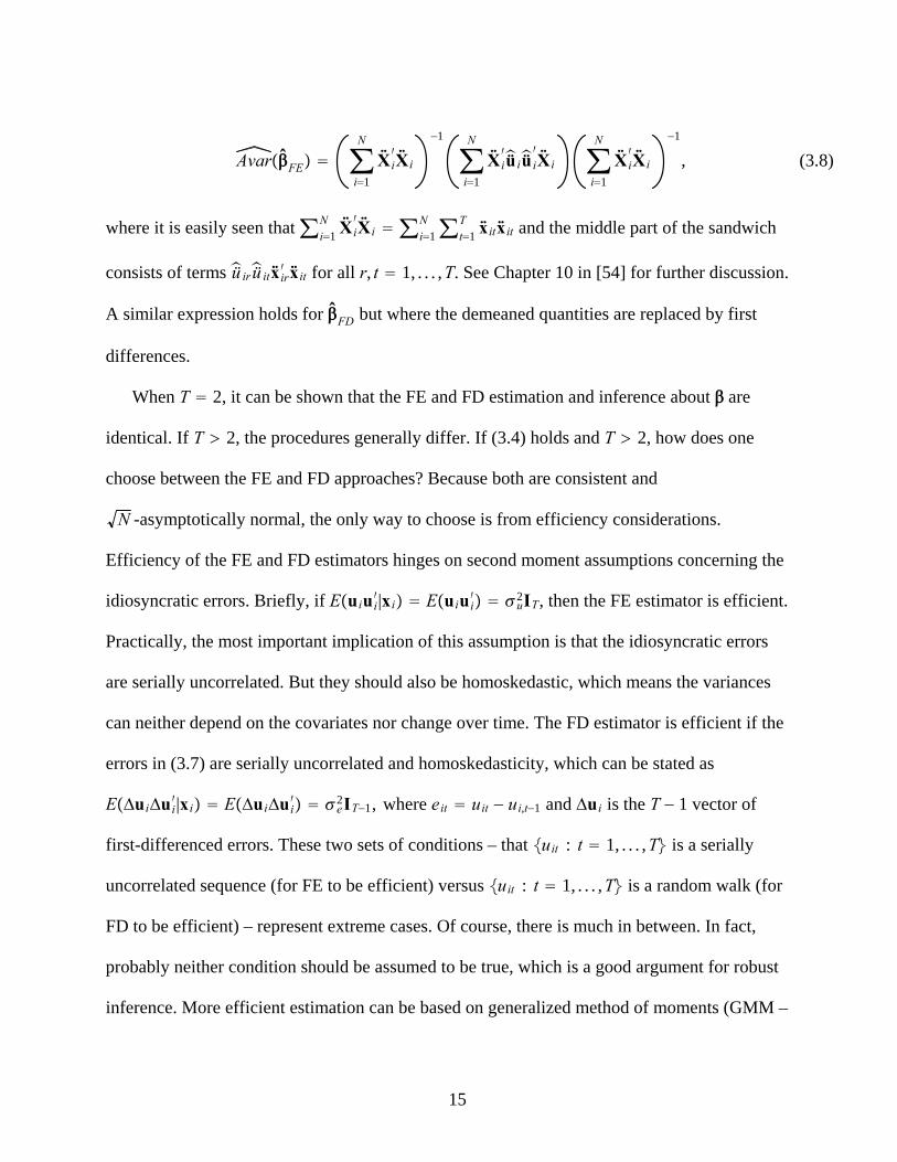
AvarFE ∑i1

N

Xi′Xi

−1

∑i1

N

Xi′ü iü i′Xi ∑

i1

N

Xi′Xi

−1

, (3.8)

where it is easily seen that∑ i1N Xi

′Xi ∑ i1

N ∑ t1T xitxit and the middle part of the sandwich

consists of termsüirüitxir′ xit for all r, t 1, . . . ,T. See Chapter 10 in [54] for further discussion.

A similar expression holds for FD but where the demeaned quantities are replaced by first

differences.

When T 2, it can be shown that the FE and FD estimation and inference about are

identical. If T 2, the procedures generally differ. If (3.4) holds and T 2, how does one

choose between the FE and FD approaches? Because both are consistent and

N -asymptotically normal, the only way to choose is from efficiency considerations.

Efficiency of the FE and FD estimators hinges on second moment assumptions concerning the

idiosyncratic errors. Briefly, if Euiui′|xi Euiui′ u2IT, then the FE estimator is efficient.

Practically, the most important implication of this assumption is that the idiosyncratic errors

are serially uncorrelated. But they should also be homoskedastic, which means the variances

can neither depend on the covariates nor change over time. The FD estimator is efficient if the

errors in (3.7) are serially uncorrelated and homoskedasticity, which can be stated as

EΔuiΔui′|xi EΔuiΔui′ e2IT−1, where eit uit − ui,t−1 and Δui is the T − 1 vector of

first-differenced errors. These two sets of conditions – that uit : t 1, . . . ,T is a serially

uncorrelated sequence (for FE to be efficient) versus uit : t 1, . . . ,T is a random walk (for

FD to be efficient) – represent extreme cases. Of course, there is much in between. In fact,

probably neither condition should be assumed to be true, which is a good argument for robust

inference. More efficient estimation can be based on generalized method of moments (GMM –

15

see Chapter 8 in [54] – or minimum distance estimation, as in [16]).

It is good practice to compute both FE and FD estimates to see if they differ in substantive

ways. It is also helpful to have a formal test of the strict exogeneity assumption that is easily

computable and that maintains only strict exogeneity under the null – in particular, that takes

no stand on whether the FE or FD estimator is asymptotically efficient. Because lags of

covariates can always be included in a model, the primary violation of (3.4) that is of interest is

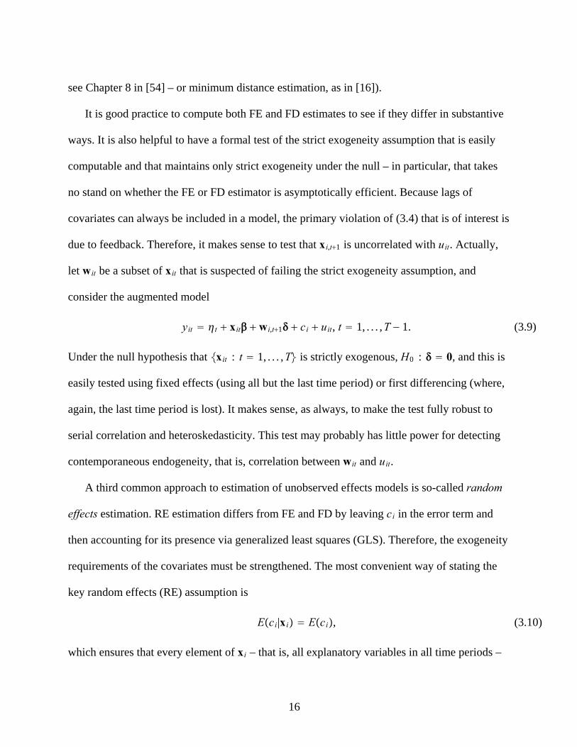
due to feedback. Therefore, it makes sense to test that xi,t1 is uncorrelated with uit. Actually,

let wit be a subset of xit that is suspected of failing the strict exogeneity assumption, and

consider the augmented model

yit t xit wi,t1 ci uit, t 1, . . . ,T − 1. (3.9)

Under the null hypothesis that xit : t 1, . . . ,T is strictly exogenous, H0 : 0, and this is

easily tested using fixed effects (using all but the last time period) or first differencing (where,

again, the last time period is lost). It makes sense, as always, to make the test fully robust to

serial correlation and heteroskedasticity. This test may probably has little power for detecting

contemporaneous endogeneity, that is, correlation between wit and uit.

A third common approach to estimation of unobserved effects models is so-called random

effects estimation. RE estimation differs from FE and FD by leaving ci in the error term and

then accounting for its presence via generalized least squares (GLS). Therefore, the exogeneity

requirements of the covariates must be strengthened. The most convenient way of stating the

key random effects (RE) assumption is

Eci|xi Eci, (3.10)

which ensures that every element of xi – that is, all explanatory variables in all time periods –

16

is uncorrelated with ci. Together with (3.4), (3.10) implies

Evit|xi 0, t 1, . . . ,T, (3.11)

where vit ci uit is the composite error. Condition (3.11) is the key condition for general

least squares methods that exploit serial correlation in vit to be consistent (although zero

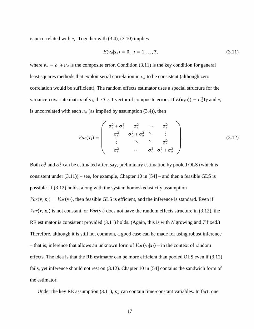
correlation would be sufficient). The random effects estimator uses a special structure for the

variance-covariate matrix of vi, the T 1 vector of composite errors. If Euiui′ u2IT and ci

is uncorrelated with each uit (as implied by assumption (3.4)), then

Varvi

c2 u2 c2 c2

c2 c2 u2

c2

c2 c2 c2 u2

. (3.12)

Both c2 and u2 can be estimated after, say, preliminary estimation by pooled OLS (which is

consistent under (3.11)) – see, for example, Chapter 10 in [54] – and then a feasible GLS is

possible. If (3.12) holds, along with the system homoskedasticity assumption

Varvi|xi Varvi, then feasible GLS is efficient, and the inference is standard. Even if

Varvi|xi is not constant, or Varvi does not have the random effects structure in (3.12), the

RE estimator is consistent provided (3.11) holds. (Again, this is with N growing and T fixed.)

Therefore, although it is still not common, a good case can be made for using robust inference

– that is, inference that allows an unknown form of Varvi|xi – in the context of random

effects. The idea is that the RE estimator can be more efficient than pooled OLS even if (3.12)

fails, yet inference should not rest on (3.12). Chapter 10 in [54] contains the sandwich form of

the estimator.

Under the key RE assumption (3.11), xit can contain time-constant variables. In fact, one

17

way to ensure that the omitted factors are uncorrelated with the key covariates is to include a

rich set of time-constant controls in xit. RE estimation is most convincing when many good

time-constant controls are available. In some applications of RE, the key variable of interest

does not change over time, which is why FE and FD cannot be used. (Methods proposed in

[25] can be used when some covariates are correlated with ci, but enough others are assumed

to be uncorrelated with ci.)

Rather than eliminate ci using the FE or FD transformation, or assuming (3.10) and using

GLS, a different approach is to explicitly model the correlation between ci and xi. A general

approach is to write

ci xi ai,

Eai 0 and Exi′ai 0,

(3.13)

(3.14)

where is a TK 1vector of parameters. Equations (3.13) and (3.14) are definitional, and

simply define the population linear regression of ci on the entire set of covariates, xi. This

representation is due to [16], and is an example of a correlated random effects (CRE) model.

The uncorrelated random effects model occurs when 0.

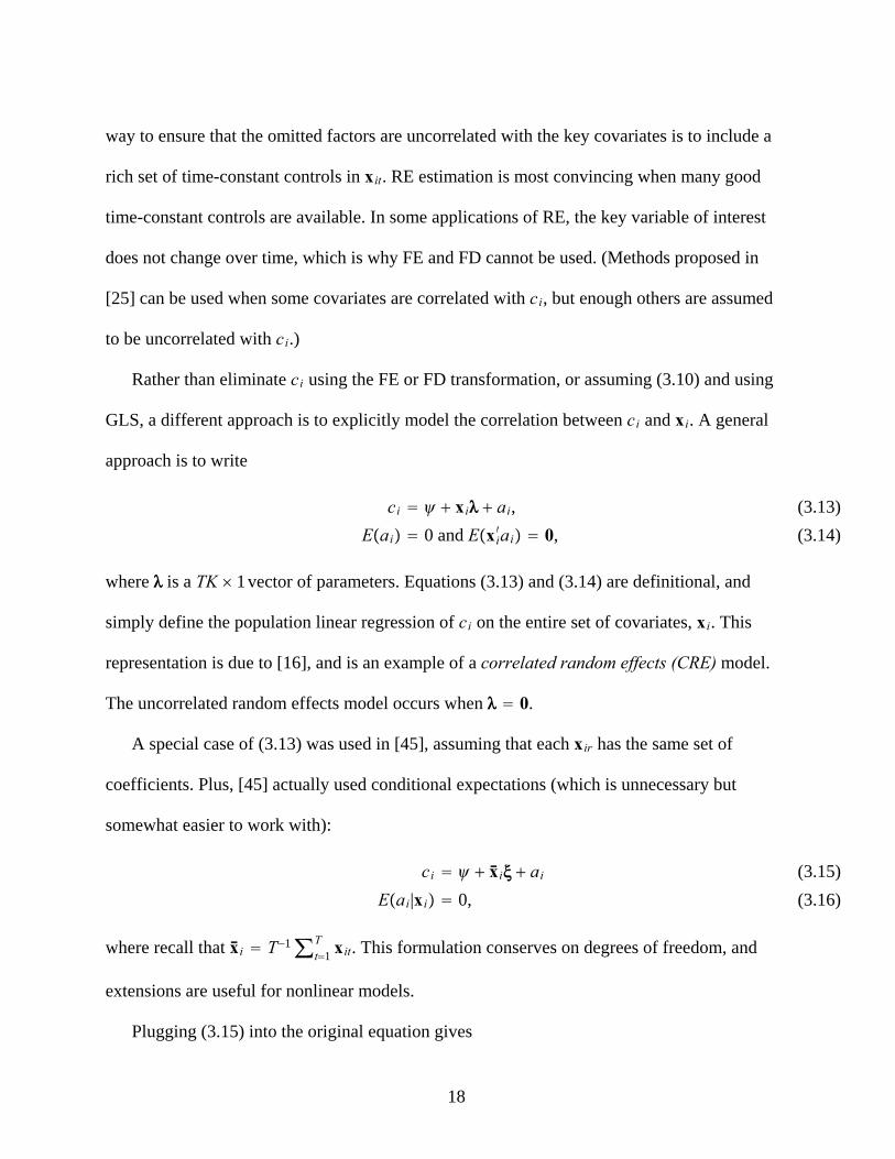
A special case of (3.13) was used in [45], assuming that each xir has the same set of

coefficients. Plus, [45] actually used conditional expectations (which is unnecessary but

somewhat easier to work with):

ci xi aiEai|xi 0,

(3.15)

(3.16)

where recall that xi T−1∑ t1T xit. This formulation conserves on degrees of freedom, and

extensions are useful for nonlinear models.

Plugging (3.15) into the original equation gives

18

yit t xit xi ai uit, (3.17)

where is absorbed into the time intercepts.) The composite error ai uit satisfies

Eai uit|xi 0, and so pooled OLS or random effects applied to (3.17) produces consistent,

N -asymptotically normal estimators of all parameters, including . In fact, if the original

model satisfies the second moments ideal for random effects, then so does (3.17). Interesting,

both pooled OLS and RE applied to (3.17) produce the fixed effects estimate of (and the t).

Therefore, the FE estimator can be derived from a correlated random effects model.

(Somewhat surprisingly, the same algebraic equivalence holds using Chamberlain’s more

flexible device. Of course, the pooled OLS estimator is not generally efficient, and [16] shows

how to obtain the efficient minimum distance estimator. See also Chapter 11 in [54].)

One advantage of equation (3.17) is that it provides another interpretation of the FE

estimate: it is obtained by holding fixed the time averages when obtaining the partial effects of

each xitj. This results in a more convincing analysis than not controlling for systematic

differences in the levels of the covariates across i.

Equation (3.17) has other advantages over just using the time-demeaned data in pooled

OLS: time-constant variables can be included in (3.17), and the resulting equation gives a

simple, robust way of testing whether the time-varying covariates are uncorrelated with It is

helpful to write the original equation as

yit gt zi wit ci uit, t 1, . . . ,T, (3.18)

where gt is typically a vector of time period dummies but could instead include other variables

that change only over time, including linear or quadratic trends, zi is a vector of time-constant

variables, and wit contains elements that vary across i and t. It is clear that, in comparing FE to

19

RE estimation, can play no role because it cannot be estimated by FE. What is less clear, but

also true, is that the coefficients on the aggregate time variables, , cannot be included in any

comparison, either. Only the M 1 estimates of , say FE and RE, can be compared. If FE

and RE are included, the asymptotic variance matrix of the difference in estimators has a

nonsingularity in the asymptotic variance matrix. (In fact, RE and FE estimation only with

aggregate time variables are identical.) The Mundlak equation is now

yit gt zi wit wi ai uit, t 1, . . . ,T, (3.19)

where the intercept is absorbed into gt. A test of the key RE assumption is H0 : 0 is

obtained by estimating (3.19) by RE, and this equation makes it clear thereM restrictions to

test. This test was described in [45] and [5] proposed the robust version. The original test based

directly on comparing the RE and FE estimators, as proposed in [24], it more difficult to

compute and not robust because it maintains that the RE estimator is efficient under the null.

The model in (3.19) gives estimates of the coefficients on the time-constant variables zi.

Generally, these can be given a causal interpretation only if

Eci|wi,zi Eci|wi wi, (3.20)

where the first equality is the important one. In other words, zi is uncorrelated with ci once the

time-varying covariates are controlled for. This assumption is too strong in many applications,

but one still might want to include time-constant covariates.

Before leaving this subsection, it is worth point out that generalized least squares methods

with an unrestricted variance-covariance matrix can be applied to every estimating equation

just presented. For example, after eliminating ci by removing the time averages, the resulting

vector of errors, üi, can have an unrestricted variance matrix. (Of course, there is no guarantee

20

that this matrix is the same as the variance matrix conditional on the matrix of time-demeaned

regressors, Xi.) The only glitch in practice is that Varüi has rank T − 1, not T. As it turns out,

GLS with an unrestricted variance matrix for the original error vector, ui, can be implemented

on the time-demeaned equation with any of the T time periods dropped. The so-called fixed

effects GLS estimates are invariant to whichever equation is dropped. See [40] or [36] for

further discussion. The initial estimator used to estimate the variance covariance matrix would

probably be the usual FE estimator (applied to all time periods).

Feasible GLS can be applied directly the first differenced equation, too. It can also be

applied to (3.19), allowing the composite errors ai uit, t 1, . . . ,T, to have an unrestricted

variance-covariance matrix. In all cases, the assumption that the conditional variance matrix

equals the unconditional variance can fail, and so one should use fully robust inference even

after using FGLS. Chapter 10 in [54] provides further discussion. Such options are widely

available in software, sometimes under the rubric of generalized estimating equations (GEE).

See, for example, [42].

3.2. Models with Heterogeneous Slopes

The basic model described in the previous subsection introduces a single source of

heterogeneity in the additive effect, ci. The form of the model implies that the partial effects of

the covariates depend on a fixed set of population values (and possibly other unobserved

covariates if interactions are included in xit). It seems natural to extend the model to allow

interactions between the observed covariates and time-constant, unobserved heterogeneity:

yit ci xitbi uitEuit|xi,ci,bi 0, t 1, . . . ,T,

(3.21)

(3.22)

where bi is K 1. With small T, one cannot precisely estimate bi. Instead, attention usually

21

focuses on the average partial effect (APE) or population averaged effect (PAE). In (3.21), the

vector of APEs is ≡ Ebi, the K 1 vector of means. In this formulation, aggregate time

effects are in xit. This model is sometimes called a correlated random slopes model – which

means the slopes are allowed to be correlated with the covariates.

Generally, allowing ci,bi and xi to be arbitrarily correlated requires T K 1 – see [55].

With a small number of time periods and even a modest number of regressors, this condition

often fails in practice. Chapter 11 in [54] discusses how to allow only a subset of coefficients

to be unit specific. Of interest here is the question: if the usual FE estimator is applied – that is,

ignoring the unit-specific slopes bi – does this ever consistently estimate the APEs in ? In

addition to the usual rank condition and the strict exogeneity assumption (3.22), [55] shows

that a simple sufficient condition is

Ebi|xit Ebi , t 1, . . . ,T. (3.23)

Importantly, condition (3.23) allows the slopes, bi, to be correlated with the regressors xit

through permanent components. It rules out correlation between idiosyncratic movements in xit

and bi. For example, suppose the covariates can be decomposed as xit fi r it, t 1, . . . ,T.

Then (3.23) holds if Ebi|r i1,r i2, . . . ,r iT Ebi. In other words, bi is allowed to be arbitrarily

correlated with the permanent component, fi. Condition (3.23) is similar in spirit to the key

assumption in [45] for the intercept ci: the correlation between the slopes bij and the entire

history xi1, . . . ,xiT is through the time averages, and not through deviations from the time

averages. If bi changes across i, ignoring it by using the usual FE estimator effectively puts

xitbi − in the error term, which induces heteroskedasticity and serial correlation in the

composite error even if the uit are homoskedastic and serially independent. The possible

presence of this term provides another argument for making inference with FE fully robust to

22

arbitrary conditional and unconditional second moments.

The (partial) robustness of FE to the presence of correlated random slopes extends to a

more general class of estimators that includes the usual fixed effects estimator. Write an

extension of the basic model as

yit gtai xitbi uit, t 1, . . . ,T, (3.24)

where gt is a set of deterministic functions of time. A leading case is gt 1, t, so that each

unit has its own time trend along with a level effect. (The resulting model is sometimes called

a random trend model.) Now, assume that the random coefficients, ai, are swept away be

regressing yit and xit each on gt for each i. The residuals, ÿit and xit, have had unit-specific

trends removed, but the bi are treated as constant in the estimation. The key condition for

consistently estimating can still be written as in (3.23), but now xit has had more features

removed at unit-specific level. When gt 1, t, each covariate has been demeaned within

each unit. Therefore, if xit fi hit r it, then bi can be arbitrarily correlated with fi,hi. Of

course, individually detrending the xit requires at least three time periods, and it decreases the

variation in xit compared with the usual FE estimator. Not surprisingly, increasing the

dimension of gt (subject to the restriction dimgt T), generally leads to less precision of the

estimator. See [55] for further discussion.

23

4. Sequentially Exogenous Regressors and Dynamic Models

The summary of models and estimators from Section 3 used the strict exogeneity

assumption Euit|xi,ci 0 for all t, and added an additional assumption for models with

correlated random slopes. As discussed in Section 3, strict exogeneity is not an especially

natural assumption. The contemporaneous exogeneity assumption Euit|xit,ci 0 is

attractive, but the parameters are not identified. In this section, a middle ground between these

assumptions, which has been called a sequential exogeneity assumption, is used. But first, it is

helpful to understand properties of the FE and FD estimators when strict exogeneity fails.

4.1. Behavior of Estimators without Strict Exogeneity

Both the FE and FD estimators are inconsistent (with fixed T, N → ) without the strict

exogeneity assumption stated in equation (3.4). But it is also pretty well known that, at least

under certain assumptions, the FE estimator can be expected to have less “bias” for larger T.

Under the contemporaneous exogeneity assumption (3.2) and the assumption that the data

series xit,uit : t 1, . . . ,T is “weakly dependent” – in time series parlance, “integrated of

order zero,” or I(0) – then it can be shown that

plim FE OT−1

plim FD O1;

(4.1)

(4.2)

see Chapter 11 in [54]. In some very special cases, such as the simple AR(1) model discussed

below, the “bias” terms can be calculated, but not generally.

Interestingly, the same results can be shown if xit : t 1, . . . ,T has unit roots as long as

uit is I(0) and contemporaneous exogeneity holds. However, there is a catch: if uit is I(1) –

so that the time series version of the “model” would be a spurious regression (yit and xit are not

24

“cointegrated”), then (4.1) is no longer true. On the other hand, first differencing means any

unit roots are eliminated and so there is little possibility of a spurious regression. The bottom

line is that using “large T” approximations such as those in (4.1) and (4.2) to choose between

FE over FD obligates one to take the time series properties of the panel data seriously; one

must recognize the possibility that the FE estimation is essentially a spurious regression.

4.2. Consistent Estimation under Sequential Exogeneity

Because both the FE and FD estimators are inconsistent for fixed T, it makes sense to

search for estimators that are consistent for fixed T. A natural specification for dynamic panel

data models, and one that allows consistent estimation under certain assumptions, is

Eyit|xi1, . . . ,xit,ci Eyit|xit,ci t xit ci, (4.3)

which says that xit contains enough lags so that further lags of variables are not needed. When

the model is written in error form, (4.3) is the same as

Euit|xi1, . . . ,xit,ci 0, t 1,2, . . . ,T. (4.4)

Under (4.4), the covariates xit : t 1, . . . ,T are said to be sequentially exogenous

conditional on ci. Some estimation methods are motivated by a weaker version of (4.4),

namely,

Exis′ uit 0, s 1, . . . , t, t 1, . . . ,T, (4.5)

but (4.4) is natural in most applications.

Assumption (4.4) is appealing in that it allows for finite distributed lag models as well as

models with lagged dependent variables. For example, the finite distributed lag model

yit t zit0 zi,t−11 . . .zi,t−LL ci uit (4.6)

allows the elements of zit to have effects up to L time periods after a change. With

25

xit zit,zi,t−1, . . . ,zi,t−L, Assumption (4.4) implies

Eyit|zit,zi,t−1,zi,t−2, . . . ,ci Eyit|zit,zi,t−1,zi,t−2,ci t zit0 zi,t−11 . . .zi,t−LL ci, (4.7)

which means that the distributed lag dynamics are captured by L lags. The important difference

with the strict exogeneity assumption is that sequential exogeneity allows feedback from uit to

zir for r t.

How can (4.4) be used for estimation? The FD transformation is natural because of the

sequential nature of the restrictions. In particular, write the FD equation as

Δyit Δxit Δuit, t 2, . . . ,T. (4.8)

Then, under (4.5),

Exis′ Δuit 0, s 1, . . . , t − 1; t 2, . . . ,T, (4.9)

which means any xis with s t can be used as an instrument for the time t FD equation. An

efficient estimator that uses (4.9) is obtained by stacking the FD equations as

Δyi ΔXi Δui, (4.10)

where Δyi Δyi2,Δyi3, . . . ,ΔyiT ′ is the T − 1 1 vector of first differences and ΔXi is the

T − 1 K matrix of differences on the regressors. (Time period dummies are absorbed into

xit for notational simplicity.) To apply a system estimation method to (4.10), define

xito ≡ xi1,xi2, . . . ,xit, (4.11)

which means the valid instruments at time t are in xi,t−1o (minus redundancies, of course). The

matrix of instruments to apply to (4.10) is

Wi diagxi1o ,xi2o , . . . ,xi,T−1

o , (4.12)

which has T − 1 rows and a large number of columns. Because of sequential exogeneity, the

26

number of valid instruments increases with t.

GivenWi, it is routine to apply generalized method of moments estimation, as summarized

in [26] and [54]. A simpler strategy is available that can be used for comparison or as the

first-stage estimator in computing the optimal weighting matrix. First, estimate a reduced form

for Δxit separately for each t. In other words, at time t, run the regression Δxit on xi,t−1o ,

i 1, . . . ,N, and obtain the fitted values, Δxit. Of course, the fitted values are all 1 K vectors

for each t, even though the number of available instruments grows with t. Then, estimate the

FD equation (4.8) by pooled IV using Δxit as instruments (not regressors). It is simple to obtain

robust standard errors and test statistics from such a procedure because the first stage

estimation to obtain the instruments can be ignored (asymptotically, of course).

One potential problem with estimating the FD equation using IVs that are simply lags of xit

is that changes in variables over time are often difficult to predict. In other words, Δxit might

have little correlation with xi,t−1o . This is an example of the so-called “weak instruments”

problem, which can cause the statistical properties of the IV estimators to be poor and the usual

asymptotic inference misleading. Identification is lost entirely if xit t xi,t−1 qit, where

Eqit|xi,t−1, . . . ,xi1 0 – that is, the elements of xit are random walks with drift. Then, then

EΔxit|xi,t−1, . . . ,xi1 0, and the rank condition for IV estimation fails. Of course, if some

elements of xit are strictly exogenous, then their changes act as their own instruments.

Nevertheless, typically at least one element of xit is suspected of failing strict exogeneity,

otherwise standard FE or FD would be used.

In situations where simple estimators that impose few assumptions are too imprecise to be

useful, sometimes one is willing to improve estimation of by adding more assumptions. How

can this be done in the panel data case under sequential exogeneity? There are two common

27

approaches. First, the sequential exogeneity condition can be strengthened to the assumption

that the conditional mean model is dynamically complete, which can be written in terms of the

errors as

Euit|xit,yi,t−1xi,t−1, . . . ,yi1,xi1,ci 0, t 1, . . . ,T. (4.13)

Clearly, (4.13) implies (4.4). Dynamic completeness is neither stronger nor weaker than strict

exogeneity, because the latter includes the entire history of the covariates while (4.13)

conditions only on current and past xit. Dynamic completeness is natural when xit contains

lagged dependent variables, because it basically means enough lags have been included to

capture all of the dynamics. It is often too restrictive in finite distributed lag models such as

(4.6), where (4.13) would imply

Eyit|zit,yi,t−1zi,t−1, . . . ,yi1,zi1,ci Eyit|zit,zi,t−1, . . . ,zi−L,ci, t 1, . . . ,T, (4.14)

which puts strong restrictions on the fully dynamic conditional mean: values yir, r ≤ t − 1, do

not help to predict yit once zit,zi,t−1, . . . are controlled for. FDLs are of interest even if (4.14)

does not hold. Imposing (4.13) in FDLs implies that the idiosyncratic errors must be serially

uncorrelated, something that is often violated in FDLs.

Dynamic completeness is natural in a model such as

yit yi,t−1 zit0 zi,t−11 ci uit. (4.15)

Usually – although there are exceptions – (4.15) is supposed to represent the conditional mean

Eyit|zit,yi,t−1zi,t−1, . . . ,yi1,zi1,ci, and then the issue is whether one lag of yit and zit suffice to

capture the dynamics.

Regardless of what is contained in xit, assumption (4.13) implies some additional moment

conditions that can be used to estimate . The extra moment conditions, first proposed in [2] in

28

the context of the AR(1) unobserved effects model, can be written as

EΔyi,t−1 − Δxi,t−1 ′yit − xit 0, t 3, . . . ,T; (4.16)

see also [9]. The conditions can be used in conjunction with those in equation (4.9) in a method

of moments estimation method. In addition to imposing dynamic completeness, the moment

conditions in (4.16) are nonlinear in parameters, which makes them more difficult to

implement than just using (4.9). Nevertheless, the simulation evidence in [2] for the AR(1)

model shows that (4.16) can help considerably when the coefficient is large.

[7] suggested a different set of restrictions,

CovΔxit′ ,ci 0, t 2, . . . ,T. (4.17)

Interestingly, this assumption is very similar in spirit to assumption (3.23), except that it is in

terms of the first difference of the covariates, not the time-demeaned covariates. Condition

(4.17) generates moment conditions in the levels of equation,

EΔxit′ yit − − xit 0, t 2, . . . ,T, (4.18)

where allows for a nonzero mean for ci. [10] applies these moment conditions, along with

the usual conditions in (4.9), to estimate firm-level production functions. Because of

persistence in the data, they find the moments in (4.9) are not especially informative for

estimating the parameters, whereas (4.18) along with (4.9) are. Of course, (4.18) is an extra set

of assumptions.

The previous discussion can be applied to the AR(1) model, which has received much

attention. In its simplest form the model is

yit yi,t−1 ci uit, t 1, . . . ,T, (4.19)

so that, by convention, the first observation on y is at t 0. The minimal assumptions imposed

29

are

Eyisuit 0, s 0, . . . , t − 1, t 1, . . . ,T, (4.20)

in which case the available instruments at time t are wit yi0, . . . ,yi,t−2 in the FD equation

Δyit Δyi,t−1 Δuit, t 2, . . . ,T. (4.21)

Written in terms of the parameters and observed data, the moment conditions are

EyisΔyit − Δyi,t−1 0, s 0, . . . , t − 2, t 2, . . . ,T. (4.22)

[4] proposed pooled IV estimation of the FD equation with the single instrument yi,t−2 (in

which case all T − 1 periods can be used) or Δyi,t−2 (in which case only T − 2 periods can be

used). A better approach is pooled IV where T − 1 separate reduced forms are estimated for

Δyi,t−1 as a linear function of yi0, . . . ,yi,t−2. The fitted values Δyi,t−1, can be used as the

instruments in (4.21) in a pooled IV estimation. Of course, standard errors and inference

should be made robust to the MA(1) serial correlation in Δuit. [6] suggested full GMM

estimation using all of the available instruments yi0, . . . ,yi,t−2, and this estimator uses the

conditions in (4.20) efficiently.

Under the dynamic completeness assumption

Euit|yi,t−1,yi,t−2, . . . ,yi0,ci 0, (4.23)

the extra moment conditions in [2] become

EΔyi,t−1 − Δyi,t−2yit − yi,t−1 0, t 3, . . . ,T. (4.24)

[10] noted that if the condition

CovΔyi1,ci Covyi1 − yi0,ci 0 (4.25)

is added to (4.23) then the combined set of moment conditions becomes

30

EΔyi,t−1yit − − yi,t−1 0, t 2, . . . ,T, (4.26)

which can be added to the usual moment conditions (4.22). Conditions (4.22) and (4.26)

combined are attractive because they are linear in the parameters, and they can produce much

more precise estimates than just using (4.22).

As discussed in [10], condition (4.25) can be interpreted as a restriction on the initial

condition, yi0, and the steady state. When || 1, the steady state of the process is ci/1 − .

Then, it can be shown that (4.25) holds if the deviation of yi0 from its steady state is

uncorrelated with ci. Statistically, this condition becomes more useful as approaches one, but

this is when the existence of a steady state is most in doubt. [21] shows theoretically that such

restrictions can greatly increase the information about .

Other approaches to dynamic models are based on maximum likelihood estimation.

Approaches that condition on the initial condition yi0, suggested by [15], [13], and [10], seem

especially attractive. Under normality assumptions, maximum likelihood conditional on yi0 is

tractable.

If some strictly exogenous variables are added to the AR(1) model, then it is easiest to use

IV methods on the FD equation, namely,

Δyit Δyi,t−1 Δzit Δuit, t 1, . . . ,T. (4.27)

The available instruments (in addition to time period dummies) are zi,yi,t−2, . . . ,yi0, and the

extra conditions (4.18) can be used, too. If sequentially exogenous variables, say hit, are added,

then hi,t−1, . . . ,hi1 would be added to the list of instruments (and Δhit would appear in the

equation).

31

5. Unbalanced Panel Data Sets

The previous sections considered estimation of models using balanced panel data sets,

where each unit is observed in each time period. Often, especially with data at the individual,

family, or firm level, data are missing in some time periods – that is, the panel data set is

unbalanced. Standard methods, such as fixed effects, can often be applied to produce

consistent estimators, and most software packages that have built-in panel data routines

typically allow unbalanced panels. However, determining whether applying standard methods

to the unbalanced panel produces consistent estimators requires knowing something about the

mechanism generating the missing data.

Methods based on removing the unobserved effect warrant special attention, as they allow

some nonrandomness in the sample selection. Let t 1, . . . ,T denote the time periods for

which data can exist for each unit from the population, and again consider the model

yit t xit ci uit, t 1, . . . ,T. (5.1)

It is helpful to have, for each i and t, a binary selection variable, sit, equal to one of the data for

unit i in time t can be used, and zero otherwise. For concreteness, consider the case where time

averages are removed to eliminate ci, but where the averages necessarily only include the

sit 1 observations. Let ÿit yit − Ti−1∑r1T siryir and xit xit − Ti−1∑r1

T sirxir be the

time-demeaned quantities using the observed time periods for unit i, where Ti ∑ t1T sit is the

number of time periods observed for unit i – properly viewed as a random variable. The fixed

effects estimator on the unbalanced panel can be expressed as

32

FE N−1∑i1

N

∑t1

T

sitxit′ xit

−1

N−1∑i1

N

∑t1

T

sitxit′ ÿit

N−1∑i1

N

∑t1

T

sitxit′ xit

−1

N−1∑i1

N

∑t1

T

sitxit′ uit .

(5.2)

With fixed T and N → asymptotics, the key condition for consistency is

∑t1

T

Esitxit′ uit 0. (5.3)

In evaluating (5.3), it is important to remember that xit depends on xi1, . . . ,xiT, si1, . . . , siT, and

in a nonlinear way. Therefore, it is not sufficient to assume xir, sir are uncorrelated with uit

for all r and t. A condition that is sufficient for (5.3) is

Euit|xi1, . . . ,xiT, si1, . . . , siT,ci 0, t 1, . . . ,T. (5.4)

Importantly, (5.4) allows arbitrary correlation between the heterogeneity, ci, and selection, sit,

in any time period t. In other words, some units are allowed to be more likely to be in or out of

the sample in any time period, and these probabilities can change across t. But (5.4) rules out

some important kinds of sample selection. For example, selection at time t, sit, cannot be

correlated with the idiosyncratic error at time t, uit. Further, feedback is not allowed: in affect,

like the covariates, selection must be strictly exogenous conditional on ci.

Testing for no feedback into selection is easy in the context of FE estimation. Under (5.4),

si,t1 and uit should be uncorrelated. Therefore, si,t1 can be added to the FE estimation on the

unbalanced panel – where the last time period is lost for all observations – and a t test can be

used to determine significance. A rejection means (5.4) is false. Because serial correlation and

heteroskedasticity are always a possibility, the t test should be made fully robust.

Contemporaneous selection bias – that is, correlation between sit and uit – is more difficult

33

to test. Chapter 17 in [54] summarizes how to derive tests and corrections by extending the

corrections in [27] (so-called “Heckman corrections”’) to panel data.

First differencing can be used on unbalanced panels, too, although straight first

differencing can result in many lost observations: a time period is used only if it is observed

along with the previous or next time period. FD is more useful in the case of attrition in panel

data, where a unit is observed until it drops out of the sample and never reappears. Then, if a

data point is observed at time t, it is also observed at time t − 1. Differencing can be combined

with the approach in [27] to solve bias due to attrition – at least under certain assumptions. See

Chapter 17 in [54].

Random effects methods can also be applied with unbalanced panels, but the assumptions

under which the RE estimator is consistent are stronger than for FE. In addition to (5.4), one

must assume selection is unrelated to ci. A natural assumption, that also imposes exogeneity on

the covariates with respect to ci, is

Eci|xi1, . . . ,xiT, si1, . . . , siT Eci. (5.5)

The only case beside randomly determined sample selection where (5.5) holds is when sit is

essentially a function of the observed covariates. Even in this case, (5.5) requires that the

unobserved heterogeneity is mean independent of the observed covariates – as in the typical

RE analysis on balanced panel.

34

6. Nonlinear Models

Nonlinear panel data models are considerably more difficult to interpret and estimate than

linear models. Key issues concern how the unobserved heterogeneity appears in the model and

how one accounts for that heterogeneity in summarizing the effects of the explanatory

variables on the response. Also, in some cases, conditional independence of the response is

used to identify certain parameters and quantities.

6.1. Basic Issues and Quantities of Interest

As in the linear case, the setup here is best suited for situations with small T and large N. In

particular, the asymptotic analysis underlying the discussion of estimation is with fixed T and

N → . Sampling is assumed to be random from the population. Unbalanced panels are

generally difficult to deal with because, except in special cases, the unobserved heterogeneity

cannot be completely eliminated in obtaining estimating equations. Consequently, methods

that model the conditional distribution of the heterogeneity conditional on the entire history of

the covariates – as we saw with the Chamberlain-Mundlak approach – are relied on heavily,

and such approaches are difficult when data are missing on the covariates for some time

periods. Therefore, this section considers only balanced panels. The discussion here takes the

response variable, yit, as a scalar for simplicity.

The starting point for nonlinear panel data models with unobserved heterogeneity is the

conditional distribution

Dyit|xit,c i, (6.1)

where c i is the unobserved heterogeneity for observation idrawn along with the observables.

Often there is a particular feature of this distribution, such as Eyit|xit,c i, or a conditional

35

median, that is of primary interest. Even focusing on the conditional mean raises some tricky

issues in models where c i does not appear in an additive or linear form. To be precise, let

Eyit|xit xt,c i c mtxt,c be the mean function. If xtj is continuous, then the partial

effect can be defined as

jxt,c ≡∂mtxt,c∂xtj

. (6.2)

For discrete (or continuous) variables, (6.2) can be replaced with discrete changes. Either way,

a key question is: How can one account for the unobserved c in (6.2)? In order to estimate

magnitudes of effects, sensible values of c need to be plugged into (6.2), which means

knowledge of at least some distributional features of c i is needed. For example, suppose

c Ec i is identified. Then the partial effect at the average (PEA),

jxt,c, (6.3)

can be identified if the regression function mt is identified. Given more information about the

distribution of c i, different quantiles can be inserted into (6.3), or a certain number of standard

deviations from the mean.

An alternative to plugging in specific values for c is to average the partial effects across the

distribution of c i:

APExt Ecijxt,c i, (6.4)

the so-called average partial effect (APE). The difference between (6.3) and (6.4) can be

nontrivial for nonlinear mean functions. The definition in (6.4) dates back at least to [17], and

is closely related to the notion of the average structural function (ASF), as introduced in [12].

The ASF is defined as

36

ASFxt Ecimtxt,c i. (6.5)

Assuming the derivative passes through the expectation results in (6.4); computing a discrete

change in the ASF always gives the corresponding APE. A useful feature of APEs is that they

can be compared across models, where the functional form of the mean or the distribution of

the heterogeneity can be different. In particular, APEs in general nonlinear models are

comparable to the estimated coefficients in a standard linear model.

Average partial effects are not always identified, even when parameters are.

Semi-parametric panel data methods that are silent about the distribution of c i, unconditionally

or conditional on xi1, . . . ,xiT, cannot generally deliver estimates of APEs, essentially by

design. Instead, an index structure is usually imposed so that parameters can be consistently

estimated. A common setup with scalar heterogeneity is

mtxt,c Gxt c, (6.6)

where, say, G is strictly increasing and continuously differentiable. The partial effects are

proportional to the parameters:

jxt,c jgxt c, (6.7)

where g is the derivative of G. Therefore, if j is identified, then so is the sign of the

partial effect, and even the relative effects of any two continuous variables: the ratio of partial

effects for xtj and xth is j/h. However, even if G is specified (the common case), the

magnitude of the effect evidently cannot be estimated without making assumptions about the

distribution of ci; otherwise, the term Egxt ci cannot generally be estimated. The probit

example below shows how the APEs can be estimated in index models under distributional

assumptions for ci..

37

The previous discussion holds regardless of the exogeneity assumptions on the covariates.

For example, the definition of the APE for a continuous variable holds whether xt contains

lagged dependent variables or only contemporaneous variables. However, approaches for

estimating the parameters and the APEs depend critically on exogeneity assumptions.

6.2. Exogeneity Assumptions on the Covariates

As in the case of linear models, it is not nearly enough to simply specify a model for the

conditional distribution of interest, Dyit|xit,c i, or some feature of it, in order to estimate

parameters and partial effects. This section offers two exogeneity assumptions on the

covariates that are more restrictive versions of the linear model assumptions.

It is easiest to deal with estimation under a strict exogeneity assumption. The most useful

definition of strict exogeneity for nonlinear panel data models is

Dyit|xi1, . . . ,xiT,c i Dyit|xit,c i, (6.8)

which means that xir, r ≠ t, does not appear in the conditional distribution of yit once xit and c i

have been counted for. [17] labeled (6.8) strict exogeneity conditional on the unobserved

effects c i. Sometimes, a conditional mean version is sufficient:

Eyit|xi1, . . . ,xiT,c i Eyit|xit,c i, (6.9)

which already played a role in linear models. Assumption (6.8), or its conditional mean

version, are less restrictive than if c i is not in the conditioning set, as discussed in [17]. Indeed,

it is easy to see that, if (6.8) holds and Dc i|xi depends on xi, then strict exogeneity without

conditioning on c i, Dyit|xi1, . . . ,xiT Dyit|xit, cannot hold. Unfortunately, both (6.8) and

(6.9) rule out lagged dependent variables, as well as other situations where there may be

feedback from idiosyncratic changes in yit to future movements in xir, r t. Nevertheless, the

38

conditional strict exogeneity assumption underlies the most common estimation methods for

nonlinear models.

More natural is sequential exogeneity conditional on the unobserved effects, which, in

terms of conditional distributions, is

Dyit|xi1, . . . ,xit,c i Dyit|xit,c i. (6.10)

Assumption (6.10) allows for lagged dependent variables and does not restrict feedback.

Unfortunately, (6.10) is substantially more difficult to work with than (6.8) for general

nonlinear models.

Because xit is conditioned on, neither (6.8) nor (6.10) allows for contemporaneous

endogeneity of xit as would arise with measurement error, time-varying omitted variables, or

simultaneous equations. This chapter does not treat such cases. See [37] for a recent summary.

6.3 Conditional Independence Assumption

The exogeneity conditions stated in Section 6.2 generally do not restrict the dependence in

the responses, yit : t 1, . . . ,T. Often, a conditional independence assumption is explicitly

imposed, which can be written generally as

Dyi1, . . . ,yiT|xi,c i t1

T

Dyit|xi,c i. (6.11)

Equation (6.11) simply means that, conditional on the entire history xit : t 1, . . . ,T and the

unobserved heterogeneity c i, the responses are independent across time. One way to think

about (6.11) is that time-varying unobservables are independent over time. Because (6.11)

conditions on xi, it is useful only in the context of the strict exogeneity assumption (6.8). Then,

conditional independence can be written as

39

Dyi1, . . . ,yiT|xi,c i t1

T

Dyit|xit,c i. (6.12)

Therefore, under strict exogeneity and conditional independence, the panel data modeling

exercise reduces to specifying a model for Dyit|xit,c i, and then determining how to treat the

unobserved heterogeneity, c i. In random effects and correlated RE frameworks, conditional

independence can play a critical role in being able to estimate the parameters and the

distribution of c i. As it turns out, conditional independence plays no role in estimating APEs

for a broad class of models. Before explaining how that works, the key issue of dependence

between the heterogeneity and covariates needs to be addressed.

6.4. Assumptions about the Unobserved Heterogeneity

For general nonlinear models, the random effects assumption is independence between c i

and xi xi1, . . . ,xiT:

Dc i|xi1, . . . ,xiT Dc i. (6.13)

Assumption (6.13) is very strong. To illustrate how strong it is, suppose that (6.13) is

combined with a model for the conditional mean, Eyit|xit xt,c i c mtxt,c. Without

any additional assumptions, the average partial effects are nonparametrically identified. In

particular, the APEs can be obtained directly from the conditional mean

rtxt ≡ Eyit|xit xt. (6.14)

(The argument is a simple application of the law of iterated expectations; it is discussed in

[55].) Nevertheless, (6.13) is still common in many applications, especially when the

explanatory variables of interest do not change over time.

As in the linear case, a correlated random effects (CRE) framework allows dependence

40

between c i and xi, but the dependence in restricted in some way. In a parametric setting, a

CRE approach involves specifying a distribution for Dc i|xi1, . . . ,xiT, as in [45], [15], [17],

and many subsequent authors; see, for example, [54] and [14]. For many models – see, for

example, Section 6.7 – one can allow Dc i|xi1, . . . ,xiT to depend on xi1, . . . ,xiT in a

“nonexchangeable” manner, that is, the distribution need not be symmetric on its conditioning

arguments. However, allowing nonexchangeability usually comes at the expense of potentially

restrictive distributional assumptions, such as homoskedastic normal with a linear conditional

mean. For estimating APEs, it is sufficient to assume, along with strict exogeneity,

Dc i|xi Dc i|xi, (6.15)

without specifying Dc i|xi or restricting any feature of this distribution. (See, for example, [3]

and [55].) As a practical matter, it makes sense to adopt (6.15) – or perhaps allow other

features of xit : t 1, . . . ,T – in a flexible parametric analysis.

Condition (6.15) still imposes restrictions on Dc i|xi. Ideally, as in the linear model, one

could estimate at least some features of interest without making any assumption about Dc i|xi.

Unfortunately, the scope for allowing unrestricted Dc i|xi is limited to special nonlinear

models, at least with small T. Allowing Dc i|xi to be unspecified is the hallmark of a “fixed

effects” analysis, but the label has not been used consistently. Often, fixed effects has been

used to describe a situation where the c i are treated as parameters to be estimated, along with

parameters that do not vary across i. Except in special cases or with large T, estimating the

unobserved heterogeneity is prone to an incidental parameters problem. Namely, using a fixed

T, N → framework, one cannot get consistent estimators of the c i, and the inconsistency in,

say, ĉ i, generally transmits itself to the parameters that do not vary with i. The incidental

parameters problem does not arise in estimating the coefficients in a linear model because

41

the estimator obtained by treating the ci as parameters to estimate is equivalent to pooled OLS

on the time-demeaned data – that is, the fixed effects estimator can be obtained by eliminating

the ci using the within transformation or estimating the ci along with . This occurrence is rare

in nonlinear models. Section 7 further discusses this issue, as there is much ongoing research

that attempts to reduce the asymptotic bias in nonlinear models.

The “fixed effects” label has also been applied to settings where the c i are not treated as

parameters to estimate; rather, the c i can be eliminated by conditioning on a sufficient statistic.

Let wi be a function of the observed data, xi,yi, such that

Dyi1, . . . ,yit|xi,c i,wi Dyi1, . . . ,yit|xi,wi. (6.16)

Then, provided the latter conditional distribution depends on the parameters of interest, and

can be derived or approximated from the original specification of Dyi1, . . . ,yit|xi,c i,

maximum likelihood methods can be used. Such an approach is also called conditional

maximum likelihood estimation (CMLE), where “conditional” refers to conditioning on a

function of yi. (In traditional treatments of MLE, conditioning on so-called “exogenous”

variables is usually implicit.) In most cases where the CMLE approach applies, the conditional

independence assumption (6.11) is maintained, although one conditional MLE is known to

have robustness properties: the so-called “fixed effects” Poisson estimator (see [52]).

6.5. Maximum Likelihood Estimation and Partial MLE

There are two common approaches to estimating the parameters in nonlinear, unobserved

effects panel data models when the explanatory variables are strictly exogenous. (A third

approach, generalized method of moments, is available in special cases but is not treated here.

See, for example, Chapter 19 in [54].) The first approach is full maximum likelihood

42

(conditional on the entire history of covariates). Most commonly, full MLE is applied under

the conditional independence assumption, although sometimes models are used that explicitly

allow dependence in Dyi1, . . . ,yiT|xi,c i. Assuming strict exogeneity, conditional

independence, a model for the density of yit given xit,c i [say, ftyt|xt,c;], and a model for

the density of c i given xi [say, hc|x;], the log likelihood for random draw i from the cross

section is

log t1

T

ftyit|xit,c; hc|xi;dc . (6.17)

This log-likelihood function “integrates out” the unobserved heterogeneity to obtain the joint

density of yi1, . . . ,yiT conditional on xi. In the most commonly applied models, including

logit, probit, Tobit, and various count models (such as the Poisson model), the log likelihood in

(6.17) identifies all of the parameters. Computation can be expensive but is typically tractable.

The main methodological drawback to the full MLE approach is that it is not robust to

violations of the conditional independence assumption, except for the linear model where

normal conditional distributions are used for yit and ci.

The partialMLE ignores temporal dependence in the responses when estimating the

parameters – at least when the parameters are identified. In particular, obtain the density of yit

given xi by integrating the marginal density for yit against the density for the heterogeneity:

gtyt|x;, ftyt|xt,c;hc|x;dc. (6.18)

The partial MLE (PMLE) (or pooled MLE) uses, for each i, the partial log likelihood

∑t1

T

loggtyit|xi;,. (6.19)

43

Because the partial MLE ignores the serial dependence caused by the presence of c i, it is

essentially never efficient. But in leading cases, such as probit, Tobit, and Poisson models,

gtyt|x;, has a simple form when hc|x; is chosen judiciously. Further, the PMLE is fully

robust to violations of (6.11). Inference is complicated by the neglected serial dependence, but

an appropriate adjustment to the asymptotic variance is easily obtained; see Chapter 13 in [54].

One complication with PMLE is that in the cases where it leads to a simple analysis

(probit, ordered probit, and Tobit, to name a few), not all of the parameters in and are

separately identified. The conditional independence assumption and the use of full MLE serves

to identify all parameters. Fortunately, the PMLE does identify the parameters that index the

average partial effects, a claim that will be verified for the probit model in Section 6.7.

6.6. Dynamic Models

General models with only sequentially exogenous variables are difficult to estimate. [8]

considered binary response models and [53] suggested a general strategy that requires

modeling the dynamic distribution of the variables that are not strictly exogenous.

Much more is known about the specific case where the model contains lagged dependent

variables along with strictly exogenous variables. The starting point is a model for the dynamic

distribution,

Dyit|zit,yi,t−1,zi,t−1. . . ,yi1,zi1,yi0,c i, t 1, . . . ,T, (6.20)

where zit are variables strictly exogenous (conditional on c i) in the sense that

Dyit|zi,yi,t−1,zi,t−1. . . ,yi1,zi1,yi0,c i Dyit|zit,yi,t−1,zi,t−1. . . ,yi1,zi1,yi0,c i, (6.21)

where zi is the entire history zit : t 1, . . . ,T.

In the leading case, (6.20) depends only on zit,yi,t−1,c i (although putting lags of strictly

44

exogenous variables only slightly changes the notation). Let ftyt|zt,yt−1,c; denote a model

for the conditional density, which depends on parameters . The joint density of yi1, . . . ,yiT

given yi0,zi,c i is

t1

T

ftyt|zt,yt−1,c;. (6.22)

The problem with using (6.22) for estimation is that, when it is turned into a log likelihood by

plugging in the “data,” c imust be inserted. Plus, the log likelihood depends on the initial

condition, yi0. Several approaches have been suggested to address these problems: (i) Treat the

c i as parameters to estimate (which results in an incidental parameters problem). (ii) Try to

estimate the parameters without specifying conditional or unconditional distributions for ci.

(This approach is available for very limited situations, and other restrictions are needed. And,

generally, one cannot estimate average partial effects.). (iii) Find, or, more practically,

approximate Dyi0|c i, zi and then model Dc i|zi. Integrating out c i gives the density for

Dyi0,yi1, . . . ,yiT|zi, which can be used in an MLE analysis (conditional on zi), (iv) Model

Dc i|yi0,zi. Then, integrate out c i conditional on yi0,zi to obtain the density for

Dyi1, . . . ,yiT|yi0,zi. Now, MLE is conditional on yi0,zi. As shown by [56], in some leading

cases – probit, ordered probit, Tobit, Poisson regression – there is a density hc|y0,z that

mixes with the density fy1, . . . ,yT|y0,z,c to produce a log-likelihood that is in a common

family and programmed in standard software packages.

If mtxt,c, is the mean function Eyt|xt,c, with xt zt,yt−1, then APEs are easy to

obtain. The average structural function is

ASFxt Ecimtxt,c i, E mtxt,c,hc|yi0,zi,dc |yi0,zi . (6.23)

45

The term inside the brackets, say rtxt,yi0,zi,, is available, at least in principle, because

mt and h have been specified. Often, they have simple forms, or they can be simulated. A

consistent estimator of the ASF is obtained by averaging out yi0,zi:

ASFxt N−1∑t1

T

rtxt,yi0,zi, , . (6.24)

Partial derivatives and differences with respect to elements of xt (which, remember, includes

functions of yt−1) can be computed. With large N and small T, the panel data bootstrap – where

resampling is carried out in the cross section so that every time period is kept when a unit i is

resampled – can be used for standard errors and inference. The properties of the nonparametric

bootstrap are standard in this setting because the resampling is carried out in the cross section.

6.7. Binary Response Models

Unobserved effects models – static and dynamic – have been estimated for various kinds of

response variables, including binary responses, ordered responses, count data, and corner

solutions. Most of the issues outlined above can be illustrated by binary response models,

which is the topic of this subsection.

The standard specification for the unobserved effects (UE) probit model is

Pyit 1|xit,ci xit ci, t 1, . . . ,T, (6.25)

where xit does not contain an overall intercept but would usually include time dummies, and ci

is the scalar heterogeneity. Without further assumptions, neither nor the APEs are identified.

The traditional RE probit model imposes a strong set of assumptions: strict exogeneity,

conditional independence, and independence between ci and xi with ci ~Normalc,c2.

Under these assumptions, and the parameters in the distribution of ci are identified and are

46

consistently estimated by full MLE (conditional on xi.

Under the strict exogeneity assumption (6.8), a correlated random effects version of the

model is obtained from the Chamberlain-Mundlak device under conditional normality:

ci xi ai,ai|xi ~Normal0,a2. (6.26)

The less restrictive version ci xi ai xi11 . . .xiTT ai can be used, but the

time average conserves on degrees of freedom.

As an example, suppose that yit is a binary variable indicating whether firm i in year t was

awarded at least one patent, and the key explanatory variable in xit is current and past spending

on research and development (R&D). It makes sense that R&D spending is correlated, at least

on average, with unobserved firm heterogeneity, and so a correlated random effects model

seems natural. Unfortunately, the strict exogeneity assumption might be problematical: it could

be that being awarded a patent in year t might affect future values of spending on R&D. Most

studies assume this is not the case, but one should be aware that, as in the linear case, the strict

exogeneity assumption imposes restrictions on economic behavior.

When the conditional independence assumption (6.11) is added to (6.25), strict exogeneity,

and (6.26), all parameters in (6.25) and (6.26) are identified (assuming that all elements of xit

are time-varying) and the parameters can be efficiently estimated by maximum likelihood

(conditional on xi). Afterwards, the mean of ci can be consistently estimated as

c N−1∑ i1N xi and the variance as c2

′N−1∑ i1

N xi′xi a2. Because ai is

normally distributed, ci is not normally distributed unless xi is. A normal approximation for

Dci gets better as T gets large. In any case, the estimated mean and standard deviation can be

used to plug in values of c that are a certain number of estimated standard deviations from c,

47

say c c or c 2c.

The APEs are identified from the ASF, which is consistently estimated by

ASFxt N−1∑i1

N

xta a xia (6.27)

where the “a” subscript means that a coefficient has been divided by 1 a21/2, for example,

a /1 a21/2. The derivatives or changes of ASFxt with respect to elements of xt can be

compared with fixed effects estimates from a linear model. Often, to obtain a single scale

factor, a further averaging across xit is done. The APEs computed from such averaging can be

compared to linear FE estimates.

The CRE probit model is an example of a model where the APEs are identified without the

conditional independence assumption. Without (6.11) – or any restriction on the joint

distribution – it can still be shown that

Pyit 1|xi xita a xia, (6.28)

which means a number of estimation approaches identify the scaled coefficients a, a, and a.

The estimates of these scaled coefficients can be inserted directly into (6.27). The unscaled

parameters and a2 are not separately identified, but in most cases this is a small price to pay

for relaxing the conditional independence assumption. Note that for determining directions of

effects and relative effects, a is just as useful as . Plus, it is a that appears in the APEs. The

partial effects at the mean value of ci are not identified.

Using pooled probit can be inefficient for estimating the scaled parameters. Full MLE, with

a specified correlation matrix for the T 1 vector ui, is possible in principle but difficult in

practice. An alternative approach, the generalized estimating equations (GEE) approach, can

48

be more efficient than pooled probit but just as robust in that only (6.28) is needed for

consistency. See [37] for a summary of how GEE – which is essentially the same as

multivariate weighted nonlinear least squares – applies to the CRE probit model.

A simple test of the strict exogeneity assumption is to add selected elements of xi,t1, say

wi,t1, to the model and computing a test of joint significance. Unless the full MLE is used, the

test should be made robust to serial dependence of unknown form. For example, as a test of

strict exogeneity of R&D spending when yit is a patent indicator, one can just include next

year’s value of R&D spending and compute a t test. In carrying out the test, the last time

period is lost for all firms.

Because there is nothing sacred about the standard model (6.25) under (6.26) – indeed,

these assumptions are potentially quite restrictive – it is natural to pursue other models and

assumptions. Even with (6.25) as the starting point, and under strict exogeneity, there are no

known ways of identifying parameters or partial effects without restricting Dci|xi.

Nevertheless, as mentioned in Section 6.4, there are nonparametric restrictions on Dci|xi that

do identify the APEs under strict exogeneity – even if (6.25) is dropped entirely. As shown in

[3], the restriction Dci|xi Dci|xi identifies the APEs. While fully nonparametric methods

can be used, some simple strategies are evident. For example, because the APEs can be

obtained from Dyit|xit, xi, it makes sense to apply flexible parametric models directly to this

distribution – without worrying about the original models for Dyit|xit,ci and Dci|xi.

As an example of this approach, a flexible parametric model, such as

Pyit 1|xit, xi t xit xi xi ⊗ xi xit ⊗ xi, (6.29)

might provide a reasonable approximation. The average structural function is estimated as

49

ASFxt N−1∑i1

N

t xt xi xi ⊗ xi xt ⊗ xi, (6.30)

where the estimates can come from pooled MLE, GEE, or a method of moments procedure.

The point is that extensions of the basic probit model such as (6.30) can provide considerable

flexibility and deliver good estimators of the APEs. The drawback is that one has to be willing

to abandon standard underlying models for Pyit 1|xit,ci and Dci|xi; in fact, it seems very

difficult to characterize models for these two features that would lead to an expression such as

(6.29).

An alternative model for the response probability is the logit model

Pyit 1|xit,ci xit ci, (6.31)

where z expz/1 expz. In cross section applications, researchers often find few

practical differences between (6.25) and (6.31). But when unobserved heterogeneity is added

in a panel data context, the logit formulation has an advantage: under the conditional

independence assumption (and strict exogeneity), the parameters can be consistently

estimated, with a N -asymptotic normal distribution, without restricting Dci|xi. The method

works by conditioning on the number of “successes” for each unit, that is, ni ∑ t1T yit. [17]

shows that Dyi1, . . . ,yiT|xi,ci,ni Dyi1, . . . ,yiT|xi,ni, and the latter depends on (at least

when all elements of xit are time varying). The conditional MLE – sometimes called the “fixed

effects logit” estimator – is asymptotically efficient in the class of estimators putting no

assumptions on Dci|xi. While this feature of the logit CMLE is attractive, the method has two

drawbacks. First, it does not appear to be robust to violations of the conditional independence

assumption, and little is known about the practical effects of serial dependence in

50

Dyi1, . . . ,yiT|xi,ci. Second, and perhaps more importantly, because Dci|xi and Dci are not

restricted, it is not clear how one estimates magnitudes of the effects of the covariates on the

response probability. The logit CMLE is intended to estimate the parameters, which means the

effects of the covariates on the log-odds ratio,

logPyit 1|xit,ci/1 − Pyit 1|xit,ci xit ci, can be estimated. But the

magnitudes of the effects of covariates on the response probability are not available. Therefore,

there are tradeoffs when choosing between CRE probit and “fixed effects” logit: the CRE

probit identifies average partial effects with or without the conditional independence

assumptions, at the cost of specifying Dci|xi, while the FE logit estimates parameters without

specifying Dci|xi, but requires conditional independence and still does not deliver estimates

of partial effects. As often is the case in econometrics, there are tradeoffs between assumptions

between the logit and probit approaches, and also tradeoffs See [37] for further discussion.

Estimation of parameters and APEs is more difficult in simple dynamic probit models.

Consider

Pyit 1|zit,yi,t−1,ci zit yi,t−1 ci, (6.32)

which assumes first-order dynamics and strict exogeneity of zit : t 1, . . . ,T. Treating the ci

as parameters to estimate causes inconsistency in and because of the incidental parameters

problem. A simple analysis is available under the assumption

ci|yi0,zi Normal 0yi0 zi,a2. (6.33)

Then,

Pyit 1|zi,yi,t−1, . . . ,yi0,ai zit yi,t−1 0yi0 zi ai, (6.34)

where ai ≡ ci − − 0yi0 − zi. Because ai is independent of yi0,zi, it turns out that standard

51

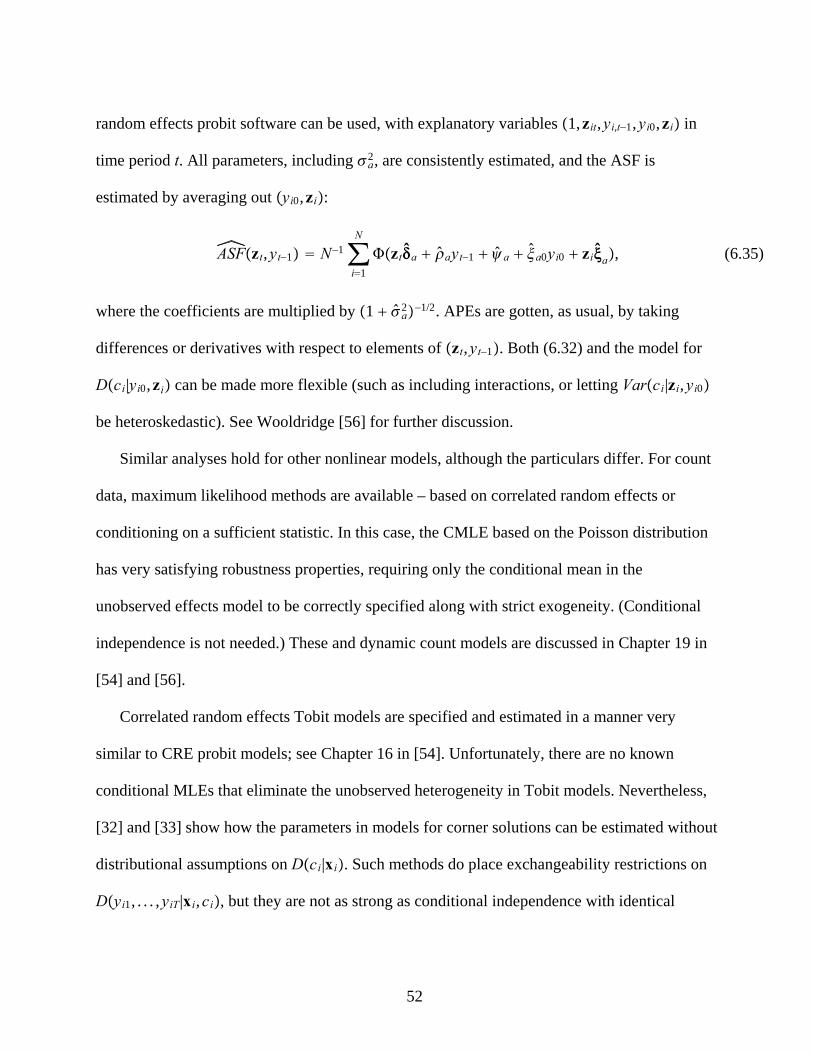
random effects probit software can be used, with explanatory variables 1,zit,yi,t−1,yi0,zi in

time period t. All parameters, including a2, are consistently estimated, and the ASF is

estimated by averaging out yi0,zi:

ASFzt,yt−1 N−1∑i1

N

zta ayt−1 a a0yi0 zia, (6.35)

where the coefficients are multiplied by 1 a2−1/2. APEs are gotten, as usual, by taking

differences or derivatives with respect to elements of zt,yt−1. Both (6.32) and the model for

Dci|yi0,zi can be made more flexible (such as including interactions, or letting Varci|zi,yi0

be heteroskedastic). See Wooldridge [56] for further discussion.

Similar analyses hold for other nonlinear models, although the particulars differ. For count

data, maximum likelihood methods are available – based on correlated random effects or

conditioning on a sufficient statistic. In this case, the CMLE based on the Poisson distribution

has very satisfying robustness properties, requiring only the conditional mean in the

unobserved effects model to be correctly specified along with strict exogeneity. (Conditional

independence is not needed.) These and dynamic count models are discussed in Chapter 19 in

[54] and [56].

Correlated random effects Tobit models are specified and estimated in a manner very

similar to CRE probit models; see Chapter 16 in [54]. Unfortunately, there are no known

conditional MLEs that eliminate the unobserved heterogeneity in Tobit models. Nevertheless,

[32] and [33] show how the parameters in models for corner solutions can be estimated without

distributional assumptions on Dci|xi. Such methods do place exchangeability restrictions on

Dyi1, . . . ,yiT|xi,ci, but they are not as strong as conditional independence with identical

52

distributions.

53

7. Other Topics and Future Directions

Research in panel data methods continues unabated. Dynamic linear models are a subject

of ongoing interest. The problem of feedback in linear models when the covariates are

persistent – and the weak instrument problem that it entails – is important for panels with small

T. For example, with firm-level panel data, the number of time periods is typically small and

inputs into a production function would often be well-approximated as random walks with

perhaps additional short-term dependence. The estimators described in Section 3.xx that

impose additional assumptions should be studied when those assumptions fail. Perhaps the

lower variance of the estimators from the misspecified model is worth the additional bias.

Models with random coefficients, especially when those random coefficients are on

non-strictly exogenous variables (such as lagged dependent variables), have received some

attention, but many of the proposed solutions require large T. (See, for example, [48] and [49].)

An alternative approach is flexible MLE, as in [56], where one models the distribution of

heterogeneity conditional on the initial condition and the history of covariates. See [57] for any

application to dynamic product choice.

When T is large enough so that it makes sense to use large-sample approximations with

large T, as well as large N, one must make explicit assumptions about the time series

dependence in the data. Such frameworks are sensible for modeling large geographical units,

such as states, provinces, or countries, where long stretches of time are observed. The same

estimators that are attractive for the fixed T case, particularly fixed effects, can have good

properties when T grows with N, but the properties depend on whether unit-specific effects,

time-specific effects, or both are included. The rates at which T and N are assumed to grow

also affect the large-sample approximations. See [51] for a survey of linear model methods

54

with T and N are both assumed to grow in the asymptotic analysis. A recent study that

considers estimation when the data have unit roots is [43]. Unlike the fixed T case, a unified

theory for linear models, let alone nonlinear models, remains elusive when T grows with N and

is an important area for future research.

In the models surveyed here, a single coefficient is assumed for the unobserved

heterogeneity, whereas the effect might change over time. In the linear model, the additive ci

can be replaced with tci (with 1 1 as a normalization). For example, the return to

unobserved managerial talent in a firm production function can change over time. Conditions

under which ignoring the time-varying loads, t, and using the usual fixed effects estimator,

consistently estimates the coefficients on xit are given in [46]. But one can also estimate the t

along with using method of moments frameworks. Examples are [31] and [1]. An area for

future research is to allow heterogeneous slopes on observed covariates along with

time-varying loads on the unobserved heterogeneity. Allowing for time-varying loads and

heterogeneous slopes in nonlinear models can allow for significant flexibility, but only

parametric approaches to estimation have been studied.

There is considerable interest in estimating production functions using proxy variables,

such as investment, for time-varying, unobserved productivity. The pioneering work is [47];

see also [41]. Estimation in this case does not rely on differencing or time-demeaning to

remove unobserved heterogeneity, and so the estimates can be considerably more precise than

the FE or FD estimators. But the assumption that a deterministic function of investment can

proxy for unobserved productivity is strong. [11] provides an analysis that explicitly allows for

unobserved heterogeneity and non-strictly exogenous inputs using the methods described in

Section 4. An interesting challenge for future researchers is to unify the two approaches to

55

exploit the attractive features of each.

The parametric correlated random effects approach for both static and dynamic nonlinear

models is now fairly well understood in the balanced case. Much less attention has been paid

to the unbalanced case, and missing data, especially for fully dynamic models, is a serious

challenge. [56] discusses the assumptions under which using a balanced subset produces

consistent estimates.

Identification of average partial effects (equivalently, the average structural function) has

recently received the attention that it deserves, although little is known about how robust are

the estimated APEs under various misspecifications of parametric models. One might hope that

using flexible models for nonlinear responses might provide good approximations, but

evidence on this issue is lacking.

As mentioned earlier, recent research in [3] has shown how to identify and estimate partial

effects without making parametric assumptions about Eyit|xit,c i or Dc i|xi. The setup in [3]

allows for Dc i|xi to depend on xi xi1, . . . ,xiT in an exchangeable way. The simplest case

is the one given in (6.15), Dc i|xi Dc i|xi. Under (6.15) and the strict exogeneity

assumption Eyit|xi,c i Eyit|xit,c i, the average structural function is identified as

ASFtxt E xirtxt, xi, (7.1)

where rtxit, xi Eyit|xit, xi. Because rtxit, xi can be estimated very generally – even

using nonparametric regression of yit on xit, xi for each t – the average partial effects can be

estimated without any parametric assumptions. Research in [3] shows how Dc i|xi can depend

on other exchangeable functions of xi1, . . . ,xiT, such as sample variances and covariances. As

discussed in [37], nonexchangeable functions, such as trends and growth rates, can be

accommodated, provided these functions are known. For example, for each i, let fi,ĝi be the

56

vectors of intercepts and slopes from the regression xit on 1, t, t 1, . . . ,T. Then, an extension

of (6.15) is Dci|xi Dci|fi,ĝi. It appears these kinds of assumptions have not yet been

applied, but they are a fertile area for future research because they extend the typical CRE

setup.

Future research on nonlinear models will likely consider the issue of the kinds of partial

effects that are of most interest. [3] studies identification and estimation of the local average

response (LAR). The LAR at xt for a continuous variable xtj is

∂mtxt,c∂xtjdHtc|xt, (7.2)

where mtxt,c is the conditional mean of the response and Htc|xt denotes the cdf of

Dc i|xit xt. This is a “local” partial effect because it averages out the heterogeneity for the

slice of the population described by the vector of observed covariates, xt. The APE averages

out over the entire distribution of c i, and therefore can be called a “global average response.”

See also [20]. The results in [3] include general identification results for the LAR, and future

empirical researchers using nonlinear panel data models may find the local nature of the LAR

more appealing (although more difficult to estimate) than APEs.

A different branch of the panel data literature has studied identification of coefficients or,

more often, scaled coefficients, in nonlinear models. For example, [34] shows how to estimate

in the model

yit 1wit xit ci uit ≥ 0 (7.3)

without distributional assumptions on the composite error, ci uit. In this model, wit is a

special continuous explanatory variable (which need not be time varying). Because its

coefficient is normalized to unity, wit necessarily affects the response, yit. More importantly,

57

wit is assumed to satisfy the distributional restriction Dci uit|wit,xit,zi Dci uit|xit,zi,

which is a conditional independence assumption. The vector zi is assumed to be independent

of uit in all time periods. (So, if two time periods are used, zi could be functions of variables

determined prior to the earliest time period.) The most likely scenario where the framework in

[34] applies is when wit is randomized and therefore independent of the entire vector

xit,zi,ci uit. The key condition seems unlikely to hold if wit is related to past outcomes on

yit. The estimator of derived in [34] is N -asymptotically normal, and fairly easy to

compute; it requires estimation of the density of wit given xit,ziand then a simple IV

estimation. Essentially by construction, estimation of partial effects on the response probability

is not possible.

Recently, [35] shows how to obtain bounds on parameters and APEs in dynamic models,

including the dynamic probit model in equation (6.29) under the strict exogeneity assumption

on zit : t 1, . . . ,T. A further assumption is that ci and zi are independent. By putting

restrictions on Dci – which nevertheless allow flexibility – [35] explains how to estimate

bounds for the unknown . The bounds allow one to determine how much information are in

the data when few assumptions are made. Similar calculations can be made for average partial

effects, so that the size of so-called state dependence – the difference between

Ecizt ci − zt ci – can be bounded.

Because CRE methods require some restriction on the distribution of heterogeneity, and

estimation of scaled coefficients leaves partial effects unidentified, the theoretical literature has

returned to the properties of parameter estimates and partial effects when the heterogeneity is

treated as unit-specific parameters to estimate. Recent work has focused on adjusting the

“fixed effects” estimates (of the common population parameters) so that they have reduced

58

bias.

An emerging question is whether the average partial effects might be estimated well even

though the parameters themselves are biased. In other words, suppose that for a nonlinear

model one obtains ,ĉ1,ĉ2, . . . ,ĉN, typically by maximizing a pooled log-likelihood function

across all i and t. If mtxt,c,, Eyt|xt,c is the conditional mean function, the average

partial effects can be estimated as

N−1∑i1

N∂mtxt,ĉ i,

∂xtj. (7.4)

In the unobserved effects probit model, (7.4) becomes

N−1∑i1

N

jxt ĉ i. (7.5)

[19] studied the properties of (7.5) with strictly exogenous regressors under conditional

independence, assuming that the covariates are weakly dependent over time. Interestingly, the

bias in (7.5) is of order T−2 when there is no heterogeneity, which suggests that estimating the

unobserved effects might not be especially harmful when the amount of heterogeneity is small.

Unfortunately, these findings do not carry over to models with time heterogeneity or lagged

dependent variables. While bias corrections are available, they are difficult to implement.

[23] proposes both jackknife and analytical bias corrections and show that they work well

for the probit case. Generally, the jackknife procedure to remove the bias in is simple but can

be computationally intensive. The idea is this. The estimator based on T time periods has

probability limit (as N → ) that can be written as

T b1/T b2/T2 OT−3 (7.6)

59

for vectors b1 and b2. Now, let t denote the estimator that drops time period t. Then,

assuming stability across t, it can be shown that the jackknife estimator,

T − T − 1T−1∑t1

T

t (7.7)

has asymptotic bias of on the order of T−2.

Unfortunately, there are currently some practical limitations to the jackknife procedure, as

well as to the analytical corrections derived in [23]. First, aggregate time effects are not

allowed, and they would be very difficult to include because the analysis is with T → . (In

other words, time effects would introduce an incidental parameters problem in the time

dimension, in addition to the incidental parameters problem in the cross section.) Plus,

heterogeneity in the distribution of the response yit across t changes the bias terms b1 and b2

when a time period is dropped, and so the adjustment in (7.7) does not remove the bias terms.

Second, [23] assumes independence across t conditional on ci. It is a traditional assumption,

but in static models it is often violated, and it must be violated in dynamic models. Plus, even

without time heterogeneity, the jackknife does not apply to dynamic models; see [22].

Another area that has seen a resurgence is so-called pseudo panel data, as initially

exposited in [18]. A pseudo-panel data set is constructed from repeated cross sections across

time, where the units appearing in each cross section are not repeated (or, if they are, it is a

coincidence and is ignored). If there is a natural grouping of the cross-sectional units – for

example, for individuals, birth year cohorts – one can create a pseudo-panel data set by

constructing group or cohort averages in each time period. With relatively few cohorts and

large cross sections, one can identify pseudo panels in the context of minimum distance

estimation. With a large number of groups, a different large-sample analysis might be

60

warranted. A recent contribution is [38] and [37] includes a recent survey. Open questions

include the most efficient way to use the full set of restrictions in the underlying

individual-level model.

As mentioned earlier, this chapter did not consider panel data model with explanatory

variables that are endogenous in the sense that they are correlated with time-varying

unobservables. For linear models, the usual fixed effects and first differencing transformations

can be combined with instrumental variables methods. In nonlinear models, the

Chamberlain-Mundlak approach can be combined with so-called “control function” methods,

provided the endogenous explanatory variables are continuous. [37] includes a discussion of

some recent advances for complicated models such as multinomial response models; see also

[50]. Generally, structural estimation in discrete response models with unobserved

heterogeneity and endogenous explanatory variables is an area of great interest.

61

Bibliography

Primary Literature

[1] Ahn, S.C. Y.H. Lee, and P. Schmidt (2001), “GMM Estimation of Linear Panel Data

Models with Time-Varying Individual Effects,” Journal of Econometrics 101, 219-255.

[2] Ahn, S.C. and P. Schmidt (1995), “Efficient Estimation of Models for Dynamic Panel

Data,” Journal of Econometrics 68, 5-27.

[3] Altonji, J.G. and R.L. Matzkin (2005), “Cross Section and Panel Data Estimators for

Nonseparable Models with Endogenous Regressors,” Econometrica 73, 1053-1102.

[4] Anderson, T.W. and C. Hsiao (1982), “Formulation and Estimation of Dynamic Models

Using Panel Data,” Journal of Econometrics 18, 47-82.

[5] Arellano, M. (1993), “On the Testing of Correlated Effects with Panel Data,” Journal of

Econometrics 59, 87-97.

[6] Arellano, M. and S.R. Bond (1991), “Some Tests of Specification for Panel Data:

Monte Carlo Evidence and an Application to Employment Equations,” Review of Economic

Studies 58, 277-297.

[7] Arellano, M. and O. Bover (1995), “Another Look at the Instrumental Variable

Estimation of Error Components Models,” Journal of Econometrics 68, 29-51.

[8] Arellano, M. and R. Carrasco (2003), “Binary Choice Panel Data Models with

Predetermined Variables,” Journal of Econometrics 115, 125-157.

[9] Arellano, M. and B. Honoré (2001), “Panel Data Models: Some Recent Developments,”

in Handbook of Econometrics, Volume 5, ed. J.J. Heckman and E. Leamer. Amsterdam: North

Holland, 3229-3296.

[10] Blundell, R. and S.R. Bond (1998), “Initial Conditions and Moment Restrictions in

62

Dynamic Panel Data Models,” Journal of Econometrics 87, 115-143.

[11] Blundell, R. and S.R. Bond (2000). “GMM Estimation with Persistent Panel Data: An

Application to Production Functions,” Econometric Reviews 19, 321-340.

[12] Blundell, R. and J.L. Powell (2003), “Endogeneity in Nonparametric and

Semiparametric Regression Models,” in Advances in Economics and Econonometrics: Theory

and Applications, Eighth World Congress, Volume 2, M. Dewatripont, L.P. Hansen and S.J.

Turnovsky, eds. Cambridge: Cambridge University Press, 312-357.

[13] Blundell, R. and R.J. Smith (1991), “Initial conditions and efficient estimation in

dynamic panel data models - an application to company investment behaviours,” Annales

d’économie et de statistique 20-21, 109-124.

[14] Cameron, A.C. and P.K. Trivedi (2005), Microeconometrics: Methods and

Applications. Cambridge: Cambridge University Press.

[15] Chamberlain, G. (1980), “Analysis of Covariance with Qualitative Data,” Review of

Economic Studies 47, 225-238.

[16] Chamberlain, G. (1982), “Multivariate Regression Models for Panel Data,” Journal of

Econometrics 1, 5-46.

[17] Chamberlain, G. (1984), “Panel Data,” in Handbook of Econometrics, Volume 2, ed.

Z. Griliches and M.D. Intriligator. Amsterdam: North Holland, 1248-1318.

[18] Deaton, A. (1985), “Panel Data from Time Series of Cross-Sections,” Journal of

Econometrics 30, 109-126.

[19] Fernández-Val, I. (2007), “Fixed Effects Estimation of Structural Parameters and

Marginal Effects in Panel Probit Models,” mimeo, Boston University Department of

Economics.

63

[20] Florens, J.P., J.J. Heckman, C. Meghir, and E. Vytlacil (2007), “Identification of

Treatment Effects Using Control Functions in Models with Continuous, Endogenous

Treatment and Heterogeneous Effects,” mimeo, Columbia University Department of

Economics.

[21] Hahn, J. (1999), “How Informative Is the Initial Condition in the Dynamic Panel

Model with Fixed Effects?” Journal of Econometrics 93, 309-326.

[22] Hahn, J. and G. Kuersteiner (2002), “Asymptotically Unbiased Inference for a

Dynamic Panel Model with Fixed Effects When Both n and T Are Large,” Econometrica 70,

1639-1657.

[23] Hahn, J. and W.K. Newey (2004), “Jackknife and Analytical Bias Reduction for

Nonlinear Panel Models,” Econometrica 72, 1295-1319.

[24] Hausman, J.A. (1978), “Specification Tests in Econometrics,” Econometrica 46,

1251-1271.

[25] Hausman, J.A. and W.E. Taylor (1981), “Panel Data and Unobservable Individual

Effects,” Econometrica 49, 1377-1398.

[26] Hayashi, F. (2000), Econometrics. Princeton, NJ: Princeton University Press.

[27] Heckman, J.J. (1976), “The Common Structure of Statistical Models of Truncation,

Sample Selection and Limited Dependent Variables and a Simple Estimator for Such Models,”

Annals of Economic and Social Measurement 5, 475-492.

[28] Heckman, J.J. (1981), “Statistical Models for Discrete Panel Data,” in Structural

Analysis of Discrete Data and Econometric Applications,” ed. C.F. Manski and D.L.

McFadden. Cambridge: MIT Press, 114-178.

[29] Heckman, J.J. (1981), “The Incidental Parameters Problem and the Problem of Initial

64

Condition in Estimating a Discrete Time-Discrete Data Stochastic Process,” in Structural

Analysis of Discrete Data and Econometric Applications, ed. C.F. Manski and D.L. McFadden.

Cambridge: MIT Press, 179-195..

[30] Hoch, I. (1962), “Estimation of production function parameters combining time-series

and cross-section data,” Econometrica 30 34-53.

[31] Holtz-Eakin, D., W. Newey, and H.S. Rosen (1988), “Estimating Vector

Autoregressions with Panel Data,” Econometrica 56, 1371-1395.

[32] Honoré, B.E. (1992), “Trimmed LAD and Least Squares Estimation of Truncated and

Censored Regression Models with Fixed Effects,” Econometrica 60, 533-565.

[33] Honoré, B.E. and L. Hu (2004), “Estimation of Cross Sectional and Panel Data

Censored Regression Models with Endogeneity,” Journal of Econometrics 122, 293-316.

[34] Honoré, B.E. and A. Lewbel (2002), “Semiparametric Binary Choice Panel Data

Models without Strictly Exogeneous Regressors,” Econometrica 70, 2053-2063.

[35] Honoré, B.E. and E. Tamer (2006), “Bounds on Parameters in Panel Dynamic Discrete

Choice Models,” Econometrica 74, 611-629.

[36] Im, K.S., S.C. Ahn, P. Schmidt, and J.M. Wooldridge (1999), “Efficient Estimation of

Panel Data Models with Strictly Exogenous Explanatory Variables” Journal of Econometrics

93, 177-201.

[37] Imbens, G.W. and J.M. Wooldridge (2007), “What’s New in Econometrics?” Lecture

Notes, National Bureau of Economic Research Summer Institute.

[38] Inoue, A. (2008), “Efficient Estimation and Inference in Linear Pseudo-Panel Data

Models,” Journal of Econometrics 142, 449-466.

[39] Keane, M.P. and D.E. Runkle (1992), “On the Estimation of Panel-Data Models with

65

Serial Correlation When Instruments Are Not Strictly Exogenous,” Journal of Business and

Economic Statistics 10, 1-9.

[40] Kiefer, N.M. (1980), “Estimation of Fixed Effect Models for Time Series of

Cross-Sections with Arbitrary Intertemporal Covariance,” Journal of Econometrics 14,

195-202.

[41] Levinshohn, J. and A. Petrin (2003), “Estimating Production Functions Using Inputs

to Control for Unobservables,” Review of Economic Studies 70, 317-341.

[42] Liang, K.-Y., and S.L. Zeger (1986), “Longitudinal Data Analysis Using Generalized

Linear Models,” Biometrika 73, 13-22.

[43] Moon, H.R. and P.C.B. Phillips (2004), “GMM Estimation of Autoregressive Roots

Near Unity with Panel Data,” Econometrica 72, 467-522.

[44] Mundlak, Y. (1961), “Empirical Production Function Free of Management Bias,” J.

Farm Econ.43, 44-56.

[45] Mundlak, Y. (1978), “On the Pooling of Time Series and Cross Section Data,

Econometrica 46, 69-85.

[46] Murtazashvili, I. and J.M. Wooldridge (2007), “Fixed Effects Instrumental Variables

Estimation in Correlated Random Coefficient Panel Data Models,” Journal of Econometrics

142, 539-552.

[47] Olley, S. and A. Pakes (1996), “The Dynamics of Productivity in the

Telecommunications Equipment Industry,” Econometrica 64, 1263-1298.

[48] Pesaran, M.H, R.P. Smith, and K.S. Im (1996), “Dynamic Linear Models for

Heterogeneous Panels,” in The Econometrics of Panel Data, ed. L. Mátáyas and P. Sevestre.

Dordrecht: Kluwer Academic Publishers, 145-195.

66

[49] Pesaran, M.H. and Y. Takashi (2008), “Testing Slope Homogeneity in Large Panels,”

Journal of Econometrics 142, 50-93.

[50] Petrin, A. and K.E. Train (2005), “Tests for Omitted Attributes in Differentiated

Product Models,” mimeo, University of Minnesota Department of Economics.

[51] Phillips, P.C.B. and H.R. Moon (2000), “Nonstationary Panel Data Analysis: An

Overview of Some Recent Developments,” Econometric Reviews 19, 263-286.

[52] Wooldridge, J.M. (1999), “Distribution-Free Estimation of Some Nonlinear Panel

Data Models,” Journal of Econometrics 90, 77-97.

[53] Wooldridge, J.M. (2000), “A Framework for Estimating Dynamic, Unobserved Effects

Panel Data Models with Possible Feedback to Future Explanatory Variables,” Economics

Letters 68, 245-250.

[54] Wooldridge, J.M. (2002), Econometric Analysis of Cross Section and Panel Data.

MIT Press: Cambridge, MA.

[55] Wooldridge, J.M. (2005), “Fixed-Effects and Related Estimators for Correlated

Random-Coefficient and Treatment-Effect Panel Data Models,” Review of Economics and

Statistics 87, 385-390.

[56] Wooldridge, J.M. (2005), “Simple Solutions to the Initial Conditions Problem in

Dynamic, Nonlinear Panel Data Models with Unobserved Heterogeneity,” Journal of Applied

Econometrics 20, 39-54.

[57] Erdem, T. and B. Sun (2001), “Testing for Choice Dynamics in Panel Data,” Journal

of Business and Economic Statistics 19, 142-152.

67

Books

Arellano, M. (2003), Panel Data Econometrics. Oxford: Oxford University Press.

Baltagi, B.H. (2001), Econometric Analysis of Panel Data, 2e. New York: Wiley.

Hsiao, C. (2003), Analysis of Panel Data, 2e. Cambridge: Cambridge University Press.

68