Embed Size (px)
Citation preview

Econometrics of Testing for Jumps inFinancial Economics Using BipowerVariation
Ole E. Barndorff-Nielsen
University of Aarhus
Neil Shephard
Nuffield College, University of Oxford
abstract
In this article we provide an asymptotic distribution theory for some nonpara-metric tests of the hypothesis that asset prices have continuous sample paths.We study the behaviour of the tests using simulated data and see that certainversions of the tests have good finite sample behavior. We also apply the tests toexchange rate data and show that the null of a continuous sample path isfrequently rejected. Most of the jumps the statistics identify are associated withgovernmental macroeconomic announcements.
keywords: bipower variation, jump process, quadratic variation, realizedvariance, semimartingales, stochastic volatility
In this article we will show how to use a time series of prices recorded at short
time intervals to estimate the contribution of jumps to the variation of asset prices
and form robust tests of the hypothesis that it is statistically satisfactory to regardthe data as if it has a continuous sample path. Being able to distinguish between
jumps and continuous sample path price movements is important as it has
implications for risk management and asset allocation. A stream of recent articles
in financial econometrics has addressed this issue using low-frequency return
data based on (i) the parametric models of Andersen, Benzoni, and Lund (2002),
Chernov et al. (2003), and Eraker, Johannes, and Polson (2003); (ii) the Markovian,
doi:10.1093/jjfinec/nbi022
Advance Access publication August 19, 2005
ª The Author 2005. Published by Oxford University Press. All rights reserved. For permissions,
please e-mail: [email protected].
Ole Barndorff-Nielsen’s work is supported by CAF, funded by the Danish Social Science Research Council. Neil
Shephard’s research is supported by the U.K.’s ESRC. The Ox language of Doornik (2001) was used to perform
the calculations reported here. We have benefited from comments from Tim Bollerslev, Clive Bowsher, Xin
Huang, Jean Jacod, Jeremy Large, Bent Nielsen, and three anonymous referees on an earlier draft of this article.
Address correspondence to Ole E. Barndorff-Nielsen, Department of Mathematical Sciences, University of
Aarhus, Ny Munkegade, DK-8000 Aarhus C, Denmark, or E-mail: [email protected].
Journal of Financial Econometrics, 2006, Vol. 4, No. 1, 1–30
at Duke U
niversity on January 17, 2014http://jfec.oxfordjournals.org/
Dow
nloaded from

nonparametric analysis of Aıt-Sahalia (2002), Bandi and Nguyen (2003), and
Johannes (2004); (iii) options data [e.g., Bates (1996) and the review by Garcia,
Ghysels, and Renault (2005)]. Our approach will be nonparametric and exploit
high-frequency data. Monte Carlo results suggest that it performs well whenbased on empirically relevant sample sizes. Furthermore, empirical work points
us to the conclusion that jumps are common.
Traditionally, in the theory of financial economics, the variation of asset prices is
measured by looking at sums of squared returns calculated over small time periods.
The mathematics of that is based on the quadratic variation process [e.g., Back (1991)].
Asset pricing theory links the dynamics of increments of quadratic variation to the
increments of the risk premium. The recent econometric work on this topic, estimating
quadratic variation using discrete returns under the general heading of realized quad-ratic variation, realized volatility, and realized variances, was discussed in independent
and concurrent work by Andersen and Bollerslev (1998), Comte and Renault (1998), and
Barndorff-Nielsen and Shephard (2001). It was later developed in the context of the
methodology of forecasting by Andersen et al. (2001), while central limit theorems for
realized variances were developed by Jacod (1994), Barndorff-Nielsen and Shephard
(2002), and Mykland and Zhang (2005). Multivariate generalizations to realized covaria-
tion are discussed by, for example, Barndorff-Nielsen and Shephard (2004a) and Ander-
sen et al. (2003a). See Andersen, Bollerslev, and Diebold (2005) and Barndorff-Nielsenand Shephard (2005) for surveys of this area and references to related work.
Recently Barndorff-Nielsen and Shephard (2004b) introduced a partial gen-
eralization of quadratic variation called bipower variation (BPV). They showed
that in some cases relevant to financial economics, BPV can be used, in theory, to
split up the individual components of quadratic variation into that due to the
continuous part of prices and that due to jumps. In turn, the bipower variation
process can be consistently estimated using an equally spaced discretization of
financial data. This estimator is called the realized bipower variation process.In this article we study the difference or ratio of realized BPV and realized
quadratic variation. We show we can use these statistics to construct nonparametric
tests for the presence of jumps. We derive the asymptotic distributional theory for
these tests under quite weak conditions. This is the main contribution of this article. We
will also illustrate the jump tests using both simulations and exchange rate data. We
relate some of the jumps to macroeconomic announcements by government agencies.
A by-product of our research is an appendix that records a proof of the con-
sistency of realized BPV under substantially weaker conditions than those used byBarndorff-Nielsen and Shephard (2004b). The appendix also gives the first derivation
of the joint limiting distribution for realized BPV and the corresponding realized
quadratic variation process under the assumption that there are no jumps in the price
process. The latter result demonstrates the expected conclusion that realized BPV is
slightly less efficient than the realized quadratic variation as an estimator of quad-
ratic variation in the case where prices have a continuous sample path.
Since we wrote the first draft of this article, we have teamed up with the
probabilists Svend Erik Graversen, Jean Jacod, and Mark Podolskij to relax theseconditions further. In particular, we report in Barndorff-Nielsen et al. (2005) some
2 Journal of Financial Econometrics
at Duke U
niversity on January 17, 2014http://jfec.oxfordjournals.org/
Dow
nloaded from

results on generalized BPV that largely removes the regularity assumptions used
in this article. To do this we use very advanced probabilistic ideas that make the
results rather inaccessible. Hence we think it is still valuable to publish the original
results, which can be proved using relatively elementary methods. We willaugment these results with comments that show how far Barndorff-Nielsen et al.
(2005) were able to go in removing the assumptions we use in this article.
In the next section we will set out our notation and recall the definitions of quadratic
variation and BPV. In Section 2 we give the main theorem of the article, which is the
asymptotic distribution of the proposed tests. In Section 3 we will extend the analysis to
cover the case of a time series of daily statistics for testing for jumps. In Section 4 we study
how the jump tests behave in simulation studies, while in Section 5 we apply the theory to
two exchange rate series. In Section 6 we discuss various additional issues, while Section 7concludes. The proofs of the main results in the article are given in the appendix.
1 DEFINITIONS AND PREVIOUS WORK
1.1 Notation and Quadratic Variation
Let the log-price of a single asset be written as Yt for continuous time t � 0. Y is
assumed to be a semimartingale. For a discussion of economic aspects of this see
Back (1991). Further, Yd will denote the purely discontinuous component of Y,while Yc will be the continuous part of the local martingale component of Y.
The quadratic variation (QV) process of Y can be defined as
½Y�t ¼ p� limn!1
Xn�1
j¼0
ðYtjþ1� Ytj
Þ2, ð1Þ
[e.g., Jacod and Shiryaev (1987:55)] for any sequence of partitions t0 = 0 < t1
< . . . < tn = t with supj{tj+1 – tj} ! 0 for n!1. It is well known that
½Y�t ¼ ½Yc�t þ ½Yd�t, where ½Yd�t ¼X
0�u�t
DY2u, ð2Þ
and DYt ¼ Yt � Yt� are the jumps in Y. We will test for jumps by asking if [Y] = [Yc].
We estimated [Y] using a discretized version of Y based on intervals of timeof length d > 0. The resulting process, which we write as Yd, is Yd[t/d], for t � 0,
recalling that [x] is the integer part of x. This allows us to construct �-returns
yj ¼ Yjd � Yðj�1Þd, j ¼ 1, 2,:::, ½t=d�,
which are used in the realized quadratic variation process,
½Yd�t ¼X½t=d�j¼1
y2j ,
the QV of Y�. Clearly the QV theory means that as d # 0; ½Yd�t!p ½Y�t.
Our analysis of jumps will often be based on the special case where Y is a
member of the Brownian semimartingale plus jump (BSMJ) class:
Barndorff-Nielsen & Shephard | Econometrics of Testing for Jumps 3
at Duke U
niversity on January 17, 2014http://jfec.oxfordjournals.org/
Dow
nloaded from

Yt ¼Z t
0
asdsþZ t
0
ssdWs þ Zt, ð3Þ
where Z is a jump process. In this article we assume that
Zt ¼XNt
j¼1
cj,
with N being a simple counting process (which is assumed finite for all t) and the
cj are nonzero random variables. Further we assume a is cadlag, the volatility � is
cadlag, and W is a standard Brownian motion. When N � 0, we write Y 2 BSM,
which is a stochastic volatility plus drift model [e.g., Ghysels, Harvey, and
Renault (1996)]. In this case, ½Yc�t ¼R t
0 s2s ds and ½Yd�t ¼
PNt
j¼1 c2j , so
½Y�t ¼Z t
0
s2s dsþ
XNt
j¼1
c2j :
1.2 Bipower Variation
The 1, 1-order BPV process is defined, when it exists, as
fYg½1,1�t ¼ p� lim
d#0
X½t=d�j¼2
jyj�1jjyjj: ð4Þ
Barndorff-Nielsen and Shephard (2004b) showed that if Y2BSMJ, a � 0 and � isindependent from W then
fYg½1,1�t ¼ m2
1
Z t
0
s2sds ¼ m2
1½Yc�t,
where
m1 ¼ Ejuj ¼ffiffiffi2p
=ffiffiffipp
^ 0:79788 ð5Þ
and u˜ N(0, 1). Hence m�21 fYg
½1;1� ¼ ½Yc�. This result is quite robust, as it does not
depend on any other assumptions concerning the structure of N, the distribution of
the jumps, or the relationship between the jump process and the SV component. The
reason for this is that only a finite number of terms in Equation (4) are affected by
jumps, while each return that does not have a jump goes to zero in probability.
Therefore, since the probability of jumps in contiguous time intervals goes to zero asd # 0, those terms do not impact the probability limit.
Clearly {Yg½1;1�t can be consistently estimated by the realized BPV process
fYdg½1,1�t ¼
X½t=d�j¼2
jyj�1jjyjj,
4 Journal of Financial Econometrics
at Duke U
niversity on January 17, 2014http://jfec.oxfordjournals.org/
Dow
nloaded from
as d # 0. One would expect these results on BPV to continue to hold when we
extend the analysis to allow a 6¼ 0. This is indeed the case, as will be discussed in
the next section.
Barndorff-Nielsen and Shephard (2004b) point out that
½Y�t � m�21 fYg
½1;1�t ¼
XNt
j¼1
c2j ¼ ½Yd�t:
This can be consistently estimated by ½Yd�t � m�21 fYdg½1;1�t . Hence, in theory, the
realized BPV process can be used to consistently estimate the continuous and
discontinuous components of QV or, if augmented with the appropriate asymp-
totic distribution theory, as a basis for testing the hypothesis that prices have
continuous sample paths.
The only other work we know which tries to split QV into that due to thecontinuous and the jump components is Mancini (2004). She does this via the
introduction of a jump threshold whose absolute value goes to zero as the number
of observations within each day goes to infinity. Related work includes Coutin
(1994). Following Barndorff-Nielsen and Shephard (2004b), Woerner (2004a) stu-
died the robustness of realized power variation d1�r=2P½t=d�j¼1 jyjjr to an infinite
number of jumps in finite time periods showing that the robustness property of
realized power variation goes through in that case. A related article is Aıt-Sahalia
(2004), which shows that maximum-likelihood estimation can disentangle ahomoskedastic diffusive component from a purely discontinuous infinite activity
Levy component of prices. Outside the likelihood framework, the article also
studies the optimal combinations of moment functions for the generalized
method of moments estimation of homoskedastic jump diffusions.
2 A THEORY FOR TESTING FOR JUMPS
2.1 Infeasible Tests
In this section we give the main contribution of the article, Theorem 1. It gives the
asymptotic distribution for a linear jump statistic, G, based on m�21 fYdg½1;1�t � ½Yd�t
and a ratio jump statistic, H, based on1m�21 fYdg½1;1�t =½Yd�t. Their distributions, under
the null of Y 2 BSM, will be seen to depend upon the unknown integrated
quarticityR t
0 s4udu, and so we will say the results of the theorem are statistically
infeasible. We will overcome this problem in the next subsection.
Recall the definition m1 ¼ffiffiffi2p
=ffiffiffipp
in Equation (5) and let
W ¼ ðp2=4Þ þ p� 5^ 0:6090: ð6Þ
1 Following Barndorff-Nielsen and Shephard (2004b), Huang and Tauchen (2005) have independently and
concurrently used simulations to study the behavior of this type of ratio, although they do not provide the
corresponding asymptotic theory.
Barndorff-Nielsen & Shephard | Econometrics of Testing for Jumps 5
at Duke U
niversity on January 17, 2014http://jfec.oxfordjournals.org/
Dow
nloaded from

Theorem 1 Let Y2 BSM and let t be a fixed, arbitrary time. Suppose the following
conditions are satisfied:
(a) The volatility process �2 is pathwise bounded away from zero.
(b) The joint process (a, �) is independent of the Brownian motion W.
Then as �#0
G ¼d�1=2 m�2
1 fYdg½1,1�t � ½Yd�t
� �ffiffiffiffiffiffiffiffiffiffiffiffiffiffiffiffiffiffiffiR t
0 Ws4udu
q !L Nð0,1Þ, ð7Þ
and
H ¼d�1=2 m�2
1 fYdg½1,1�t
½Yd�t� 1
� �ffiffiffiffiffiffiffiffiffiffiffiffiffiffiffiffiffiffiffiffiffiffiffiWR t
0s4
s dsR t
0s2
s ds
n o2
vuut!L Nð0,1Þ: ð8Þ
Further, if Y 2 BSMJ and (a) and (b) hold, then
fYg½1,1�t ¼ m2
1
Z t
0
s2s ds: ð9Þ
Remark 1
(i) Condition (a) in Theorem 1 holds, for instance, for the square-root process
(due to it having a reflecting barrier at zero) and the Ornstein-Uhlenbeck
volatility processes considered in Barndorff-Nielsen and Shephard (2001).
More generally (a) does not rule out jumps, diurnal effect, long memory, or
breaks in the volatility process.
(ii) It is clear from the proof of Theorem 1 that in realized BPV we can replace
the subscript j – 1 with j – q, where q is any positive but finite integer.
(iii) Condition (b) rules out leverage effect [e.g., Black (1976), Nelson (1991),
and Ghysels, Harvey, and Renault (1996)] and feedback between previous
innovations in W and the risk premium in at. This is an unfortunate
important limitation of the result. This is often regarded to be empirically
reasonable with exchange rules, but clashes with what we observe for equity
data [e.g., Hansen and Lunde (2005)]. Simulation results in Huang and
Tauchen (2005) suggest the behavior of the test statistic is not affected by
leverage effects. The results in Barndorff-Nielsen et al. (2005) confirm this.
6 Journal of Financial Econometrics
at Duke U
niversity on January 17, 2014http://jfec.oxfordjournals.org/
Dow
nloaded from

They show the central limit theorem of Equation (7) holds if at is a locally
bounded, predictable process and �2 follows, for example,
s2t ¼ s2
0 þZ t
0
a0sdWs þZ t
0
v0s�dLs,
where a0 and v0 are locally bounded, predictable processes and L is a Levy
process (which can include a Brownian component) independent of W. The
�2 process thus includes all diffusive models for volatility, but also allows for
some types of jumps. This structure is relaxed in their paper even further to
allow for more general forms of jumps, but the resulting conditions are
highly technical and so we will not discuss them here.
(iv) Equation (9) means that under the alternative hypothesis of jumps
m�21 fYdg½1,1�
t � ½Yd�t!p�XNt
j¼1
c2j � 0
and
m�21 fYdg½1,1�
t
½Yd�t� 1!
p�
PNt
j¼1 c2jRt
0
s2s dsþ
PNt
j¼1 c2j
� 0:
This implies the linear and ratio tests will be consistent.
(v) A by-product of the proof of Theorem 1 is Theorem 3, given in the appendix,
which is a joint central limit theorem for scaled realized BPV and QV
processes. This is proved under the assumption that Y 2 BSM and shows
that they, of course, both estimateR t
0 �2s ds, with the efficient realized QV
having a slightly smaller asymptotic variance. Thus we can think of
Equation (7) as a Hausman (1978)-type test, a point first made by
Huang and Tauchen (2005) following the initial draft of this article.
2.2 Feasible Tests
To construct computable linear and ratio jump tests we need to estimate
the integrated quarticityR t
0 s4udu under the null hypothesis of Y2 BSM. However,
in order to ensure the test has power under the alternative, it is preferable to
have an estimator of integrated quarticity that is also consistent under the
alternative BSMJ. This is straightforward using realized quadpower variation,
fYdg½1;1;1;1�t ¼ d�1X½t=d�j¼4
jyj�3jjyj�2jjyj�1jjyjj!pm4
1
Z t
0
s4s ds:
The validity of this result when there are no jumps is discussed in Barndorff-Nielsen
et al. (2005). The robustness to jumps is straightforward so long as there are a finite
number of jumps. It also holds in cases where the jump component Z of the BSMJ model
is a Levy or non-Gaussian OU model [see Barndorff-Nielsen, Shephard, and Winkel(2004)].
Barndorff-Nielsen & Shephard | Econometrics of Testing for Jumps 7
at Duke U
niversity on January 17, 2014http://jfec.oxfordjournals.org/
Dow
nloaded from

The above discussion allows us to define the feasible linear jump test statistic,
G, which has the asymptotic distribution
G ¼d�1=2 m�2
t fYdg½1,1�t � ½Yd�t
� �ffiffiffiffiffiffiffiffiffiffiffiffiffiffiffiffiffiffiffiffiffiffiffiffiffiffiffiffiffiffiffiffiWm�4
1 fYdg½1,1,1,1�t
q !L Nð0,1Þ, ð10Þ
where we would reject the null of a continuous sample path if Equation
(10) is significantly negative. Likewise, the ratio jump test statistic, H, defined
as
H ¼ d�1=2ffiffiffiffiffiffiffiffiffiffiffiffiffiffiffiffiffiffiffiffiffiffiffiffiffiffiffiffiffiffiffiffiffiffiffiffiffiffiffiffiffiffiffiffiffiffiffiffiffiffiffiWfYdg½1,1,1,1�
t = fYdg½1,1�t
n o2r m�2
1 fYdg½1,1�t
½Yd�t� 1
!!L Nð0,1Þ, ð11Þ
rejects the null if significantly negative.
The ratio fYdg½1;1�t =½Yd�t is asymptotically equivalent to the realized corre-
lation between |yj-1| and |yj| [e.g., Barndorff-Nielsen and Shephard (2004a)].
It converges to m12^0.6366 under BSM. Estimates below m2
1 provide evidence
for jumps. Its asymptotic distribution under the null follows trivially from
Equation (11). Further, in Equation (8), clearly the ratio
Rt0
s4s ds=
Rt0
s2s ds
!2
� 1=t, with equality obtained in the homoskedastic case. This
suggests replacing H by the adjusted ratio jump test
J ¼ d�1=2ffiffiffiffiffiffiffiffiffiffiffiffiffiffiffiffiffiffiffiffiffiffiffiffiffiffiffiffiffiffiffiffiffiffiffiffiffiffiffiffiffiffiffiffiffiffiffiffiffiffiffiffiffiffiffiffiffiffiffiffiffiffiffiffiffiffiffiffiffiffiffiffiffiffiffiWmax t�1,fYdg½1,1,1,1�
t = fYdg½1,1�t
n o2� �s m�2
1 fYdg½1,1�t
½Yd�t� 1
!!L Nð0,1Þ:
3 TIME SERIES OF REALIZED QUANTITIES
To ease the exposition we will use t = 1 to denote the period of a day. Then we
define
vi ¼X½1=d�j¼1
Ydjþði�1Þ � Ydðj�1Þþði�1Þ� �2 ¼ ½Yd�i � ½Yd�ði�1Þ; i ¼ 1; 2; :::;T;
the daily increments of realized QV, so as d # 0 then vi!p ½Y�i � ½Y�ði�1Þ. The vi
andffiffiffiffivi
pare called the daily realized variance and volatility in financial
economics, respectively. Here we give the corresponding results for realized
BPV and then discuss the asymptotic theory for a time series of such
sequences. These results follow straightforwardly from our previous theore-
tical results.
8 Journal of Financial Econometrics
at Duke U
niversity on January 17, 2014http://jfec.oxfordjournals.org/
Dow
nloaded from

Clearly we can define a sequence of T daily realized BPVs,
vi ¼X½1=d�j¼2
jyj�1;ijjyj;ij; i ¼ 1; 2; :::;T;
where we assume � satisfies d½1=d� ¼ 1 for ease of exposition and
yj;i ¼ Ydjþði�1Þ � Ydðj�1þði�1Þ:
Clearly m�21 vi!p ½Yc�i � ½Yc�ði�1Þ. In order to develop a feasible limit theory it
will be convenient to introduce a sequence of daily realized quadpower
variations,
qi ¼ d�1X½1=d�j¼4
jyj�3;ijjyj�2;ijjyj�1;ijjyj;ij; i ¼ 1; 2; :::;T:
The above sequence of realized quantities suggest constructing a sequence of
nonoverlapping, feasible daily jump test statistics:
Gdi ¼d�1=2 m�2
1 vi � vi
� �ffiffiffiffiffiffiffiffiffiffiffiffiffiffiWm�4
1 qi
q , ð12Þ
Hdi ¼d�1=2 m�2
1 vi
vi� 1
� �ffiffiffiffiffiffiffiffiffiffiffiffiffiffiffiffiffiffiffiWfqi=vig2
q , ð13Þ
Jdi ¼d�1=2ffiffiffiffiffiffiffiffiffiffiffiffiffiffiffiffiffiffiffiffiffiffiffiffiffiffiffiffiffiffiffiffiffiffiffiffiffiffi
Wmax 1,qi=fvig2
� �r ��21 vi
vi� 1
� �: ð14Þ
By inspecting the proof of Theorem 1, it is clear that as well as each of theseindividual tests converging to N (0, 1) as d # 0, the converge as a sequence in time
jointly to a multivariate normal distribution. For example, define a sequence of
feasible ratio tests Hd ¼ ðHd1;:::;HdTÞ0, then as d # 0 so Hd!L Nð0; ITÞ. Likewise
Gd!L Nð0; ITÞand Jd!L Nð0; ITÞ. Thus each of these tests have the property that
they are asymptotically serially independent through time, under the null
hypothesis that there are no jumps.
4 SIMULATION STUDY
4.1 Simulation Design
In this section we document some Monte Carlo experiments that assess the
finite sample performance of our asymptotic theory for the feasible tests for
jumps. Throughout, we assume Y 2 BSMJ, but set a � 0 and the component
processes �, W, N, and c to be independent. Before we start we should
Barndorff-Nielsen & Shephard | Econometrics of Testing for Jumps 9
at Duke U
niversity on January 17, 2014http://jfec.oxfordjournals.org/
Dow
nloaded from

mention that in independent and concurrent work Huang and Tauchen (2005)
also studied the finite sample behavior of our central limit theory using an
extensive simulation experiment. Their conclusions are broadly in line with
the ones we reach here.2
Our model for � is derived from some empirical work reported in
Barndorff-Nielsen and Shephard (2002), who used realized variances to fit
the spot variance of the deutsch mark (DM) dollar rate from 1986 to 1996 by
the sum of two uncorrelated, stationary processes, s2 ¼ s21 þ s2
2. Their results
are compatible with using Cox, Ingersoll and Ross (CIR) processes for the
s21 and s2
2 processes. In particular, we will write these, for s = 1, 2, as the
solution to
ds2t,s ¼ �ls s2
t,s � xs
dtþ osst,s dBlst,s, xs � o2
s=2, ð15Þ
where B = (B1, B2)0 is a vector standard Brownian motion, independent from W.
Equation (15) has a gamma marginal distribution,
s2t;s � Ga 2o�2
s xs; 2o�2s
� �¼ Gaðns; asÞ; ns � 1;
with a mean of ns=as and a variance of ns=a2s [Cox, Ingersoll, and Ross (1985)]. The
parameters !s, �s, and �s were calibrated by Barndorff-Nielsen and Shepard (2002)as follows. Setting p1 + p2 = 1, they estimated
Eðs2s Þ ¼ ps0:509; varðs2
s Þ ¼ ps0:461; s ¼ 1; 2;
with p1 = 0.218, p2 = 0.782, �1 = 0.0429, and �2 = 3.74, which means the first,
smaller component of the variance process is slowly reverting with a half-life of
about 16 days, while the second has a half-life of about 4 hours.All jumps will be generated by taking N as K jumps uniformly scattered
in each unit of time. We call this a stratified Poisson process, using the
terminology of sample survey theory, [e.g., Kish (1965)]. This setup means
that when K > 0, we can view the power of the test conditionally as the
probability of rejection in time units where there actually were jumps. We
specify cj �i:i:d:Nð0; s2c Þ, so the variance of Yd
t and Yct are tKs2
c and t0.509, respec-
tively. We will vary K and s2c , which allows us to see the impact of the
frequency of jumps and their size on the behavior of the realized bipowervariation process. To start off, we will fix K = 2 and s2
c ¼ 0:2� 0:509, which
means that the jump process will account for 28% of the variation of the
process. Clearly this is a high proportion. Later we will study the cases when
K = 1 and s2c ¼ 0:1� 0:509 and 0.05 � 0.509.
Finally, the results will be indexed by n = 1/d, the number of observations per
unit of time.
2 Huang and Tauchen (2005) also report results on the finite sample behavior of the test when it is carried
out over long stretches of data, such as 1 year or 10 years. In this case, the results differ from the ones
given here with significant size distortions. As Huang and Tauchen (2005) explain, this is not surprising,
and this effect is also present when we look at the behavior of the asymptotic theory for realized quadratic
variation. See also the work of Corradi and Distaso (2004).
10 Journal of Financial Econometrics
at Duke U
niversity on January 17, 2014http://jfec.oxfordjournals.org/
Dow
nloaded from

4.2 Null Distribution
We will use 5000 simulated days to assess the finite sample behavior of the jumptests given in Equations (12), (13), and (14). We start by looking at their null
distributions when N � 0.
The left-hand side of Figure 1 shows the results from the first 300 days in the
sample. The crosses depict the linear difference m�21 vi � vi, while the feasible 99%
one-sided critical values [using Equation (12)] of the difference are given by the solid
line. As we go down the graph, n increases, and so, as the null hypothesis is true, the
magnitude of m�21 vi � vi and corresponding critical values tend to fall toward zero.
The most important aspect of these graphs is that the critical values of the testschange dramatically through time, reflecting the volatility clustering in the data.
The second column of Figure 1 repeats this analysis, but now using the jump
ratio m�21 vi=vi � 1, which tends to fall as n increases. The feasible critical values of
this ratio are more stable through time, reflecting the natural scale invariance of
the denominator for the ratio jump tests. The third column shows the results for
the adjusted critical values. This has some differences from the unadjusted ver-
sion when n is small. The right-hand side of Figure 1 shows the QQ plots of the
t-tests of Equations (12), (13), and (14). On the y-axis are the ranked values of thesimulated t-tests, while on the x-axis are the corresponding expected values under
Gaussian sampling. We see a very poor QQ plot for the linear test, even when
Figure 1 Simulation from the null distribution of the feasible limit theory for the linear differencem�2
1 vi � vi and jump ratios m�21 vi=vi � 1
� �for a variety of values of n. Also given are the corre-
sponding results for the adjusted version. Also shown is the 99% one –sided critical value of thestatistics. Right-hand side gives the QQ plots of the three sets of t-statistics.
Barndorff-Nielsen & Shephard | Econometrics of Testing for Jumps 11
at Duke U
niversity on January 17, 2014http://jfec.oxfordjournals.org/
Dow
nloaded from

n = 72. For larger values of n, the asymptotics seem to have some substantial bite.
The ratio test has quite good QQ plots for n � 72.
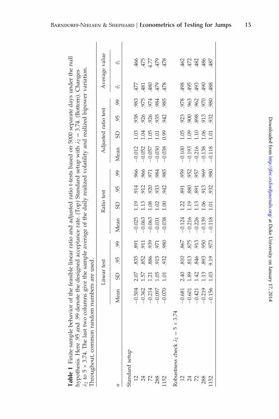
In the upper part of Table 1 we show the means, standard deviations and
acceptance rates (defined as the probability of not rejecting the null hypothesis) ofEquations (12), (13), and (14). Under the asymptotics, they should ideally have values,
0, 1, .95, and .99, respectively. All three statistics have a negative mean, leading to
overrejection of the null due to the one-sided nature of the test. Even when n = 288,
the linear test rejects the null around 8%, rather than 5%, of the time. The small
sample performance of the adjusted ratio test is better for a range of values of n.
As a final check on the null distribution of the jump tests, we repeat the above
analysis, but increasing �2, the mean reversion parameter of the fast decaying
volatility process, by a factor of five. This reduces its half-life down to 20 minutes.This case of an extremely short half-life is quite a challenge, as a number of
econometricians view very short memory SV models as being good proxies for
processes with jumps. Table 1 shows the results. The linear test has a negative bias
that reduces as n becomes very large. The ratio test has a smaller negative bias and
overreject less than the linear test. The degree of overrejection is modest, but more
important than in the first simulation design. Hence this testing procedure can be
challenged by very fast reverting volatility components.
4.3 Impact of Jumps: The Alternative Distribution
We now introduce some jumps into the process and see how the tests react. The
stratified Poisson process is set up to have either one or two jumps per day, while
the variance of the jumps is either 5%, 10%, or 20% of Eðs2t Þ.
The results are given in Table 2 and they are in line with expectations. There
is little difference in the nominal power of the linear and adjusted ratio tests. As
the number of jumps or the variance of the jumps increases, so the rate of
accepting the null falls. In the case where there is a single jump per day and the
jump is 5% of the variability of the continuous component of prices, we reject the
null 20% of the time when n = 288.
One of the interesting features of Table 2 is that the probability of accepting the
null is roughly similar if N = 2 and each jump is 10% of the variation of �2
compared to the case where N = 1 and we look at the 20% example. This is repeated
when we move to the N = 2 and 5% case and compare it to the N = 1 and 10% case.
This suggests the rejection rate is heavily influenced by the variance of the jump
process, not just the frequency of the jumps or the size of the individual jumps.
5 TESTING FOR JUMPS EMPIRICALLY
5.1 Dataset
We now turn our attention to using the adjusted ratio jump test of Equation (14)
on economic data. We use the bivariate German DM/U.S. dollar and Japanese
yen/U.S. dollar exchange rate series, which covers the 10-year period from
December 1, 1986, until November 30, 1996. Hence if the dollar generally
12 Journal of Financial Econometrics
at Duke U
niversity on January 17, 2014http://jfec.oxfordjournals.org/
Dow
nloaded from
Ta
ble
1F
init
esa
mp
leb
ehav
ior
of
the
feas
ible
lin
ear
rati
oan
dad
just
edra
tio
t-te
sts
bas
edo
n50
00se
par
ate
day
su
nd
erth
en
ull
hy
po
thes
is.
Her
e.9
5an
d.9
9d
eno
teth
ed
esig
ned
acce
pta
nce
rate
.(T
op
)S
tan
dar
dse
tup
wit
hl 2¼
3:74:
(Bo
tto
m).
Ch
ang
esl 2
to5�
3:74
.T
he
last
two
colu
mn
sg
ive
the
sam
ple
aver
age
of
the
dai
lyre
aliz
edv
ola
tili
tyan
dre
aliz
edb
ipo
wer
var
iati
on
.T
hro
ug
ho
ut,
com
mo
nra
nd
om
nu
mb
ers
are
use
d.
Lin
ear
test
Rat
iote
stA
dju
sted
rati
ote
stA
ver
age
val
ue
nM
ean
SD
.95
.99
Mea
nS
D.9
5.9
9M
ean
SD
.95
.99
vi
v i
Sta
nd
ard
setu
p
12�
0.50
42.
07.8
35.8
91�
0.02
51.
19.9
14.9
66�
0.01
21.
03.9
38.9
83.4
77.4
66
24�
0.36
21.
57.8
52.9
11�
0.06
31.
13.9
12.9
66�
0.05
21.
04.9
26.9
75.4
81.4
75
72�
0.21
41.
21.8
86.9
39�
0.06
31.
08.9
20.9
71�
0.05
71.
05.9
26.9
74.4
804.
77
288
�0.
097
1.05
.915
.971
�0.
031
1.02
.933
.984
�0.
030
1.01
.935
.984
.479
.479
1152
�0.
070
1.01
.932
.980
�0.
038
1.00
.942
.985
�0.
038
0.99
.942
.985
.478
.478
Ro
bu
stn
ess
chec
kl 2¼
5�
3:74
12�
0.68
12.
40.8
10.8
67�
0.12
41.
22.8
91.9
59�
0.10
01.
05.9
23.9
78.4
98.4
62
24�
0.60
11.
89.8
13.8
75�
0.21
61.
19.8
80.9
52�
0.19
31.
09.9
00.9
63.4
95.4
72
72�
0.42
11.
42.8
46.9
13�
0.22
61.
13.8
91.9
57�
0.21
61.
10.8
98.9
62.4
93.4
82
288
�0.
219
1.13
.893
.950
�0.
139
1.06
.913
.969
�0.
138
1.06
.913
.970
.490
.486
1152
�0.
156
1.03
9.19
.973
�0.
118
1.01
.932
.980
�0.
118
1.01
.932
.980
.488
.487
Barndorff-Nielsen & Shephard | Econometrics of Testing for Jumps 13
at Duke U
niversity on January 17, 2014http://jfec.oxfordjournals.org/
Dow
nloaded from

strengthens, both of these rates would be expected to rise. The original dataset
records every five minutes the most recent midquote to appear on the Reuters
screen. We have multiplied all returns by 100 in order to make them easier to
present. The database has been kindly supplied to us by Olsen and Associates,Zurich, Switzerland, who document their ground breaking work in this area in
Dacorogna et al. (2001).
5.2 Ratio Jump Statistic
Figure 2 plots the ratio statistic m�21 vi=vi and its corresponding 99% critical values,
computed under the assumption of no jump using the adjusted theory given in
Equation (14), for each of the first 250 working days in the sample for n = 12 and
n = 72. We reject the null if the ratio is significantly less than one. The values of n
are quite small, corresponding to 2-hour and 20-minute returns, respectively.
Results for larger values of n will be reported in a moment. Of importance is
that the critical values do not change very much between different days.
Figure 2 shows quite a lot of rejections of the null of no jumps, although thetimes where the rejections are statistically significant sometimes change with n.
When n is small, the rejections are marginal (note the Monte Carlo results suggest
one should not trust the decisions based on the test with such small samples
unless the test is absolutely overwhelming, which is not the case here), but by the
0 50 100 150 200 250
0.5
1.0
1.5 n=12. Dollar/DMRatio statisticCritical value
0 50 100 150 200 250
0.25
0.50
0.75
1.00
1.25
Dollar/Yen
0 50 100 150 200 250
0.50
0.75
1.00
1.25n=72.
Days 0 50 100 150 200 250
0.25
0.50
0.75
1.00
1.25
Days
Figure 2 Based on the first year of the sample for the dollar/DM (left-hand side) and dollar/yen(right-hand side) using n = 12 and n = 72. Index plot shows the ratio statistic m�2
1 vi=vi computedeach day, which should be about one if the null of no jumps is true. The corresponding 99%adjusted asymptotic critical value is also shown.
14 Journal of Financial Econometrics
at Duke U
niversity on January 17, 2014http://jfec.oxfordjournals.org/
Dow
nloaded from

Ta
ble
2E
ffec
to
fju
mp
so
nth
eli
nea
ran
dad
just
edra
tio
test
s.O
nth
eri
gh
t-h
and
sid
ew
esh
ow
resu
lts
for
the
case
wh
ere
ther
ear
etw
oju
mp
sp
erd
ay.O
nth
ele
fth
and
sid
e,th
ere
isa
sin
gle
jum
pp
erd
ay.T
he
var
ian
ces
of
the
jum
ps
are
20%
,10%
,an
d5%
,res
pec
tiv
ely
,of
the
exp
ecta
tio
no
fs2
,w
ith
the
resu
lts
for
the
20%
case
giv
enat
the
top
.T
he
last
two
colu
mn
sg
ive
the
sam
ple
aver
age
of
the
dai
lyre
aliz
edv
ola
tili
tyan
dre
aliz
edb
ipo
wer
var
iati
on
.T
hro
ug
ho
ut,
com
mo
nra
nd
om
nu
mb
ers
are
use
d.
Lin
ear
test
Rat
iote
stA
dju
sted
rati
on
test
Av
erag
ev
alu
e
Mea
nS
D.9
5.9
9M
ean
SD
.95
.99
Mea
nS
D.9
5.9
9v i
vi
20%
,N1=
2
12�
0.78
2.33
.787
.851
�0.
181.
25.8
81.9
53�
0.15
1.08
.911
.975
.578
.545
24�
0.94
2.28
.756
.827
�0.
411.
28.8
31.9
17�
0.37
1.18
.853
.937
.584
.542
72�
1.64
2.92
.653
.740
�0.
991.
60.7
10.8
12�
0.96
1.55
.720
.819
.584
.527
288
�3.
845.
56.4
32.5
32�
2.51
2.76
.464
.573
�2.
502.
75.4
65.5
74.5
82.5
08
1152
�8.
8211
.6.2
47.3
09�
5.80
5.44
.255
.325
�5.
805.
44.2
55.3
25.5
81.4
94
10%
,N1=
2
12�
0.58
2.03
.813
.878
�0.
081.
20.9
02.9
64�
0.07
1.04
.929
.983
.527
.510
24�
0.58
1.80
.816
.877
�0.
211.
19.8
81.9
51�
0.18
1.09
.899
.965
.532
.514
72�
0.80
1.81
.774
.849
�0.
501.
30.8
18.9
04�
0.48
1.26
.825
.913
.532
.508
288
�1.
802.
94.6
18.7
18�
1.35
1.95
.651
.761
�1.
341.
94.6
52.7
62.5
31.4
98
1152
�4.
245.
89.4
00.4
84�
3.28
3.69
.412
.503
�3.
283.
69.4
13.5
03.5
30.4
88
5%,N
1=
2
12�
0.52
1.97
.829
.886
�0.
041.
18.9
10.9
67�
0.03
1.02
.937
.984
.502
.489
24�
0.43
1.63
.838
.900
�0.
111.
15.9
02.9
64�
0.09
1.06
.918
.974
.507
.497
72�
0.43
1.38
.840
.907
�0.
241.
14.8
85.9
54�
0.23
1.11
.892
.961
.506
.496
288
�0.
831.
73.7
66.8
57�
0.66
1.41
.795
.888
�0.
661.
40.7
95.8
89.5
05.4
91
1152
�2.
003.
06.5
79.6
86�
1.71
2.36
.596
.707
�1.
712.
36.5
96.7
07.5
04.4
85
con
tin
ued
Barndorff-Nielsen & Shephard | Econometrics of Testing for Jumps 15
at Duke U
niversity on January 17, 2014http://jfec.oxfordjournals.org/
Dow
nloaded from

Ta
ble
2(c
onti
nu
ed)
Lin
ear
test
Rat
iote
stA
dju
sted
rati
ote
stA
ver
age
val
ue
Mea
nS
D.9
5.9
9M
ean
SD
.95
.99
Mea
nS
D.9
5.9
9v
iv i
20%
,N1=
1
12�
0.9
32.
65.7
69.8
34�
0.23
1.29
.862
.937
�0.
191.
12.8
96.9
64.5
79.5
34
24�
1.13
2.90
.732
.808
�0.
471.
35.8
13.9
03�
0.43
1.24
.837
.921
.584
.531
72�
1.90
3.72
.644
.726
�1.
061.
76.6
96.7
91�
1.03
1.71
.706
.766
.583
.515
288
�4.
217.
40.4
95.5
73�
2.48
3.18
.520
.608
�2.
473.
17.5
20.6
09.5
83.5
00
1152
�9.
2915
.5.3
55.4
19�
5.51
6.32
.364
.432
�5.
516.
32.3
64.4
32.5
82.4
89
10%
,N1=
1
12�
0.65
2.24
.807
.864
�0.
111.
22.8
93.9
56�
0.09
1.06
.924
.978
.527
.505
24�
0.66
2.01
.799
.867
�0.
241.
22.8
69.9
40�
0.22
1.13
.886
.954
.532
.509
72�
0.95
2.13
.752
.827
�0.
581.
40.7
98.8
91�
0.56
1.35
.804
897
.531
.502
288
�2.
033.
83.6
30.7
16�
1.42
2.26
.659
.748
�1.
412.
25.6
60.7
49.5
31.4
93
5%,N
1=
1
12�
0.55
2.14
.824
.882
�0.
051.
19.9
07.9
64�
0.03
1.04
.932
.982
.502
.488
24�
0.46
1.69
.832
.894
�0.
131.
16.8
97.9
57�
0.11
1.07
.912
.970
.507
.495
72�
0.51
1.49
.823
.896
�0.
301.
19.8
68.9
45�
0.28
1.15
.875
.951
.506
.492
288
�0.
972.
12.7
49.8
36�
0.74
1.59
.776
.868
�0.
741.
58.7
78.8
70.5
05.4
88
1152
�2.
193.
96.6
07.7
06�
1.78
2.81
.623
.723
�1.
782.
81.6
23.7
23.5
04.4
83
16 Journal of Financial Econometrics
at Duke U
niversity on January 17, 2014http://jfec.oxfordjournals.org/
Dow
nloaded from

time n = 72, there is strong evidence for the presence of some specific jumps. In
both cases and for both series, the average ratio is less than one. When n = 12, the
percentage of ratios less than one is 70% and 73%, while when n increases to 72
these percentages become 71% in both cases.Table 3 reports the corresponding results for the whole 10-year sample. This
table, which provides a warning of the use of too high a value of n, shows the
sum, denoted r., of the first to fifth serial correlation coefficients of the high-
frequency data. We see that in the DM/dollar series, as n increases, this correla-
tion builds up, probably due to bid/ask bounce effects. By the time n has
reached 288, the summed correlation has reached nearly -0.1, which means the
realized variance overestimates the variability of prices by around 20%. Of
course, this effect could be removed by using a further level of prefilteringbefore we analyse the data. The situation is worse for the yen/dollar series,
which has a moderate amount of negative correlation among the high-frequency
returns even when n is quite small. We will ignore these market microstructure
effects here.
Table 3 shows the average value of m�21 vi and vi as well as the proportion of
times the null is rejected using 95% and 99% asymptotic tests. These values are
given for a variety of values of n and for both exchange rates. The results are
reasonably stable with respect to n, although the percentage due to jumps doesdrift as n changes.
The table shows that for the DM/dollar series, the variation of the jumps is
estimated to contribute between about 5% and 20% of the QV. On 20% of days, the
hypothesis of no jumps is rejected at the 5% asymptotic level, while at the 1%
asymptotic level, this falls to 10%. The results for the yen/dollar are rather
similar. These results should be viewed tentatively, as the Monte Carlo results
suggest there are finite sample biases in the critical values, even when we ignore
market microstructure effects. However, the statistical evidence does push ustoward believing there are jumps in the price processes. Interestingly, the percen-
tage of rejections and proportions due to jumps seem rather stable as we move
between the two exchange rates.
5.3 Case Studies
To illustrate this methodology we will apply the jump test to the DM/dollar rate,
asking if the hypothesis of a continuous sample path is consistent with the data
we have. To start, we will give a detailed discussion of an extreme day—Friday,
January 15, 1988—which we will put in context by analyzing it together with a
few days before the extreme event. In Figure 3 we plot 100 times the discretized
Y�, so a one-unit uptick represents a 1% change, for a variety of values of n = 1/d,
as well as giving the ratio jump statistics m�21 vi=vi with their corresponding 99%
critical values.
In Figure 3 there is a large uptick in the DM against the dollar, with a
movement of nearly 2% in a five-minute period. This occurred on Friday and
was a response to the news of a large decrease in the U.S. balance of payment
Barndorff-Nielsen & Shephard | Econometrics of Testing for Jumps 17
at Duke U
niversity on January 17, 2014http://jfec.oxfordjournals.org/
Dow
nloaded from

deficit, which lead to a large strengthening of the dollar. The Financial Times
reported on its front page the next day:
The dollar and share prices soared in hectic trading on world financial
markets yesterday after the release of official figures showing that the US
Table 3 r. denotes the sum of the first five serial correlation coefficients of thehigh-frequency data. BPV denotes the average value of m�2
1 vi over the sample.QV gives the corresponding result for vi. Jump % is the percentage of the quadraticvariation due to jumps in the sample. 5% rej. and 1% rej. show the proportion ofrejections at the 5% and 1% levels, respectively.
Dollar/DM Dollar/yen
N r. BPV QV Jump % 5% rej. 1% rej. r. BPV QV Jump % 5% rej. 1% rej.
12 .001 .355 .452 21.5 .202 .090 �.041 .328 .420 21.9 .201 .086
48 .012 .408 .467 12.6 .219 .114 �.032 .409 .458 10.7 .209 .101
72 �.001 .437 .487 10.2 .225 .120 �.032 .429 .471 8.9 .195 .095
144 �.056 .471 .510 7.6 .220 .116 �.077 .473 .506 6.5 .223 .107
288 �.092 .502 .531 5.4 .181 .092 �.100 .512 .539 5.0 .187 .095
0
1
2
3
4 Change in Yδ during week using δ=20 minutes
Mon FriThursWedTues
0.50
0.75
1.00
Ratio jump statistic and 99% critical values
Mon Tues Wed Thurs Fri
(μ1)−2~vi/vi99% critical values
0
1
2
3
4 Change in Yδ during week using δ=5 minutes
Mon Tues Wed Thurs Fri0.25
0.50
0.75
1.00
Ratio jump statistic and 99% critical values
Mon Tues Wed Thurs Fri
(μ1)−2~vi/vi99% critical values
Figure 3 (Left) Discretized sample paths of the exchange rate, centered at zero on Monday, January 11,1988, and running until Friday of that week. Drawn every 20 and 5 minutes. An up-tick of one indicatesstrengthening of the dollar by 1%. (Right) shows an index plot, starting at one, of m�2
1 vi=vi, whichshould be about one if there are no jumps. Test is one sided, with critical values also drawn as a line.
18 Journal of Financial Econometrics
at Duke U
niversity on January 17, 2014http://jfec.oxfordjournals.org/
Dow
nloaded from
trade deficit had fallen to $13.22 bn in November from October’s record
level of $17.63 bn. The US currency surged 4 pfennigs and 4 yen within 10
minutes of the release of the figures and maintained the day’s highest
levels in late New York business. . ..’’
The data for Friday had a large realized variance, but a much smaller
estimate of the integrated variance. Hence the statistics are attributing a large
component of the realized variance to the jump, with the adjusted ratio statistic
being larger than the corresponding 99% critical value. When � is large, thestatistic is on the borderline of being significant, while the situation becomes
much clearer as � becomes small.
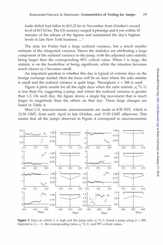
An important question is whether this day is typical of extreme days on the
foreign exchange market. Here the focus will be on days where the ratio statistic
is small and the realized variance is quite large. Throughout n = 288 is used.
Figure 4 plots results for all the eight days when the ratio statistic m�21 vi=vi
is less than 0.6, suggesting a jump, and where the realized variance is greater
than 1.2. On each day, the figure shows a single big movement that is muchlarger in magnitude than the others on that day. These large changes are
listed in Table 4.
Most U.S. macroeconomic announcements are made at 8:30 EST, which is
12:30 GMT, from early April to late October, and 13:30 GMT otherwise. This
means that all the jumps observed in Figure 4 correspond to macroeconomic
171 172 173
–0.5
0.0
0.5
171 172 173
0.50
0.75
1.00
232 233 234
–2
–1
0
232 233 234
0.50
0.75
1.00
251 252 253
0
2
4
251 252 253
0.50
0.75
1.00
271 272 273
0
1
2
271 272 273
0.6
0.8
1.0
310 311 312
–1
0
310 311 312
0.50
0.75
1.00
331 332 333
0.0
0.5
1.0
331 332 333
0.50
0.75
1.00
414 415 416
0
1
2
Days414 415 416
0.50
0.75
1.00
Days681 682 683
0.0
0.5
1.0
1.5
Days681 682 683
0.6
0.8
1.0
Days
Figure 4 Days on which vi is high and the jump ratio m�21 vi=vi found a jump using n = 288.
Depicted is Yd � Yi; the corresponding ratios m�21 vi=vi, and 99% critical values.
Barndorff-Nielsen & Shephard | Econometrics of Testing for Jumps 19
at Duke U
niversity on January 17, 2014http://jfec.oxfordjournals.org/
Dow
nloaded from

announcements. There is substantial economic literature trying to relate move-
ments in exchange rates to macroeconomic announcements [e.g., Ederington and
Lee (1993) and Andersen, Bollerslev, Diebold, and Vega (2003b)]. Generally this
concludes that such news is quickly absorbed into the market, moving the rates
vigourously, but with little long-term impact on the subsequent volatility of the
rates, which is very much in line with what we saw in Figure 3.
6 CONCLUSION
In this article we provide a test to ask, for a given time series of prices
recorded every � time periods, if it is statistically satisfactory to regard the
data as if it had a continuous sample path. We derive the asymptotic dis-
tribution of the testing procedure as � # 0 under the null of no jumps and
ignoring the possible impact of market microstructure effects. Monte Carlo
results suggest an adjusted ratio jump statistic can be reliably used to test for
jumps if � is moderately small and the test is carried out over relatively short
periods, such as a day. We applied this test to some exchange rate data andfound many rejections of the null of no jumps. In some case studies we
related the rejections to macroeconomic news.
The article opens up a number of technical questions. Can multivariate
versions of these ideas be developed so one can detect common jumps across
assets? How robust is bipower variation to market microstructure effects and can
these effects be moderated in some way? We are currently researching on these
topics with various coauthors and hope to report results on them soon. Another
question is whether bipower variation is robust to infinite activity jump pro-cesses—that is, jump processes with an infinite number of jumps in a finite time
interval? This is a technically demanding question and is addressed in recent work
by Woerner (2004b) and Barndorff-Nielsen, Shephard, and Winkel (2004).
The article also naturally points to a number of economic issues. Can specific
types of economic news be formally linked to the jumps indicated by these tests?
Can the tests for jumps be used to improve volatility forecasts? Research on the
second of these points has been recently reported by Andersen, Bollerslev, and
Diebold (2003) and Forsberg and Ghysels (2004).
Table 4 Days and times at which there seems significant evidence that therehas been a jump.
Sequence Day GMT Move
173th Friday, September 11, 1987 12.35 �.967
234th Thursday, December 10, 1987 13.35 �1.44
253th Friday, January 15, 1988 13.35 2.03
273th Friday, February 12, 1988 13.35 1.16
312th Thursday, April 14, 1988 12.35 �1.65
333th Tuesday, May 17, 1988 12.35 1.14
416th Wednesday, September 14, 1988 12.35 0.955
20 Journal of Financial Econometrics
at Duke U
niversity on January 17, 2014http://jfec.oxfordjournals.org/
Dow
nloaded from

APPENDIX A: PROOF OF THEOREM 1
A.1 Assumptions and Statement of Two Theorems
In this appendix we prove two results we state in this subsection: (i) Theorem 2,
which shows consistency of realized BPV; (ii) Theorem 3, which gives a joint
central limit theory for realized BPV and QV under BSM. These two results then
deliver Theorem 1 immediately. Sometimes we will refer to the unnormalizedversion of the r, s order of realized BPV,
Yd½ �½r,s�t ¼
Xn
j¼2
jyj�1jrjyjjs, r,s > 0:
Clearly
Yd½ �½1,1�t ¼ fYdg½1,1�
t ,
which is of central interest.
We will derive the limit results for a fixed value of t, and without loss of
generality we assume that [t/�] is integer, writing t = �n. So as � # 0, then necessarily
n!1. The general approach in our proofs is to study the limit theory condition-
ally on (a, �). The unconditional limit results then follow trivially, as, in the present
circumstances, conditional convergence implies global convergence.Recall the two assumptions we use in Theorem 1.
(a) The volatility process � is pathwise bounded away from zero.
(b) The joint process (a, �) is independent of the Brownian motion W.
Note also that our general precondition that � is cadlag implies that � is
pathwise bounded away from 1.
Theorem 2 Let Y 2 BSMJ and suppose conditions (a) and (b) hold, then
fYg½1,1�t ¼ m2
1
Z t
0
s2s ds: ð16Þ
Theorem 3 Let Y 2 BSM and suppose conditions (a) and (b) hold. Then conditionally
on (a, �), the realized QV and BPV processes
½Yd�t and m�21 fYdg½1,1�
t ð17Þ
follow asymptotically, as � # 0, a bivariate normal law with common meanR t
0 �2s ds: The
asymptotic covariance of
d�1=2 ½Yd�tm�2
1 fYdg½1,1�t
!�
R t0 s
2s dsR t
0 s2s ds
! #"
Barndorff-Nielsen & Shephard | Econometrics of Testing for Jumps 21
at Duke U
niversity on January 17, 2014http://jfec.oxfordjournals.org/
Dow
nloaded from

is
PZ t
0
s4s ds ð18Þ
where
P ¼ varðu2Þ2m�2
1Covðu2;jujju0 jÞ
2m�21 Covðu2;jujju0 jÞ
m�41fvarðjujju0 jÞþ2covðjujju0 j;ju0 jju0 0 jÞg
� �
¼ 22
2ðp2=4Þþp�3
� �^ 2
222:6090
� �with u, u’, u’’ being independent standard normals.
A.2 Consistency of Realized BPV: Theorem 2
Once the theorem is proved in the no jumps case, the general result follows trivially
using the argument given in Barndorff-Nielsen and Shephard (2004b). Here we there-
fore assume Y 2 BSM. The proof goes in three stages. We provide some preliminary
results on discretization of integrated variance. Then we recall the consistency of BPV
when a = 0, and finally we show that allowing a 6¼ 0 has negligible impact.For the latter conclusion we only need to establish that the impact of a is of
order op(1). However, for the proof of Theorem 3 we require order opð�1=2Þ: That
this holds is verified separately in the next subsection.
We first recall a result, which is obtained in the course of the proof of
Theorem 2 of Barndorff-Nielsen and Shephard [2004b, cf. Equation (13)].
Proposition 1 [Barndorff-Nielsen and Shephard (2004b)] Under (a) we have for any
r>0 and �2j ¼
R j�
ðj�1Þ� �2s ds that
d1�rXn
j¼2
srj�1s
rj �Xn
j¼1
s2rj
8<:
9=; ¼ OpðdÞ:
Corollary 1 Under (a) we have that
Xn
j¼2
sj�1sj �Z t
0
s2s ds ¼ OpðdÞ:
This corollary is a special case of the previous proposition and follows from
the fact thatPn
j¼1 s2j ¼
R t0 s
2s ds.
The following is a restatement of Theorem 2 in Barndorff-Nielsen and
Shephard (2004b) in the case where r = s = 1. It will be used to prove Theorem 3.
22 Journal of Financial Econometrics
at Duke U
niversity on January 17, 2014http://jfec.oxfordjournals.org/
Dow
nloaded from

Theorem 4 Suppose Y 2 BSM and in addition (a), (b), and a = 0, then
Xn
j¼2
jyj�1jjyjj
0@
1A� m2
1
Z t
0
s2s ds ¼ opð1Þ:
To complete the proof of Theorem 2 we need to show that the impact of the
drift is negligible. As already mentioned, this follows from the stronger result,
Proposition 2 which we derive in the next subsection.
A.3 Negligibility of Drift
For simplicity of notation we now write Mt ¼R t
0 ssdWs, which, conditional on s,
has a Gaussian law with a zero mean and variance ofR t
0 s2sds. To establish that the
effect of the drift is negligible in the contexts of Theorems 2 and 3 it suffices toshow that, under conditions (a) and (b),
½Yd�½1,1�t � ½Md�½1,1�
t ¼ opðd1=2Þ:
In fact, we shall prove the following stronger result, which covers a variety ofversions of realized BPV. To do this we will use the notation
hrðu;rÞ ¼ jrd1=2 þ ujr � jujr,
hr,sðu,v;r1,r2Þ ¼ jr1d1=2 þ ujrjr2d
1=2 þ vjs � jujrjvjs:
For reasons of compactness we often write hr;sðu; v;r1; r2Þ as hr;sðu; v;rÞ, wherer ¼ ðr1; r2Þ
0.
Proposition 2 Under conditions (a) and (b), for any r; s > 0 and for every
e 2 0; 14
� �½Yd�½r,s� � ½Md�½r,s� ¼ Opðdðrþs�1Þ=2þeÞ:
Proof. Let s2 ¼ inf0�s�ts2s and s2 ¼ sup0�s�ts
2s ;mj ¼Mjd �M j�1ð Þd and
s2j ¼
R dj
dðj�1Þ s2s ds,
gj ¼ d�1aj, aj ¼Z dj
dðj�1Þasds, j ¼ 1,2,:::, n:
Note that (pathwise for ða; sÞ), by assumption (a), 0 < s2 � s2 < 1, implying
if yjd ¼ s2j ; then 0 < minj yj � maxj yj<1, while, due to a being cadlag,
there exists (pathwise) a constant c for which maxjjgjj � c, whatever the value
of n.
Barndorff-Nielsen & Shephard | Econometrics of Testing for Jumps 23
at Duke U
niversity on January 17, 2014http://jfec.oxfordjournals.org/
Dow
nloaded from

We have, using (b) and writing now mjL sjjujj, where the uj �
i:i:d:Nð0; 1Þ,that
½Yd�½r,s�t � ½Md�½r,s�
t ¼Pnj¼2
ðjaj�1 þmj�1jsjaj þmjjr � jmj�1jsjmjjrÞ
¼Pnj¼2
fjdgj�1 þ d1=2y1=2j�1uj�1jsjdgj þ d1=2y1=2
j ujjr
�jd1=2y1=2j�1uj�1jsjd1=2y1=2
j ujjrg
¼ dr=2ds=2Pnj¼2
ys=2j�1y
r=2j fjðgj�1=y
1=2j�1Þd
1=2
þuj�1js jðgj=y1=2j Þd
1=2 þ ujjr � juj�1jsjujjrg
and hence
d�ðrþsÞ=2 ½Yd�½r,s�t � ½Md�½r,s�
t
n o¼Xn
j¼2
ys=2j�1y
r=2j hr,s uj�1,uj;gj�1=y
1=2j�1,gj=y
1=2j
� �:
As jgj=y1=2j j is bounded for all j, the conclusion of Proposition 2 now follows
from Corollary 2, below. &
To obtain that corollary, we establish three lemmas—1, 2, and 3. Lemma 1
collates several results from Barndorff-Nielsen and Shephard (2003) which are
used to prove Lemmas 2 and 3.
Lemma 1 [Barndorff-Nielsen and Shephard (2003)] For any r > 0 and � � 0, we
have
Efhrðu;rÞg ¼ OðdÞ, Efjujrhrðu;rÞg ¼ Oðdð1þ16rÞ=2Þ,
Efh2r ðu;rÞg ¼ Oðdð1þ16rÞ=2Þ, varfhrðu;rÞg ¼ Oðdð1þ16r=2Þ:
The results given in Lemma 1 are derived in the course of the proof of
Proposition 3.3 in Barndorff-Nielsen and Shephard (2003), so a separate proof
will not be given here.We proceed to state and prove Lemmas 2 and 3.
Lemma 2 For any r; s > 0; u; v�i:i:d:Nð0; 1Þ and �1 and �2 nonnegative constants, we have
Efhr,sðu,v;r1,r2Þ ¼ OðdÞ:
Proof. The independence of u, v together with the first equation in Lemma 1
implies
24 Journal of Financial Econometrics
at Duke U
niversity on January 17, 2014http://jfec.oxfordjournals.org/
Dow
nloaded from

Efhr,s,ðu,v;rÞg ¼ E jr1d1=2 þ ujr
n oE jr2d
1=2 þ ujsn o
� EfjujrgEfjvjsg
¼ Efhrðu;r1ÞgEfhsðv;r2Þg þ Efhrðu;r1ÞgEfjvjsg
þEfhsðv;r2ÞgEfjujrg ¼ OðdÞ: &
Lemma 3 For u, v independent standard normal random variables and �1 and �2
nonnegative constants, we have
Efh2r,sðu,v;r1,r2Þg ¼ O dð1þ16r6sÞ=2
� �:
Proof. Clearly
h2r,sðu,v;rÞ ¼ jr1d
1=2 þ uj2rjr2d1=2 þ vj2s þ juj2rjvj2s � 2jr1d
1=2 þ ujrjr2d1=2 þ vjsjujrjvjs
¼ h2r,2sðu,v;rÞ þ 2juj2rjvj2s � 2jr1d1=2 þ ujrjr2d
1=2 þ vjsjujrjvjs,
so, by Lemma 2 and the independence of u and v,
Efh2r,sðu,v;rÞg ¼ Efh2r,2sðu,v;rÞg þ 2Efjuj2rgEfjuj2sg
�2E jujrjr1d1=2 þ ujr
n oE jujsjr2d
1=2 þ ujsn o
¼ OðdÞ � 2 E jujrjr1d1=2 þ ujr
n oE jujsjr2d
1=2 þ ujsn o�
�Efjuj2rgEjuj2sgÞ:
Furthermore,
E jujrjr1d1=2 þ ujr
n oE jujsjr2d
1=2 þ ujsn o
� E juj2rn o
E juj2sn o
¼ E jujrjr1d1=2 þ ujr � juj2r
n oE jujsjr2d
1=2 þ ujsn o
þE juj2rn o
E jujsjr2d1=2 þ ujs
n o� E juj2r
n oE juj2sn o
¼ E jujrjr1d1=2 þ ujr � juj2r
n oE jujsjr2d
1=2 þ ujs � juj2sn o
þE juj2sn o
E jujrjr1d1=2 þ ujr � juj2r
n o
þE juj2rn o
E jujsjr2d1=2 þ ujs
n o� E juj2r
n oE juj2sn o
¼ E jujrhr u;r1ð Þf gE jujshs u;r2ð Þf g
þE juj2sn o
E jujrhr u;r1ð Þf g þ E juj2rn o
E jujshs u;r2ð Þf g:All in all, on account of Lemma 1, this means that
Barndorff-Nielsen & Shephard | Econometrics of Testing for Jumps 25
at Duke U
niversity on January 17, 2014http://jfec.oxfordjournals.org/
Dow
nloaded from

E h2r,s u,v;r1,r2ð Þ
¼ O dð Þ þO d 1þ16rð Þ=2
� �O d 1þ16sð Þ=2� �
þO d 1þ16rð Þ=2� �
þO d 1þ16sð Þ=2� �
¼ O d 1þ16r6sð Þ=2� �
: &
Lemmas 2 and 3 and the Cauchy-Schwarz inequality together imply
Corollary 2 For u, v, v0independent standard normal random variables and �1, �2, �01, �02
nonnegative constants, we have
var hr,s u,v;r1,r2ð Þf g ¼ O d 1þ16r6sð Þ=2� �
and
cov hr,s u,v;r1,r2ð Þ,hr,s u,v0;r01,r02� �
¼ O d 1þ16r6sð Þ=2� �
:
As already mentioned, the conclusion of Proposition 2 follows from Corollary 2.
Remark 2 From the final equation in the proof of Lemma 3, one sees that in the special
case when r = s = 1, then
var h1,1 u,v;r1,r2ð Þf g ¼ O dð Þ,
and hence the conclusion of Proposition 2 may be sharpened to [Y�][1,1] – [M�]
[1,1] =
Op(�).
A.4 Asymptotic Distribution of BPV: Theorem 3
Given Proposition 2, what remains is to prove Theorem 3 when Y2BSM and
the additional conditions (a), (b), and a = 0 hold. The key feature is that,
ignoring the asymptotically negligible y21 and conditioning on the � process,
we have that
Pnj¼2 y2
jPnj¼2 jyj�1jjyjj
!�
R t0 s
2s ds
m21
R t0 s
2s ds
0@
1A
is asymptotically equivalent in law to
Xn
j¼2
s2j vj
sj�1sjwj
!
26 Journal of Financial Econometrics
at Duke U
niversity on January 17, 2014http://jfec.oxfordjournals.org/
Dow
nloaded from
where vj ¼ u2j � 1;wj ¼ juj�1jjujj � m2
1, and uj �i:i:dN 0; 1ð Þ. The sequences {vj} and {wj}
have zero means, with the former being i.i.d., while the latter satisfy wj wj+s for
|s|>1. Then the theorem follows if we can show that
d�1=2Xn
j¼2
s2j vj
sj�1sjwj
!!L N 0,
Z t
0
s4s ds
var v1ð Þ 2cov v1,w1ð Þ2cov v1,w1ð Þ var w1ð Þ þ 2cov w1,w2ð Þ
� �� �:
ð19Þ
Our strategy for proving this is to show3 the limiting Gaussian result using anyreal constants c1 and c2,
d�1=2Xn
j¼2
c1s2j vj þ c2sj�1sjwj
� �
!L N 0,
Z t
0
s4s ds c2
1Var v1ð Þ þ 4c1c2cov v1,w1ð Þ þ c22 var w1ð Þ þ 2cov w1,w2ð Þf g
� �� �:
The asymptotic Gaussianity follows from standard calculations from the classical
central limit theorem for martingale sequences due to Lipster and Shiryaev [e.g.,
Shiryayev (1981: 216)].
What remains is to derive the asymptotic variance of this sum. Let use
define
cj ¼
ffiffiffiffiffiffiffiffiffiffiffiffiffiffiffiffiffiffiffiffiffiffiffiffiffiffiffiffiffiffiffiffid�1
Z dj
d j�1ð Þs2
s ds:
s
Clearly
d�1=2Xn
j¼2
c1s2j vj þ c2sj�1sjwj
� �¼ d1=2
Xn
j¼2
c1c2j vj þ c2cj�1cjwj
� �
has the variance
dXn
j¼2
var c1c2j vj þ c2cj�1cjwj
� �þ 2d
Xn
j¼3
cov c2cj�1cjwj, c2cj�2cj�1wj�1
� �
þ 2dXn
j¼2
cov c1c2j�1vj�1,c2cj�1cjwj
� �:
3 Recall that if zn = (zn1, ... znq) is a sequence of random vectors having mean zero, then to prove that zn!L Nq
(0, �) for some nonnegative definite matrix �, it suffices to show that for arbitrary real constants c1,...,cq
we have c0zn!L Nqð0, c0� c), where c = (c1, ..., cq)’. (This follows directly from the characterization of
convergence in law in terms of convergence of the characteristic functions.)
Barndorff-Nielsen & Shephard | Econometrics of Testing for Jumps 27
at Duke U
niversity on January 17, 2014http://jfec.oxfordjournals.org/
Dow
nloaded from
Now using Riemann integrability
dPnj¼2
var c1c2j vj þ c2cj�1cjwj
� �
¼ var v1ð Þc21dPnj¼2
c4j þ var w1ð Þc2
2dPnj¼2
c2j�1c
2j
þ2dcov v1,w1ð Þc1c2
Pnj¼2
cj�1c3j
!R t
0 s4s ds c2
1var v1ð Þ þ c22var w1ð Þ þ 2c1c2cov v1,w1ð Þ
,
using the fact that cov (v1, w2) = cov (v1, w1). Likewise
dPnj¼3
cov c2cj�1cjwj, c2cj�1cj�2wj�1
� �
¼c22cov w1,w2ð Þd
Pnj¼3
cj�2c2j�1cj
! c22cov w1,w2ð Þ
R t0 s
4s ds,
while
dXn
j¼2
cov c1c2j�1vj�1, c2cj�1cjwj
� �! c1c2cov v1,w1ð Þ
ðt
0
s4s ds:
This confirms the required covariance pattern stated in Equation (19).
Received February 22, 2005; revised May 13, 2005; accepted June 9, 2005.
REFERENCES
Aıt-Sahalia, Y. (2002). ‘‘Telling from Discrete Data Whether the Underlying Contin-uous-Time Model is a Diffusion.’’ Journal of Finance 57, 2075–2112.
Aıt-Sahalia, Y. (2004). ‘‘Disentangling Diffusion from Jumps.’’ Journal of FinancialEconomics 74, 487–528.
Andersen, T. G., L. Benzoni, and J. Lund. (2002). ‘‘An Empirical Investigation ofContinuous-Time Equity Return Models.’’ Journal of Finance 57, 1239–1284.
Andersen, T. G., and T. Bollerslev. (1998). ‘‘Answering the Skeptics: Yes, StandardVolatility Models do Provide Accurate Forecasts.’’ International Economic Review 39,885–905.
Andersen, T. G., T. Bollerslev, and F. X. Diebold. (2003). ‘‘Some Like it Smooth, and SomeLike it Rough: Untangling Continuous and Jump Components in Measuring, Mod-eling and Forecasting Asset Return Volatility.’’ Unpublished paper, Duke University.
28 Journal of Financial Econometrics
at Duke U
niversity on January 17, 2014http://jfec.oxfordjournals.org/
Dow
nloaded from

Andersen, T. G., T. Bollerslev, and F. X. Diebold. (2005). ‘‘Parametric andNonparametric Measurement of Volatility.’’ In Y. Aıt-Sahalia and L. P. Hansen(eds.), Forthcoming in Handbook of Financial Econometrics. Amsterdam: NorthHolland.
Andersen, T. G., T. Bollerslev, F. X. Diebold, and P. Labys. (2001). ‘‘The Distribution ofExchange Rate Volatility.’’ Journal of the American Statistical Association 96, 42–55(correction published in 2003, vol. 98, p. 501).
Andersen, T. G., T. Bollerslev, F. X. Diebold, and P. Labys (2003a). ‘‘Modeling andForecasting Realized Volatility.’’ Econometrica 71, 579–625.
Andersen, T. G., T. Bollerslev, F. X. Diebold, and C. Vega (2003b). ‘‘Micro Effects ofMacro Announcements: Real-Time Price Discovery in Foreign Exchange.’’ AmericanEconomic Review 93, 38–62.
Back, K. (1999). ‘‘Asset Pricing for General Processes.’’ Journal of Mathematical Economics20, 371–395.
Bandi, F. M., and T. H. Nguyen. (2003). ‘‘On the Functional Estimation of Jump-Diffusion Models.’’ Journal of Econometrics 116, 293–328.
Barndorff-Nielsen, O. E., S. E. Graversen, J. Jacod, M. Podolskij, and N. Shephard.(2005). ‘‘A Central Limit Theorem for Realised Power and Bipower Variations ofContinuous Semimartingales.’’ In Y. Kabanov and R. Lipster (eds.), From Stochas-tic Analysis to Mathematical Finance, Festschrift for Albert Shiryaev. New York:Springer.
Banndorff-Nielsen, O. E., and N. Shephard. (2001). ‘‘Non-Gaussian Ornstein-Uhlenbeck-Based Models and Some of Their Uses in Financial Economics (with discussion).’’Journal of the Royal Statistical Society, Series B 63, 167–241.
Barndorff-Nielsen, O. E., and N. Shephard. (2002). ‘‘Econometric Analysis of RealisedVolatility and Its Use in Estimating Stochastic Volatility Models.’’ Journal of theRoyal Statistical Society, Series B 64, 253–280.
Barndorff-Nielsen, O. E., and N. Shephard. (2003). ‘‘Realised Power Variation andStochastic Volatility.’’ Bernoulli 9, 243–265 (correction, p. 1109–1111).
Barndorff-Nielsen, O. E., and N. Shephard. (2004a). ‘‘Econometric Analysis of RealisedCovariation: High Frequency Covariance, Regression and Correlation in FinancialEconomics.’’ Econometrica 72, 885–925.
Barndorff-Nielsen, O. E., and N. Shephard. (2004b). ‘‘Power and Bipower Variation withStochastic Volatility and Jumps (with discussion).’’ Journal of Financial Econometrics2, 1–48.
Barndorff-Nielsen, O. E., and N. Shephard. (2005). ‘‘Variation, Jumps, Market Frictionsand High Frequency Data in Financial Econometrics.’’ Unpublished discussionpaper, Nuffield College, Oxford.
Barndorff-Nielsen, O. E., N. Shephard, and M. Winkel. (2004). ‘‘Limit Theorems forMultipower Variation in the Presence of Jumps in Financial Econometrics.’’Unpublished paper, Nuffield College, Oxford.
Bates, D. S. (1996). ‘‘Jumps and Stochastic Volatility: Exchange Rate Processes Implicitin Deutsche Mark Options.’’ Review of Financial Studies 9, 69–107.
Black, F. (1976). ‘‘Studies of Stock Price Volatility Changes.’’ Proceedings of the Businessand Economic Statistics Section, American Statistical Association, 177–181.
Chernov, M., A. R. Gallant, E. Ghysels, and G. Tauchen. (2003). ‘‘Alternative Models ofStock Price Dynamics.’’ Journal of Econometrics 116, 225–257.
Comte, F., and E. Renault. (1998). ‘‘Long Memory in Continuous-Time StochasticVolatility Models.’’ Mathematical Finance 8, 291–323.
Barndorff-Nielsen & Shephard | Econometrics of Testing for Jumps 29
at Duke U
niversity on January 17, 2014http://jfec.oxfordjournals.org/
Dow
nloaded from

Corradi, V., and W. Distaso. (2004). ‘‘Specification Tests for Daily Integrated Volatility, inthe Presence of Possible Jumps.’’ Unpublished paper, Queen Mary College, London.
Coutin, L. (1994). ‘‘Estimation des Coefficients d’un Processus cadlag Observe a des TempsDiscrets.’’ Publication de l’Institut de Statistigues de l’Universite de Paris 38, 87–109.
Cox, J. C., J. E. Ingersoll, and S. A. Ross. (1985). ‘‘A Theory of the Term Structure ofInterest Rates.’’ Econometica 53, 385–407.
Dacorogna, M. M., R. Gencay, U. A. Muller, R. B. Olsen, and O. V. Pictet. (2001). AnIntroduction to High-Frequency Finance. San Diego: Academic Press.
Doornik, J. A. (2001). Ox: Object Oriented Matrix Programming, 3.0. London: TimberlakeConsultants Press.
Ederington, L., and J. H. Lee. (1993). ‘‘How Markets Process Information: NewsReleases and Volatility.’’ Journal of Finance 48, 1161–1191.
Eraker, B., M. Johannes, and N. G. Polson. (2003). ‘‘The Impact of Jumps in Returnsand Volatility.’’ Journal of Finance 53, 1269–1300.
Forsberg, L., and E. Ghysels. (2004). ‘‘Why do Absolute Returns Predict Volatility sowell.’’ Unpublished paper, University of North Carolina, Chapel Hill.
Garcia, R., E. Ghysels, and E. Renault. (2005). ‘‘The Econometrics of Option Pricing.’’ In Y.Ait-Sahalia and L. P. Hansen (eds.), Forthcoming in Handbook of Financial Econometrics.Amsterdam: North Holland.
Ghysels, E., A. C. Harvey, and E. Renault. (1996). ‘‘Stochastic Volatility.’’ In C. R. Raoand G. S. Maddala (eds.), Statistical Methods in Finance, Amsterdam: North-Holland.
Hansen, P. R., and A. Lunde. (2005). ‘‘A Forecast Comparison of Volatility Models: DoesAnything Beat a GARCH(1,1)?’’ Forthcoming in Journal of Applied Econometrics.
Hausman, J. A. (1978). ‘‘Specification Tests in Econometrics.’’ Econometrica 46, 1251–1271.Huang, X., and G. Tauchen. (2005). ‘‘The Relative Contribution of Jumps to Total Price
Variation.’’ Forthcoming in Journal of Financial Econometrics.Jacod, J. (1994). ‘‘Limit of Random Measures Associated with the Increments of a
Brownian Semimartingale.’’ Preprint no. 120, Universite Pierre et Marie Curie, Paris.Jacod, J., and A. N. Shiryaev. (1987). Limit Theorems for Stochastic Processes. Berlin:
Springer-Verlag.Johannes, M. (2004). ‘‘The Statistical and Economic Role of Jumps in Continuous-Time
Interest Rate Models.’’ Journal of Finance 59, 227–260.Kish, L. (1965). Survey Sampling. New York: John Wiley & Sons.Mancini, C. (2004). ‘‘Estimation of the Characteristics of Jump of a General Poisson-
Diffusion Process.’’ Scandinavian Actuarial Journal 1, 42–52.Mykland, P., and L. Zhang. (2005). ‘‘ANOVA for diffusion.’’ Annals of Statistics 33,.Nelson, D. B. (1991). ‘‘Conditional Heteroskedasticity in Asset Pricing: A New
Approach.’’ Econometrica 59, 347–370.Shiryayev, A. N. (1981). ‘‘Martingales: Recent Developments, Results and Applications.’’
International Statistical Review 49, 199–233.Woerner, J. (2004a). ‘‘Estimation of Integrated Volatility in Stochastic Volatility Models.’’
Applied Stochastic Models in Business and Industry 21,.Woerner, J. (2004b). ‘‘Power and Multipower Variation: Inference for High Frequency
Data.’’ Unpublished paper.
30 Journal of Financial Econometrics
at Duke U
niversity on January 17, 2014http://jfec.oxfordjournals.org/
Dow
nloaded from