Econometrics for the Uninitiated - University of Leicester

ECONOMETICS FOR THE UNINITIATED

by D.S.G. POLLOCKUniversity of Leicester

This lecture can be supplemented by the texts that are available at the followingwebsite, where each of the topics is pursued in greater detail:

http://www.le.ac.uk/users/dsgp1/

Reference should be made to the following items:

2. Introductory Econometrics,3. Intermediate Econometrics,7. EC 3062 Econometric Theory.

1

POLLOCK: Econometrics for the Uninitiated

1. An Econometric Regression Equation

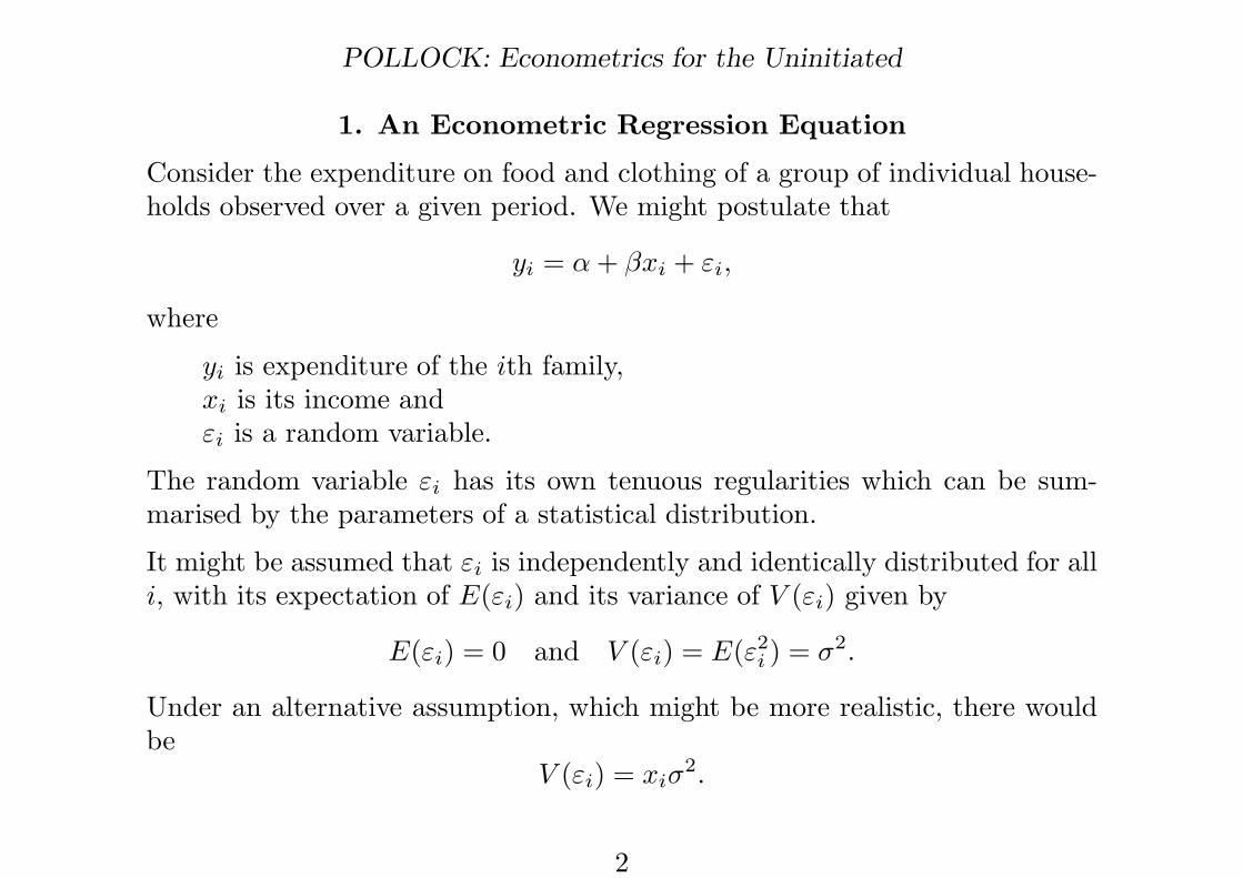
Consider the expenditure on food and clothing of a group of individual house-holds observed over a given period. We might postulate that

yi = α + βxi + εi,

where

yi is expenditure of the ith family,xi is its income andεi is a random variable.

The random variable εi has its own tenuous regularities which can be sum-marised by the parameters of a statistical distribution.

It might be assumed that εi is independently and identically distributed for alli, with its expectation of E(εi) and its variance of V (εi) given by

E(εi) = 0 and V (εi) = E(ε2i ) = σ2.

Under an alternative assumption, which might be more realistic, there wouldbe

V (εi) = xiσ2.

2

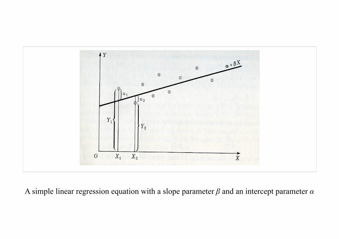
A simple linear regression equation with a slope parameter β and an intercept parameter α


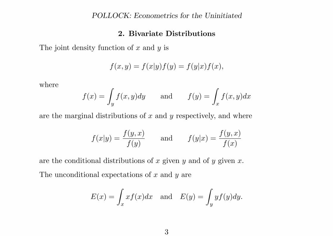
2. Bivariate Distributions

The joint density function of x and y is

f(x, y) = f(x|y)f(y) = f(y|x)f(x),

wheref(x) =

Z

yf(x, y)dy and f(y) =

Z

xf(x, y)dx

are the marginal distributions of x and y respectively, and where

f(x|y) =f(y, x)f(y)

and f(y|x) =f(y, x)f(x)

are the conditional distributions of x given y and of y given x.

The unconditional expectations of x and y are

E(x) =Z

xxf(x)dx and E(y) =

Z

yyf(y)dy.

3

55

60

65

70

75

80

55 60 65 70 75 80

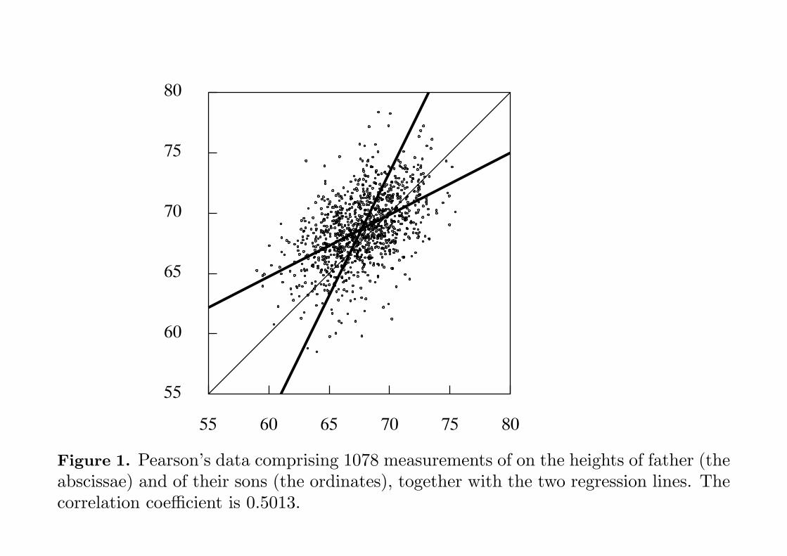
Figure 1. Pearson’s data comprising 1078 measurements of on the heights of father (theabscissae) and of their sons (the ordinates), together with the two regression lines. Thecorrelation coefficient is 0.5013.

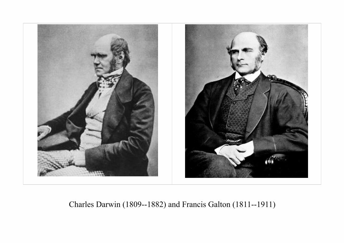
Charles Darwin (1809--1882) and Francis Galton (1811--1911)

The Ascent of Man in a Modern Perspective

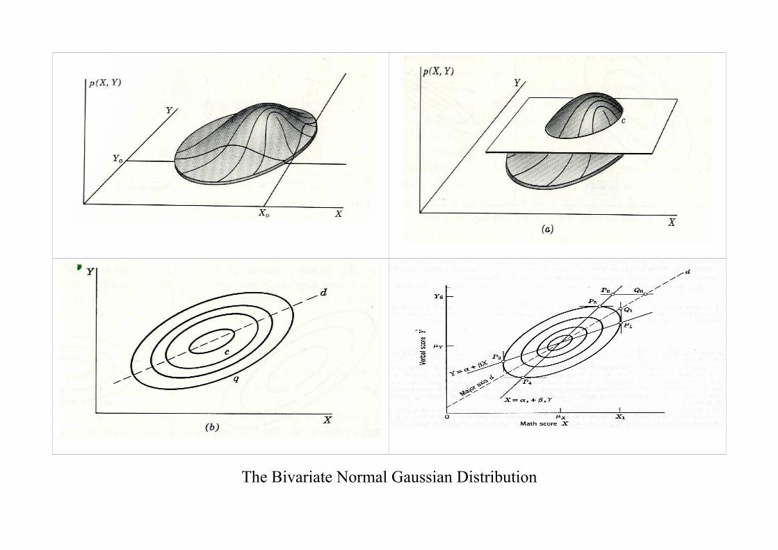
The Bivariate Normal Gaussian Distribution


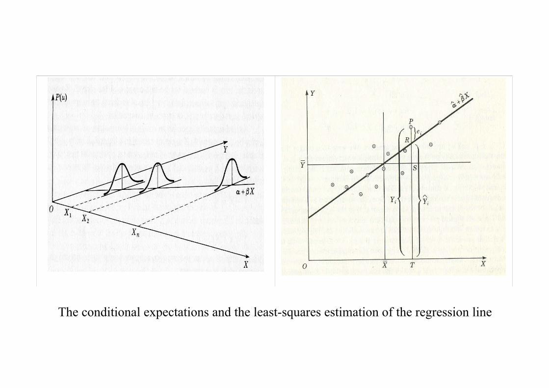
3. Conditional Expectations and Regression

The conditional expectation of y given x is

E(y|x) =Z

yyf(y|x)dy =

Z

yyf(y, x)f(x)

dy.

In the case of the bivariate normal distribution, this constitutes a linearregression:

E(y|x) = E(y) + β{x−E(x)}= {E(y)− βE(x)} + βx

= α + βx.

Here, α = E(y)− βE(x); and it can be shown that

β =C(x, y)V (x)

=E[{x−E(x)}{y −E(y)}]

E[{(x−E(x)}2}

=E(xy)−E(x)E(y)E(x2)− {E(x2)}2

.

4

Images of R.A. Fisher (1890--1962)

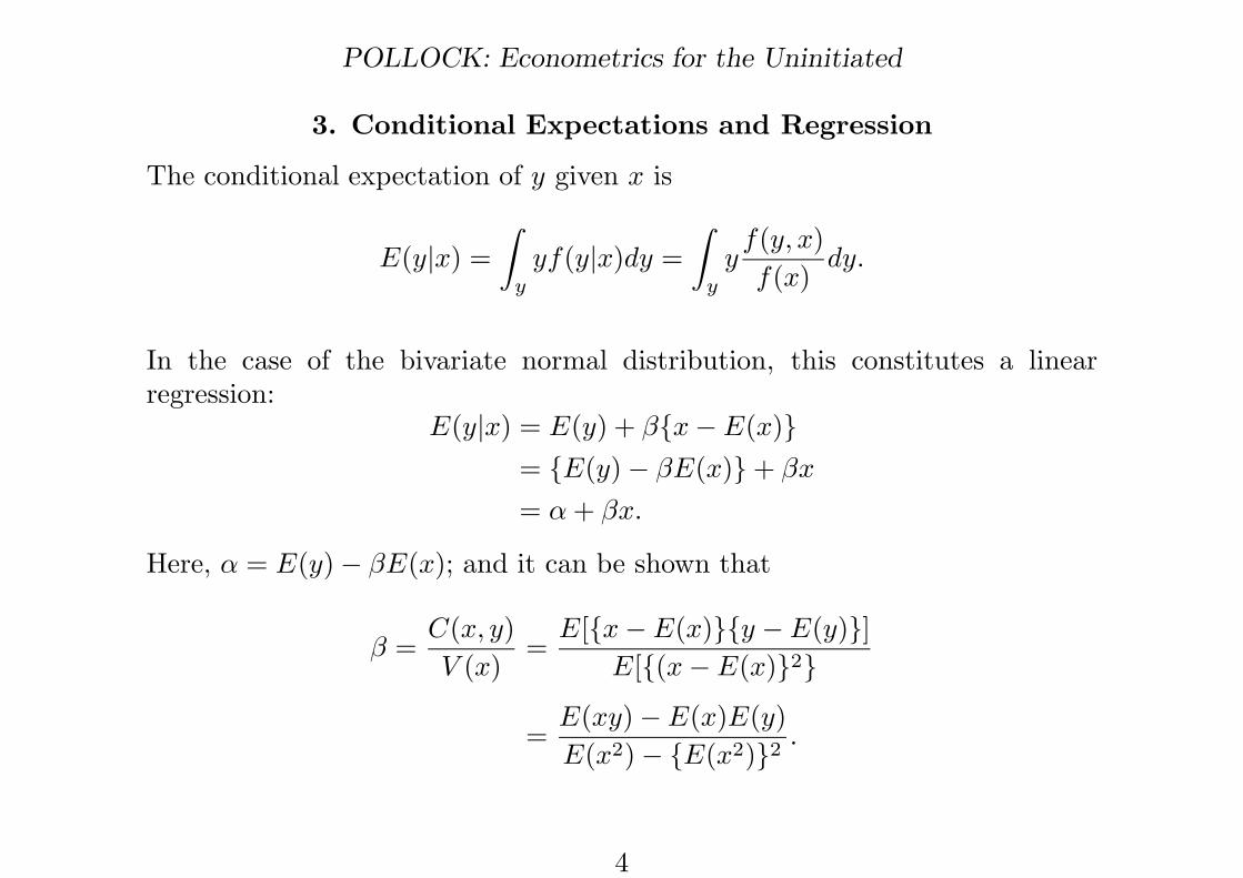
The conditional expectations and the least-squares estimation of the regression line


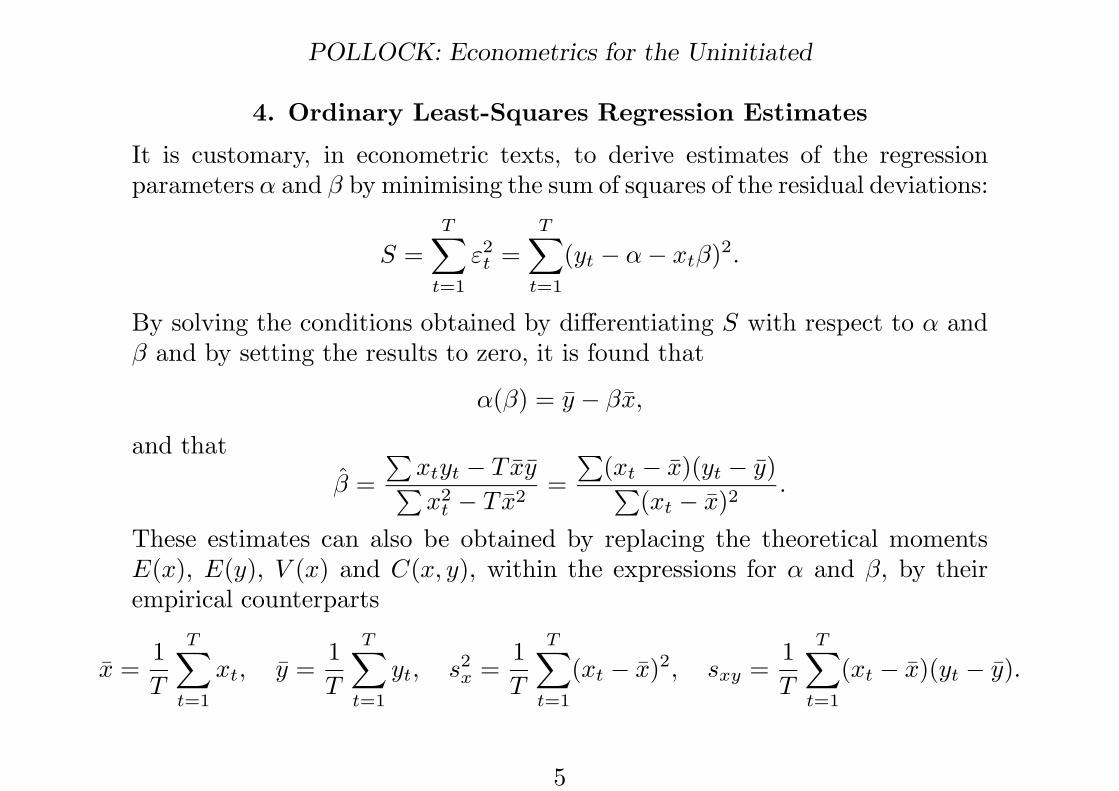
4. Ordinary Least-Squares Regression Estimates

It is customary, in econometric texts, to derive estimates of the regressionparameters α and β by minimising the sum of squares of the residual deviations:

S =TX

t=1

ε2t =

TX

t=1

(yt − α− xtβ)2.

By solving the conditions obtained by differentiating S with respect to α andβ and by setting the results to zero, it is found that

α(β) = y − βx,

and thatβ =

Pxtyt − T xyPx2

t − T x2=

P(xt − x)(yt − y)P

(xt − x)2.

These estimates can also be obtained by replacing the theoretical momentsE(x), E(y), V (x) and C(x, y), within the expressions for α and β, by theirempirical counterparts

x =1T

TX

t=1

xt, y =1T

TX

t=1

yt, s2x =

1T

TX

t=1

(xt − x)2, sxy =1T

TX

t=1

(xt − x)(yt − y).

5

We might as reasonably dispute whether it is the upper or the under blade of a pair of scissors that cuts a piece of paper, as whether value is governed by utility or cost of production.

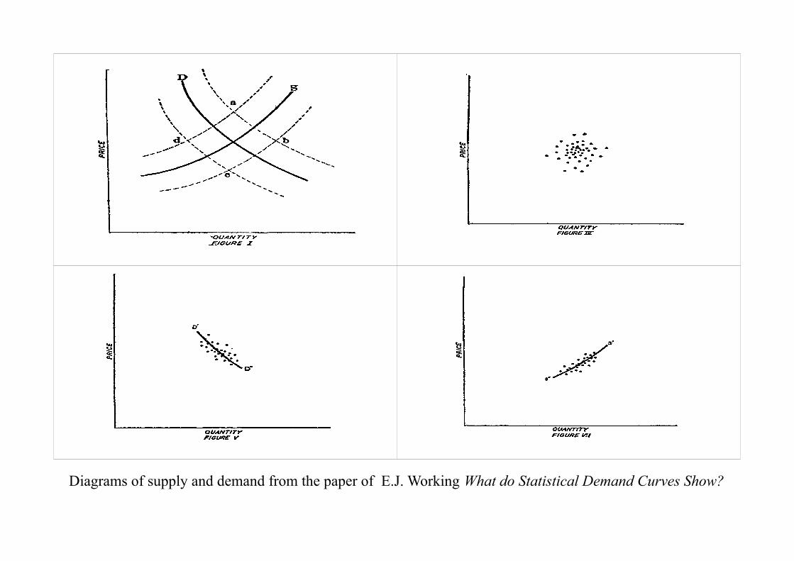
Diagrams of supply and demand from the paper of E.J. Working What do Statistical Demand Curves Show?


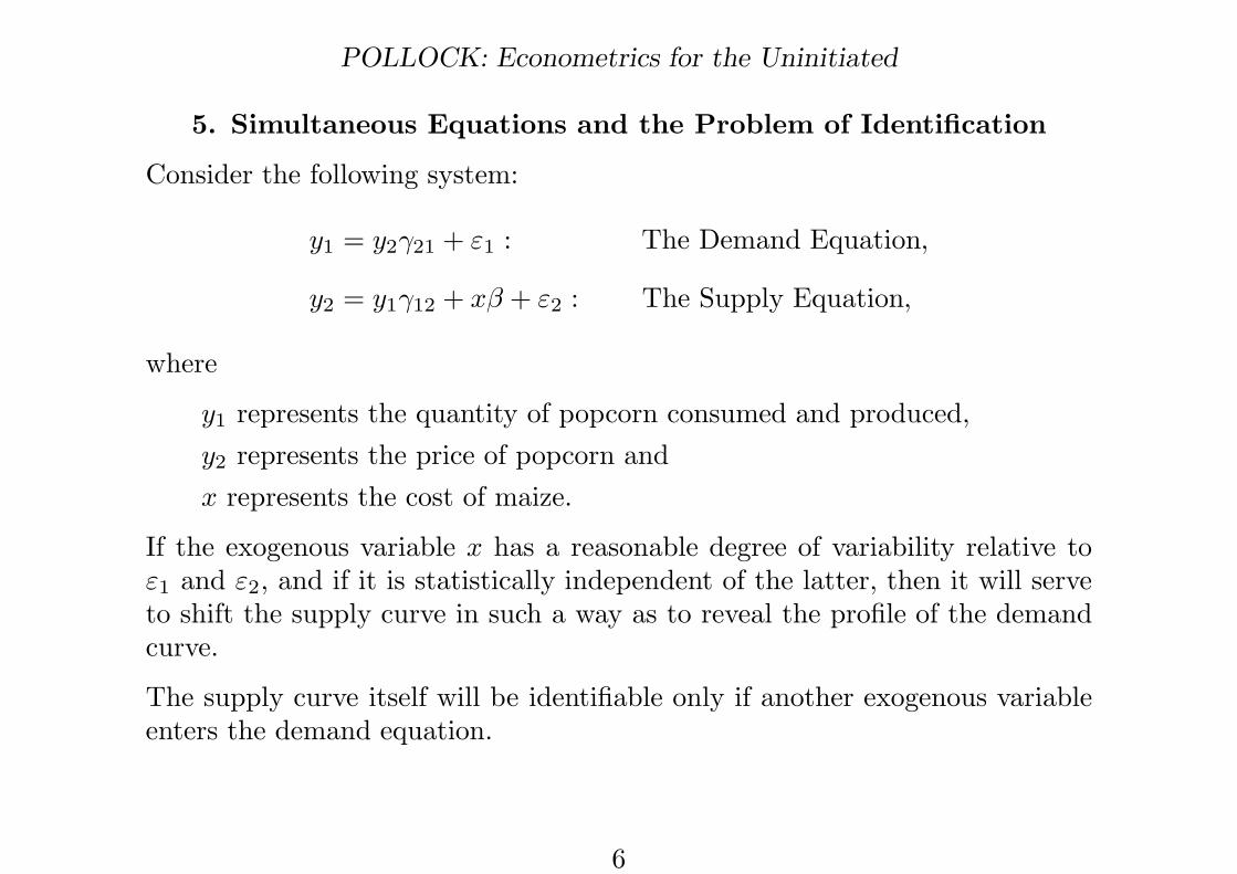
5. Simultaneous Equations and the Problem of Identification

Consider the following system:

y1 = y2γ21 + ε1 : The Demand Equation,

y2 = y1γ12 + xβ + ε2 : The Supply Equation,

where

y1 represents the quantity of popcorn consumed and produced,y2 represents the price of popcorn andx represents the cost of maize.

If the exogenous variable x has a reasonable degree of variability relative toε1 and ε2, and if it is statistically independent of the latter, then it will serveto shift the supply curve in such a way as to reveal the profile of the demandcurve.

The supply curve itself will be identifiable only if another exogenous variableenters the demand equation.

6

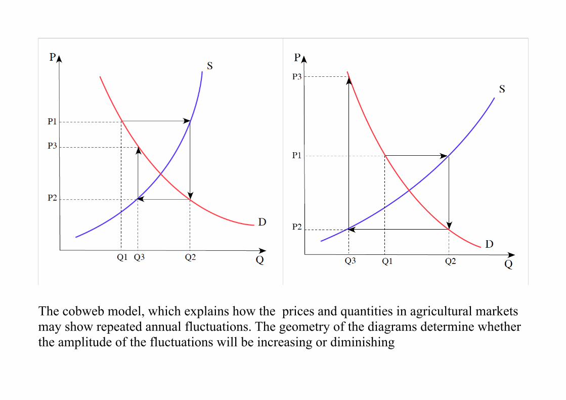
The cobweb model, which explains how the prices and quantities in agricultural markets may show repeated annual fluctuations. The geometry of the diagrams determine whether the amplitude of the fluctuations will be increasing or diminishing


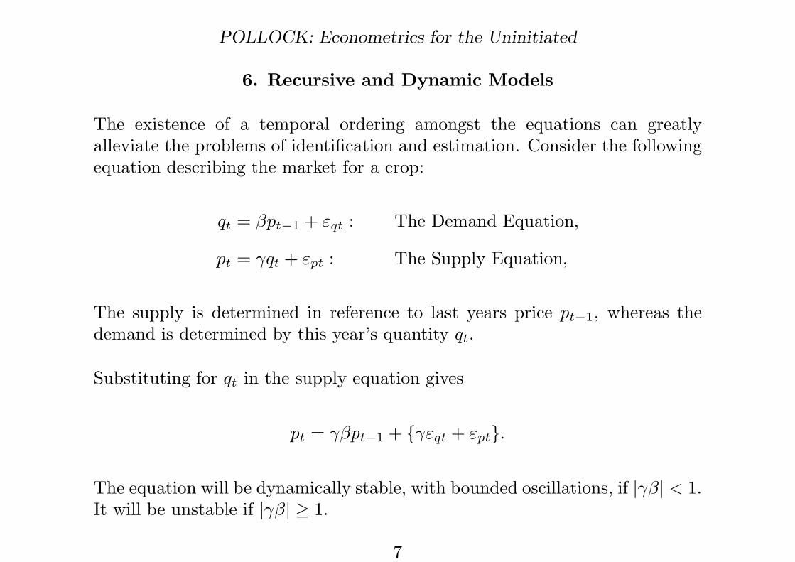
6. Recursive and Dynamic Models

The existence of a temporal ordering amongst the equations can greatlyalleviate the problems of identification and estimation. Consider the followingequation describing the market for a crop:

qt = βpt−1 + εqt : The Demand Equation,

pt = γqt + εpt : The Supply Equation,

The supply is determined in reference to last years price pt−1, whereas thedemand is determined by this year’s quantity qt.

Substituting for qt in the supply equation gives

pt = γβpt−1 + {γεqt + εpt}.

The equation will be dynamically stable, with bounded oscillations, if |γβ| < 1.It will be unstable if |γβ| ≥ 1.

7


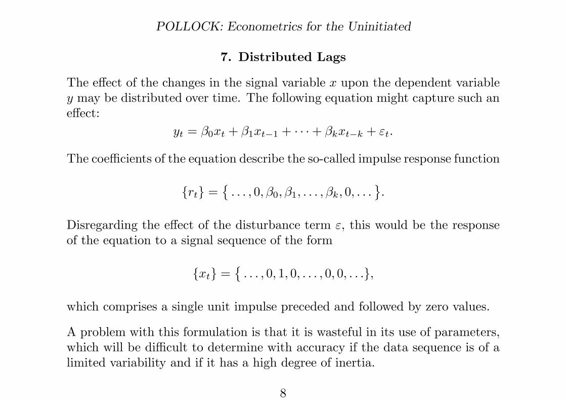
7. Distributed Lags

The effect of the changes in the signal variable x upon the dependent variabley may be distributed over time. The following equation might capture such aneffect:

yt = β0xt + β1xt−1 + · · · + βkxt−k + εt.

The coefficients of the equation describe the so-called impulse response function

{rt} =©

. . . , 0,β0,β1, . . . ,βk, 0, . . .™.

Disregarding the effect of the disturbance term ε, this would be the responseof the equation to a signal sequence of the form

{xt} =©

. . . , 0, 1, 0, . . . , 0, 0, . . .},

which comprises a single unit impulse preceded and followed by zero values.

A problem with this formulation is that it is wasteful in its use of parameters,which will be difficult to determine with accuracy if the data sequence is of alimited variability and if it has a high degree of inertia.

8


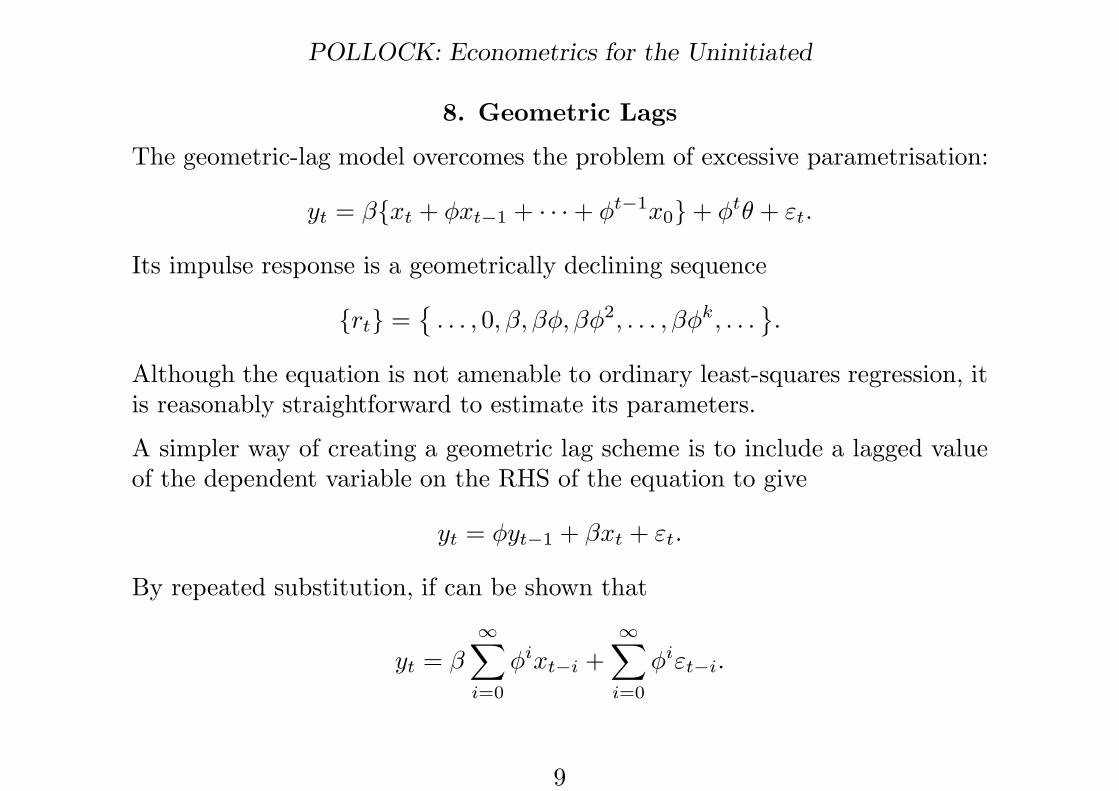
8. Geometric Lags

The geometric-lag model overcomes the problem of excessive parametrisation:

yt = β{xt + φxt−1 + · · · + φt−1x0} + φtθ + εt.

Its impulse response is a geometrically declining sequence

{rt} =©

. . . , 0,β,βφ,βφ2, . . . ,βφk, . . .™.

Although the equation is not amenable to ordinary least-squares regression, itis reasonably straightforward to estimate its parameters.

A simpler way of creating a geometric lag scheme is to include a lagged valueof the dependent variable on the RHS of the equation to give

yt = φyt−1 + βxt + εt.

By repeated substitution, if can be shown that

yt = β∞X

i=0

φixt−i +∞X

i=0

φiεt−i.

9


9. Problems with Trended Variables

Granger and Newbold showed that variables that have a high degree of inertiacan be highly correlated, even when they have been generated independently.Thus, two independent processes

xt = βxt−1 + εt and yt = γyt−1 + ηt

with γ and β close to unity will generate data with a high degree of correlationthat diminishes only gradually as the sample size increases. This creates adanger of spurious regressions.

Equally, if the variable y shows a high degree of inertia, or if it is trended, thena model of the form

yt = φyt−1 + βxt + εt

is liable to fit the data deceptively well, since yt−1 will be close to yt. Suchphenomena have given rise to false claims of success in explaining economicprocesses.

The theory of regression requires the variables to be stationary, which impliesan absence of trend. It is often found that, when the variables are detrended,e.g. by replacing them by their differences∇yt = yt−yt−1 and∇xt = xt−xt−1,the degree of their correlation is radically reduced.

10


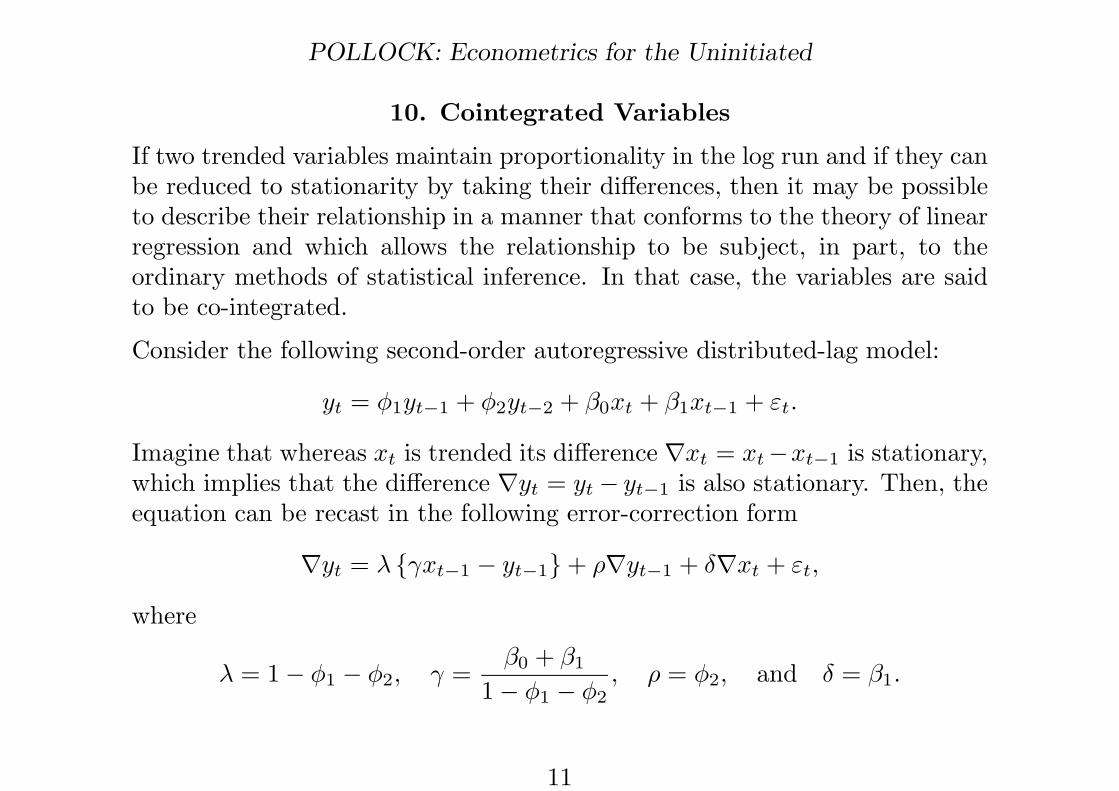
10. Cointegrated Variables

If two trended variables maintain proportionality in the log run and if they canbe reduced to stationarity by taking their differences, then it may be possibleto describe their relationship in a manner that conforms to the theory of linearregression and which allows the relationship to be subject, in part, to theordinary methods of statistical inference. In that case, the variables are saidto be co-integrated.

Consider the following second-order autoregressive distributed-lag model:

yt = φ1yt−1 + φ2yt−2 + β0xt + β1xt−1 + εt.

Imagine that whereas xt is trended its difference ∇xt = xt−xt−1 is stationary,which implies that the difference ∇yt = yt− yt−1 is also stationary. Then, theequation can be recast in the following error-correction form

∇yt = λ {γxt−1 − yt−1} + ρ∇yt−1 + δ∇xt + εt,

where

λ = 1− φ1 − φ2, γ =β0 + β1

1− φ1 − φ2, ρ = φ2, and δ = β1.

11


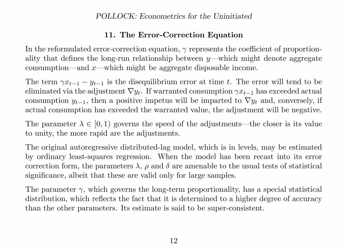
11. The Error-Correction Equation

In the reformulated error-correction equation, γ represents the coefficient of proportion-ality that defines the long-run relationship between y—which might denote aggregateconsumption—and x—which might be aggregate disposable income.

The term γxt−1 − yt−1 is the disequilibrium error at time t. The error will tend to beeliminated via the adjustment∇yt. If warranted consumption γxt−1 has exceeded actualconsumption yt−1, then a positive impetus will be imparted to ∇yt and, conversely, ifactual consumption has exceeded the warranted value, the adjustment will be negative.

The parameter λ ∈ [0, 1) governs the speed of the adjustments—the closer is its valueto unity, the more rapid are the adjustments.

The original autoregressive distributed-lag model, which is in levels, may be estimatedby ordinary least-squares regression. When the model has been recast into its errorcorrection form, the parameters λ, ρ and δ are amenable to the usual tests of statisticalsignificance, albeit that these are valid only for large samples.

The parameter γ, which governs the long-term proportionality, has a special statisticaldistribution, which reflects the fact that it is determined to a higher degree of accuracythan the other parameters. Its estimate is said to be super-consistent.

12

Documents

Econometrics for the Uninitiated - University of Leicester