Embed Size (px)
Citation preview

Econometrics Basics: Investigating the
Stationarity of Time Series
John E. FloydUniversity of Toronto
July 22, 2013
It is often useful to think of a time series as a sequence of numbers generatedby some mathematical process and to attempt to determine which processbest describes the behavior of that series.1 For example, a particular seriesmight be generated according to the equation
yt = β yt−1 + ϵt (1)
where yt is the level of the series at time t and ϵt is a series of drawingsof a zero-mean, constant-variance non-autocorrelated random variable. Theabove equation is a first-order autoregressive process—first order becausethere is one lag of yt on the right-hand side and autoregressive because theyt are autocorrelated in the sense that the level of the variable in a particularperiod depends on its level in one or more previous periods.
Lagging the above equation repeatedly and substituting these lags backinto (1) produces the expression
yt = β t y0 + ϵt + β ϵt−1 + β2ϵt−2 + β3 ϵt−3
+β4 ϵt−4 + · · · · · · · · ·+ β t ϵ0. (2)
The time path of yt depends critically on the parameter β. If this parameterequals zero then
yt = ϵt. (3)
1A very basic discussion of time series analysis can be found in Walter Enders, AppliedTime Series Analysis, John Wiley and Sons, 1995. For a deeper analysis, see JamesHamilton, Time Series Analysis, Princeton University Press, 1994.
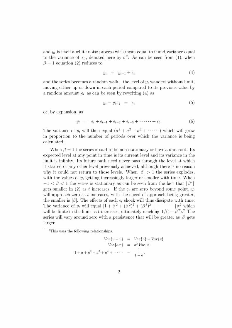
and yt is itself a white noise process with mean equal to 0 and variance equalto the variance of ϵt , denoted here by σ2. As can be seen from (1), whenβ = 1 equation (2) reduces to
yt = yt−1 + ϵt (4)
and the series becomes a random walk—the level of yt wanders without limit,moving either up or down in each period compared to its previous value bya random amount ϵt as can be seen by rewriting (4) as
yt − yt−1 = ϵt (5)
or, by expansion, as
yt = ϵt + ϵt−1 + ϵt−2 + ϵt−3 + · · · · · ·+ ϵ0. (6)
The variance of yt will then equal (σ2 + σ2 + σ2 + · · · · · ·) which will growin proportion to the number of periods over which the variance is beingcalculated.
When β = 1 the series is said to be non-stationary or have a unit root. Itsexpected level at any point in time is its current level and its variance in thelimit is infinity. Its future path need never pass through the level at whichit started or any other level previously achieved, although there is no reasonwhy it could not return to those levels. When |β| > 1 the series explodes,with the values of yt getting increasingly larger or smaller with time. When−1 < β < 1 the series is stationary as can be seen from the fact that | β t|gets smaller in (2) as t increases. If the ϵt are zero beyond some point, ytwill approach zero as t increases, with the speed of approach being greater,the smaller is |β|. The effects of each ϵt shock will thus dissipate with time.The variance of yt will equal [1 + β 2 + (β 2)2 + (β 3)2 + · · · · · · · · ·]σ2 whichwill be finite in the limit as t increases, ultimately reaching 1/(1−β 2).2 Theseries will vary around zero with a persistence that will be greater as β getslarger.
2This uses the following relationships.
Var{u+ v} = Var{u}+ Var{v}Var{a x} = a2 Var{x}
1 + a+ a2 + a3 + a4 + · · · · · · =1
1− a.
2
Equation (1) is a first-order autoregressive process. An autoregressiveprocess of second-order would be represented by
yt = β1 yt−1 + β2 yt−2 + ϵt, (7)
with two lags of yt, and third and higher order processes simply inolve theaddition of further lags.
Time series can also be moving average processes such as, for example,
yt = ξ0 ϵt + ξ1 ϵt−1 + ξ2 ϵt−2 (8)
which is a second-order moving average process—second-order because itcontains two lags of the error term. Moving average processes are alwaysstationary because ϵt is stationary and any average of stationary processesmust itself be a stationary process.
Of course, time series processes can have both autoregressive and movingaverage components as in the expression
yt = β1 yt−1 + β2 yt−2 + ξ0 ϵt + ξ1 ϵt−1 + ξ2 ϵt−2 (9)
which defines an ARMA(2,2) process—a process that is second-order autore-gressive and second-order moving average. In general, ARMA(p, q) processeshave p autoregressive lags and q moving average lags.
It is possible that yt above could be a stationary process that is actuallythe first difference of another series, yt = zt−zt−1, where zt is a non-stationaryautoregressive moving average process that has to be differenced once toproduce the stationary ARMA(2,2) process. It is said to be integrated oforder 1 because it has to be differenced once to produce a stationary process.If it had to be differenced twice to produce a stationary process it wouldbe integrated of order 2, and so forth. The process zt is thus an auto-regressive-integrated-moving-average ARIMA(2,1,2) process—differencing itonce produces an ARMA(2,2) process. In general, an ARIMA(p, d, q) processis one whose d-th difference is a stationary autoregressive-moving-averageprocess with p autoregressive lags and q moving average lags.
3
Subtraction of yt−1 from both sides of (9) converts it to
yt − yt−1 = −(1− β1) yt−1 + β2 yt−2
+ ξ0 ϵt + ξ1 ϵt−1 + ξ2 ϵt−2 (10)
and a further addition and subtraction of β2 yt−1 on the right side yields
yt − yt−1 = −(1− β1 − β2) yt−1 + β2 (yt−2 − yt−1)
+ ξ0 ϵt + ξ1 ϵt−1 + ξ2 ϵt−2. (11)
This series will be stationary as long as β1 + β2 < 1 so that a fraction(1− β1 − β2) of any change in yt will be removed in each subsequent period.A random-walk will only occur if β1 + β2 = 1 , in which case expressionreduces to
yt − yt−1 = ξ0 ϵt + ξ1 ϵt−1 + ξ2 ϵt−2 (12)
and any change in yt from period to period will be permanent.
It turns out that an equation like (9) that includes autoregressive andmoving-average terms can be expressed in the form of a pure autoregressiveprocess containing an infinite number of autoregressive lags.3 Simply reor-ganize (9) to move ϵt to the left of the equality and yt to the right, lag theresulting equation repeatedly to obtain expressions for et−1, et−2, et−3 . . .etc. and substitute these expressions successively into (9) and simplify. Theresulting infinite order autoregressive process can then be converted into anequation like
∆yt = −(1− ρ) yt−1 + (β2 + β3 + β4 + · · ·+ β∞)∆yt−1
+(β3 + β4 + · · ·+ β∞)∆yt−2
+(β4 + · · ·+ β∞)∆yt−3 + · · · · · · · · ·+ ϵt (13)
containing an infinite succession of lags of ∆yt = (yt − yt−1) where thestationarity parameter ρ = β1 + β2 + β3 + · · · · · · + β∞. Stationarity occurswhere ρ < 1 and therefore −(1− ρ) < 0 .
3See pages 225–227 of the book by Enders.
4
Our econometric problem here is to determine whether the time-seriesprocesses that can reasonably describe the evolution of particular time-seriesvariables are stationary. The standard procedure, based on path-breakingwork by Dickey and Fuller4 is to perform a Dickey-Fuller Test which usesordinary-least-squares to estimate an equation of the form
∆qt = α+ γ t− (1− ρ) qt−1 + δ1 ∆qt−1 + δ2 ∆qt−2
+ δ3 ∆qt−3 + · · · · · · · · ·+ ϵt (14)
which is equivalent to the infinite autoregressive process discussed above withthe addition of a constant term and trend. It turns out that, under the nullhypothesis that there is no mean reversion and ρ = 1, this process can be wellapproximated by an AR process containing no more than T 1/3 lags, where Tis the number of observations. The deterministic terms α and γ t are droppedif there is no evidence of a trend in the series—if α is significantly differentfrom zero, the rejection of the null-hypothesis of ρ = 1 indicates stationarityof the series around a drift or trend and if γ is significantly different fromzero the series is stationary around an increasing or decreasing drift or trend.Two equations additional to the one above are estimated, one without γ tand a second without α+ γ t .
∆qt = α− (1− ρ) qt−1 + δ1 ∆qt−1 + δ2 ∆qt−2
+ δ3 ∆qt−3 + · · · · · · · · ·+ ϵt (15)
∆qt = − (1− ρ) qt−1 + δ1 ∆qt−1 + δ2 ∆qt−2
+ δ3 ∆qt−3 + · · · · · · · · ·+ ϵt . (16)
In selecting the number of lags to be included, an appropriate procedureis to start with an unreasonably large number and progressively drop thelongest lag if that lag turns out to be statistically insignificant. An alternativeis to choose the number of lags that minimizes an information criterion suchas the Akaike information criterion (AIC) or Schwartz Bayesian informationcriterion (SBC). These give calculated optimal balances between the gainassociated with the reduction in the residual sum of squares when a lag is
4David Dickey and Wayne A. Fuller, “Distribution of the Estimates for AutoregressiveTime Series with a Unit Root,” Journal of the American Statistical Association Vol. 74,June 1979, 427-431, and “Likelihood Ratio Statistics for Autoregressive Time Series witha Unit Root,” Econometrica Vol. 49, July 1981, 1957-72.
5

added and the loss associated with having one less degree of freedom. Therelevant formulae to be calculated for each regression are
AIC(n) = ln
(SSR(n)
T
)+ (n+ 1)
2
T(17)
SBC(n) = ln
(SSR(n)
T
)+ (n+ 1)
ln(T )
T(18)
were SSR(n) is the sum of squared residuals, n is the number of lags andT is the number of observations and where ln() is represents the naturallogarithm of the expression in the brackets.5 Of course, all these significancetests and criteria comparisons must apply to regressions estimated from thesame number of observations.
It turns out that under the null-hypothesis that ρ = 1 the estimator of(1− ρ) is not distributed according to the t-distribution. A table of criticalvalues constructed by Dickey and Fuller must be used instead of the standardt-tables.6
Our first task in writing a function in XLispStat to do Dickey-Fullertests is to develop an easy method of deciding how many lags to use. To dothis, we construct a DFlags function. As a prelude to this, we modify ourmakelags function very slightly, inserting the word lagmat on a line by itselfat the very end of the function.
) ; end of dotimes
lagmat
) ; end of function
This code line makes the matrix lagmat the designated output of the func-tion, rather than just one of a number of objects left in the workspace. As aresult, we can use the def function to give it another name as follows.
(def newmatrix (makelags 5 variable))
5See James H. Stock and Mark W. Watson, Introduction to Econometrics, AddisonWesley, 2003, pages 453–467, for a discussion of these criteria. The authors recommendthe AIC over the SBC for the purpose at hand because the former tends to overestimatethe number of lags and studies of the performance of Dickey-Fuller tests suggest thathaving too many lags is better than having too few.
6A collection of these and other tables can be found in the file statabs.pdf.
6

We now construct our function to aid in deciding the number of lags topass to the Dickey-Fuller unit root function we will subsequently construct.The argument y is the variable we are checking for stationarity and theargument m denotes the maximum allowable number of lags. We also use theregression-model function provided by XLispStat instead of our runOLSfunction in both of the new functions we create.
(defun DFlags (y m)
"Args: (y m)
Provides information to enable us to decide how many lags to use in a
subsequent Dickey-Fuller unit root test of the series y starting with
a maximum lag m. The AIC and SBC statistics are expressed as fractions
of the levels that resulted with the maximum lag."
(def dimlist (list (+ m 2) m))
Our first line of code above creates a list giving the dimensions of the matrixwe will construct to contain the P-Values of the lags in a series of regressionsstarting with a lag of m and sequentially reducing the number of lags by oneuntil only a single lag remains. This matrix will have along the top of it theAIC and SBC values associated with each of the regressions. We now makethe shell of that matrix, into which the proper values will be later inserted,together with a list that will represent its first (left-most) column.
(def bigmat (make-array dimlist :initial-element " "))
(def col1list (combine "AIC" "BIC" (iseq 1 m)))
(def lagy (remove-last 1 y))
(def diffy (- (remove-first 1 y)(remove-last 1 y)))
(def lagmat (makelags m diffy))
(def lagy (remove-first m lagy))
(def diffy (select lagslist 0))
The last five lines of code above create the first difference of the variable towhich we are going to apply our Dickey-Fuller test, then set up a matrix of themaximum number of lags of ∆y, and finally, the two series representing thecurrent values of ∆y and yt−1 with lengths appropriate for the regressionsthat will follow. We then run the first regression (the one with the mostlags) in the first code line below and in the subsequent four lines of codeextract the t-ratios and calculate the P-values of the lags and then calculatethe values of the AIC and SBC for this first regression.
7
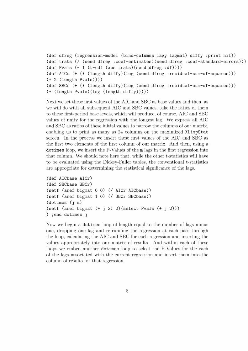
(def dfreg (regression-model (bind-columns lagy lagmat) diffy :print nil))
(def trats (/ (send dfreg :coef-estimates)(send dfreg :coef-standard-errors)))
(def Pvals (- 1 (t-cdf (abs trats)(send dfreg :df))))
(def AICr (+ (* (length diffy)(log (send dfreg :residual-sum-of-squares)))
(* 2 (length Pvals))))
(def SBCr (+ (* (length diffy)(log (send dfreg :residual-sum-of-squares)))
(* (length Pvals)(log (length diffy)))))
Next we set these first values of the AIC and SBC as base values and then, aswe will do with all subsequent AIC and SBC values, take the ratios of themto these first-period base levels, which will produce, of course, AIC and SBCvalues of unity for the regression with the longest lag. We express all AICand SBC as ratios of these initial values to narrow the columns of our matrix,enabling us to print as many as 24 columns on the maximized XLispStat
screen. In the process we insert these first values of the AIC and SBC asthe first two elements of the first column of our matrix. And then, using adotimes loop, we insert the P-Values of the m lags in the first regression intothat column. We should note here that, while the other t-statistics will haveto be evaluated using the Dickey-Fuller tables, the conventional t-statisticsare appropriate for determining the statistical significance of the lags.
(def AICbase AICr)
(def SBCbase SBCr)
(setf (aref bigmat 0 0) (/ AICr AICbase))
(setf (aref bigmat 1 0) (/ SBCr SBCbase))
(dotimes (j m)
(setf (aref bigmat (+ j 2) 0)(select Pvals (+ j 2)))
) ;end dotimes j
Now we begin a dotimes loop of length equal to the number of lags minusone, dropping one lag and re-running the regression at each pass throughthe loop, calculating the AIC and SBC for each regression and inserting thevalues appropriately into our matrix of results. And within each of theseloops we embed another dotimes loop to select the P-Values for the eachof the lags associated with the current regression and insert them into thecolumn of results for that regression.
8
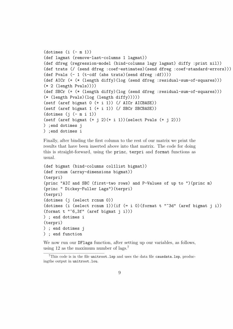
(dotimes (i (- m 1))
(def lagmat (remove-last-columns 1 lagmat))
(def dfreg (regression-model (bind-columns lagy lagmat) diffy :print nil))
(def trats (/ (send dfreg :coef-estimates)(send dfreg :coef-standard-errors)))
(def Pvals (- 1 (t-cdf (abs trats)(send dfreg :df))))
(def AICr (+ (* (length diffy)(log (send dfreg :residual-sum-of-squares)))
(* 2 (length Pvals))))
(def SBCr (+ (* (length diffy)(log (send dfreg :residual-sum-of-squares)))
(* (length Pvals)(log (length diffy)))))
(setf (aref bigmat 0 (+ i 1)) (/ AICr AICBASE))
(setf (aref bigmat 1 (+ i 1)) (/ SBCr SBCBASE))
(dotimes (j (- m i 1))
(setf (aref bigmat (+ j 2)(+ i 1))(select Pvals (+ j 2)))
) ;end dotimes j
) ;end dotimes i
Finally, after binding the first column to the rest of our matrix we print theresults that have been inserted above into that matrix. The code for doingthis is straight-forward, using the princ, terpri and format functions asusual.
(def bigmat (bind-columns col1list bigmat))
(def rcnum (array-dimensions bigmat))
(terpri)
(princ "AIC and SBC (first-two rows) and P-Values of up to ")(princ m)
(princ " Dickey-Fuller Lags")(terpri)
(terpri)
(dotimes (j (select rcnum 0))
(dotimes (i (select rcnum 1))(if (= i 0)(format t "~3d" (aref bigmat j i))
(format t "~6,3f" (aref bigmat j i)))
) ; end dotimes i
(terpri)
) ; end dotimes j
) ; end function
We now run our DFlags function, after setting up our variables, as follows,using 12 as the maximum number of lags.7
7This code is in the file unitroot.lsp and uses the data file causdata.lsp, produc-ingthe output in unitroot.lou.
9
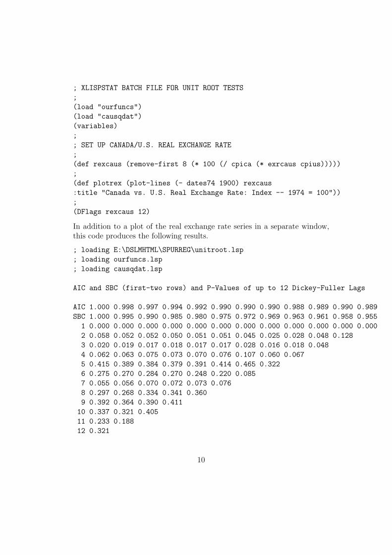
; XLISPSTAT BATCH FILE FOR UNIT ROOT TESTS
;
(load "ourfuncs")
(load "causqdat")
(variables)
;
; SET UP CANADA/U.S. REAL EXCHANGE RATE
;
(def rexcaus (remove-first 8 (* 100 (/ cpica (* exrcaus cpius)))))
;
(def plotrex (plot-lines (- dates74 1900) rexcaus
:title "Canada vs. U.S. Real Exchange Rate: Index -- 1974 = 100"))
;
(DFlags rexcaus 12)
In addition to a plot of the real exchange rate series in a separate window,this code produces the following results.
; loading E:\DSLMHTML\SPURREG\unitroot.lsp
; loading ourfuncs.lsp
; loading causqdat.lsp
AIC and SBC (first-two rows) and P-Values of up to 12 Dickey-Fuller Lags
AIC 1.000 0.998 0.997 0.994 0.992 0.990 0.990 0.990 0.988 0.989 0.990 0.989
SBC 1.000 0.995 0.990 0.985 0.980 0.975 0.972 0.969 0.963 0.961 0.958 0.955
1 0.000 0.000 0.000 0.000 0.000 0.000 0.000 0.000 0.000 0.000 0.000 0.000
2 0.058 0.052 0.052 0.050 0.051 0.051 0.045 0.025 0.028 0.048 0.128
3 0.020 0.019 0.017 0.018 0.017 0.017 0.028 0.016 0.018 0.048
4 0.062 0.063 0.075 0.073 0.070 0.076 0.107 0.060 0.067
5 0.415 0.389 0.384 0.379 0.391 0.414 0.465 0.322
6 0.275 0.270 0.284 0.270 0.248 0.220 0.085
7 0.055 0.056 0.070 0.072 0.073 0.076
8 0.297 0.268 0.334 0.341 0.360
9 0.392 0.364 0.390 0.411
10 0.337 0.321 0.405
11 0.233 0.188
12 0.321
10
The maximum number of significant lags is three and, it turns out, the AICis almost minimized with that number of lags and with one lag (although theminimum is with four lags), while the SBC is minimized with one lag.
Another way to decide how many lags to use is to examine the statisticalsignificance of the autocorrelations and partial-autocorrelations of the firstdifference of the time-series variable, being tested for stationarity. For doingthis we develop a function called acfpacf. The econometrics underlyingthis function is quite complicated—it is insufficient to simply calculate thecorrelations between the current and all lagged values of the series to obtainthe autocorrelations and to run a single OLS regression including all laggedvalues to obtain the partial-autocorrelations. The standard approach, whichis outlined by Davidson and MacKinnon in their graduate-level textbook, isto calculate the jth autocorrelation as the covariance of the jth lag of thevariable with its current level divided by the variance of the current level.8
ρ (j) =Cov(yt, yt−j)
Var(yt)(19)
where
Cov(yt, yt−j) =1
n− 1
n∑t=j+1
(yt − y)(yt−j − y) (20)
and
Var(yt) =1
n− 1
n∑t=1
(yt − y)2 . (21)
The function Cov( ) defines the covariance of the two time-series in thebrackets and the function Var( ) defines the variance of the single seriesin the brakets. In a standard calculation of a correlation coefficient, thedenominator of (19) would equal the product of the standard-deviations ofthe two time series in the numerator rather than the variance of one of them.And the number of elements summed in (20) is less than the number summedin (21) by an amount equal to the number of lags involved in the calculationof each particular element, or correlation coefficient, in the autocorrelationfunction. But the calculations in the above equations make good sense when
8Russell Davidson and James G. MacKinnon, Econometric Theory and Methods, Ox-ford University Press, 2004, pages 564 and 565.
11
we note that the purpose of calculating these autocorrelations is to see ifwe can reject the null-hypotheses that they are zero—lags included in ourdfunit function will equal the set of lags up to the the longest statisticallysignificant one. Under the null-hypothesis that there are no correlationsbetween the lags, the expected variances, and therefore standard deviations,of the current series and all lags of that series should be the same in a largeenough sample. Hence, the square-root of the variance of the entire unlaggedseries will give the best estimate of the standard deviations of all lags of thatseries. And the variance of the entire unlagged series will thus give the bestestimate of the product of the standard deviations of the series and any ofits lags. It is also desirable to use the maximum possible number of elementsin calculating each of the covariances, taking account of the fact that in thenumerator of (19) the creation of lags uses up, in each case, a number ofelements equal to the length of the longest lag.
The reason why we need to examine the partial correlations is that, forexample, the fourth lag will be correlated with the unlagged series becauseits level will be determined in part by the level of the thrice-lagged series,which will be determined in part by the level of the twice-lagged series,which will be determined in part by level of the the once-lagged series, evenif only the first lag is statistically significant in regressions of the series onits first four lags. However, we do not want to determine the statisticalsignificance of, say, the third lag of a series by regressing the series on thefirst ten of its lags because lags longer than three should not be allowed toinfluence the coefficients of the first three lags, as they might well do, becausea decision to use three lags must be based on the statistical significanceof those three lags, uncontaminated by the effects of adding further lagswhich, themselves, might not be statistically significant. Accordingly, thepartial-autocorrelation function—that is the list of partial-autocorrelations—must be obtained by regressing the current level of the series on one lagand then using the coefficient of that lag as a measure of the first partial-autocorrelation and then adding additional lags in sequence, measuring thepartial-autocorrelation of each of these lags by its coefficient when it is thelongest lag. To calculate twelve partial-autocorrelations, therefore, we haveto run twelve regressions, starting with one lag and adding additional lags inturn, recording in each case the coefficient of the added lag.
A final issue is the setting of confidence limits beyond which the null-hypotheses of zero autocorrelation and partial-autocorrelation can be re-
12
jected. Here we utilize the fact that the variance of each correlation is equalto 1/T where T is the number of observations. A two-tailed 5% confidenceinterval can thus be obtained by taking the square root of 1/T to obtain thestandard deviation and then multiplying that standard deviation by 2 andassigning to the result both positive and negative values.9
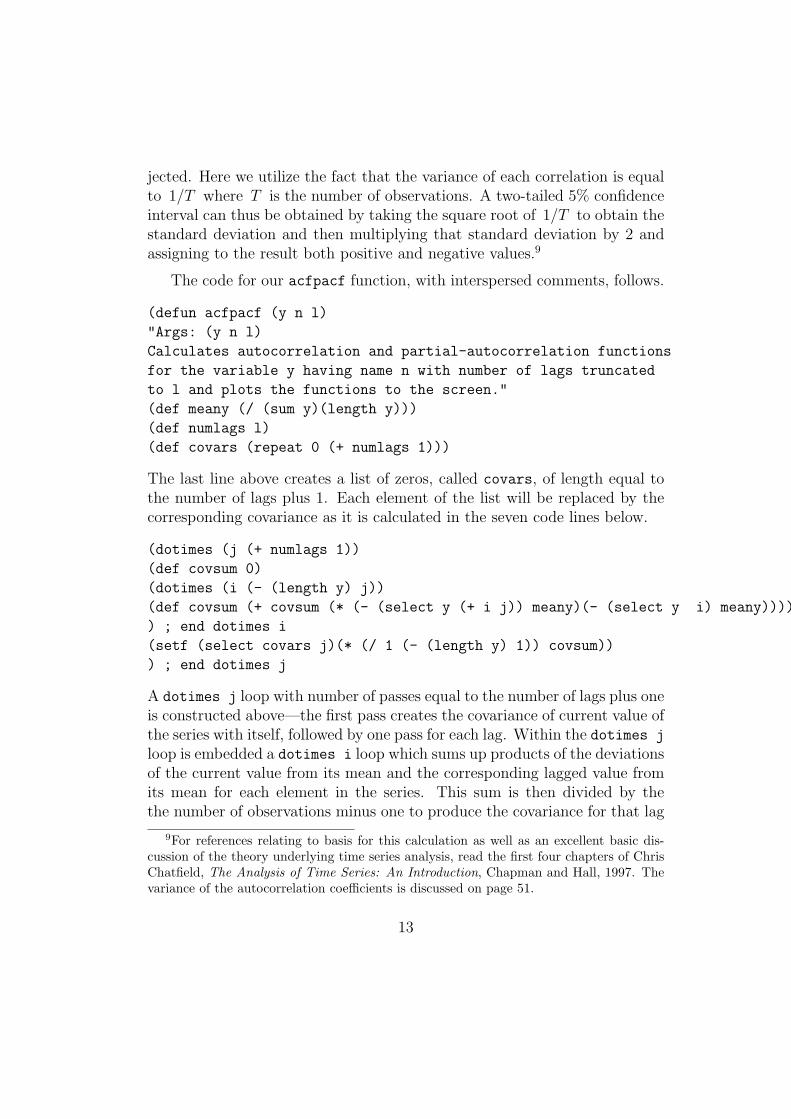
The code for our acfpacf function, with interspersed comments, follows.
(defun acfpacf (y n l)
"Args: (y n l)
Calculates autocorrelation and partial-autocorrelation functions
for the variable y having name n with number of lags truncated
to l and plots the functions to the screen."
(def meany (/ (sum y)(length y)))
(def numlags l)
(def covars (repeat 0 (+ numlags 1)))
The last line above creates a list of zeros, called covars, of length equal tothe number of lags plus 1. Each element of the list will be replaced by thecorresponding covariance as it is calculated in the seven code lines below.
(dotimes (j (+ numlags 1))
(def covsum 0)
(dotimes (i (- (length y) j))
(def covsum (+ covsum (* (- (select y (+ i j)) meany)(- (select y i) meany))))
) ; end dotimes i
(setf (select covars j)(* (/ 1 (- (length y) 1)) covsum))
) ; end dotimes j
A dotimes j loop with number of passes equal to the number of lags plus oneis constructed above—the first pass creates the covariance of current value ofthe series with itself, followed by one pass for each lag. Within the dotimes j
loop is embedded a dotimes i loop which sums up products of the deviationsof the current value from its mean and the corresponding lagged value fromits mean for each element in the series. This sum is then divided by thethe number of observations minus one to produce the covariance for that lag
9For references relating to basis for this calculation as well as an excellent basic dis-cussion of the theory underlying time series analysis, read the first four chapters of ChrisChatfield, The Analysis of Time Series: An Introduction, Chapman and Hall, 1997. Thevariance of the autocorrelation coefficients is discussed on page 51.
13
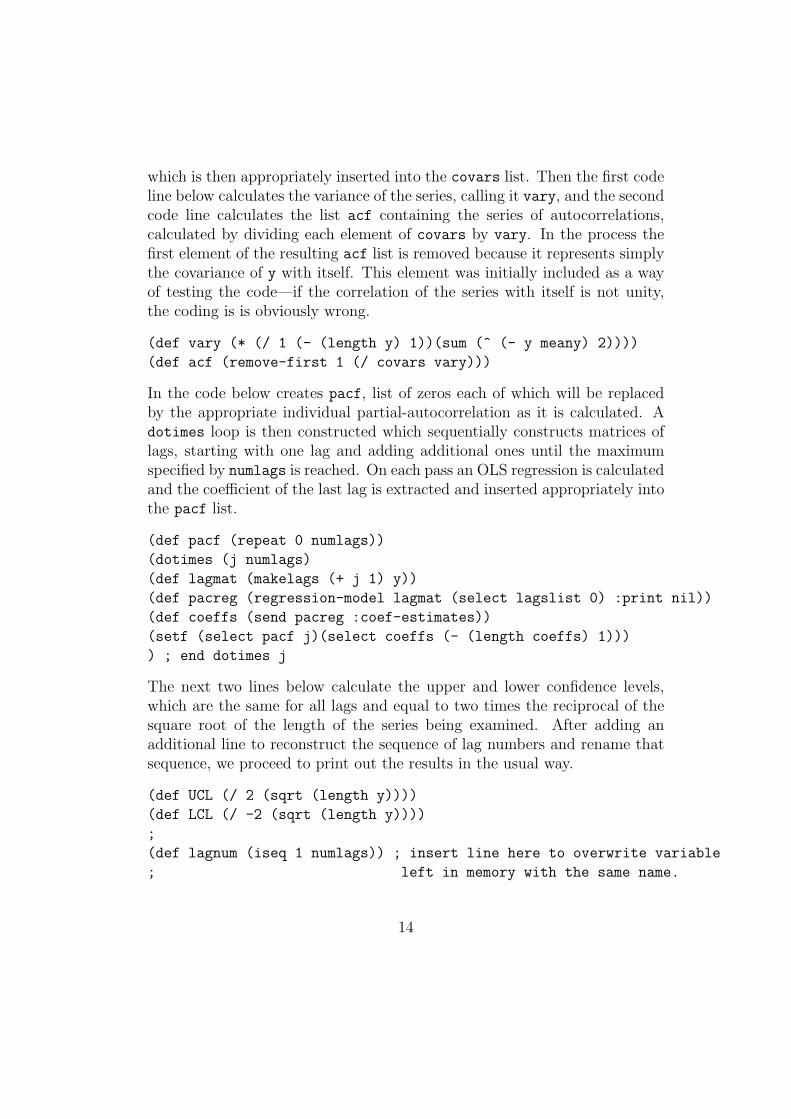
which is then appropriately inserted into the covars list. Then the first codeline below calculates the variance of the series, calling it vary, and the secondcode line calculates the list acf containing the series of autocorrelations,calculated by dividing each element of covars by vary. In the process thefirst element of the resulting acf list is removed because it represents simplythe covariance of y with itself. This element was initially included as a wayof testing the code—if the correlation of the series with itself is not unity,the coding is is obviously wrong.
(def vary (* (/ 1 (- (length y) 1))(sum (^ (- y meany) 2))))
(def acf (remove-first 1 (/ covars vary)))
In the code below creates pacf, list of zeros each of which will be replacedby the appropriate individual partial-autocorrelation as it is calculated. Adotimes loop is then constructed which sequentially constructs matrices oflags, starting with one lag and adding additional ones until the maximumspecified by numlags is reached. On each pass an OLS regression is calculatedand the coefficient of the last lag is extracted and inserted appropriately intothe pacf list.
(def pacf (repeat 0 numlags))
(dotimes (j numlags)
(def lagmat (makelags (+ j 1) y))
(def pacreg (regression-model lagmat (select lagslist 0) :print nil))
(def coeffs (send pacreg :coef-estimates))
(setf (select pacf j)(select coeffs (- (length coeffs) 1)))
) ; end dotimes j
The next two lines below calculate the upper and lower confidence levels,which are the same for all lags and equal to two times the reciprocal of thesquare root of the length of the series being examined. After adding anadditional line to reconstruct the sequence of lag numbers and rename thatsequence, we proceed to print out the results in the usual way.
(def UCL (/ 2 (sqrt (length y))))
(def LCL (/ -2 (sqrt (length y))))
;
(def lagnum (iseq 1 numlags)) ; insert line here to overwrite variable
; left in memory with the same name.
14
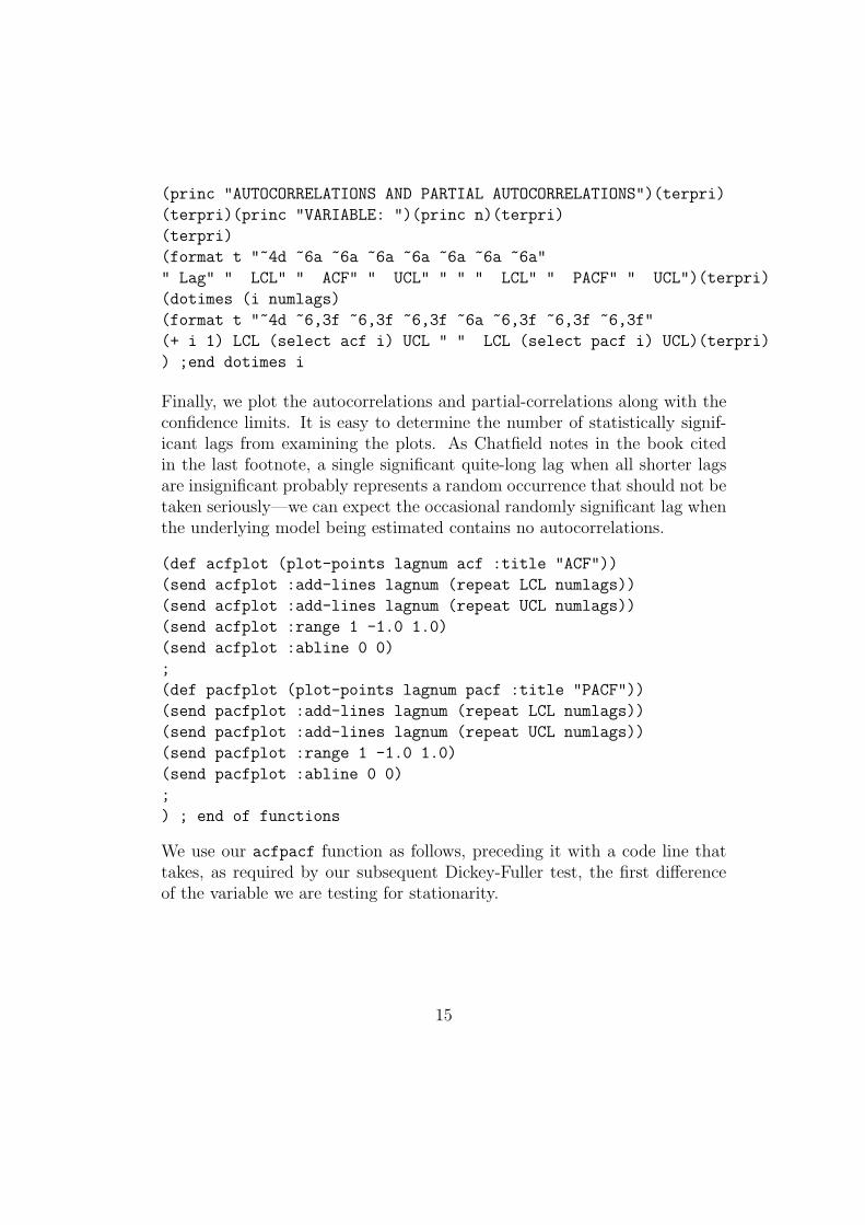
(princ "AUTOCORRELATIONS AND PARTIAL AUTOCORRELATIONS")(terpri)
(terpri)(princ "VARIABLE: ")(princ n)(terpri)
(terpri)
(format t "~4d ~6a ~6a ~6a ~6a ~6a ~6a ~6a"
" Lag" " LCL" " ACF" " UCL" " " " LCL" " PACF" " UCL")(terpri)
(dotimes (i numlags)
(format t "~4d ~6,3f ~6,3f ~6,3f ~6a ~6,3f ~6,3f ~6,3f"
(+ i 1) LCL (select acf i) UCL " " LCL (select pacf i) UCL)(terpri)
) ;end dotimes i
Finally, we plot the autocorrelations and partial-correlations along with theconfidence limits. It is easy to determine the number of statistically signif-icant lags from examining the plots. As Chatfield notes in the book citedin the last footnote, a single significant quite-long lag when all shorter lagsare insignificant probably represents a random occurrence that should not betaken seriously—we can expect the occasional randomly significant lag whenthe underlying model being estimated contains no autocorrelations.
(def acfplot (plot-points lagnum acf :title "ACF"))
(send acfplot :add-lines lagnum (repeat LCL numlags))
(send acfplot :add-lines lagnum (repeat UCL numlags))
(send acfplot :range 1 -1.0 1.0)
(send acfplot :abline 0 0)
;
(def pacfplot (plot-points lagnum pacf :title "PACF"))
(send pacfplot :add-lines lagnum (repeat LCL numlags))
(send pacfplot :add-lines lagnum (repeat UCL numlags))
(send pacfplot :range 1 -1.0 1.0)
(send pacfplot :abline 0 0)
;
) ; end of functions
We use our acfpacf function as follows, preceding it with a code line thattakes, as required by our subsequent Dickey-Fuller test, the first differenceof the variable we are testing for stationarity.
15

; XLISPSTAT BATCH FILE FOR UNIT ROOT TESTS
;
(load "ourfuncs")
(load "causqdat")
(variables)
;
; SET UP CANADA/U.S. REAL EXCHANGE RATE
;
(def rexcaus (remove-first 8 (* 100 (/ cpica (* exrcaus cpius)))))
;
(def plotrex (plot-lines (- dates74 1900) rexcaus
:title "Canada vs. U.S. Real Exchange Rate: Index -- 1974 = 100"))
;
(DFlags rexcaus 12)
;
(def drexcaus (- (remove-first 1 rexcaus)(remove-last 1 rexcaus)))
(acfpacf drexcaus "First Difference of Canada vs. U.S. Real Exchange Rate" 12)
The addition to our output as a result of these last two lines of code is
AUTOCORRELATIONS AND PARTIAL AUTOCORRELATIONS
VARIABLE: First Difference of Canadian vs. U.S. Real Exchange Rate
Lag LCL ACF UCL LCL PACF UCL
1 -0.165 0.338 0.165 -0.165 0.346 0.165
2 -0.165 0.012 0.165 -0.165 -0.127 0.165
3 -0.165 0.046 0.165 -0.165 0.106 0.165
4 -0.165 -0.092 0.165 -0.165 -0.174 0.165
5 -0.165 -0.097 0.165 -0.165 0.022 0.165
6 -0.165 0.064 0.165 -0.165 0.110 0.165
7 -0.165 0.134 0.165 -0.165 0.127 0.165
8 -0.165 0.051 0.165 -0.165 -0.053 0.165
9 -0.165 0.047 0.165 -0.165 -0.015 0.165
10 -0.165 0.002 0.165 -0.165 -0.061 0.165
11 -0.165 -0.013 0.165 -0.165 0.045 0.165
12 -0.165 0.004 0.165 -0.165 0.003 0.165
16

followed by the following two graphs.
17

It seems reasonable to go with the partial-autocorrelation function and setthe lag at three, which confirms the results suggested by our DFlags function.
We can now proceed to construct our dfunit function to do the Dickey-Fuller unit-root tests. The code lines are as follows with, as usual, my com-ments in between. Our function takes four arguments. The first, y, is theseries being examined and the second, n, is a text element denoting thename of that series. The third argument, l, is the number of lags and thefinal argument, s, is the the starting observation number, counting from 1.This latter argument allows us to start additional calculations at later dateswithout changing the number of lags.
(defun dfunit (y n l s)
"Args: (y n l s)
Performs an augmented Dickey-Fuller unit root text on the series y having
name n with l lags, starting at observation s (counting from 1)."
(terpri)
(princ "DICKEY-FULLER TEST --- ")(princ n)
(terpri)
(princ "Lags = ")
(princ l)
(terpri)
(princ "Starting observation = ")
(princ s)
(terpri)
(def lagy (remove-last 1 y))
(def newy (remove-first 1 y))
(def Dy (- newy lagy))
(def lagy (remove-first (- s 1) lagy))
(def newy (remove-first (- s 1) newy))
(def Dy (remove-first (- s l 1) Dy))
The first lines of code above print to screen the information about the test.Then we calculate the first difference of our variable and adjust both it andthe one-period lag of that variable to take into account the length of the lagchosen. Next, in the code below, we create the chosen number of lags of ∆yif the number of lags chosen is positive, calculate the number of observationsand print the corresponding information to the screen. We then constructthe trend variable and calculate the sum of squared deviations of ∆y fromits mean along with the sum of the squared values of that variable itself.
18

(if (> l 0)
(def Dymat (makelags l Dy)))
(def Dy (remove-first l Dy))
(def nobs (length Dy))
(princ "Number of observations = ")
(princ nobs)
(terpri)
(def trend (iseq 1 nobs))
(def SSDy (sum (^ (- Dy (mean Dy)) 2)))
(def DYSQ (sum (^ Dy 2)))
We then run the three regressions, using the if function to add the laggedvalues if one or more lags has been chosen and run the regression without lagsotherwise. Our first regression includes both a constant term (drift) and atrend. The second includes drift but no trend and the third includes neitherdrift (specified by the constant term) nor trend.
(if (> l 0)
(def dfreg1 (regression-model (list trend lagy Dymat) Dy :print nil))
(def dfreg1 (regression-model (list trend lagy) Dy :print nil))
) ; end if
(if (> l 0)
(def dfreg2 (regression-model (list lagy Dymat) Dy :print nil))
(def dfreg2 (regression-model (list lagy) Dy :print nil ))
) ; end if
(if (> l 0)
(def dfreg3 (regression-model (list lagy Dymat) Dy :intercept nil :print nil))
(def dfreg3 (regression-model (list lagy) Dy :intercept nil :print nil))
) ; end if
(if (> l 0) ; run regression with lags only
(def dfreg1r (regression-model (list Dymat) Dy :intercept nil :print nil))
) ; end if
(if (> l 0) ; run regression with constant and lags only
(def dfreg2r (regression-model (list Dymat) Dy :print nil))
) ; end if
Two restricted regressions are then added above, one with lags only and thesecond with a constant and lags only. Next we send the regression objectsmessages to retrieve the residual sums of squares, the coefficient estimates,
19

and the coefficient standard errors and construct the conventional t-statistics,the magnitudes of which will have to be compared with the critical valuesin the Dickey-Fuller tables. In addition we must keep in mind that thestandard error of a restricted regression with no lags, no trend and no laggedvalue of y is equal to the sum of the squared deviations of the dependentvariable from its mean, and that the standard error of a restricted regressioncontaining no variables is the sum of the squared values of the dependentvariable. Then we conduct F-tests of the null hypotheses that coefficientsof the trend and lagged value of y, and the coefficients of both the constantand trend and lagged value of y, are zero respectively in the first regressionand that the coefficients of the constant and lagged value of y are both zerothe second regression. A necessarily negative t-statistic for the coefficientof the lagged value of y in the third regression, which includes neither aconstant or tend, can be checked in the Dickey-Fuller table to determinewhether the null hypothesis of a zero coefficient of lagged y can be rejectedand the series is therefore stationary with no drift or trend. Thus, in the firsttwo regressions, we determine whether it is possible to establish stationaryaround trend and/or drift, keeping in mind that the trend variable reallymeasures the change in drift through time. Notice that the F-statistics arecalculated by taking the ratio of the increase in the standard error of theregression when variables are removed, divided by the number of variablesremoved, over the standard error of the unrestricted regression divided bythe degrees of freedom. And the F-statistic has as its two parameters thenumber of degrees of freedom in the numerator, represented by the numberof restrictions (or variables removed), and the number of degrees of freedomin the unrestricted regression in the denominator.
(def SSE1 (send dfreg1 :residual-sum-of-squares))
(def SSE1 (send dfreg1 :residual-sum-of-squares))
(def df1 (send dfreg1 :df))
(def SSE2 (send dfreg2 :residual-sum-of-squares))
(def df2 (send dfreg2 :df))
(def SSE3 (send dfreg3 :residual-sum-of-squares))
(def df3 (send dfreg3 :df))
(def coefs1 (send dfreg1 :coef-estimates))
(def trat1 (/ (send dfreg1 :coef-estimates)(send dfreg1
:coef-standard-errors)))
(def coefs2 (send dfreg2 :coef-estimates))
20
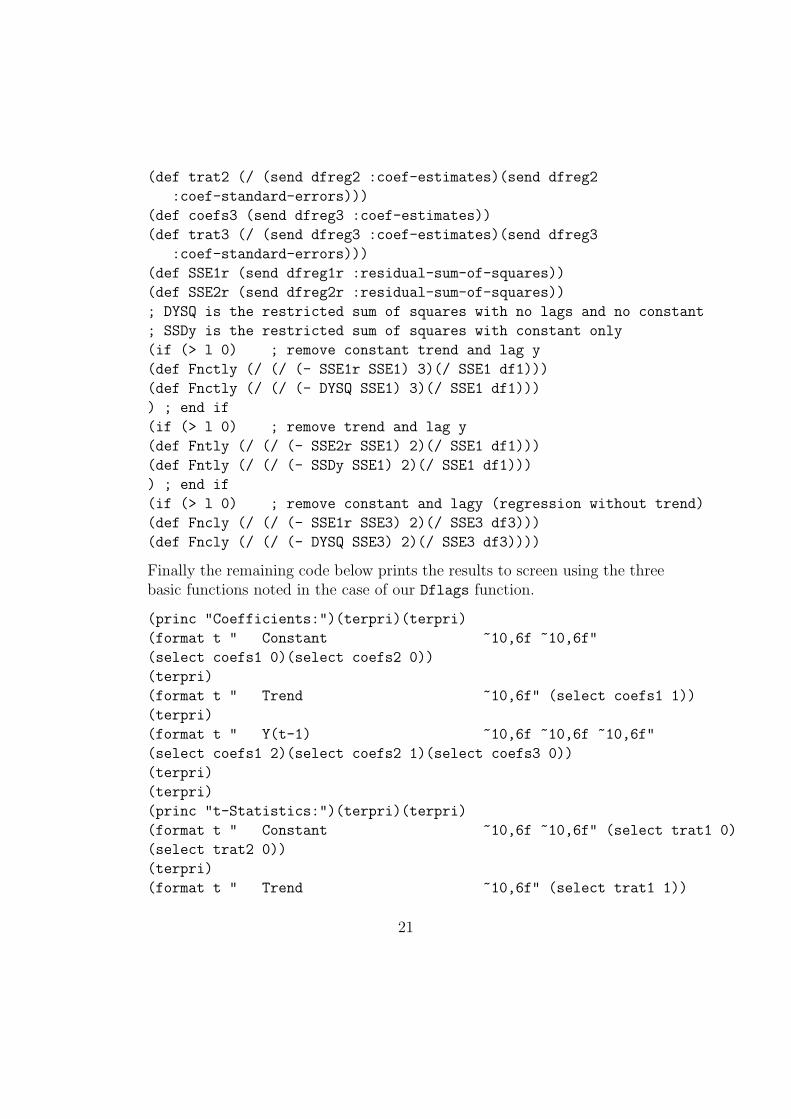
(def trat2 (/ (send dfreg2 :coef-estimates)(send dfreg2
:coef-standard-errors)))
(def coefs3 (send dfreg3 :coef-estimates))
(def trat3 (/ (send dfreg3 :coef-estimates)(send dfreg3
:coef-standard-errors)))
(def SSE1r (send dfreg1r :residual-sum-of-squares))
(def SSE2r (send dfreg2r :residual-sum-of-squares))
; DYSQ is the restricted sum of squares with no lags and no constant
; SSDy is the restricted sum of squares with constant only
(if (> l 0) ; remove constant trend and lag y
(def Fnctly (/ (/ (- SSE1r SSE1) 3)(/ SSE1 df1)))
(def Fnctly (/ (/ (- DYSQ SSE1) 3)(/ SSE1 df1)))
) ; end if
(if (> l 0) ; remove trend and lag y
(def Fntly (/ (/ (- SSE2r SSE1) 2)(/ SSE1 df1)))
(def Fntly (/ (/ (- SSDy SSE1) 2)(/ SSE1 df1)))
) ; end if
(if (> l 0) ; remove constant and lagy (regression without trend)
(def Fncly (/ (/ (- SSE1r SSE3) 2)(/ SSE3 df3)))
(def Fncly (/ (/ (- DYSQ SSE3) 2)(/ SSE3 df3))))
Finally the remaining code below prints the results to screen using the threebasic functions noted in the case of our Dflags function.
(princ "Coefficients:")(terpri)(terpri)
(format t " Constant ~10,6f ~10,6f"
(select coefs1 0)(select coefs2 0))
(terpri)
(format t " Trend ~10,6f" (select coefs1 1))
(terpri)
(format t " Y(t-1) ~10,6f ~10,6f ~10,6f"
(select coefs1 2)(select coefs2 1)(select coefs3 0))
(terpri)
(terpri)
(princ "t-Statistics:")(terpri)(terpri)
(format t " Constant ~10,6f ~10,6f" (select trat1 0)
(select trat2 0))
(terpri)
(format t " Trend ~10,6f" (select trat1 1))
21
(terpri)
(format t " Y(t-1) ~10,6f ~10,6f ~10,6f"
(select trat1 2)(select trat2 1)(select trat3 0))
(terpri)
(if (> l 0)
(format t " Lagged (Y(t)-Y(t-1)) ~10,6f ~10,6f ~10,6f"
(select trat1 3)(select trat2 2)(select trat3 1)))
(terpri)
(if (> l 1)
(dotimes (i (- l 1))
(format t " ........ ~10,6f ~10,6f ~10,6f"
(select trat1 (+ i 4))(select trat2 (+ i 3))(select trat3 (+ i 2)))
(terpri)))
(terpri)
(princ "F-Statistics:")(terpri)(terpri)
(format t " All Three Coefficients = 0 ~10,6f" Fnctly)
(terpri)
(format t " Constant & Y(t-1) Coef = 0 ~20,6f" Fntly)
(terpri)
(format t " Trend & Y(t-1) Coefs = 0 ~10,6f" Fncly)
(terpri)
(terpri)
) ;end function
We can now apply our dfunit function by adding the following line of codeto our batch file,
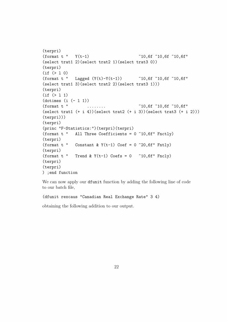
(dfunit rexcaus "Canadian Real Exchange Rate" 3 4)
obtaining the following addition to our output.
22

DICKEY-FULLER TEST --- Canadian Real Exchange Rate
Lags = 3
Starting observation = 4
Number of observations = 144
Coefficients:
Constant 1.917298 2.773078
Trend 0.003669
Y(t-1) -0.026069 -0.033138 -0.000283
t-Statistics:
Constant 1.029580 1.841325
Trend 0.783369
Y(t-1) -1.295709 -1.845327 -0.138492
Lagged (Y(t)-Y(t-1)) 4.785584 4.965487 4.832090
........ -1.798384 -1.721166 -1.869615
........ 1.314176 1.479683 1.241849
F-Statistics:
All Three Coefficients = 0 1.338059
Trend & Y(t-1) Coefs = 0 2.004717
Constant & Y(t-1) Coefs = 0 1.704993
The t-ratios above are clearly smaller than would be necessary for us to rejectnull hypotheses using the confidence limits in the Dickey-Fuller table. It isalso obvious that the F-statistics are far too low to enable us to reject thenull hypotheses in question.
23

The Dickey-Fuller tests assume that the shocks ϵt are statistically inde-pendent of each other and have a constant variance. An alternative proce-dure, developed by Peter Phillips and Pierre Perron, can be used to conductthe tests under the assumption that there is some interdependence of theshocks and they are heterogeneously distributed. Theirs is a modified ver-sion of the Dickey-Fuller approach that incorporates adjustments for serialcorrelation and heteroskedasticity of the sort involved in HAC adjustmentsto coefficient-standard-errors. It turns out, however, that the probability ofdistortions in these estimates in finite samples makes them a bit controver-sial and has prompted continuing extensions of the process through whichthey are calculated. Accordingly, given the complexity of figuring out andprogramming the optimal formulation of the test, we will here focus entirelyon Dickey-Fuller tests, as consistent with the modern applied econometricsliterature.10
Suppose, alternatively, that we want to run the Dickey-Fullertest in Gretl. The simplest way to do this is to fire-up Gretl and load thedata file causdata.gdt. If no real exchange rate series is present in the file,we simply click on add and scroll down to Define new variable and typethe following code in the window that appears:
REXCAUS = 100*CPICA/(EXRCAUS*CPIUS
Then click on variable and scroll down to and click on Augmented Dickey-Fuller
test (the word augmented refers to the option of including lags of ∆y ). Awindow will appear in which we give Gretl the appropriate instructions. Weshould highlight the following options
test without constant
test with constant
test with constant and trend
test down from maximum lag order
use level of variable
and then, acting as if we did not know how many lags to use, set the lag-order at 12, the maximum number we chose when working with XLispStat.Upon clicking on the OK button we obtain the following results in a separatewindow.
10For example, Russell Davidson and James G. MacKinnon in their peviously citedgraduate-level textbook, do not include the Phillips-Perron test for reasons stated on page623.
24
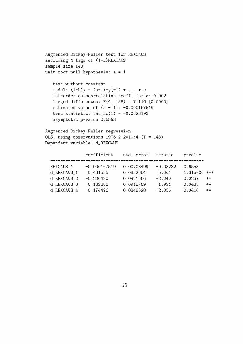
Augmented Dickey-Fuller test for REXCAUS
including 4 lags of (1-L)REXCAUS
sample size 143
unit-root null hypothesis: a = 1
test without constant
model: (1-L)y = (a-1)*y(-1) + ... + e
1st-order autocorrelation coeff. for e: 0.002
lagged differences: F(4, 138) = 7.116 [0.0000]
estimated value of (a - 1): -0.000167519
test statistic: tau_nc(1) = -0.0823193
asymptotic p-value 0.6553
Augmented Dickey-Fuller regression
OLS, using observations 1975:2-2010:4 (T = 143)
Dependent variable: d_REXCAUS
coefficient std. error t-ratio p-value
-------------------------------------------------------------
REXCAUS_1 -0.000167519 0.00203499 -0.08232 0.6553
d_REXCAUS_1 0.431535 0.0852664 5.061 1.31e-06 ***
d_REXCAUS_2 -0.206480 0.0921666 -2.240 0.0267 **
d_REXCAUS_3 0.182883 0.0918769 1.991 0.0485 **
d_REXCAUS_4 -0.174496 0.0848528 -2.056 0.0416 **
25
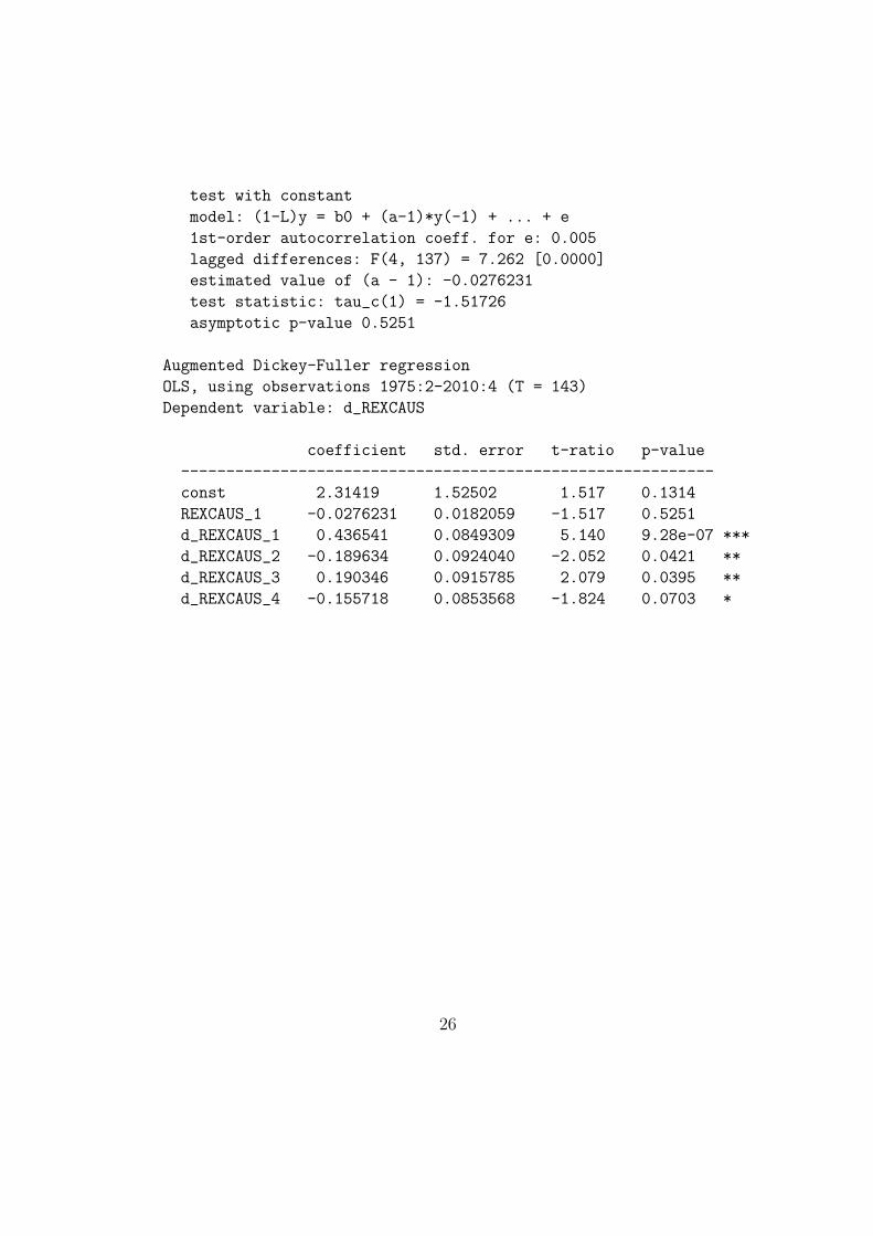
test with constant
model: (1-L)y = b0 + (a-1)*y(-1) + ... + e
1st-order autocorrelation coeff. for e: 0.005
lagged differences: F(4, 137) = 7.262 [0.0000]
estimated value of (a - 1): -0.0276231
test statistic: tau_c(1) = -1.51726
asymptotic p-value 0.5251
Augmented Dickey-Fuller regression
OLS, using observations 1975:2-2010:4 (T = 143)
Dependent variable: d_REXCAUS
coefficient std. error t-ratio p-value
-----------------------------------------------------------
const 2.31419 1.52502 1.517 0.1314
REXCAUS_1 -0.0276231 0.0182059 -1.517 0.5251
d_REXCAUS_1 0.436541 0.0849309 5.140 9.28e-07 ***
d_REXCAUS_2 -0.189634 0.0924040 -2.052 0.0421 **
d_REXCAUS_3 0.190346 0.0915785 2.079 0.0395 **
d_REXCAUS_4 -0.155718 0.0853568 -1.824 0.0703 *
26
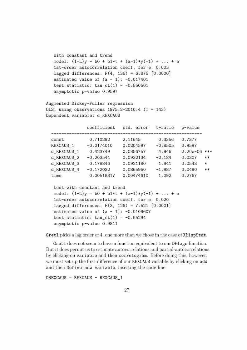
with constant and trend
model: (1-L)y = b0 + b1*t + (a-1)*y(-1) + ... + e
1st-order autocorrelation coeff. for e: 0.003
lagged differences: F(4, 136) = 6.875 [0.0000]
estimated value of (a - 1): -0.017401
test statistic: tau_ct(1) = -0.850501
asymptotic p-value 0.9597
Augmented Dickey-Fuller regression
OLS, using observations 1975:2-2010:4 (T = 143)
Dependent variable: d_REXCAUS
coefficient std. error t-ratio p-value
-----------------------------------------------------------
const 0.710292 2.11645 0.3356 0.7377
REXCAUS_1 -0.0174010 0.0204597 -0.8505 0.9597
d_REXCAUS_1 0.423749 0.0856757 4.946 2.20e-06 ***
d_REXCAUS_2 -0.203544 0.0932134 -2.184 0.0307 **
d_REXCAUS_3 0.178846 0.0921180 1.941 0.0543 *
d_REXCAUS_4 -0.172032 0.0865950 -1.987 0.0490 **
time 0.00518317 0.00474610 1.092 0.2767
test with constant and trend
model: (1-L)y = b0 + b1*t + (a-1)*y(-1) + ... + e
1st-order autocorrelation coeff. for e: 0.020
lagged differences: F(3, 126) = 7.521 [0.0001]
estimated value of (a - 1): -0.0109607
test statistic: tau_ct(1) = -0.55294
asymptotic p-value 0.9811
Gretl picks a lag order of 4, one more than we chose in the case of XLispStat.
Gretl does not seem to have a function equivalent to our DFlags function.But it does permit us to estimate autocorrelations and partial-autocorrelationsby clicking on variable and then correlogram. Before doing this, however,we must set up the first-difference of our REXCAUS variable by clicking on add
and then Define new variable, inserting the code line
DREXCAUS = REXCAUS - REXCAUS_1
27
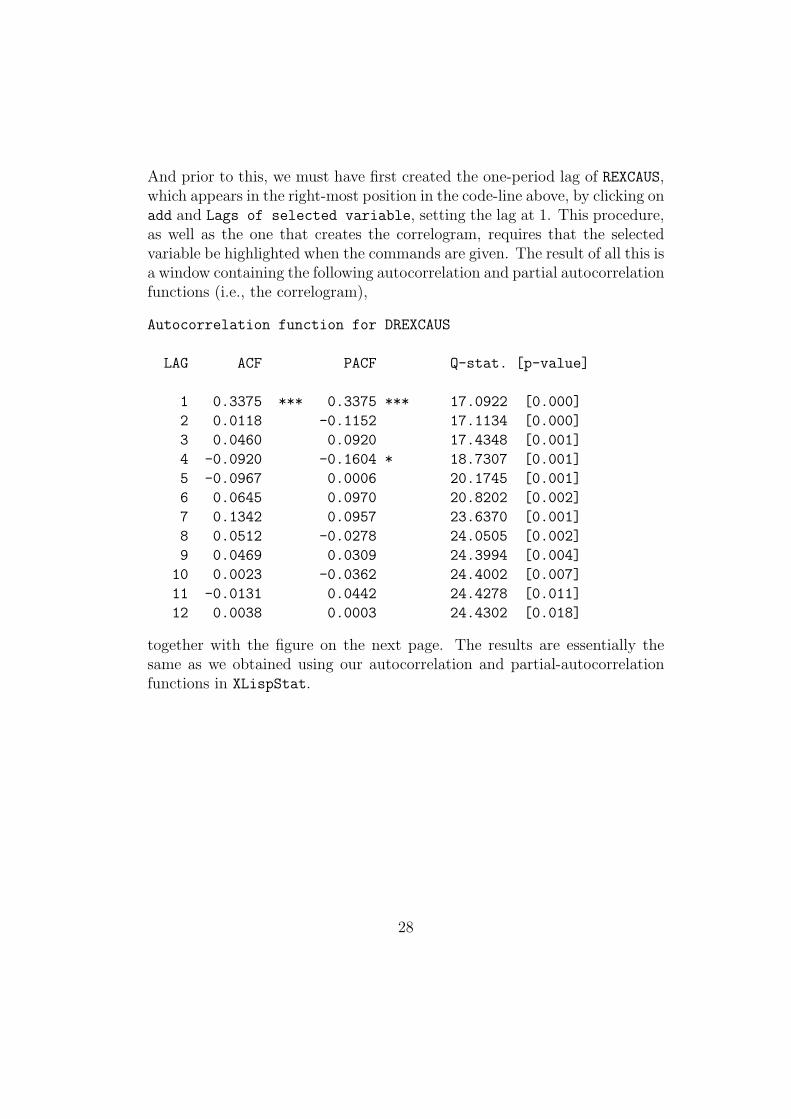
And prior to this, we must have first created the one-period lag of REXCAUS,which appears in the right-most position in the code-line above, by clicking onadd and Lags of selected variable, setting the lag at 1. This procedure,as well as the one that creates the correlogram, requires that the selectedvariable be highlighted when the commands are given. The result of all this isa window containing the following autocorrelation and partial autocorrelationfunctions (i.e., the correlogram),
Autocorrelation function for DREXCAUS
LAG ACF PACF Q-stat. [p-value]
1 0.3375 *** 0.3375 *** 17.0922 [0.000]
2 0.0118 -0.1152 17.1134 [0.000]
3 0.0460 0.0920 17.4348 [0.001]
4 -0.0920 -0.1604 * 18.7307 [0.001]
5 -0.0967 0.0006 20.1745 [0.001]
6 0.0645 0.0970 20.8202 [0.002]
7 0.1342 0.0957 23.6370 [0.001]
8 0.0512 -0.0278 24.0505 [0.002]
9 0.0469 0.0309 24.3994 [0.004]
10 0.0023 -0.0362 24.4002 [0.007]
11 -0.0131 0.0442 24.4278 [0.011]
12 0.0038 0.0003 24.4302 [0.018]
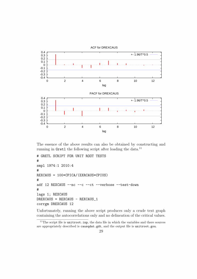
together with the figure on the next page. The results are essentially thesame as we obtained using our autocorrelation and partial-autocorrelationfunctions in XLispStat.
28
-0.4-0.3-0.2-0.1
0 0.1 0.2 0.3 0.4
0 2 4 6 8 10 12
lag
ACF for DREXCAUS
+- 1.96/T^0.5
-0.4-0.3-0.2-0.1
0 0.1 0.2 0.3 0.4
0 2 4 6 8 10 12
lag
PACF for DREXCAUS
+- 1.96/T^0.5
The essence of the above results can also be obtained by constructing andrunning in Gretl the following script after loading the data.11
# GRETL SCRIPT FOR UNIT ROOT TESTS
#
smpl 1974:1 2010:4
#
REXCAUS = 100*CPICA/(EXRCAUS*CPIUS)
#
adf 12 REXCAUS --nc --c --ct --verbose --test-down
#
lags 1; REXCAUS
DREXCAUS = REXCAUS - REXCAUS_1
corrgm DREXCAUS 12
Unfortunately, running the above script produces only a crude text graphcontaining the autocorrelations only and no delineation of the critical values.
11The script file is unitroot.inp, the data file in which the variables and there sourcesare appropriately described is causqdat.gdt, and the output file is unitroot.gou.
29
It is necessary to highlight the variable DREXCAUS and then click on variable
and then correlogram to get the pretty graph above containing both the au-tocorrelations and partial-autocorrelations with the 5% critical values high-lighted. The Q-statistics in the results above test whether the current andprevious autocorrelations are zero—if that statistic is larger than some crit-ical value we can reject the null hypothesis of no significant autocorrelation.The P-Values above clearly indicate that the series is not white-noise.
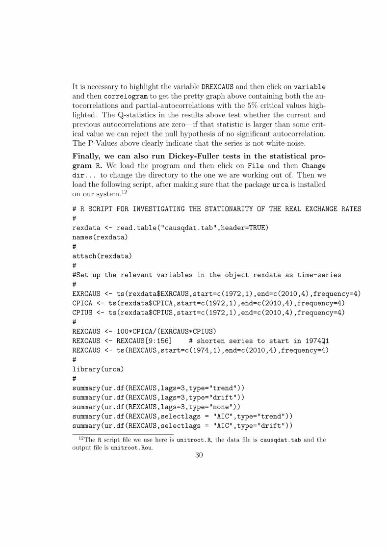
Finally, we can also run Dickey-Fuller tests in the statistical pro-gram R. We load the program and then click on File and then Change
dir... to change the directory to the one we are working out of. Then weload the following script, after making sure that the package urca is installedon our system.12
# R SCRIPT FOR INVESTIGATING THE STATIONARITY OF THE REAL EXCHANGE RATES
#
rexdata <- read.table("causqdat.tab",header=TRUE)
names(rexdata)
#
attach(rexdata)
#
#Set up the relevant variables in the object rexdata as time-series
#
EXRCAUS <- ts(rexdata$EXRCAUS,start=c(1972,1),end=c(2010,4),frequency=4)
CPICA <- ts(rexdata$CPICA,start=c(1972,1),end=c(2010,4),frequency=4)
CPIUS <- ts(rexdata$CPIUS,start=c(1972,1),end=c(2010,4),frequency=4)
#
REXCAUS <- 100*CPICA/(EXRCAUS*CPIUS)
REXCAUS <- REXCAUS[9:156] # shorten series to start in 1974Q1
REXCAUS <- ts(REXCAUS,start=c(1974,1),end=c(2010,4),frequency=4)
#
library(urca)
#
summary(ur.df(REXCAUS,lags=3,type="trend"))
summary(ur.df(REXCAUS,lags=3,type="drift"))
summary(ur.df(REXCAUS,lags=3,type="none"))
summary(ur.df(REXCAUS,selectlags = "AIC",type="trend"))
summary(ur.df(REXCAUS,selectlags = "AIC",type="drift"))
12The R script file we use here is unitroot.R, the data file is causqdat.tab and theoutput file is unitroot.Rou.
30
summary(ur.df(REXCAUS,selectlags = "AIC",type="none"))
We perform the Dickey-Fuller tests using the ur.df function in two ways—once with our previously chosen lag of 3 and once letting R choose the optimallag using the AIC. We obtain the following results.
R version 2.10.1 (2009-12-14)
Copyright (C) 2009 The R Foundation for Statistical Computing
ISBN 3-900051-07-0
R is free software and comes with ABSOLUTELY NO WARRANTY.
You are welcome to redistribute it under certain conditions.
Type ’license()’ or ’licence()’ for distribution details.
Natural language support but running in an English locale
R is a collaborative project with many contributors.
Type ’contributors()’ for more information and
’citation()’ on how to cite R or R packages in publications.
Type ’demo()’ for some demos, ’help()’ for on-line help, or
’help.start()’ for an HTML browser interface to help.
Type ’q()’ to quit R.
> # R SCRIPT FOR INVESTIGATING THE STATIONARITY OF THE REAL EXCHANGE RATES
> #
> rexdata <- read.table("causqdat.tab",header=TRUE)
> names(rexdata)
[1] "X.YEAR" "IPDCA" "IPDUS" "EXRCAUS" "GDPCA" "GDPUS" "EXPGSUS"
[8] "IMPGSUS" "EXPGSCA" "IMPGSCA" "CPICA" "PEXPUS" "PIMPUS" "CPIUS"
[15] "PCOMM" "PCOMXEN" "PENERGY" "PCROIL" "M1CA" "M2CA" "M1US"
[22] "M2US"
> #
> #Set up the relevant variables in the object rexdata as time-series
> #
> EXRCAUS <- ts(rexdata$EXRCAUS,start=c(1972,1),end=c(2010,4),frequency=4)
> CPICA <- ts(rexdata$CPICA,start=c(1972,1),end=c(2010,4),frequency=4)
> CPIUS <- ts(rexdata$CPIUS,start=c(1972,1),end=c(2010,4),frequency=4)
> #
31

> REXCAUS <- 100*CPICA/(EXRCAUS*CPIUS)
> REXCAUS <- REXCAUS[9:156] # shorten series to start in 1974Q1
> REXCAUS <- ts(REXCAUS,start=c(1974,1),end=c(2010,4),frequency=4)
> #
> library(urca)
> #
32

> summary(ur.df(REXCAUS,lags=3,type="trend"))
>
###############################################
# Augmented Dickey-Fuller Test Unit Root Test #
###############################################
Test regression trend
Call:
lm(formula = z.diff ~ z.lag.1 + 1 + tt + z.diff.lag)
Residuals:
Min 1Q Median 3Q Max
-10.4288 -1.0699 -0.1282 1.0384 5.9248
Coefficients:
Estimate Std. Error t value Pr(>|t|)
(Intercept) 1.906292 1.870491 1.019 0.3099
z.lag.1 -0.026069 0.020120 -1.296 0.1972
tt 0.003669 0.004683 0.783 0.4348
z.diff.lag1 0.411959 0.086083 4.786 4.33e-06 ***
z.diff.lag2 -0.164778 0.091625 -1.798 0.0743 .
z.diff.lag3 0.113852 0.086634 1.314 0.1910
---
Signif. codes: 0 *** 0.001 ** 0.01 * 0.05 . 0.1 1
Residual standard error: 2.041 on 138 degrees of freedom
Multiple R-squared: 0.169, Adjusted R-squared: 0.1389
F-statistic: 5.614 on 5 and 138 DF, p-value: 9.658e-05
Value of test-statistic is: -1.2957 1.3381 2.0047
Critical values for test statistics:
1pct 5pct 10pct
tau3 -3.99 -3.43 -3.13
phi2 6.22 4.75 4.07
33
phi3 8.43 6.49 5.47
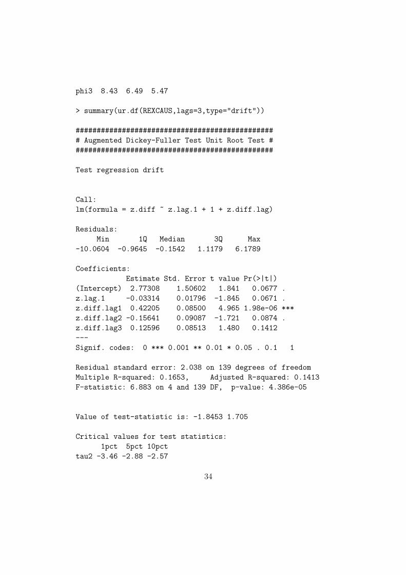
> summary(ur.df(REXCAUS,lags=3,type="drift"))
###############################################
# Augmented Dickey-Fuller Test Unit Root Test #
###############################################
Test regression drift
Call:
lm(formula = z.diff ~ z.lag.1 + 1 + z.diff.lag)
Residuals:
Min 1Q Median 3Q Max
-10.0604 -0.9645 -0.1542 1.1179 6.1789
Coefficients:
Estimate Std. Error t value Pr(>|t|)
(Intercept) 2.77308 1.50602 1.841 0.0677 .
z.lag.1 -0.03314 0.01796 -1.845 0.0671 .
z.diff.lag1 0.42205 0.08500 4.965 1.98e-06 ***
z.diff.lag2 -0.15641 0.09087 -1.721 0.0874 .
z.diff.lag3 0.12596 0.08513 1.480 0.1412
---
Signif. codes: 0 *** 0.001 ** 0.01 * 0.05 . 0.1 1
Residual standard error: 2.038 on 139 degrees of freedom
Multiple R-squared: 0.1653, Adjusted R-squared: 0.1413
F-statistic: 6.883 on 4 and 139 DF, p-value: 4.386e-05
Value of test-statistic is: -1.8453 1.705
Critical values for test statistics:
1pct 5pct 10pct
tau2 -3.46 -2.88 -2.57
34
phi1 6.52 4.63 3.81
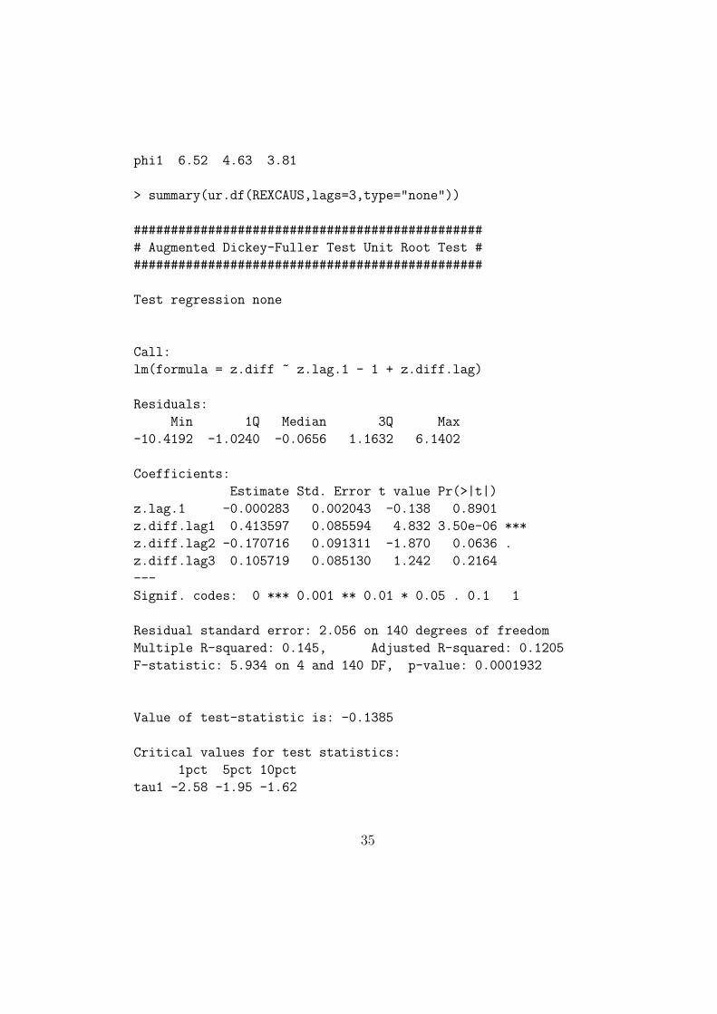
> summary(ur.df(REXCAUS,lags=3,type="none"))
###############################################
# Augmented Dickey-Fuller Test Unit Root Test #
###############################################
Test regression none
Call:
lm(formula = z.diff ~ z.lag.1 - 1 + z.diff.lag)
Residuals:
Min 1Q Median 3Q Max
-10.4192 -1.0240 -0.0656 1.1632 6.1402
Coefficients:
Estimate Std. Error t value Pr(>|t|)
z.lag.1 -0.000283 0.002043 -0.138 0.8901
z.diff.lag1 0.413597 0.085594 4.832 3.50e-06 ***
z.diff.lag2 -0.170716 0.091311 -1.870 0.0636 .
z.diff.lag3 0.105719 0.085130 1.242 0.2164
---
Signif. codes: 0 *** 0.001 ** 0.01 * 0.05 . 0.1 1
Residual standard error: 2.056 on 140 degrees of freedom
Multiple R-squared: 0.145, Adjusted R-squared: 0.1205
F-statistic: 5.934 on 4 and 140 DF, p-value: 0.0001932
Value of test-statistic is: -0.1385
Critical values for test statistics:
1pct 5pct 10pct
tau1 -2.58 -1.95 -1.62
35

> summary(ur.df(REXCAUS,selectlags = "AIC",type="trend"))
###############################################
# Augmented Dickey-Fuller Test Unit Root Test #
###############################################
Test regression trend
Call:
lm(formula = z.diff ~ z.lag.1 + 1 + tt + z.diff.lag)
Residuals:
Min 1Q Median 3Q Max
-10.8480 -1.0609 -0.1068 0.9765 6.0598
Coefficients:
Estimate Std. Error t value Pr(>|t|)
(Intercept) 2.019015 1.781982 1.133 0.259
z.lag.1 -0.027608 0.019209 -1.437 0.153
tt 0.003788 0.004489 0.844 0.400
z.diff.lag 0.347649 0.080237 4.333 2.77e-05 ***
---
Signif. codes: 0 *** 0.001 ** 0.01 * 0.05 . 0.1 1
Residual standard error: 2.045 on 142 degrees of freedom
Multiple R-squared: 0.1457, Adjusted R-squared: 0.1277
F-statistic: 8.074 on 3 and 142 DF, p-value: 5.279e-05
Value of test-statistic is: -1.4372 1.5601 2.3399
Critical values for test statistics:
1pct 5pct 10pct
tau3 -3.99 -3.43 -3.13
phi2 6.22 4.75 4.07
phi3 8.43 6.49 5.47
36

> summary(ur.df(REXCAUS,selectlags = "AIC",type="drift"))
###############################################
# Augmented Dickey-Fuller Test Unit Root Test #
###############################################
Test regression drift
Call:
lm(formula = z.diff ~ z.lag.1 + 1 + z.diff.lag)
Residuals:
Min 1Q Median 3Q Max
-10.5012 -1.0426 -0.1600 1.0615 6.3060
Coefficients:
Estimate Std. Error t value Pr(>|t|)
(Intercept) 2.88233 1.45751 1.978 0.0499 *
z.lag.1 -0.03456 0.01733 -1.994 0.0481 *
z.diff.lag 0.36086 0.07862 4.590 9.61e-06 ***
---
Signif. codes: 0 *** 0.001 ** 0.01 * 0.05 . 0.1 1
Residual standard error: 2.043 on 143 degrees of freedom
Multiple R-squared: 0.1414, Adjusted R-squared: 0.1294
F-statistic: 11.78 on 2 and 143 DF, p-value: 1.84e-05
Value of test-statistic is: -1.9939 1.9882
Critical values for test statistics:
1pct 5pct 10pct
tau2 -3.46 -2.88 -2.57
phi1 6.52 4.63 3.81
37

> summary(ur.df(REXCAUS,selectlags = "AIC",type="none"))
###############################################
# Augmented Dickey-Fuller Test Unit Root Test #
###############################################
Test regression none
Call:
lm(formula = z.diff ~ z.lag.1 - 1 + z.diff.lag)
Residuals:
Min 1Q Median 3Q Max
-10.8114 -1.0104 -0.1352 1.0519 6.4942
Coefficients:
Estimate Std. Error t value Pr(>|t|)
z.lag.1 -0.0005153 0.0020310 -0.254 0.8
z.diff.lag 0.3463609 0.0790608 4.381 2.26e-05 ***
---
Signif. codes: 0 *** 0.001 ** 0.01 * 0.05 . 0.1 1
Residual standard error: 2.063 on 144 degrees of freedom
Multiple R-squared: 0.118, Adjusted R-squared: 0.1057
F-statistic: 9.632 on 2 and 144 DF, p-value: 0.0001186
Value of test-statistic is: -0.2537
Critical values for test statistics:
1pct 5pct 10pct
tau1 -2.58 -1.95 -1.62
38
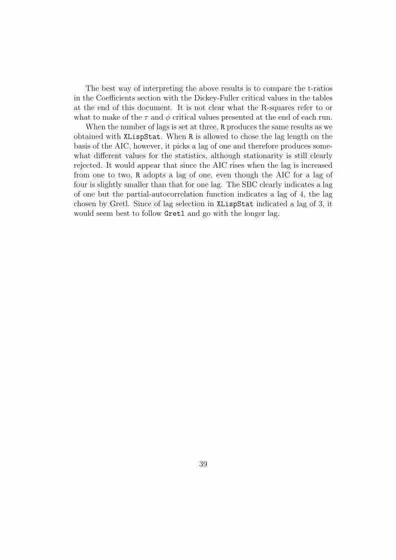
The best way of interpreting the above results is to compare the t-ratiosin the Coefficients section with the Dickey-Fuller critical values in the tablesat the end of this document. It is not clear what the R-squares refer to orwhat to make of the τ and ϕ critical values presented at the end of each run.
When the number of lags is set at three, R produces the same results as weobtained with XLispStat. When R is allowed to chose the lag length on thebasis of the AIC, however, it picks a lag of one and therefore produces some-what different values for the statistics, although stationarity is still clearlyrejected. It would appear that since the AIC rises when the lag is increasedfrom one to two, R adopts a lag of one, even though the AIC for a lag offour is slightly smaller than that for one lag. The SBC clearly indicates a lagof one but the partial-autocorrelation function indicates a lag of 4, the lagchosen by Gretl. Since of lag selection in XLispStat indicated a lag of 3, itwould seem best to follow Gretl and go with the longer lag.
39
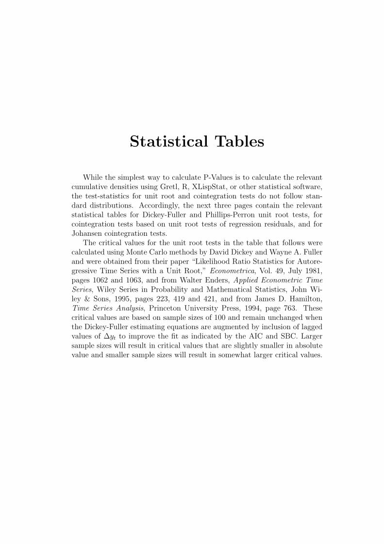
Statistical Tables
While the simplest way to calculate P-Values is to calculate the relevantcumulative densities using Gretl, R, XLispStat, or other statistical software,the test-statistics for unit root and cointegration tests do not follow stan-dard distributions. Accordingly, the next three pages contain the relevantstatistical tables for Dickey-Fuller and Phillips-Perron unit root tests, forcointegration tests based on unit root tests of regression residuals, and forJohansen cointegration tests.
The critical values for the unit root tests in the table that follows werecalculated using Monte Carlo methods by David Dickey and Wayne A. Fullerand were obtained from their paper “Likelihood Ratio Statistics for Autore-gressive Time Series with a Unit Root,” Econometrica, Vol. 49, July 1981,pages 1062 and 1063, and from Walter Enders, Applied Econometric TimeSeries, Wiley Series in Probability and Mathematical Statistics, John Wi-ley & Sons, 1995, pages 223, 419 and 421, and from James D. Hamilton,Time Series Analysis, Princeton University Press, 1994, page 763. Thesecritical values are based on sample sizes of 100 and remain unchanged whenthe Dickey-Fuller estimating equations are augmented by inclusion of laggedvalues of ∆yt to improve the fit as indicated by the AIC and SBC. Largersample sizes will result in critical values that are slightly smaller in absolutevalue and smaller sample sizes will result in somewhat larger critical values.
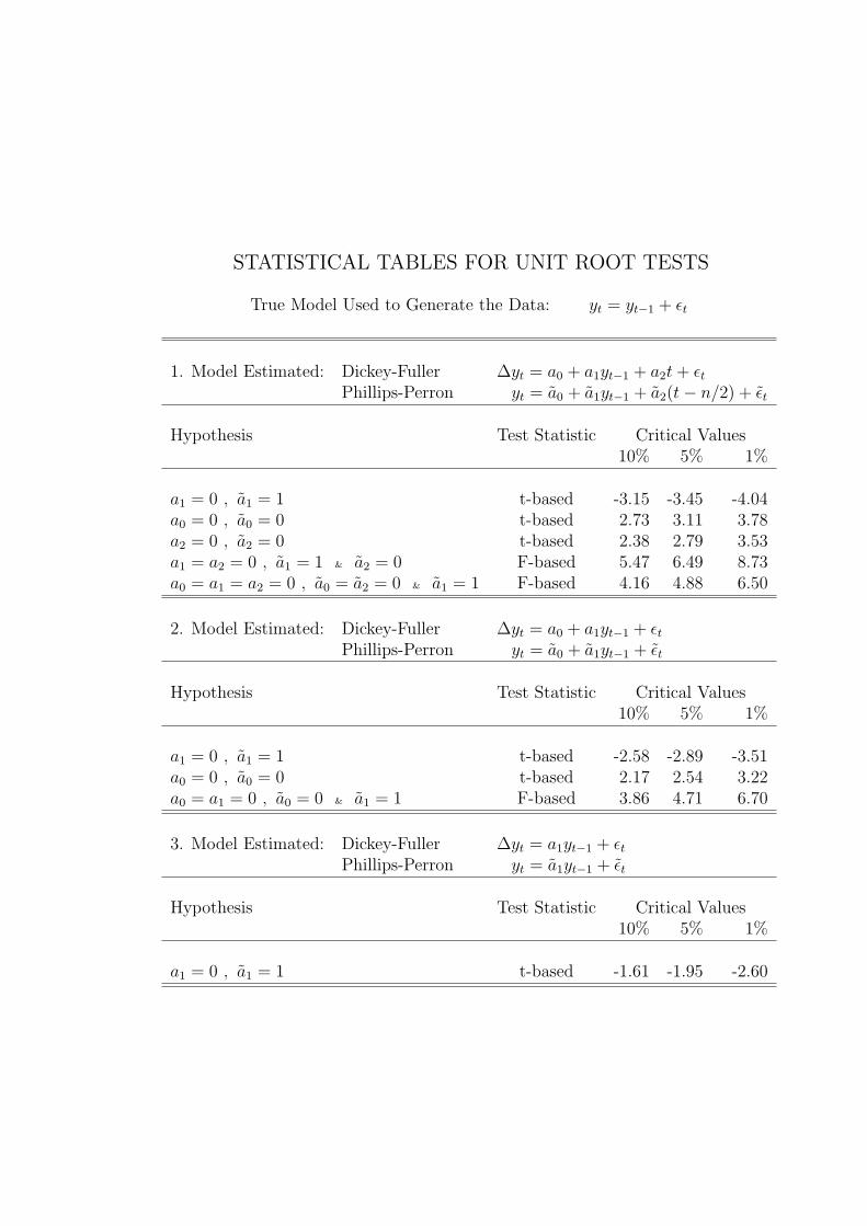
STATISTICAL TABLES FOR UNIT ROOT TESTS
True Model Used to Generate the Data: yt = yt−1 + ϵt
1. Model Estimated: Dickey-Fuller ∆yt = a0 + a1yt−1 + a2t+ ϵtPhillips-Perron yt = a0 + a1yt−1 + a2(t− n/2) + ϵt
Hypothesis Test Statistic Critical Values10% 5% 1%
a1 = 0 , a1 = 1 t-based -3.15 -3.45 -4.04a0 = 0 , a0 = 0 t-based 2.73 3.11 3.78a2 = 0 , a2 = 0 t-based 2.38 2.79 3.53a1 = a2 = 0 , a1 = 1 & a2 = 0 F-based 5.47 6.49 8.73a0 = a1 = a2 = 0 , a0 = a2 = 0 & a1 = 1 F-based 4.16 4.88 6.50
2. Model Estimated: Dickey-Fuller ∆yt = a0 + a1yt−1 + ϵtPhillips-Perron yt = a0 + a1yt−1 + ϵt
Hypothesis Test Statistic Critical Values10% 5% 1%
a1 = 0 , a1 = 1 t-based -2.58 -2.89 -3.51a0 = 0 , a0 = 0 t-based 2.17 2.54 3.22a0 = a1 = 0 , a0 = 0 & a1 = 1 F-based 3.86 4.71 6.70
3. Model Estimated: Dickey-Fuller ∆yt = a1yt−1 + ϵtPhillips-Perron yt = a1yt−1 + ϵt
Hypothesis Test Statistic Critical Values10% 5% 1%
a1 = 0 , a1 = 1 t-based -1.61 -1.95 -2.60
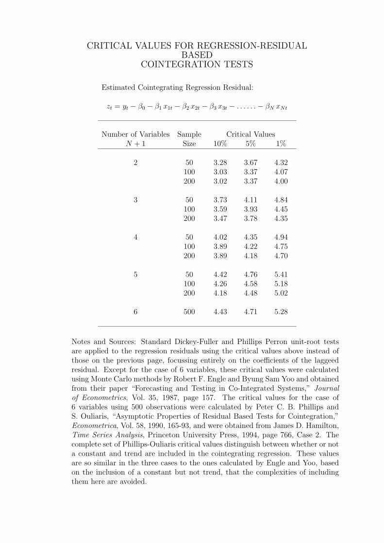
CRITICAL VALUES FOR REGRESSION-RESIDUALBASED
COINTEGRATION TESTS
Estimated Cointegrating Regression Residual:
zt = yt − β0 − β1 x1t − β2 x2t − β3 x3t − . . . . . .− βN xNt
Number of Variables Sample Critical ValuesN + 1 Size 10% 5% 1%
2 50 3.28 3.67 4.32100 3.03 3.37 4.07200 3.02 3.37 4.00
3 50 3.73 4.11 4.84100 3.59 3.93 4.45200 3.47 3.78 4.35
4 50 4.02 4.35 4.94100 3.89 4.22 4.75200 3.89 4.18 4.70
5 50 4.42 4.76 5.41100 4.26 4.58 5.18200 4.18 4.48 5.02
6 500 4.43 4.71 5.28
Notes and Sources: Standard Dickey-Fuller and Phillips Perron unit-root testsare applied to the regression residuals using the critical values above instead ofthose on the previous page, focussing entirely on the coefficients of the laggeedresidual. Except for the case of 6 variables, these critical values were calculatedusing Monte Carlo methods by Robert F. Engle and Byung Sam Yoo and obtainedfrom their paper “Forecasting and Testing in Co-Integrated Systems,” Journalof Econometrics, Vol. 35, 1987, page 157. The critical values for the case of6 variables using 500 observations were calculated by Peter C. B. Phillips andS. Ouliaris, “Asymptotic Properties of Residual Based Tests for Cointegration,”Econometrica, Vol. 58, 1990, 165-93, and were obtained from James D. Hamilton,Time Series Analysis, Princeton University Press, 1994, page 766, Case 2. Thecomplete set of Phillips-Ouliaris critical values distinguish between whether or nota constant and trend are included in the cointegrating regression. These valuesare so similar in the three cases to the ones calculated by Engle and Yoo, basedon the inclusion of a constant but not trend, that the complexities of includingthem here are avoided.
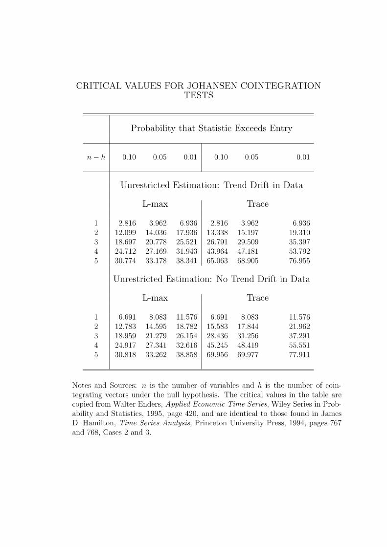
CRITICAL VALUES FOR JOHANSEN COINTEGRATIONTESTS
Probability that Statistic Exceeds Entry
n− h 0.10 0.05 0.01 0.10 0.05 0.01
Unrestricted Estimation: Trend Drift in Data
L-max Trace
1 2.816 3.962 6.936 2.816 3.962 6.9362 12.099 14.036 17.936 13.338 15.197 19.3103 18.697 20.778 25.521 26.791 29.509 35.3974 24.712 27.169 31.943 43.964 47.181 53.7925 30.774 33.178 38.341 65.063 68.905 76.955
Unrestricted Estimation: No Trend Drift in Data
L-max Trace
1 6.691 8.083 11.576 6.691 8.083 11.5762 12.783 14.595 18.782 15.583 17.844 21.9623 18.959 21.279 26.154 28.436 31.256 37.2914 24.917 27.341 32.616 45.245 48.419 55.5515 30.818 33.262 38.858 69.956 69.977 77.911
Notes and Sources: n is the number of variables and h is the number of coin-tegrating vectors under the null hypothesis. The critical values in the table arecopied from Walter Enders, Applied Economic Time Series, Wiley Series in Prob-ability and Statistics, 1995, page 420, and are identical to those found in JamesD. Hamilton, Time Series Analysis, Princeton University Press, 1994, pages 767and 768, Cases 2 and 3.