Econometrica, Vol. 77, No. 3 (May, 2009), 623–685pages.stern.nyu.edu/~dbackus/GE_asset_pricing/Bloom... · Econometrica, Vol. 77, No. 3 (May, 2009), ... leaves open a wide variety

Econometrica, Vol. 77, No. 3 (May, 2009), 623–685

THE IMPACT OF UNCERTAINTY SHOCKS

BY NICHOLAS BLOOM1

Uncertainty appears to jump up after major shocks like the Cuban Missile crisis, theassassination of JFK, the OPEC I oil-price shock, and the 9/11 terrorist attacks. Thispaper offers a structural framework to analyze the impact of these uncertainty shocks.I build a model with a time-varying second moment, which is numerically solved andestimated using firm-level data. The parameterized model is then used to simulate amacro uncertainty shock, which produces a rapid drop and rebound in aggregate out-put and employment. This occurs because higher uncertainty causes firms to temporar-ily pause their investment and hiring. Productivity growth also falls because this pausein activity freezes reallocation across units. In the medium term the increased volatilityfrom the shock induces an overshoot in output, employment, and productivity. Thus,uncertainty shocks generate short sharp recessions and recoveries. This simulated im-pact of an uncertainty shock is compared to vector autoregression estimations on actualdata, showing a good match in both magnitude and timing. The paper also jointly esti-mates labor and capital adjustment costs (both convex and nonconvex). Ignoring capitaladjustment costs is shown to lead to substantial bias, while ignoring labor adjustmentcosts does not.

KEYWORDS: Adjustment costs, uncertainty, real options, labor and investment.

1. INTRODUCTION

UNCERTAINTY APPEARS TO dramatically increase after major economic andpolitical shocks like the Cuban missile crisis, the assassination of JFK, theOPEC I oil-price shock, and the 9/11 terrorist attacks. Figure 1 plots stock-market volatility—one proxy for uncertainty—which displays large bursts ofuncertainty after major shocks, which temporarily double (implied) volatilityon average.2 These volatility shocks are strongly correlated with other mea-sures of uncertainty, like the cross-sectional spread of firm- and industry-levelearnings and productivity growth. Vector autoregression (VAR) estimationssuggest that they also have a large real impact, generating a substantial dropand rebound in output and employment over the following 6 months.

1This article was the main chapter of my Ph.D. thesis, previously called “The Impact of Uncer-tainty Shocks: A Firm-Level Estimation and a 9/11 Simulation.” I would like to thank my advisorsRichard Blundell and John Van Reenen; the co-editor and the referees; my formal discussantsSusantu Basu, Russell Cooper, Janice Eberly, Eduardo Engel, John Haltiwanger, Valerie Ramey,and Chris Sims; Max Floetotto; and many seminar audiences. Financial support of the ESRC andthe Sloan Foundation is gratefully acknowledged.

2In financial markets implied share-returns volatility is the canonical measure for uncertainty.Bloom, Bond, and Van Reenen (2007) showed that firm-level share-returns volatility is signif-icantly correlated with a range of alternative uncertainty proxies, including real sales growthvolatility and the cross-sectional distribution of financial analysts’ forecasts. While Shiller (1981)has argued that the level of stock-price volatility is excessively high, Figure 1 suggests that changesin stock-price volatility are nevertheless linked with real and financial shocks.

© 2009 The Econometric Society DOI: 10.3982/ECTA6248

http://www.econometricsociety.org/

http://www.econometricsociety.org/

http://dx.doi.org/10.3982/ECTA6248

624 NICHOLAS BLOOM

FIGURE 1.—Monthly U.S. stock market volatility. Notes: Chicago Board of Options ExchangeVXO index of percentage implied volatility, on a hypothetical at the money S&P100 option30 days to expiration, from 1986 onward. Pre-1986 the VXO index is unavailable, so actualmonthly returns volatilities are calculated as the monthly standard deviation of the daily S&P500index normalized to the same mean and variance as the VXO index when they overlap from 1986onward. Actual and VXO are correlated at 0.874 over this period. A brief description of the na-ture and exact timing of every shock is contained in Appendix A. The asterisks indicate that forscaling purposes the monthly VXO was capped at 50. Uncapped values for the Black Mondaypeak are 58.2 and for the credit crunch peak are 64.4. LTCM is Long Term Capital Management.

Uncertainty is also a ubiquitous concern of policymakers. For example, af-ter 9/11 the Federal Open Market Committee (FOMC), worried about exactlythe type of real-options effects analyzed in this paper, stated in October 2001that “the events of September 11 produced a marked increase in uncertainty[. . . ] depressing investment by fostering an increasingly widespread wait-and-see attitude.” Similarly, during the credit crunch the FOMC noted that “Sev-eral [survey] participants reported that uncertainty about the economic out-look was leading firms to defer spending projects until prospects for economicactivity became clearer.”

Despite the size and regularity of these second-moment (uncertainty)shocks, there is no model that analyzes their effects. This is surprising giventhe extensive literature on the impact of first-moment (levels) shocks. Thisleaves open a wide variety of questions on the impact of major macroeco-nomic shocks, since these typically have both a first- and a second-momentcomponent.

The primary contribution of this paper is to structurally analyze these typesof uncertainty shocks. This is achieved by extending a standard firm-level

THE IMPACT OF UNCERTAINTY SHOCKS 625

model with a time-varying second moment of the driving process and a mix oflabor and capital adjustment costs. The model yields a central region of inac-tion in hiring and investment space due to nonconvex adjustment costs. Firmsonly hire and invest when business conditions are sufficiently good, and onlyfire and disinvest when they are sufficiently bad. When uncertainty is higher,this region of inaction expands—firms become more cautious in responding tobusiness conditions.

I use this model to simulate the impact of a large temporary uncertaintyshock and find that it generates a rapid drop, rebound, and overshoot in em-ployment, output, and productivity growth. Hiring and investment rates falldramatically in the 4 months after the shock because higher uncertainty in-creases the real-option value to waiting, so firms scale back their plans. Onceuncertainty has subsided, activity quickly bounces back as firms address theirpent-up demand for labor and capital. Aggregate productivity growth also fallsdramatically after the shock because the drop in hiring and investment reducesthe rate of reallocation from low to high productivity firms, which drives themajority of productivity growth in the model as in the real economy.3 Againproductivity growth rapidly bounces back as pent-up reallocation occurs.

In the medium term the increased volatility arising from the uncertaintyshock generates a “volatility overshoot.” The reason is that most firms are lo-cated near their hiring and investment thresholds, above which they hire/investand below which they have a zone of inaction. So small positive shocks gener-ate a hiring and investment response while small negative shocks generate noresponse. Hence, hiring and investment are locally convex in business condi-tions (demand and productivity). The increased volatility of business condi-tions growth after a second-moment shock therefore leads to a medium-termrise in labor and capital.

In sum, these second-moment effects generate a rapid slowdown andbounce-back in economic activity, entirely consistent with the empirical evi-dence. This is very different from the much more persistent slowdown thattypically occurs in response to the type of first-moment productivity and/ordemand shock that is usually modelled in the literature.4 This highlights theimportance to policymakers of distinguishing between the persistent first-moment effects and the temporary second-moment effects of major shocks.

I then evaluate the robustness of these predictions to general equilibrium ef-fects, which for computational reasons are not included in my baseline model.To investigate this I build the falls in interest rates, prices, and wages that oc-cur after actual uncertainty shocks into the simulation. This has little short-runeffect on the simulations, suggesting that the results are robust to general equi-librium effects. The reason is that the rise in uncertainty following a second-moment shock not only generates a slowdown in activity, but it also makes firms

3See Foster, Haltiwanger, and Krizan (2000, 2006).4See, for example, Christiano, Eichenbaum, and Evans (2005) and the references therein.

626 NICHOLAS BLOOM

temporarily extremely insensitive to price changes. This raises a second policyimplication that the economy will be particularly unresponsive to monetary orfiscal policy immediately after an uncertainty shock, suggesting additional cau-tion when thinking about the policy response to these types of events.

The secondary contribution of this paper is to analyze the importance ofjointly modelling labor and capital adjustment costs. For analytical tractabilityand aggregation constraints the empirical literature has estimated either laboror capital adjustment costs individually, assuming the other factor is flexible,or estimated them jointly, assuming only convex adjustment costs.5 I jointlyestimate a mix of labor and capital adjustment costs (both convex and non-convex) by exploiting the properties of homogeneous functions to reduce thestate space. The estimation uses simulated method of moments on firm-leveldata to overcome the identification problem associated with the limited samplesize of macro data. I find moderate nonconvex labor adjustment costs and sub-stantial nonconvex capital adjustment costs. I also find that assuming capitaladjustment costs only—as is standard in the investment literature—generatesan acceptable overall fit, while assuming labor adjustment costs only—as isstandard in the labor demand literature—produces a poor fit.

The analysis of uncertainty shocks links with the earlier work of Bernanke(1983) and Hassler (1996) who highlighted the importance of variations in un-certainty.6 In this paper I quantify and substantially extend their predictionsthrough two major advances: first, by introducing uncertainty as a stochas-tic process which is critical for evaluating the high-frequency impact of majorshocks and, second, by considering a joint mix of labor and capital adjustmentcosts which is critical for understanding the dynamics of employment, invest-ment, and productivity.

This framework also suggests a range of future research. Looking at individ-ual events, it could be used, for example, to analyze the uncertainty impact oftrade reforms, major deregulations, tax changes, or political elections. It alsosuggests there is a trade-off between policy “correctness” and “decisiveness”—it may be better to act decisively (but occasionally incorrectly) than to deliber-

5See, for example: on capital, Cooper and Haltiwanger (1993), Caballero, Engel, and Halti-wanger (1995), Cooper, Haltiwanger, and Power (1999), and Cooper and Haltiwanger (2006); onlabor, Hammermesh (1989), Bertola and Bentolila (1990), Davis and Haltiwanger (1992), Ca-ballero and Engel (1993), Caballero, Engel, and Haltiwanger (1997), and Cooper, Haltiwanger,and Willis (2004); on joint estimation with convex adjustment costs, Shapiro (1986), Hall (2004),and Merz and Yashiv (2007); see Bond and Van Reenen (2007) for a full survey of the literature.

6Bernanke developed an example of uncertainty in an oil cartel for capital investment, whileHassler solved a model with time-varying uncertainty and fixed adjustment costs. There are ofcourse many other linked recent strands of literature, including work on growth and volatilitysuch as Ramey and Ramey (1995) and Aghion, Angeletos, Banerjee, and Manova (2005), oninvestment and uncertainty such as Leahy and Whited (1996) and Bloom, Bond, and Van Reenen(2007), on the business-cycle and uncertainty such as Barlevy (2004) and Gilchrist and Williams(2005), on policy uncertainty such as Adda and Cooper (2000), and on income and consumptionuncertainty such as Meghir and Pistaferri (2004).


ate on policy, generating policy-induced uncertainty. For example, when theFederal Open Markets Committee discussed the negative impact of uncer-tainty after 9/11 it noted that “A key uncertainty in the outlook for investmentspending was the outcome of the ongoing Congressional debate relating to taxincentives for investment in equipment and software” (November 6th, 2001).Hence, in this case Congress’s attempt to revive the economy with tax incen-tives may have been counterproductive due to the increased uncertainty thelengthy policy process induced.

More generally, the framework in this paper also provides one response tothe “where are the negative productivity shocks?” critique of real business cy-cle theories.7 In particular, since second-moment shocks generate large falls inoutput, employment, and productivity growth, it provides an alternative mech-anism to first-moment shocks for generating recessions. Recessions could sim-ply be periods of high uncertainty without negative productivity shocks. En-couragingly, recessions do indeed appear in periods of significantly higher un-certainty, suggesting an uncertainty approach to modelling business cycles (seeBloom, Floetotto, and Jaimovich (2007)). Taking a longer-run perspective thispaper also links to the volatility and growth literature, given the large negativeimpact of uncertainty on output and productivity growth.

The rest of the paper is organized as follows: in Section 2, I empirically in-vestigate the importance of jumps in stock-market volatility; in Section 3, I setup and solve my model of the firm; in Section 4, I characterize the solution ofthe model and present the main simulation results; in Section 5, I outline mysimulated method of moments estimation approach and report the parameterestimates using U.S. firm data; and in Section 6, I run some robustness test onthe simulation results. Finally, Section 7 offers some concluding remarks. Dataand programs are provided in an online supplement (Bloom (2009)).

2. DO JUMPS IN STOCK-MARKET VOLATILITY MATTER?

Two key questions to address before introducing any models of uncertaintyshocks are (i) do jumps8 in the volatility index in Figure 1 correlate with othermeasures of uncertainty and (ii) do these have any impact on real economicoutcomes? In Section 2.1, I address the first question by presenting evidenceshowing that stock-market volatility is strongly linked to other measures of pro-ductivity and demand uncertainty. In Section 2.2, I address the second questionby presenting vector autoregression (VAR) estimations showing that volatil-ity shocks generate a short-run drop in industrial production of 1%, lastingabout 6 months, and a longer-run overshoot. First-moment shocks to the in-terest rates and stock-market levels generate a much more gradual drop and

7See the extensive discussion in King and Rebelo (1999).8I tested for jumps in the volatility series using the bipower variation test of Barndorff-Nielsen

and Shephard (2006) and found statistically significant evidence for jumps. See Appendix A.1.

628 NICHOLAS BLOOM

rebound in activity lasting 2 to 3 years. A full data description for both sectionsis contained in Appendix A.9

2.1. Empirical Evidence on the Links Between Stock-MarketVolatility and Uncertainty

The evidence presented in Table I shows that a number of cross-sectionalmeasures of uncertainty are highly correlated with time-series stock-marketvolatility. Stock-market volatility has also been previously used as a proxy foruncertainty at the firm level (e.g., Leahy and Whited (1996) and Bloom, Bond,and Van Reenen (2007)).

Columns 1–3 of Table I use the cross-sectional standard deviation of firms’pretax profit growth, taken from the quarterly accounts of public companies.As can be seen from column 1 stock-market time-series volatility is stronglycorrelated with the cross-sectional spread of firm-level profit growth. All vari-ables in Table I have been normalized by their standard deviations (SD). Thecoefficient implies that the 2.47 SD rise in stock-market time-series volatilitythat occurred on average after the shocks highlighted in Figure 1 would be as-sociated with a 1.31 SD (1�31 = 2�47 × 0�532) rise in the cross-sectional spreadof the growth rate of profits, a large increase. Column 2 reestimates this in-cluding a full set of quarterly dummies and a time trend, finding very similarresults.10 Column 3 also includes quarterly standard industrial criterion (SIC)three-digit industry controls and again finds similar results,11 suggesting thatidiosyncratic firm-level shocks are driving the time-series variations in volatil-ity.

Columns 4–6 use a monthly cross-sectional stock-return measure and showthat this is also strongly correlated with the stock-return volatility index.Columns 7 and 8 report the results from using the standard deviation of annualfive-factor Total Factor Productivity (TFP) growth within the National Bureauof Economic Research (NBER) manufacturing industry data base. There isalso a large and significant correlation of the cross-sectional spread of industryproductivity growth and stock-market volatility. Finally, columns 9 and 10 usea measure of the dispersion across macro forecasters over their predictions forfuture gross domestic product (GDP), calculated from the Livingstone half-yearly survey of professional forecasters. Once again, periods of high stock-market volatility are significantly correlated with cross-sectional dispersion, inthis case in terms of disagreement across macro forecasters.

9All data and program files are also available at http://www.stanford.edu/~nbloom/.10This helps to control for any secular changes in volatility (see Davis, Haltiwanger, Jarmin,

and Miranda (2006)).11This addresses the type of concerns that Abraham and Katz (1986) raised about Lillien’s

(1982) work on unemployment, where time-series variations in cross-sectional unemploymentappeared to be driven by heterogeneous responses to common macro shocks.

http://www.stanford.edu/~nbloom/

TH

EIM

PAC

TO

FU

NC

ER

TAIN

TY

SHO

CK

S629

TABLE I

THE STOCK-MARKET VOLATILITY INDEX REGRESSED ON CROSS-SECTIONAL MEASURES OF UNCERTAINTYa

Explanatory Variable Is Period by PeriodCross-Sectional Standard Deviation of

Dependent Variable Is Stock-Market Volatilityb

1 2 3 4 5 6 7 8 9 10

Firm profit growth,c Compustat quarterly 0.532 0.526 0.469(0.064) (0.092) (0.115)

Firm stock returns,d CRSP monthly 0.543 0.544 0.570(0.037) (0.038) (0.037)

Industry TFP growth,e SIC 4-digit yearly 0.429 0.419(0.119) (0.125)

GDP forecasts,f Livingstone half-yearly 0.614 0.579(0.111) (0.121)

Time trend No Yes Yes No Yes Yes No Yes No YesMonth/quarter/half-year dummiesg No Yes Yes No Yes Yes n/a n/a No YesControls for SIC 3-digit industryh No No Yes No No Yes n/a n/a n/a n/aR2 0.287 0.301 0.238 0.287 0.339 0.373 0.282 0.284 0.332 0.381Time span 62Q3–05Q1 62M7–06M12 1962–1996 62H2–98H2Average units in cross sectioni 327 355 425 57.4Observations in regression 171 534 35 63

aEach column reports the coefficient from regressing the time series of stock-market volatility on the within period cross-sectional standard deviation (SD) of the explanatoryvariable calculated from an underlying panel. All variables normalized to a SD of 1. Standard errors are given in italics in parentheses below. So, for example, column 1 reportsthat the stock-market volatility index is on average 0.532 SD higher in a quarter when the cross-sectional spread of firms’ profit growth is 1 SD higher.

bThe stock-market volatility index measures monthly volatility on the U.S. stock market and is plotted in Figure 1. The quarterly, half-yearly, and annual values are calculatedby averaging across the months within the period.

cThe standard deviation of firm profit growth measures the within-quarter cross-sectional spread of profit growth rates normalized by average sales, defined as (profitst −profitst−1)/(0�5 × salest + 0�5 × salest−1) and uses firms with 150+ quarters of data in Compustat quarterly accounts.

dThe standard deviation of firm stock returns measures the within month cross-sectional standard deviation of firm-level stock returns for firm with 500+ months of data inthe Center for Research in Securities Prices (CRSP) stock-returns file.

eThe standard deviation of industry TFP growth measures the within-year cross-industry spread of SIC 4-digit manufacturing TFP growth rates, calculated using the five-factorTFP growth figures from the NBER data base.

fThe standard deviation of GDP forecasts comes from the Philadelphia Federal Reserve Bank’s biannual Livingstone survey, calculated as the (standard deviation/mean) offorecasts of nominal GDP 1 year ahead, using half-years with 50+ forecasts, linearly detrended to remove a long-run downward drift.

gMonth/quarter/half-year dummies refers to quarter, month, and half-year controls for period effects.hControls for SIC 3-digit industry denotes that the cross-sectional spread is calculated with SIC 3-digit by period dummies so the profit growth and stock returns are measured

relative to the industry period average.iAverage units in cross section refers to the average number of units (firms, industries, or forecasters) used to measure the cross-sectional spread.

630 NICHOLAS BLOOM

2.2. VAR Estimates on the Impact of Stock-Market Volatility Shocks

To evaluate the impact of uncertainty shocks on real economic outcomesI estimate a range of VARs on monthly data from June 1962 to June2008.12 The variables in the estimation order are log(S&P500 stock mar-ket index), a stock-market volatility indicator (described below), FederalFunds Rate, log(average hourly earnings), log(consumer price index), hours,log(employment), and log(industrial production). This ordering is based onthe assumptions that shocks instantaneously influence the stock market (levelsand volatility), then prices (wages, the consumer price index (CPI), and interestrates), and finally quantities (hours, employment, and output). Including thestock-market levels as the first variable in the VAR ensures the impact of stock-market levels is already controlled for when looking at the impact of volatilityshocks. All variables are Hodrick–Prescott (HP) detrended (λ = 129,600) inthe baseline estimations.

The main stock-market volatility indicator is constructed to take a value 1for each of the shocks labelled in Figure 1 and a 0 otherwise. These 17 shockswere explicitly chosen as those events when the peak of HP detrended volatilitylevel rose significantly above the mean.13 This indicator function is used to en-sure that identification comes only from these large, and arguably exogenous,volatility shocks rather than from the smaller ongoing fluctuations.

Figure 2 plots the impulse response function of industrial production (thesolid line with plus symbols) to a volatility shock. Industrial production displaysa rapid fall of around 1% within 4 months, with a subsequent recovery and re-bound from 7 months after the shock. The 1 standard-error bands (dashedlines) are plotted around this, highlighting that this drop and rebound is sta-tistically significant at the 5% level. For comparison to a first-moment shock,the response to a 1% impulse to the Federal funds rate (FFR) is also plot-ted (solid line with circular symbols), displaying a much more persistent dropand recovery of up to 0.7% over the subsequent 2 years.14 Figure 3 repeats thesame exercise for employment, displaying a similar drop and recovery in activ-ity. Figures A1, A2, and A3 in the Appendix confirm the robustness of theseVAR results to a range of alternative approaches over variable ordering, vari-able inclusion, shock definitions, shock timing, and detrending. In particular,these results are robust to identification from uncertainty shocks defined bythe 10 exogenous shocks arising from wars, OPEC shocks, and terror events.

12Note that this period excludes most of the Credit Crunch, which is too recent to have fullVAR data available. I would like to thank Valerie Ramey and Chris Sims (my discussants) fortheir initial VAR estimations and subsequent discussions.

13The threshold was 1.65 standard deviations above the mean, selected as the 5% one-tailedsignificance level treating each month as an independent observation. The VAR estimation alsouses the full volatility series (which does not require defining shocks) and finds very similar results,as shown in Figure A1.

14The response to a 5% fall the stock-market levels (not plotted) is very similar in size andmagnitude to the response to a 1% rise in the FFR.


FIGURE 2.—VAR estimation of the impact of a volatility shock on industrial production. Notes:Dashed lines are 1 standard-error bands around the response to a volatility shock.

3. MODELLING THE IMPACT OF AN UNCERTAINTY SHOCK

In this section I model the impact of an uncertainty shock. I take a standardmodel of the firm15 and extend it in two ways. First, I introduce uncertaintyas a stochastic process to evaluate the impact of the uncertainty shocks shownin Figure 1. Second, I allow a joint mix of convex and nonconvex adjustmentcosts for both labor and capital. The time-varying uncertainty interacts with

FIGURE 3.—VAR estimation of the impact of a volatility shock on employment. Notes: Dashedlines are 1 standard-error bands around the response to a volatility shock.

15See, for example, Bertola and Caballero (1994), Abel and Eberly (1996), or Caballero andEngel (1999).

632 NICHOLAS BLOOM

the nonconvex adjustment costs to generate time-varying real-option effects,which drive fluctuations in hiring and investment. I also build in temporal andcross-sectional aggregation by assuming firms own large numbers of produc-tion units, which allows me to estimate the model’s parameters on firm-leveldata.

3.1. The Production and Revenue Function

Each production unit has a Cobb–Douglas16 production function

F(A�K�L�H)= AKα(LH)1−α(3.1)

in productivity (A), capital (K), labor (L), and hours (H). The firm faces anisoelastic demand curve with elasticity (ε),

Q = BP−ε�

where B is a (potentially stochastic) demand shifter. These can be combinedinto a revenue function R(A�B�K�L�H)= A1−1/εB1/εKα(1−1/ε)(LH)(1−α)(1−1/ε).For analytical tractability I define a= α(1−1/ε) and b = (1−α)(1−1/ε), andsubstitute A1−a−b = A1−1/εB1/ε, where A combines the unit-level productivityand demand terms into one index, which for expositional simplicity I will referto as business conditions. With these redefinitions we have17

S(A�K�L�H)=A1−a−bKa(LH)b�

Wages are determined by undertime and overtime hours around the standardworking week of 40 hours. Following the approach in Caballero and Engel(1993), this is parameterized as w(H) = w1(1 + w2H

γ), where w1, w2, and γare parameters of the wage equation to be determined empirically.

3.2. The Stochastic Process for Demand and Productivity

I assume business conditions evolve as an augmented geometric randomwalk. Uncertainty shocks are modelled as time variations in the standard devi-ation of the driving process, consistent with the stochastic volatility measure ofuncertainty in Figure 1.

16While I assume a Cobb–Douglas production function, other supermodular homogeneousunit revenue functions could be used. For example, when replacing (3.1) with a constant elas-ticity of substitution aggregator over capital and labor, where F(A�K�L�H) = A(α1K

σ +α2(LH)σ)1/σ , I obtained similar simulation results.

17This reformulation to A as the stochastic variable to yield a jointly homogeneous revenuefunction avoids long-run effects of uncertainty reducing or increasing output because of convexityor concavity in the production function. See Abel and Eberly (1996) for a discussion.


Business conditions are in fact modelled as a multiplicative compositeof three separate random walks18: a macro-level component (AM

t ), a firm-level component (AF

i�t), and a unit-level component (AUi�j�t), where Ai�j�t =

AMt A

Fi�tA

Ui�j�t and i indexes firms, j indexes units, and t indexes time. The macro-

level component is modelled as

AMt =AM

t−1(1 + σt−1WMt )� W M

t ∼ N(0�1)�(3.2)

where σt is the standard deviation of business conditions and W Mt is a macro-

level independent and identically distributed (i.i.d.) normal shock. The firm-level component is modelled as

AFi�t = AF

i�t−1(1 +μi�t + σt−1WFi�t )� W F

i�t ∼ N(0�1)�(3.3)

where μi�t is a firm-level drift in business conditions and W Fi�t is a firm-level

i.i.d. normal shock. The unit-level component is modelled as

AUi�j�t =AU

i�j�t−1(1 + σt−1WUi�j�t)� W U

i�j�t ∼N(0�1)�(3.4)

where W Ui�j�t is a unit-level i.i.d. normal shock. I assume W M

t , W Fi�t , and W U

i�j�t areall independent of each other.

While this demand structure may seem complex, it is formulated to ensurethat (i) units within the same firm have linked investment behavior due to com-mon firm-level business conditions, and (ii) they display some independent be-havior due to the idiosyncratic unit-level shocks, which is essential for smooth-ing under aggregation. This demand structure also assumes that macro-, firm-,and unit-level uncertainty are the same.19 This is broadly consistent with the re-sults from Table I for firm and macro uncertainty, which show these are highly

18A random-walk driving process is assumed for analytical tractability, in that it helps to delivera homogenous value function (details in the next section). It is also consistent with Gibrat’s law.An equally plausible alternative assumption would be a persistent AR(1) process, such as thefollowing based on Cooper and Haltiwanger (2006): log(At) = α + ρ log(At−1) + vt , where vt ∼N(0�σt−1), ρ = 0�885. To investigate this alternative I programmed another monthly simulationwith autoregressive business conditions and no labor adjustment costs (so I could drop the laborstate) and all other modelling assumptions the same. I found in this setup there were still largereal-options effects of uncertainty shocks on output, as plotted in Figure S1 in the supplementalmaterial (Bloom (2009)).

19This formulation also generates business-conditions shocks at the unit level (firm level) thathave three (two) times more variance than at the macro level. This appears to be inconsistent withactual data, since establishment data on things like output and employment are many times morevolatile than the macro equivalent. However, it is worth noting two points. First, micro data alsotypically have much more measurement error than macro data so this could be causing the muchgreater variance of micro data. In stock-returns data, one of the few micro and macro indicatorswith almost no measurement error, firm stock returns have twice the variance of aggregate returnsconsistent with the modelling assumption. Second, because of the nonlinearities in the investmentand hiring response functions (due to nonconvex adjustment costs), output and input growth ismuch more volatile at the unit level than at the macro level, which is smoothed by aggregation. So

634 NICHOLAS BLOOM

correlated. For unit-level uncertainty there is no direct evidence on this, but tothe extent that this assumption does not hold the quantitative impact of macrouncertainty, shocks will be reduced (since total uncertainty will fluctuate lessthan one for one with macro uncertainty), while the qualitative findings willremain. I also evaluate this assumption in Section 6.3 by simulating an uncer-tainty shock which only changes the variance of W M

t (rather than changing thevariance of W M

t , W Fi�t , and W U

i�j�t), with broadly similar results.The firm-level business conditions drift (μi�t) is also assumed to be stochastic

to allow autocorrelated changes over time within firms. This is important forempirically identifying adjustment costs from persistent differences in growthrates across firms, as Section 5 discusses in more detail.

The stochastic volatility process (σ2t ) and the demand conditions drift (μi�t)

are both assumed for simplicity to follow two-point Markov chains

σt ∈ {σL�σH}� where Pr(σt+1 = σj|σt = σk)= πσk�j�(3.5)

μi�t ∈ {μL�μH}� where Pr(μi�t+1 = μj|μi�t = μk)= πμk�j�(3.6)

3.3. Adjustment Costs

The third piece of technology that determines the firms’ activities is the ad-justment costs. There is a large literature on investment and employment ad-justment costs which typically focuses on three terms, all of which I include inmy specification:

Partial Irreversibilities: Labor partial irreversibility, labelled CPL , derives from

per capita hiring, training, and firing costs, and is denominated as a fraction ofannual wages (at the standard working week). For simplicity I assume thesecosts apply equally to gross hiring and gross firing of workers.20 Capital partialirreversibilities arise from resale losses due to transactions costs, the marketfor lemons phenomenon, and the physical costs of resale. The resale loss ofcapital is labelled CP

K and is denominated as a fraction of the relative purchaseprice of capital.

Fixed Disruption Costs: When new workers are added into the productionprocess and new capital is installed, there may be a fixed loss of output. Forexample, adding workers may require fixed costs of advertising, interviewing,and training, or the factory may need to close for a few days while a capitalrefit is occurring. I model these fixed costs as CF

L and CFK for hiring/firing and

investment, respectively, both denominated as fractions of annual sales.

even if the unit-, firm-, and macro-level business conditions processes all have the same variance,the unit- and firm-level employment, capital, and sales growth outcomes will be more volatile dueto more lumpy hiring and investment.

20Micro data evidence, for example, Davis and Haltiwanger (1992), suggests both gross and nethiring/firing costs may be present. For analytical simplicity I have restricted the model to grosscosts, noting that net costs could also be introduced and estimated in future research through theaddition of two net firing cost parameters.


Quadratic Adjustment Costs: The costs of hiring/firing and investment mayalso be related to the rate of adjustment due to higher costs for more rapidchanges, where CQ

LL(EL)2 are the quadratic hiring/firing costs and E denotes

gross hiring/firing, and CQKK( I

K)2 are the quadratic investment costs and I de-

notes gross investment.The combination of all adjustment costs is given by the adjustment cost func-

tion

C(A�K�L�H�I�E�pKt )

= 52w(40)CPL(E

+ +E−)+ (I+ − (1 −CPK)I

−)

+(CF

L1{E �=0} +CFK1{I �=0}

)S(A�K�L�H)

+CQLL

(E

L

)2

+CQKK

(I

K

)2

�

where E+ (I+) and E− (I−) are the absolute values of positive and negativehiring (investment), respectively, and 1{E �=0} and 1{I �=0} are indicator functionswhich equal 1 if true and 0 otherwise. New labor and capital take one periodto enter production due to time to build. This assumption is made to allow meto pre-optimize hours (explained in Section 3.5 below), but is unlikely to playa major role in the simulations given the monthly periodicity. At the end ofeach period there is labor attrition and capital depreciation proportionate toδL and δK , respectively.

3.4. Dealing With Cross-Sectional and Time Aggregation

Gross hiring and investment is typically lumpy with frequent zeros in single-plant establishment-level data, but much smoother and continuous in mul-tiplant establishment and firm-level data. This appears to be because of ex-tensive aggregation across two dimensions: cross-sectional aggregation acrosstypes of capital and production plants; and temporal aggregation across higher-frequency periods within each year. I build this aggregation into the model byexplicitly assuming that firms own a large number of production units and thatthese operate at a higher frequency than yearly. The units can be thought ofas different production plants, different geographic or product markets, or dif-ferent divisions within the same firm.

To solve this model I need to define the relationship between productionunits within the firm. This requires several simplifying assumptions to ensureanalytical tractability. These are not attractive, but are necessary to enable meto derive numerical results and incorporate aggregation into the model. In do-ing this I follow the general stochastic aggregation approach of Bertola andCaballero (1994) and Caballero and Engel (1999) in modelling macro and in-dustry investment, respectively, and most specifically Abel and Eberly (2002)in modelling firm-level investment.

636 NICHOLAS BLOOM

Production units are assumed to independently optimize to determine in-vestment and employment. Thus, all linkages across units within the same firmare modelled by the common shocks to demand, uncertainty, or the price ofcapital. So, to the extent that units are linked over and above these commonshocks, the implicit assumption is that they independently optimize due tobounded rationality and/or localized incentive mechanisms (i.e., managers be-ing assessed only on their own unit’s profit and loss account).21

In the simulation the number of units per firm is set at 250. This numberwas obtained from two pieces of analysis. First, I estimated the number of pro-duction units in my Compustat firms. To do this I started with the work ofDavis et al. (2006), showing that Compustat firms with 500+ employees (in theCensus Bureau data) have on average 185 establishments each in the UnitedStates.22 Their sample is similar to mine, which has Compustat firms with 500+employees and $10m+ of sales (details in Section 5.4). I then used the resultsof Bloom, Schankerman, and Van Reenen (2007), who used Bureau Van Dijkdata to show that for a sample of 715 Compustat firms, 61.5% of their sub-sidiaries are located overseas. Again, their sample is similar to mine, having amedian of 3839 employees compared to 3450 for my sample. Combining thesefacts suggests that—if the number of establishments per subsidiary is approxi-mately the same overseas as in the United States—the Compustat firms in mysample should have around 480 establishments: about 185 in the United Statesand about 295 overseas (295 = 185 × 61�5/(100 − 61�5)).

Second, the simulation results are insensitive to the number of units oncefirms have 250 or more units. The reason is that with 250 units, the firm iseffectively smoothed across independent unit-level shocks, so that more unitsdo not materially change the simulation moments. Since running simulationswith large numbers of units is computationally intensive, I used 250 units as agood approximation to the 480 units my firms approximately have on average.

Of course this assumption on 250 units per firm will have a direct effect onthe estimated adjustment costs (since aggregation and adjustment costs areboth sources of smoothing) and thereby have an indirect effect on the simula-tion. Hence, in Section 5 I reestimate the adjustment costs, assuming insteadthe firm has 1 and 25 units to investigate this further.

The model also assumes no entry or exit for analytical tractability. This seemsacceptable in the monthly time frame (entry/exit accounts for around 2% ofemployment on an annual basis), but is an important assumption to explore infuture research. My intuition is that relaxing this assumption should increase

21The semiindependent operation of plants may be theoretically optimal for incentive reasons(to motivate local managers) and technical reasons (the complexity of centralized informationgathering and processing). The empirical evidence on decentralization in U.S. firms suggests thatplant managers have substantial hiring and investment discretion (see, for example, Bloom andVan Reenen (2007) and Bloom, Sadun, and Van Reenen (2008)).

22I wish to thank Javier Miranda for helping with these figures.


the effect of uncertainty shocks, since entry and exit decisions are extremelynonconvex, although this may have some offsetting effects through the estima-tion of slightly “smoother” adjustment costs.

There is also the issue of time-series aggregation. Shocks and decisions in atypical business unit are likely to occur at a much higher frequency than an-nually, so annual data will be temporally aggregated, and I need to explicitlymodel this. There is little information on the frequency of decision making infirms. The anecdotal evidence suggests monthly frequencies are typical, dueto the need for senior managers to schedule regular meetings, which I assumein my main results.23 Section 5.7 undertakes some robustness tests on this as-sumption and finds that time aggregation is actually quite important. This high-lights the importance of obtaining better data on decision making frequencyfor future research.

3.5. Optimal Investment and Employment

The optimization problem is to maximize the present discounted flow of rev-enues less the wage bill and adjustment costs. As noted above, each unit withinthe firm is assumed to optimize independently. Units are also assumed to berisk neutral to focus on the real-options effects of uncertainty.

Analytical methods suggest that a unique solution to the unit’s optimizationproblem exists that is continuous and strictly increasing in (A�K�L) with analmost everywhere unique policy function.24 The model is too complex, how-ever, to be fully solved using analytical methods, so I use numerical methods,knowing that this solution is convergent with the unique analytical solution.

Given current computing power, however, I have too many state and controlvariables to solve the problem as stated, but the optimization problem can besubstantially simplified in two steps. First, hours are a flexible factor of produc-tion and depend only on the variables (A�K�L), which are predetermined inperiod t given the time to build assumption. Therefore, hours can be optimizedout in a prior step, which reduces the control space by one dimension. Second,the revenue function, adjustment cost function, depreciation schedules, anddemand processes are all jointly homogenous of degree 1 in (A�K�L), allow-ing the whole problem to be normalized by one state variable, reducing thestate space by one dimension.25 I normalize by capital to operate on A

Kand L

K.

These two steps dramatically speed up the numerical simulation, which is run

23Note that even if shocks continuously hit the firm, if decision making only happens monthly,then there is no loss of generality from assuming a monthly shock process.

24The application of Stokey and Lucas (1989) for the continuous, concave, and almost surelybounded normalized returns and cost function in (3.7) for quadratic adjustment costs and partialirreversibilities, and Caballero and Leahy (1996) for the extension to fixed costs.

25The key to this homogeneity result is the random-walk assumption on the demand process.Adjustment costs and depreciation are naturally scaled by unit size, since otherwise units would“outgrow” adjustment costs and depreciation. The demand function is homogeneous through thetrivial renormalization A1−a−b = A1−1/εB1/ε.

638 NICHOLAS BLOOM

on a state space of (AK� LK�σ�μ), making numerical estimation feasible. Appen-

dix B contains a description of the numerical solution method.The Bellman equation of the optimization problem before simplification

(dropping the unit subscripts) can be stated as

V (At�Kt�Lt�σt�μt)

= maxIt �Et �Ht

{S(At�Kt�Lt�Ht)−C(At�Kt�Lt�Ht� It�Et)−w(Ht)Lt

+ 11 + r

E[V (At+1�Kt(1 − δK)+ It�Lt(1 − δL)

+Et�σt+1�μt+1)]}

�

where r is the discount rate and E[·] is the expectation operator. Optimizingover hours and exploiting the homogeneity in (A�K�L) to take out a factorof Kt enables this to be rewritten as

Q(at� lt�σt�μt) = maxit �et

{S∗(at� lt)−C∗(at� lt� it� ltet)(3.7)

+ 1 − δK + it

1 + rE[Q(at+1� lt+1�σt+1�μt+1)]

}�

where the normalized variables are lt = Lt/Kt , at =At/Kt , it = It/Kt , and et =Et/Lt , S∗(at� lt) and C∗(at� lt� it� ltet) are sales and costs after optimization overhours, and Q(at� lt�σt�μt)= V (at�1� lt�σt�μt), which is Tobin’s Q.

4. THE MODEL’S SOLUTION AND SIMULATING AN UNCERTAINTY SHOCK

In this section I present the main results of the model and the uncertaintysimulations. I do this before detailing the parameter values to enable readersto get to the main results more quickly. I list all the parameter values in TablesII and III and discuss how I obtained them in Section 5. Simulation parameterrobustness tests can be found in Section 6.

4.1. The Model’s Solution

The model yields a central region of inaction in (AK� A

L) space, due to the non-

convex costs of adjustment. Units only hire and invest when business conditionsare sufficiently good, and only fire and disinvest when they are sufficiently bad.When uncertainty is higher, these thresholds move out: units become morecautious in responding to business conditions.

To provide some graphical intuition, Figure 4 plots in (AK� A

L) space the val-

ues of the fire and hire thresholds (left and right lines) and the sell and buy


TABLE II

PREDEFINED PARAMETERS IN THE MODEL

Parameter Value Rationale (Also See the Text)

α 1/3 Capital share in output is one-third, labor share is two-thirds.ε 4 33% markup. With constant returns to scale yields a + b = 0�75.

I also try a 20% markup to yield a+ b = 0�833.w1 0�8 Hourly wages minimized at a 40 hour week.w2 2�4e–9 Arbitrary scaling parameter. Set so the wage bill equals unity at

40 hours.σH 2 × σL Uncertainty shocks 2× baseline uncertainty (Figure 1 data). σL es-

timated. I also try 1.5× and 3× baseline shocks.πσ

L�H 1/36 Uncertainty shocks expected every 3 years (17 shocks in 46 years inFigure 1).

πσH�H 0�71 Average 2-month half-life of an uncertainty shock (Figure 1 data).

I also try 1 and 6 month half-lives.(μH +μL)/2 0�02 Average real growth rate equals 2% per year. The spread μH −μL

is estimated.πμ

L�H πμH�L Firm-level demand growth transition matrix assumed symmetric.

The parameter πμH�L estimated.

δK 0�1 Capital depreciation rate assumed 10% per year.δL 0�1 Labor attrition assumed 10% for numerical speed (since δL = δK).

I also try δL = 0�2.r 6�5% Long-run average value for U.S. firm-level discount rate (King and

Rebello (1999)).N 250 Firms operate 250 units, chosen to match data on establishments

per firm. I also try N = 25 and N = 1.

capital thresholds (top and bottom lines) for low uncertainty (σL) and the pre-ferred parameter estimates in Table III column All. The inner region is theregion of inaction (i = 0 and e = 0), where the real-option value of waiting isworth more than the returns to investment and/or hiring. Outside the regionof inaction, investment and hiring will be taking place according to the optimalvalues of i and e. This diagram is a two-dimensional (two-factor) version of theone-dimensional investment models of Abel and Eberly (1996) and Caballeroand Leahy (1996). The gap between the investment/disinvestment thresholdsis higher than between the hire/fire thresholds due to the higher adjustmentcosts of capital.

Figure 5 displays the same lines for both low uncertainty (the inner box oflines) and high uncertainty (the outer box of lines). It can be seen that thecomparative static intuition that higher uncertainty increases real options isconfirmed here, suggesting that large changes in σt can have an important im-pact on investment and hiring behavior.

To quantify the impact of these real-option values I ran the thought exper-iment of calculating what temporary fall in wages and interest rates would berequired to keep units hiring and investment thresholds unchanged when un-

640 NICHOLAS BLOOM

FIGURE 4.—Hiring/firing and investment/disinvestment thresholds. Simulated thresholds us-ing the adjustment cost estimates from the column All in Table III. Although the optimal policiesare of the (s� S) type, it cannot be proven that this is always the case.

certainty temporarily rises from σL to σH . The required wage and interest ratefalls turn out to be quantitatively large: units would need a 25% reduction inwages in periods of high uncertainty to leave their marginal hiring decisions un-changed and a 7% (700 basis point) reduction in the interest rates in periodsof high uncertainty to leave their marginal investment decisions unchanged.26

The reason this uncertainty effect is so large is that labor and capital adjust-ment costs lead units to be cautious about hiring and investing. It is expensiveto hire and then rapidly fire a worker or to buy a piece of equipment and thenquickly resell it. So when uncertainty is high, units optimally postpone hiringand investment decisions for a few months until business conditions becomeclearer.

26This can be graphically seen in supplemental material Figure S2, which plots the low and highuncertainty thresholds, but with the change that when σt = σH , interest rates are 7 percentagepoints lower and wage rates are 25% lower than when σt = σL.


FIGURE 5.—Thresholds at low and high uncertainty. Simulated thresholds using the adjust-ment cost estimates from the column All in Table III. High uncertainty is twice the value of lowuncertainty (σH = 2 × σL).

Interestingly, recomputing these thresholds with permanent (time invariant)differences in uncertainty results in an even stronger impact on the invest-ment and employment thresholds. So the standard comparative static resulton changes in uncertainty will tend to overpredict the expected impact of timechanging uncertainty. The reason is that units evaluate the uncertainty of theirdiscounted value of marginal returns over the lifetime of an investment orhire, so high current uncertainty only matters to the extent that it drives uplong-run uncertainty. When uncertainty is mean reverting, high current val-ues have a lower impact on expected long-run values than if uncertainty wereconstant.

Figure 6 shows a one-dimensional cut of Figure 4 (using the same x-axis),with the level of hiring/firing (solid line, left y-axis) and cross-sectional densityof units (dashed line, right y-axis) plotted. These are drawn for one illustrativeset of parameters: baseline uncertainty (σL), high demand growth (μH), and

642 NICHOLAS BLOOM

FIGURE 6.—The distribution of units between the hiring and firing thresholds. The hiring re-sponse (solid line) and unit-level density (dashed line) for low uncertainty (σL), high drift (μH),and the most common capital/labor (K/L) ratio. The distribution of units in (A/L) space isskewed to the right because productivity growth generates an upward drift in A and attritiongenerates a downward drift in L. The density peaks internally because of lumpy hiring due tofixed costs.

the modal value of capital/labor.27 Three things stand out: first, the distribu-tion is skewed to the right due to positive demand growth and labor attrition;second, the density just below the hiring threshold is low because wheneverthe unit hits the hiring threshold, it undertakes a burst of activity (due to hiringfixed costs) that moves it to the interior of the space; and third, the densitypeaks at the interior which reflects the level of hiring that is optimally under-taken at the hiring threshold.

4.2. The Simulation Outline

The simulation models the impact of a large, but temporary, rise in the vari-ance of business-conditions (productivity and demand) growth. This second-moment shock generates a rapid drop in hiring, investment, and productivity

27Figure 6 is actually a 45◦ cut across Figure 4. The reason is Figure 6 holds K/L constantwhile allowing A to vary.


growth as units become much more cautious due to the rise in uncertainty.Once the uncertainty shock passes, however, activity bounces back as unitsclear their pent-up demand for labor and capital. This also leads to a drop andrebound in productivity growth, since the temporary pause in activity slowsdown the reallocation of labor and capital from low to high productivity units.In the medium term this burst of volatility generates an overshoot in activitydue to the convexity of hiring and investment in business conditions.

Of course this is a stylized simulation, since other factors also typicallychange around major shocks. Some of these factors can and will be added tothe simulation, for example allowing for a simultaneous negative shock to thefirst moment. I start by focusing on a second-moment shock only, however, toisolate the pure uncertainty effects and demonstrate that these alone are capa-ble of generating large short-run fluctuations. I then discuss the robustness ofthis analysis to price changes from general equilibrium effects and a combinedfirst- and second-moment shock. In Section 6 I also show robustness to a rangeof different parameter values, including adjustment costs and the stochasticprocess for uncertainty.

4.3. The Baseline Simulation

I simulate an economy of 1000 units (four firms) for 15 years at a monthlyfrequency. This simulation is then repeated 25,000 times, with the values forlabor, capital, output, and productivity averaged over all these runs. In eachsimulation the model is hit with an uncertainty shock in month 1 of year 11,defined as σt = σH in equation (3.5). All other micro and macro shocks arerandomly drawn as per Section 3. This generates the average impact of an un-certainty shock, where the average is taken over the distribution of micro andmacro shocks. There are both fixed cost and partial irreversibility adjustmentcosts for labor and capital, which are estimated from Compustat data as ex-plained in Section 5 (in particular see the All column in Table III).

Before presenting the simulation results, it is worth first showing the preciseimpulse that will drive the results. Figure 7a reports the average value of σt

normalized to unity before the shock. It is plotted on a monthly basis, with themonth normalized to zero on the date of the shock. Three things are clear fromFigure 7a: first, the uncertainty shock generates a sharp spike in the average σt

across the 25,000 simulations; second, this dies off rapidly with a half-life of2 months; and third, the shock almost doubles average σt (the rise is less than100% because some of the 25,000 simulations already had σt = σH when theshock occurred). In Figure 7b I show the average time path of business condi-tions (Aj�t), showing that the uncertainty shock has no first-moment effect.

In Figure 8, I plot aggregate detrended labor, again normalized to 1 at themonth before the shock. This displays a substantial fall in the 6 months imme-diately after the uncertainty shock and then overshoots from month 8 onward,eventually returning to level by around 3 years.

644 NICHOLAS BLOOM

FIGURE 7A.—The simulation has a large second-moment shock.

The initial drop occurs because the rise in uncertainty increases the real-option value of inaction, leading the majority of units to temporarily freeze

FIGURE 7B.—The simulation has no first moment shock.


FIGURE 8.—Aggregate (detrended) labor drops, rebounds, and overshoots. The aggregate fig-ures for Lt are calculated by summing across all units within the simulation.

hiring. Because of the ongoing exogenous attrition of workers, this generatesa fall in net employment. Endogenizing quits would of course reduce the im-pact of these shocks, since the quit rate would presumably fall after a shock.In the model, to offset this I have conservatively assumed a 10% annual quitrate—well below the 15% to 25% quit rate observed over the business cyclein recent Job Openings and Labor Turnover Survey (JOLTS) data (see Davis,Faberman, and Haltiwanger (2006)). This low fixed quit rate could be thoughtof as the exogenous component due to retirement, maternity, sickness, familyrelocation, and so forth.

The rebound from month 4 onward occurs because of the combination offalling uncertainty (since the shock is only temporary) and rising pent-up de-mand for hiring (because units paused hiring over the previous 3 months). Tomake up the shortfall in labor, units begin to hire at a faster pace than usualso the labor force heads back toward its trend level. This generates the rapidrebound in the total labor from month 3 until about month 6.

4.4. The Volatility Overshoot

One seemingly puzzling phenomenon, however, is the overshoot from month7 onward. Pure real-options effects of uncertainty should generate a drop andovershoot in the growth rate of labor (that is the hiring rate), but only a dropand convergence back to trend in the level of the labor force. So the ques-

646 NICHOLAS BLOOM

tion is what is causing this medium-term overshoot in the level of the laborforce?

This medium-term overshoot arises because the increased volatility of busi-ness conditions leads more units to hit both the hiring and firing thresholds.Since more units are clustered around the hiring threshold than the firingthreshold, due to labor attrition and business-conditions growth (see Figure 6),this leads to a medium-term burst of net hiring. In effect hiring is convex inproductivity just below the hiring threshold—units that receive a small posi-tive shock hire and units that receive a small negative shock do not respond.So total hiring rises in the medium term with the increased volatility of pro-ductivity growth. Of course once units have undertaken a burst of hiring, theyjump to the interior of the region of inaction and so do not hire again forsome time. So in the long-run this results in labor falling back to its long-runtrend path. I label this phenomenon the volatility overshoot, since this medium-term hiring boom is induced by the higher unit-level volatility of business-conditions.28

Thus, the effect of a rise in σt is twofold. First, the real-options effect fromincreased uncertainty over future business conditions causes an initial drop inactivity as units pause investment and hiring. This happens rapidly since ex-pectations change upon impact of the uncertainty shock, so that hiring andinvestment instantly freeze. Second, the effect from increased volatility of re-alized business conditions causes a medium-term hiring boom. This takes moretime to occur because it is driven by the rise in the realized volatility of pro-ductivity growth. This rise in volatility accrues over several months. Thus, theuncertainty drop always precedes the volatility overshoot.

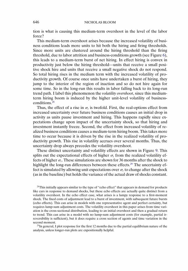
These distinct uncertainty and volatility effects are shown in Figure 9. Thissplits out the expectational effects of higher σt from the realized volatility ef-fects of higher σt . These simulations are shown for 36 months after the shock tohighlight the long-run differences between these effects.29 The uncertainty ef-fect is simulated by allowing unit expectations over σt to change after the shock(as in the baseline) but holds the variance of the actual draw of shocks constant.

28This initially appears similar to the type of “echo effect” that appears in demand for productslike cars in response to demand shocks, but these echo effects are actually quite distinct from avolatility overshoot. In the echo effect case, what arises is a lumpy response to a first-momentshock. The fixed costs of adjustment lead to a burst of investment, with subsequent future bursts(echo effects). This can arise in models with one representative agent and perfect certainty, butrequires lump-sum adjustment costs. The volatility overshoot in this paper arises from time vari-ation is the cross-sectional distribution, leading to an initial overshoot and then a gradual returnto trend. This can arise in a model with no lump-sum adjustment costs (for example, partial ir-reversibility is sufficient), but it does require a cross section of agents and time variation in thesecond moment.

29In general, I plot response for the first 12 months due to the partial equilibrium nature of theanalysis, unless longer-run plots are expositionally helpful.


FIGURE 9.—Separating out the uncertainty and volatility effects. The baseline plot is the sameas in Figure 8 but extended out for 36 months. For the volatility effect only plot, firms haveexpectations set to σt = σL in all periods (i.e., uncertainty effects are turned off), while in theuncertainty effect only, they have the actual shocks drawn from a distribution σt = σL in allperiods (i.e., the volatility effects are turned off).

This generates a drop and rebound back to levels, but no volatility overshoot.The volatility effect is simulated by holding unit expectations over σt constantbut allowing the realized volatility of the business conditions to change afterthe shock (as in the baseline). This generates a volatility overshoot, but no ini-tial drop in activity from a pause in hiring.30 The baseline figure in the graphis simply the aggregate detrended labor (as in Figure 8). This suggests that un-certainty and volatility have very different effects on economic activity, despiteoften being driven by the same underlying phenomena.

The response of aggregate capital to the uncertainty shock is similar to la-bor. There is a short-run drop in capital as units postpone investing, followedby a rebound as they address their pent-up demand for investment, and a sub-sequent volatility driven overshoot (see supplementary material Figure S3).

30In the figure, the volatility effects also take 1 extra month to begin. This is simply becauseof the standard finance timing assumption in (3.2) that σt−1 drives the volatility of Aj�t . Allowingvolatility to be driven by σt delivers similar results because in the short run the uncertainty effectof moving out the hiring and investment thresholds dominates.

648 NICHOLAS BLOOM

4.5. Why Uncertainty Reduces Productivity Growth

Figure 10a plots the time series for the growth of aggregate productivity,defined as

∑j Aj�tLj�t , where the sum is taken over all j production units in

the economy in month t. In this calculation the growth of business conditions(Aj�t) can be used as a proxy for the growth of productivity under the assump-tion that shocks to demand are small in comparison to productivity (or thatthe shocks are independent). Following Baily, Hulten, and Campbell (1992),I define three indices as follows31:∑

Aj�tLj�t −∑

Aj�t−1Lj�t−1∑Aj�t−1Lj�t−1︸︷︷︸

aggregate productivity growth

=∑

(Aj�t −Aj�t−1)Lj�t−1∑Aj�t−1Lj�t−1︸︷︷︸

within productivity growth

+∑

Aj�t(Lj�t −Lj�t−1)∑Aj�t−1Lj�t−1︸︷︷︸

reallocation productivity growth

�

The first term, aggregate productivity growth, is the increase in productivityweighted by employment across units. This can be broken down into two sub-terms: within productivity growth, which measures the productivity increasewithin each production unit (holding the employment of each unit constant),and reallocation productivity growth, which measures the reallocation of em-ployment from low to high productivity units (holding the productivity of eachunit constant).

In Figure 10a aggregate productivity growth shows a large fall after the un-certainty shock. The reason is that uncertainty reduces the shrinkage of lowproductivity units and the expansion of high productivity units, reducing the re-allocation of resources toward more productive units.32 This reallocation fromlow to high productivity units drives the majority of productivity growth in themodel so that higher uncertainty has a first-order effect on productivity growth.This is clear from the decomposition which shows that the fall in total is entirelydriven by the fall in the reallocation term. The within term is constant since, byassumption, the first moment of the demand conditions shocks is unchanged.33

31Strictly speaking, Bailey, Hulten, and Campbell (1992) defined four terms, but for simplicityI have combined the between and cross terms into a reallocation term.

32Formally there is no reallocation in the model because it is partial equilibrium. However, withthe large distribution of contracting and expanding units all experiencing independent shocks,gross changes in unit factor demand are far larger than net changes, with the difference equivalentto reallocation.

33These plots are not completely smooth because the terms are summations of functions whichare approximately squared in Aj�t . For example Aj�tLj�t ≈ λA2

j�t for some scalar λ since Li�t is ap-


FIGURE 10A.—Aggregate productivity growth falls and rebounds after the shock.

FIGURE 10B.—Unit level productivity and hiring for the period before the uncertainty shock.

650 NICHOLAS BLOOM

FIGURE 10C.—Unit level productivity and hiring in the period after the uncertainty shock.

In the bottom two panels this reallocative effect is illustrated by two unit-levelscatter plots of gross hiring against log productivity in the month before theshock (Figure 10b) and the month after the shock (Figure 10c). It can be seenthat after the shock much less reallocative activity takes place with a substan-tially lower fraction of expanding productive units and shrinking unproductiveunits. Since actual U.S. aggregate productivity growth appears to be 70% to80% driven by reallocation,34 these uncertainty effects should play an impor-tant role in the real impact of large uncertainty shocks.

Figure 11 plots the level of an alternative productivity measure—Solow pro-ductivity. This is defined as aggregate output divided by factor share weightedaggregate inputs:

Solow aggregate productivity

=

∑j

A1/(ε−1)j�t Kα

j�t(Lj�t ×Hj�t)1−α

α∑j

Kj�t + (1 − α)∑j

Lj�t ×Hj�t

�

proximately linear in Aj�t . Combined with the random-walk nature of the driving process (whichmeans some individual units grow very large), this results in lumpy aggregate productivity growtheven in very large samples of units.

34Foster, Haltiwanger, and Krizan (2000, 2006) reported that reallocation, broadly defined toinclude entry and exit, accounts for around 50% of manufacturing and 90% of retail productivitygrowth. These figures will in fact underestimate the full contribution of reallocation since theymiss the within establishment reallocation, which Bernard, Redding, and Schott’s (2006) resultson product switching suggests could be substantial.


FIGURE 11.—Solow aggregate productivity (detrended) drops, rebounds, and overshoots.Solow productivity is defined as aggregate output divided by the factor share weighted aggregateinputs.

I report this series because macro productivity measures are typically calcu-lated in this way using only macro data (note that the previous aggregate pro-ductivity measure would require micro data to calculate). As can be seen inFigure 11, the detrended Solow productivity series also falls and rebounds af-ter the uncertainty shock. Again, this initial drop and rebound is because of theinitial pause and subsequent catch-up in the level of reallocation across unitsimmediately after the uncertainty shock. The medium-run overshoot is againdue to the increased level of cross-sectional volatility, which increases the po-tential for reallocation, leading to higher aggregate medium-term productivitygrowth.

Finally, Figure 12 plots the effects of an uncertainty shock on output. Thisshows a clear drop, rebound, and overshoot, very similar to the behavior of thelabor, capital, and productivity. What is striking about Figure 12 is the similar-ity of the size, duration, and time profile of the simulated response to an un-certainty shock compared to the VAR results on actual data shown in Figure 2.In particular, both the simulated and actual data show a drop of detrended ac-tivity of around 1% to 2% after about 3 months, a return to trend at around 6months, and a longer-run gradual overshoot.

652 NICHOLAS BLOOM

FIGURE 12.—Aggregate (detrended) output drops, rebounds, and overshoots.

4.6. Investigating Robustness to General Equilibrium

Ideally I would set up my model within a general equilibrium (GE) frame-work, allowing prices to endogenously change. This could be done, for exam-ple, by assuming agents approximate the cross-sectional distribution of unitswithin the economy using a finite set of moments and then using these mo-ments in a representative consumer framework to compute a recursive com-petitive equilibrium (see, for example, Krusell and Smith (1998), Khan andThomas (2003), and Bachman, Caballero, and Engel (2008)). However, thiswould involve another loop in the routine to match the labor, capital, and out-put markets between units and the consumer, making the program too slowto then loop in the simulated method of moments estimation routine. Hence,there is a trade-off between two options: (i) a GE model with flexible pricesbut assumed adjustment costs35 and (ii) estimated adjustment costs but in afixed price model. Since the effects of uncertainty are sensitive to the nature ofadjustment costs, I chose to take the second option and leave GE analysis tofuture work.

35Unfortunately there are no “off the shelf” adjustment cost estimates that can be used, sinceno paper has previously jointly estimated convex and nonconvex labor and capital adjustmentcosts.


This means the results in this model could be compromised by GE effects iffactor prices changed sufficiently to counteract factor demand changes.36 Oneway to investigate this is to estimate the actual changes in wages, prices, andinterest rates that arise after a stock-market volatility shock and feed theminto the model in an expectations consistent way. If these empirically plausi-ble changes in factor prices radically changed these results, this would suggestthey are not robust to GE, while if they have only a small impact, it is morereassuring on GE robustness.

To do this I use the estimated changes in factor prices from the VAR (seeSection 2.2), which are plotted in Figure 13. An uncertainty shock leads to ashort-run drop and rebound of interest rates of up to 1.1% points (110 basispoint), of prices of up to 0.5%, and of wages of up to 0.3%. I take these num-bers and structurally build them into the model so that when σt = σH , interest

FIGURE 13.—VAR estimation of the impact of a volatility shock on prices. Notes: VARCholesky orthogonalized impulse response functions to a volatility shock. Estimated monthlyfrom June 1962 to June 2008. Impact on the Federal Funds rate is plotted as a percentage pointchange so the shock reduces rates by up to 110 basis points. The impact on the CPI and wages isplotted as percentage change.

36Khan and Thomas (2008) found in their micro to macro investment model that withGE, the response of the economy to productivity shocks is not influenced by the presenceof nonconvex adjustment costs. With a slight abuse of notation this can be characterized as(∂(∂Kt/∂At))/∂NC ≈ 0, where Kt is aggregate capital, At is aggregate productivity, and NCare nonconvex adjustment costs. The focus of my paper on the direct impact of uncertainty onaggregate variables is different and can be characterized instead as ∂Kt/∂σt . Thus, their resultsare not necessarily inconsistent with mine. More recent work by Bachman, Caballero, and En-gel (2008), found their results depend on the choice of parameter values. Sim (2006) built a GEmodel with capital adjustment costs and time-varying uncertainty and found that the impact oftemporary increases in uncertainty on investment is robust to GE effects.

654 NICHOLAS BLOOM

FIGURE 14.—Aggregate (detrended) output: partial equilibrium and pseudo GE. Pseudo-GEallows interest rates, wages, and prices to be 1.1% points, 0.5%, and 0.3%, respectively, lowerduring periods of high uncertainty.

rates are 1.1% lower, prices (of output and capital) are 0.5% lower, and wagesare 0.3% lower. Units expect this to occur, so expectations are rational.

In Figure 14, I plot the level of output after an uncertainty shock with andwithout these “pseudo-GE” prices changes. This reveals two surprising out-comes: first, the effects of these empirically reasonable changes in interestrates, prices, and wages have very little impact on output in the immediate after-math of an uncertainty shock; and second, the limited pseudo-GE effects thatdo occur are greatest at around 3–5 months, when the level of uncertainty (andso the level of the interest rate, price, and wage reductions) is much smaller. Tohighlight the surprising nature of these two findings, Figure S4 (supplementalmaterial) plots the impact of the pseudo-GE price effects on capital, labor, andoutput in a simulation without adjustment costs. In the absence of any adjust-ment costs, these interest rate, prices, and wages changes do have an extremelylarge effect. So the introduction of adjustment costs both dampens and delaysthe response of the economy to the pseudo-GE price changes.

The reason for this limited impact of pseudo-GE price changes is that af-ter an uncertainty shock occurs, the hiring/firing and investment/disinvestmentthresholds jump out, as shown in Figure 5. As a result there are no units nearany of the response thresholds. This makes the economy insensitive to changesin interest rates, prices, or wages. The only way to get an impact would be toshift the thresholds back to the original low uncertainty position where the ma-


jority of units are located, but as noted in Section 4.1 the quantitative impact ofthese uncertainty shocks is equivalent to something like a 7% (700 basis point)higher interest rate and a 25% higher wage rate, so these pseudo-GE price re-ductions of 1.1% in interest rates, 0.5% in prices, and 0.3% in wages are notsufficient to do this.

Of course once the level of uncertainty starts to fall back again, the hir-ing/firing and investment/disinvestment thresholds begin to move back towardtheir low uncertainty values. This means they start to move back toward theregion in (A/K) and (A/L) space where the units are located, so the economybecomes more sensitive to changes in interest rates, prices, and wages. Thus,these pseudo-GE price effects start to play a role, but only with a lag.

In summary, the rise in uncertainty not only reduces levels of labor, capi-tal, productivity, and output, but it also makes the economy temporarily ex-tremely insensitive to changes in factor prices. This is the macro equivalent tothe “cautionary effects” of uncertainty demonstrated on firm-level panel databy Bloom, Bond, and Van Reenen (2007).

For policymakers this is important since it suggests a monetary or fiscal re-sponse to an uncertainty shock is likely to have almost no impact in the imme-diate aftermath of a shock. But as uncertainty falls back down and the economyrebounds, it will become more responsive, so any response to policy will occurwith a lag. Hence, a policymaker trying, for example, to cut interest rates tocounteract the fall in output after an uncertainty shock would find no imme-diate response, but rather a delayed response when the economy was alreadystarting to recover. This cautions against using first-moment policy levers torespond to the second-moment component of shocks; policies aimed directlyat reducing the underlying increase in uncertainty are likely to be far moreeffective.

4.7. A Combined First- and Second-Moment Shock

All the large macro shocks highlighted in Figure 1 comprise both a first-and a second-moment element, suggesting a more realistic simulation wouldanalyze these together. This is undertaken in Figure 15, where the output re-sponse to a pure second-moment shock (from Figure 12) is plotted alongsidethe output response to the same second-moment shock with an additionalfirst-moment shock of −2% to business conditions.37 Adding an additionalfirst-moment shock leaves the main character of the second-moment shockunchanged—a large drop and rebound.

Interestingly, a first-moment shock on its own shows the type of slow re-sponse dynamics that the real data display (see, for example, the response to a

37I choose −2% because this is equivalent to 1 year of business-conditions growth in the model.Larger or smaller shocks yield a proportionally larger or smaller impact.

656 NICHOLAS BLOOM

FIGURE 15.—Combined first- and second-moment shocks. The second-moment shock only hasσt set to σH . The first- and second-moment shock has σt set to σH and also a −2% macro busi-ness-conditions shock. The first-moment shock only just has a −2% macro business-conditionsshock.

monetary shock in Figure 3). This is because the cross-sectional distribution ofunits generates a dynamic response to shocks.38

This rapid drop and rebound in response to a second-moment shock isclearly very different from the persistent drop over several quarters in responseto a more traditional first-moment shock. Thus, to the extent a large shockis more a second-moment phenomenon—for example, 9/11—the response islikely to involve a rapid drop and rebound, while to the extent it is more afirst-moment phenomenon—for example, OPEC II—it is likely to generate apersistent slowdown. However, in the immediate aftermath of these shocks,distinguishing them will be difficult, as both the first- and second-momentcomponents will generate an immediate drop in employment, investment, andproductivity. The analysis in Section 2.1 suggests, however, there are empir-ical proxies for uncertainty that are available in real time to aid policymak-ers, such as the VXO series for implied volatility (see notes to Figure 1), thecross-sectional spread of stock-market returns, and the cross-sectional spreadof professional forecasters.

Of course these first- and second-moment shocks differ both in terms of themoments they impact and in terms of their duration: permanent and tempo-

38See the earlier work on this by, for example, Caballero and Engel (1993) and Bertola andCaballero (1994).


rary, respectively. The reason is that the second-moment component of shocksis almost always temporary while the first-moment component tends to be per-sistent. For completeness a persistent second-moment shock would generatea similar effect on investment and employment as a persistent first-momentshock, but would generate a slowdown in productivity growth through the re-allocation term rather than a one-time reduction in productivity levels throughthe within term. Thus, the temporary/permanent distinction is important forthe predicted time profile of the impact of the shocks on hiring and investment,and the first-/second-moment distinction is important for the route throughwhich these shocks impact productivity.

The only historical example of a persistent second-moment shock wasthe Great Depression, when uncertainty—as measured by share-returnsvolatility—rose to an incredible 130% of 9/11 levels on average for the 4 yearsof 1929 to 1932. While this type of event is unsuitable for analysis using mymodel given the lack of general equilibrium effects and the range of other fac-tors at work, the broad predictions do seem to match up with the evidence.Romer (1990) argued that uncertainty played an important real-options rolein reducing output during the onset of the Great Depression, while Ohanian(2001) and Bresnahan and Raff (1991) reported “inexplicably” low levels ofproductivity growth with an “odd” lack of output reallocation over this period.

5. ESTIMATING THE MODEL PARAMETERS

This section explains how the individual parameter values used to solve themodel and to simulate uncertainty shocks in the previous section were ob-tained. Readers who are focused on the simulation may want to skip to Sec-tion 6.

The full set of parameters is the vector θ that characterizes the firm’s rev-enue function, stochastic processes, adjustment costs, and discount rate. Theeconometric problem consists of estimating this parameter vector θ. Since themodel has no analytical closed form solution, this vector cannot be estimatedusing standard regression techniques. Instead estimation of the parameters isachieved by simulated method of moments (SMM), which minimizes a dis-tance criterion between key moments from actual data (a panel of publiclytraded firms from Compustat) and simulated data. Because SMM is computa-tionally intensive, only 10 parameters can be estimated; the remaining 13 arepredefined.

5.1. Simulated Method of Moments

SMM proceeds as follows: a set of actual data moments ΨA is selected forthe model to match.39 For an arbitrary value of θ the dynamic program is solved

39See McFadden (1989) and Pakes and Pollard (1989) for the statistical properties of the SMMestimator.

658 NICHOLAS BLOOM

and the policy functions are generated. These policy functions are used to cre-ate a simulated data panel of size (κN�T + 10), where κ is a strictly positiveinteger, N is the number of firms in the actual data, and T is the time dimen-sion of the actual data. The first 10 years are discarded so as to start fromthe ergodic distribution. The simulated moments ΨS(θ) are then calculated onthe remaining simulated data panel, along with an associated criterion func-tion Γ (θ), where Γ (θ) = [ΨA − ΨS(θ)]′W [ΨA − ΨS(θ)], which is a weighteddistance between the simulated moments ΨS(θ) and the actual moments ΨA.

The parameter estimate θ is then derived by searching over the parameterspace to find the parameter vector which minimizes the criterion function:

θ = arg minθ∈Θ

[ΨA −ΨS(θ)]′W [ΨA −ΨS(θ)]�(5.1)

Given the potential for discontinuities in the model and the discretization ofthe state space, I use an annealing algorithm for the parameter search (seeAppendix B). Different initial values of θ are selected to ensure the solutionconverges to the global minimum. I also run robustness tests in Section 5.7 withdifferent initial distributions.

The efficient choice for W is the inverse of the variance–covariance matrixof [ΨA −ΨS(θ)]. Defining Ω to be the variance–covariance matrix of the datamoments, Lee and Ingram (1991) showed that under the estimating null, thevariance–covariance of the simulated moments is equal to 1

κΩ. Since ΨA and

ΨS(θ) are independent by construction, W = [(1+ 1κ)Ω]−1, where the first term

in the inner brackets represents the randomness in the actual data and the sec-ond term represents the randomness in the simulated data. Ω is calculated byblock bootstrap with replacement on the actual data. The asymptotic varianceof the efficient estimator θ is proportional to (1+ 1

κ). I use κ = 25, with each of

these 25 firm panels having independent draws of macro shocks. This impliesthe standard error of θ is increased by 4% by using simulation estimation.

5.2. Predefined Parameters

In principle every parameter could be estimated, but in practice the size ofthe estimated parameter space is limited by computational constraints. I there-fore focus on the parameters about which there are probably the weakestpriors—the six adjustment cost parameters, the wage/hours trade-off slope, thebaseline level of uncertainty, and the two key parameters that determine thefirm-level demand drift, Θ = (PRL�FCL�QCL�PRK�FCK�QCK�γ�σL�π

μH�H�

μL). The other 13 parameters are based on values in the data and the litera-ture, and are displayed in Table II.

The predefined parameters outlined in Table II are mostly self-explanatory,although a few require further discussion. One of these is ε, which is the elastic-ity of demand. In a constant returns to scale (CRS) production function setup


this translates directly into the returns to scale parameter on the revenue func-tion, a+ b. There is a wide range of estimates of the revenue returns to scale,recent examples being 0.905 in Khan and Thomas (2003), 0.82 in Bachman,Caballero, and Engel (2008), and 0.592 in Cooper and Haltiwanger (2006).I chose a parameter value of ε = 4, which (under CRS) yields a + b =0.75,which is (i) roughly in the midpoint of this literature and (ii) optimal for thespeed of the numerical simulation since a = 0�25 and b = 0�5 so that capi-tal and labor have integer fraction exponentials which compute much faster.40

This implies a markup of 33%, which is toward the upper end of the range es-timates for price–cost markups. I also check the robustness of my results to aparameter value of a+ b= 0�83 (given by ε= 6 with CRS), which is consistentwith a 20% markup.

The uncertainty process parameters are primarily taken from the macrovolatility process in Figure 1, with the baseline level of uncertainty estimatedin the simulation. The labor attrition rate is chosen at 10% per annum. Thislow figure is selected for two reasons: (i) to be conservative in the simulationsof an uncertainty shock, since attrition drives the fall in employment levels,and (ii) for numerical speed, as this matches the capital depreciation rate, sothat the (L/K) dimension can be ignored if no investment and hiring/firing oc-cur. I also report a robustness test for using an annualized labor attrition rateof 20%, which more closely matches the figures for annualized manufacturingquits in Davis, Faberman, and Haltiwanger (2006).

5.3. Estimation

Under the null, a full-rank set of moments (ΨA) will consistently estimate theparameter of the adjustment costs (Θ).41 The choice of moments is also impor-tant for the efficiency of the estimator. This suggests that moments which are“informative” about the underlying structural parameters should be included.The basic insights of plant- and firm-level data on labor and capital is the pres-ence of highly skewed cross-sectional growth rates and rich time-series dynam-ics, suggesting some combination of cross-sectional and time-series moments.Two additional issues help to guide the exact choice of moments.

5.3.1. Distinguishing the Driving Process From Adjustment Costs

A key challenge in estimating adjustment costs for factor inputs is dis-tinguishing between the dynamics of the driving process and factor adjust-

40Integer fractional exponentials are more easily approximated in binary calculations (see Judd(1998, Chapter 2) for details). This is quantitatively important due to the intensity of exponentialcalculations in the simulation, for example, moving from a+ b = 0�75 to a+ b= 0�76 slows downthe simulation by around 15%. Choosing a lower value of a + b also induces more curvature inthe value function so that less grid points are required to map the relevant space.

41Note that even with a full-rank set of moments the parameters are only identified pointwise.

660 NICHOLAS BLOOM

ment costs. Concentrating on the moments from only one factor—for exam-ple, capital—makes it very hard to do this. To illustrate this, first consider avery smooth driving process without adjustment costs, which would producea smooth investment series. Alternatively consider a volatile driving processwith convex capital adjustment costs, which would also produce a smooth in-vestment series. Hence, without some additional moments (or assumptions),it would be very hard to estimate adjustment costs using just the investmentseries data.

So I focus on the joint (cross-sectional and dynamic) moments of the invest-ment, employment, and sales growth series. The difference in responses acrossthe three series (investment, employment, and sales growth) identifies the twosets of adjustment costs (for capital and labor).42

5.3.2. Distinguishing Persistent Differences From Adjustment Costs

A stylized fact from the estimation of firm- and plant-level investment andlabor demand equations is the empirical importance of “fixed effects,” thatis, persistent differences across firms and plants in their levels of investment,employment, and output growth rates. Without controls for these persistentdifferences, the estimates of the adjustment costs could be biased. For exam-ple, persistent between-firm differences in investment, employment, and salesgrowth rates due to different growth rates of demand would (in the absenceof controls for this) lead to the estimation of large quadratic adjustment costs,which are necessary to induce the required firm-level autocorrelation.

To control for differential firm-level growth rates, the estimator includestwo parameters: the spread of firm-level business-conditions growth, μH −μL,which determines the degree of firm-level heterogeneity in the average growthrates of business conditions as defined in (3.3); and the persistence of firm-levelbusiness-conditions growth, πμ

H�H , as defined in (3.6). When μH − μL is largethere will be large differences in the growth rates of labor, capital, and outputacross firms, and when πμ

H�H is close to unity these will be highly persistent.43 Toidentify these parameters separately from adjustment costs requires informa-tion on the time path of autocorrelation across the investment, employment,and sales growth series. For example, persistent correlations between invest-ment, sales, and employment growth rates going back over many years wouldhelp to identify fixed differences in the growth rates of the driving process,while decaying correlations in the investment series only would suggest convexcapital adjustment costs.

42An alternative is a two-step estimation process in which the driving process is estimated firstand then the adjustment costs are estimated given this driving process (see, for example, Cooperand Haltiwanger (2006)).

43Note that with πμH�H = 1 these will be truly fixed effect differences.


So I include moments for the second-order and fourth-order correlationsof the investment, employment growth, and sales growth series.44 The second-order autocorrelation is chosen to avoid a negative bias in these moments fromunderlying level measurement errors which would arise in a first-order auto-correlation measure, while the fourth-order autocorrelation is chosen to allowa sufficiently large additional time period to pass (2 years) to identify the de-cay in the autocorrelation series. Shorter and longer lags, like the third-order,fifth-order, and sixth-order autocorrelations could also be used, but in experi-mentations did not make much difference.45

5.4. Firm-Level Data

There are too little data at the macroeconomic level to provide sufficientidentification for the model. I therefore identify my parameters using a panelof firm-level data from U.S. Compustat. I select the 20 years of data that cover1981 to 2000.

The data were cleaned to remove major mergers and acquisitions by drop-ping the top and bottom 0.5% of employment growth, sales growth, and invest-ment rates. Firms with an average of at least 500 employees and $10m sales (in2000 prices) were kept to focus on firms which are more size homogeneous.This generated a sample of 2548 firms and 22,950 observations with mean (me-dian) employees of 13,540 (3450) and mean (median) sales of $2247m ($495m)in 2000 prices. In selecting all Compustat firms I am conflating the parameterestimates across a range of different industries, and a strong argument can bemade for running this estimation on an industry by industry basis. However,in the interests of obtaining the “average” parameters for a macro simulationand to ensure a reasonable sample size, I keep the full panel, leaving industry-specific estimation to future work.

Capital stocks for firm i in industry m in year t are constructed by the per-petual inventory method46: labor figures come from company accounts, whilesales figures come from accounts after deflation using the CPI. The invest-ment rate is calculated as (I/K)i�t = Ii�t/(0�5 ∗ (Ki�t +Ki�t−1)), the employmentgrowth rate as (�L/L)i�t = (Li�t −Li�t−1)/(0�5 ∗ (Li�t +Li�t−1)), and the salesgrowth as (�S/S)i�t = (Si�t − Si�t−1)/(0�5 ∗ (Si�t + Si�t−1)).47

44Note: A kth-order correlation for series xi�t and yi�t is defined as Corr(xit � yit−k).45Note that because the optimal weighting matrix takes into account the covariance across

moments, adding extra moments that are highly correlated to included moments has very littleimpact on the parameters estimates.

46Ki�t = (1 − δK)Ki�t−1(Pm�t/Pm�t−1)+ Ii�t , initialized using the net book value of capital, whereIi�t is net capital expenditure on plant, property, and equipment, and Pm�t is the industry-levelcapital goods deflator from Bartelsman, Becker, and Grey (2000).

47Gross investment rates and net employment growth rates are used since these are directlyobserved in the data. Under the null that the model is correctly specified, the choice of net versusgross is not important for the consistency of parameter estimates as long as the same actual andsimulated moments are matched.

662 NICHOLAS BLOOM

The simulated data are constructed in exactly the same way as company ac-counts are built. First, firm value is created by adding up across the N units ineach firm. It is then converted into annual figures using standard accountingtechniques: simulated data for flow figures from the accounting profit & lossand cash-flow statements (such as sales and capital expenditure) are added upacross the 12 months of the year; simulated data for stock figures from the ac-counting balance sheet statement (such as capital stock and labor force) aretaken from the year end values.

By constructing my simulation data in the same manner as company accountsI can estimate adjustment costs using firm-level data sets like Compustat. Thishas some advantages versus using census data sets like the Logitudinal Re-search Dataset (LRD) because firm-level data are (i) easily available to all re-searchers in a range of different countries; (ii) matched into firm level financialand cash-flow data; and (iii) available as a yearly panel stretching back severaldecades (for example to the 1950s in the United States). Thus, this techniqueof explicitly building aggregation into estimators to match against aggregatedquoted firm-level data should have a broader use in other applications. Theobvious disadvantage of using Compustat is it represents only about one-thirdof employment in the United States (Davis et al. (2006)).

5.5. Measurement Errors

Employment figures are often poorly measured in company accounts, typi-cally including all parttime, seasonal, and temporary workers in the total em-ployment figures without any adjustment for hours, usually after heavy round-ing. This problem is then made much worse by the differencing to generategrowth rates.

As a first step toward reducing the sensitivity toward these measurement er-rors, the autocorrelations of growth rates are taken over longer periods (asnoted above). As a second step, I explicitly introduce employment measure-ment error into the simulated moments to try to mimic the bias these imputeinto the actual data moments. To estimate the size of the measurement er-ror, I assume that firm wages (Wit) can be decomposed into Wit = ηtλj�tφiLit ,where ηt is the absolute price level, λj�t is the relative industry wage rate, φi

is a firm-specific salary rate (or skill/seniority mix), and Lit is the average an-nual firm labor force (hours adjusted). I then regress logWit on a full set ofyear dummies, a log of the 4-digit SIC industry average wage from Bartelsman,Becker, and Gray (2000), a full set of firm-specific fixed effects, and logLit .Under my null on the decomposition of Wit the coefficient on logLit will be ap-proximately σ2

L/(σ2L + σ2

ME), where σ2L is the variation in log employment and

σ2ME is the measurement error in log employment. I find a coefficient (standard

error (s.e.)) on logLit of 0.882 (0.007), implying a measurement error of 13%


in the logged labor force numbers.48 This is reassuringly similar to the 8% esti-mate for measurement error in Compustat manufacturing firms’ labor figuresthat Hall (1987) calculated comparing ordinary least squares and instrumen-tal variable estimates. I take the average of these figures and incorporate thisinto the simulation estimation by multiplying the aggregated annual firm laborforce by mei�t , where mei�t ∼ i�i�d� LN(0�0�105) before calculating simulatedmoments.

The other variable which is also potentially affected by measurement error isthe capital stock.49 Actual depreciation rates are not observed, so the perpet-ual inventory capital stock is potentially mismeasured. To investigate the im-portance of this in Section 5.7 I reestimate the model assuming capital stocksalso have a 10% log-normal measurement error.

5.6. Baseline Adjustment-Cost Estimates

In this section I present the estimates of the units’ capital and labor adjust-ment costs. Starting with Table III, the column labelled Data in the bottompanel reports the actual moments from Compustat. These demonstrate thatinvestment rates have a low spread but a heavy right skew, due to the lack ofdisinvestment, and strong dynamic correlations. Labor growth rates are rela-tively variable but unskewed, with weaker dynamic correlations. Sales growthrates have similar moments to those of labor, although slightly lower spreadand higher degree of dynamics correlations.

The column in Table III labelled All presents the results from estimatingthe preferred specification, allowing for all types of adjustment costs. The esti-mated adjustment costs for capital imply a large resale loss of around 34% oncapital, fixed investment costs of 1.5% of annual sales (about 4 working days),and no quadratic adjustment costs. The estimated labor adjustment costs implylimited hiring and firing costs of about 1.8% of annual wages (about 5 workingdays), and a high fixed cost of around 2.1% of annual revenue (about 6 work-ing days), with no quadratic adjustment costs. The standard errors suggest allof these point estimates are statistically significant except for the fixed cost ofcapital adjustment (CF

K).One question is how do these estimates compare to those previously esti-

mated in the literature? Table IV presents a comparison for some other esti-mates from the literature. Three factors stand out: first, there is tremendousvariation is estimated adjustment costs, reflecting the variety of data, tech-niques, and assumptions used in the different papers; second, my estimates

48Adding firm- or industry-specific wage trends reduces the coefficient on logWit , implying aneven higher degree of measurement error. Running the reverse regression of log labor on logwages plus the same controls generates a coefficient (s.e.) of 0.990 (0.008), indicating that theproportional measurement error in wages (a better recorded financial variable) is many timessmaller than that of employment. The regressions are run using 2468 observations on 219 firms.

49Sales and capital expenditure values are usually easier to audit and so much better measured.

664 NICHOLAS BLOOM

TABLE III

ADJUSTMENT COST ESTIMATES (TOP PANEL)a

Adjustment Costs Specification

Estimated Parameters All Capital Labor Quad None

CPK : investment resale loss (%) 33�9 42�7

(6�8) (14�2)CF

K : investment fixed cost (% annual sales) 1�5 1�1(1�5) (0�2)

CQK : capital quadratic adjustment cost (parameter) 0 0�996 4�844

(0�009) (0�044) (454.15)CP

L: per capita hiring/firing cost (% annual wages) 1�8 16�7(0�8) (0�1)

CFL: fixed hiring/firing costs (% annual sales) 2�1 1�1

(0�9) (0�1)CQ

L : labor quadratic adjustment cost (parameter) 0 1�010 0(0�037) (0�017) (0�002)

σL: baseline level of uncertainty 0�443 0�413 0�216 0�171 0�100(0�009) (0�012) (0�005) (0�005) (0�005)

μH −μL: spread of firm business conditions growth 0�121 0�122 0�258 0�082 0�158(0�002) (0�002) (0�001) (0�001) (0�001)

πμH�L: transition of firm business conditions growth 0 0 0�016 0 0�011

(0�001) (0�001) (0�001) (0�001) (0�001)γ : curvature of the hours/wages function 2�093 2�221 3�421 2�000 2�013

(0�272) (0�146) (0�052) (0�009) (14�71)

(Continues)

of positive capital and labor adjustment costs appear broadly consistent withother papers which jointly estimate these; and third, studies which estimatenonconvex adjustment costs report positive and typically very substantial val-ues.

For interpretation, in Table III I also display results for four illustrative re-stricted models. First, a model with capital adjustment costs only, assuminglabor is fully flexible, as is typical in the investment literature. In the Capitalcolumns we see that the fit of the model is worse, as shown by the significantrise in the criterion function from 404 to 625.50 This reduction in fit is primarilydue to the worse fit of the labor moments, suggesting ignoring labor adjustmentcosts is a reasonable approximation for modelling investment. Second, a modelwith labor adjustment costs only—as is typical in the dynamic labor demandliterature—is estimated in the column Labor: the fit is substantially worse. Thissuggests that ignoring capital adjustment costs is problematic. Third, a model

50The χ2 value for 3 degrees of freedom is 7.82, so the column Capital can easily be rejectedagainst the null of All given the difference in criterion values of 221. It is also true, however, thatthe preferred All specification can also be rejected as the true representation of the data giventhat the χ2 value for 10 degrees of freedom is 18.31.


TABLE III

(BOTTOM PANEL)

Moments Data Data Moments − Simulated Moments

Correlation (I/K)i�t with (I/K)i�t−2 0.328 0�060 −0�015 0�049 −0�043 0�148Correlation (I/K)i�t with (I/K)i�t−4 0.258 0�037 0�004 0�088 0�031 0�162Correlation (I/K)i�t with (�L/L)i�t−2 0.208 0�003 −0�025 0�004 −0�056 0�078Correlation (I/K)i�t with (�L/L)i�t−4 0.158 −0�015 −0�009 0�036 0�008 0�091Correlation (I/K)i�t with (�S/S)i�t−2 0.260 −0�023 −0�062 −0�044 −0�102 0�024Correlation (I/K)i�t with (�S/S)i�t−4 0.201 −0�010 −0�024 0�018 −0�036 0�087Standard deviation (I/K)i�t 0.139 −0�010 0�010 −0�012 0�038 0�006Coefficient of skewness (I/K)i�t 1.789 0�004 0�092 1�195 1�311 1�916Correlation (�L/L)i�t with (I/K)i�t−2 0.188 −0�007 0�052 −0�075 0�055 0�053Correlation (�L/L)i�t with (I/K)i�t−4 0.133 −0�021 0�024 −0�061 0�038 0�062Correlation (�L/L)i�t with (�L/L)i�t−2 0.160 0�011 0�083 −0�033 0�071 0�068Correlation (�L/L)i�t with (�L/L)i�t−4 0.108 −0�013 0�054 −0�026 0�045 0�060Correlation (�L/L)i�t with (�S/S)i�t−2 0.193 −0�019 0�063 −0�091 0�064 0�023Correlation (�L/L)i�t with (�S/S)i�t−4 0.152 0�003 0�056 −0�051 0�059 0�063Standard deviation (�L/L)i�t 0.189 −0�022 −0�039 0�001 −0�001 0�005Coefficient of skewness (�L/L)i�t 0.445 −0�136 0�294 −0�013 0�395 0�470Correlation (�S/S)i�t with (I/K)i�t−2 0.203 −0�016 −0�015 −0�164 −0�063 −0�068Correlation (�S/S)i�t with (I/K)i�t−4 0.142 −0�008 −0�010 −0�081 −0�030 −0�027Correlation (�S/S)i�t with (�L/L)i�t−2 0.161 −0�005 0�032 −0�105 −0�024 −0�037Correlation (�S/S)i�t with (�L/L)i�t−4 0.103 −0�015 0�011 −0�054 −0�005 −0�020Correlation (�S/S)i�t with (�S/S)i�t−2 0.207 −0�033 0�002 −0�188 −0�040 −0�158Correlation (�S/S)i�t with (�S/S)i�t−4 0.156 0�002 0�032 −0�071 −0�021 −0�027Standard deviation (�S/S)i�t 0.165 0�004 0�003 0�033 0�051 0�062Coefficient of skewness (�S/S)i�t 0.342 −0�407 −0�075 −0�365 0�178 0�370

Criterion, Γ (θ) 404 625 3618 2798 6922

aThe Data column (bottom panel only) contains the moments from 22,950 observations on investment (I), capital(K), labor (L) and sales (S) for 2548 firms. The other columns contain the adjustment costs estimates (top panel) anddata moments minus the simulated moments (bottom panel) for all adjustment costs (All), just capital adjustmentcosts (Capital), just labor adjustment costs (Labor), just quadratic adjustment costs with 1 unit per firm (Quad), andno adjustment costs (None). So, for example, the number 0.328 at the top of the Data column reports that the second-lag of the autocorrelation of investment in the data is 0.328, and the number 0.060 to the right reports that in the Allspecification the simulated moment is 0.060 less than the data moment (so is 0.268 in total). In the top panel standard-errors are given in italics in parentheses below the point estimates. Parameters were estimated using simulated methodof moments, and standard were errors calculated using numerical derivatives.

with quadratic costs only and no cross-sectional aggregation—as is typical inconvex adjustment-costs models—is estimated in the Quad column, leading toa moderate reduction in fit generated by excessive intertemporal correlationand an inadequate investment skew. Interestingly, industry and aggregate dataare much more autocorrelated and less skewed due to extensive aggregation,suggesting quadratic adjustments costs could be a reasonable approximationat this level. Finally, a model with no adjustment costs is estimated in columnNone. Omitting adjustment costs clearly reduces the model fit. It also biasesthe estimation of the business-conditions process to have much larger firm-

666 NICHOLAS BLOOM

TABLE IV

A COMPARISON WITH OTHER CAPITAL AND LABOR ADJUSTMENT-COST ESTIMATES

Capital Labor

Source PI (%) Fixed (%) Quad PI (%) Fixed (%) Quad

Column All in Table III (this paper) 33�9 1�5 0 1.8 2.1 0Ramey and Shapiro (2001) 40–80Caballero and Engel (1999) 16�5Hayashi (1982) 20Cooper and Haltiwanger (2006) 2�5 20�4 0�049Shapiro (1986) 3 1�33Merz and Yashiv (2007) 14�2 4�2Hall (2004) 0 0Nickell (1986) 8–25Cooper, Haltiwanger, and Willis (2004) 1.7 0

aPI denotes partial irreversibilities, Fixed denotes fixed costs, and Quad denotes quadratic adjustment costs. Miss-ing values indicate no parameter estimated in the main specification. Zeros indicate the parameter was not significantlydifferent from zero. Nickell’s (1986) lower [higher] value is for unskilled [skilled] workers. Shapiro’s (1986) value isa weighted average of (2/3)× 0 for production workers and (1/3)× 4 for nonproduction workers. Merz and Yashiv’s(2007) values are the approximated quadratic adjustment costs at the sample mean. Comparability subject to variationin data sample, estimation technique, and maintained assumptions.

level growth fixed effects and lower variance of the idiosyncratic shocks. Thishelps to highlight the importance of jointly estimating adjustment costs and thedriving process.

In Table III there are also some estimates of the driving process parametersσL, μH − μL, and πμ

H�H , as well as the wage–hours curve parameter γ. Whatis clear is that changes in the adjustment-cost parameters leads to changesin these parameters. For example, the lack of adjustment costs in the col-umn Quad generates an estimated uncertainty parameter of around one-thirdof the baseline All value and a spread in firm-level fixed costs of about two-thirds of the baseline All value. This provides support for the selection of mo-ments that can separately identify the driving process and adjustment-cost pa-rameters.

5.7. Robustness Tests on Adjustment-Cost Estimates

In Table V I run some robustness tests on the modelling assumptions. Thecolumn All repeats the baseline results from Table III for ease of comparison.

The column δL = 0�2 reports the results from reestimating the model witha 20% (rather than 10%) annual attrition rate for labor. This higher rate ofattrition leads to higher estimates of quadratic adjustment costs for labor andcapital, and lower fixed costs for labor. This is because with higher labor attri-tion rates, hiring and firing become more sensitive to current demand shocks(since higher attrition reduces the sensitivity to past shocks). To compensate,the estimated quadratic adjustment-cost estimates are higher and fixed costs

TH

EIM

PAC

TO

FU

NC

ER

TAIN

TY

SHO

CK

S667

TABLE V

ADJUSTMENT COST ROBUSTNESS TESTSa

Adjustment Costs Specification

Estimated Parameters All δL = 20% a+ b = 0�83 N = 25 N = 1 Pre −5% Pre +5% Cap ME Yearly Weekly

CPK : investment resale loss (%) 33�9 28�6 29�8 30�3 47�0 33�9 36�1 35�3 45�3 50�0

(6�8) (4�8) (4�8) (8�7) (9�1) (6�8) (4�9) (5�1) (5�2) (30�8)CFK : investment fixed cost (% annual sales) 1�5 2�1 2�1 0�9 1�3 1�5 1�6 0�9 2�1 1�6

(1�0) (0�9) (0�5) (0�4) (0�2) (1�0) (0�5) (0�4) (0�3) (0�4)CQK : capital quadratic adjustment cost 0 0�461 0 0�616 2�056 0 0�058 0�525 0�025 1�488

(0�009) (0�054) (0�007) (0�154) (0�284) (0�009) (0�037) (0�078) (0�015) (0�729)CPL: per capita hiring/firing cost (% wages) 1�8 1�0 0 0 0 1�8 0 0 2�0 0

(0�8) (0�1) (0�0) (0�1) (0�1) (0�8) (0�04) (0�7) (0�9) (6�1)CFL: fixed hiring/firing costs (% sales) 2�1 0�3 1�7 1�3 0 2�1 1�6 0�9 2�0 1�3

(0�9) (0�1) (0�6) (0�8) (0�0) (0�9) (0�7) (0�4) (0�5) (0�3)CQL : labor quadratic adjustment cost 0 0�360 0 0�199 0�070 0 0 0 1�039 0�808

(0�037) (0�087) (0�021) (0�062) (0�031) (0�037) (0�018) (0�017) (0�165) (0�612)σL: baseline level of uncertainty 0�443 0�490 0�498 0�393 0�248 0�443 0�469 0�515 0�339 0�600

(0�009) (0�019) (0�012) (0�013) (0�008) (0�009) (0�011) (0�017) (0�011) (0�035)μH −μL: spread of business conditions growth 0�121 0�137 0�123 0�163 0�126 0�121 0�132 0�152 0�228 0

(0�002) (0�002) (0�001) (0�002) (0�002) (0�002) (0�002) (0�003) (0�005) (0�018)πμH�L: transition business conditions growth 0 0 0 0 0 0 0 0 0�016 n/a

(0�001) (0�001) (0�001) (0�001) (0�001) (0�001) (0�001) (0�001) (0�001) n/aγ: curvature of hours/wages function 2�093 2�129 2�000 2�148 2�108 2�093 2�056 2�000 2�000 2�129

(0�272) (0�222) (0�353) (0�266) (0�147) (0�272) (0�246) (0�211) (0�166) (0�254)

Criterion, Γ (θ) 404 496 379 556 593 403 380 394 656 52aAdjustment costs estimates using the same methodology as in Table III for the baseline model (All), except 20% annualized labor attrition (δL = 20%), 20% markup

(a + b = 0�83), only 25 units per firm (N = 25), only 1 unit per firm (N = 1), a 5% negative business-conditions shock 6 months prior to the start of the simulation period(pre −5%), a 5% positive business-conditions shock 6 months prior to the simulation period (pre +5%), a 10% log-normal capital measurement error (cap ME), and simulationrun at a yearly frequency (Yearly). The final column (Weekly) is different. This evaluates temporal aggregation bias. It reports parameters estimated using moments from simulateddata created by taking the parameters values from the All column, simulating at a weekly frequency, and then aggregating up to yearly data. This is done to test the bias fromestimating the model assuming an underlying monthly process when in fact the moments are generated from an underlying weekly process. Standard errors are given in Italicsbelow the point estimates.

668 NICHOLAS BLOOM

are lower. The column a+ b = 0�83 reports the results for a specification witha 20% markup, in which the estimated adjustment costs look very similar tothe baseline results.

In columns N = 25 and N = 1, the results are reported for simulations as-suming the firm operates 25 units and 1 unit, respectively.51 These assumptionsalso lead to higher estimates for the quadratic adjustment costs and lower esti-mates for the nonconvex adjustment costs to compensate for the reduction insmoothing by aggregation.

In columns Pre −5% and Pre +5%, the results are reported for simulationsassuming there is a −5% and +5% shock, respectively, to business conditionsin the 6 months before the simulation begins. This simulates running the simu-lation during a recession and boom, respectively, to investigate how the initialconditions influence the results. As shown in Table V the results are numeri-cally identical for Pre −5% and similar for Pre +5% to those for All, suggestingthe results are robust to different initial conditions. The reason is that the longtime period of the simulation (20 years) and the limited persistence of macroshocks means that the impact of initial conditions dies quickly.

In column Cap ME, the parameters are estimated including a log-normal10% measurement error for capital, with broadly similar results. Finally, thelast two columns investigate the impact of time aggregation. First, the columnYearly reports the results for running the simulation at a yearly frequency with-out any time aggregation. Dropping time aggregation leads to higher estimatedquadratic adjustment costs to compensate for the loss of smoothing by aggrega-tion. Second, the column Weekly reports the results from (i) taking the baselineAll parameter estimates and using them to run a weekly frequency simulation,(ii) aggregating these data to a yearly frequency, and (iii) using this to estimatethe model assuming a monthly underlying frequency. Thus, this seeks to under-stand the bias from assuming the model is monthly if the underlying generatingprocess was in fact weekly. Comparing the All parameter values used to gen-erate the data with the Weekly values estimated from (incorrectly) assuming amonthly underlying frequency reveals a number of differences. This highlightsthat modelling time aggregation correctly appears to matter for correctly esti-mating adjustment costs. Given the lack of prior empirical or simulation resultson temporal aggregation, this suggests an area in which further research wouldbe particularly valuable.

6. SIMULATION ROBUSTNESS

In this section, I undertake a set of simulation robustness tests for differentvalues of adjustment costs, the predetermined parameters, and the uncertaintyprocess.

51The specification with N = 1 is included to provide guidance on the impact of simulatedaggregation rather than for empirical realism. The evidence from the annual reports of almost alllarge companies suggests aggregation is pervasive.


6.1. Adjustment Costs

To evaluate the effects of different types of adjustment, I ran three simu-lations: the first with fixed costs only, the second with partial irreversibilitiesonly, and the third with quadratic adjustment costs only.52 The output fromthese three simulations is shown in Figure 16. As can be seen, the two specifi-cations with nonconvex adjustment costs generate a distinct drop and reboundin economic activity. The rebound with fixed costs is faster than with partialirreversibilities because of the bunching in hiring and investment, but other-wise they are remarkably similar in size, duration, and profile. The quadraticadjustment-cost specification appears to generate no response to an uncer-tainty shock. The reason is that there is no kink in adjustment costs aroundzero, so there is no option value associated with doing nothing.

In summary, this suggests the predictions are very sensitive to the inclusionof some degree of nonconvex adjustment costs, but are much less sensitive tothe type (or indeed level) of these nonconvex adjustment costs. This highlights

FIGURE 16.—Different adjustment costs. Adjustment costs in the fixed costs specification haveonly the CF

K and CFL adjustment costs from the All estimation in Table III the partial irreversibility

has only the CPK and CP

L from the baseline All estimation in Table III, and the quadratic has theadjustment costs from the Quad column in Table III.

52For fixed costs and partial irreversibilities the adjustment costs are the fixed cost and partialirreversibility components of the parameter values from the All column in Table III. For quadraticadjustment costs, the values are from the Quad column in Table III.

670 NICHOLAS BLOOM

the importance of the prior step of estimating the size and nature of the un-derlying labor and capital adjustment costs.

6.2. Predefined Parameters

To investigate the robustness of the simulation results to the assumptionsover the predefined parameters, I reran the simulations using the differentparameters from Table V. The results, shown in Figure 17, highlight that thequalitative result of a drop and rebound in activity is robust to the different as-sumptions over the predetermined parameters. This is because of the presenceof some nonconvex component in all the sets of estimated adjustment costs inTable V.

The size of this drop and rebound did vary across specifications, however.Running the simulation with the N = 1 parameter estimates from Table Vleads to a drop of only 1%, about half the baseline drop of about 1.8%. Thissmaller drop was due to the very high levels of estimated quadratic adjustmentcosts that were required to smooth the investment and employment series inthe absence of cross-sectional aggregation. Of course, the assumption of nocross-sectional aggregation (N = 1) is inconsistent with the pervasive aggrega-tion in the typical large firm. This simulation is presented simply to highlightthe importance of building aggregation into estimation routines when it is alsopresent in the data.

FIGURE 17.—Simulation robustness to different parameter assumptions.


In the δL = 0�2 specification the drop was around 2.25%, about 30% abovethe baseline drop, due to the greater labor attrition after the shock. Hence,this more realistic assumption on 20% annual labor attrition (rather than 10%in the baseline) generates a larger drop and rebound in activity. The resultsfor assuming partial cross-sectional aggregation (N = 25), a 20% markup (a+b = 0�83), a preestimation boom (Pre +5%), and capital measurement errors(Cap ME) are all pretty similar to the baseline simulation (which has full cross-sectional aggregation and a 33% markup).

6.3. Durations and Sizes of Uncertainty Shocks

Finally, I also evaluate the effects of robustness of the simulation predictionsto different durations and sizes of uncertainty shocks. In Figure 18, I plot theoutput response to a shorter-lived shock (a 1-month half-life) and a longer-lived shock (a 6-month half-life). Also plotted is the baseline (a 2-month half-life). It is clear that longer-lived shocks generate larger and more persistentfalls in output. The reason is that the pause in hiring and investment lasts forlonger if the rise in uncertainty is more persistent. Of course, because the risein uncertainty is more persistent, the cumulative increase in volatility is alsolarger so that the medium-term “volatility overshoot” is also greater. Hence,more persistent uncertainty shocks generate a larger and more persistent drop,rebound, and overshoot in activity. This is interesting in the context of theGreat Depression, a period in which uncertainty rose to 260% of the baseline

FIGURE 18.—Uncertainty shocks with half-lives (HL) of 1 month, 2 months, and 6 months.

672 NICHOLAS BLOOM

FIGURE 19.—Different sizes of uncertainty shocks. The larger and smaller uncertainty shockshave values of σH equal to 150% and 300% of the σL level (baseline is 200%).

level for over 4 years, which in my (partial equilibrium) model would generatean extremely large and persistent drop in output and employment.

In Figure 19, I plot the output response to a smaller uncertainty shock(σH = 1�5 × σL), a larger uncertainty shock (σH = 3 × σL), and the baselineuncertainty shock (σH = 2 × σL). Surprisingly, the three different sizes of un-certainty shock lead to similar sized drops in activity. The reason is that real-option values are increasing, but concave, in the level of uncertainty,53 so theimpact of a 50% rise in uncertainty on the hiring and investment thresholds isabout two-thirds of the size of the baseline 100% rise in uncertainty. Since thebaseline impact on the hiring and investment thresholds is so large, even two-thirds of this pauses almost all hiring and investment. What is different acrossthe different sizes of shocks, however, is that larger uncertainty shocks gener-ate a larger medium-term volatility overshoot because the cumulative increasein volatility is greater.

Finally, in Figure 20, I evaluate the effects of an uncertainty shock whichonly changes the variance of macro shocks, and not the variance of firm- orunit-level shocks. This changes two things in the simulation. First, overall un-certainty only rises by 33% after a shock, since while macro uncertainty dou-bles, firm and micro uncertainty are unchanged. Despite this the initial drop issimilar to the baseline simulation for a 100% increase in overall uncertainty.

53See Dixit (1993) and Abel and Eberly (1996) for an analytical derivation and discussion.


FIGURE 20.—Macro uncertainty shock only. At month 0 the simulation plot Macro uncertaintyshock only has macro shocks only set to σH at month 0. Firm and unit level shocks are σL at alltimes.

This confirms the results from Figure 19 that even moderately sized uncer-tainty shocks are sufficient to pause activity. Second, there is no cross-sectionalincrease in firm- and unit-level variance, substantially reducing the volatilityovershoot.54

7. CONCLUSIONS

Uncertainty appears to dramatically increase after major economic and po-litical shocks like the Cuban missile crisis, the assassination of JFK, the OPEC Ioil-price shock, and the 9/11 terrorist attacks. If firms have nonconvex adjust-ment costs, these uncertainty shocks will generate powerful real-option effects,driving the dynamics of investment and hiring behavior. These shocks appearto have large real effects: the uncertainty component alone generates a 1%drop and rebound in employment and output over the following 6 months, anda milder long-run overshoot.

This paper offers a structural framework to analyze these types of uncer-tainty shocks, building a model with a time-varying second moment of the

54There is still some volatility overshoot due to the averaging across macro shocks in the25,000 macro draws. The reason for this is that the cross-sectional distribution is right-skewedon average (as shown in Figure 6) so that investment responds more to positive than negativemacro shocks.

674 NICHOLAS BLOOM

driving process, and a mix of labor and capital adjustment costs. The modelis numerically solved and estimated on firm-level data using simulated methodof moments. The parameterized model is then used to simulate a large macrouncertainty shock, which produces a rapid drop and rebound in output, em-ployment, and productivity growth. This is due to the effect of higher uncer-tainty making firms temporarily pause their hiring and investment behavior. Inthe medium term, the increased volatility arising from the uncertainty shockgenerates a volatility overshoot as firms respond to the increased variance ofproductivity shocks, which drives a medium-term overshoot and longer-run re-turn to trend. Hence, the simulated response to uncertainty shocks generatesa drop, rebound, and longer-run overshoot, much the same as their actual em-pirical impact.

This temporary impact of a second-moment shock is different from the typ-ically persistent impact of a first moment shock. While the second-momenteffect has its biggest drop by month 3 and has rebounded by about month 6,persistent first-moment shocks generate falls in activity that last several quar-ters. Thus, for a policymaker in the immediate aftermath of a shock it is criticalto distinguish the relative contributions of the first- and second-moment com-ponents of shocks for predicting the future evolution of output.

The uncertainty shock also induces a strong insensitivity to other economicstimuli. At high levels of uncertainty the real-option value of inaction is verylarge, which makes firms extremely cautious. As a result, the effects of empiri-cally realistic general equilibrium type interest rate, wage, and price falls havea very limited short-run effect on reducing the drop and rebound in activity.This raises a second policy implication, that in the immediate aftermath of anuncertainty shock, monetary or fiscal policy is likely to be particularly ineffec-tive.

This framework also enables a range of future research. Looking at individ-ual events it could be used, for example, to analyze the uncertainty impact ofmajor deregulations, tax changes, trade reforms, or political elections. It alsosuggests there is a trade-off between policy correctness and decisiveness—itmay be better to act decisively (but occasionally incorrectly) than to deliberateon policy, generating policy-induced uncertainty.

More generally these second-moment effects contribute to the “where arethe negative productivity shocks?” debate in the business cycle literature. Itappears that second-moment shocks can generate short sharp drops and re-bounds in output, employment, investment, and productivity growth withoutthe need for a first-moment productivity shock. Thus, recessions could po-tentially be driven by increases in uncertainty. Encouragingly, recessions doindeed appear in periods of significantly higher uncertainty, suggesting an un-certainty approach to modelling business cycles (see Bloom, Floetotto, andJaimovich (2007)). Taking a longer-run perspective, this model also links tothe volatility and growth literature given the evidence for the primary role ofreallocation in productivity growth.


The paper also jointly estimates nonconvex and convex labor and capitaladjustment costs. I find substantial fixed costs of hiring/firing and investment,a large loss from capital resale, and some moderate per-worker hiring/firingcosts. I find no evidence for quadratic investment or hiring/firing adjustmentcosts. I also find that assuming capital adjustment costs only—as is standard inthe investment literature—generates an acceptable overall fit, while assuminglabor adjustment costs only—as is standard in the labor demand literature—produces a poor fit.

APPENDIX A: DATA

All data and Stata do files used to create the empirical Figures 1, 2, and 3 andTable I are available at http://www.stanford.edu/~nbloom/. In this appendixI describe the contents and construction of these data sets.

A.1. Stock-Market Volatility Data

A.1.1. Testing for Jumps in Stock-Market Volatility

To test for jumps in stock-market volatility, I use the nonparametricbipower variation test of Barndorff-Nielsen and Shephard (2006). The testworks for a time series {xt , t = 1�2� � � � �N} by comparing the squared vari-ation, SV = ∑N

t=3(xt − xt−1)2 with the bipower variation, BPV = ∑N

t=3(xt −xt−1)(xt−1 − xt−2). In the limit as dt → 0, if there are no jumps in the data,then E[SV] → E[BPV] since the variation is driven by a continuous process. Ifthere are jumps, however, then E[SV] > E[BPV] since jumps have a squaredimpact on SV but only a linear impact on BPV. Barndorff-Nielsen and Shep-hard (2006) suggested two different test statistics—the linear-jump and theratio-jump test—which have the same asymptotic distribution but differentfinite-sample properties. Using the monthly data from Figure 1, I reject thenull of no jumps at the 2.2% and 1.6% level using the linear and ratio tests,respectively. Using the daily VXO data underlying Figure 1 (available fromJanuary 1986 onward), I reject the null of no jumps using both tests at the0.0% level.

A.1.2. Defining Stock-Market Volatility Shocks

Given the evidence for the existence of stock-market volatility jumps, I needto define what they are. The main measure is an indicator that takes a valueof 1 for each of the 17 events labelled in Figure 1, and 0 otherwise. These17 events are chosen as those with stock-market volatility more than 1.65 stan-dard deviations above the Hodrick–Prescott detrended (λ= 129�600) mean ofthe stock-market volatility series (the raw undetrended series is plotted in Fig-ure 1). While some of these shocks occur in 1 month only, others span multiplemonths so there was a choice over the exact allocation of their timing. I tried


676 NICHOLAS BLOOM

TABLE A.1

MAJOR STOCK-MARKET VOLATILITY SHOCKS

Event Max Volatility First Volatility Type

Cuban missile crisis October 1962 October 1962 TerrorAssassination of JFK November 1963 November 1963 TerrorVietnam buildup August 1966 August 1966 WarCambodia and Kent State May 1970 May 1970 WarOPEC I, Arab–Israeli War December 1973 December 1973 OilFranklin National October 1974 September 1974 EconomicOPEC II November 1978 November 1978 OilAfghanistan, Iran hostages March 1980 March 1980 WarMonetary cycle turning point October 1982 August 1982 EconomicBlack Monday November 1987 October 1987 EconomicGulf War I October 1990 September 1990 WarAsian Crisis November 1997 November 1997 EconomicRussian, LTCM default September 1998 September 1998 Economic9/11 terrorist attack September 2001 September 2001 TerrorWorldcom and Enron September 2002 July 2002 EconomicGulf War II February 2003 February 2003 WarCredit crunch October 2008 August 2007 Economic

two different approaches: the primary approach is to allocate each event to themonth with the largest volatility spike for that event; an alternative approachis to allocate each event to the first month in which volatility went more than2 standard deviations above the HP detrended mean. The events can also becategorized in terms of terror, war, oil, or economic shocks. So a third volatilityindicator uses only the arguably most exogenous terms of terror, war, and oilshocks.

The volatility shock events, their dates under each timing scheme, and theirclassification are shown in Table A.1. It is noticeable from Table A.1 that al-most all the shocks are bad events. So one question for empirical identifica-tion is how distinct are stock-market volatility shocks from stock-market levelsshocks? Fortunately, it turns out that these series do move reasonably inde-pendently because some events—like the Cuban missile crisis—raise volatilitywithout impacting stock-market levels, while others—like hurricane Katrina—generate falls in the stock market without raising volatility. So, for example, thelog detrended stock-market level has a correlation of −0�192 with the main 1/0volatility shock indicator, a correlation of −0�136 with the 1/0 oil, terror, andwar shock indicator, and a −0�340 correlation with the log detrended volatil-ity index itself. Thus, the impact of stock-market volatility can be separatelyidentified from stock-market levels. In the working paper version of this paper(Bloom (2008)), I briefly described each of the 17 volatility shocks shown onFigure 1 to highlight the fact that these are typically linked to real shocks.


A.2. Cross-Sectional Uncertainty Measures

There are four key cross-sectional uncertainty measures:Standard Deviation of Firm-Level Profits Growth: This is measured on a quar-

terly basis using Compustat quarterly accounts. It is the cross-sectional stan-dard deviation of the growth rates of pretax profits (data item 23). Profit growthhas a close fit to productivity and demand growth in homogeneous revenuefunctions, and is one of the few variables to have been continuously reportedin quarterly accounts since the 1960s. This is normalized by the firms’ aver-age sales (data item 2) and is defined as (profitst − profitst−1)/(0�5 × salest +0�5 × salest−1). Only firms with 150 or more quarters of accounts with salesand pretax profit figures are used to minimize the effects of sample composi-tion changes.55 The growth rates are windsorized at the top and bottom 0.05%growth rates to prevent the series from being driven by extreme outliers.

Standard Deviation of Firm-Level Stock Returns: This is measured on amonthly basis using the CRSP data file. It is the cross-sectional standard de-viation of the monthly stock returns. The sample is all firms with 500 or moremonths of stock-returns data. The returns are windsorized at the top and bot-tom 0.5% growth rates to prevent the series from being driven by extremeoutliers.

Standard Deviation of Industry-Level TFP Growth: This is measured on an an-nual basis using the NBER industry data base (Bartelsman, Becker, and Gray(2000)). The cross-sectional spread is defined as the standard deviation of thefive-factor TFP growth rates, taken across all SIC 4-digit manufacturing indus-tries. The complete sample is a balanced panel for 422 of the 425 industries(results are robust to dropping these three industries).

Standard Deviation of GDP Forecasts. This is measured on a half-yearly basisusing the Philadelphia Federal Reserve Bank’s Livingstone survey of profes-sional forecasters. It is defined as the cross-sectional standard deviation of the1-year-ahead GDP forecasts normalized by the mean of the 1-year-ahead GDPforecasts. Only half-years with 50+ forecasts are used to ensure sufficient sam-ple size for the calculations. This series is linearly detrended across the sample(1950–2006) to remove a long-run downward drift of forecaster variance.

A.3. VAR Data

The VAR estimations are run using monthly data from June 1962 throughJune 2008. The full set of VAR variables in the estimation are log industrialproduction in manufacturing (Federal Reserve Board of Governors, season-ally adjusted), employment in manufacturing (BLS, seasonally adjusted), av-erage hours in manufacturing (BLS, seasonally adjusted), log consumer price

55Limiting compositional change helps to address some of the issues raised by Davis, Faber-man, and Haltiwanger (2006), who found rising sales volatility of publicly quoted firms but flatvolatility of privately held firms. I also include a time trend in column 2 of Table I to directlycontrol for this and focus on short-run movements.

678 NICHOLAS BLOOM

FIGURE A1.—VAR robustness to different shock definitions.

index (all urban consumers, seasonally adjusted), log average hourly earningsfor production workers (manufacturing), Federal Funds rate (effective rate,Federal Reserve Board of Governors), a monthly stock-market volatility indi-cator (described below), and the log of the S&P500 stock-market index. Allvariables are HP detrended using a filter value of λ= 129�600.

In Figure A1, the industrial production impulse response function is shownfor four different measures of volatility: the actual series in Figure 1 after HPdetrending (square symbols), the 1/0 volatility indicator with the shocks scaledby the HP detrended series (dot symbols), an alternative volatility indicatorwhich dates shocks by their first month (rather than their highest month) (tri-angle symbols), and a series which only uses the shocks linked to terror, war,and oil (plus symbols). As can be seen, each one of these shock measures gen-erates a rapid drop and rebound in the predicted industrial production. In Fig-ure A2, the VAR results are also shown to be robust to a variety of alternativevariable sets and orderings. The VAR is reestimated using a simple trivariateVAR (the volatility indicator, log employment, and industrial production only)(square symbols) also displays a drop and rebound. The “quadvariate” VAR(the volatility indicator, log stock-market levels, log employment, and indus-trial production) also displays a similar drop and rebound (cross symbols), asdoes the quadvariate VAR with the variable ordering reversed (circular sym-bols). Hence the response of industrial production to a volatility shock ap-pears robust to both the basic selection and the ordering of variables. In Fig-ure A3, I plot the results using different HP detrending filter values: the lin-ear detrended series (λ = ∞) is plotted (square symbols) alongside the base-line detrending (λ = 129�600) (cross symbols) and the “flexible” detrending(λ= 1296). As can be seen, the results again appear robust. I also conducted arange of other experiments, such as adding controls for the oil price (spot priceof West Texas), and found the results to be similar.


FIGURE A2.—VAR robustness to different variable sets and ordering.

APPENDIX B: NUMERICAL SOLUTION METHOD

This appendix describes some of the key steps in the numerical techniquesused to solve the firm’s maximization problem. The full program, which runson Matlab 64-bit, is at http://www.stanford.edu/~nbloom/.

B.1. Value Function Iteration

The objective is to solve the value function (3.7). This value function solu-tion procedure is used in two parts of the paper. The first is in the simulatedmethod of moments estimation of the unknown adjustment cost parameters,

FIGURE A3.—VAR robustness to different variable detrending assumptions.


680 NICHOLAS BLOOM

whereby the value function is repeatedly solved for a variety of different para-meters, the data are simulated, and these moments are used in the parametersearch algorithm. The second is in the simulation where the value function issolved just once—using the estimated parameters choices—and then used tosimulate a panel of 1000 units, repeated 25,000 times. The numerical contrac-tion mapping procedure used to solve the value function in both cases is thesame. This proceeds following three steps:

STEP 1: Choose a grid of points in (a� l�σ�μ) space. Given the log-linearstructure of the demand process, I use a grid of points in (log(a)� log(l)�σ�μ)space. In the log(a) and log(l) dimensions this is equidistantly spaced; inthe σ and μ spacing this is determined by the estimated parameters. Thenormalization by capital in a and l—noting that a = A/K and l = L/K—also requires that the grid spacing in the log(a) and log(l) dimensions bethe same (i.e., ai+1/ai = lj+1/lj , where i� j = 1�2� � � � �N index grid points) sothat the set of investment rates {ai/a1� ai/a2� � � � � ai/aN} maintains the statespace on the grid.56 This equivalency between the grid spaces in the log(a)and log(l) dimensions means that the solution is substantially simplified if thevalues of δK and δL are equal, so that depreciation leaves the log(l) dimen-sion unchanged. When δK and δL are unequal, the difference between themneeds to be an integer of the grid spacing. For the log(a) dimension depreci-ation is added to the drift in the stochastic process, so there is no constrainton δK . Given the conversion to logs, I need to apply the standard Jensen cor-rection to the driving process (3.2), (3.3), and (3.4); for example, for (3.2),log(AM

t )= log(AMt−1)− (σ2

t−1 −σ2L)/2 +σt−1W

Mt . The uncertainty effect on the

drift rate is second order compared to the real-options effect, so the simula-tions are virtually unchanged if this correction is omitted.

I used a grid of 40,000 points (100 × 100 × 2 × 2). I also experimented withfiner and coarser partitions and found that there were some changes in thevalue functions and policy choices as the partition changed, but the character-istics of the solution (i.e., a threshold response space as depicted in Figure 3)were unchanged as long as about 60 or more grid points were used in the log(a)and log(l) dimensions. Hence, the qualitative nature of the simulation resultswas robust to moderate changes in the number of points in the state spacepartition.

STEP 2: Define the value function on the grid of points. This is straightfor-ward for most of the grid, but toward the edge of the grid, due to the random-walk nature of the demand process, this requires taking expectations of thevalue function off the edge of the state space. To address this, an extrapola-tion procedure is used to approximate the value function off the edge of the

56Note that some extreme choices of the investment rate will move the state off the l grid whichinduces an offsetting choice of employment growth rates e to ensure this does not occur.


state space. Under partial irreversibilities and/or fixed costs, the value functionis log-linear outside the zone of inaction, so that as long as the state space isdefined to include the region of inaction, this approximation is exact. Underquadratic adjustment costs the value function, however, is concave so a log-linear approach is only approximately correct. With a sufficiently large statespace, however, the probability of being at a point off the edge of the statespace is very low, so any approximation error will have little impact.

STEP 3: The value function iteration process. First, select a starting valuefor the value function in the first loop. I used the solution for the value func-tion without any adjustment costs, which can be easily derived. In the SMMestimation routine I initially tried using the last solution in the next iteration,but found this could generate instability in the estimations loop. So insteadI always used the same initial value function. The speed of value function iter-ation depends on the modulus of contraction, which with a monthly frequencyand a 6.5% annual discount rate is relatively slow. The number of loops wasfixed at 250, which was chosen to ensure convergence in the policy functions.In practice, value functions typically converge more slowly than the policy func-tion rules associated with them. Thus, it is generally more efficient to stop theiterations when the policy functions have converged, even if the value functionhas not yet fully converged.

B.2. Simulated Method of Moments Estimation

To generate the simulated data for the SMM estimation (used to createΨS(θ) in Equation (5.1)), I simulate an economy with 1000 firms, with 250 unitseach. This is run for 30 years, with the first 10 years discarded to eliminate theeffects of any assumptions on initial conditions. Each firm is randomly assignedan initial drift parameter μL or μH . I run this simulations 25 times to try to av-erage out over the impact of any individual macro shocks. The same seed isalways used in every simulation iteration. I also assume firms are initially dis-tributed equally across μL and μH given the symmetry of the transition matrixfor μi�t . To ensure that first-moment draws have a constant aggregate drift rate,I numerically set∑

i�j

Ai�j�t = exp(μL+μH)/2t∑i�j

Ai�j�0�

consistent with (3.6) as N → ∞, which in smaller samples stops extreme drawsfor individual units from driving macro averages.

I use a simulated annealing algorithm for minimizing the criterion functionin the estimation step in Equation (5.1). This starts with a predefined first andsecond guess. For the third guess onward it takes the best prior guess and ran-domizes from this to generate a new set of parameter guesses. That is, it takes

682 NICHOLAS BLOOM

the best-fit parameters and randomly “jumps off” from this point for its nextguess. Over time the algorithm “cools,” so that the variance of the parameterjumps falls, allowing the estimator to fine tune its parameter estimates aroundthe global best fit. I restart the program with different initial conditions to en-sure the estimator converges to the global minimum. The simulated annealingalgorithm is extremely slow, which is an issue since it restricts the size of theparameter space which can be estimated. Nevertheless, I use this because itis robust to the presence of local minima and discontinuities in the criterionfunction across the parameter space.

To generate the standard errors for the parameter point estimates, I gen-erate numerical derivatives of the simulation moments with respect to theparameters and weight them using the optimal weighting matrix. One prac-tical issue with this is that the value of the numerical derivative, defined asf ′(x) = f (x+ε)−f (x)

ε, is sensitive to the exact value of ε chosen. This is a com-

mon problem with calculating numerical derivatives using simulated data withunderlying discontinuities, arising, for example, from grid-point-defined valuefunctions. To address this, I calculate four values of the numerical derivativefor an ε of +1%, +2.5%, +5%, and −1% of the midpoint of the parameterspace57 and then take the median value of these numerical derivatives. Thishelps to ensure that the numerical derivative is robust to outliers arising fromany discontinuities in the criterion function.

REFERENCES

ABEL, A., AND J. EBERLY (1996): “Optimal Investment With Costly Reversibility,” Review ofEconomic Studies, 63, 581–593. [631,632,639,672]

(2002): “Investment and q With Fixed Costs: An Empirical Analysis,” Mimeo, WhartonSchool, University of Pennsylvania. [635]

ABRAHAM, K., AND L. KATZ (1986): “Cyclical Unemployment: Sectoral Shifts or Aggregate Dis-turbances?” Journal of Political Economy, 94, 507–522. [628]

ADDA, J., AND R. COOPER (2000): “Balladurette and Juppette: A Discrete Analysis of ScrappingSubsidies,” Journal of Political Economy, 108, 778–806. [626]

AGHION, P., G. ANGELETOS, A. BANERJEE, AND K. MANOVA (2005): “Volatility and Growth:Credit Constraints and Productivity-Enhancing Investment,” Working Paper 11349, NBER.[626]

BACHMAN, R., R. CABALLERO, AND E. ENGEL (2008): “Lumpy Investment in Dynamic GeneralEquilibrium,” Mimeo, Yale. [652,653,659]

BAILY, M., C. HULTEN, AND D. CAMPBELL (1992): “Productivity Dynamics in ManufacturingPlants,” Brookings Papers on Economic Activity, 1992, 187–249. [648]

BARLEVY, G. (2004): “The Cost of Business Cycles Under Endogenous Growth,” American Eco-nomic Review, 94, 964–990. [626]

BARNDORFF-NIELSEN, O., AND N. SHEPHARD (2006): “Econometrics of Testing for Jumps inFinancial Economics Using Bipower Variation,” Journal of Financial Econometrics, 4, 1–30.[627,675]

57For example, the midpoint of the parameter space for CFK is taken as 0.01, so that ε is defined

as 0.0001, 0.00025, 0.0005, and −0.0001.

http://www.e-publications.org/srv/ecta/linkserver/setprefs?rfe_id=urn:sici%2F0012-9682%28200905%2977%3A3%3C623%3ATIOUS%3E2.0.CO%3B2-9

http://www.e-publications.org/srv/ecta/linkserver/openurl?rft_dat=bib:1/AbeEbe1996&rfe_id=urn:sici%2F0012-9682%28200905%2977%3A3%3C623%3ATIOUS%3E2.0.CO%3B2-9

http://www.e-publications.org/srv/ecta/linkserver/openurl?rft_dat=bib:3/AbrKat1986&rfe_id=urn:sici%2F0012-9682%28200905%2977%3A3%3C623%3ATIOUS%3E2.0.CO%3B2-9

http://www.e-publications.org/srv/ecta/linkserver/openurl?rft_dat=bib:4/AddCoo2000&rfe_id=urn:sici%2F0012-9682%28200905%2977%3A3%3C623%3ATIOUS%3E2.0.CO%3B2-9

http://www.e-publications.org/srv/ecta/linkserver/openurl?rft_dat=bib:7/Baietal1992&rfe_id=urn:sici%2F0012-9682%28200905%2977%3A3%3C623%3ATIOUS%3E2.0.CO%3B2-9

http://www.e-publications.org/srv/ecta/linkserver/openurl?rft_dat=bib:8/Bar2004&rfe_id=urn:sici%2F0012-9682%28200905%2977%3A3%3C623%3ATIOUS%3E2.0.CO%3B2-9

http://www.e-publications.org/srv/ecta/linkserver/openurl?rft_dat=bib:9/BarShe2006&rfe_id=urn:sici%2F0012-9682%28200905%2977%3A3%3C623%3ATIOUS%3E2.0.CO%3B2-9

http://www.e-publications.org/srv/ecta/linkserver/openurl?rft_dat=bib:1/AbeEbe1996&rfe_id=urn:sici%2F0012-9682%28200905%2977%3A3%3C623%3ATIOUS%3E2.0.CO%3B2-9

http://www.e-publications.org/srv/ecta/linkserver/openurl?rft_dat=bib:3/AbrKat1986&rfe_id=urn:sici%2F0012-9682%28200905%2977%3A3%3C623%3ATIOUS%3E2.0.CO%3B2-9

http://www.e-publications.org/srv/ecta/linkserver/openurl?rft_dat=bib:4/AddCoo2000&rfe_id=urn:sici%2F0012-9682%28200905%2977%3A3%3C623%3ATIOUS%3E2.0.CO%3B2-9

http://www.e-publications.org/srv/ecta/linkserver/openurl?rft_dat=bib:7/Baietal1992&rfe_id=urn:sici%2F0012-9682%28200905%2977%3A3%3C623%3ATIOUS%3E2.0.CO%3B2-9

http://www.e-publications.org/srv/ecta/linkserver/openurl?rft_dat=bib:8/Bar2004&rfe_id=urn:sici%2F0012-9682%28200905%2977%3A3%3C623%3ATIOUS%3E2.0.CO%3B2-9

http://www.e-publications.org/srv/ecta/linkserver/openurl?rft_dat=bib:9/BarShe2006&rfe_id=urn:sici%2F0012-9682%28200905%2977%3A3%3C623%3ATIOUS%3E2.0.CO%3B2-9


BARTELSMAN, E., R. BECKER, AND W. GRAY (2000): “NBER Productivity Database,” availableat www.nber.org. [661,662,677]

BERNANKE, B. (1983): “Irreversibility, Uncertainty and Cyclical Investment,” Quarterly Journalof Economics, 98, 85–106. [626]

BERNARD, A., S. REDDING, AND P. SCHOTT (2006): “Multi-Product Firms and Product Switch-ing,” Working Paper 12293, NBER. [650]

BERTOLA, G., AND S. BENTOLILA (1990): “Firing Costs and Labor Demand: How Bad Is Eu-rosclerosis,” Review of Economic Studies, 54, 318–402. [626]

BERTOLA, G., AND R. CABALLERO (1994): “Irreversibility and Aggregate Investment,” Review ofEconomic Studies, 61, 223–246. [631,635,656]

BLOOM, N. (2008): “The Impact of Uncertainty Shocks,” Working Paper 13385, NBER. [676](2009): “Supplement to ‘The Impact of Uncertainty Shocks’,” Econometrica Supple-

mental Material, 77, http://econometricsociety.org/ecta/Supmat/6248_data and programs.zip.[627,633]

BLOOM, N., S. BOND, AND J. VAN REENEN (2007): “Uncertainty and Investment Dynamics,”Review of Economic Studies, 74, 391–415. [623,626,628,655]

BLOOM, N., M. FLOETOTTO, AND N. JAIMOVICH (2007): “Really Uncertain Business Cycles,”Mimeo, Stanford. [627,674]

BLOOM, N., R. SADUN, AND J. VAN REENEN (2008): “The Organization of Firms Across Coun-tries,” Mimeo, LSE. [636]

BLOOM, N., M. SCHANKERMAN, AND J. VAN REENEN (2007): “Identifying Technology Spilloversand Product Market Rivalry,” Working Paper 13060, NBER. [636]

BLOOM, N., AND J. VAN REENEN (2007): “Measuring and Explaining Management PracticesAcross Firms and Countries,” Quarterly Journal of Economics, 122, 1351–1408. [636]

BOND, S., AND J. VAN REENEN (2007): “Microeconometric Models of Investment and Employ-ment,” in Handbook of Econometrics (forthcoming). [626]

BRESNAHAN, T., AND D. RAFF (1991): “Intra-Industry Heterogeneity and the Great Depression:The American Motor Vehicles Industry, 1929–1935,” Journal of Economic History, 51, 317–331.[657]

CABALLERO, R., AND E. ENGEL (1993): “Microeconomic Adjustment Hazards and AggregateDynamics,” Quarterly Journal of Economics, 108, 359–383. [626,632,656]

(1999): “Explaining Investment Dynamics in U.S. Manufacturing: A Generalized (S� s)Approach,” Econometrica, 67, 783–826. [631,635,666]

CABALLERO, R., E. ENGEL, AND J. HALTIWANGER (1995): “Plant-Level Adjustment and Aggre-gate Investment Dynamics,” Brookings Papers on Economic Activity, 2, 1–54. [626]

(1997): “Aggregate Employment Dynamics: Building From Microeconomics Evidence,”American Economic Review, 87, 115–137. [626]

CABALLERO, R., AND J. LEAHY (1996): “Fixed Costs: The Demise of Marginal Q,” WorkingPaper 5508, NBER. [637,639]

CHRISTIANO, L., M. EICHENBAUM, AND C. EVANS (2005): “Nominal Rigidities and the DynamicEffects of a Shock to Monetary Policy,” Journal of Political Economy, 113, 1–45. [625]

COOPER, R., AND J. HALTIWANGER (1993): “The Aggregate Implications of Machine Replace-ment: Theory and Evidence,” American Economic Review, 83, 360–382. [626]

(2006): “On the Nature of the Capital Adjustment Process,” Review of Economic Studies,73, 611–633. [626,633,659,660,666]

COOPER, R., J. HALTIWANGER, AND J. WILLIS (2004): “Dynamics of Labor Demand: EvidenceFrom Plant-Level Observations and Aggregate Implications,” Working Paper 10297, NBER.[626,666]

COOPER, R., J. HALTIWANGER, AND L. POWER (1999): “Machine Replacement and the BusinessCycle: Lumps and Bumps,” American Economic Review, 89, 921–946. [626]

DAVIS, S., R. FABERMAN, AND J. HALTIWANGER (2006): “The Flow Approach to Labor Markets:New Data Sources and Micro–Macro Links,” Journal of Economic Perspectives, 20, 3–26. [645,659,677]

http://www.nber.org

http://www.e-publications.org/srv/ecta/linkserver/openurl?rft_dat=bib:11/Ber1983&rfe_id=urn:sici%2F0012-9682%28200905%2977%3A3%3C623%3ATIOUS%3E2.0.CO%3B2-9

http://www.e-publications.org/srv/ecta/linkserver/openurl?rft_dat=bib:13/BerBen1990&rfe_id=urn:sici%2F0012-9682%28200905%2977%3A3%3C623%3ATIOUS%3E2.0.CO%3B2-9

http://www.e-publications.org/srv/ecta/linkserver/openurl?rft_dat=bib:14/BerCab1994&rfe_id=urn:sici%2F0012-9682%28200905%2977%3A3%3C623%3ATIOUS%3E2.0.CO%3B2-9

http://econometricsociety.org/ecta/Supmat/6248_data%20and%20programs.zip

http://www.e-publications.org/srv/ecta/linkserver/openurl?rft_dat=bib:17/Bloetal2007&rfe_id=urn:sici%2F0012-9682%28200905%2977%3A3%3C623%3ATIOUS%3E2.0.CO%3B2-9

http://www.e-publications.org/srv/ecta/linkserver/openurl?rft_dat=bib:21/BloVAN2007&rfe_id=urn:sici%2F0012-9682%28200905%2977%3A3%3C623%3ATIOUS%3E2.0.CO%3B2-9

http://www.e-publications.org/srv/ecta/linkserver/openurl?rft_dat=bib:22/BonVAN2007&rfe_id=urn:sici%2F0012-9682%28200905%2977%3A3%3C623%3ATIOUS%3E2.0.CO%3B2-9

http://www.e-publications.org/srv/ecta/linkserver/openurl?rft_dat=bib:23/BreRaf1991&rfe_id=urn:sici%2F0012-9682%28200905%2977%3A3%3C623%3ATIOUS%3E2.0.CO%3B2-9

http://www.e-publications.org/srv/ecta/linkserver/openurl?rft_dat=bib:24/CabEng1993&rfe_id=urn:sici%2F0012-9682%28200905%2977%3A3%3C623%3ATIOUS%3E2.0.CO%3B2-9


http://www.e-publications.org/srv/ecta/linkserver/openurl?rft_dat=bib:26/Cabetal1995&rfe_id=urn:sici%2F0012-9682%28200905%2977%3A3%3C623%3ATIOUS%3E2.0.CO%3B2-9


http://www.e-publications.org/srv/ecta/linkserver/openurl?rft_dat=bib:29/Chretal2005&rfe_id=urn:sici%2F0012-9682%28200905%2977%3A3%3C623%3ATIOUS%3E2.0.CO%3B2-9

http://www.e-publications.org/srv/ecta/linkserver/openurl?rft_dat=bib:30/CooHal1993&rfe_id=urn:sici%2F0012-9682%28200905%2977%3A3%3C623%3ATIOUS%3E2.0.CO%3B2-9


http://www.e-publications.org/srv/ecta/linkserver/openurl?rft_dat=bib:33/Cooetal1999&rfe_id=urn:sici%2F0012-9682%28200905%2977%3A3%3C623%3ATIOUS%3E2.0.CO%3B2-9

http://www.e-publications.org/srv/ecta/linkserver/openurl?rft_dat=bib:34/DavFabHaletal2006&rfe_id=urn:sici%2F0012-9682%28200905%2977%3A3%3C623%3ATIOUS%3E2.0.CO%3B2-9

http://www.e-publications.org/srv/ecta/linkserver/openurl?rft_dat=bib:11/Ber1983&rfe_id=urn:sici%2F0012-9682%28200905%2977%3A3%3C623%3ATIOUS%3E2.0.CO%3B2-9

http://www.e-publications.org/srv/ecta/linkserver/openurl?rft_dat=bib:13/BerBen1990&rfe_id=urn:sici%2F0012-9682%28200905%2977%3A3%3C623%3ATIOUS%3E2.0.CO%3B2-9

http://www.e-publications.org/srv/ecta/linkserver/openurl?rft_dat=bib:14/BerCab1994&rfe_id=urn:sici%2F0012-9682%28200905%2977%3A3%3C623%3ATIOUS%3E2.0.CO%3B2-9

http://www.e-publications.org/srv/ecta/linkserver/openurl?rft_dat=bib:17/Bloetal2007&rfe_id=urn:sici%2F0012-9682%28200905%2977%3A3%3C623%3ATIOUS%3E2.0.CO%3B2-9

http://www.e-publications.org/srv/ecta/linkserver/openurl?rft_dat=bib:21/BloVAN2007&rfe_id=urn:sici%2F0012-9682%28200905%2977%3A3%3C623%3ATIOUS%3E2.0.CO%3B2-9

http://www.e-publications.org/srv/ecta/linkserver/openurl?rft_dat=bib:22/BonVAN2007&rfe_id=urn:sici%2F0012-9682%28200905%2977%3A3%3C623%3ATIOUS%3E2.0.CO%3B2-9

http://www.e-publications.org/srv/ecta/linkserver/openurl?rft_dat=bib:23/BreRaf1991&rfe_id=urn:sici%2F0012-9682%28200905%2977%3A3%3C623%3ATIOUS%3E2.0.CO%3B2-9







http://www.e-publications.org/srv/ecta/linkserver/openurl?rft_dat=bib:29/Chretal2005&rfe_id=urn:sici%2F0012-9682%28200905%2977%3A3%3C623%3ATIOUS%3E2.0.CO%3B2-9




http://www.e-publications.org/srv/ecta/linkserver/openurl?rft_dat=bib:33/Cooetal1999&rfe_id=urn:sici%2F0012-9682%28200905%2977%3A3%3C623%3ATIOUS%3E2.0.CO%3B2-9

http://www.e-publications.org/srv/ecta/linkserver/openurl?rft_dat=bib:34/DavFabHaletal2006&rfe_id=urn:sici%2F0012-9682%28200905%2977%3A3%3C623%3ATIOUS%3E2.0.CO%3B2-9

684 NICHOLAS BLOOM

DAVIS, S., AND J. HALTIWANGER (1992): “Gross Job Creation, Gross Job Destruction, and Em-ployment Reallocation,” Quarterly Journal of Economics, 107, 819–863. [626,634]

DAVIS, S., J. HALTIWANGER, R. JARMIN, AND J. MIRANDA (2006): “Volatility and Dispersion inBusiness Growth Rates: Publicly Traded versus Privately Held Firms,” Working Paper 12354,NBER. [628,636,662]

DIXIT, A. (1993): The Art of Smooth Pasting, Fundamentals of Pure and Applied Economics. Read-ing, U.K.: Harwood Academic. [672]

DIXIT, A., AND R. PINDYCK (1994): Investment Under Uncertainty. Princeton, NJ: Princeton Uni-versity Press.

FOSTER, L., J. HALTIWANGER, AND C. KRIZAN (2000): “Aggregate Productivity Growth: LessonsFrom Microeconomic Evidence,” in New Developments in Productivity Analysis. Chicago, IL:University of Chicago Press. [625,650]

(2006): “Market Selection, Reallocation and Restructuring in the U.S. Retail TradeSector in the 1990s,” Review of Economics and Statistics, 88, 748–758. [625,650]

GILCHRIST, S., AND J. WILLIAMS (2005): “Investment, Capacity and Uncertainty: A Putty–ClayApproach,” Review of Economic Dynamics, 8, 1–27. [626]

HALL, B. (1987): “The Relationship Between Firm Size and Firm Growth in the U.S. Manufac-turing Sector,” Journal of Industrial Economics, 35, 583–606. [663]

HALL, R. (2004): “Measuring Factor Adjustment Costs,” Quarterly Journal of Economics, 119,899–927. [626,666]

HAMERMESH, D. (1989): “Labor Demand and the Structure of Adjustment Costs,” AmericanEconomic Review, 79, 674–89. [626]

HASSLER, J. (1996): “Variations in Risk and Fluctuations in Demand—A Theoretical Model,”Journal of Economic Dynamics and Control, 20, 1115–1143. [626]

HAYASHI, F. (1982): “Tobin’s Marginal Q and Average Q: A Neoclassical Interpretation,” Econo-metrica, 50, 213–224. [666]

JUDD, K. (1998): Numerical Methods in Economics. Cambridge, MA: MIT Press. [659]KHAN, A., AND J. THOMAS (2003): “Nonconvex Factor Adjustments in Equilibrium Business

Cycle Models: Do Nonlinearities Matter?” Journal of Monetary Economics, 50, 331–360. [652,659]

(2008): “Idiosyncratic Shocks and the Role of Nonconvexities in Plant and AggregateInvestment Dynamics,” Econometrica, 76, 395–436. [653]

KING, R., AND S. REBELO (1999): “Resuscitating Real Business Cycles,” in Handbook of Macro-economics, ed. by J. Taylor and M. Woodford. Amsterdam: Elsevier. [627,639]

KRUSELL, P., AND A. SMITH (1998): “Income and Wealth Heterogeneity in the Macroeconomy,”Journal of Political Economy, 106, 867–896. [652]

LEAHY, J., AND T. WHITED (1996): “The Effects of Uncertainty on Investment: Some StylizedFacts,” Journal of Money Credit and Banking, 28, 64–83. [626,628]

LEE, B., AND B. INGRAM (1991): “Simulation Estimation of Time Series Models,” Journal ofEconometrics, 47, 197–205. [658]

LILLIEN, E. (1982): “Sectoral Shifts and Cyclical Unemployment,” Journal of Political Economy,90, 777–793. [628]

MCFADDEN, D. (1989): “A Method of Simulated Moments for Estimation of Discrete ResponseModels Without Numerical Integration,” Econometrica, 57, 995–1026. [657]

MEGHIR, C., AND L. PISTAFERRI (2004): “Income Variance Dynamics and Heterogeneity,”Econometrica, 72, 1–32. [626]

MERZ, M., AND E. YASHIV (2007): “Labor and the Market Value of the Firm,” American Eco-nomic Review, 97, 1419–1431. [626,666]

NICKELL, S. (1986): “Dynamic Models of Labor Demand,” in Handbook of Labor Economics,Vol. 1, ed. by O. Ashenfelter and R. Layard. Amsterdam: North-Holland. [666]

OHANIAN, L. (2001): “Why Did Productivity Fall So Much During The Great Depression?” Amer-ican Economic Review, 91, 34–38. [657]

http://www.e-publications.org/srv/ecta/linkserver/openurl?rft_dat=bib:35/DavHal1992&rfe_id=urn:sici%2F0012-9682%28200905%2977%3A3%3C623%3ATIOUS%3E2.0.CO%3B2-9

http://www.e-publications.org/srv/ecta/linkserver/openurl?rft_dat=bib:40/Fosetal2006&rfe_id=urn:sici%2F0012-9682%28200905%2977%3A3%3C623%3ATIOUS%3E2.0.CO%3B2-9

http://www.e-publications.org/srv/ecta/linkserver/openurl?rft_dat=bib:41/GilWil2005&rfe_id=urn:sici%2F0012-9682%28200905%2977%3A3%3C623%3ATIOUS%3E2.0.CO%3B2-9

http://www.e-publications.org/srv/ecta/linkserver/openurl?rft_dat=bib:42/Hal1987&rfe_id=urn:sici%2F0012-9682%28200905%2977%3A3%3C623%3ATIOUS%3E2.0.CO%3B2-9


http://www.e-publications.org/srv/ecta/linkserver/openurl?rft_dat=bib:44/Ham1989&rfe_id=urn:sici%2F0012-9682%28200905%2977%3A3%3C623%3ATIOUS%3E2.0.CO%3B2-9

http://www.e-publications.org/srv/ecta/linkserver/openurl?rft_dat=bib:45/Has1996&rfe_id=urn:sici%2F0012-9682%28200905%2977%3A3%3C623%3ATIOUS%3E2.0.CO%3B2-9

http://www.e-publications.org/srv/ecta/linkserver/openurl?rft_dat=bib:46/Hay1982&rfe_id=urn:sici%2F0012-9682%28200905%2977%3A3%3C623%3ATIOUS%3E2.0.CO%3B2-9

http://www.e-publications.org/srv/ecta/linkserver/openurl?rft_dat=bib:47/Jud1998&rfe_id=urn:sici%2F0012-9682%28200905%2977%3A3%3C623%3ATIOUS%3E2.0.CO%3B2-9

http://www.e-publications.org/srv/ecta/linkserver/openurl?rft_dat=bib:48/KhaTho2003&rfe_id=urn:sici%2F0012-9682%28200905%2977%3A3%3C623%3ATIOUS%3E2.0.CO%3B2-9


http://www.e-publications.org/srv/ecta/linkserver/openurl?rft_dat=bib:51/KruSmi1998&rfe_id=urn:sici%2F0012-9682%28200905%2977%3A3%3C623%3ATIOUS%3E2.0.CO%3B2-9

http://www.e-publications.org/srv/ecta/linkserver/openurl?rft_dat=bib:52/LeaWhi1996&rfe_id=urn:sici%2F0012-9682%28200905%2977%3A3%3C623%3ATIOUS%3E2.0.CO%3B2-9

http://www.e-publications.org/srv/ecta/linkserver/openurl?rft_dat=bib:53/LeeIng1991&rfe_id=urn:sici%2F0012-9682%28200905%2977%3A3%3C623%3ATIOUS%3E2.0.CO%3B2-9

http://www.e-publications.org/srv/ecta/linkserver/openurl?rft_dat=bib:54/Lil1982&rfe_id=urn:sici%2F0012-9682%28200905%2977%3A3%3C623%3ATIOUS%3E2.0.CO%3B2-9

http://www.e-publications.org/srv/ecta/linkserver/openurl?rft_dat=bib:55/Mcf1989&rfe_id=urn:sici%2F0012-9682%28200905%2977%3A3%3C623%3ATIOUS%3E2.0.CO%3B2-9

http://www.e-publications.org/srv/ecta/linkserver/openurl?rft_dat=bib:56/MegPis2004&rfe_id=urn:sici%2F0012-9682%28200905%2977%3A3%3C623%3ATIOUS%3E2.0.CO%3B2-9

http://www.e-publications.org/srv/ecta/linkserver/openurl?rft_dat=bib:57/MerYas2007&rfe_id=urn:sici%2F0012-9682%28200905%2977%3A3%3C623%3ATIOUS%3E2.0.CO%3B2-9

http://www.e-publications.org/srv/ecta/linkserver/openurl?rft_dat=bib:59/Oha2001&rfe_id=urn:sici%2F0012-9682%28200905%2977%3A3%3C623%3ATIOUS%3E2.0.CO%3B2-9

http://www.e-publications.org/srv/ecta/linkserver/openurl?rft_dat=bib:35/DavHal1992&rfe_id=urn:sici%2F0012-9682%28200905%2977%3A3%3C623%3ATIOUS%3E2.0.CO%3B2-9



http://www.e-publications.org/srv/ecta/linkserver/openurl?rft_dat=bib:41/GilWil2005&rfe_id=urn:sici%2F0012-9682%28200905%2977%3A3%3C623%3ATIOUS%3E2.0.CO%3B2-9



http://www.e-publications.org/srv/ecta/linkserver/openurl?rft_dat=bib:44/Ham1989&rfe_id=urn:sici%2F0012-9682%28200905%2977%3A3%3C623%3ATIOUS%3E2.0.CO%3B2-9

http://www.e-publications.org/srv/ecta/linkserver/openurl?rft_dat=bib:45/Has1996&rfe_id=urn:sici%2F0012-9682%28200905%2977%3A3%3C623%3ATIOUS%3E2.0.CO%3B2-9

http://www.e-publications.org/srv/ecta/linkserver/openurl?rft_dat=bib:46/Hay1982&rfe_id=urn:sici%2F0012-9682%28200905%2977%3A3%3C623%3ATIOUS%3E2.0.CO%3B2-9




http://www.e-publications.org/srv/ecta/linkserver/openurl?rft_dat=bib:51/KruSmi1998&rfe_id=urn:sici%2F0012-9682%28200905%2977%3A3%3C623%3ATIOUS%3E2.0.CO%3B2-9

http://www.e-publications.org/srv/ecta/linkserver/openurl?rft_dat=bib:52/LeaWhi1996&rfe_id=urn:sici%2F0012-9682%28200905%2977%3A3%3C623%3ATIOUS%3E2.0.CO%3B2-9

http://www.e-publications.org/srv/ecta/linkserver/openurl?rft_dat=bib:53/LeeIng1991&rfe_id=urn:sici%2F0012-9682%28200905%2977%3A3%3C623%3ATIOUS%3E2.0.CO%3B2-9

http://www.e-publications.org/srv/ecta/linkserver/openurl?rft_dat=bib:54/Lil1982&rfe_id=urn:sici%2F0012-9682%28200905%2977%3A3%3C623%3ATIOUS%3E2.0.CO%3B2-9

http://www.e-publications.org/srv/ecta/linkserver/openurl?rft_dat=bib:55/Mcf1989&rfe_id=urn:sici%2F0012-9682%28200905%2977%3A3%3C623%3ATIOUS%3E2.0.CO%3B2-9

http://www.e-publications.org/srv/ecta/linkserver/openurl?rft_dat=bib:56/MegPis2004&rfe_id=urn:sici%2F0012-9682%28200905%2977%3A3%3C623%3ATIOUS%3E2.0.CO%3B2-9

http://www.e-publications.org/srv/ecta/linkserver/openurl?rft_dat=bib:57/MerYas2007&rfe_id=urn:sici%2F0012-9682%28200905%2977%3A3%3C623%3ATIOUS%3E2.0.CO%3B2-9

http://www.e-publications.org/srv/ecta/linkserver/openurl?rft_dat=bib:59/Oha2001&rfe_id=urn:sici%2F0012-9682%28200905%2977%3A3%3C623%3ATIOUS%3E2.0.CO%3B2-9


PAKES, A., AND D. POLLARD (1989): “Simulation and the Asymptotics of Optimization Estima-tors,” Econometrica, 57, 1027–1057. [657]

RAMEY, G., AND V. RAMEY (1995): “Cross-Country Evidence on the Link Between Volatility andGrowth,” American Economic Review, 85, 1138–1151. [626]

RAMEY, V., AND M. SHAPIRO (2001): “Displaced Capital A Study of Aerospace Plant Closings,”Journal of Political Economy, 109, 958–992. [666]

ROMER, C. (1990): “The Great Crash and the Onset of the Great Depression,” Quarterly Journalof Economics, 105, 597–624. [657]

SHAPIRO, M. (1986): “The Dynamic Demand for Labor and Capital,” Quarterly Journal of Eco-nomics, 101, 513–542. [626,666]

SHILLER, R. (1981): “Do Stock Prices Move Too Much to Be Justified by Subsequent Changes inDividends?” American Economic Review, 71, 421–436. [623]

SIM, J. (2006): “Uncertainty, Irreversible Investment and General Equilibrium,” Mimeo, BostonUniversity. [653]

STOKEY, N., AND R. LUCAS (1989): Recursive Methods in Economic Dynamics, With E. Prescott.Cambridge, MA: Harvard University Press. [637]

Dept. of Economics, Stanford University, 579 Serra Mall, Stanford, CA 94305,U.S.A. and the Centre for Economic Performance, London School of Economicsand Political Science, London, U.K. and NBER; [email protected].

Manuscript received January, 2006; final revision received December, 2008.

http://www.e-publications.org/srv/ecta/linkserver/openurl?rft_dat=bib:60/PakPol1989&rfe_id=urn:sici%2F0012-9682%28200905%2977%3A3%3C623%3ATIOUS%3E2.0.CO%3B2-9

http://www.e-publications.org/srv/ecta/linkserver/openurl?rft_dat=bib:61/RamRam1995&rfe_id=urn:sici%2F0012-9682%28200905%2977%3A3%3C623%3ATIOUS%3E2.0.CO%3B2-9

http://www.e-publications.org/srv/ecta/linkserver/openurl?rft_dat=bib:62/RamSha2001&rfe_id=urn:sici%2F0012-9682%28200905%2977%3A3%3C623%3ATIOUS%3E2.0.CO%3B2-9

http://www.e-publications.org/srv/ecta/linkserver/openurl?rft_dat=bib:63/Rom1990&rfe_id=urn:sici%2F0012-9682%28200905%2977%3A3%3C623%3ATIOUS%3E2.0.CO%3B2-9

http://www.e-publications.org/srv/ecta/linkserver/openurl?rft_dat=bib:64/Sha1986&rfe_id=urn:sici%2F0012-9682%28200905%2977%3A3%3C623%3ATIOUS%3E2.0.CO%3B2-9

http://www.e-publications.org/srv/ecta/linkserver/openurl?rft_dat=bib:65/Shi1981&rfe_id=urn:sici%2F0012-9682%28200905%2977%3A3%3C623%3ATIOUS%3E2.0.CO%3B2-9

http://www.e-publications.org/srv/ecta/linkserver/openurl?rft_dat=bib:67/StoLuc1989&rfe_id=urn:sici%2F0012-9682%28200905%2977%3A3%3C623%3ATIOUS%3E2.0.CO%3B2-9

mailto:[email protected]

http://www.e-publications.org/srv/ecta/linkserver/openurl?rft_dat=bib:60/PakPol1989&rfe_id=urn:sici%2F0012-9682%28200905%2977%3A3%3C623%3ATIOUS%3E2.0.CO%3B2-9

http://www.e-publications.org/srv/ecta/linkserver/openurl?rft_dat=bib:61/RamRam1995&rfe_id=urn:sici%2F0012-9682%28200905%2977%3A3%3C623%3ATIOUS%3E2.0.CO%3B2-9

http://www.e-publications.org/srv/ecta/linkserver/openurl?rft_dat=bib:62/RamSha2001&rfe_id=urn:sici%2F0012-9682%28200905%2977%3A3%3C623%3ATIOUS%3E2.0.CO%3B2-9

http://www.e-publications.org/srv/ecta/linkserver/openurl?rft_dat=bib:63/Rom1990&rfe_id=urn:sici%2F0012-9682%28200905%2977%3A3%3C623%3ATIOUS%3E2.0.CO%3B2-9

http://www.e-publications.org/srv/ecta/linkserver/openurl?rft_dat=bib:64/Sha1986&rfe_id=urn:sici%2F0012-9682%28200905%2977%3A3%3C623%3ATIOUS%3E2.0.CO%3B2-9

http://www.e-publications.org/srv/ecta/linkserver/openurl?rft_dat=bib:65/Shi1981&rfe_id=urn:sici%2F0012-9682%28200905%2977%3A3%3C623%3ATIOUS%3E2.0.CO%3B2-9

http://www.e-publications.org/srv/ecta/linkserver/openurl?rft_dat=bib:67/StoLuc1989&rfe_id=urn:sici%2F0012-9682%28200905%2977%3A3%3C623%3ATIOUS%3E2.0.CO%3B2-9

Documents

Econometrica, Vol. 77, No. 3 (May, 2009), 623–685pages.stern.nyu.edu/~dbackus/GE_asset_pricing/Bloom... · Econometrica, Vol. 77, No. 3 (May, 2009), ... leaves open a wide variety