Econometrica, Vol. 72, No. 5 (September, 2004), 1445–1480vchern/papers/ch_density_jump.pdf · Econometrica, Vol. 72, No. 5 (September, 2004), 1445–1480 LIKELIHOOD ESTIMATION AND

Econometrica, Vol. 72, No. 5 (September, 2004), 1445–1480

LIKELIHOOD ESTIMATION AND INFERENCE IN A CLASS OFNONREGULAR ECONOMETRIC MODELS

BY VICTOR CHERNOZHUKOV AND HAN HONG1

We study inference in structural models with a jump in the conditional density, wherelocation and size of the jump are described by regression curves. Two prominent exam-ples are auction models, where the bid density jumps from zero to a positive value atthe lowest cost, and equilibrium job-search models, where the wage density jumps fromone positive level to another at the reservation wage. General inference in such modelsremained a long-standing, unresolved problem, primarily due to nonregularities andcomputational difficulties caused by discontinuous likelihood functions.

This paper develops likelihood-based estimation and inference methods for thesemodels, focusing on optimal (Bayes) and maximum likelihood procedures. We deriveconvergence rates and distribution theory, and develop Bayes and Wald inference. Weshow that Bayes estimators and confidence intervals are attractive both theoreticallyand computationally, and that Bayes confidence intervals, based on posterior quantiles,provide a valid large sample inference method.

KEYWORDS: Point process, extreme value theory, Bayes, frequentist validity of pos-terior, computational complexity, epi-convergence, insufficiency of maximum likeli-hood.

1. INTRODUCTION

THIS PAPER DEVELOPS estimation and inference methods for structural mod-els with a jump in the conditional density, where the location of the jump isdescribed by a parametric regression curve. The jump in the density is very in-formative about the parameters of this curve and results in a nonregular anddifficult inference theory, implying highly discontinuous likelihoods, nonstan-dard rates of convergence and inference, and considerable implementation dif-ficulties. Aigner, Amemiya, and Poirier (1976) proposed early models of thistype in the context of production efficiency analysis. Many recent econometricmodels also share this interesting structure. For example, in models of pro-curement auctions, cf. Donald and Paarsch (1993a), the conditional density ofwinning bids jumps from zero to a positive value at the lowest cost; in models ofequilibrium job search (Bowlus, Neumann, and Kiefer (2001)), the wage den-

1The previous 2000 and 2001 versions of this paper were circulated under the title “LikelihoodInference with Density Jumps.” We would like to thank Joe Altonji, Stephen Donald, ChristianHansen, Jerry Hausman, Ivan Fernandez, Hide Ichimura, Jim Heckman, Shakeeb Khan, YuichiKitamura, Sokbae Lee, Oliver Linton, Rosa Matzkin, Whitney Newey, George Neumann, HarryPaarsch, Frank Schorfheide, Robin Sickles, Richard Spady, and Max Stinchcombe as well asparticipants at the December 2000 EC2 meeting, March 2001 CEME conference, Duke, LSE,MIT, Northwestern, Penn State, Princeton, Rice, University of Texas at Austin, and Universityof Pennsylvania for valuable suggestions. We thank three referees and the co-editor for use-ful input on the paper. We are especially grateful to Takeshi Amemiya for his support and ad-vice. We gratefully acknowledge the support provided by the NSF Research Grants SES-0241810(Chernozhukov) and SES-0335113 (Hong).

1445

1446 V. CHERNOZHUKOV AND H. HONG

sity jumps from one positive level to another at the reservation wage. In whatfollows, we refer to the former model as the one-sided or boundary model,and to the latter model as the two-sided model. In these models, the locationof the density jump is linked to the underlying structural parameters. Learningabout the location of the jump is thus crucial for learning about the structuralparameters.

Several early fundamental papers have developed inference methods forspecific cases of these models, including Aigner, Amemiya, and Poirier (1976),Ibragimov and Has’minskii (1981), Flinn and Heckman (1982), Christensenand Kiefer (1991), Smith (1985, 1994), Donald and Paarsch (1993a, 1993b,1996, 2002), and Bowlus, Neumann, and Kiefer (2001). Ibragimov andHas’minskii (1981, Chapter V), Smith (1985), and Ghosal and Samanta(1995) obtained the limit theory of the likelihood-based optimal (Bayes) es-timators (hereafter BEs) and the maximum likelihood estimator (hereafterMLE) in the nonregression case.2 Paarsch (1992) and Donald and Paarsch(1993a, 1993b, 1996, 2002) introduced and developed the theory of the MLEand related procedures in the one-sided regression model with discrete regres-sors, demonstrated the prevalence of these models in structural econometricmodeling, and stimulated further research in this area.

Nevertheless, the general inference problem posed by Aigner, Amemiya,and Poirier (1976) remained unsolved previously. To our knowledge, littlewas known about likelihood-based estimation and inference in the generaltwo-sided regression model. In the general one-sided regression model, theproblem of the likelihood-based estimation and inference also remained an im-portant unresolved question, with the important exception of the MLE theoryfor discrete regressors developed by Donald and Paarsch (1993a).34 A generaltheory of such regression models was expected to have a substantively differentand more involved structure than the corresponding theory for the univariate(nonregression) or dummy regressor case.5 Moreover, there were considerableimplementation problems caused by the inherent computational difficulty ofclassical (maximum likelihood) estimates.

This paper offers solutions to these open questions by providing a the-

2Van der Vaart (1999, Chapters 9.4 and 9.5) provides a lucid introduction to this limit theory,focusing on the univariate uniform and Pareto models, including Pareto models with parameter-dependent support and additional shape parameters.

3Also, another important and more recent addition to the literature is the work of Hirano andPorter (2003) discussed below.

4There is also a literature on the ad hoc “linear programming” estimators of linear boundaryfunctions, started by Smith (1994); see, e.g., Portnoy and Jurecková (2000), Knight (2002), andChernozhukov (2000). Asymptotics of these estimators differs from that of MLE, except for somespecial homoscedastic cases.

5See Aigner, Amemiya, and Poirier (1976) and Donald and Paarsch (1996) for pertinent dis-cussions. In fact, we show in this paper that in contrast to the previous cases, the limit likelihood isa function of the multivariate Poisson process with no finite-dimensional sufficient statistics andcomplex correlation structure.

NONREGULAR ECONOMETRIC MODELS 1447

ory for the likelihood-based estimation and inference methods in both thetwo- and one-sided models with general regressors. These methods coverlikelihood-based optimal6 (Bayes) and maximum-likelihood procedures. Ourresults demonstrate that, among these methods, there are computationally andtheoretically attractive ways to obtain parameter estimates and carry out statis-tical inference. The inference results of this paper also enable the constructionof confidence intervals using both Bayes and Wald inference.

We show that Bayes confidence intervals based on posterior quantiles arevalid in large samples and also perform well in small samples. These con-fidence intervals are simple to implement in practice since they require noknowledge of the (rather complex) asymptotic theory. Moreover, the proofof the validity of Bayes inference may itself be of independent interest, since itapplies generally to cases that have no finite-dimensional asymptotically suffi-cient statistics. The estimation methods are also attractive due to their familiarfinite-sample and hence large sample optimality; see, e.g., Theorem I.9.1 andCorollary I.9.1 in Ibragimov and Has’minskii (1981). They are computationallyattractive when carried out through Markov chain Monte Carlo procedures(MCMC); see, e.g., Robert and Casella (1998). In contrast, the computation ofthe MLE is subject to the curse of dimensionality due to numerous discontinu-ities in the likelihood function.

To facilitate the results on the likelihood-based estimation and inference, wefirst develop a complete large sample theory of the likelihood for these mod-els. We show that the limit likelihood is a function of a multivariate Poissonprocess with a complex correlation structure and no finite-dimensional suffi-cient statistics. An interesting and important feature of the limit result is thatthe MLE is generally not an asymptotically sufficient statistic in these models(in contrast to the nonregression case or dummy regression case). This com-pletely rules out the Fisher type “reduction” of all likelihood-based proceduresto some transformations of the MLE. That is, the likelihood contains moreinformation asymptotically than the MLE does, and likelihood-based proce-dures, including optimal estimators, are generally not functions of the MLEeven asymptotically, as they are in the nonregression or dummy regression case(or regular models). This property, which may be called incompleteness, mo-tivates the study of the entire likelihood and a wide class of likelihood-basedprocedures.

Although the asymptotic insufficiency of the MLE does not allow one to sin-gle out the MLE as the estimator on which optimal procedures can be basedgenerally, it does not imply that the MLE is an inferior estimation procedureeither. The MLE can be approximated by Bayes estimators under loss func-tions that approximate the delta function, e.g., 0 − 1 loss 1[|u| > ε]/ε. Hence

6The optimality of Bayes estimators is their general property under very weak conditions bothin finite and large samples; cf. Theorem 9.1 and Corollary 9.1 in Ibragimov and Has’minskii,(1981, p. 93).


the MLE is approximately optimal under loss functions that approximate thedelta function, and may perform better under these alternative loss functionsthan other Bayesian estimators (BEs) such as posterior means or posteriormedians. Thus, the MLE generally cannot be dominated by any other given BEwhen risk comparisons are made across different loss functions. Moreover, theMLE is invariant to reparameterization, which makes it a valuable estimationapproach, given its approximate optimality.

The asymptotic insufficiency of the MLE and the absence of other finite-dimensional sufficient statistics have important consequences for inference.They imply, in particular, that the large sample validity of Bayes inference hasto be established without relying on previous works on Bayes inference in non-regular (nonregression) models, e.g., Ghosal (1999). The previous argumentscannot be immediately extended because they deal with simple boundary mod-els in which MLEs (such as sample minima or maxima) are asymptotically suf-ficient. In these models, the leading term in the expansion of the posterior isan exponential distribution shifted by the MLE, i.e., it has an exponential shiftform. This distribution coincides with that of the MLE, allowing a simple an-alytical demonstration of the equivalence of the Wald inference based on theMLE and the posterior inference, thus establishing the validity of the posteriorfor frequentist inference. In sharp contrast, in our case the limit posterior is afunction of a multivariate Poisson process, generally has no finite-dimensionalsufficient statistics, and neither coincides with the distribution of the MLE noris shifted by the MLE. All of these reasons preclude the applicability of theprevious argument and also imply that the Wald inference and the posteriorinference are not asymptotically equivalent. Instead, our proof is based on theasymptotic average risk optimality of posterior quantiles under the check lossfunction, which allows us to establish the quantile unbiasedness of posteriorquantiles and then prove their inference validity. This argument is generic andthus may be of independent interest.

Our work is also related to a recent paper of Hirano and Porter (2003), whopresent a thorough, important analysis of the efficiency problem in boundaryregression models. Hirano and Porter (2003) provide an insightful constructionof an exponential-shift experiment framework and apply a minimax analysiswithin this framework, which explains and characterizes the efficiency gains ofBEs over the MLE under the common mean squared and absolute deviationcriteria. In contrast, we consider likelihood-based estimation and inference ina general class of models that covers both two-sided and one-sided regressionmodels. We derive the limit likelihood, the large sample properties and limitdistributions of likelihood-based estimators, all of them given explicitly (andconveniently) in terms of a Poisson process; develop Bayes and Wald inference;and investigate the finite-sample properties of these estimation and inferenceprocedures.7

7Hirano and Porter (2003) also discuss the limit likelihood for boundary models as an aux-iliary result, extending our previous results on boundary models without nuisance parameters;


The remainder of the paper is organized as follows. Section 2 provides anontechnical, practical discussion of the inference and estimation methods.Section 3 contains a theoretical discussion of large sample theory. Section 4illustrates the estimation and inference methods developed in the paper in asimulation study based on an auction model described in Donald and Paarsch(2002).

2. THE SETUP AND INFORMAL OVERVIEW OF PROCEDURES AND RESULTS

This section describes the model and provides a nontechnical discussion ofthe assumptions, results, and inference procedures developed in the paper.

2.1. The Model

It is convenient to describe the framework we consider in terms of aregression model, where the disturbance has a discontinuous density. Let(YiXi) i = 1 n, denote an i.i.d. sample of size n generated by the model

Yi = g(Xiβ)+ εi(2.1)

where Yi is the dependent variable, Xi is a vector of covariates that hasdistribution function FX , and the disturbance εi has conditional densityf (ε|Xiβα). The central assumption of the model is that the conditional den-sity f (ε|Xiβα) has a jump (or discontinuity) normalized to be at 0, whichmay depend on the parameters β and α:

limε↑0

f (ε|xβα)= q(xβα) limε↓0

f (ε|xβα)= p(xβα)(2.2)

p(xβα)> q(xβα)+η

for some η> 0 ∀x ∈ X = support(X)

for all (βα) ∈ B ×A a compact subset of Rdβ × R

dα

Hence, in this model the location of the discontinuity in the density of Y con-ditional on X is given by the regression function g(Xβ), which is describedby the parameter β. Thus, there are two sets of parameters, collected into avector γ = (β′α′)′, where β affects the regression curve and possibly the dis-turbance distribution, and α affects the shape of the disturbance distributiononly.

cf. Chernozhukov and Hong (2001b).


We consider two regression models: the two-sided model, where the con-ditional density jumps from one positive value to another, and the one-sidedmodel, where the conditional density jumps from zero to a positive constant.The one-sided model is a limit case of the two-sided model. In addition, Aigner,Amemiya, and Poirier (1976) suggested that the two-sided model may be ap-plied to one-sided models in the presence of outliers, using an additional sideto model the outliers.8 More generally, the two-sided model approximatesmodels with a sharp change in the density, where the location of the changedepends on parameters and regressors. The finite sample distribution of theparameter estimates in such models is approximated by that in the model witha density jump. The two-sided model also naturally arises in equilibrium searchmodels; see, e.g., Bowlus, Neumann, and Kiefer (2001).

The key feature of the regression model (2.1)–(2.2) is that the conditionaldensity of Y given X jumps at the location g(Xβ), which depends on theparameter β and covariates X . This feature generates sharp discontinuities inthe likelihood, which create statistical nonregularities and computational diffi-culties. The discontinuities are highly informative about β and imply estimabil-ity at rate n. (The simplest univariate example is the uniform model U(0β),where β can be estimated at rate n.) On the other hand, inference about α isstandard in many ways.

Note that the classification of parameters into α and β is motivated statis-tically, as in Donald and Paarsch (1993a) and van der Vaart (1999, Chapters9.3 and 9.4). Parameters of structural economic models usually coincide withthe boundary parameters β, as indicated earlier. If they do not, and Wald in-ference is to be used, then one needs to reparameterize them into α and β,as indicated in Donald and Paarsch (1993a). In the following, we briefly re-view a structural auction model that illustrates the plausibility of our regularityconditions and provides an example for the Monte Carlo work.

EXAMPLE (An independent private value procurement auction): Consideran econometric model of an independent private value procurement auction,formulated in Paarsch (1992) and Donald and Paarsch (2002). In this model,Yi is the winning bid for the auction i; the covariates Xi = (Zimi) describevariation across auctions; mi denotes the number of bidders in the ith auctionminus 1; and Zi denotes other observed characteristics of the auctions.

The bidders’ privately observed costs V follow an i.i.d. Pareto distributiongiven X; i.e., the density of V given X is described by

fV (v|X) = θ2θθ21

vθ2+1 v ≥ θ1 > 0 θ2 > 0

8Another approach that can deal with outliers is developed in Chernozhukov (2000) and isbased on near-extreme quantile regression.


The parameters θ2 and θ1 are functions of X and β, e.g., θ1(Xβ)= exp(β′1Z)

and θ2(Xβ) = exp(β′2Z), but this dependence will be suppressed for conve-

nience.Assuming a Bayes–Nash Equilibrium solution concept, the equilibrium bid-

ding function satisfies

σ(v)= v+∫ ∞v(1 − FV (ξ|X))m dξ

(1 − FV (v|X))m

which is the cost plus the expected net revenue conditional on winning the auc-tion. Evaluating σ(v) at v = θ1 gives the conditional support for the winningbid. As shown in Paarsch (1992), this implies the following conditional densityfunction of the winning bid Y , which is the first order statistic generated by thespecified bidding rule:

fY(y|X)= θ2m[

θ1θ2(m−1)[θ2(m−1)−1]

]θ2m

yθ2m+1· 1

(y ≥

[θ1θ2(m− 1)θ2(m− 1)− 1

])

Therefore, this is an example of a one-sided regression model (2.1), where Yi =g(Xiβ)+ εi g(Xβ)= θ1(Xβ) ·θ2(Xβ) · (m− 1)/(θ2(Xβ)(m− 1)− 1)and εi has density f (ε|Xβ)= fY(g(Xβ)+ ε|Xβ) conditional on X .

The main regularity conditions C0–C5 are collected in Appendix A. Theygeneralize the conditions of Ibragimov and Has’minskii (1981) and Smith(1985). These conditions are flexible enough to cover various auction mod-els, including the one stated above, frontier production function models, andequilibrium search models.9

2.2. Definitions of Estimation Procedures and Informal Overview of Results

Define the likelihood function as10

Ln(γ)≡∏i≤n

f (Yi − g(Xiβ)|Xi;γ)(2.3)

Bayes estimators (BEs) are likelihood-based optimal estimators that min-imize the average expected risk, where the risk is computed under different

9See Chernozhukov and Hong (2001a) for an example of verification of these conditions in theauction model that underlies our Monte Carlo simulations.

10The likelihood can be made unconditional by multiplying through with the density (proba-bility mass) function of Xi i ≤ n. This additional term is omitted because it cancels out in thedefinition of the likelihood ratio.


parameter values and then averaged over these parameter values. The estima-tors are generally of the following form:

γ ≡ arg infγ∈G

∫Gρn(γ − γ)

Ln(γ)µ(γ)∫G Ln(γ′)µ(γ′)dγ′ dγ(2.4)

where ρn(γ) ≡ ρ(nβ√nα) is a loss function, µ(·) is the weight density (prior

density) on G, and Ln(γ)µ(γ)/∫G Ln(γ

′)µ(γ′)dγ′ is the posterior density. Theoptimality properties of Bayes procedures carry over to the limit; see, e.g., The-orem I.9.1 in Ibragimov and Has’minskii (1981).

The loss function ρn is made explicitly dependent on the sample size for pur-poses of asymptotic analysis, as in Ibragimov and Has’minskii (1981), but thismay be ignored in practice. Convexity and standard conditions are imposedon the loss function ρ and the prior µ, and collected as D1–D3 in Appen-dix A. Examples of such loss functions include: (A) ρ(z) = z′z, a quadraticloss function, (B) ρ(z)= ∑d

j=1 |zj|, an absolute deviation loss function, and (C)ρ(z;τ) = ∑d

j=1(1(zj > 0)− τ)zj , τ ∈ (01), a variant of the Koenker and Bas-sett (1978) check loss function. Solutions of (2.4) with loss functions (A), (B),and (C) generate BEs γ that are, respectively, (A) a vector of posterior means,(B) a vector of posterior medians (for each parameter component), and (C) avector of posterior τth quantiles.11 Since BEs become very difficult to computewhen ρ is not convex, we focus on convex loss functions for pragmatic reasons.However, the proofs of our main results apply more generally to other lossfunctions specified in Ibragimov and Has’minskii (1981).

In practice, γ can be computed using the Metropolis–Hastings algorithmand related Markov chain Monte Carlo (MCMC) methods, which producea sequence of draws (γ(1) γ(b)) whose marginal distribution is given bythe posterior. Appropriate algorithms and implementation details are given,for example, in Robert and Casella (1998, p. 245). The Metropolis–Hastingsalgorithm is valid under general conditions that do not depend on the like-lihood having discontinuities; see, e.g., Tierney (1994) and Corollary 6.2.6 inRobert and Casella (1998). Given an MCMC sequence (γ(1) γ(b)), the es-timators γ can be taken as the appropriate statistics of the sequence depend-ing on ρ, for example, the component-wise means, medians, and quantiles of(γ(1) γ(b)) in the cases (A), (B), and (C), respectively. More generally, theestimators γ are solutions of well defined globally convex optimization prob-lems. Indeed, in practice the estimators γ solve arg minγ∈G(1/b)

∑b

t=1 ρn(γ −γ(t)), which is a globally convex optimization problem.

11For example, a vector of posterior means is given by∫Gγ

Ln(γ)µ(γ)∫G Ln(γ′)µ(γ′)dγ′ dγ

Other estimators do not admit such closed form expressions.


The computational attractiveness of estimation and inference based onBayes procedures stems from the use of MCMC and the statistical motiva-tion entering the definition of Bayes procedures. Since Bayes estimators andconfidence intervals are typically means, medians, or quantiles of the posteriordistribution, by drawing the MCMC sample of size b from the posterior distri-bution, we can compute these quantities with an accuracy of order 1/

√b. In

contrast, computation of the MLE requires optimization of a highly noncon-vex and discontinuous likelihood function. The exact MLE can be estimatedby grid-based algorithms or MCMC only with an accuracy that worsens expo-nentially in the parameter dimension.

BEs and the MLE are consistent, and it is shown in this paper that

β−β =Op(n−1) and α− α =Op(n

−1/2)(2.5)

BEs are shown to converge in distribution to Pitman functionals of the limitlikelihood ratio process. MLEs are shown to converge in distribution toarg max functionals of the limit likelihood ratio process. We first develop acomplete large sample theory of the likelihood for these models, which is aprerequisite for any inference based on the likelihood principle. In particular,we obtain an explicit form of the limit likelihood ratio process as a function ofa Poisson process that can be easily simulated.

This result implies that the limit distributions of the estimators can be sim-ulated for purposes of Wald inference through either (a) simulating the limitlikelihood process, or (b) subsampling and other resampling methods such asparametric bootstrap. Implementation protocols for subsampling are standardand can be found in Politis, Romano, and Wolf (1999). Subsampling is morerobust than other methods under local misspecification of the parametric as-sumptions because it only relies on the existence, and not on a specific form,of the limit distribution. However, subsampling and other resampling meth-ods are more computationally expensive than Bayes inference. Simulating thelimit distribution is comparable in terms of computational expense to Bayesinference due to linearity of the limit process.

An attractive practical alternative is Bayes inference based on posteriorquantiles. Our results establish its large sample (frequentist) validity. Follow-ing van der Vaart (2000), consider constructing a τ×100% confidence intervalfor rn(γ), where rn is a smooth real function that possibly depends on n. Definethe τth posterior quantile of the posterior distribution as

c(τ)≡ arg infr∈Rn

∫Gρ(r − rn(γ);τ

) Ln(γ)µ(γ)∫G Ln(γ′)µ(γ′)dγ′ dγ(2.6)

where ρ(z;τ) is the check function defined above, and Rn ≡ rn(γ)γ ∈ G.In practice, c(τ) is computed simply by taking the τth quantile of the MCMCsequence evaluated at rn,(

rn(γ(1)) rn(γ

(b)))(2.7)


The resulting τ × 100%-confidence intervals are given by

[ c(τ/2) c(1 − τ/2)] where(2.8)

limn→∞

Pγ c(τ/2)≤ rn(γ) ≤ c(1 − τ/2) = 1 − τ

under mild conditions on rn, which is one of the main results of this paper.A pragmatic motivation for Bayesian intervals is that, in order to apply them,

the empirical researcher does not need to know the estimation rate of theγ components, the form of the limit distributions, or other details of the com-plex asymptotic limit theory. One can simply compute the intervals throughgeneric MCMC methods, and then rely upon the present results that establishthe large sample (frequentist) validity of these intervals.

Another classical procedure is the MLE, which is defined by maximizing thelikelihood function: γ = (β′ α′)′ ≡ arg supγ∈G Ln(γ) The MLE is the limit ofBEs under any sequence of loss functions that approximates the delta func-tion. The MLE converges in distribution to a random variable that maximizesthe limit likelihood ratio. We will only briefly discuss the limit distribution ofthe MLE due to page constraints. A detailed analysis of the MLE is given inChernozhukov and Hong (2001a).

3. LARGE SAMPLE THEORY

This section contains the formal results of the paper. It begins with the analy-sis of the large sample properties of the likelihood ratio function, followed bythe analysis of Bayes estimators and derived inference procedures, and con-cludes with a brief discussion of the limit theory for maximum likelihood esti-mation.

3.1. Large Sample Theory for the Likelihood

A common first step in modern asymptotic analysis is to find the finite-dimensional marginal limit of the likelihood ratio process or other criterionfunctions; see, e.g., van der Vaart (1999) and Knight (2000). After appropri-ate strengthening, this limit serves to describe the asymptotic distribution ofall likelihood based estimators. In the likelihood analysis, such an initial step isalso called the convergence of experiments.

Consider the local likelihood ratio function n(z) ≡ Ln(γn + Hnz)/Ln(γn)where γn ≡ γ0 + Hnδ denotes the true local parameter sequence, δ ∈ R

d , andHn is a diagonal matrix with 1/n in the first dβ = dim(β) diagonal entries and1/

√n in the remaining dα = dim(α) diagonal entries. Consideration of the lo-

cal parameter sequence is necessary for subsequent analysis and for showing


that the limit likelihood does not depend on δ. The scaling by Hn correspondsto convergence rates

√n for α and n for β.12

The function n(z) is said to converge in distribution to ∞(z) in the finite-dimensional sense, and ∞(z) is called the finite-dimensional limit, if, for anyfinite k,

( n(zj) j ≤ k)d→ ( ∞(zj) j ≤ k)(3.1)

whered→ denotes convergence in distribution under Pγn . We partition the lo-

calized parameter z accordingly into z = (u′ v′)′, where u ∈ Rdβ corresponds

to the localized β parameters and v ∈ Rdα corresponds to the localized α para-

meters.

THEOREM 3.1 (Limits of the likelihood function): Given Conditions C0–C5collected in Appendix A, the finite-dimensional weak limit of the likelihood ra-tio process n(z) takes the following form: For ∆(x) ≡ ∂g(xβ0)/∂β, p(X) ≡p(Xγ0), q(X)≡ q(Xγ0), and li(γ)= lnf (εi|Xiγ),

∞(z)≡ 1∞(v)× 2∞(u) 1∞(v)≡ exp(W′v− v′J v/2)(3.2)

2∞(u)≡ exp(u′m +

∫R×X

lu(j x)dN(jx)

)

where

J ≡Eγ0

(∂

∂αli(γ0)

∂

∂αli(γ0)

′) m ≡Eγ0∆(X)[p(X)− q(X)]

W d=N (0J )

and

lu(j x)≡ lnq(x)

p(x)1[0 < j < ∆(x)′u] + ln

p(x)

q(x)1[0 > j > ∆(x)′u]

where in the one-sided case, i.e., when q(x) = 0, we use the convention: ln 0 =−∞, ln∞ = ∞, 1/0 = ∞, and ∞· 0 = 0. N is a Poisson random measure N(·)≡∑∞

i=1 1[(JiXi) ∈ ·] + ∑∞i=1 1[(J ′

iX ′i ) ∈ ·], where

Ji ≡ Γi/p(Xi) Γi ≡ E1 + · · · + Ei i ≥ 1(3.3)

J ′i ≡ Γ ′

i /q(X ′i ) Γ ′

i ≡ −(E ′1 + · · · + E ′

i ) i ≥ 1(3.4)

XiEi i ≥ 1 is an i.i.d. sequence of variables where Xi follows the law FX , andEi is a unit exponential variable. The sequence Ei i ≥ 1 is independent of thesequence Xi i ≥ 1. X ′

i E ′i i ≥ 1 is an independent copy of XiEi i ≥ 1, and

12Convergence rates are established as parts of the proof of subsequent theorems, and followfrom the exponential decay of the likelihood tail E 1/2

n (z) ∼ const ·e−c|z| as |z| → ∞; see the proofof Theorem 3.2.


both sequences are independent of W.

This theorem extends the results of Ibragimov and Has’minskii (1981) onthe likelihood limits in univariate one-sided and two-sided models. The mainterm in the limit likelihood is 2∞(u), which is nonstandard. The discontinu-ities in the density are highly informative about β, and most of the informationabout β is contained in those Yi’s that are near the location of the discontinu-ity g(Xiβ), that is, in those Yi for which εi = Yi − g(Xiβ) is close to zero.Thus, the behavior of extreme (closest to zero) εi’s determines the behaviorof 2∞(u), as further explained in Section 3.2. Consequently, one expects thatthe rate of convergence of likelihood-based estimators will be n for β (in con-trast to

√n for α), and their behavior will be determined by 2∞(u).

In contrast to 2∞(v), the term 1∞(v) is a standard expression for the limitlikelihood ratio in regular models, and inference about the shape parame-ter α is thus asymptotically regular. The limit log-likelihood has a standardlinear-quadratic expression: v′W − v′J v/2 This limit contains a normal vectorW d= N (0J ) and the information matrix J . This implies, for example, thatconventional estimators of α, such as the posterior mean and the MLE, havethe standard limit distribution J −1W d=N (0J −1)

REMARK 3.1 (An alternative form): To analyze the limit 2∞(u) further,write the Lebesgue integral

∫R×X lu(j x)dN(jx) appearing in the statement

of Theorem 3.1 as∞∑i=1

lu(JiXi)+∞∑i=1

lu(J′iX ′

i ) ≡∞∑i=1

lnq(Xi)

p(Xi)1[0 < Ji < ∆(Xi)

′u](3.5)

+∞∑i=1

lnp(X ′

i )

q(X ′i )

1[0 > J ′i > ∆(X ′

i )′u]

which is a simple function of the variables XiX ′i Ji J

′i. This suggests that the

limit likelihood function can be simulated simply by generating sequences ofXiX ′

i Ji J′i i ≤ b for some large b, say b ∝ n, according to the distributions

specified in Theorem 3.1, and then evaluating the corresponding expressions.In practice, the quantities p(Xi) and q(Xi) are replaced by their estimates, andFX is replaced by the empirical distribution function.

REMARK 3.2 (The boundary or one-sided case): There is a drastic simplifi-cation of 2∞ (u) in the one-sided (boundary) model. Since q(X ) = 0 a.s., usingthe rules stated in Theorem 3.1,

∞∑i=1

lu(JiXi)+∞∑i=1

lu(J′iX ′

i )︸︷︷︸≡0

≡0 if Ji ≥∆(Xi)

′u, for all i ≥ 1,−∞ otherwise.

(3.6)


Hence for m =E∆(X)p(X),

2∞(u)≡

exp(u′m) if Ji ≥ ∆(Xi)′u, for all i ≥ 1,

0 otherwise.(3.7)

Thus, in one-sided models, the limit depends only on the set of variablesin (3.3) and does not depend on the set of variables in (3.4). Another wayto represent the finite-dimensional distribution of 2∞(u) is to observe thatfor each (u1 uk), ( 2∞(u1) 2∞(uk)) is exp(u′m) times a vector of cor-related Bernoulli variables with success probabilities that depend on u; seeHirano and Porter (2003) who obtain this alternative form and use it for effi-ciency analysis.

REMARK 3.3 (Misspecification): It can be conjectured from the proof ofTheorem 3.1 that the limit theory for β is robust under local o(1/n) misspec-ification of the regression function g(xβ), and local o(1/

√n) misspecifica-

tion of the heights of the densities, p(xγ) and q(xγ), at the jump points.It also appears that the qualitative nature of the limit theory would be pre-served under local O(1/n) misspecification of the regression function g(xβ)and possibly under O(1) misspecification of p(xγ) and q(xγ) as long asp(xγ) > q(xγ) for all x. A formal development of these results is beyondthe scope of this paper.

3.2. An Example for Intuition

It is useful to pause here and highlight the intuition behind Theorem 3.1 byconsidering the following simple example. Suppose

Yi =X ′iβ0 + εi εi

d= E(3.8)

where E is a standard unit exponential variable. This is a boundary model withthe density at the boundary equal to p(X)= 1 Assume that there are no shapeparameters α (we do not discuss inference about α since it is regular as statedearlier). This model is a linearized, homoscedastic version of more realisticnonlinear models.

Intuitively, the smallest values of εi will be the most informative about β, asthe likelihood function will be positive only if Yi − X ′

iβ ≥ 0, for all i, that is,when nεi ≥ X ′

in(β−β0), for all i. Letting u = n(β− β0), this constraint takesthe form nεi ≥ X ′

iu, for all i. What we can learn about the parameter β0 willdepend on these constraints.

The likelihood for this example is Ln(β)= ∏i≤n e

−εi+X ′i(β−β0)1(nεi ≥X ′

in(β−β0)). Hence the likelihood ratio Ln(β)/Ln(β0) as a function of u = n(β −β0) takes the form n(u) = ∏

i≤n(e−εi+X ′

iu/n/e−εi )1(nεi ≥ X ′iu) which further

reduces to

n(u)= eX′u · 1(nεi ≥ X ′

iu for all i)(3.9)


Since X→pEX , the behavior of n(u) for fixed u is determined by the low-est order statistics nε(1) nε(2) nε(3) The Reny representation allows theserescaled order statistics to be represented almost surely as

E1E1 + n

n− 1E2E1 + n

n− 1E2 + n

n− 2E3

where E1E2 En is an i.i.d. sequence of unit-exponential variables; see,e.g., Embrechts, Klüppelberg, and Mikosch (1997, p. 189). For a given u,essentially only a stochastically bounded number of order statistics, sayk, matters in the constraints (3.9). Hence as n → ∞, for any finite k:(nε(1) nε(2) nε(k))

d→ (E1E1 + E2 ∑k

j=1 Ej) ≡ (Γ1 Γ2 Γk) Hencethe marginal limit of n(u) may be seen as

∞(u)≡ eE(X)′u · 1(Γi ≥X ′i u for all i ≥ 1)

where Γi is the sequence of gamma variables defined above, and Xi is ani.i.d. sequence of regressors with distribution FX , which is independent of theΓi sequence. Note that this is just a special case of the limit stated in (3.3),where p(X) = 1. (Also there are no α parameters in this example, so that ∞(u)= 2∞(u).) The use of point process methods in Theorem 3.1 formalizesthe intuition described above and extends it to more general heteroscedasticdisturbances.

The result stated in Theorem 3.1 is more complicated due to the followingreasons: First, in more general two-sided models, there is also an additionalnegative disturbance in equations like (3.8). The information about β is thenlargely deduced from the εi’s closest to 0 from above and the εi’s closest tozero from below. This explains the presence of the additional set of gammavariables and associated regressors in equation (3.4) as the limit distributionsof “extremes from below.” Second, the density of the εi’s may vary near zero,which changes the hazard rates of the limit gamma variables Γi and Γ ′

i , re-sulting in their division by varying hazard rates p(Xi) or q(X ′

i ). Third, the un-certainty about the additional shape parameter α leads to the presence of anadditional term 1∞(v). The form of this term reflects that the inference aboutα is standard. The limit information about α is given by the limit average scoreW and the information matrix J . Since information about β comes from asmall portion of the entire sample and is based on extreme type statistics, theaverage score W is independent of those statistics asymptotically, which fol-lows by a standard argument, e.g., Lemma 21.19 in van der Vaart (1999) andSection 4.3 in Resnick (1986).

3.3. Basic Large Sample Properties of Bayes Estimation

Given the above discussion, the following Theorem 3.2 can be easily conjec-tured. The Bayes estimator

Zn = (n(β−βn)

′√n(α− αn)

′)′


centered at the true parameter γn = (β′nα

′n)

′ and normalized by the conver-gence rates, is related to the localized likelihood ratio n(z). Zn minimizesthe posterior loss redefined in terms of the local deviation from the true pa-rameter: Γn(z) = ∫

Rd ρ(z − z′)πn(z′)dz′ where πn(z) is the posterior den-

sity for the local deviation z from the true parameter: πn(z) = n(z)µ(γn +Hnz)/

∫Rd n(z)µ(γn +Hnz)dz; n(z) is the local likelihood ratio process; and

µ is the prior density. As n → ∞, it can be conjectured that the posterior πn(z)approaches π∞(z) ≡ ∞(z)/

∫Rd ∞(z)dz, and that the following other results

take place.

THEOREM 3.2 (Basic properties of BEs): Suppose that C0–C5 and D1–D3stated in Appendix A hold. Then:

(i) The convergence rate is n for estimating β and√n for estimating α, i.e.,

Zn =Op(1).

(ii) Znd→ Z, where

Z ≡ arg infz∈Rd

∫Rd

ρ(z − z′) ∞(z′)∫

Rd ∞(z)dzdz′

(iii) If ρ(z)= ρβ(u)+ ρα(v), then

n(β−βn)d→ Zβ ≡ arg inf

u

∫Rdβ

ρβ(u− u′) 2∞(u′)du′

√n(α− αn)

d→ Zα ≡ arg infv

∫Rdα

ρα(v − v′) 1∞(v′)dv′

and Zβ and Zα are independent.

Theorem 3.2 establishes consistency, rates of convergence, and limit distri-butions of BEs. Theorem 3.2 also enables one to perform Wald inference bysimulating the limit distribution of BEs according to Remark 3.1 or by estimat-ing it with subsampling according to Remark 3.5. In either case it is desirableto use MCMC methods for recomputing the BEs. A useful alternative to Waldinference is Bayes inference, as discussed below.

REMARK 3.4: In the stated result, Zβ and Zα are independent due to thefactorization of ∞(z) into independent terms 1∞(v) and 2∞(u). If ρ(z) =ρβ(u) + ρα(v) does not hold, part (iii) of Theorem 3.2 does not apply. Also,the limit distribution of the Bayes estimator of the shape parameter α coin-cides with that of the MLE if the loss function ρα is symmetric, i.e., the limitdistribution of α is given by N (0J −1) This does not take place in the caseof the location parameter β. Furthermore, Bayes estimators of β generally arenot transformations of the MLE of β asymptotically, as shown below, unlike inthe nonregression or dummy regression cases.


REMARK 3.5: Theorem 3.2 justifies the validity of subsampling for Wald in-ference. Subsampling approximates the distribution of an estimator in the fullsample based on values of this estimator in many smaller subsets of the sample.Politis, Romano, and Wolf (1999, Chapter 2) state implementation protocolsfor subsampling. Theorem 2.2.1 in Politis, Romano, and Wolf (1999) on va-lidity of subsampling applies here provided (i) the estimates are consistent atpolynomial in n rates, and (ii) the estimates have a limit distribution. As both(i) and (ii) are proven in Theorem 3.2, it follows immediately that subsamplingis valid for large sample inference. Subsampling is useful in practice because itis less demanding than, say, parametric bootstrap in terms of computation andmore attractive than other methods in terms of robustness to local misspeci-fication of the parametric model. The latter property follows because we onlyneed conditions (i) and (ii) for subsampling to be valid.

REMARK 3.6: The parametric bootstrap is an alternative to subsampling.Similarly to Ibragimov and Has’minskii (1981), the main convergence resultsof this paper can be stated uniformly in the parameter γ, and conditional onalmost every realization of the covariate sequence Xi i ≤ n as n → ∞. Thiswould formally establish that the parametric bootstrap is valid in the usualsense. Although Bayes estimates are not difficult to recompute, we found theparametric bootstrap to be extremely cumbersome and expensive computa-tionally. In addition, it appears to be nonrobust against local misspecificationof the parametric model.

3.4. Further Properties of Bayes Procedures and Bayes Inference

Next consider the posterior mean γ and the posterior quantile γ(τ) as thesolutions of the problem (2.4) under squared loss and check loss functions,respectively (each defined in Section 2). Also define Z and Z(τ) as the solu-tions of the limit problem in Theorem 3.2 under squared and check functions,respectively.

THEOREM 3.3 (Further properties of the some Bayesian procedures): Sup-pose that C0–C5 and D1–D3 stated in Appendix A hold. Then:

(i) Posterior mean estimators are asymptotically mean-unbiased:

limn→∞

Eγn[H−1n (γ − γn)] = Eγ0[Z] = 0

(ii) For any 0 < τ′ < τ′′ < 1, if Z(τ) has positive density in an open neigh-borhood of 0 for τ = τ′ and τ = τ′′, then posterior τ-quantiles are asymptotically1 − τ-quantile unbiased:

limn→∞

Pγn(γ(τ))j ≤ (γn)j = Pγ0(Z(τ))j ≤ 0 = 1 − τ(3.10)


where (γ)j denotes the jth component of a vector γ. Hence

limn→∞

Pγn(γ(τ′))j ≤ (γn)j ≤ (γ(τ′′))j = τ′′ − τ′(3.11)

Theorem 3.3 has a number of important implications. The asymptoticmean-unbiasedness of posterior means and the median-unbiasedness of pos-terior medians (τ = 1/2) are very useful in practice. The asymptotic quantile-unbiasedness of posterior quantiles demonstrates that the posterior confidenceintervals [(γ(τ′))j (γ(τ′′))j] are valid for inference on the parameter compo-nents (γ)j . The practical usefulness from this result is substantial since the in-tervals are easy to implement and require no knowledge of asymptotic theory.The theoretical usefulness is also substantial, since the argument used in theproof is generic and can be applied to other models where analytical demon-stration of posterior validity is intractable.

The results (i) and (ii) in Theorem 3.3 follow from the asymptotic averagerisk optimality of posterior means and quantiles under squared and check lossfunctions, respectively; cf. Section 3.5. For example, if the limit posterior meanZ had a mean EZ = c = 0, then the estimator γ−Hnc would have strictly lowerasymptotic risk regardless of the local parameter sequence. Hence it must bethat EZ = 0. A similar argument extends to posterior quantiles. The poste-rior τ-quantile is 1 − τ-quantile unbiased because it is asymptotically optimalunder the τ-check loss function. That Zj(τ) has positive density around 0 is atechnical requirement.

The next result extends the asymptotic validity of posterior quantiles to infer-ence about smooth real functions of the parameter.13 Consider inference aboutthe function rn(γ), where rn :G → R is such that for a > 1 and R ≡ [R′ R′]′ withrank R = 1:

rn(γ)− rn(γ′) = R′(α− α′)

√n+ R′(β−β′)n(3.12)

+O(n|β−β′|a + √

n|α− α′|a)for all γ and γ′ in an open neighborhood of γ0. For purposes of theoreticalanalysis, the function is made dependent on n specifically to have a betterfinite-sample approximation by avoiding the trivial cases where all of the as-ymptotic inference is determined by either α or β due to the difference in ratesof convergence. However, if a smooth function m(β) is of prime interest, tak-ing rn(γ)= n ·m(β) fulfills the condition (3.12). If a smooth function m(α) is ofinterest, then taking rn(γ) = √

n · m(α) also fulfills the condition (3.12). Notethat these transformations by

√n or n do not affect the practical formulations

(2.6)–(2.8) in Section 2.2, by linearity of the transformations and equivarianceof the quantiles to monotone transformations.

13Following, e.g., van der Vaart (2000) and for clarity of presentation, we consider only realfunctions rn, but the results can be potentially generalized to multivariate functions by consideringvarious multivariate analogs of the check function.


THEOREM 3.4 (Inference validity of posterior quantiles): Suppose thatC0–C5 and D1–D3 stated in Appendix A hold. Then:

(i) For any 0 < τ < 1, c(τ)− rn(γn)d→ Z(τ), where

Z(τ)≡ arg infz∈R

∫Rd

ρ(z −R′z;τ) ∞(z)∫Rd ∞(z′)dz′ dz

(ii) Provided Z(τ) has a positive density over an open neighborhood of 0 forτ = τ′ and τ = τ′′,

limn→∞

Pγn c(τ)≤ rn(γn) = Pγ0Z(τ) ≤ 0 = 1 − τ(3.13)

limn→∞

Pγn c(τ′)≤ rn(γn)≤ c(τ′′) = τ′′ − τ′

3.5. On the Optimality of Bayes Procedures and Maximum Likelihood

Lemma 3.1 given below states that BEs are asymptotically average risk opti-mal, which is most essential for establishing the inference results of Theorems3.3 and 3.4. Lemma 3.1 is also of independent interest since it complements theresults of Hirano and Porter (2003) on asymptotic (minimax) optimality of BEsin boundary models, by demonstrating asymptotic (average) optimality in bothtwo-sided and one-sided models. Lemma 3.1 and the discussion that followsare also motivated as a response to the critique of maximum likelihood esti-mation by Hirano and Porter (2003). In fact, we argue that optimality analysisis useful not only for motivating BEs but also the MLE.

Define the normalization matrix Hn as in Section 3.1, and let γnδ ≡ γ0 +Hnδ,for δ ∈ R

d denote a local parameter sequence, where the dependence on δneeds to be emphasized here. Consider the set Υn of all statistics (measurablemappings of data) γn. Define the expected risk associated with the loss func-tion ρ and the estimator γn as Eγnδρ(Zn), where Zn = H−1

n [γn − γnδ] and theexpectation is computed under γnδ. Consider the following measures of risk.

The finite sample average risk (AR) of γn is given by

1λ(K)

∫K

Eγnδρ(Zn)µ(γnδ)dδ(3.14)

where µ is the weight or prior measure over K, ρ is the loss function, andλ is the Lebesgue measure. The asymptotic average risk (AAR) of the se-quence γn is given by

lim supK↑Rd

lim supn→∞

1λ(K)

∫K

Eγnδρ(Zn)dδ(3.15)

where K ↑ Rd denotes an increasing sequence of cubes centered at the ori-

gin and converging to Rd . Letting K ↑ R

d is needed to rule out nonregular


(superefficient) estimators. Compared to the previous formula, the weight µ isreplaced by the objective (uninformative) weight.

LEMMA 3.1: Suppose that C0–C5 and D1–D3 hold. For γρµn denoting theBayes estimator under loss ρ and prior weight µ, Zn ≡ H−1

n [γρµn − γnδ], Un ≡n(B −β0)× √

n(A− α0), the following is true.(i) For each n, the infimum of the finite sample average risk for K = Un is

achieved over Υn by the Bayes estimator γρµn, i.e., by setting Zn =Zn in (3.14).(ii) The infimum of the asymptotic average risk over estimator sequences in Υn

equals Eγ0ρ(Z) <∞, where Z denotes a weak limit of the normalized Bayes esti-mator Zn. The infimum is attained by the sequence of the Bayes estimators γρµn,i.e., by setting Zn = Zn in (3.15).

Finite-sample average risk efficiency of Bayes estimators, appearing inpart (i), is a basic result of mathematical statistics; cf. Wald (1950). Part (i)is often simply used as an alternative definition of Bayes procedures. Part (ii)translates part (i) into a statement of asymptotic average risk efficiency ofBayes estimators (essentially following the fundamental result of Ibragimovand Has’minskii (1981, p. 93)).

A very important point to be emphasized here is that, in contrast to the regu-lar case, the asymptotic efficiency rankings critically rely on the loss function ρ.For example, the MLE is worse than the posterior mean under the squaredloss, a point well emphasized in Hirano and Porter (2003), but performs betterthan the posterior mean under other loss functions, a point emphasized hereand supported further in Section 4. A possible explanation for this is that theMLE can be approximated by a Bayes estimator under any loss function thatapproximates the delta function, e.g., 0 − 1 loss I[|u|> ε]/ε, and penalizes theestimation mistakes differently than the squared loss does. In that sense theMLE is approximately optimal under these loss functions and thus may per-form better under these loss functions than, say, the posterior mean. Thus, theMLE generally cannot be dominated by any other given BE when risk compar-isons are made across different loss functions. Such comparisons are relevantwhen the empirical investigator does not know the loss function of the end-user of the estimation results. Moreover, the MLE is invariant to reparameter-ization, which makes it a valuable estimation approach, given its approximateoptimality.

3.6. Basic Large Sample Properties of Maximum Likelihood Procedures

Consider the MLE γ = (β′ α′)′ ≡ arg supγ∈G Ln(γ) and define Zn ≡ (Zβn

′

Zαn

′)′ ≡ (n(β−βn)′

√n(α−αn)

′)′ as the MLE centered at the true parameterand normalized by the convergence rates.


THEOREM 3.5 (Properties of MLE): Under C0–C5, and supposing that− ∞(z) attains a unique minimum in R

d a.s., then Zn = Op(1) and Znd→ Z ≡

arg infz∈Rd − ∞(z) In particular, Zαn

d→ Zα = J −1W d= N (0J −1), Zβn

d→ Zβ =arg inf

u∈Rdβ − 2∞(u) and Zβ and Zα are independent.

Theorem 3.5 generalizes the results of Ibragimov and Has’minskii (1981)and Donald and Paarsch (1993a). To meet space constraints, the proof, whichuses the remarkable epi-convergence framework of Knight (2000), and a de-tailed discussion are given in Chernozhukov and Hong (2001a). The limit resultallows one to conduct Wald inference by either simulating the limit distributionor estimating it with subsampling; see previous Remarks 3.1 and 3.5 that applyhere equally well. The limit variable Z is the argmin of the limit likelihood,which inherits the discontinuities of the finite sample likelihood. Due to as-ymptotic independence of the information about the shape parameter α fromthe information about the location parameter β, the MLEs for these parame-ters are asymptotically independent. Moreover, in boundary models, the limitresult can be stated more explicitly for β as follows:

n(β−βn)d→ Zβ

≡ arg infu

(−exp(u′m) such that Ji ≥ ∆(Xi)′u for all i ≥ 1

)

REMARK 3.7 (Asymptotic nonsufficiency of MLE): It is important to notehere that posterior means and medians are generally not equal to the bias cor-rected MLE. Consider the example of Section 3.2 where ∞(z)≡ eE(X)′z1(Γi ≥X ′

i z, for all i ≥ 1) The limit maximum likelihood variable Z maximizes ∞(z),which is equivalent to maximizing E(X)′z subject to the constraint Γi ≥ X ′

i z,for all i ≥ 1. In the no covariate case, the limit MLE Z maximizes ez over z suchthat Γi ≥ z for all i; thus Z = minΓi i ≥ n and ∞(z) = ez1(z ≤ Z), implyingthe sufficiency of Z. If Z is sufficient, then the limit optimal (Bayes) estimatorsZ are all some shift transformations of Z by the well-known Rao–Blackwell ar-gument. This raises the question of whether Z is a sufficient statistic for ∞(z)

in the general regression case. Taking the example with X = (1 X) where X

is continuous, it is easy to see that ∞(z) is not a function of the MLE Z only,in particular ∞(z) = eE(X)′z1(X ′

i z ≤ X ′i Z for all i ≥ 1) with strictly positive

probability. This implies that Z is not sufficient for ∞(z) even conditional oncovariates. In fact, ∞(z) is determined by the infinite-dimensional sufficientstatistic XiX ′

i Ji J′i specified in Theorem 3.1. Thus, the limit Bayes esti-

mators Z generally are functions of the entire likelihood ∞(z) and are notnonrandom functions of the MLE Z.


4. COMPUTATIONAL EXPERIMENTS

4.1. Monte Carlo Design and Computation

We used a procurement auction model similar to that in Section 2.1, wherewe set θ2 = 1 and θ1 = exp(β0 +β1X), with X ∼U(01),β0 = 1, β1 = 1, m = 3.We take n = 100 and n = 400, which are close to sample sizes encountered inempirical work on auctions. We used the parameter space B = [β0 ± 5]× [β1 ±5] and a flat prior to compute Bayes estimates. The starting value was set tobe 0 in the computation of the estimates. The computations were performedusing the canonical random-walk MCMC algorithm described in Robert andCasella (1998, p. 245).14 The MLE was computed by taking the argmax overthe sequence of draws generated by the MCMC algorithm.

4.2. Quality of Estimation Procedures

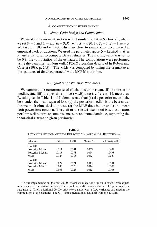
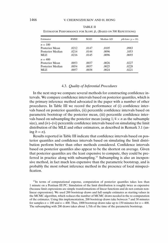
We compare the performance of (i) the posterior mean, (ii) the posteriormedian, and (iii) the posterior mode (MLE) across different risk measures.Results given in Tables I and II demonstrate that: (a) the posterior mean is thebest under the mean squared loss, (b) the posterior median is the best underthe mean absolute deviation loss, (c) the MLE does better under the mean10th power loss function. Thus, all of the listed likelihood-based estimatorsperform well relative to some risk measure and none dominate, supporting thetheoretical discussion given previously.

TABLE IESTIMATOR PERFORMANCE FOR INTERCEPT β0 (BASED ON 500 REPETITIONS)

Estimator RMSE MAD Median AD pth loss (p = 10)

n= 100Posterior Mean .0114 .0081 .0059 .0401Posterior Median .0115 .0078 .0054 .0433MLE .0127 .0088 .0063 .0369


14In our implementation, the first 20000 draws are made for a “burn-in stage,” with adjust-ments made to the variance of transition kernel every 200 draws in order to keep the rejectionrate near 5. Then, additional 20000 draws were made with a fixed variance, and used in thecomputation of the estimates. The C++ implementation is available from the authors.


TABLE II

ESTIMATOR PERFORMANCE FOR SLOPE β1 (BASED ON 500 REPETITIONS)

Estimator RMSE MAD Median AD pth loss (p = 10)



4.3. Quality of Inferential Procedures

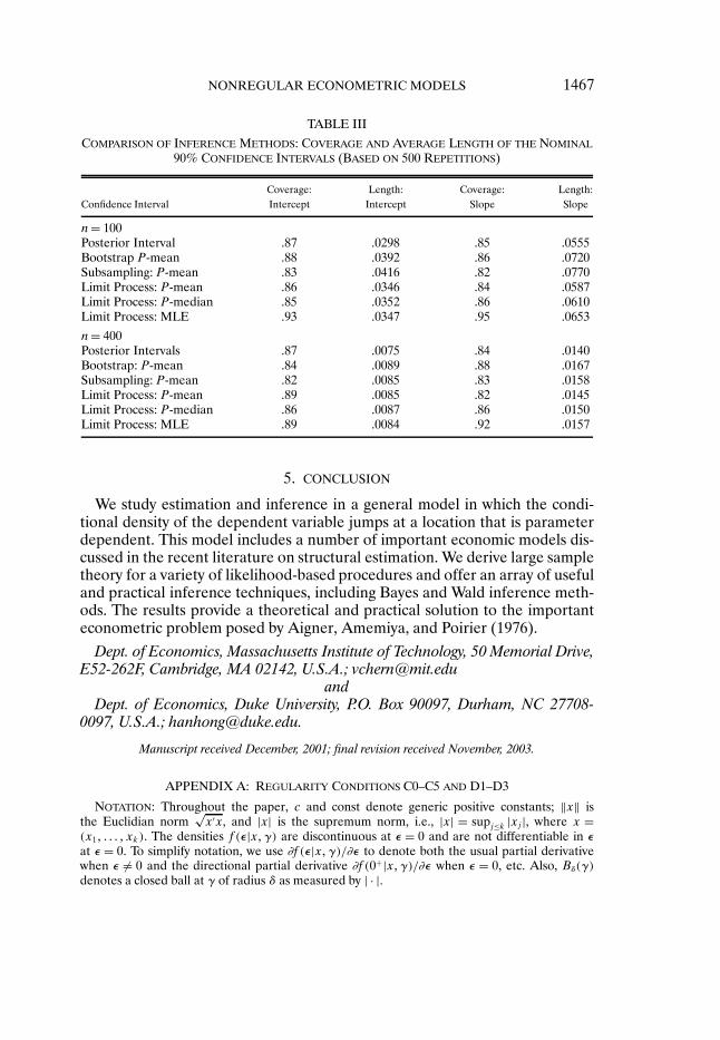
In the next step we compare several methods for constructing confidence in-tervals. We compare confidence intervals based on posterior quantiles, which isthe primary inference method advocated in the paper with a number of otherprocedures. In Table III we record the performance of (i) confidence inter-vals based on posterior quantiles, (ii) percentile confidence intervals based onparametric bootstrap of the posterior mean, (iii) percentile confidence inter-vals based on subsampling the posterior mean (using 1/4 ×n as the subsamplesize), and (iv)–(vi) percentile confidence intervals based on simulating the limitdistribution of the MLE and other estimators, as described in Remark 3.1 (us-ing b= n).

Results reported in Table III indicate that confidence intervals based on pos-terior quantiles and confidence intervals based on simulating the limit distri-bution perform better than other methods considered. Confidence intervalsbased on posterior quantiles also appear to be the shortest on average. Giventhat posterior quantiles are the least expensive to compute, they could be pre-ferred in practice along with subsampling.15 Subsampling is also an inexpen-sive method, in fact much less expensive than the parametric bootstrap, and isprobably the most robust inference method in the presence of local misspeci-fication.

15In terms of computational expense, computation of posterior quantiles takes less than1 minute on a Pentium III PC. Simulation of the limit distribution is roughly twice as expensive(because limit expressions are simple transformations of linear functions and do not contain non-linear expressions). We used 200 bootstrap draws and full sample estimates as starting values inthe MCMC algorithm, which reduces the number of MCMC draws needed in the re-computationof the estimates. Using this implementation, 200 bootstrap draws take between 7 and 30 minutesfor samples n = 100 and n = 400. Thus, 1000 bootstrap draws take up to 150 minutes for n= 400.The subsampling with 200 draws takes about 1/5th of the time of the parametric bootstrap.


TABLE III

COMPARISON OF INFERENCE METHODS: COVERAGE AND AVERAGE LENGTH OF THE NOMINAL90% CONFIDENCE INTERVALS (BASED ON 500 REPETITIONS)

Coverage: Length: Coverage: Length:Confidence Interval Intercept Intercept Slope Slope

n= 100Posterior Interval .87 .0298 .85 .0555Bootstrap P-mean .88 .0392 .86 .0720Subsampling: P-mean .83 .0416 .82 .0770Limit Process: P-mean .86 .0346 .84 .0587Limit Process: P-median .85 .0352 .86 .0610Limit Process: MLE .93 .0347 .95 .0653

n= 400Posterior Intervals .87 .0075 .84 .0140Bootstrap: P-mean .84 .0089 .88 .0167Subsampling: P-mean .82 .0085 .83 .0158Limit Process: P-mean .89 .0085 .82 .0145Limit Process: P-median .86 .0087 .86 .0150Limit Process: MLE .89 .0084 .92 .0157

5. CONCLUSION

We study estimation and inference in a general model in which the condi-tional density of the dependent variable jumps at a location that is parameterdependent. This model includes a number of important economic models dis-cussed in the recent literature on structural estimation. We derive large sampletheory for a variety of likelihood-based procedures and offer an array of usefuland practical inference techniques, including Bayes and Wald inference meth-ods. The results provide a theoretical and practical solution to the importanteconometric problem posed by Aigner, Amemiya, and Poirier (1976).

Dept. of Economics, Massachusetts Institute of Technology, 50 Memorial Drive,E52-262F, Cambridge, MA 02142, U.S.A.; [email protected]

andDept. of Economics, Duke University, P.O. Box 90097, Durham, NC 27708-

0097, U.S.A.; [email protected].

Manuscript received December, 2001; final revision received November, 2003.

APPENDIX A: REGULARITY CONDITIONS C0–C5 AND D1–D3

NOTATION: Throughout the paper, c and const denote generic positive constants; ‖x‖ isthe Euclidian norm

√x′x, and |x| is the supremum norm, i.e., |x| = supj≤k |xj |, where x =

(x1 xk). The densities f (ε|xγ) are discontinuous at ε = 0 and are not differentiable in εat ε = 0. To simplify notation, we use ∂f (ε|xγ)/∂ε to denote both the usual partial derivativewhen ε = 0 and the directional partial derivative ∂f (0+|xγ)/∂ε when ε = 0, etc. Also, Bδ(γ)denotes a closed ball at γ of radius δ as measured by | · |.


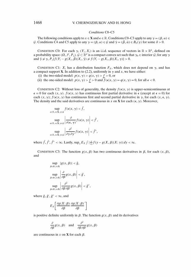
Conditions C0–C5

The following conditions apply to x ∈ X and ε ∈ R. Conditions C0–C3 apply to any γ = (βα) ∈G. Conditions C4 and C5 apply to any γ = (βα) ∈ G and γ = (β α) ∈ Bδ(γ) for some δ> 0.

CONDITION C0: For each γ, (YiXi) is an i.i.d. sequence of vectors in R × Rk, defined on

a probability space (ΩF Pγ). G ⊂ Rd is a compact convex set such that γ0 ∈ interior G; for any γ

and γ = γ, Pγf (Yi − g(Xi β)|Xi γ) = f (Yi − g(Xiβ)|Xiγ)> 0.

CONDITION C1: Xi has a distribution function FX , which does not depend on γ, and hasa compact support X. In addition to (2.2), uniformly in γ and x, we have either:

(i) the two-sided model: p(xγ) > q(xγ) > f > 0, or(ii) the one-sided model: p(xγ) > f > 0 and f (ε|xγ)= q(xγ) = 0, for all ε < 0

CONDITION C2: Without loss of generality, the density f (ε|xγ) is upper-semicontinuous atε = 0 for each (xγ). f (ε|xγ) has continuous first partial derivative in ε (except at ε = 0) foreach (xγ); f (ε|xγ) has continuous first and second partial derivative in γ, for each (x εγ).The density and the said derivatives are continuous in x on X for each (ε γ). Moreover,

supε∈Rx∈Xγ∈G

f (ε|xγ) < f


∣∣∣∣ ∂

∂(εγ)f (ε|xγ)

∣∣∣∣< f ′


∣∣∣∣ ∂2

∂γ ∂γ′ f (ε|xγ)∣∣∣∣< f ′′

where f , f ′, f ′′ < ∞. Lastly, supγ EX

∫ | ∂∂γf (y − g(Xβ)|X;γ)|dy < ∞

CONDITION C3: The function g(xβ) has two continuous derivatives in β, for each (xβ),and

supβ∈Bx∈X

|g(xβ)| < g

supβ∈Bx∈X

∣∣∣∣ ∂

∂βg(xβ)

∣∣∣∣ < g′

supβ∈Bx∈X

∣∣∣∣ ∂2

∂β∂β′ g(xβ)∣∣∣∣ < g′′

where g g′ g′′ < ∞, and

EX

[∂g(X;β)

∂β

∂g(X;β)∂β

′]is positive definite uniformly in β. The function g(xβ) and its derivatives

∂

∂βg(xβ) and

∂2

∂β∂β′ g(xβ)

are continuous in x on X for each β.


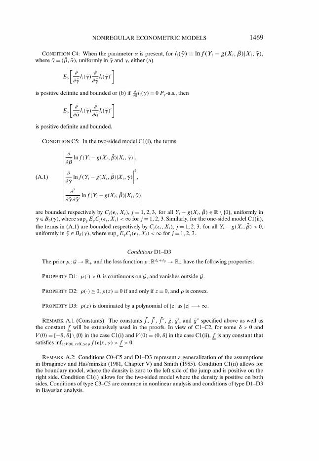
CONDITION C4: When the parameter α is present, for li(γ) ≡ ln f (Yi − g(Xi β)|Xi γ),where γ = (β α), uniformly in γ and γ, either (a)

Eγ

[∂

∂γli(γ)

∂

∂γli(γ)

′]

is positive definite and bounded or (b) if ∂∂βli(γ) = 0 Pγ-a.s., then

Eγ

[∂

∂αli(γ)

∂

∂αli(γ)

′]

is positive definite and bounded.

CONDITION C5: In the two-sided model C1(i), the terms∣∣∣∣ ∂

∂βln f (Yi − g(Xi β)|Xi γ)

∣∣∣∣∣∣∣∣ ∂

∂γln f (Yi − g(Xi β)|Xi γ)

∣∣∣∣2

(A.1) ∣∣∣∣ ∂2

∂γ ∂γ′ ln f (Yi − g(Xi β)|Xi γ)

∣∣∣∣are bounded respectively by Cj(εiXi), j = 123 for all Yi − g(Xi β) ∈ R \ 0, uniformly inγ ∈ Bδ(γ), where supγ EγCj(εiXi) < ∞ for j = 123. Similarly, for the one-sided model C1(ii),the terms in (A.1) are bounded respectively by Cj(εiXi), j = 123 for all Yi − g(Xi β) > 0,uniformly in γ ∈ Bδ(γ), where supγ EγCj(εiXi) < ∞ for j = 123.

Conditions D1–D3

The prior µ :G → R+ and the loss function ρ : Rdα+dβ → R+ have the following properties:

PROPERTY D1: µ(·) > 0, is continuous on G, and vanishes outside G.

PROPERTY D2: ρ(·) ≥ 0, ρ(z) = 0 if and only if z = 0, and ρ is convex.

PROPERTY D3: ρ(z) is dominated by a polynomial of |z| as |z| −→ ∞.

REMARK A.1 (Constants): The constants f , f ′, f ′′, g, g′ , and g′′ specified above as well asthe constant f will be extensively used in the proofs. In view of C1–C2, for some δ > 0 andV (0) = [−δδ] \ 0 in the case C1(i) and V (0) = (0 δ] in the case C1(ii), f is any constant thatsatisfies infε∈V (0)x∈Xγ∈G f (ε|xγ) > f > 0

REMARK A.2: Conditions C0–C5 and D1–D3 represent a generalization of the assumptionsin Ibragimov and Has’minskii (1981, Chapter V) and Smith (1985). Condition C1(ii) allows forthe boundary model, where the density is zero to the left side of the jump and is positive on theright side. Condition C1(i) allows for the two-sided model where the density is positive on bothsides. Conditions of type C3–C5 are common in nonlinear analysis and conditions of type D1–D3in Bayesian analysis.


APPENDIX B: PROOFS

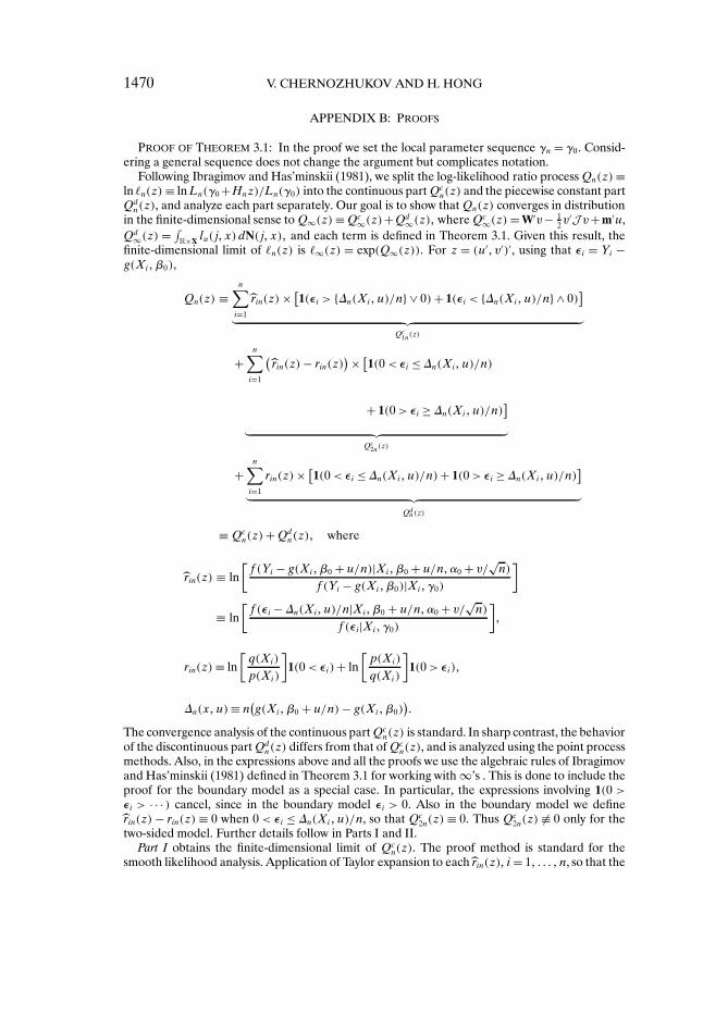
PROOF OF THEOREM 3.1: In the proof we set the local parameter sequence γn = γ0. Consid-ering a general sequence does not change the argument but complicates notation.

Following Ibragimov and Has’minskii (1981), we split the log-likelihood ratio process Qn(z) ≡ln n(z) ≡ lnLn(γ0 +Hnz)/Ln(γ0) into the continuous part Qc

n(z) and the piecewise constant partQd

n(z), and analyze each part separately. Our goal is to show that Qn(z) converges in distributionin the finite-dimensional sense to Q∞(z) ≡ Qc

∞(z)+Qd∞(z) where Qc

∞(z) = W′v− 12v

′J v+m′u,Qd

∞(z) = ∫R×X lu(j x)dN(j x) and each term is defined in Theorem 3.1. Given this result, the

finite-dimensional limit of n(z) is ∞(z) = exp(Q∞(z)) For z = (u′ v′)′ , using that εi = Yi −g(Xiβ0),

Qn(z) ≡n∑

i=1

rin(z) × [1(εi > ∆n(Xiu)/n ∨ 0)+ 1(εi < ∆n(Xiu)/n ∧ 0)

]︸︷︷︸

Qc1n(z)

+n∑

i=1

(rin(z)− rin(z)

) × [1(0 < εi ≤ ∆n(Xiu)/n)

+ 1(0 > εi ≥ ∆n(Xiu)/n)]

︸︷︷︸Qc

2n(z)

+n∑

i=1

rin(z)× [1(0 < εi ≤ ∆n(Xiu)/n)+ 1(0 > εi ≥ ∆n(Xiu)/n)

]︸︷︷︸

Qdn(z)

≡ Qcn(z)+Qd

n(z) where

rin(z) ≡ ln[f (Yi − g(Xiβ0 + u/n)|Xiβ0 + u/nα0 + v/

√n)

f (Yi − g(Xiβ0)|Xiγ0)

]

≡ ln[f (εi −∆n(Xiu)/n|Xiβ0 + u/nα0 + v/

√n)

f (εi|Xiγ0)

]

rin(z) ≡ ln[q(Xi)

p(Xi)

]1(0 < εi)+ ln

[p(Xi)

q(Xi)

]1(0 > εi)

∆n(xu)≡ n(g(Xiβ0 + u/n)− g(Xiβ0)

)

The convergence analysis of the continuous part Qcn(z) is standard. In sharp contrast, the behavior

of the discontinuous part Qdn(z) differs from that of Qc

n(z), and is analyzed using the point processmethods. Also, in the expressions above and all the proofs we use the algebraic rules of Ibragimovand Has’minskii (1981) defined in Theorem 3.1 for working with ∞’s . This is done to include theproof for the boundary model as a special case. In particular, the expressions involving 1(0 >εi > · · ·) cancel, since in the boundary model εi > 0. Also in the boundary model we definerin(z) − rin(z) ≡ 0 when 0 < εi ≤ ∆n(Xiu)/n, so that Qc

2n(z) ≡ 0 Thus Qc2n(z) ≡ 0 only for the

two-sided model. Further details follow in Parts I and II.Part I obtains the finite-dimensional limit of Qc

n(z). The proof method is standard for thesmooth likelihood analysis. Application of Taylor expansion to each rin(z), i = 1 n, so that the


expanded terms are i.i.d., followed by application of the Markov LLN and Chebyshev inequality,yields for a given z

Qc1n(z) ≡ −u′E∆(Xi)

f ′(εi|Xγ0)

f (εi|Xiγ0)︸︷︷︸≡u′m

+v′[

1√n

n∑i=1

∂

∂αlnf (εi|Xiγ0)

]︸︷︷︸

≡Wn

+ 12v′

[E

∂2

∂α∂α′ log f (ε|Xγ0)

]︸︷︷︸

≡−J

v + op(1)

where ∆(Xi) = ∂g(Xiβ0)/∂β. The information matrix equality for α implies

−J = E∂2 log f (ε|Xγ0)

∂α∂α′

= −E∂ log f (ε|Xγ0)

∂α

∂ log f (ε|Xγ0)

∂α

′

and the CLT gives Wnd→ W = N (0J ) Also, it follows by C2 that m = E∆(Xi)(p(Xi)− q(Xi))

Therefore, the finite-dimensional limit of Qc1n(z) is given by Qc

∞(z) ≡ u′m + W′v − 12v

′J vIt remains to show Qc

2n(z) = op(1). In the one-sided case Qc2n(z) ≡ 0; hence we only need to

consider the two-sided case. Note that by C1–C3, for any compact set Z, as n → ∞, for someconstant c that depends only on f /f and g′ ,∣∣∣∣ ln

[f (ε−∆n(xu)/n|xβ0 + u/nα0 + v/

√n)

f (ε|xγ0)

]− ln

[q(x)

p(x)

]∣∣∣∣(B.1)

≤ c × ‖z‖/√n

uniformly in ε z x ∈ R+ × Z × X :∆n(xu) > 00 < ε≤ ∆n(xu)/n. Likewise∣∣∣∣ ln[f (ε−∆n(xu)/n|xβ0 + u/nα0 + v/

√n)

f (ε|xγ0)

]− ln

[p(x)

q(x)

]∣∣∣∣(B.2)

≤ c × ‖z‖/√n

uniformly in ε z x ∈ R− × Z × X :∆n(xu) < 00 > ε≥ ∆n(xu)/n. Thus

supz∈Z

|Qc2n(z)| ≤ c × ‖Z‖/√n×

n∑i=1

1(|εi| <K/n)= Op(1/√n)(B.3)

for K= ‖Z‖ × g′ < ∞, where ‖Z‖ = sup‖z‖ :z ∈ Z, where K < ∞ by C3. The Op(1/√n) con-

clusion is by C2:

E

n∑i=1

1(|εi| <K/n) ≤ 2fK < ∞(B.4)

Part II obtains the finite-dimensional limit of Qdn(z). Recall

Qdn(z) ≡

n∑i=1

[ln

q(Xi)

p(Xi)1(0 <nεi ≤ ∆n(Xiu))+ ln

p(Xi)

q(Xi)1(0 > nεi ≥ ∆n(Xiu))

]


By C2 and C3

E

n∑i=1

∣∣1(0 <nεi ≤ ∆n(Xiu))− 1(0 <nεi ≤ ∆(Xi)

′u)∣∣

+ ∣∣1(0 > nεi ≥ ∆n(Xiu))− 1(0 > nεi ≥ ∆(Xi)

′u)∣∣

≤ 2f g′′‖u‖2/n = o(1)

where ∆(Xi) ≡ ∂g(Xiβ0)/∂β, which implies that for a given z

Qdn(z) =

n∑i=1

[ln

q(Xi)

p(Xi)1(0 < nεi < ∆(Xi)

′u) + ln

p(Xi)

q(Xi)1(0 > nεi > ∆(Xi)

′u)]

+ op(1)

Now note that (Qdn(zj) j ≤ l) and (Qc

n(zj) j ≤ l), for any finite l, are asymptotically inde-pendent. This follows by applying a standard argument concerning the independence of extremeorder statistics and sample averages; see, e.g., Lemma 21.19 in van der Vaart (1999). Details areomitted for brevity, but can be found in Chernozhukov and Hong (2001a).

The next step is to obtain the finite-dimensional limit of Qdn . The behavior of Qd

n is determinedby near-to-jump observations, which behavior is described using point processes. We split theargument in two steps. Step 1 constructs the required point process and derives its limit. Step 2applies Step 1 to obtain the finite-dimensional limit of Qd

n .Step 1. The intuition for Step 1 is provided in Section 3.2 of the main text.Define E ≡ R × X. The topology on E is standard; e.g., [ab] × X is a compact subset relative

to E. The point process of interest is a random measure taking the following form: for any Borelsubset A, N(A) = ∑n

i=1 1[(nεiXi) ∈ A] We take N to be a random element of Mp(E), themetric space of nonnegative point measures on E, with the metric generated by the topology ofvague convergence; cf. Resnick (1987, Chapter 3). We show that N ⇒ N in Mp(E) for N given inTheorem 3.1. This is done in the steps (a) and (b).

(a) By C1 and C2, for any F ∈ T , the basis of relatively compact open sets in E (finite unionsand intersections of open bounded rectangles in E),

limn→∞

EN(F) ≡ limn→∞

nP((nεiXi) ∈ F

)=

∫F

[p(x)1(u > 0)du+ q(x)1(u < 0)du]dFX(x)(B.5)

= m(F) <∞

where the measure m is defined as dm(ux) = [p(x)1(u > 0)du + q(x)1(u < 0)du]dFX(x)Since (nεiXi) ∈ F are independent across i by C0, by Meyer’s Theorem (cf. Meyer (1973))

limn→∞P(N(F) = 0) = e−m(F)(B.6)

Statements (B.5) and (B.6) imply by Kallenberg’s theorem (cf. Resnick (1987, Proposition 3.22))that N ⇒N in Mp(E), where N is a Poisson point process with the mean intensity measure m(·).

(b) Next we show that N has the same distribution as N given in Theorem 3.1. First, con-sider the canonical Poisson processes N0 and N ′

0 with points Γi and Γ ′i defined in Theo-

rem 3.1. N0 has the mean measure m0(du) = du on (0∞), and N ′0 has the mean measure

m′0(du) = du on (−∞0); see Resnick (1987, p. 138). Because N0 and N ′

0 are independent,N1(·) ≡ N0(·) + N0(·)′ is a Poisson point process with mean measure m1(du) = du on R bydefinition of the Poisson process; see Resnick (1987, p. 130). Because XiX ′

i are i.i.d. andindependent of Γi Γ

′i , by Proposition 3.8 in Resnick (1987), the composed process N2 with

points (ΓiXi Γ ′i X ′

i i≥ 1) is a Poisson process with the mean measure m2(dudx) = [1(u >


0)du+ 1(u < 0)du]×FX(dx) on R × X Finally, N with the points T(ΓiXi) T (Γ ′i X ′

i ), whereT : (ux) → (1(u > 0)u/p(x) + 1(u < 0)u/q(x)x), is a Poisson process with the desired meanmeasure m(dudx) = m2 T−1(dudx) = [p(x)1(u > 0) + q(x)1(u < 0)]duFX(dx) by Propo-sition 3.7 in Resnick (1987).

Step 2. We have for z = (u′ v′)′,

Qdn(z) = Qd

n(u) =[

n∑i=1

lnq(Xi)

p(Xi)1[0 < nεi ≤ ∆(Xi)

′u]

+n∑

i=1

lnp(Xi)

q(Xi)1[0 >nεi ≥ ∆(Xi)

′u]]

+ op(1)

Ignoring the op(1) term, write Qdn(u) as a Lebesgue integral with respect to N:

Qdn(u)=

∫E

lu(j x)dN(j x)

where lu(j x) is defined in Theorem 3.1. The convergence of this integral is implied by N ⇒ N inboth the two-sided and one-sided model:

(a) In the two-sided model: By conditions C1–C3, the function (j x) → lu(j x) is boundedand vanishes outside the compact set Ku ≡ [−η+η] × X, η = supx∈X |∆(x)′u|, where η < ∞by C3. Thus (j x) → lu(j x) has compact support but is discontinuous when j = 0 and j = ∆(x)′u.Define the map T :Mp(E) → R

l as N → (∫Eluk(j x)dN(j x)k≤ l) for l < ∞. Hence by Propo-

sition 3.13 in Resnick (1987), T is discontinuous at D(T )≡ N ∈Mp(E) : jNi = 0 or jNi = u′k∆(x

Ni )

for some i ≥ 1 k ≤ l where (jNi xNi i≥ 1) denote the points of N . Since εi’s are absolutely con-

tinuous, P[N ∈ D(T ), for some n ≥ 1] = 0, and by definition of N, P[N ∈ D(T )] = 0 ThereforeN ⇒ N in Mp(E) implies T(N)

d→ T(N) by the continuous mapping theorem; cf. Resnick (1987,p. 153). It follows that (Qd

n(uk)k ≤ l)d→ (Qd

∞(uk)k ≤ l) where Qd∞(u) ≡ ∫

Elu(j x)dN(j x)

(b) In the one-sided model: Using the Ibragimov and Has’minskii (1981) rules for algebraicoperations with ∞’s stated in Theorem 3.1, note that Qd

n(u) = ∫Elu(j x)dN(j x) is a binomial

random variable: Qdn(u) = −∞ if N(A(u)) > 0 and Qd

n(u) = 0 if N(A(u)) = 0 where A(u) ≡(j x) ∈ R+ × X : j ≤ ∆(x)′u Also define Qd

∞(u) ≡ ∫Elu(j x)dN(j x), so that Qd

∞(u) = −∞if N(A(u)) > 0 and Qd

∞(u) ≡ 0 if N(A(u)) = 0 Thus, to show the finite-dimensional conver-gence (for γk = −∞ or 0): limn→∞ P(Qd

n(uk) = γkk≤ l)= P(Qd∞(uk) = γkk≤ l) it suffices to

show (N(A(uk))k ≤ l)d→ (N(A(uk))k ≤ l) for l < ∞. By a definition of weak convergence of

point processes (cf. Embrechts, Klüppelberg, and Mikosch (1997, p. 232)), this is immediate fromN ⇒ N, since by C2 and construction of N, N(∂A(uk)) = 0 and N(∂A(uk)) = 0 a.s. Q.E.D.

PROOF OF THEOREM 3.2: The proof applies Theorem I.10.2 of Ibragimov and Has’minskii(1981, p. 107), which allows one to obtain the limit distribution of BEs provided some conditionson the likelihood ratio process are satisfied.

First, BEs are measurable by the Jennrich’s measurability theorem since they minimize ob-jective functions that are continuous in data and parameters. Second, we shall make use of thefollowing important lemmas proved in Appendix C. Let γ = (βα) and h = (hβhα). Define theHellinger distance

r2(γ;γ + h)2

=∫ ∫ ∣∣f 1/2

(y − g(xβ+ hβ);xγ + h

) − f 1/2(y − g(xβ);xγ)∣∣2

dyFX(dx)

Note that F1/2X (dx) is taken outside the | · |2-brackets, since it does not depend on the parameters.


LEMMA B.1 (Hellinger distance properties): Under C0–C5, there are a > 0 and A> 0 such thatfor all h such that γ + h ∈ G, uniformly in γ ∈ G

(a) r22(γ;γ + h) ≥ 2

amax(|hβ| |hα|2)1 + max(|hβ| |hα|2) and(B.7)

(b) r22(γ;γ + h) ≤ A(|hβ| + |hα|2)

LEMMA B.2 (Exponential tails and Holder continuity): Given (B.7), for all n > n0, (z z′) withγ +Hnz ∈ G and γ +Hnz

′ ∈ G, and some a′ > 0 and n0, uniformly in γ ∈ G

Eγ n(z)1/2 ≤ e−a′(|z|−1) Eγ| n(z)1/2 − n(z

′)1/2|2 ≤ A(|z − z′|)(1 + 2 · |z′| ∨ |z|)(B.8)

The following conditions 1–4 verify the conditions of Theorem I.10.2 of Ibragimov andHas’minskii (1981, p. 107):

1. Holder continuity of 1/2n (z) in the mean square, and the exponential bound on the expected

likelihood tail, both proved in Lemma B.2. In the latter case, we have that for a′ > 0, Eγ n(z)1/2 ≤

e−a′(|z|−1) where z → a′(|z|−1) falls into the function class G of Ibragimov and Has’minskii (1981,p. 41), i.e., a′(|z| − 1) is increasing in |z| on [0∞) and lim|z|→∞ |z|Ne−a′(|z|−1) = 0 for any N > 0.

2. Finite-dimensional convergence of n(z) = exp(Qn(z)) to ∞(z) = exp(Q∞(z)), establishedin Theorem 3.1.

3. The limit Bayes problem,

Z = arg infz′∈Rd

∫Rd

ρ(z′ − z) ∞(z)∫

Rd ∞(z)dzdz

is uniquely solved by a random vector Z, which is by D2 (since ρ is convex with a unique minimum;cf. Ibragimov and Has’minskii (1981, p. 107)).

4. Conditions D1–D3 on the loss functions ρ and prior µ. (It must be noted that Ibragimov andHas’minskii (1981) impose the symmetry of ρ throughout their book. However, the inspectionof their proof of Theorems I.10.2 (and Theorem I.5.2) reveals that the proof does not requiresymmetry and applies to the loss functions that satisfy D1–D3.)

Thus, conditions 1–4 imply by Theorem I.10.2 of Ibragimov and Has’minskii (1981) that Znd→

Z Furthermore, conditions 1–4 imply by Theorem I.5.2 and Theorem I.10.2 of Ibragimov andHas’minskii (1981) that for any δ ∈ R

d , γnδ = γ0 +Hnδ, N > 0,

limL→∞n→∞

L−NPγnδ |Zn| >L = 0 and limn→∞

Eγnδρ(Zn) =Eγ0ρ(Z) <∞(B.9)

The result (B.9) is not needed to prove Theorem 3.2 but will be used later. Q.E.D.

PROOF OF THEOREM 3.3: To show Claim 1, note that limn→∞ Eγnδ [H−1n (γ − γn)] = Eγ0 Z

by (B.9). Consider the problem minc Eγ0ρ(Z+ c), where ρ(z) = z′z. The solution of this problemis c = −EZ. Suppose that c = 0; then

Eγ0ρ(Z + c) < Eγ0ρ(Z)(B.10)

where by Lemma 3.1 stated in Section 3.5 the left-hand side of (B.10) is the asymptotic averagerisk of the sequence of estimators γ + Hnc and the right-hand side of (B.10) is the asymptoticaverage risk of the sequence of posterior means γ, which contradicts the asymptotic average riskefficiency of the posterior mean established in Lemma 3.1. Thus it must be that c = −EZ = 0.

To show Claim 2, note that by Theorem 3.2 and the definition of weak convergence,

limn→∞Pγnδ (γ(τ))j ≤ (γ0)j = lim

n→∞Pγnδ(Zn(τ))j ≤ 0 = Pγ0 (Z(τ))j ≤ 0since 0 is assumed to be a continuity point of the distribution of (Z(τ))j . Consider theproblem minc Eγ0ρ((Z(τ))j − c;τ) where ρ(z;τ) = (1(z ≥ 0) − τ)z. Note that the quantity


Eγ0ρ((Z(τ))j − c;τ) is finite for any c by (B.9). A solution of this problem is given by the root ofthe first-order condition

Pγ0(Z(τ))j ≥ c = τ or Pγ0 (Z(τ))j ≤ c = 1 − τ(B.11)

i.e., c = (1 − τ)th quantile of (Z(τ))j (under the condition that (Z(τ))j has positive density inany small neighborhood of 0). Suppose c = 0; then

Eγ0ρ((Z(τ))j − c;τ)<Eγ0ρ

((Z(τ))j;τ

)(B.12)

where by Lemma 3.1 the left-hand side of (B.12) is the asymptotic average risk of the sequenceof estimators defined as (γ(τ) −Hnc)j , and the right-hand side is the asymptotic average risk ofthe posterior τth quantile (γ(τ))j . See Section 3.5 and Lemma 3.1 for definitions. Then (B.12)contradicts the asymptotic average risk efficiency of the posterior quantiles under the check lossfunction established in Lemma 3.1.

Thus it must be that c = 0 in (B.11), so that the first part of Claim 2, (3.10), is proven. Thesecond part of Claim 2, (3.11), is immediate from (B.11) with c = 0 for τ = τ′ and τ = τ′′:

limn→∞Pγnδ (γ(τ′))j ≤ (γn(δ))j ≤ (γ(τ′′))j(B.13)

= limn→∞

Pγnδ (Zn(τ′))j ≤ 0 ≤ (Zn(τ

′′))j= 1 − lim

n→∞Pγnδ (Zn(τ′′))j ≤ 0 − lim

n→∞Pγnδ (Zn(τ′))j ≥ 0

= 1 − Pγ0 (Z(τ′′))j ≤ 0 − Pγ0 (Z(τ′))j ≥ 0 = τ′′ − τ′ Q.E.D.

PROOF OF THEOREM 3.4: We will use the following lemma.

LEMMA B.3 (Integral convergence of n(z)): Suppose that (i) n(z) has the properties specifiedin Lemma B.2 and (ii) n(z) converges marginally to ∞(z) under a parameter sequence γnδ =γ0 + Hnδ. Then (a) ∞(z) > 0 in some open ball at zero a.s., (b) for any vector-valued continuousfunction g(z) dominated by a polynomial as z → ∞∫

Kn

g(z) n(z)µ(γ0 +Hnz)∫

Kn n(z′)µ(γ0 +Hnz′)dz′ dz

d→∫K

g(z) ∞(z)∫

K ∞(z′)dz′ dz

Here either Kn = Un ≡ z :γnδ + Hnz ∈ G and K = Rd or Kn = K = U , where U is a fixed cube

centered at the origin; andd→ denotes weak convergence under Pγn .

The first part of the proof of Theorem 3.4 is done by setting the true parameter sequenceγnδ = γ0. Considering a general sequence does not change the argument but complicates nota-tion. Write Zn(τ) = (c(τ) − rn(γ0)). Note that Zn(τ) ≡ arg infz∈R

Γn(z), where

Γn(z)≡∫

Rd

ρ(z − rn(γ0 +Hnz)+ rn(γ0);τ

) n(z)µ(γ0 +Hnz)∫Rd n(z′)µ(γ0 +Hnz′)dz′ dz

Since |rn(γ0 +Hnz)−rn(γ0)−R′z| ≤ const |z| · |Hnz|a′ for a′ > 0, by the piece-wise linearity of thecheck function we have that |ρ(z− rn(γ0 +Hnz)+ rn(γ0);τ)−ρ(z−R′z;τ)| ≤ const · |z| · |Hnz|a′ .Hence by Lemma B.3

Γn(z) =∫

Rd

(ρ(z −R′z;τ)+O(|z| · |Hnz|a′

)) n(z)µ(γ0 +Hnz)∫

Rd n(z′)µ(γ0 +Hnz′)dz′ dz(B.14)

=∫

Rd

ρ(z −R′z;τ) n(z)µ(γ0 +Hnz)∫Rd n(z′)µ(γ0 +Hnz′)dz′ dz + op(1)


Applying Lemma B.3 again, it follows that the marginal limit of Γn(z) is given by

Γ∞(z) =∫

Rd

ρ(z −R′z;τ) ∞(z)∫Rd ∞(z′)dz′ dz

Recall that Z(τ) denotes the minimizer of Γ∞(z). By the Convexity Lemma, e.g., Knight (2000)and Davis, Knight, and Liu (1992), the stated finite-dimensional convergence of convex objectivefunctions implies Zn(τ)

d→ Z(τ) Thus, in what follows it suffices to consider only linear functionssuch that rn(γ0 +Hnz)− rn(γ0)−R′z = 0 for all z.

Next, we need to establish the uniform integrability of ρ(Zn(τ);τ). Consider the linear trans-formation ξ = M ′z defined by a nonsingular matrix M such that R is a column of M . Then, thelikelihood for ξ given by n(M

−1ξ) satisfies for some c > 0 and c′ > 0:

(a) Eγ| 1/2n (M−1ξ′)− 1/2

n (M−1ξ′′)|2 ≤ c|ξ′ − ξ′′|(1 + 2|ξ′| ∨ |ξ′′|)(b) Eγ

1/2n (M−1ξ) ≤ e−c′(|ξ|−1)

by nonsingularity of M and Lemma B.2. By Theorem I.5.2 of Ibragimov and Has’minskii (1981)for any local sequence of γnδ = γ0 +Hnδδ ∈ R

d , and any N > 0, limL→∞n→∞ L−NPγnδ|Zn(τ)| >L = 0. Hence limn→∞ Eγnδρ(Zn(τ);τ) = Eγ0ρ(Z(τ);τ) < ∞ Then similarly to Lemma 3.1, itcan be concluded that c(τ) minimizes the asymptotic average risk, i.e., it achieves the infimumof

lim supK↑Rd

lim supn→∞

1λ(K)

∫K

Eγnδρ(Zn;τ)dδ

over all statistic sequences c that are measurable functions of (YiXi i ≤ n), where Zn =c − rn(γnδ). The rest of the argument, which establishes the (1 − τ)-quantile unbiasedness ofthe posterior τ-quantiles and the resulting coverage properties, is identical to the proof of Theo-rem 3.3. Q.E.D.

PROOF OF LEMMA 3.1: Claim 1 is just a special case of Theorem 1.1 of Lehmann and Casella(1998, Chapter 5). Claim 2 follows by the argument given by Ibragimov and Has’minskii (1981,p. 93). Details can be found in Chernozhukov and Hong (2001a). Q.E.D.

APPENDIX C: PROOFS OF LEMMAS B.1–B.4

PROOF OF LEMMA B.1: In order to establish (B.7)(b), let γ = (βα) and h = (hβhα),

r22(γ;γ + h)

= EX

∫ (f 1/2(y − g(Xβ + hβ)|X;β+ hβα+ hα)− f 1/2(y − g(Xβ)|X;γ))2

dy

(1)≤ EX

∫[g(Xβ)g(Xβ+hβ)]

∣∣f (y − g(Xβ + hβ)|X;β+ hβα+ hα)

− f (y − g(Xβ)|X;γ)∣∣dy+EX

∫[g(Xβ)g(Xβ+hβ)]c

(f 1/2(y − g(Xβ+ hβ)|X;γ + h)

− f 1/2(y − g(Xβ+ hβ)|X;β+ hβα))2dy

+EX


∣∣f (y − g(Xβ+ hβ)|X;β+ hβα)

− f (y − g(Xβ)|X;γ)∣∣dy


(2)≤ 2EX |g(Xβ+ hβ)− g(Xβ)|f

+ const |hα|2∫ 1

0EX

∫ ∣∣∣∣∂f 1/2(y − g(Xβ+ hβ)|Xβ+ hβα+ωhα)

∂α

∣∣∣∣2

dy dω

+ const |hβ|∫ 1

0EX

∫ ∣∣∣∣∂f (y − g(Xβ+ωhβ)|Xβ+ωhβα)

∂β

∣∣∣∣dy dω(3)≤ const f |hβ|EX

∫ 1

0

∣∣∣∣∂g(Xβ +ωhβ)

∂β

∣∣∣∣dω+ const (|hα|2)+ const (|hβ|)

(4)= const (|hβ|)+ const (|hα|2)where [ab] = [ab] if a ≤ b and = [ba] if b ≤ a, and the bound is uniform in γ. (1) is bytriangle inequality and |a− b|2 ≤ |a2 − b2| for a > 0 and b > 0. The first term in (2) follows from|f (·|·)| ≤ f . The second and third terms in (2) are by Taylor expansion and Fubini. The first termin (3) follows from Taylor expansion and Fubini. The second term in (3) follows from C4, whilethe third term in (3) is by C2. (4) is by C3.

The lower bound from below, equation (B.7)(a), is established by considering separately|h| ≤ δ for some sufficiently small δ and |h| > δ. Indeed, for sufficiently small δ and |h| ≤ δ itis shown below that

r22(γ;γ + h) ≥ const max(|hβ| |hα|2)(C.1)

On the other hand, by the identification condition C0 for all |h| > δ such that γ + h ∈ G,

r22(γ;γ + h) ≥ εδ > 0(C.2)

Hence for some a > 0 the bound in (B.7)(a) is immediate from (C.1)–(C.2).It remains to prove (C.1) for |h| < δ for some sufficiently small δ. Write

r22(γ;γ + h) = EX

∫[g(Xβ)g(Xβ+hβ)]

(f 1/2(y − g(Xβ+ hβ)|X;γ + h)

− f 1/2(y − g(Xβ)|X;γ))2dy︸︷︷︸

I

+EX


(f 1/2(y − g(Xβ+ hβ)|X;γ + h)

− f 1/2(y − g(Xβ)|X;γ))2dy︸︷︷︸

II

For small hβ, we can bound I from below uniformly in γ by

EX

12|g(Xβ+ hβ)− g(Xβ)||p1/2(Xγ)− q1/2(Xγ)|2

≥ constEX

∣∣∣∣∂g(X;β)∂β

′hβ

∣∣∣∣ ≥ const |hβ|

using C3 and Taylor expansion. On the other hand, by C1–C3, bound II from below by

EX


(h′ ∂f

1/2(y − g(X;β)|γ)∂γ

)2

dy − o(|h|2)


By C2, C3, and C4(a), a further lower bound on II is

|h|2 inf|u|=1

EX


(f 1/2(y − g(Xβ);γ)

∂γ

′u

)2

dy

≥ |h|2(

inf|u|=1

EX

∫ (∂f 1/2(y − g(Xβ);γ)

∂γ

′u

)2

dy +O(|hβ|))

≥ const |h|2 ≥ const |hα|2for all sufficiently small |h|, where the remainder term O(|hβ|) arises from neglecting the inte-grand over the small area [g(Xβ) g(Xβ + hβ)] and using the bounds in C2 and C3 to do so.On the other hand, if assumption C4(b) holds, the uniform lower bound on II is

EX

∫ (h′ ∂f

1/2(y − g(X;β)|γ)∂γ

)2

dy

≥ const |hα|2 inf|u|=1

EX

∫ (f 1/2(y − g(Xβ);γ)

∂α

′u

)2

dy

≥ const |hα|2for all sufficiently small |h|. Conclude infγ r2

2 (γ;γ + h) ≥ const max(|hβ| |h2α|). Q.E.D.

PROOF OF LEMMA B.2: We have

Eγ n(z)1/2 (1)≤

[1 − 1

2r2

2(γ;β+ u/nα+ v/√n)

]n

(2)≤ exp−n

2r2

2(γ;β+ u/nα+ v/√n)

(3)≤ exp

−a

max(|u| |v|2)1 + max(|u| |v|2)/n

(4)≤ exp

−a

max(|u| |v|2)1 +KG

(5)≤ exp

−a|z| + a

1 +KG

where the constant KG depends only on the diameter of the parameter space G; (1) follows by thestandard manipulation of the Hellinger distance, as in Ibragimov and Has’minskii (1981, p. 260);(2) follows by the inequality (1 − r) ≤ e−r when r > 0; (3) is given by (B.7), and (4) and (5) areobvious. Also,

Eγ| n(z)1/2 − n(z′)1/2|2 (1)≤ nr2

2

(γ + (u/n v/

√n);γ + (u′/n v′/

√n)

)(2)≤ A(|u− u′| + |v − v′|2)(3)≤ A(|z − z′| + |z − z′|2)(4)≤ A(|z − z′|)(1 + 2 · |z′| ∨ |z|)


where (1) follows by the standard manipulation of the Hellinger distance, as in Ibragimov andHas’minskii (1981, p. 260), (2) is given, and (3) and (4) are obvious. Q.E.D.

PROOF OF LEMMA B.3: Assertion (a) is a special case of Lemma I.5.1 in Ibragimov andHas’minskii (1981). Assertion (b) is proven of Ibragimov and Has’minskii (1981, pp. 106–109)under more general conditions than conditions (i) and (ii). Q.E.D.

REFERENCES

AIGNER, D., T. AMEMIYA, AND D. POIRIER (1976): “On the Estimation of Production Frontiers:Maximum Likelihood Estimation of the Parameters of a Discontinuous Density Function,”International Economic Review, 17, 377–396.

BOWLUS, A., G. NEUMANN, AND A. KIEFER (2001): “Equilibrium Search Models and the Tran-sition from School to Work,” International Economic Review, 42, 317–343.

CHERNOZHUKOV, V. (2000): “Conditional Extremes and Near-Extremes: Estimation, Inference,and Economic Applications,” Ph.D. Dissertation, Department of Economics, Stanford.

CHERNOZHUKOV, V., AND H. HONG (2001a): “Likelihood Inference in a Class of Nonregu-lar Econometrics Models,” MIT Department of Economics Working Paper, Revised October2003, distributed by the Social Science Research Network, http://www.ssrn.com.

(2001b): “Likelihood Inference with Density Jumps,” MIT Department of EconomicsWorking Paper, presented at CEME Conference.

CHRISTENSEN, B., AND A. N. KIEFER (1991): “The Exact Likelihood Function for an EmpiricalJob Search Model,” Econometric Theory, 7, 464–486.

DAVIS, R. A., K. KNIGHT, AND J. LIU (1992): “M-estimation for Autoregressions with InfiniteVariance,” Stochastic Processes and Applications, 40, 145–180.

DONALD, S. G., AND H. J. PAARSCH (1993a): “Maximum Likelihood Estimation when the Sup-port of the Distribution Depends upon Some or All of the Unknown Parameters,” WorkingPaper, Department of Economics, University of Western Ontario.

(1993b): “Piecewise Pseudo-Maximum Likelihood Estimation in Empirical Models ofAuctions,” International Economic Review, 34, 121–148.

(1996): “Identification, Estimation, and Testing in Parametric Empirical Models of Auc-tions Within Independent Private Values Paradigm,” Econometric Theory, 12, 517–567.

(2002): “Superconsistent Estimation and Inference in Structural Econometric ModelsUsing Extreme Order Statistics,” Journal of Econometrics, 109, 305–340.

EMBRECHTS, P., C. KLÜPPELBERG, AND T. MIKOSCH (1997): Modelling Extremal Events. Berlin:Springer-Verlag.

FLINN, C., AND J. HECKMAN (1982): “New Methods for Analyzing Structural Models of LaborForce Dynamics,” Journal of Econometrics, 18, 115–190.

GHOSAL, S. (1999): “Probability Matching Priors for Non-Regular Cases,” Biometrika, 86,956–964.

GHOSAL, S., AND T. SAMANTA (1995): “Asymptotic Behaviour of Bayes Estimates and Poste-rior Distributions in Multiparameter Nonregular Cases,” Mathematical Methods of Statistics, 4,361–388.

HIRANO, K., AND J. PORTER (2003): “Asymptotic Efficiency in Parametric Structural Models withParameter-Dependent Support,” Econometrica, 71, 1307–1338.

IBRAGIMOV, I., AND R. HAS’MINSKII (1981): Statistical Estimation: Asymptotic Theory. New York:Springer-Verlag.

KNIGHT, K. (2000): “Epi-convergence and Stochastic Equisemicontinuity,” Working Paper, Uni-versity of Toronto.

(2002): “Limiting Distributions of Linear Programming Estimators,” Extremes, 4, 87–103.KOENKER, R., AND G. S. BASSETT (1978): “Regression Quantiles,” Econometrica, 46, 33–50.LEHMANN, E., AND G. CASELLA (1998): Theory of Point Estimation. New York: Springer-Verlag.


MEYER, R. M. (1973): “A Poisson-Type Limit Theorem for Mixing Sequences of Dependent RareEvents,” The Annals of Probability, 1, 480–483.

PAARSCH, H. (1992): “Deciding Between the Common and Private Value Paradigms in EmpiricalModels of Auctions,” Journal of Econometrics, 51, 191–215.

POLITIS, D., J. ROMANO, AND M. WOLF (1999): Subsampling. New York: Springer-Verlag.PORTNOY, S., AND J. JURECKOVÁ (2000): “On Extreme Regression Quantiles,” Extremes, 2,

227–243.RESNICK, S. I. (1986): “Point Processes, Regular Variation and Weak Convergence,” Advances in

Applied Probability, 18, 66–138.(1987): Extreme Values, Regular Variation, and Point Processes. New York: Springer-

Verlag.ROBERT, C. P., AND G. CASELLA (1998): Monte Carlo Statistical Methods. New York: Springer-

Verlag.SMITH, R. L. (1985): “Maximum Likelihood Estimation in a Class of Nonregular Cases,” Bio-

metrika, 72, 67–90.(1994): “Nonregular Regression,” Biometrika, 81, 173–183.

TIERNEY, L. (1994): “Markov Chains for Exploring Posterior Distributions,” The Annals of Sta-tistics, 22, 1701–1762.

VAN DER VAART, A. (1999): Asymptotic Statistics. New York: Cambridge University Press.(2000): “Lectures on Bayesian Statistics,” Unpublished Manuscript, Aarhus University.

WALD, A. (1950): Statistical Decision Functions. New York: John Wiley & Sons.

Documents

Econometrica, Vol. 72, No. 5 (September, 2004), 1445–1480vchern/papers/ch_density_jump.pdf · Econometrica, Vol. 72, No. 5 (September, 2004), 1445–1480 LIKELIHOOD ESTIMATION AND