Regulation Initiative Discussion Paper Series Number 44

ECONOMETRIC COST FUNCTIONS

Melvyn A. Fuss University of Toronto

Leonard Waverman

London Business School

Chapter 5 in Cave, Majumdar and Vogelsang (eds) Handbook of Telecommunications Economics, Kluwer, forthcoming

2

Contents 1. Introduction

1.1. Monopoly or Competition 1.2. Regulation and Price-Caps: The Need for Assessing Productivity

1.3. Efficiency Examination and the Use of Alternative Approaches 1.4. General Comments

2. The Concepts of Economies of Scale, Economies of Scope and Subadditivity 2.1 Economies of Scale and Scope

3. Technological Change 3.1. Estimating Marginal Costs 3.2. Revenue Weights versus Cost Weights in Price-Caps Formulae

4. A Review of the Evidence 4.1. Recent Results on Scale Economies in Other Segments

5. Conclusion References

1. INTRODUCTION The knowledge of costs is crucial in any industry, and has proven to be of special importance in telecommunications. The telecommunications industry has long been organized in most jurisdictions as a monopoly regulated by the state. Hence, the firm has had the knowledge of its costs, yet the state and the regulator have needed to regulate prices and to determine where entry, if any, should be allowed. The telecommunications carrier provides multiple services over a certain geographic area using capital that is fixed and common across a variety of applications. In addition, the impact of technological advance is also unevenly spread over the range of assets and services. Hence, a determination of costs, especially at an individual service level, is inherently difficult. Moreover, since the carrier, the regulator and the entrants have had different objectives, the information publicly available has always been limited. Academic economists have played important roles in the public policy process, and econometric cost functions were used more in this industry than in any other context.

As competition has grown, the debates concerning the presence or absence of natural monopoly elements in telecommunications have gradually subsided. The importance of public knowledge of firm-specific costs has not, however, correspondingly decreased. Where entrants compete with incumbents that originally were the sole providers of network services, the issues of the price (cost) to interconnect at, and of the wholesale price of ‘unbundled’ services have become crucial. Therefore, issues of ‘correct social costs’ have not diminished. What were, in the 1970’s and 1980’s, questions of natural monopoly, sustainable prices and unsustainable cross-subsidies have become questions of access pricing and entry conditions.

In this paper, we survey the uses and abuses of econometric cost function analysis in the telecommunications sector. Simultaneously, in the past decade, applications of accounting based techniques1 and operations research based techniques2 to study performance and the nature of production in the telecommunications sector have steadily increased. We do not survey these techniques in detail. We briefly highlight the role of operations research based techniques, but restrict ourselves to a more extensive discussion of econometric based techniques in this survey. Detailed and extensive reviews of the accounting and operations research based literatures are left as future agenda items.

1.1. Monopoly or Competition A hotly contested issue in the 1970’s and 1980’s, and in the early 1990’s was whether competition in the provision of various services, public long distance or message toll (toll) services, local services and even in terminal equipment in the customer’s home or office, was in the public interest. Incumbent telephone companies consistently argued that the provision of each and every one of these services was a natural monopoly. Hence, a competitive market structure was inefficient. On the other hand, in recent years, many nations, such as the United States in 1977, Japan in 1985, the United Kingdom in 1986, New Zealand in 1990, South Korea

1 See Banker, Chang and Majumdar (1996) and Fraquelli and Vanoni (2000). 2 See Majumdar (1995) and Uri (2001).

in 1991, Canada in 1993, and the countries of the European Union in 1998, have introduced competition.

Economists have been a consistent part of the debate, and a large number of empirical papers utilising econometric cost functions have led, followed and often criticised competition. The influential initial findings of Fuss and Waverman (1981a, 1981b), Fuss (1983), and Evans and Heckman (1983, 1984, 1986, 1988) were that competition in toll services was feasible. A number of other authors have concluded that competitive toll provision is inefficient (Charnes, Cooper and Sueyoshi (1988), Gentzoglanis and Cairns (1989), Pulley and Braunstein (1990), Röller (1990a,b), Ngo (1990), Diewert and Wales (1991a,b). Other authors have, more recently, used a variety of techniques to examine the costs of the provision of local services (Shin and Ying, 1992; Gabel and Kennet, 1994; Majumdar and Chang, 1998). These authors have reached conflicting conclusions concerning the desirability of competition in the provision of local services. Shin and Ying (1992) and Majumdar and Chang (1998) broadly support local competition, while Gabel and Kennett (1994) and Wilson and Zhou (2001) take the opposite view. In this survey we evaluate this conflicting evidence at both the toll and local service levels, and investigate the extent to which it is relevant to the kinds of changes in the market structure of the telecommunications industry, which have been made.

1.2. Regulation and Price-Caps: The Need for Assessing Productivity Cost functions are also used for other important issues in telecommunications. They have proved important in establishing the form of regulation. First they were used to show the inefficiency of rate-of-return regulation. Now they are used to determine the crucial x factor. This is the rate of productivity improvement in price-caps proceedings.3 Economies of scale and scope, allocative efficiency, and technical advance (productivity improvement) are all parts of the same puzzle. Therefore, determining efficiency or relative efficiency and the ‘x’ factor requires disentangling all the impacts of cost changes – scale, scope, innovation, regulation and factor price changes.

It is this disentanglement that is inherently difficult. The developers of the growth accounting literature (Denison, 1985; Solow, 1957; Jorgenson and Griliches, 1967), to name but a few, did not consider the problems associated with applying their methodology to an industry characterized by a high proportion of fixed and common costs, rapid technical change, and overt and changing government regulation.

A simple example indicates the nature of the problem: Total factor productivity growth (TFP ) is traditionally measured as the difference

between Divisia indices of aggregate measures output and input growth (Diewert, 1976). TFP is the ratio of aggregate output Y to aggregate input X, so that:

PFTο

= Yο

- (1) ο

X and

3 The conceptual and empirical issues relating to price-cap regulation are covered by Sappington in the

chapter of ‘Price Regulation’ in this Handbook, and we do not go into details of this topic.

ο

Y =ο

jj

jj YRYP

.∑ (2)

where =jP of price of output j

jY = quantity of output j

jYο

= proportionate rate of growth of output jR = = total revenue j

jjYP∑

and ο

X =ο

ii

ii XCXw

⋅∑ (3)

where =iw price of output i

iX = quantity of output i

iXο

= proportionate rate of growth of output i , and C = i

ii Xw∑ = total cost.

The aggregate production function takes the form

oF (Y1, .Ym ; ; t ) = 0 (4) nXX ..1

where is the production function and t = a technical advance indicator, or oF C = G ( ; Ynww ..................1 1,…… .Ym ; ) (5) t

where G (..) is the cost function. Totally differentiating (5) and re-arranging yields,

- =ο

B jj

CY Yj

−∑ε -

ο

ii

ii XCXw

⋅∑ (6)

where

- = technical change (the proportionate shift in the cost function with time), and ο

B

jCYε = cost elasticity of the output. thj

If production is characterised by constant returns to scale and all individual outputs are priced in the same proportion relative to marginal cost, ε = pjCY jYj / R and ∑ ε = 1. jCY

Then: - =ο

B Yο

- (7) ο

X

Or - = T (7a). ο

B PFο

However, with increasing returns to scale (decreasing returns to costs) Denny Fuss and Waverman (1981) have demonstrated that measured TFP growth (or the factor) consists both of true technical change plus returns to increased scale. The relevant formula is

'' x

PFTο

= - + (1- Σε ) ο

BjCY

ο

Y

(7b). Therefore, to estimate TFP growth requires estimates of ε and hence knowledge of the cost function. We return to the issues of measuring technical change and the ‘x’ factor in section (3) below.

jCY

One issue is very important to raise here in this introduction. In the parametric analysis of production structure, the choice of the functional form of the cost function has proven to be crucial. The majority of the analyses utilize a variant of the transcedental logarithmic (translog) cost function. The translog function is a second order approximation to an unknown cost function that imposes a minimal number of prior constraints on the specification of the underlying technology. This fact, and the additional fact that the estimating equations that result from applying the translog functional form are linear in parameters, has made it a popular function. However, a number of studies (Fuss, 1983; Röller, 1992) identify problems with the translog function as a flexible approximation. These problems can lead to biased estimates of economies of scale and scope (and the productivity factor) if the true underlying cost function is poorly approximated by the translog function over the range of data that is of interest.

'' x

One possible solution is to estimate a functional form that contains the translog function as a special case (for example, the Box-Cox function [see Fuss, 1983]). But this does not avoid the functional form issue. Another solution is to search for methods that do not rely on a chosen functional form as being the correct representation of the true unknown technology. A functional form is not imposed on the data. Rather, the data are left to ‘speak’ for themselves. Hence, the use of procedures which are non-parametric.4 These techniques however raise other problems – namely the robustness of the estimation and their underlying statistical properties.

1.3. Efficiency Measurement and the Use of Alternative Approaches A third general area of analysis has been the examination of the efficiency of the operations of specific firms. This is feasible with the use of goal programming and the allied Data Envelopment Analysis (DEA) techniques.5 These belong to a family of non-parametric estimation methods useful for evaluating production conditions. Our emphasis in this chapter

4 Non-parametric techniques such as DEA (Data Envelopment Analysis) makes no assumption about

functional form other than convexity and piece-wise linearity. This property is extremely useful since functional relations between various inputs and outputs can be very difficult to define, if the assumptions of causal ambiguity and heterogeneity at the firm level (Lippman and Rumelt, 1982) are made.

5 See Banker, Charnes and Cooper (1984) and Charnes, Cooper and Rhodes (1978) for details of the primary algorithms.

is on econometric techniques, per-se. Thus, we only briefly describe DEA and other non-parametric techniques.6

As far as we are aware, Charnes, Cooper and Sueyoshi (1986) were the first to utilize non-parametric techniques in the estimation of cost functions for the telecommunications sector. Rather than using some form of average curve fitting of a specific functional form, using ordinary least squares (OLS) or maximum likelihood estimation (MLE) techniques, they utilized goal-programming/constrained regression techniques to examine the nature of subadditivity in the Bell SystemBell System.

Since then, the use of DEA for efficiency analysis has been done with primarily two purposes in mind. First, to determine whether regulated firms were on the least cost expansion path (Majumdar, 1995). Second, to benchmark various dimensions of performance and production characteristics (Majumdar and Chang, 1996). DEA is a procedure that fits a curve to the outside (convex hull) of the data points. It is one of a class of techniques that define the maximal outputs for given levels of inputs.7 The firm (s) at the outside envelope are defined as efficient; those with lower output for identical levels of inputs are relatively “inefficient.”

Following Majumdar (1995) Identify as weights on output and input , which we calculate to maximize

the efficiency rating of the firm.ir vu , ry ix

kh thk 8

),( vuhk = ∑

∑

=

=m

iiki

s

rrkr

xv

yu

1

1 (8)

The derived linear mathematical programming problem is:

ν,µ

max kw = (9) ∑=

s

rrkr y

1µ

subject to

∑=

m

iiki x

1

ν = 1

6 See Seiford (1996) and Seiford and Thrall (1990) for more extensive reviews of the DEA literature. 7 Another technique in this class is the frontier cost or production function technique. An important

difference between DEA analysis and frontier cost function estimation is that the former is a non-parametric technique, whereas the latter is a method of estimating the parameters of a specific function. However, DEA can be used with multiple outputs, while the use of the frontier cost or production functions is restricted to the single output case. See Jha and Majumdar (1999) for an application of parametric frontier cost estimation techniques in the analysis of telecommunications sector issues.

8 Other constraints are incorporated so that each efficiency ratio < 1.

∑=

s

rrjr y

1

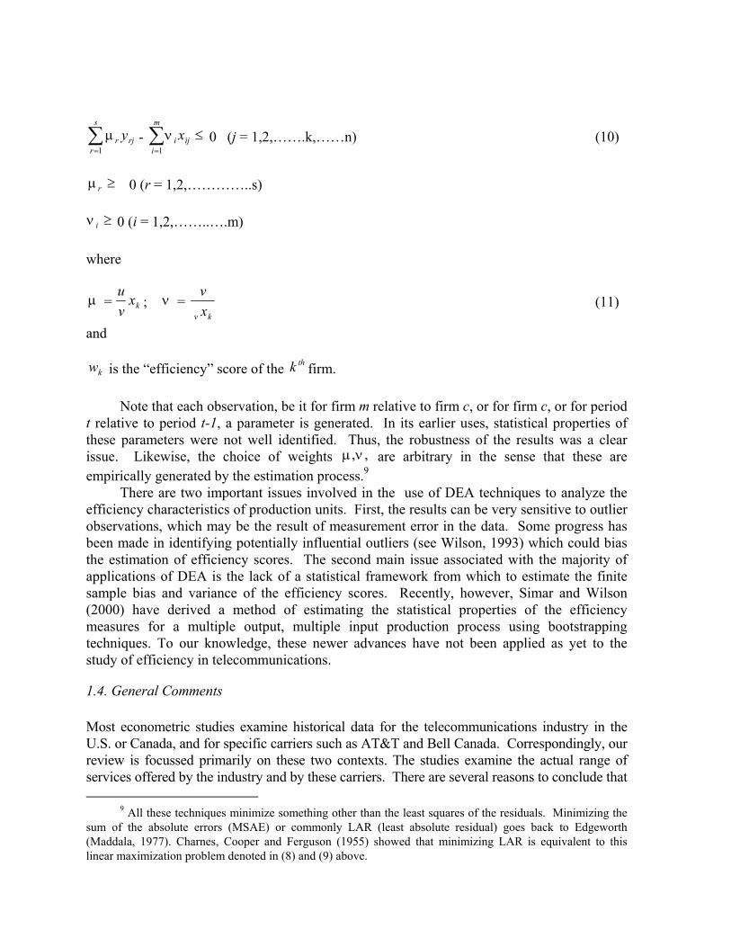
µ - ∑ 0 (j = 1,2,…….k,……n) (10) ≤=

m

iiji x

1

ν

≥rµ 0 (r = 1,2,…………..s)

≥iν 0 (i = 1,2,……..….m)

where

µ = kxvu

; ν = kv x

v (11)

and

kw is the “efficiency” score of the firm. thk

Note that each observation, be it for firm m relative to firm c, or for firm c, or for period t relative to period t-1, a parameter is generated. In its earlier uses, statistical properties of these parameters were not well identified. Thus, the robustness of the results was a clear issue. Likewise, the choice of weights are arbitrary in the sense that these are empirically generated by the estimation process.

,,νµ9

There are two important issues involved in the use of DEA techniques to analyze the efficiency characteristics of production units. First, the results can be very sensitive to outlier observations, which may be the result of measurement error in the data. Some progress has been made in identifying potentially influential outliers (see Wilson, 1993) which could bias the estimation of efficiency scores. The second main issue associated with the majority of applications of DEA is the lack of a statistical framework from which to estimate the finite sample bias and variance of the efficiency scores. Recently, however, Simar and Wilson (2000) have derived a method of estimating the statistical properties of the efficiency measures for a multiple output, multiple input production process using bootstrapping techniques. To our knowledge, these newer advances have not been applied as yet to the study of efficiency in telecommunications.

1.4. General Comments Most econometric studies examine historical data for the telecommunications industry in the U.S. or Canada, and for specific carriers such as AT&T and Bell Canada. Correspondingly, our review is focussed primarily on these two contexts. The studies examine the actual range of services offered by the industry and by these carriers. There are several reasons to conclude that

9 All these techniques minimize something other than the least squares of the residuals. Minimizing the sum of the absolute errors (MSAE) or commonly LAR (least absolute residual) goes back to Edgeworth (Maddala, 1977). Charnes, Cooper and Ferguson (1955) showed that minimizing LAR is equivalent to this linear maximization problem denoted in (8) and (9) above.

cost function analyses were not robust for the initial public policy purposes of the 1970’s and 1980’s, which was to determine the socially correct degree of entry into each service or across services or even the ‘divestiture’ of AT&T itself. First, the US and Canadian industries were organised as regional monopolies until recently. AT&T provided about 80 percent of the U.S. telecommunications services until 1984. Bell Canada had a legal monopoly over most of Quebec and Ontario provinces until 1992. Hence, the data that the econometrics relied on were for a firm that provided a set of services and existed as a regulated monopoly with strict entry barriers.

Second, there were few carriers who provided single services. Thus, the one empirical result consistent across most studies, including early ones, is the existence of economies of scale in the provision of telecommunications services in the aggregate. This provides no indication as to whether or not individual services such as toll or local service should be monopolised or not. Third, the econometric results that conceptually could provide such evidence, those pertaining to toll-specific economies of scale and existence of natural monopoly (established by the subadditivity of the cost function), do not withstand careful scrutiny.

In order to specify tests of service-specific economies of scale and subadditivity relevant to the question at hand, the researcher must be able to estimate the technology of a firm that produces only that service. Little actual data exist in any country, with the exception of very recent post-entry data, which pertain to such a ‘stand-alone’ firm. In any case, such data have rarely been used in econometric estimations of the telecommunications production technology.

This lack of appropriate data has forced researchers into one of two straightjackets. The first has been to concentrate on analyses that are not relevant to the emerging market structures. These are generally characterised by a multi-product firm facing a firm, or firms, which provide only toll service and are interconnected with the multi-product firm which provides both local as well as toll services. The second has led to an incorrect specification of the cost function, which represented the stand-alone technology, and to the projection of the estimated function far outside the actual experiences of the firms whose data sets were used for estimation.

2. THE CONCEPTS OF ECONOMIES OF SCALE, SCOPE, AND SUBADDITIVITY This section describes the econometric approaches to evaluating cost and production functions. We discuss the concepts of economies of scale, economies of scope, and subadditivity. These are concepts central to an understanding of the econometrics literature.

2.1. Economies of Scale and Scope Before proceeding to a more detailed discussion of the actual econometric studies, it is useful to provide a brief outline of the concepts of economies of scale, economies of scope, and subadditivity, concentrating on the applicability of these concepts to the question of the desirability of competition in the provision of a single telecommunications service. Due to the intense interest in this and other public policy questions that require knowledge of the telecommunications production technology, several extensive reviews of the econometrics literature have been published (see especially Fuss, 1983; Kiss and Lefebvre, 1987; and Waverman, 1989). Each of these studies provides a detailed description of the concepts of scale,

scope and subadditivity as they have been used in the econometrics literature. Here to simplify the discussion we concentrate on their applicability to the first main question addressed - the competitive provision of toll services.

These concepts can most easily be understood in terms of a firm's cost function. This is the function that is almost always estimated in contemporary analyses of the telecommunications production technology. The cost function of a telecommunications firm is defined as the firm's minimum cost of providing a set of telecommunications services, conditional on given purchase prices of the factors of production and on a particular state of technology (see equation 5). In this section we simplify the mathematical presentation by deleting these conditioning variables from explicit consideration. Also for simplicity we will restrict ourselves to the case where only two outputs are produced: toll service (YT) and local service (YL). For a firm that produces both toll and local services, the cost function takes the form C = C(YT,YL) (12). For a firm which produces only toll services, CT = CT(YT) (13) and for a firm which produces only local services, CL = CL(YL) (14). Note that by superscripting C in equations (13) and (14) we have specified, as seems reasonable, that firms which produce only toll services or only local services have production technologies that differ from the production technology of a firm which produces toll and local services jointly. This difference is sufficiently fundamental that these technologies cannot be recovered from equation (12) simply by setting the missing output equal to zero. This observation is very important since it means that (13) or (14) can never be recovered from data generated by a firm represented by (12). Unfortunately, the assumption that (13) or (14) can be recovered from (12) is maintained in all the econometrics literature which considers this issue explicitly.

When will the specifications of (12), (13) and (14) be appropriate, and the specification used in the econometrics literature incorrect? One situation in which this will occur for most forms of the cost function is if there are fixed costs in the provision of services, but these fixed costs differ depending on whether the firm supplies toll, or local, or both. Another situation arises if the value of marginal cost depends on whether the firm corresponds to (12), (13), or (14).

One can illustrate the preceding argument by specifying three very simple cost functions for C, CT, and CL. Suppose the joint production technology, toll-only technology, and local-only technology cost functions take the forms:10

10 We ignore technical change in this section for simplicity.

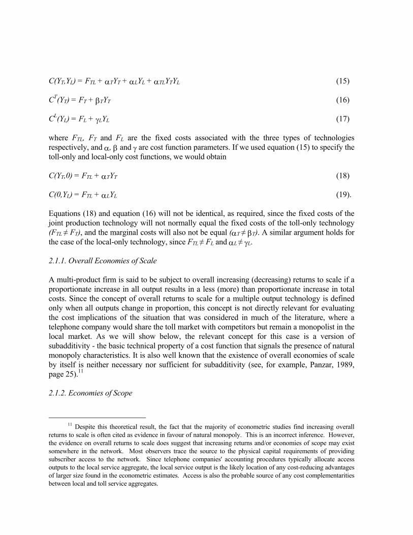
C(YT,YL) = FTL + αTYT + αLYL + αTLYTYL (15) CT(YT) = FT + βTYT (16) CL(YL) = FL + γLYL (17) where FTL, FT and FL are the fixed costs associated with the three types of technologies respectively, and α, β and γ are cost function parameters. If we used equation (15) to specify the toll-only and local-only cost functions, we would obtain C(YT,0) = FTL + αTYT (18) C(0,YL) = FTL + αLYL (19). Equations (18) and equation (16) will not be identical, as required, since the fixed costs of the joint production technology will not normally equal the fixed costs of the toll-only technology (FTL ≠ FT), and the marginal costs will also not be equal (αT ≠ βT). A similar argument holds for the case of the local-only technology, since FTL ≠ FL and αL ≠ γL. 2.1.1. Overall Economies of Scale A multi-product firm is said to be subject to overall increasing (decreasing) returns to scale if a proportionate increase in all output results in a less (more) than proportionate increase in total costs. Since the concept of overall returns to scale for a multiple output technology is defined only when all outputs change in proportion, this concept is not directly relevant for evaluating the cost implications of the situation that was considered in much of the literature, where a telephone company would share the toll market with competitors but remain a monopolist in the local market. As we will show below, the relevant concept for this case is a version of subadditivity - the basic technical property of a cost function that signals the presence of natural monopoly characteristics. It is also well known that the existence of overall economies of scale by itself is neither necessary nor sufficient for subadditivity (see, for example, Panzar, 1989, page 25).11 2.1.2. Economies of Scope

11 Despite this theoretical result, the fact that the majority of econometric studies find increasing overall

returns to scale is often cited as evidence in favour of natural monopoly. This is an incorrect inference. However, the evidence on overall returns to scale does suggest that increasing returns and/or economies of scope may exist somewhere in the network. Most observers trace the source to the physical capital requirements of providing subscriber access to the network. Since telephone companies' accounting procedures typically allocate access outputs to the local service aggregate, the local service output is the likely location of any cost-reducing advantages of larger size found in the econometric estimates. Access is also the probable source of any cost complementarities between local and toll service aggregates.

The second concept of interest is that of economies of scope. A firm which produces both toll and local services is said to enjoy economies of scope if it can produce these services at lower cost than would occur if each service were produced separately by a stand-alone firm. We can measure economies of scope by the variable SCOPE, where SCOPE = [CT(YT) + CL(YL) - C(YT,YL)] / C(YT,YL) (20) If we multiply SCOPE by 100, it measures the percentage change in total cost of stand-alone productions of toll and local services compared with the cost of joint production of the two services by a single firm. If SCOPE > 0 economies of scope exist, whereas if SCOPE<0 diseconomies of scope exist. The above ideas can be illustrated using our simple cost functions (15), (16) and (17). If we substitute these functions into equation (20), the numerator of (20) becomes: NUM = (FT+FL-FTL) + (αT-βT)YT + (αL-γL)YL - αTLYTYL (21). SCOPE is greater than zero when NUM is greater than zero. NUM will more likely be greater than zero when joint production yields savings in total fixed costs (FTL<FT+FL), and when joint production yields cost complementarities (αTL<0). The signs of the other terms in (21) depend on the marginal cost relationships among the joint and stand-alone technologies, and could plausibly be either positive or negative. Although equation (21) corresponds to the definition of SCOPE given by equation (20) for our simple cost functions, it does not correspond to what would be calculated in the econometrics literature. First, all studies in the econometrics literature which attempt to measure economies of scope assume that FTL=FT=FL, so that all the fixed costs associated with the provision of both toll and local services would be borne by each stand-alone firm. This clearly overstates the fixed cost contribution to a positive SCOPE, since it assumes that having separate toll and local service-providing firms will necessarily lead to complete duplication of facilities. It is more likely that some facilities will be jointly used. For example, when Mercury Communications entered the toll market in the United Kingdom, it did not construct its own local loops but shared British Telecom's local service facilities through interconnection. Second, the econometric studies normally implicitly assume that the second and third terms in (14) are identically equal to zero, since there would be no provision for the possibility of distinct stand-alone technologies.

There is a third issue that is illustrated by our simple cost functions. The presence of the cost complementarity term αTLYTYL in NUM implies that estimates of SCOPE using (13) will be calculated under the assumption that the entirety of any cost complementarity that may exist would be lost if the provisions of toll and local services were separated. This assumption is another source of overestimation of possible lost economies of scope, since interconnection of facilities would substantially mitigate this effect.

The above discussion illustrates the importance of interconnection provisions and the proper pricing of these provisions, when competition with an incumbent telecommunications operator is permitted, in order that any network economies of scope that may be present not be

lost. 2.1.3. Product-Specific Returns to Scale The third concept that is of interest is the concept of product-specific returns to scale. Suppose we measure the incremental cost of producing toll services for a firm that already produces local services as: ICT = C(YT,YL) - CL(YL) (22) Then toll-specific returns to scale is measured by ST = ICT /(YT.MCT) (23) where MCT is the marginal cost of supplying toll services when the firm produces both toll and local services. If ST>1 the firm is said to produce toll services with increasing returns to scale, if ST<1 toll-specific returns to scale are said to be decreasing, and if ST=1 toll-specific returns to scale are said to be constant. Similarly, local-specific returns to scale is measured by SL = [C(YT,YL) - CT(YT)] /(YL.MCL) (24) There is an interesting and illuminating relationship between overall returns to scale, product-specific returns to scale, and economies of scope given by the equation (see for example Panzar [1989]): S = [aT.ST + aL.SL] /(1-SCOPE) (25) where aT = (YT.MCT)/(YT.MCT+YL.MCL) and aL = (YL.MCL)/(YT.MCT+YL.MCL) are cost elasticity shares for toll and local services respectively, and S is the measure of overall returns to scale.

From equation (25) we can see why a finding of increasing overall returns to scale tells us nothing of relevance for the question of whether competition should be allowed in the provision of toll services. There are numerous combinations of product- specific returns to scale and returns to scope characteristics that could result in increasing overall returns to scale.12 2.1.4. Subadditivity The fourth concept of interest is that of subadditivity. This is the concept most closely

12 One situation which would unambiguously favour competition in the provision of toll services is the

scenario where ST<1 (toll-specific diseconomies of scale), SCOPE=0 (absence of economies of scope) and SL>1 (local-specific economies of scale). If local- specific economies of scale are large and toll-specific diseconomies of scale are small, this configuration would likely produce a finding of overall economies of scale (S>1).

connected to the question of whether a firm is a natural monopolist in the provision of the services demanded in the marketplace. Hence, it is most directly relevant to the issue of competitive provision of toll services. A telephone company will be a natural monopolist in the provision of toll and local services if it can provide the levels of services demanded at lower cost than can be provided if alternative sources of supplies are permitted. This must be true for all possible levels of services. In this case, we say that the cost function of the monopolist is subadditive. For the situation of one versus two firms found in the econometrics literature, we can measure the degree of subadditivity from the equation (see Evans and Heckman [1983]): SUB = {C(YT,YL) - [C(φ.YT,ω.YL) + C((1-φ).YT+(1-ω).YL)]} / C(YT,YL) (26) When SUB is multiplied by 100, it measures the percentage difference in total industry costs between single firm production of toll and local services and any two firm configuration. The particular two firm configuration is determined by the weights φ and ω which designate the way in which industry output is divided between the two firms. If SUB<0 for all possible values of φ and ω the industry cost function is subadditive and single firm production is cost-minimizing. The condition is stringent. If any values of φ and ω can be found for which SUB>0, monopoly provision of both toll and local services is not cost-minimizing.

The test of subadditivity based on equation (26) is a global test, and is both necessary and sufficient for the existence of a natural monopoly. However, this test requires that the cost function be valid for values of outputs well outside the range of actual experience, including stand-alone production of both toll and local services (e.g. when φ=1 and ω=0 or φ=0 and ω=1). It also requires that when only one output is produced by a firm, CT(YT)=C(YT,0) and CL(YL)=C(0,YL). This, as noted previously, is unlikely to be correct.

To counteract the criticism associated with the global test, i.e., that the cost function must be valid for outputs outside the range of actual experience, Evans and Heckman (EH) developed a local test of subadditivity, in which they restricted φ and ω to values such that neither of the two firms in the competitive scenario would produce outside of the historically-observed range of the monopolist. The EH test has been used in all subsequent tests of natural monopoly (except Röller [1990a] and Pulley and Braunstein [1990]). However the EH test is only a necessary test, and because it is not sufficient, can only be used to reject the existence of natural monopoly, not confirm it.13

Aside from the limited nature of the evidence that the EH test generally provides, it has an important flaw in the present circumstances. The data region in which one firm provides both toll and local services, and other firms provide only toll services is outside the data region used to estimate telecommunications cost functions. Thus the EH test is undefined for the case of competitive entry normally under consideration and results based on this test were not relevant to the kinds of competitive entry taking place around the world in the 1980’s and 1990’s.14

13 In the words of Evans and Heckman (1983, p. 36): “Our test is one of necessary conditions for natural

monopoly. Rejection of that hypothesis is informative. Acceptance within a region ... is not informative. All that acceptance demonstrates is that there are inefficient ways to break up AT&T. Failure to reject the necessary conditions for natural monopoly does not imply that AT&T was a natural monopoly....To perform such a test requires extrapolation of the cost function well outside the range of the data used to estimate it.”

14 The EH test was developed in conjunction with the anti-trust litigation which led to the divestiture of

A variant of the subadditivity test is relevant for the type of competitive entry that is being analyzed. Suppose we replace equation (16) with an alternative definition of SUB, denoted SUBT:

SUBT = {C(YT,YL) - [CT(φ.YT) + C((1-φ).YT,φ.YT,YL)]} / C(YT,YL) (27). Comparing (27) with (26) we see that there are three differences. First, in (27) ω=0 (one firm produces no local output). Second, the cost function for producing toll output alone has a superscript T to indicate, as noted previously, the different nature of the toll stand-alone technology. Third, the toll output of the stand-alone firm enters the cost function of the other firm as an economies of scope cost-reducing externality, since, as also noted previously, the two firms will be interconnected and hence share facilities such as terminal equipment and local loops. This sharing of facilities will mitigate cost increases that are associated with a loss of economies of scope. These will be suffered by the joint output-producing firm via the diversion of toll output to the other firm. Of course the cost function for the toll-only producing firm will have to include any interconnection costs which are caused specifically by the entry of the competitor.

If SUBT<0 for all values of φ such that 0<φ<1, then single firm production is cost-minimizing, otherwise competitive provision of toll services does not raise supply costs. This is the correct subadditivity (or natural monopoly) test for the version of competitive entry that is relevant outside of the U.S. (see footnote 8). Unfortunately, SUBT has never been calculated. This is perhaps not surprising since the calculation requires knowledge of the toll stand-alone technology and the economies of scope effect of interconnection. Only Röller (1990a) performs a global test as is required. However, the use of his results to compute SUBT would bias the test towards a finding of subadditivity for two reasons. First, he assumes the amount of fixed costs would be the same for a toll stand-alone technology as they are estimated to be for the monopoly firm supplying both toll and local services. Second, Röller's model implies all economies of scope associated with the toll-only firm's output would be lost if two firms operated in the toll market while one firm supplied all the local output, contrary to the reality of interconnected facilities.

The calculation of SUBT would provide the correct static test of the natural monopoly hypothesis, but even this calculation would fail to take into account the dynamic effects of competitive entry on the costs of service provision. In particular, there are three effects, which imply that the correct static test is itself biased in favour of a finding of natural monopoly when the dynamic setting is ignored. First, the static test assumes the level of total demand is the same pre- and post-competition. To the extent that competition-induced market stimulation leads to expanded markets, and there exist economies of scale and scope, both the incumbent and entrant's unit costs will be overstated by the static test. Second, competition will likely act as a spur to increased efficiency on the part of the incumbent, or a reduction in x-inefficiency

AT&T. It was designed to analyze a market structure in which competing toll-producing firms would interconnect with local-producing firms that would not be in the inter-state toll provision business. This kind of market structure is unique to the United States. In other countries, the market structure analyzed in this paper, where toll-producing firms compete with a firm (the former monopolist) that produces both toll and local services and provides facilities for interconnection, is the relevant market structure.

(Majumdar, 1995), and for this reason the incumbent's post-entry costs are overstated by the static test. Finally, the static test assumes the same state of technology pre- and post-competition. To the extent that technical change in the industry is accelerated by the presence of competition, the static test overstates the post-competition costs of both the incumbent and entrant firms.

On the other side of the ledger, the static test does not consider any inter-temporal costs associated with competition, such as the potential ongoing interconnection costs and increased marketing costs that are specific to the existence of a competitor. 3. TECHNOLOGICAL CHANGE15 As noted in the introduction, the analysis of technological change has been crucial in telecommunications as cost reductions come about through changes in factor prices or technical change. Thus, looking at technical change issues in a formal way is useful. Technical advances have been a hallmark of the telecommunications sector, since the sector relies on both switching equipment, using computers and semi-conductors, and transmission equipment using radio and multiplexing. Technological change has affected various services differently. Hence, the possibility of efficient entry in separate service markets was affected by technical progress. With the replacement of rate-of-return regulation with price-caps regulation, the measurement of technical progress (the expected productivity enhancement) is a crucial aspect of the regulatory regime, and econometric measurement of technical progress is a part of the process.

The conventional Törnqvist index16 for measuring TFP growth between years t-1 and t is calculated from the log difference formula:

∆ log TFPR = ∆ log YR – ∆ log X (28) where ∆ log YR = Σ (1/2) (Rjt + Rj,t-1).[log Yjt - log Yj,t-1] (29) ∆ log X = Σ (1/2)(Sit + Si,t-1).[log Xit - log Xi,t-1] (30) where Yjt is the amount of the ith output produced at time t, Xit is the amount of the ith input utilized at time t, Rjt is the revenue share of the ith output in total revenue, and

15 This section draws heavily from Fuss (1994). 16 The Törnqvist index is a discrete time empirical approximation to the continuous Divisia index

introduced earlier.

Sit is the cost share of the ith input in total cost. The superscript R indicates that revenue weights are used in the calculations. ∆ log Y and ∆ log X are often referred to as the rates of change of aggregate output and aggregate input respectively, since they result from procedures which aggregate the rates of change of individual outputs and inputs.

It has been recognized since the late 1970s that a crucial assumption used in establishing the linkage between log TFPR and the annual change in production efficiency is that output prices be in the same proportion to marginal costs for all outputs at any point in time. This is an inappropriate assumption in the case of telecommunications firms. For these firms the price of toll output, as a broad service category, has exceeded the marginal cost of toll production, and the local service price, including the access price,17 is less than the relevant marginal cost. Empirical support for these assertions can be found in Fuss and Waverman (1981a, 1981b), where Bell Canada prices are compared with econometric estimates of marginal costs. This pattern of cross-subsidization eliminates any possibility that the proportionality assumption could be satisfied in the historical data.

Fuss (1994) formally demonstrated the fact that equation (28) only measures production efficiency growth when the price/marginal cost proportionality assumption holds. He also demonstrated that, when this assumption does not hold, the correct form of the TFP index for a cost-minimizing firm is

∆ log TFPC = ∆ log YC – ∆ log X (31) where

∆ log YC = ∑ 21

(Mjt + Mj,t-1).[log Yjt - log Yj,t-1]

(32) and Mjt is the cost elasticity of the jth output divided by the sum of the cost elasticities, summed over all outputs (Mjt = ε /Σε ). M

jCY jCY jt is denoted a ‘cost elasticity share’ to distinguish it from the cost elasticity itself.

Whether the average cost elasticities18 or average cost elasticity shares are the correct weights for weighting the rates of growth of the individual outputs depends on the definition of TFP utilized. If productivity growth associated with scale economies is excluded from the definition, the correct weight is the cost elasticity. This will be the case when TFP growth and technical change are by definition synonymous. If scale economies are included as a potential source of TFP growth, the correct weight is the cost elasticity share.19 Both

17 Access is included as one of the outputs in the sub-aggregate ‘local’ in the productivity accounts of

most telephone companies. 18 See Caves and Christensen (1980). 19 When production is subject to constant returns to scale, scale economies do not contribute to TFP

definitions of TFP growth can be found in the productivity literature. Which cost elasticity shares to use depends on whether one believes a short-run model,

with capital quasi-fixed, or a long run model, with capital variable, is appropriate. From the point of view of TFP growth measurement, the difference in model implies a difference in the valuation of the capital input, both in the calculation of the output cost elasticity aggregation weights and the input aggregation weights. For the long-run model, the capital input is valued at its user cost. For the short-run model, the price of capital services to be used is its shadow value at the point of temporary equilibrium20 3.1. Estimating Marginal Costs There are two procedures that have been used to estimate marginal cost, or equivalently the cost elasticity share. The first procedure is to estimate an econometric multiple output cost function. This procedure has been used by Denny, Fuss and Waverman (1981), Caves and Christensen (1980), Caves, Christensen and Swanson (1980), and Kim and Weiss (1989), among others. The second procedure is to utilize the results of cost allocation studies to approximate the cost elasticity weights. This procedure has not been utilized previously in the telecommunications sector, but was used by Christensen et al. (1985, 1990) in their analysis of the United States Postal Service total factor productivity.21

Estimation of a multiple output cost function would appear to be an obvious way to obtain the needed cost weight information. The logarithmic derivatives of the cost function with respect to the individual outputs provide the cost elasticities needed to construct the cost elasticity weights. However, this method is not without problems. For both the United States and Canada it has proven difficult to obtain well-behaved multiple output telecommunications cost function estimates with positive cost elasticities. This appears to be especially true when data for the 1980s are added to the sample.22 Even when cost functions

growth and the two possible definitions of TFP growth coincide. Also, this is the case where the cost elasticity share and the cost elasticity are identical, since with constant returns to scale the cost elasticities sum to unity. The above statements are directly applicable to a long run equilibrium analysis. With respect to a short run equilibrium model, these statements remain valid as long as the output cost elasticities are based on shadow price valuation of the quasi-fixed inputs.

20 Most TFP growth calculations for telecommunications are based implicitly on a long-run model, since the user cost of capital services is used for the capital input price. But, as Bernstein (1988, 1989) has emphasized, given the capital-intensive nature of the production process, it may be that the short-run model is more appropriate. In the single output case, Berndt and Fuss (1986) have shown that the short-run model can be implemented through the replacement of the user cost of capital by a shadow value in the calculation of the input aggregation weights. Berndt and Fuss (1989) extend the analysis to the multi-output case, and demonstrate that the appropriate procedure is, in addition, to replace the user cost with the shadow price in the calculation of the cost elasticity shares.

21 The cost allocation data has also been used by Curien (1991) to study the pattern of cross subsidies in the Canadian telecommunications industry. His paper contains an example of the kind of information which is available from typical cost allocation studies of Bell Canada and British Columbia Telephones (see Table 1 of his paper).

22 The two papers of which we are aware that estimate cost functions using Canadian data from the 1980s (Gentzoglanis and Cairns (1989), Ngo (1990)) are plagued with lack of regularity and/or cost elasticity estimates that are negative. Highly trended output data and inadequate technical change indicators appear to be

with satisfactory theoretical properties have been obtained, the economic characteristics estimated have remained a subject of controversy (see Kiss and Lefebvre, 1987; and Fuss, 1992). Finally, with econometric cost functions, at most three aggregate cost elasticities can be obtained, whereas, for example, for the cost allocation data used in Fuss (1994), seven cost elasticities can be obtained, permitting a more disaggregated analysis.23In a similar kind of setting, Christensen et al. (1985) proposed as a practical empirical approximation to the required marginal cost datum the average (unit) allocated cost obtained from cost allocation studies. The use of cost allocation studies relies on the fact that the methodology of cost allocation leads to careful attempts to allocate costs to service categories that are causally related to the production of those services. In Canadian telecommunications cost studies, unlike those undertaken in the United States, not all costs are allocated, since it is recognized that some costs, the ‘common costs,’ cannot be allocated on a conceptually sound basis. The procedures adopted by the Canadian Radio-Television and Telecommunications Commission (CRTC) use peak traffic in the allocation of usage sensitive costs and hence the costs allocated are more closely related to incremental costs than is the case in the United States, where state-federal political considerations have often been important.

It is well known that the use of allocated costs to proxy marginal costs can be problematic. Accounting procedures and economic causality do not always mesh. In addition, incremental cost may not be constant over the range of output considered. But the approximation has several advantages. The major advantage is that, despite the limitations of the cost allocation exercise, unit allocated costs can be expected to much more closely satisfy the proportionality requirement than prices, given the very large cross subsidization from toll to local services at the centre of most counties public policy toward telecommunications. Hence, TFP growth rates constructed from allocated cost weights should provide a more accurate picture of efficiency changes than TFP growth rates constructed from revenue weights.

The cost elasticity shares Mjt can be expressed in terms of original costs as Mjt = (Yit.MCjt)/( ΣYjt.MCjt) (33) where MCjt is the marginal cost of the jth output at time t. Replacing MCjt in (33) with a constant of proportionality times the average allocated cost (service category i) yields the alternative expression for Mjt,

Mjt = Common) (excluding allocated costs totaljcategory serviceto allocated costs

(34)

= allocated cost share (service category j) (35).

particularly problematic with respect to the 1980s data. For discussions of difficulties with the U.S. data see Waverman (1989), Röller (1990) and Diewert and Wales (1991a). This issue has not been investigated using the cross-section time series data for local exchange carriers contained in studies such as Shin and Ying (1992) and Krouse et al. (1999).

23 In practice, Fuss only used three cost elasticities due to limitations in the productivity data that were available.

3.2. Revenue Weights versus Cost Elasticity Weights in Price Caps Formulas As can be seen from the above analysis, there are two possible weights (Rjt or Mjt) that can be used to aggregate outputs in the TFP formula. If the purpose is to measure the growth of efficiency in the telecommunications firm’s operations, the cost elasticity weights Mjt are the correct choice. However, the choice is not so obvious if the purpose is to estimate an ‘x’ factor for use in a Price-Caps formula.

Divisia aggregate index of the growth of output prices, as a matter of algebra, takes the form:

Output Price Index Growth Rate = Input Price Index Growth Rate - TFPR (36). An implication of equation (36) is that the ‘x’ factor would be the revenue-weighted TFP growth rate.

Denny, Fuss and Waverman (1981) and Fuss (1994) demonstrated that the relationship between TFPR and TFPC could be expressed as (up to a second order of smallness due to discreteness)

∆ log TFPR = ∆ log TFPC + (∆ log YR - ∆ log YC) (37). Equation (37) implies that an alternative expression for the output price index growth rate is Output Price Index Growth Rate = Input Price Index Growth Rate -TFPC - ( ∆ log YR - ∆ log YC) (38). An implication of equation (38) is that the ‘x’ factor would be the cost-weighted TFP growth rate, adjusted for the difference between the revenue-weighted and cost-weighted aggregate output growth rates expected during the time period that the telecommunications firm would be subject to the price-caps regime.

While, as noted above, it is clear that when revenue-weighted and cost-weighted TFP growth rates differ historically, the cost-weighted measure is a superior indicator of past efficiency growth; it is not as clear which measure should be used in determining the productivity offset in a price-caps formula. This is because the productivity offset in a price caps formula measures more than efficiency changes. It measures the ability of the firm to sustain output price declines, net of input price inflation, without declines in profit. So, for example, if intensified competition causes a decline in the price-marginal cost margin of a service with a positive margin, and the output of that service does not increase sufficiently to offset the margin loss, there will be a reduced ability on the part of the firm to sustain a price index decline, even when efficiency growth is unchanged. This is the reason why, when the output price index is expressed in terms of the cost-weighted TFP measure, an additional term, ( ∆ log YR - ∆ log YC), must be included in the price-caps formula.

The correct conceptual choice equation (36) or equation (38) depends on a comparison

of the price and marginal cost relationship in the historical period, from which the estimate of total factor productivity growth is drawn, with the relationship expected to prevail in the price-caps period.

An example drawn from the case of two Canadian telephone companies, Bell Canada and British Columbia Telephone, may clarify the issue. During the 1980s, rates for toll calls exceeded marginal costs and rates for local calls were less than marginal costs. Fuss (1994) demonstrated that this condition, along with the more rapid growth of toll, caused the revenue-weighted TFP growth measure to overestimate substantially efficiency growth. However the revenue-weighted measure might still be the appropriate TFP offset for a price caps plan for these companies. This would occur if the pattern of price, marginal cost relationships were to be continued in the price caps period and there were no significant expected changes in relative growth rates of outputs.

On the other hand the price caps period could represent a period of transition to marginal cost-based pricing. The price and marginal cost relationships would be maintained, but relative output growth rates in the price caps period were expected to differ substantially from the historical period (due to heightened competition in the provisions of toll services). In that case the conceptually correct ‘x’ factor would be a variable offset which combined the cost-weighted TFP measure, from the historical data, with an adjustment term that took into account the changing revenue, cost-weight differentials and the changing relative output growth rates (equation (38)).

While the situation described in the last paragraph is a realistic view of what occurred when telecommunications markets were opened to competition, to our knowledge, the conceptually correct equation (38) has never been implemented in actual practice. There appear to be several disadvantages from a policy perspective that need to be taken into account. First, cost elasticity weights would have to be calculated. In this chapter we have reviewed two methods for calculating such weights: econometric cost functions and cost separations data. In an actual regulatory hearing setting, the calculation would likely be controversial.

Second, a price caps formula based on equation (38) would depend on the growth rates of outputs, which creates incentive problems. A telecommunications firm would be aware that a lower rate of growth of output for a service that provides a positive margin, or a higher rate of growth for a negative margin service, would result in a lower productivity offset.

It is interesting to note that had regulatory jurisdictions implemented a cost-weighted ‘x’ factor, that implementation would probably have been to the advantage of the telecommunications firms, in that it would likely have resulted in a lower ‘x’ factor as competition intensified. This would have occurred because competitors first targeted the firm’s high margin services. This targeting resulted in reductions in the firm’s price-marginal cost margins and a reduction in the output growth rates for these high margin services. Both impacts would mean that the term ( ∆ log YR - ∆ log YC) in equation (38) would have declined, or possibly become negative, and the resulting offset would have be lower than was the case when a revenue-weighted output growth rate index was used.

4. A SELECTIVE REVIEW OF THE EVIDENCE

Fuss (1983), Kiss and Lefebvre (1987), and Waverman (1989) have surveyed the econometric results on scale, scope and subadditivity through 1986. Appendix 1 is an update of Table 8 of Waverman (1989) to include similar studies carried out through May 1999. Only studies, which disaggregate output, are included. The one result that seems consistent is a finding of increasing overall returns to scale though Fuss and Waverman (1977, 1981a,b) and Elixmann (1990) are exceptions. But as we have indicated in the introduction, this finding is perfectly consistent with either natural monopoly tendencies in telecommunications production or an absence of such tendencies.

To illustrate this point, in table 1 we present estimates of product-specific economies of scale and economies of scope for two studies of the Bell Canada technology that exhibit overall increasing returns to scale. These results are for illustrative purposes only, since product-specific economies of scale and economies of scope have been computed on the rather dubious assumption that the estimated cost functions could be projected into the regions of zero toll and zero local outputs. The high value of overall returns to scale (1.62) in the Kiss et al. (1981; 1983) studies is primarily due to large local-specific returns to scale, but this estimate is based on data that are now over twenty years old. Therefore, prognostication based on this evidence is not feasible. Toll-specific returns to scale are at best modest, being statistically insignificantly different from unity. Economies of scope are also estimated to be modest and statistically insignificant.24

Table 1 Estimates of Returns to Scale and Scope1

Study Overall Economics of Scale (s)

Toll-Specific Economies of Scale (sT)

Local-Specific Economies of Scale (sL)

Economies of Scope (SCOPE)

Kiss et al.l (1981, 1983)2

1.62

1.093

1.56

0.094

Ngo (1990)5 Model 1 Model 2 Model 3

2.10 2.03 1.58

1.026 1.096 0.336

-1.19 -0.98 -4.19

1.44 1.42 3.56

24 This cost increase of 9 percent from two-firm production is an overestimate, since it assumes that the toll-

only firm must provide its own terminal equipment and local loop facilities, rather than be interconnected with the other firm's local distribution system.

Notes: 1. Estimates are for 1967, the year in which the data are normalized. 2. Results are for Kiss et al.'s preferred Generalized Translog model as reported in Kiss and Lefebvre (1987). 3. Insignificantly different from unity. 4. Insignificantly different from zero. 5. Estimates for product-specific economies of scale and economies of scope have been calculated by the present author. 6. Significance unknown.

We present an overview of some additional results presented in Appendix 1 before

proceeding with a more detailed discussion of the recent studies that follow Evans and Heckman. The evidence with respect to toll-specific returns to scale is very limited. The one study in Appendix 1 with an estimate is Kiss et al. (1981, 1983). The reason estimates are so scarce is that most authors recognized the difficulty of using their estimated cost functions to predict stand-alone local service costs, as is required for estimation of toll-specific returns to scale. Analogous problems exist in the estimation of economies of scope, which require the determination of stand-alone costs for both toll and local technologies. Appendix 1 contains two papers that attempt to estimate economies of scope between toll and local services (Kiss et al. [1981, 1983] and Röller [1990a]).

The subadditivity tests that were published pre-1989 all used data from AT&T. Tests using Canadian data first appeared in 1989 and will be discussed below. To our knowledge, no other country's data have been used to test for subadditivity of the cost function, with the exception of the Japanese data used by Diewert and Wales (1991b). The first U.S. tests, performed by Evans and Heckman (1983, 1984, 1986, 1988), have become very controversial. Using the local test discussed in the previous section of this paper, they rejected the hypothesis that AT&T was a natural monopoly. This finding has been disputed by Charnes, Cooper and Sueyoshi (1988), Röller (1990a,b), Pulley and Braunstein (1990), and Diewert and Wales (1991a,b), who claim to find evidence that pre-divestiture AT&T was a natural monopoly.25

Three comments are in order. First, in our view, the major finding of these subsequent studies is not that the AT&T production technology was subadditive, but that subadditivity tests are very sensitive to imposition of regularity conditions and to changes in the functional form of the cost function. Second, as noted above, the local nature of the EH test means that this test could never confirm the natural monopoly hypothesis, only reject it. Third, the local nature of the test renders it irrelevant for the situation of competitive entry into toll production alone, since the test requires any entrant to be a ‘little telephone company,’ producing local as well as toll output.

Röller (1990a) is the only study of which we are aware that performs a global test of subadditivity. It is worth considering this paper in some detail, since it can be used to illustrate some of the pitfalls discussed above. The data set used is the same pre-divestiture AT&T data utilized by Evans and Heckman, extended to 1979. Röller uses two disaggregations of output: (1) local and toll, and (2) local, intra-state toll, and inter-state toll. We consider only the first disaggregation. The intra and inter distinction is not relevant outside the U.S. context, since

25 See Banker (1990) and Davis and Rhodes (1990) for further analysis of the estimation and data problems associated with this issue. A recent paper in the genre is Wilson and Zhou (2001) which suggest that local exchange carriers costs are subadditive after introducing heterogeneity controls.

divestiture has not been taken place in other countries. Röller finds that his estimated CES-Quadratic cost function is globally subadditive. At first glance this would appear to be evidence against competitive provision of toll, since global subadditivity implies that monopoly provision of local and toll services is cost-minimizing. However, a closer look at Röller’s model and results will demonstrate that this conclusion would be premature.

As observed earlier, application of the natural monopoly test to the case at issue requires projection of the estimated model into the data region of stand-alone toll production. This is a region far removed from the actual experience of pre-divestiture AT&T. Very crucially, Röller’s cost function model assumes that a stand-alone producer of toll services has the identical dollar amount of fixed costs as a firm that produces both toll and local services. This assumption will bias the test towards acceptance of natural monopoly. Also, Röller’s model assumes that any cost-complementarity savings associated with the interconnected nature of toll and local service facilities is lost with respect to the competitor's provision of toll. This second assumption also biases the test towards acceptance of natural monopoly.

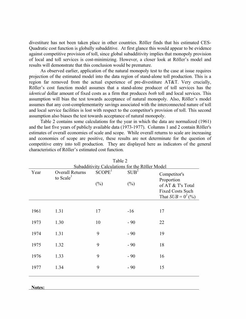
Table 2 contains some calculations for the year in which the data are normalized (1961) and the last five years of publicly available data (1973-1977). Columns 1 and 2 contain Röller's estimates of overall economies of scale and scope. While overall returns to scale are increasing and economies of scope are positive, these results are not determinate for the question of competitive entry into toll production. They are displayed here as indicators of the general characteristics of Röller’s estimated cost function.

Table 2

Subadditivity Calculations for the Röller Model Year Overall Returns

to Scale1 SCOPE1 (%)

SUB2 (%)

Competitor's Proportion of AT & T's Total Fixed Costs Such That SUB = 02 (%)

1961 1973 1974 1975 1976 1977

1.31 1.30 1.31 1.32 1.33 1.34

17 10 9 9 9 9

-16 - 90 - 90 - 90 - 90 - 90

17 22 19 18 16 15

Notes:

1. Taken from Röller (1990a). 2. Calculated by the present authors.

The calculations in column 3 contain more relevant information. SUB (see equation (26))

measures the degree of subadditivity in the Röller model associated with an industry structure in which pre-divestiture AT&T supplies all of the local service and 80 percent of the toll service demanded in the market, while a competitor supplies 20 percent of the toll service.26 The fact that SUB<0 indicates that, according to the Röller model, our chosen industry structure would have had higher costs than a monopoly structure. During the mid-seventies competition in the form specified here would have raised industry costs by approximately 9 percent.

The Röller model assumes that the fixed costs of all firms in the industry are identical. In the present context, this means that the competitor that supplies 20 percent of the toll market and is not involved in the supply of local services has the same dollar amount of fixed costs as AT&T, which supplies 80 percent of the toll market and 100 percent of local markets. Under such conditions it is not surprising that competition is estimated to be inefficient. In column 4 we calculate the effect of moderating Röller's assumption. The numbers in this column indicate the maximum fixed cost for the competitor, as a percentage of AT&T's total fixed cost, such that the competitive structure would be no more costly than the monopoly structure (i.e. SUB=0). The numbers in column 4 indicate that SUB=0 when the competitors fixed costs are 15 to 20 percent of AT&T's fixed costs. Any lower percentage results in the competitive structure being cost-minimizing.

How do we evaluate this result? The Röller model implies that as long as a competitor who supplied 20 percent of the U.S. toll market (and no local service) had fixed costs no higher than 15-20 percent of AT&T's total fixed costs, including fixed costs associated with the provision of local service, the presence of the competitor would not have increased industry costs. This fixed cost requirement does not seem to be very stringent, and hence we would conclude that the Röller model does not provide evidence against competitive entry. 4.2. Contemporary Evidence In the 1990s, economists have turned their attention to the Regional Bell Operating Companies (RBOC’s). The 1984 Divestiture Decree created seven RBOC’s, the holding companies that contained the 22 local operating companies of the former Bell System. Other non- Bell operating companies also existed and pre-dated 1984. These non-Bell companies ranged from larger groups such as GTE to city-specific carriers such as Cincinnati Bell27 and Rochester Tel. The data for these companies can prove fruitful for estimating local service returns to scale. However, many data problems exist. The source of data is the FCC’s Statistics of Communications Common Carriers. Moreover, these carriers provide local services, intra-

26 This division of the toll market was chosen to approximate the reality in the United States. Waverman

(1989, table 3) estimates that, as of 1986, AT&T supplied 82.3 percent of the U.S. inter-LATA (local access and transport area) interexchange market.

27 Cincinnati Bell was no longer a Bell company at the time of the divestiture, having repurchased its stock prior from AT&T prior to the divestiture.

LATA toll services, as well as access for long distance (inter-LATA) calling. Shin and Ying (1992, 1993) were the first to publish exploiting this data-base. They used

the pre-divestiture data for those RBOC’s, as well as data for non-Bell operating companies. They find modest scale economies at the sample mean,28 larger scale economies for the Bell companies,29 but no subadditivity of the cost function. They thus conclude that the break-up of the Bell System was justified on economic grounds and that competition at the local level can also be justified. Note that the work of Majumdar and Chang (1998) suggests this conclusion indirectly. Using DEA, they calculate the returns to scale characteristics of 38 operating companies belonging to RBOC’s as well as for non-Bell operating companies. They find that the majority of LEC’s do not enjoy scale efficiencies, and conclude that efficiencies can be gained by an industry restructuring whereby the RBOCs are downsized while the independent operators might be allowed to expand.30

Gabel and Kennet (1994) dispute the findings of Shin and Ying. They find positive economies of scope between switched and non-switched services, which decrease with customer density, and strong economies of scope, regardless of customer density, within the switched telephone market. Gabel and Kennet utilize an engineering optimisation model, rather than an econometric cost function. While the engineering approach permits much more attention to the details of network configuration than does the econometric approach, it does have some drawbacks. First, non-capital costs are either excluded or treated in an ad hoc manner. Typically, these costs constitute 40 to 50 percent of annual operating costs. Second, the optimisation requirement, which is central to the model, may not be reached in actual practice and there is no way to take this discrepancy into account. Third, the model assumes that the network can be configured as if there were no fixed assets currently in place. Adding assets to an existing network may have very different cost implications compared to starting from scratch.31

Krouse et al. (1999) is a recent analysis of telecommunications technology at the local level. Their data set includes all 22 local Bell Companies that were organized into the 7 RBOCs. The time period covered is 1978-1993 period. Four outputs are considered: residential access lines, business access lines, local calls and toll calls. However, in their estimation they find that the two measures of calling have no discernible impact on costs. Thus, the only outputs considered empirically are the numbers of residential and business lines. Krouse et al. report an overall cost elasticity of 1.127 at the sample mean, indicative of diseconomies of scale. They do not report estimates of economies of scope or tests of subadditivity, since the paper is concerned primarily with the impact of divestiture and deregulation on cost efficiency.

28 Their estimated overall cost elasticity at the sample mean is 0.958, which implies a scale elasticity of

1/0.958 = 1.04. 29 Described in Shin and Ying (1992). 30 Krouse et al. (1999) criticise Ying and Shin for not incorporating state specific regulation in their analysis.

Shin and Ying, however, do include state specific dummy variables in their analysis that mitigates this issue to some extent. The period of the data set (1976-83) used by Shin and Ying predates the significant changes in regulatory oversight associated with incentive regulation.

31 The scale economies inherent in the LECOM engineering cost model used by Gabel and Kennet can be seen by results presented in Gasmi, Laffont and Sharkey (1999) who utilize the same model. For the output range considered by Gasmi et al., the scale elasticity ranges from 2.78 to 6.25, which is considerably greater than that found in econometric studies that use historical data.

5. CONCLUSIONS Applied econometrics is just economic history seen through a model-oriented lens. The technical complexity of many of the econometric models of the telecommunications production technology should not obscure the fact that the empirical results can be no better than the relevance of the models' assumptions and the data used for estimation. On both counts, the econometric evidence that is reviewed in this does not seem to pass the relevancy test and be of use to economists in proposing structural changes to the telecommunications markets.

To be of relevance in these situations, the econometric models must be capable of estimating the production technology of a stand-alone toll producer. This is not the case. Nearly all of the potentially relevant models that have been estimated to date assume that the fixed costs of production are identical for a stand-alone toll producer and a producer of both toll and local services. This assumption biases the results towards a finding of natural monopoly service provision. The data sets used to estimate the models are drawn from an historical range of data far removed from the experience of a stand-alone toll producer. Extension of a cost function estimated from the available historical data to the toll-only producer's data range requires a leap of faith. That has no place in public policy proceedings.

The emerging competitive market structures will eventually provide the data necessary for the estimation of the cost functions required to test the natural monopoly hypothesis in telecommunications. The entrepreneurial experiments that competitors undertake will have an impact on the consequent evolution of industry structure in the various telecommunications segments. Such experiments will generate the information that can lead to evaluations of market structure, if such evaluations are still warranted. 32

There are also new developments in estimation methods, particularly of the non-parametric variety, that are potentially useful for the evaluation of production structures of firms. Applications of these techniques to new data may shed light on the issues under contention. Until that time, econometric evidence of the type surveyed in this paper should not, and has appeared not to, influence regulators’ decisions regarding permissible market structures.

REFERENCES Banker, R. D. 1990, Discussion: Comments on evaluating performance in regulated and

unregulated markets: A collection of fables, in J. R. Allison and D. L. Thomas, eds., Telecommunications Deregulation: Market Power and Cost Allocation issues, Westport, CT: Quorum Books.

Banker, R. D., H. Chang and S. K. Majumdar, 1996, Profitability, productivity and price recovery patterns in the U.S. telecommunications industry, Review of Industrial Organization, 11, 1-17.

Banker, R. D., A. Charnes and W. W. Cooper, 1984, Some models for estimating technical

32 By the time the required evidence becomes available, it is likely that competition will be so firmly

established (at least in the USA) so as to be irreversible.

and scale efficiencies in data envelopment analysis, Management Science, 30, 9, 1078-1092

Berndt, E. R. and M. A. Fuss, 1986, Productivity measurement with adjustments for variations in capacity utilization and other forms of temporary equilibrium, Journal of Econometrics, October/November, 7-29.

Berndt, E. R. and M. A. Fuss, 1989, Economic capacity utilization with multiple outputs and multiple inputs, NBER Working Paper No. 2932, Cambridge, MA, April.

Bernstein, J. I., 1988, Multiple outputs, adjustment costs and the structure of production, International Journal of Forecasting, 4, 207-219.

Bernstein, J. I., 1989, An examination of the equilibrium specification and structure of production for Canadian telecommunications, Journal of Applied Econometrics, 4, 265-282.

Breslaw, J. and J. B. Smith, 1980, Efficiency, equity and regulation: An econometric model of Bell Canada, Final Report to the Department of Communications, March.

Caves, D. W. and L. R. Christensen, 1980, The relative efficiency of public and private firms in a competitive environment: The case of Canadian railroads, Journal of Political Economy, 88, 958-976.

Charnes, A., W. W. Cooper and E. L. Rhodes, 1978, Measuring the efficiency of decision making units, European Journal of Operations Research, 2, 429-444.

Charnes, A., W. W. Cooper and T. Sueyoshi, 1988, A goal programming/constrained regression review of the Bell SystemBell Systems breakup, Management Science, 34, 1-26.

Christensen Associates, 1985, United States postal service real output, input and total factor productivity, 1963-1984, Report to Charles Guy, Director, Office of Economics, United States Postal Service, Washington, D.C.; October.

Christensen Associates, 1990, United States postal service annual total factor productivity, report to Charles Guy, Director, Office of Economics, United States Postal Service, Washington, D.C., March.

Crandall, R. W. and L. Waverman, 1995, Talk is cheap: The promise of regulatory reform in North American telecommunications, Washington, D. C.: The Brookings Institution.

Curien, N., 1991, The theory and measurement of cross-subsidies: An application to the telecommunications industry, International Journal of Industrial Organization, 9, 73-108.

Davis, O. A. and E. L. Rhodes, 1990, Evaluating performance in regulated and unregulated markets: A collection of fables, in J. R. Allison and D. L. Thomas, eds., Telecommunications deregulation: Market power and cost allocation issues, Westport, CT: Quorum Books.

Denison, E. N., 1985, Trends in American economic growth, 1929-1982, Washington, D. C.: The Brookings Institution.

Denny, M., M. Fuss and L. Waverman, 1981, The measurement and interpretation of total factor productivity in regulated industries, with an application to Canadian telecommunications in T. Cowing and R. Stevenson, eds., Productivity Measurement in Regulated Industries, New York: Academic Press.

Diewert, W. E. 1976, Exact and superlative index numbers, Journal of Econometrics, 4, 115-145.

Diewert, W. E. and T. J. Wales, 1991a, Multiproduct cost functions and subadditivity tests: A

critique of the Evans and Heckman research on the U.S. Bell System, Department of Economics, University of British Columbia Discussion Paper No. 91-21, June.

Diewert, W. E. and T. J. Wales, 1991b, On the subadditivity of telecommunications cost functions: Some empirical results for the U.S. and Japan, Department of Economics, University of British Columbia, Vancouver, Canada.

Elixmann, D., 1990, Econometric estimation of production structures: The case of the German telecommunications carrier, Diskussionsbeiträge Nr. 57, Wissenschaftliches Institut fur Kommunikationsdienste, Bad Honnef, Germany, April.

Evans, D. S. and J. J. Heckman, 1983, Multiproduct cost function estimates and natural monopoly tests for the Bell system, in D.S. Evans, ed., Breaking Up Bell: Essays on Industry Organization and Regulation, Amsterdam: North-Holland.

Evans, D. S. and J. J. Heckman, 1984, A test for subadditivity of the cost function with an application to the Bell SystemBell Systems, American Economic Review,74, 615-23.

Evans, D. S. and J. J. Heckman, 1986, Erratum: A test for subadditivity of the cost function with an application to the Bell system, American Economic Review, 76, 856-58.

Evans, D. S. and J. J. Heckman, 1988, Natural monopoly and the Bell System: Response to Charnes, Cooper and Sueyoshi, Management Science, 34, 27-38.

Fraquelli, G. and D. Vannoni, 2000, Multidimensional performance in telecommunications regulation and competition: Analysing the European major players, Information Economics and Policy, 12, 27-46

Fuss, M. A., 1983, A survey of recent results in the analysis of production conditions in telecommunications, in L. Courville, A. de Fontenay and R. Dobell, eds., Economic Analysis of Telecommunications: Theory and Applications, Amsterdam: North-Holland.

Fuss, M. A., 1992, Econometric evidence on scale, scope and the presence of natural monopoly: What can it tell us about the desirability of competition in public long-distance telephone service? University of Toronto Working Paper No. 9210.

Fuss, M. A., 1994, Productivity growth in Canadian telecommunications, Canadian Journal of Economics, 27, 2, 371-392.

Fuss, M. and L. Waverman, 1977, Multi-product, multi-input cost functions for a regulated utility: The case of telecommunications in Canada, paper presented at the NBER Conference on Public Regulation, Washington, D.C., December.

Fuss, M. and L. Waverman, 1981a, Regulation and the multi-product firm: The case of telecommunications in Canada, in Gary Fromm, ed., Studies in Public Regulation, Cambridge, MA: MIT Press.

Fuss, M. and L. Waverman, 1981b, The regulation of telecommunications in Canada, Technical Report No. 7, Ottawa: Economic Council of Canada.

Gable, D. and D. M. Kennet,:, 1994, Economies of scope in the local telephone exchange market, Journal of Reguatory Economics, 6, 381-98.

Gasmi, F., J-J. Lafont, and W. W. Sharkey, 1997, Incentive regulation and the cost structure of the local telephone exchange network. Journal of Regulatory Economics, 1997, 12, 5-25

Gentzoglanis, A. and R. D. Cairns, 1989, Cost comparisons and natural monopoly issues for two Canadian telecommunications carriers: Bell Canada and Alberta Government Telephones, paper prepared for presentation to the Bellcore-Bell Canada Conference on

Telecommunications Costing in a Dynamic Environment, San Diego. Guldmann, J-M., 1990, Economies of scale and density in local telephone networks, Regional

Science and Urban Economics, 20, 521-535 Jha, R. and S. K. Majumdar, 1999, A matter of connections: OECD telecommunications sector

productivity and the role of cellular technology diffusion, Information Economics and Policy, 11, 243-269

Jorgensen, D. W. and Z. Griliches, 1967, The explanation of productivity change, Review of Economic Studies, 34, 249-283

Kim, M. and J. Weiss, 1989, Total factor productivity growth in banking, Journal of Productivity Analysis, 139-153.

Kiss, F., 1983, Productivity gains in Bell Canada, in L. Courville, A. de Fontenay, and R. Dobell, eds., Economic Analysis of Telecommunications: Theory and Applications, Amsterdam: North-Holland.

Lippman, S. A. and R. P. Rumelt, 1982, Uncertain imitability: An analysis of interfirm differences in efficiency under competition, Bell Journal of Economics, 13, 413-438.

Maddala, G. S., 1977, Econometrics, New York: McGraw Hill. Majumdar, S. K., 1995, X-efficiency in emerging competitive markets: The case of U.S.

telecommunications. Journal of Economic Behavior and Organization, 26, 129-44. Majumdar, S. K. and H-H. Chang, 1998, Optimal local exchange carrier size, Review of

Industrial Organization, 13, 637-649 Ngo, H., 1990, Testing for natural monopoly: The case of Bell Canada, paper at the 1990

Meetings of the Canadian Economics Association, Victoria, B.C. Olley, R. E. and C. D. Le, 1984, Total factor productivity of Canadian telecommunications

carriers, Project Report to The Department of Communications and to Members of the Canadian Telecommunications Carriers Association, Ottawa, January.

Panzar, J., 1989, Technological determinants of firm and industry structure, in R. Schmalensee and R. D. Willig, eds., Handbook of Industrial Organization, Vol. I, Amsterdam: North-Holland.

Pulley, L. B. and Y. M. Braunstein, 1990, A new cost function for multiproduct technologies: Specification, estimation, and applications of the composite model, Mimeo, College of William and Mary, Williamsburg.

Röller, L-H., 1990a, Proper quadratic cost functions with an application to the Bell system, The Review of Economics and Statistics, 72, 202-210.

Röller, L-H , 1990b, Modelling cost structure: The Bell System revisited, Applied Economics, 22, 1661-1674.

Seiford, L. M., 1996, Data envelopment analysis: The evolution of the state of the art, 1978-1995, Journal of Productivity Analysis, 7, 99-137.

Seiford, L. M. and R. M. Thrall, 1996, Recent developments in DEA: The mathematical programming approach to frontier analysis, Journal of Econometrics, 46, 7-38.

Shin, R. T. and J. S. Ying, 1992, Unnatural monopolies in local telephone, RAND Journal of Economics, 23, 171-183

Simar, L. and P. Wilson, 2000, A general methodology for bootstrapping in non-parametric frontier models, Journal of Applied Statistics, 27, 779-802.

Solow, R. M., 1957, Technical change and the aggregate production function, Review of

Statistics and Economics, 39, 312-320. Uri, N. D., 2001, Technical efficiency, allocative efficiency, and the impact of incentive

regulation in telecommunications in the United States, Structural Change and Economic Dynamics, 12, 59-73

Waverman, L., 1989, U.S. interexchange competition in R.W. Crandall and R. Flamm, eds., Changing the rules: Technological Change, International Competition, and Regulation in Communications, Washington, D.C.: The Brookings Institution.

Wilson, P., 1993, Detecting outliers in deterministic nonparametric frontier models with multiple outputs, Journal of Business and Economic Statistics, 1993, 319-323.

Wilson, W. W. and Y. Zhou, 2001, Telecommunications deregulation and subadditive costs: Are local telephone monopolies unnatural? International Journal of Industrial Organization, 19, 909-930.

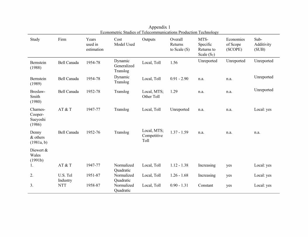
Appendix 1 Econometric Studies of Telecommunications Production Technology

Study Firm Yearsused in estimation

Cost Model Used

Outputs OverallReturns to Scale (S)

MTS- Specific Returns to Scale (ST)

Economies of Scope (SCOPE)

Sub- Additivity (SUB)

Bernstein (1988)

Bell Canada 1954-78 Dynamic Generalized Translog

Local, Toll 1.56 Unreported Unreported Unreported

Bernstein (1989)

Bell Canada 1954-78 Dynamic Translog

Local, Toll 0.91 - 2.90 n.a. n.a. Unreported

Breslaw-Smith (1980)

Bell Canada 1952-78 Translog Local, MTS; Other Toll

1.29 n.a. n.a. Unreported

Charnes- Cooper- Sueyoshi (1986)

AT & T 1947-77 Translog Local, Toll Unreported n.a. n.a. Local: yes

Denny & others (1981a, b)

Bell Canada 1952-76 Translog Local, MTS; Competitive Toll

1.37 - 1.59 n.a. n.a. n.a.

Diewert & Wales (1991b) 1. 2. 3.

AT & T U.S. Tel Industry NTT

1947-77 1951-87 1958-87

Normalized Quadratic Normalized Quadratic Normalized Quadratic

Local, Toll Local, Toll Local, Toll

1.12 - 1.38 1.26 - 1.68 0.90 - 1.31

Increasing Increasing Constant

yes yes yes

Local: yes Local: yes Local: yes

Appendix 1 (Continued) Econometric Studies of Telecommunications Production Technology

Study Firm Yearsused in estimation

Cost Model Used

Outputs OverallReturns to Scale (S)

MTS- Specific Returns to Scale (ST)

Economies of Scope (SCOPE)

Sub- additivity (SUB)

Elixmann (1990)

Deutsche Bundespost

1962-86 GeneralizedTranslog

Local, Toll 0.77 - 1.30 Unreported Unreported Unreported

Evans-Heckman (1983-84; 1986 revision, 1988)

AT & T 1947-77 Translog Local, Toll Un- reported

n.a.

n.a. Local: no

Fuss-Waverman (1977, 1981a)

Bell Canada 1952-75 Translog Local, MTS; Competitive Toll

0.89-1.15 n.a. n.a. Unreported

Fuss- Waverman (1981b) 1. 2.

Bell Canada Bell Canada

1957-77 1957-77

Translog Hybrid Translog

Local, MTS; Competitive Toll Local, MTS; Competitive Toll

1.26-1.63 0.83-1.09

n.a. Unreported

n.a. Unreported

Unreported Unreported

Gentzoglanis & Cairns (1989)

Bell Canada AGT

1952-86 1974-85

Translog Translog

Local, Toll Local, Toll

1.54 1.06

Unreported Unreported

Unreported Unreported

Local: yes Local: yes

33

Appendix 1 (Continued) Econometric Studies of Telecommunications Production Technology

Study Firm Yearsused in estimation

Cost Model Used

Outputs OverallReturns to Scale1 (S)

MTS- Specific Returns to Scale (ST)

Economies of Scope (SCOPE)

Sub- Additiity (SUB)

Kiss & Others (1981, 1983) Preferred 2 output

Bell Canada

1952-78

Generalized Translog

Local, Toll

1.62

1.09

0.09

Unreported

Ngo (1990) 1. 2. 3.

Bell Canada Bell Canada Bell Canada

1953-87 1953-87 1953-87

Generalized Translog Generalized Translog Generalized Translog

Local, Toll Local, Toll Local, Toll

1.01-2.42 0.75-2.05 0.83-1.72

Unreported " "

Unreported "

Local: yes Local: yes Local: yes

Pulley & Braunstein (1990)

AT & T 1947-77 Composite Local, Toll Unreported but S > 1

Unreported Unreported Expanded local: yes; not statistically significant

Röller (1990a) 1. 2.

AT & T AT & T

1947-79 1947-79

CES- Quadratic CES- Quadratic

Local, Toll Local, Intra, Inter

1.28-1.56 1.68-2.90

Unreported Unreported

0.07-0.34 0.61-0.95

Global: yes Global: yes

34

Appendix 1 (Continued) Econometric Studies of Telecommunications Production Technology (Studies on the Local Services Sector)

Study Firm Yearsused in estimation

Cost Model Used

Outputs OverallReturns to Scale1 (S)

Local Specific Returns to Scale (ST)

Economies Of Scope (SCOPE)

Sub- additivity (SUB)

Shin and Ying (1992, 1993)

58 LEC’s and RBOC’s

1976 – 1983 Translog Customer access, exchange, toll merge

0.958(local)

Notsubadditive

Gabel & Kennet (1993)

n.a.

1990 Engineeringcost model

Switched toll, exchange services, local private line services, toll private line service

n.a. n.a. Scope economies other than private line services. Diseconomies between private line and exchange services. Economies disappear in dense exchanges.

n.a.

Gasmi, Laffont & Sharkey (1997)

n.a. n.a. Translog onoutput of engineeriing model

CCS per customer; number of customers held constant

0.3 Unreported Expanded Local: yes but not significant statistically Krouse et al.

(1999) 22 RBOC’s 1978 - 1993 Translog Intra LATA

toll

Unreported